comparison of robotic total stations for scanning of ... of southern queensland . faculty of...
TRANSCRIPT
University of Southern Queensland
FACULTY OF ENGINEERING AND SURVEYING
Comparison of Robotic Total Stations
for Scanning of Volumes or Structures
A dissertation submitted by
Mr. Jeffrey Francis Jones
In fulfilment of the requirements of
Courses ENG4111 and ENG4112 Research Project
Towards the degree of
Bachelor of Spatial Science: Surveying
Submitted: 29 October 2009
ABSTRACT
Today’s society demand faster, easier, safer and more accurate spatial information
than ever before. Over the past 15 years surveyors have seen the introduction of
reflectorless technology and more recently, laser scanning. Reflectorless technology
and laser scanning has become a useful tool in many surveying applications. This
technology has opened the door to the majority of demands that the community and
other surveyors request. Due to this evolving technology specific laser scanning
instruments have been developed. These instruments can cost in excess of half a
million dollars and require specific software. In recent times companies have
introduced laser scanning capabilities into total stations to reduce costs and integrate
technology, which has launched the new evolution in total stations with most now
having reflectorless and scanning capabilities included within the instrument.
This project was undertaken to address surveyor’s uncertainties regarding
reflectorless technology and laser scanning capabilities within total stations. A
number of tests were conducted by both the Leica 1205R and the Trimble S6
instruments to compare both accuracy and performance. The three tests performed
varied from simple point comparisons to scanning of volumes and the measuring of
building encroachments. The results found there to be very small errors when
performing simple point comparisons over a small range. The total stations also
performed very well in the volume scans as both instruments produced similar results.
Lastly, some problems were found with the encroachment testing as software
capabilities limited my outputs. Both reflectorless and the laser scanning capabilities
performed very well allowing me to test and analyse their full potential.
i

ii
University of Southern Queensland
Faculty of Engineering and Surveying
ENG4111 Research Project Part 1 &
ENG4112 Research Project Part 2
LIMITATIONS OF USE
The council of the University of Southern Queensland, its Faculty of Engineering and
Surveying, and the staff of the University of Southern Queensland, do not accept any
responsibility for the truth, accuracy or completeness of the material contained within
or associated with this dissertation.
Persons using all or any part of this material do so at their own risk, and not at the risk
of the Council of the University of Southern Queensland, its Faculty of Engineering
and Surveying or the staff of the University of Southern Queensland.
This dissertation reports an educational exercise and has no purpose or validity
beyond this exercise. The sole purpose of the course pair entitled “Research Project”
is to contribute to the overall education within the student’s chosen degree program.
This document, the associated hardware, software, drawings, and other material set
out in the associated appendices should not be used for any other purpose: if they are
so used, it is entirely at the risk of the user.
Professor Frank Bullen
Dean
Faculty of Engineering and Surveying

CERTIFICATION
I certify that the ideas, designs and experimental work, results, analysis and
conclusions set out in this dissertation are entirely my own effort, except where
otherwise indicated and acknowledged.
I further certify that the work is original and has not been previously submitted for
assessment in any other course or institution, except where specifically stated.
Jeffrey Francis Jones
Student Number: 0050041009
_________________________
Signature
_________________________
Date
i

ACKNOWLEDGEMENTS
I would like to thank my supervisor, Mr. Kevin McDougall, from the University of
Southern Queensland Faculty of Engineering and Surveying, for his advice and
guidance. I would like to acknowledge his time and help given during the duration of
this project.
I would also like to acknowledge the University of Southern Queensland Faculty of
Engineering and Surveying for providing the equipment and Mr. Clinton Caudell for
all of his help with using the equipment during this project.
Finally I would like to thank family, friends and Krysten Cunningham for their help
and support during the year and the duration of my degree.
ii

TABLE OF CONTENTS
Content Page ABSTRACT .................................................................................................................... i
LIMITATIONS OF USE ............................................................................................... ii
CERTIFICATION .......................................................................................................... i
ACKNOWLEDGEMENTS ........................................................................................... ii
TABLE OF CONTENTS ............................................................................................. iii
LIST OF FIGURES ...................................................................................................... vi
LIST OF TABLES ....................................................................................................... vii
LIST OF APPENDICES ............................................................................................ viii
GLOSSARY OF TERMS ............................................................................................. ix
Chapter 1 – Introduction ............................................................................................ 1
1.1 Outline.................................................................................................... 1
1.2 Project Background ................................................................................ 1
1.3 Statement of Problem ............................................................................. 3
1.4 Project Aim ............................................................................................ 3
1.5 Objectives .............................................................................................. 3
1.6 Justification ............................................................................................ 4
1.7 Summary: Chapter 1 .............................................................................. 4
Chapter 2 – Literature Review ................................................................................... 5
2.1 Introduction ............................................................................................ 5
2.2 Principle of Electronic Distance Measurement ...................................... 5
2.2.1 Pulsed Time of Flight Measurement .................................................. 5
2.2.2 Phased Shift Measurement ................................................................. 6
2.3 Characteristics of Electromagnetic Radiation (EMR) ........................... 7
2.3.1 Electromagnetic Wave (EM) ............................................................. 7
2.3.2 Electromagnetic Radiation ................................................................. 8
2.3.3 EMR Interactions ............................................................................... 9
2.3.4 Reflectance ....................................................................................... 11
2.3.5 Surfaces & Material ......................................................................... 12
2.3.6 Colours ............................................................................................. 12
iii

2.3.7 Wet Surfaces .................................................................................... 12
2.3.8 Non-reflective Surfaces ................................................................... 13
2.4 Reflectorless Technology ..................................................................... 13
2.5 Laser Scanning ..................................................................................... 14
2.5.1 Object Recognition .......................................................................... 16
2.5.2 Accurate Feature Measurements ...................................................... 17
2.6 Reflectorless Issues & Industry Problems ........................................... 18
2.7 Summary: Chapter 2 ............................................................................ 19
Chapter 3 – Methodology ........................................................................................ 20
3.1 Introduction .......................................................................................... 20
3.2 Equipment ............................................................................................ 20
3.2.1 Trimble S6 DR300+ ............................................................................ 20
3.2.2 Magdrive ............................................................................................. 21
3.2.3 Leica TCRP 1205 + R1000 ................................................................. 22
3.2.4 Robotic Total Station Comparison...................................................... 23
3.3 Comparison .......................................................................................... 23
3.3.1 Reflectorless Distance Measurements ............................................. 23
3.4 Test Designs ......................................................................................... 24
3.5 Controlled Surface Scan ...................................................................... 25
3.5.1 Data Acquisition .............................................................................. 26
3.5.2 Field Procedures ............................................................................... 26
3.5.3 Office Procedures ............................................................................. 26
3.6 Volume Scanning ................................................................................. 27
3.6.1 Data Acquisition .............................................................................. 28
3.6.2 Field Procedures ............................................................................... 29
3.6.3 Office Procedures ............................................................................. 29
3.7 Building Encroachment ....................................................................... 30
3.7.1 Data Acquisition .............................................................................. 31
3.7.2 Field Procedures ............................................................................... 31
3.7.3 Office Procedures ............................................................................. 31
3.8 Summary: Chapter 3 ............................................................................ 32
Chapter 4 – Results and Analysis ............................................................................ 33
4.1 Introduction .......................................................................................... 33
4.2 Controlled Surface Scan ...................................................................... 33
iv
4.2.1 Results .............................................................................................. 34
4.2.2 Analysis............................................................................................ 34
4.3 Volumetric Scan................................................................................... 34
4.3.1 Results .............................................................................................. 34
4.3.2 Analysis............................................................................................ 39
4.4 Encroachment Testing ......................................................................... 42
4.4.1 Results .............................................................................................. 42
4.4.2 Analysis............................................................................................ 43
4.4 Summary: Chapter 4 ............................................................................ 45
Chapter 5 – Discussion ............................................................................................ 46
5.1 Introduction .......................................................................................... 46
5.2 Discussion ............................................................................................ 46
5.2.1 Controlled Surface Scan .................................................................. 46
5.2.2 Volumetric Scan............................................................................... 48
5.2.3 Encroachment Testing ..................................................................... 53
5.3 Summary: Chapter 5 ............................................................................ 55
Chapter 6 – Recommendations & Conclusion ......................................................... 57
6.1 Introduction .......................................................................................... 57
6.2 Recommendations ................................................................................ 57
6.2.1 Further Research .............................................................................. 59
6.3 Conclusion ........................................................................................... 60
References ................................................................................................................ 61
Appendices ............................................................................................................... 64
v
LIST OF FIGURES
Content Page
Figure 2.1: Phase Shift (θ) used to calculate distance travelled..................................... 7
Figure 2.2: Electromagnetic Wave ................................................................................ 8
Figure 2.3: Electromagnetic Spectrum, with frequency and wavelength properties. .... 8
Figure 2.4: Electromagnetic Spectrum. ......................................................................... 9
Figure 2.5: Specular Reflection. .................................................................................. 10
Figure 2.6: Diffuse Reflection. .................................................................................... 10
Figure 2.7: EMR Interactions ...................................................................................... 11
Figure 2.8: Typical Spectral Signatures ....................................................................... 13
Figure 2.9: Laser Scanning Unit .................................................................................. 16
Figure 2.10: DR Corner Measurement Effect .............................................................. 17
Figure 2.11: Eccentric Point Measurement. ................................................................. 18
Figure 3.1: Trimble S6 ................................................................................................. 21
Figure 3.2: Leica 1205R + R1000 ............................................................................... 22
Figure 3.3: Controlled Surface Scan Area. .................................................................. 25
Figure 3.4: Surface Scan Errors ................................................................................... 27
Figure 3.5: Normal’s to Plane, Surface Scan ............................................................... 27
Figure 3.6: Volumetric Test, Simulated Stockpile....................................................... 28
Figure 3.7: Volumetric Test, Building Encroachment. ................................................ 30
Figure 4.1: Controlled Surface Scan, Best Fit Plane of the data. ................................. 33
Figure 4.2: Volumetric Test, Raw data Trimble S6, Terramodel. ............................... 35
Figure 4.3: Volumetric Test, volume model Trimble S6 #1, Terramodel. .................. 36
Figure 4.4: Volumetric Test, volume model Trimble S6 #2, Terramodel. .................. 36
Figure 4.5: Volumetric Test, error percentage for each data set. ................................. 39
Figure 4.6: Encroachment Test, 2D representation of the encroachment test. ............ 43
Figure 4.7: Encroachment Test, raw data in Cyclone #1. ............................................ 43
Figure 4.8: Encroachment Test, raw data in Cyclone #2. ............................................ 44
Figure 4.9: Encroachment Test, 3D representation of the encroachment test. ............ 44
Figure 4.10: Encroachment Test, Chainage and Offset Report Terramodel. ............... 45
vi

LIST OF TABLES Content Page
Table 3.1: Comparison between instruments over a range of categories. ................... 23
Table 4.1: Comparison between instruments. .............................................................. 34
Table 4.2: Comparison between instruments, 100% of data. ...................................... 36
Table 4.3: Comparison between instruments, 75% of data. ........................................ 37
Table 4.4: Comparison between instruments, 50% of data. ........................................ 38
Table 4.5: Comparison between instruments, 25% of data. ........................................ 38
vii

LIST OF APPENDICES
Content Page
Appendix A – Project Specification ............................................................................ 64
Appendix B – Trimble S6 Datasheet ........................................................................... 65
Appendix C – Leica TPS1200+ Datasheet .................................................................. 67
Appendix D – S6 Dry Conditions. ............................................................................... 69
Appendix E – S6 Wet Conditions. ............................................................................... 72
Appendix F – Leica Dry Conditions. ........................................................................... 75
Appendix G – Leica Wet Conditions. .......................................................................... 78
Appendix H – Chainage and Offset Report, Terramodel ............................................ 81
Appendix I – Encroachment Plan ................................................................................ 84
viii
ix
GLOSSARY OF TERMS
3D - Three Dimensional: A description of the spatial environment in reference to its
three dimensions.
Total Station: An electronic optical measuring unit used within modern day
surveying.
EDM - Electronic Distance Measurement: A device that measures the distance
from an instrument to an object by the use of a prism.
Reflectorless Total Station: A device that measures a distance to an object without
the need of a prism to reflect.
Accuracy: The degree of closeness of a measurement to the true value.
Precision: The degree of repeatability of measurements under unchanged conditions
that show the same result (may not be accurate).
Point Cloud: An array of three dimensional points in space.

Chapter 1 – Introduction
Chapter 1 – Introduction
1.1 Outline
This chapter will provide an outline of the project background, research problem,
objectives and justification for this project. The dissertation will describe some of the
fundamental characteristics of reflectorless technology, laser scanning and the
specifications of the chosen robotic total stations. It will also cover in detail the
comparisons between the robotic total stations in regards to their scanning capabilities
of volumes and structures. This technology is relativity new to the present time so
there is a need to increase the awareness of it and perhaps to solve answers and create
new questions for further developments in this field.
1.2 Project Background
In society today there is a demand for faster, easier and safer technology and methods.
While fulfilling the role as spatial scientists there is a definite need to gather
information ‘faster’, understand the operation of a wide range of instruments and
methods to perform surveying applications ‘easier’ and to allow the collection of data
where other methods could not vantage ‘safer’. Technology within spatial science has
evolved rapidly over the past ten years by refining the above needs not only for
surveyors but general society as well. Changes are evident with the successful
introduction of technology into the spatial science industry. An example of this is the
Global Positioning System (GPS) which is now seen as a must have device for many
surveying applications. GPS introduced methods of measurement from satellites
without the need of traditional traversing. From the introduction of this new
technology questions were raised of its capabilities. These questions included the
following: What range of accuracies does it achieve? Is it affected by obstructions?
Will this technology be useful to anyone?
Comparison of Robotic Total Stations for Scanning of Volumes or Structures 1

Chapter 1 – Introduction
After research was carried out, the spatial science industry saw GPS as a standalone
application and the next revolution in surveying methods. We are now one step
further into the future with GPS integrated into total stations and the inclusions of
robotic and reflectorless technology which exist in standalone systems incorporating
all functions.
A relatively new development in technology is ground-based laser scanning also
known as terrestrial laser scanning. Laser scanning has evolved from reflectorless and
robotic technology. It is the next generation of automated surveying. Laser scanning
provides faster data capture, easier setup and use of equipment and allows collection
of data where other methods could not vantage. This means it is also safer for users.
By meeting the current needs of today’s society, spatial science industries can now
perform more tasks at a reduced cost and time.
Laser scanning is becoming increasingly popular for many applications including the
monitoring of features and objects. Scanners are used to monitor high wall
movements in mine sites as they do not require a surveyor on the high wall. The
scanner can record thousands of points automatically and the risk of injury to
operators and assistants is minimised. Consequently, the need is increasing to start
testing and comparing this new technology so it is guaranteed to meet professional
and performance standards not only for the surveyors utilising it but also for the
clients involved in the project.
As the name suggests reflectorless technology does not require the use of a reflector
or prism to record the distances. Measurements are made by the instrument emitting a
beam of light towards a feature where it is reflected back to the instrument and a
distance is then calculated. There are two types of measurement; pulsed time of flight
(TOF) and phase based. These will be explained in greater detail later. Reflectorless
technology does have some limitations that need to be researched and these will also
be explained in greater detail further into this project paper.
Robotic total stations allow the control over an instrument via remote control
generally from the reflector’s range pole. The operator can control the instrument by
Comparison of Robotic Total Stations for Scanning of Volumes or Structures 2

Chapter 1 – Introduction
the remote control connecting to the instrument wirelessly. This can remove the need
for an assistant field hand as the operator can complete the task by themselves.
1.3 Statement of Problem
Although reflectorless technology has been around for a number of years, there has
been limited testing and availability of this technology. Problems encountered with
reflectorless technology include its effect on different materials, colours and distances
as well as safety issues and the uses of the technology. Upon investigating these
problems I hope new techniques will arise for further research and testing for
continuing projects.
1.4 Project Aim
This project seeks to compare the laser scanning capabilities and reflectorless
limitation of two robotic total stations for various surveying applications.
1.5 Objectives
The key objectives of this project are:
i. To research the existing laser scanning technology, capabilities and
specifications of both the Trimble S6 and Leica 1205R.
ii. Identify a rigorous testing regime (speed, accuracy etc) and range of possible
testing applications including stock piles, buildings and vegetation.
iii. Test the scanning capabilities on various features including soil, structural
features (roof heights, floor heights and window frames) and point
comparisons under different conditions.
iv. Analyse the outcomes of the test according to a range of criteria.
v. Discuss the implications of the results with respect to surveying organizations
and potential opportunities.
vi. If time permits extend the range of scanning tests and situations.
Comparison of Robotic Total Stations for Scanning of Volumes or Structures 3
Chapter 1 – Introduction
Comparison of Robotic Total Stations for Scanning of Volumes or Structures 4
1.6 Justification
It is important to realise the full capabilities and limitations of laser scanning and
reflectorless technology. Many people within the surveying industry are not aware of
errors and the uses these instruments are capable of performing. This project will test
performance, accuracy, applications, comparisons and modelling. These are the
necessary tools for laser scanning and reflectorless applications. It is essential to
provide awareness and real application results to provide information to the user
which is the intention of this project.
1.7 Summary: Chapter 1
As the project aim states this project will seek to compare the laser scanning
capabilities and reflectorless limitation of two robotic total stations for various
surveying applications. This project will review all available literature on the
technology of both laser scanning robotic total stations and the theory behind how
they work. It is anticipated that by the end of this dissertation the results will provide
answers to the objectives listed above and solve the problem encountered.
Chapter 2 – Literature Review
Chapter 2 – Literature Review
2.1 Introduction
This chapter will outline the relevant literature associated with reflectorless total
station scanning. It will also examine the technology of how reflectorless and laser
scanning operates. There is limited research that has been conducted on laser scanning
with robotic total stations, however there has been a considerable amount of research
on laser scanning in general. This review will provide the theory behind this
technology, its history and current uses.
2.2 Principle of Electronic Distance Measurement
Accurate measurements are very important in today’s surveying and engineering
society where we see countless disputes between where boundaries are located and
buildings are set out and also the need for accurate measurement of volumes. The
need for very accurate measurement is important as a base for any surveying
applications. Besides the plumb bob and tape, there are two basic forms of
measurement used by a total station. These two measuring types are pulsed time of
flight (TOF) and phase shift. Both these methods are used to achieve the same result
which is to take accurate measurements. They both achieve the same goal however
they use two different methods to achieve this. Although both methods look to
achieve the same goal, they both have their advantages and disadvantages in different
applications. Some instruments now are offering the option of both methods which
gives the option back to the surveyor to decide. The surveyor is therefore not limited
or disadvantaged without the other.
2.2.1 Pulsed Time of Flight Measurement
Pulsed time of flight (TOF) measurement is an active mode of measuring where the
instrument emits its own source of energy. In comparison, a passive mode of
Comparison of Robotic Total Stations for Scanning of Volumes or Structures 5

Chapter 2 – Literature Review
measurement relies on an external source of energy e.g. the sun. TOF measurement
works by emitting a light pulse of energy towards an object or surface that is being
measured. This pulse is timed from when it leaves the light emitting device to when it
is reflected back from the object to the instrument. Because the time (t) of the pulse is
recorded to and from we have to half the time to get the distance to the object.
Equation 2.1 outlines the calculation method. Distance, ρ, is found by speed of light,
c, multiplied by time of fight, t, divided by two.
Ρ = (c * t) / 2 (Equation 2.1)
Pulsed TOF method uses wide cone like laser pulses which is useful for long range
measuring but not as effective for short range measuring. This can also have an effect
on the accuracy of the measurement. This type of measurement method is also
dependant on the accuracy of the speed of light. In general terms, the speed of light is
measured in a controlled vacuum, whereas real world situations are not in a controlled
environment. Speed of light when passed through different materials, weather and
surfaces will change the speed of the light. TOF method is also more tolerant to
interference of the beam. Due to further refining of this technology the difference in
accuracy has now become insignificant (Hoglund & Large 2005).
2.2.2 Phased Shift Measurement
Phased shift measurements are calculated in a similar way to an EDM in older total
stations. Instead of using a laser light pulse like TOF, they transmit a modulated
optical measuring beam also know as a sine wave type beam (see figure 2.1). This
beam is emitted from the EDM towards a surface where it is reflected back to the
EDM. This allows for the comparison between the original sine wave and the
reflected sine wave producing a horizontal shift between waves called a ‘phase shift’.
This phase shift can then determine the distance travelled from the length of one cycle
by the number of cycles shifted.
Comparison of Robotic Total Stations for Scanning of Volumes or Structures 6

Chapter 2 – Literature Review
Figure 2.1: Phase Shift (θ) used to calculate distance travelled.
Source: (Wikipedia n.d. a) Phase shift measurement is considered to have a greater accuracy compared to the
TOF method. This is because the beam has a narrow field of view and it is not
affected by as many variables. However, the phase shift method is known to have a
limited range and is affected by interference which therefore makes it less desirable to
users to perform these measurements (Hoglund & Large 2005).
Reflectorless measurement can be seen as a form of remote sensing application.
Remote sensing can be defined as the science, art and technology associated with the
acquisition and analysis of data about an object, area or phenomenon without direct
contact. This definition has similar characteristics to reflectorless measurement used
by laser scanning (Mather 2004).
2.3 Characteristics of Electromagnetic Radiation (EMR)
2.3.1 Electromagnetic Wave (EM)
An electromagnetic (EM) wave (see figure 2.2) has two properties, the first being an
electrical field which varies in magnitude perpendicular to the direction of travel. The
second component is a magnetic field which varies in magnitude at right angles to the
electrical field. Both fields travel at the speed of light.
Comparison of Robotic Total Stations for Scanning of Volumes or Structures 7

Chapter 2 – Literature Review
Figure 2.2: Electromagnetic Wave
Source: (National Research Council Canada 2006)
2.3.2 Electromagnetic Radiation
Electromagnetic radiation (EMR) is a form of energy that has the properties of a
wave. Electromagnetic radiation has two components namely wavelength and
frequency. Wavelength is the length of one cycle and the frequency is the number of
wave cycles that are repeated per time period. From figure 2.3 below it can be seen
that the wavelength is the shortest towards the Gamma Ray end of the spectrum
giving out a higher frequency. Whereas, at the opposite end of the spectrum towards
the radar and infrared regions the wavelengths are longer and have less frequency.
Figure 2.3: Electromagnetic Spectrum, with frequency and wavelength properties.
Source: (University of Minnesota n.d.)
Different wavelengths play a major role in how features are gathered and represented
when EMR is used for measurement. If you have ever seen a photograph of
vegetation studies you will often see that the photo will misrepresent the true colours
of vegetation. They will be either displayed in fluorescent green or red. This is
Comparison of Robotic Total Stations for Scanning of Volumes or Structures 8

Chapter 2 – Literature Review
because different features are detectable by different wavelengths. In this case
vegetation has high reflectance in the infrared red spectrum allowing us to control
what colours will be shown for that region. Figure 2.4 represents a spectrum which is
a region defined by the measurement nanometres or terahertz and this is called the
electromagnetic spectrum. Electromagnetic spectrum is a range of all possible
electromagnetic radiation frequencies.
Figure 2.4: Electromagnetic Spectrum.
Source: (South Carolina Department of Natural Resources 2009) The visible light region ranges from 380nm to 760nm. This region on the spectrum is
where the wavelength is the strongest and most sensitive to our eyes. Humans cannot
see any other part of the spectrum beside the visible light region.
2.3.3 EMR Interactions
Various effects like scattering, transmission, atmospherics and absorption can
influence the path or return signal of a wavelength. Scattering is the affect that a
surface has on a wavelength. There are two types of scattering these are specular and
diffuse. Figure 2.5 represents specular type reflectance which often occurs on smooth
surfaces. This happens when the signal is reflected back in a mirror like form. Figure
2.6 shows diffuse reflectance occurring on rough surfaces making the signal reflect in
different directions.
Comparison of Robotic Total Stations for Scanning of Volumes or Structures 9

Chapter 2 – Literature Review
Figure 2.5: Specular Reflection.
Source: (Wikipedia n.d. b)
Figure 2.6: Diffuse Reflection.
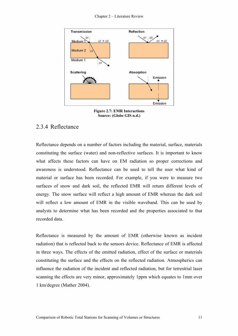
Source: (Wikipedia n.d. c) Figure 2.7 represents the four different effects of EMR interactions. Transmission
occurs when the EM radiation passes through the material/object without interaction,
like glass. The path can either be deflected or refracted as it passes through various
density materials. This can have an effect on the velocity and wavelength of the EM
radiation. Absorption occurs when the EM radiation is absorbed into the feature being
targeted. All surfaces and features absorb some amount of the EM radiation when it is
scanned. Some features though will absorb more EM radiation than others. The best
conductor of EM radiation is water. A good example of this conduction is when you
look down to the ocean from a plane in the air and you can see the dark blue tone in
the water. This is actually because the water absorbs all the EM radiation from the sun
giving the impression of dark blue water.
Comparison of Robotic Total Stations for Scanning of Volumes or Structures 10
Chapter 2 – Literature Review
Figure 2.7: EMR Interactions
Source: (Globe GIS n.d.)
2.3.4 Reflectance
Reflectance depends on a number of factors including the material, surface, materials
constituting the surface (water) and non-reflective surfaces. It is important to know
what affects these factors can have on EM radiation so proper corrections and
awareness is understood. Reflectance can be used to tell the user what kind of
material or surface has been recorded. For example, if you were to measure two
surfaces of snow and dark soil, the reflected EMR will return different levels of
energy. The snow surface will reflect a high amount of EMR whereas the dark soil
will reflect a low amount of EMR in the visible waveband. This can be used by
analysts to determine what has been recorded and the properties associated to that
recorded data.
Reflectance is measured by the amount of EMR (otherwise known as incident
radiation) that is reflected back to the sensors device. Reflectance of EMR is affected
in three ways. The effects of the emitted radiation, effect of the surface or materials
constituting the surface and the effects on the reflected radiation. Atmospherics can
influence the radiation of the incident and reflected radiation, but for terrestrial laser
scanning the effects are very minor, approximately 1ppm which equates to 1mm over
1 km/degree (Mather 2004).
Comparison of Robotic Total Stations for Scanning of Volumes or Structures 11

Chapter 2 – Literature Review
2.3.5 Surfaces & Material
Most surfaces and materials can be divided into the two common forms of scattering
being specular and diffuse. Specular surfaces and material will usually occur where
the EMR is reflected from relativity smooth objects like metal, walls, concrete and
any polished surfaces or coverings. Whereas, diffuse scattering will occur as EMR
reflects from rough surfaces and materials like asphalt, rendered bricks, rocks & dirt
and jagged features.
2.3.6 Colours
Coloured surfaces also absorb and reflect EMR. Colour is used in many ways to
define features and give objects identification. Reflectance is affected by moisture,
natural characteristics and different properties of the feature. For example, chlorophyll
which is a chemical of leaves will absorb the blue and red energy thus reflecting the
green wavelength. If the plant is stressed or matured, it will contain less chlorophyll,
resulting in less absorption and more reflection in the red energy waveband. Like all
other factors colour must be taken into account when analysing EMR (Mather 2004).
2.3.7 Wet Surfaces
One material that is an excellent conductor of EMR is clear water. Figure 2.8 shows
how water absorbs all EMR in the infrared (IR) band and only reflects a small amount
of EMR in the visible band. This is due to water being transparent and the absorption
of EMR. As the EMR reaches the water it absorbs it and transmission scattering
causes the radiation to scatter in all directions converting it into other forms of energy.
As mentioned above, clear water is an excellent conductor of EMR. However,
sometimes there is no need to measure clear water and instead just the things that are
suspended within it. Turbid water contains materials that are suspended within it
including dirt, sediments and algae. These suspended materials cause EMR to reflect.
Although it causes EMR to reflect the reflection is dependent on how turbid the water
is and what materials are being reflected. As surveyors the need to measure water is
not a common target except for surfaces that may contain water particles like dew or
Comparison of Robotic Total Stations for Scanning of Volumes or Structures 12

Chapter 2 – Literature Review
light rain. These water particles may cause small amounts of refraction from one
medium to the next altering the path of the radiation.
Figure 2.8: Typical Spectral Signatures
Source: (Google n.d.)
2.3.8 Non-reflective Surfaces
Not all EMR will reflect from every surface. Non-reflective surfaces include plain
glass, light coverings, windows, mirrors and water. The effects these surfaces have on
EMR are transmission scattering, where the radiation passes through the surface and
reflects from the next object it comes into contact with. As explained above, water has
very little reflection or sometimes none in the visible band. Plain clear glass will not
reflect any amount of radiation, but will refract the light radiation as it passes through
the glass. This refraction can cause the light beam to refract so far that it will not
reflect back to the instrument. In most cases this will be the reason why radiation is
not recorded by a laser scanning instrument.
2.4 Reflectorless Technology
Technology is continually evolving within the surveying industry with many new
instruments and methods being developed all the time. The method of measurement
used within surveying began with the use of the Gunter’s chain until surveyors saw
the introduction of the flat steel tape. Technology continued to progress with the use
of electronic distance measurement (EDM). EDM emits a light wave beam from a
device which then reflects from a prism target back to the EDM device. It then
Comparison of Robotic Total Stations for Scanning of Volumes or Structures 13

Chapter 2 – Literature Review
proceeds to calculate the distance acquired by the reflection. Nowadays, due to 21st
century technology the limitation of the prism has been removed with the introduction
of direct reflex (DR). This is also known as reflectorless which now sees
measurement taken directly to features without the use of other tools (Department of
Environment and Resource Management 2007).
Reflectorless technology has become essential to many surveyors in the industry. It is
able to provide numerous beneficial factors including the following:
• The ability to record information of features that might not have been accessible before due to safety issues.
• Automated systems and sole operators. • Time & costs.
While reflectorless technology is relatively new to surveying, the technology has been
around for quite some time. The latest trend of reflectorless technology has seen
almost all instruments now incorporate reflectorless technology as a standard into
surveying instruments. Reflectorless technology is opening a new door in one-person
surveying. By having reflectorless capabilities, GPS and robotics all integrated into
the one system there is no need for a traditional chainman. This increases the speed of
the work performed and also to some degree it improves accuracy and time efficiency.
2.5 Laser Scanning
Laser scanning can be defined as the scanning of a surface by the means of EM pulses
of energy that are measured by a laser scanning instrument. This then creates three-
dimensional (3D) points of data. Data is achieved by remotely sensing horizontal &
vertical angles and reflected distances. The data is in the form of X,Y,Z coordinates
which are based from the set parameters within the instrument. This data can then be
used to represent the real world in the form of coordinates for the analysis of
information and design on a computer display. Unlike most traditional surveying
instruments and methods, laser scanning can be performed any time of day or night
and also in varying weather conditions like rain or fog.
Comparison of Robotic Total Stations for Scanning of Volumes or Structures 14
Chapter 2 – Literature Review
There are two main forms of platforms that laser scanners use which are terrestrial
and airborne laser scanners. Airborne laser scanning uses a plane or helicopter as a
platform and performs scanning from the sky. Terrestrial laser scanning uses
platforms on the earth’s surface otherwise known as ground based. These platforms
come in the form of total station scanners and laser scanner units. They are used to
perform everything that an airborne laser scanner does but for ground features. Some
uses of terrestrial laser scanning are:
• Scanning cultural heritage features. • Archaeology studies and documenting. • Modelling building and structures. • Volumetric calculations of open and underground mining. • Forensic crime scene investigation. • Deformation monitoring of surfaces and structures. • Engineering and constructed surveys. • Monitoring of forestry, glaciers, landslides and dam walls. • Virtual reality computer games and animated walkthroughs. • Vegetation studies of growing rates and density studies.
These are just some of the uses of laser scanning. As research in this field expands,
new problems will arise and greater software will become available hopefully at
cheaper prices. A laser scanner will very soon become an everyday tool in the
collection of remote data.
The scanning ability in total stations today is becoming more and more automated.
This means that the operator sets it, defines some required parameters and lets it scan.
When comparing laser scanning to traditional surveying methods, there is not a great
deal of difference between the theoretical foundations. They both achieve X, Y, Z
point data, they both need computer analysis and they both produce the same project
result. However a laser scanner requires only one field technician, can scan up to
50,000 points a second, has an automated data system and takes measurements to
locations not accessible (See figure 2.9).
Comparison of Robotic Total Stations for Scanning of Volumes or Structures 15

Chapter 2 – Literature Review
Figure 2.9: Laser Scanning Unit
Source: (Google 2009)
2.5.1 Object Recognition
Analysis of gathered data can be quite difficult in some situations. Point data is
displayed as points on a computer screen in relation to the coordinates recorded. So
how do we know what each point represents? Without any prior knowledge of the
scanned area this would prove to be difficult. After some lengthy human analysis it
can be determined that points along common features like the edge of a building for
example can be defined. Features like window frames and roof guttering can start to
be distinguishable. This type of recognition can take quite some time and become
really frustrating. New software technology has recently evolved enabling computer
software to recognise point features along common lines and distances.
The software analyses and interrogates the data to find the trends and occurrences of
point data. For example, if a wall was to be scanned and it had a photo frame hanging
on it, the software could be used to define this feature. The software is capable of
recognising the straight line edges of the photo frame. This in conjunction with the
comparison of the vertical plane of the wall to the points on the frame can determine
that the points are raised away from the plane of the wall. If the software recognises
the wrong features this can still be undone and the drafter can manually adjust the
data. This software is not available with all drafting programs and is currently still in
development stages.
Comparison of Robotic Total Stations for Scanning of Volumes or Structures 16
Chapter 2 – Literature Review
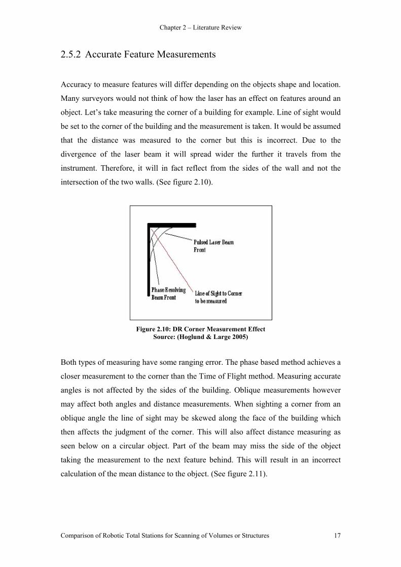
2.5.2 Accurate Feature Measurements
Accuracy to measure features will differ depending on the objects shape and location.
Many surveyors would not think of how the laser has an effect on features around an
object. Let’s take measuring the corner of a building for example. Line of sight would
be set to the corner of the building and the measurement is taken. It would be assumed
that the distance was measured to the corner but this is incorrect. Due to the
divergence of the laser beam it will spread wider the further it travels from the
instrument. Therefore, it will in fact reflect from the sides of the wall and not the
intersection of the two walls. (See figure 2.10).
Figure 2.10: DR Corner Measurement Effect
Source: (Hoglund & Large 2005)
Both types of measuring have some ranging error. The phase based method achieves a
closer measurement to the corner than the Time of Flight method. Measuring accurate
angles is not affected by the sides of the building. Oblique measurements however
may affect both angles and distance measurements. When sighting a corner from an
oblique angle the line of sight may be skewed along the face of the building which
then affects the judgment of the corner. This will also affect distance measuring as
seen below on a circular object. Part of the beam may miss the side of the object
taking the measurement to the next feature behind. This will result in an incorrect
calculation of the mean distance to the object. (See figure 2.11).
Comparison of Robotic Total Stations for Scanning of Volumes or Structures 17

Chapter 2 – Literature Review
Figure 2.11: Eccentric Point Measurement.
Source: (Hoglund & Large 2005)
2.6 Reflectorless Issues & Industry Problems
Surveying industries are faced with many problems every day, whether it is
instrument problems, project task problems or limitations due to Workplace Health &
Safety (WH&S). Hence there is the need for researchers and problem solving
personnel to create new methods or equipment to assist with these troublesome
applications. Three applications have been identified from general day to day
surveying tasks.
1. Volume scans: This involves the scanning to features that are restricted by
WH&S. They may be restricted due to surveyors in high places, physically
unable to reach the area or limited by equipment eg, cost of a laser scanning
instruments. The scanning of volumes in mines is very important and requires
a high level of accuracy. Because the materials they gather are exchanged for
money. Consequently, there is a need to understand the limitations and
accuracies of reflectorless scanning.
2. Building encroachments: This is where a building or feature has extended
beyond its property boundaries to encroach onto a neighbouring allotment or
crown land. For example ‘The Gabba’ in Brisbane sees part of the building
encroached onto the street reserve being crown land. As surveyors we have to
notify both the crown and the land owner and show the encroachment on a
plan. Due to the complexity of the encroachment, traditional surveying
Comparison of Robotic Total Stations for Scanning of Volumes or Structures 18
Chapter 2 – Literature Review
Comparison of Robotic Total Stations for Scanning of Volumes or Structures 19
methods would be expensive and difficult to exercise. This would see the use
of reflectorless technology to scan the area of the building encroachment in
relation to the boundaries.
3. Inaccessible areas: From the above two applications inaccessibility is a major
factor in some surveying tasks. Measuring points of a high rise building or
even clearances of power lines from trees are virtually inaccessible by
traditional survey methods due to high costs.
Reflectorless technology and scanning may be the best options for the above tasks,
but there are still some imperfections with this technology. Some issues include the
scanner captures too much data resulting in a long processing time. The ability to
analyse the data in real time and get results straight from the instrument. Also not all
materials reflect EMR and if a point does not reflect then the instrument keeps trying
to scan the point. From these three application problems I have chosen to conduct
small test designs to highlight the potential problems and methods for overcoming
them.
2.7 Summary: Chapter 2
In summary, this literature review has explored the technology used in the
undertaking of this project. This chapter has explored the background technology of
reflectorless measuring, laser scanning capability and the interaction EMR has with
various surfaces and materials. Research into this technology has warranted tests of
how the technology can be used effectively and the capabilities it may offer. The
information in this review has underlined the proceeding chapters and was used to
create the tests designs within the methodology.
Chapter 3 – Methodology
Chapter 3 – Methodology
3.1 Introduction
At present the principles, limitations and standards of robotic total station laser
scanning are limited to the general surveyor. Consequently, the opportunity has arisen
to research the capabilities, limitations and test this new technology over different
scenarios and problems. The aim of this chapter is to provide an understanding of how
this technology works over a number of features and also outline the field and office
techniques that underpin it. Explanation of the test sites that were used and how the
instruments went about the process are also discussed. The desired outcome of this
methodology is to compare both the Leica TCRP 1205 + R1000 & Trimble S6 on the
same test designs and provide users with performance feedback on the technology.
3.2 Equipment
3.2.1 Trimble S6 DR300+
The Trimble S6 is one of two total stations used for data acquisition within this
project. The S6 is a fully robotic instrument which caters for traditional survey
applications and more. The capabilities of the S6 include reflectorless technology,
onboard data storage, motorised robotic controlling and many other features. The S6
comes with a detachable controller screen interface for connection to computers,
robotic rover and GPS units. The Trimble CU controller comes with up-to-date
software for easy use between applications. The feature of the Trimble S6 that this
project is mainly concerned with is the application called “surface scan”. Surface scan
allows you to define the area that is to be scanned and the instrument will robotically
scan the area with rapid point capture. It will also store all the data in the onboard
memory card for easy downloading and analysis. This data can be viewed in notepad,
Microsoft XL, Terramodel and other drafting software. Angle and distance
measurement accuracy ranges from 2” – 5” angle measurement and 3mm with prism
Comparison of Robotic Total Stations for Scanning of Volumes or Structures 20
Chapter 3 – Methodology
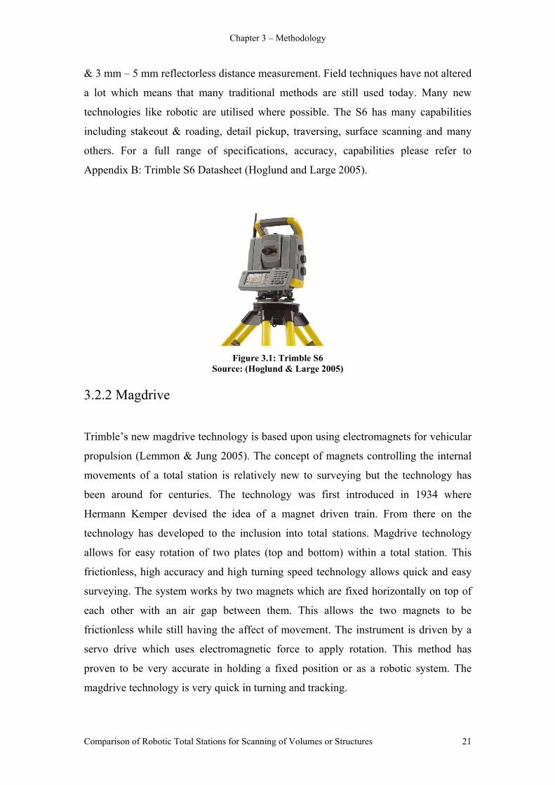
& 3 mm – 5 mm reflectorless distance measurement. Field techniques have not altered
a lot which means that many traditional methods are still used today. Many new
technologies like robotic are utilised where possible. The S6 has many capabilities
including stakeout & roading, detail pickup, traversing, surface scanning and many
others. For a full range of specifications, accuracy, capabilities please refer to
Appendix B: Trimble S6 Datasheet (Hoglund and Large 2005).
Figure 3.1: Trimble S6
Source: (Hoglund & Large 2005)
3.2.2 Magdrive
Trimble’s new magdrive technology is based upon using electromagnets for vehicular
propulsion (Lemmon & Jung 2005). The concept of magnets controlling the internal
movements of a total station is relatively new to surveying but the technology has
been around for centuries. The technology was first introduced in 1934 where
Hermann Kemper devised the idea of a magnet driven train. From there on the
technology has developed to the inclusion into total stations. Magdrive technology
allows for easy rotation of two plates (top and bottom) within a total station. This
frictionless, high accuracy and high turning speed technology allows quick and easy
surveying. The system works by two magnets which are fixed horizontally on top of
each other with an air gap between them. This allows the two magnets to be
frictionless while still having the affect of movement. The instrument is driven by a
servo drive which uses electromagnetic force to apply rotation. This method has
proven to be very accurate in holding a fixed position or as a robotic system. The
magdrive technology is very quick in turning and tracking.
Comparison of Robotic Total Stations for Scanning of Volumes or Structures 21

Chapter 3 – Methodology
3.2.3 Leica TCRP 1205 + R1000
The Leica TCRP 1205 + R1000 is the second instrument used for comparison within
this project. The Leica instrument is also fully robotic which includes all the
necessary features to carry out all surveying applications. Similar to the S6, Leica has
reflectorless technology, onboard data storage, motorised robotic controlling and
many other features. The Leica display unit comes with a dual colour screen display
for easy use and appearance. The instrument can also be used in conjunction with a
robotic smart pole unit for on-the-fly measurements and an integrated GPS unit. All
data is viewable on various software applications and Leica also provide an easy
single package called Leica Geo Office. The scanning program used is called
“Reference Line”. It works by defining a reference scan line which then allows you to
define the scanning parameters. Once these parameters have been defined the
instrument can perform the scan of the area. The instrument’s software allows
measurement spacing intervals to be set and a real time colour display of points
recorded. All data is stored in the onboard memory card which can be connected to
the computer for data transfer. Angle and distance measurement accuracy ranges from
5” angle measurement and 1 mm – 3 mm with prism & 2 mm – 4 mm reflectorless
distance measurement. Field techniques are similar to the S6 with the only differences
in software and procedures. The Leica has many capabilities including stakeout and
roading, detail pickup, traversing, reference lines and many others. For a full range of
specifications, accuracy and capabilities please refer to Appendix C: Leica TPS1200+
Datasheet (Hoglund & Large 2005).
Figure 3.2: Leica 1205R + R1000 Source: (Leica Geosystems 2009)
Comparison of Robotic Total Stations for Scanning of Volumes or Structures 22
Chapter 3 – Methodology
3.2.4 Robotic Total Station Comparison
In comparison both instruments have very similar features, capabilities and
applications. They are so similar that the main differences between them are the
colour, shape, brand, onboard software and display. Both instruments achieve the
same accuracy for angle and distance measurement. The Trimble S6 has been
designed to be more user friendly with easy setup and measuring. Compared to the
Leica 1205R this instrument is a little hard to control but that is based on the
individual user.
3.3 Comparison
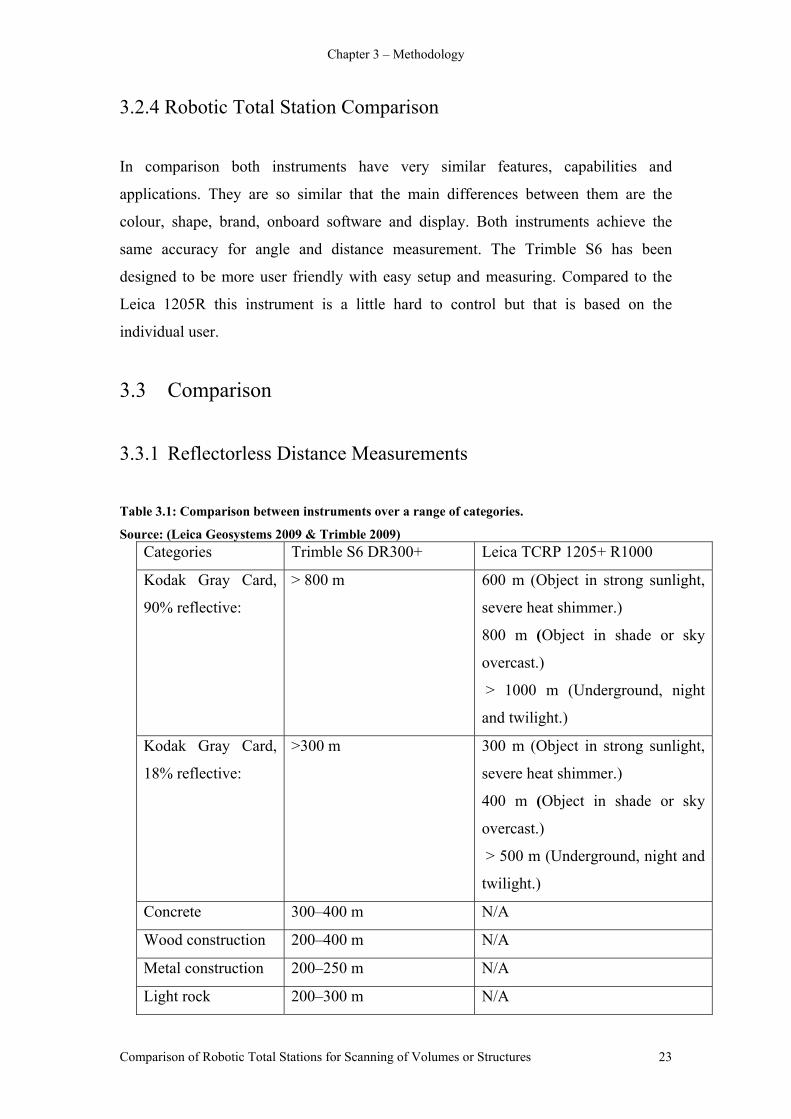
3.3.1 Reflectorless Distance Measurements Table 3.1: Comparison between instruments over a range of categories.
Source: (Leica Geosystems 2009 & Trimble 2009) Categories Trimble S6 DR300+ Leica TCRP 1205+ R1000
Kodak Gray Card,
90% reflective:
> 800 m 600 m (Object in strong sunlight,
severe heat shimmer.)
800 m (Object in shade or sky
overcast.)
> 1000 m (Underground, night
and twilight.)
Kodak Gray Card,
18% reflective:
>300 m 300 m (Object in strong sunlight,
severe heat shimmer.)
400 m (Object in shade or sky
overcast.)
> 500 m (Underground, night and
twilight.)
Concrete 300–400 m N/A
Wood construction 200–400 m N/A
Metal construction 200–250 m N/A
Light rock 200–300 m N/A
Comparison of Robotic Total Stations for Scanning of Volumes or Structures 23

Chapter 3 – Methodology
Dark rock 150–200 m N/A
Reflective foil 20
mm
800 m N/A
Reflective foil 60
mm
1600 m N/A
Shortest possible
range
2 m 1.5 m
Longest possible
range
1600 m 1200 m
Laser Beam Pulsed laserdiode 870nm,
laser class 1, Laser pointer
coaxial (standard) laser
class 2
Coaxial, visible red laser, Carrier
wave: 660 nm. Measuring system
Pinpoint R400/R1000: basis 100
MHz – 150 MHz
Angle accuracy 5” (1.5 mgon) 5” (1.5 mgon)
Distance accuracy 3 mm + 2 ppm or 5 mm +
2 ppm, standard
2 mm + 2 ppm (reflectorless < 500
m), 4 mm + 2 ppm (reflectorless >
500m), standard
Atmospherics
corrections
N/A N/A
Measuring time 1 – 5s / measurement 12s max (Reflectorless)
Motorized motor
speed
115° / s 45° / s
Weight 5.15kg (instrument) 4.8 – 5.5 kg
3.4 Test Designs
In this chapter I will outline the three test designs completed for the fulfillment of this
project. Test design one comprised of a relatively simply designed test to assess the
basic principles, concept and analysis of the instrument for time, accuracy and
processing. Test design two comprised of scanning a simulated stockpile for the
analysis and representation of the data. Test design three consisted of a more in depth
scan of surveying related applications like building encroachments and how
reflectorless technology can be used to measure and represent encroachments. This
Comparison of Robotic Total Stations for Scanning of Volumes or Structures 24

Chapter 3 – Methodology
chapter will cover all relative information about these designs and also the field and
office procedures that were used to perform them.
3.5 Controlled Surface Scan
Test design one was a basic replication of a field survey scan of a chosen feature. I
have chosen to perform a simple test to gain an understanding of the instruments and
portray simple results and conclusions to my readers. This test was performed under
controlled conditions, with both instruments scanning over a dry wall surface and then
a water spray surface. This allowed for easy analysis between the instruments for
accuracy, time and conditions. It also allowed me to evaluate the user friendliness of
both instruments.
Test one was carried out within the University of Southern Queensland (USQ)
grounds in room Z125. The testing surface was marked for permanency in case of
data failure or further and future testing. The test site was monitored under a room
temperature of 20 degrees Celsius and controlled conditions. Attention was made to
the testing wall as not all walls are exactly flat or when pointing the instrument to the
same location (see figure 3.3). This will cause small insignificant errors (less than
2mm difference).
Scan
Area
Figure 3.3: Controlled Surface Scan Area.
Comparison of Robotic Total Stations for Scanning of Volumes or Structures 25
Chapter 3 – Methodology
3.5.1 Data Acquisition
The area scanned for test design one is approximately a 0.500m by 0.500m squared
surface. This surface was scanned with both instruments at 0.050mm intervals both
horizontally and vertically. For this exercise there was an arbitrary coordinate system
set with an arbitrary back sight (BS) set for the purpose of testing.
3.5.2 Field Procedures
Testing procedures will be the same for both instruments where the instruments will
be similar except for the instruments software and display.
• After gathering all available equipment, one instrument is setup on the pillar
and an arbitrary BS set and coordinates given.
• After setup is completed, continue into the scanning software found for the
Leica instrument (Reference line) and the Trimble S6 (Surface scan).
• The scanning software will ask for the type of scan, parameters to be set and
the spacing interval. After all parameters have been entered, the scan will
initiate.
• The display screen will show how many points have been recorded and how
many have not. It also displays an estimated time for the completion of the
scan.
• Once the scan is completed all of the data is then stored within the total station
on a memory card for extraction to a computer.
• Follow these steps for both instruments and repeat the scan on both a dry wall
and a water spray surface. These steps may vary a little depending on the
instrument used as there will be slight differences in display modes and the
naming of applications.
3.5.3 Office Procedures
Once testing was completed, the data was extracted from both instruments into a
computer. The data was then imported into Terramodel where a report was conducted
Comparison of Robotic Total Stations for Scanning of Volumes or Structures 26
Chapter 3 – Methodology
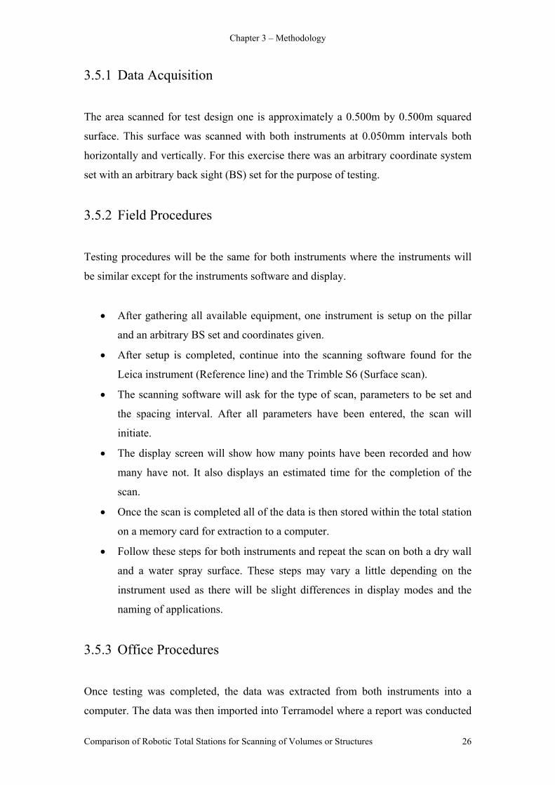
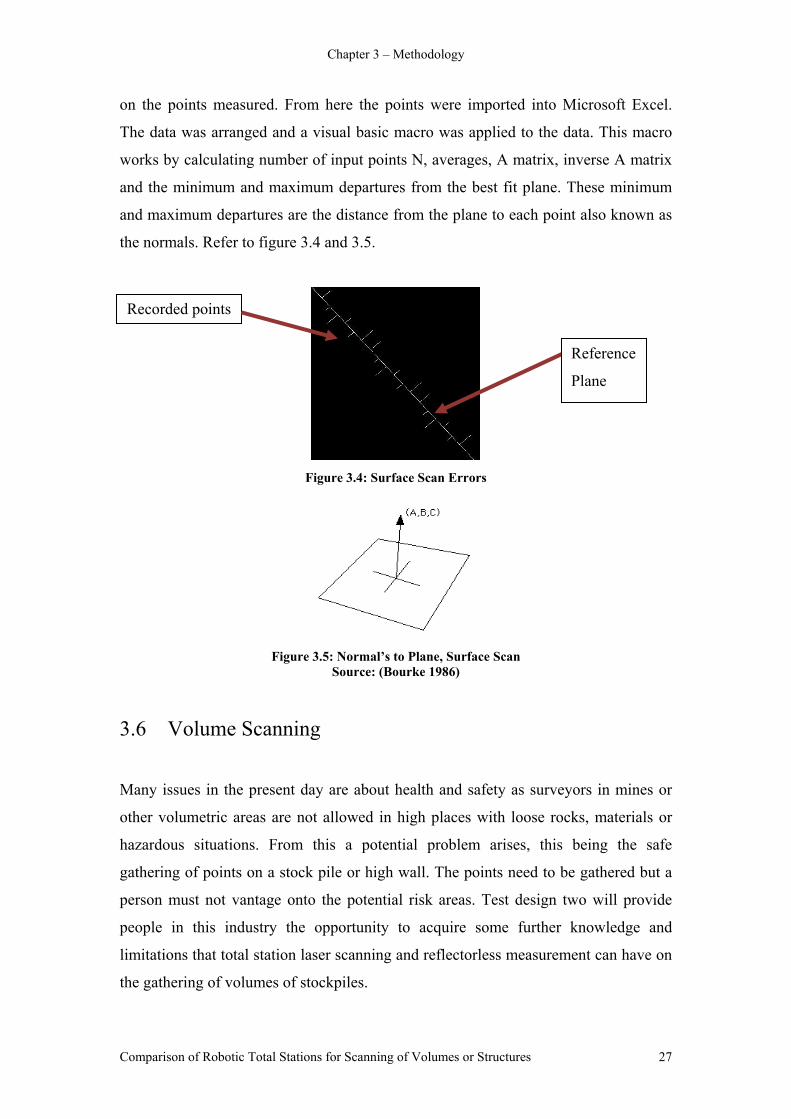
on the points measured. From here the points were imported into Microsoft Excel.
The data was arranged and a visual basic macro was applied to the data. This macro
works by calculating number of input points N, averages, A matrix, inverse A matrix
and the minimum and maximum departures from the best fit plane. These minimum
and maximum departures are the distance from the plane to each point also known as
the normals. Refer to figure 3.4 and 3.5.
Recorded points
Reference
Plane
Figure 3.4: Surface Scan Errors
Figure 3.5: Normal’s to Plane, Surface Scan
Source: (Bourke 1986)
3.6 Volume Scanning
Many issues in the present day are about health and safety as surveyors in mines or
other volumetric areas are not allowed in high places with loose rocks, materials or
hazardous situations. From this a potential problem arises, this being the safe
gathering of points on a stock pile or high wall. The points need to be gathered but a
person must not vantage onto the potential risk areas. Test design two will provide
people in this industry the opportunity to acquire some further knowledge and
limitations that total station laser scanning and reflectorless measurement can have on
the gathering of volumes of stockpiles.
Comparison of Robotic Total Stations for Scanning of Volumes or Structures 27

Chapter 3 – Methodology
Test site two is situated near the front entrance of the University of Southern
Queensland grounds. The scan was performed over a section of raised land used as a
retaining wall for water runoff. This section of land is covered by grass and is half
situated under tree cover. The site was marked out so repeatability of both instruments
could be achieved (See Figure 3.6).
Figure 3.6: Volumetric Test, Simulated Stockpile.
3.6.1 Data Acquisition
Due to software difficulties scanning was not able to be performed with the Leica
1205R. Instead reflectorless measurements were taken along the mound at my
discretion over the simulated stockpile for comparisons. The area scanned for test
design two is approximately one and a half metres high from natural surface, ten
metres wide and ten metres long. This surface was scanned with the Trimble S6 at
0.400mm interval both horizontally and vertically. For this exercise there was an
arbitrary coordinate system set with an arbitrary back sight (BS) set for the purpose of
testing.
Comparison of Robotic Total Stations for Scanning of Volumes or Structures 28
Chapter 3 – Methodology
3.6.2 Field Procedures
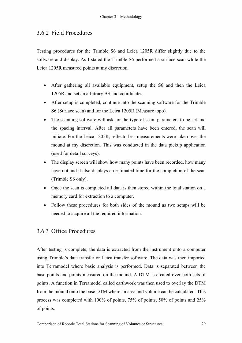
Testing procedures for the Trimble S6 and Leica 1205R differ slightly due to the
software and display. As I stated the Trimble S6 performed a surface scan while the
Leica 1205R measured points at my discretion.
• After gathering all available equipment, setup the S6 and then the Leica
1205R and set an arbitrary BS and coordinates.
• After setup is completed, continue into the scanning software for the Trimble
S6 (Surface scan) and for the Leica 1205R (Measure topo).
• The scanning software will ask for the type of scan, parameters to be set and
the spacing interval. After all parameters have been entered, the scan will
initiate. For the Leica 1205R, reflectorless measurements were taken over the
mound at my discretion. This was conducted in the data pickup application
(used for detail surveys).
• The display screen will show how many points have been recorded, how many
have not and it also displays an estimated time for the completion of the scan
(Trimble S6 only).
• Once the scan is completed all data is then stored within the total station on a
memory card for extraction to a computer.
• Follow these procedures for both sides of the mound as two setups will be
needed to acquire all the required information.
3.6.3 Office Procedures
After testing is complete, the data is extracted from the instrument onto a computer
using Trimble’s data transfer or Leica transfer software. The data was then imported
into Terramodel where basic analysis is performed. Data is separated between the
base points and points measured on the mound. A DTM is created over both sets of
points. A function in Terramodel called earthwork was then used to overlay the DTM
from the mound onto the base DTM where an area and volume can be calculated. This
process was completed with 100% of points, 75% of points, 50% of points and 25%
of points.
Comparison of Robotic Total Stations for Scanning of Volumes or Structures 29

Chapter 3 – Methodology
3.7 Building Encroachment
Test design three involved simulating a building encroachment situation. This would
test the more advanced effects of the laser on oblique angles, building corners, non-
reflective surfaces, processing of multiple planes and visual representation. With the
use of three dimensional software I was able to fit planes to the data, therefore
producing a three dimensional model of the encroachment. The theory was to
calculate volumes and distances at any location on the model by the use of planes.
However some problems were encountered. This design tested the more in depth
measuring of surveying related applications like a building encroachment and how
reflectorless technology can be used to measure and represent an encroachment.
Test site three is situated on the southern side of Clive Berghofer Recreation Centre,
south of the University of Southern Queensland grounds. The section of building
chosen includes guttering & fascias, a rough brick material, oblique corners and
edging. For the purpose of testing, marks were placed on either side of the building to
represent the cadastral boundaries of an allotment (See Figure 3.7).
Figure 3.7: Volumetric Test, Building Encroachment.
Comparison of Robotic Total Stations for Scanning of Volumes or Structures 30
Chapter 3 – Methodology
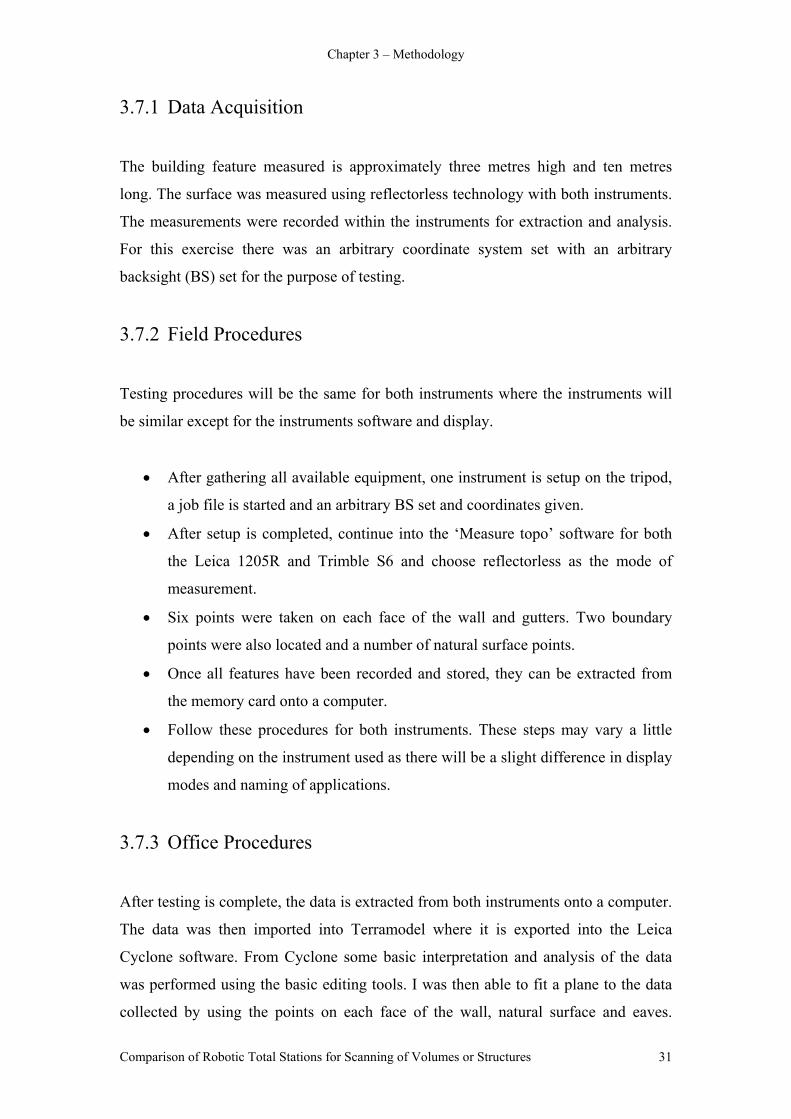
3.7.1 Data Acquisition
The building feature measured is approximately three metres high and ten metres
long. The surface was measured using reflectorless technology with both instruments.
The measurements were recorded within the instruments for extraction and analysis.
For this exercise there was an arbitrary coordinate system set with an arbitrary
backsight (BS) set for the purpose of testing.
3.7.2 Field Procedures
Testing procedures will be the same for both instruments where the instruments will
be similar except for the instruments software and display.
• After gathering all available equipment, one instrument is setup on the tripod,
a job file is started and an arbitrary BS set and coordinates given.
• After setup is completed, continue into the ‘Measure topo’ software for both
the Leica 1205R and Trimble S6 and choose reflectorless as the mode of
measurement.
• Six points were taken on each face of the wall and gutters. Two boundary
points were also located and a number of natural surface points.
• Once all features have been recorded and stored, they can be extracted from
the memory card onto a computer.
• Follow these procedures for both instruments. These steps may vary a little
depending on the instrument used as there will be a slight difference in display
modes and naming of applications.
3.7.3 Office Procedures
After testing is complete, the data is extracted from both instruments onto a computer.
The data was then imported into Terramodel where it is exported into the Leica
Cyclone software. From Cyclone some basic interpretation and analysis of the data
was performed using the basic editing tools. I was then able to fit a plane to the data
collected by using the points on each face of the wall, natural surface and eaves.
Comparison of Robotic Total Stations for Scanning of Volumes or Structures 31
Chapter 3 – Methodology
Comparison of Robotic Total Stations for Scanning of Volumes or Structures 32
Further interrogation of the data was conducted to analyse some results from using the
planes to measure distances and not discrete points. Further analysis was also
conducted using Terramodel to see if 2D based software could produce similar
results. The chainage and offset report was used to analyse the offsets from the
cadastral boundary to the encroaching building face.
3.8 Summary: Chapter 3
In summary this chapter discussed the testing sites, data acquisition and also the office
and field procedures for each of my test designs. To achieve an accurate comparison
between instruments each type of test had to be set on the same coordinate system. It
also allowed the general surveyor to gain an understanding of what limitations his or
her equipment may offer. The methodology of these three test designs are a
replication of my actual procedures and methods used while testing. The following
chapter will discuss the results gathered from this methodology.
Chapter 4 – Results and Analysis
Chapter 4 – Results and Analysis
4.1 Introduction
The objective of this chapter is to present the results from all test designs undertaken
in the methodology. The methodology chapter discussed the appropriate procedures
for all test designs and the comparisons between both instruments. The results from
the tests include the comparisons between the Trimble S6 and Leica 1205R over
various test designs. Each test design compared the instruments for both accuracy and
performance. The results will include the data recorded and a short paragraph
explaining the results obtained.
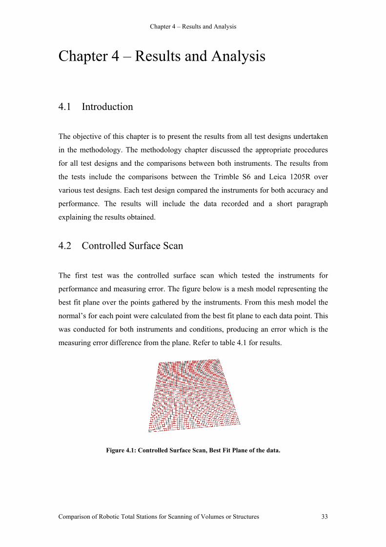
4.2 Controlled Surface Scan
The first test was the controlled surface scan which tested the instruments for
performance and measuring error. The figure below is a mesh model representing the
best fit plane over the points gathered by the instruments. From this mesh model the
normal’s for each point were calculated from the best fit plane to each data point. This
was conducted for both instruments and conditions, producing an error which is the
measuring error difference from the plane. Refer to table 4.1 for results.
Figure 4.1: Controlled Surface Scan, Best Fit Plane of the data.
Comparison of Robotic Total Stations for Scanning of Volumes or Structures 33

Chapter 4 – Results and Analysis
4.2.1 Results Table 4.1: Comparison between instruments.
Instrument Trimble S6 Leica 1205R
Surface Dry Wall Wet Wall Dry Wall Wet Wall
Temperature 20° 20° 20° 20°
Completion Time 4:42 5:32 5:03 5:30
Points collected 124 124 109 109
1 point / second 1/2.1 1/2.6 1/2.7 1/2.9
Mean (m) 0.00037 0.00035 0.00041 0.00035
Standard Deviation (m) 0.00027 0.00026 0.00027 0.00025
% error, (0.250 area) > 1% > 1% > 1% > 1%
4.2.2 Analysis
The results concluded what was expected from the data gathered. The mean deviation
from the plane averaged 0.38 of a millimetre. As the standard deviation was 0.27 of a
millimetre difference from the mean. The percentage error calculated to less than a
percent over the area. These calculations were performed using a least squares macro
using Microsoft Excel. The macro was checked by using the long hand method of
least squares which returned the same results. An interesting observation was the
points collected per second increased as the scanning conditions went from a dry
surface to a wet surface; however the accuracy remained the same. I found the
processing time very quick and easy with both instruments.
4.3 Volumetric Scan
4.3.1 Results
Preliminary setup for the volumetric test site established the ground marks and
coordinate system for each station. Station 1 was given arbitrary coordinates and
reduced level (RL) while station 2 coordinates were calculated and a level run was
performed between the two stations.
Comparison of Robotic Total Stations for Scanning of Volumes or Structures 34
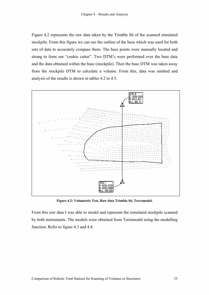
Chapter 4 – Results and Analysis
Figure 4.2 represents the raw data taken by the Trimble S6 of the scanned simulated
stockpile. From this figure we can see the outline of the base which was used for both
sets of data to accurately compare them. The base points were manually located and
strung to form our “cookie cutter”. Two DTM’s were performed over the base data
and the data obtained within the base (stockpile). Then the base DTM was taken away
from the stockpile DTM to calculate a volume. From this, data was omitted and
analysis of the results is shown in tables 4.2 to 4.5.
Figure 4.2: Volumetric Test, Raw data Trimble S6, Terramodel.
From this raw data I was able to model and represent the simulated stockpile scanned
by both instruments. The models were obtained from Terramodel using the modelling
function. Refer to figure 4.3 and 4.4.
Comparison of Robotic Total Stations for Scanning of Volumes or Structures 35
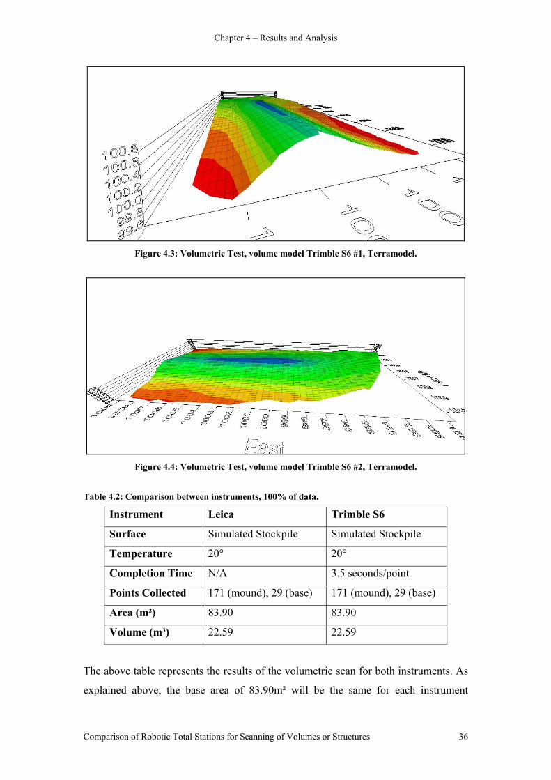
Chapter 4 – Results and Analysis
Figure 4.3: Volumetric Test, volume model Trimble S6 #1, Terramodel.
Figure 4.4: Volumetric Test, volume model Trimble S6 #2, Terramodel.
Table 4.2: Comparison between instruments, 100% of data.
Instrument Leica Trimble S6
Surface Simulated Stockpile Simulated Stockpile
Temperature 20° 20°
Completion Time N/A 3.5 seconds/point
Points Collected 171 (mound), 29 (base) 171 (mound), 29 (base)
Area (m²) 83.90 83.90
Volume (m³) 22.59 22.59
The above table represents the results of the volumetric scan for both instruments. As
explained above, the base area of 83.90m² will be the same for each instrument
Comparison of Robotic Total Stations for Scanning of Volumes or Structures 36
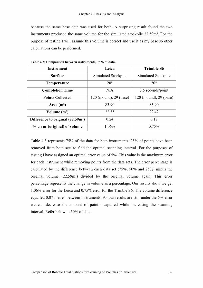
Chapter 4 – Results and Analysis
because the same base data was used for both. A surprising result found the two
instruments produced the same volume for the simulated stockpile 22.59m³. For the
purpose of testing I will assume this volume is correct and use it as my base so other
calculations can be performed.
Table 4.3: Comparison between instruments, 75% of data.
Instrument Leica Trimble S6
Surface Simulated Stockpile Simulated Stockpile
Temperature 20° 20°
Completion Time N/A 3.5 seconds/point
Points Collected 120 (mound), 29 (base) 120 (mound), 29 (base)
Area (m²) 83.90 83.90
Volume (m³) 22.35 22.42
Difference to original (22.59m³) 0.24 0.17
% error (original) of volume 1.06% 0.75%
Table 4.3 represents 75% of the data for both instruments. 25% of points have been
removed from both sets to find the optimal scanning interval. For the purposes of
testing I have assigned an optimal error value of 5%. This value is the maximum error
for each instrument while removing points from the data sets. The error percentage is
calculated by the difference between each data set (75%, 50% and 25%) minus the
original volume (22.59m³) divided by the original volume again. This error
percentage represents the change in volume as a percentage. Our results show we get
1.06% error for the Leica and 0.75% error for the Trimble S6. The volume difference
equalled 0.07 metres between instruments. As our results are still under the 5% error
we can decrease the amount of point’s captured while increasing the scanning
interval. Refer below to 50% of data.
Comparison of Robotic Total Stations for Scanning of Volumes or Structures 37
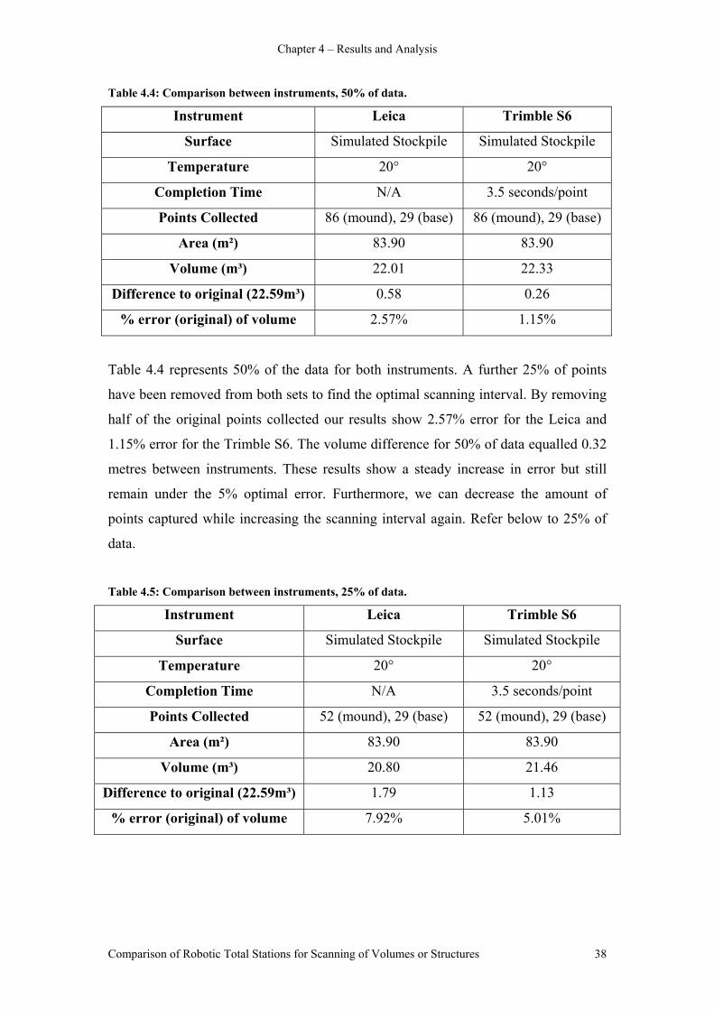
Chapter 4 – Results and Analysis
Table 4.4: Comparison between instruments, 50% of data.
Instrument Leica Trimble S6
Surface Simulated Stockpile Simulated Stockpile
Temperature 20° 20°
Completion Time N/A 3.5 seconds/point
Points Collected 86 (mound), 29 (base) 86 (mound), 29 (base)
Area (m²) 83.90 83.90
Volume (m³) 22.01 22.33
Difference to original (22.59m³) 0.58 0.26
% error (original) of volume 2.57% 1.15%
Table 4.4 represents 50% of the data for both instruments. A further 25% of points
have been removed from both sets to find the optimal scanning interval. By removing
half of the original points collected our results show 2.57% error for the Leica and
1.15% error for the Trimble S6. The volume difference for 50% of data equalled 0.32
metres between instruments. These results show a steady increase in error but still
remain under the 5% optimal error. Furthermore, we can decrease the amount of
points captured while increasing the scanning interval again. Refer below to 25% of
data.
Table 4.5: Comparison between instruments, 25% of data.
Instrument Leica Trimble S6
Surface Simulated Stockpile Simulated Stockpile
Temperature 20° 20°
Completion Time N/A 3.5 seconds/point
Points Collected 52 (mound), 29 (base) 52 (mound), 29 (base)
Area (m²) 83.90 83.90
Volume (m³) 20.80 21.46
Difference to original (22.59m³) 1.79 1.13
% error (original) of volume 7.92% 5.01%
Comparison of Robotic Total Stations for Scanning of Volumes or Structures 38
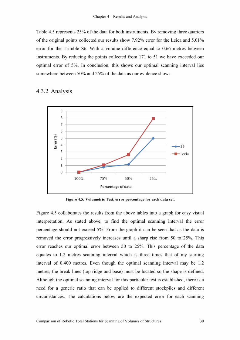
Chapter 4 – Results and Analysis
Table 4.5 represents 25% of the data for both instruments. By removing three quarters
of the original points collected our results show 7.92% error for the Leica and 5.01%
error for the Trimble S6. With a volume difference equal to 0.66 metres between
instruments. By reducing the points collected from 171 to 51 we have exceeded our
optimal error of 5%. In conclusion, this shows our optimal scanning interval lies
somewhere between 50% and 25% of the data as our evidence shows.
4.3.2 Analysis
Figure 4.5: Volumetric Test, error percentage for each data set.
Figure 4.5 collaborates the results from the above tables into a graph for easy visual
interpretation. As stated above, to find the optimal scanning interval the error
percentage should not exceed 5%. From the graph it can be seen that as the data is
removed the error progressively increases until a sharp rise from 50 to 25%. This
error reaches our optimal error between 50 to 25%. This percentage of the data
equates to 1.2 metres scanning interval which is three times that of my starting
interval of 0.400 metres. Even though the optimal scanning interval may be 1.2
metres, the break lines (top ridge and base) must be located so the shape is defined.
Although the optimal scanning interval for this particular test is established, there is a
need for a generic ratio that can be applied to different stockpiles and different
circumstances. The calculations below are the expected error for each scanning
Comparison of Robotic Total Stations for Scanning of Volumes or Structures 39
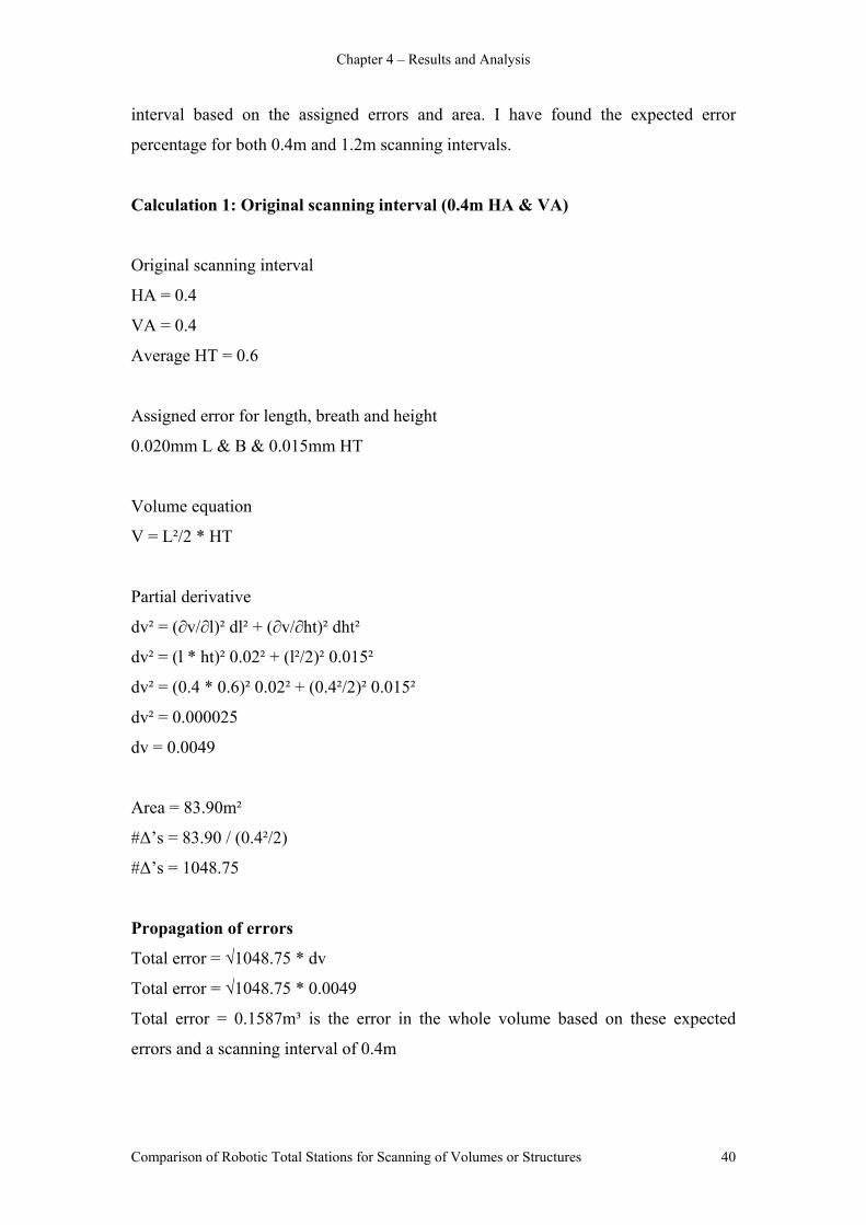
Chapter 4 – Results and Analysis
interval based on the assigned errors and area. I have found the expected error
percentage for both 0.4m and 1.2m scanning intervals.
Calculation 1: Original scanning interval (0.4m HA & VA)
Original scanning interval
HA = 0.4
VA = 0.4
Average HT = 0.6
Assigned error for length, breath and height
0.020mm L & B & 0.015mm HT
Volume equation
V = L²/2 * HT
Partial derivative
dv² = (∂v/∂l)² dl² + (∂v/∂ht)² dht²
dv² = (l * ht)² 0.02² + (l²/2)² 0.015²
dv² = (0.4 * 0.6)² 0.02² + (0.4²/2)² 0.015²
dv² = 0.000025
dv = 0.0049
Area = 83.90m²
#Δ’s = 83.90 / (0.4²/2)
#Δ’s = 1048.75
Propagation of errors
Total error = √1048.75 * dv
Total error = √1048.75 * 0.0049
Total error = 0.1587m³ is the error in the whole volume based on these expected
errors and a scanning interval of 0.4m
Comparison of Robotic Total Stations for Scanning of Volumes or Structures 40

Chapter 4 – Results and Analysis
Percentage error
Area = 83.90m³
Error = 0.1587 / 83.90
Error = 0.19%
This is the expected error percentage based on my original scanning interval of 0.4m
HA and VA. This error is less than one percent, suggesting the scanning interval may
be too small. By increasing the scanning interval I can reduce a number of factors and
still produce an accurate error percentage.
Calculation 2: Adjusted scanning interval (1.2m HA & VA)
Optimal scanning interval
HA = 1.2
VA = 1.2
Average HT = 0.6
Assigned error for length, breath and height
0.020mm L & B & 0.015mm HT
Volume equation
V = L²/2 * HT
Partial derivative
dv² = (∂v/∂l)² dl² + (∂v/∂ht)² dht²
dv² = (l * ht)² 0.02² + (l²/2)² 0.015²
dv² = (1.2 * 0.6)² 0.02² + (1.2²/2)² 0.015²
dv² = 0.00032
dv = 0.018
Area = 83.90m²
#Δ’s = 83.90 / (1.2²/2)
Δ’s = 116.53
Comparison of Robotic Total Stations for Scanning of Volumes or Structures 41

Chapter 4 – Results and Analysis
Propagation of errors
Total error = √116.53 * dv
Total error = √116.53 * 0.018
Total error = 1.4483m³ is the error in the whole volume based on these expected
errors and a scanning interval of 1.2m
Percentage error
Area = 83.90m³
Error = 1.4483 / 83.90
Error = 1.73%
By increasing the scanning interval to 1.2m HA and VA the error has increased to just
below 2%. Based on this adjusted scanning interval the error percentage is still small
but has increased significantly compared to the original of less than 1%.
4.4 Encroachment Testing
The encroachment test was conducted to establish correct measuring procedures,
reflectorless limitation and if 3D models are better than the 2D plans that are currently
used to portray encroachments. Once again a preliminary setup of the encroachment
test site established the ground marks and coordinate system for each station. Station
1 was given arbitrary coordinates and RL while station 2 coordinates were calculated
and a level run was performed between the two stations.
4.4.1 Results
Measurements were taken on all faces of the building, natural surface and two marks
on the ground representing the cadastral boundary. Figure 4.6 represents a 2D model
of the data. Traditionally this is how the data is represented and displayed. As this
figure is only 2D there is actually three slightly different points at each section of the
wall. This is used to represent the vertical orientation of the wall. I have done this
because the wall might be leaning or bowed and by taking points at the bottom,
middle and towards the top I can model the true vertical orientation of the wall.
Comparison of Robotic Total Stations for Scanning of Volumes or Structures 42
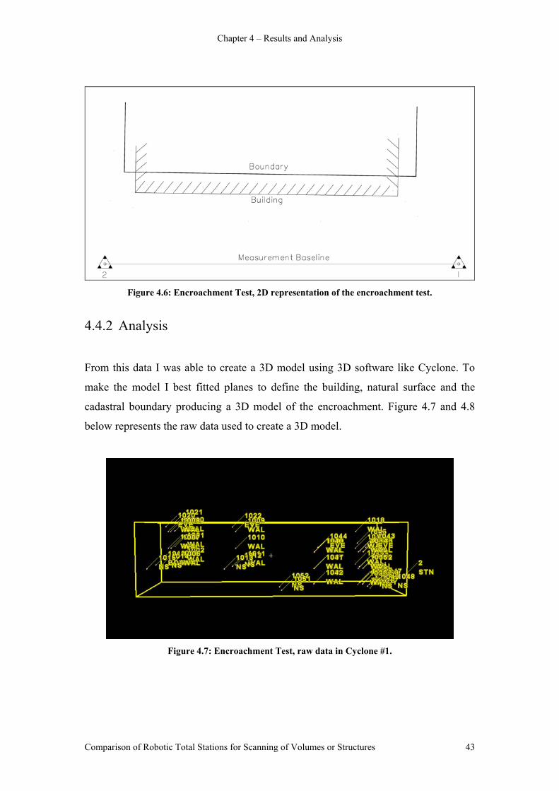
Chapter 4 – Results and Analysis
Figure 4.6: Encroachment Test, 2D representation of the encroachment test.
4.4.2 Analysis
From this data I was able to create a 3D model using 3D software like Cyclone. To
make the model I best fitted planes to define the building, natural surface and the
cadastral boundary producing a 3D model of the encroachment. Figure 4.7 and 4.8
below represents the raw data used to create a 3D model.
Figure 4.7: Encroachment Test, raw data in Cyclone #1.
Comparison of Robotic Total Stations for Scanning of Volumes or Structures 43

Chapter 4 – Results and Analysis
Figure 4.8: Encroachment Test, raw data in Cyclone #2.
Figure 4.9 represents how planes can be used to show the points gathered. The model
shows the green plane used to represent the cadastral boundary while the other planes
in grey colour represent the building encroachment. Analysis of the planes proved to
be difficult as the software would not allow me to perform calculations from plane to
plane. This software has the potential to analyse any location on the model to find a
distance, area, volume or even the sinuosity of an object.
Due to the 3D modeling capabilities of Leica Cyclone and my inexperience in the
software I was unable to gather any measurements. Measuring from point to point is
relativity simple and does not require a 3D model. However, for this test my objective
was to measure information from one plane to another.
Figure 4.9: Encroachment Test, 3D representation of the encroachment test.
Comparison of Robotic Total Stations for Scanning of Volumes or Structures 44

Chapter 4 – Results and Analysis
Comparison of Robotic Total Stations for Scanning of Volumes or Structures 45
After further discussions with my supervisor we thought it would be good to conduct
some additional research into the capabilities of Terramodel. After analysing the data
I was able to produce a report showing the chainage and offset from the cadastral
boundary to the points on the wall, eaves and natural surface. Below is a section of
that report, which shows the chainage and offset distance from the alignment of the
cadastral boundary to each point. For the full report refer to appendix H - chainage
and offset report.
ALIGNMENT REPORT Alignment Name: Free Pts Point Number Description Chainage Easting Northing Elevation Offset -------------------------------------------------------------------------------- 1004 WAL 2.658 996.670 1004.249 101.389 0.009 1007 WAL 3.093 996.425 1003.906 101.391 0.004 1008 WAL 7.681 996.422 1003.909 102.591 4.588 1011 WAL 8.009 991.829 1003.973 100.190 0.322 1012 NS 16.916 992.071 1003.760 100.101 8.908
Figure 4.10: Encroachment Test, Chainage and Offset Report Terramodel.
4.4 Summary: Chapter 4
In summary this chapter has collectively included all results from each of the three
test designs. The controlled surface scan produced as expected results and showed the
capabilities of the scanning function. The volumetric test also showed how it can
provide surveyors with a useful tool in real scenario surveying. From the results an
optimal scanning interval was established for my scan and calculations of the
expected errors were performed. Lastly, the encroachment test also showed how
reflectorless technology may be used to remotely sense data that is inaccessible and
how 3D models may be used to represent spatial information.

Chapter 5 Discussion
Chapter 5 – Discussion
5.1 Introduction
This chapter will discuss the results found during the test design stage. I will discuss
some important features found during the designs and the correct methods for
conducting them. There will also be discussion of some results found by other
students that performed more in depth testing on some sections of my designs.
5.2 Discussion
At the start of this year I was not aware that total stations had integrated laser
scanning capabilities into their instruments. I was aware that reflectorless technology
was relativity new and the limitations of this technology have not been fully
publicised. Throughout the progression of this project I have realised the full potential
these instruments have. Their usefulness and applications in the surveying industry is
advantageous and notable.
5.2.1 Controlled Surface Scan
The controlled surface scan was a basic test to analyse and compare both instruments
against one another and the manufacturer’s specifications. From my testing the results
that were found was what was to be expected. The errors were very small and
insignificant (0.00027m). The manufacturers claim a 2mm + 2ppm error for distances
measured less than 500 metres. The object I measured to was 5 metres away from the
instrument, so it was expected that there would be an error in the measuring device
and that error would be very small over this distance. Further comparison could have
been done to test the error at different intervals further away from the object. After
listening to another student’s presentation he concluded that the error did increase and
that there was beam divergence the further away he got. An issue I had concerns with
was the laser dot in accordance with the optical cross hairs in the total station. After
Comparison of Robotic Total Stations for Scanning of Volumes or Structures 46

Chapter 5 Discussion
talking to another student doing a similar project it was realised that he had came to
the same conclusion which was that they were not in accordance with one another.
Care must be taken when measuring to features to always try and use the cross hairs
within the optical devices as this has be calibrated (in most cases).
The next comparison was between both instruments and as expected again there was
no difference between each instrument where they produced roughly the same error.
From this I could not distinguish between them as they are in error by roughly the
same factor. It is important to note that although the instruments are made by different
manufacturers, they both have similar characteristics. They are both have magnetic
driven systems, have similar specifications and similar capabilities. However, the
Trimble S6 uses a pulsed based mode of measurement and the Leica uses a phase
based mode of measurement. From my results I cannot distinguish between the modes
of measurement as there are no differences in error. Further testing would be required
to ascertain this information.
Last was the comparison of both instruments over the different conditions. As
expected again there was very small error difference from a dry surface to a wet
surface. However one thing I did find different was the change in recording time. The
manufacturers specify 3 – 6 seconds a point less than 500 metres. When performing
my tests I achieved one point every 2.1 seconds on a dry surface and 2.6 seconds on a
wet surface with the Trimble S6. This increase is consistent with both instruments
which suggest that water droplets on a walls surface will delay the return signal.
As I was experimenting with the instrument I noticed that they did not reflect from
certain objects. These features included a glass panel on a door and a light covering
made of rough plastic. I found that there was no return signal when measuring to the
light covering which suggests that there was scattering and absorption contributing to
this. When the instrument measured to the glass on the door it sounded like a faint
signal was being returned as the instrument would beep once compared to no beep for
the light covering. The instrument tried to measure this particular point up to 4 times
before it disregarded it. Measuring to any feature that affects the EMR is difficult to
rely on the results, care must be taken when recording information to features that
may alter the signal.
Comparison of Robotic Total Stations for Scanning of Volumes or Structures 47

Chapter 5 Discussion
While the error at close distances is small, correct measuring producers must still be
used. As discussed in the literature review section 2.5.2, a laser beam may not
necessarily be measuring what you are pointing to. The correct procedures for
measuring building corners are to measure the faces of the building and intersect them
in the office to get the corner. This will eliminate the errors of measuring to external
or internal corners. Another important factor to consider when measuring features is
the angle of incidence from the instrument to the feature being measured. In my test I
was not affected by this as I was perpendicular to my testing object. When conversing
with my peers it became apparent that one student tested the affects of angle
incidences and found that as the angle became acute there was no reflection from the
object. This was due to the acute angle deflecting the laser beam in an opposite
direction rather than reflecting back to the instrument.
5.2.2 Volumetric Scan
Workplace Health and Safety stops surveyors from venturing onto unsafe areas
whether it be a stockpile, high wall in a mine or high places like a building feature.
These issues along with accurately taking measurements can cause problems.
Accurately measuring volumes is difficult; this is mostly due to the varying and
undulating topology of the surface. This results in an approximated volume based on
the measurements taken. Due to laser scanning technology, a surface can be scanned
at less than 50mm intervals, producing a high 3D level of detail. From this model a
volume can be calculated by taking the scanned surface away from a base level
(usually natural surface) which leaves the volume.
So the question is, will taking more points at closer scanning intervals produce a
better estimated value than fewer points at larger intervals? From my test I was able to
establish this relationship and find the optimal scanning interval that would still
produce an accurate value. Accuracy raises another question of how accurate does the
volume need to be? Mines have the perspective that accuracy is not an important trait.
This is misconceived in some contexts as the monitoring of a wall to find if it will
Comparison of Robotic Total Stations for Scanning of Volumes or Structures 48
Chapter 5 Discussion
collapse or the volumetric calculation of a material that is exchanged for money is
very important and must be accurate.
Over the past 15 years the method of measuring volumes has evolved from recording
points with a prism & pole to reflectorless and now laser scanning. Reflectorless has
removed the risk of unsafe procedures by remotely sensing points of data from a safe
position. In the last ten years laser scanning units have been introduced to surveyors.
The laser scanning unit could only perform scans and was very expensive. This
system is typically used in the mines as they can afford it and they have the need for
gathering a lot of point’s inaccessible areas. Technology has now gone one step
further and incorporated scanning into total stations. This results in the everyday
surveyor still having the ability to perform general surveying applications, however
now having the ability to perform scans on a surface.
From the undertaking of the research involved in writing this dissertation I learnt a lot
about what the software can do and the correct procedures for performing them. As I
have stated previously total station scanning is relatively new and there has been
limited testing on this technology. I believe incorporating scanning capabilities into a
total station is the way to the future in surveying equipment. The introduction of a
scanning function has not altered the physical instrument or internal components.
There are no disadvantages by including the scanning function into a total station
besides the capabilities of the scanner & drafting software, “but something is better
than nothing”. Below is a list of the advantages and disadvantages of laser scanning.
Advantages of a total station scanning instrument:
• A single total station instrument is cheaper compared to that of a single laser
scanning unit.
• A total station instrument has more capabilities than that of a single laser
scanning unit (can still perform traditional traversing etc).
• The data captured is compatible with current surveying software (Terramodel,
AutoCAD etc).
Comparison of Robotic Total Stations for Scanning of Volumes or Structures 49

Chapter 5 Discussion
• The scanning function is useful for the everyday surveyor that would only
perform a limited amount of scans a year.
• Ability to record information that was not accessible before due to safety
issues.
• It is a single complete unit, as the external and internal characteristics of the
instrument have not changed compared to a scanner which needs a laptop,
external battery, etc).
• Requires only one field technician.
• Semi-automated stand alone system (set it up and let it scan).
Disadvantages of a total station scanning instrument:
• The 3D software capabilities are limited.
• Cannot view in real time.
• A laser scanning unit can record up to 50,000 points a second, while a total
station records one point every 3 seconds.
• The scanning capabilities are only basic compared to that of a laser scanning
unit.
In my opinion the advantages of including a laser scanning function into a total station
outweigh the disadvantages. As technology continues to evolve the disadvantages
listed above will be refined and tuned which will enhance the technology. Like all
technology it will become quicker, the software capabilities will become better and
the ability to connect up to a laptop and get real time information will be available
within the near distant future.
The main purpose of this test was to scan a simulated stockpile with both instruments
to find the optimal scanning interval. Due to some problems with the Leica’s scanning
software I was unable to perform a scan but instead recorded reflectorless
measurements at my discretion. The Trimble S6 performed the scan very well, with
no problems and all the points captured. The data processing stage was also very
quick and easy as the data was extracted straight into Terramodel where I could
investigate it. Besides the fact that I could not perform a scan with the Leica the data
Comparison of Robotic Total Stations for Scanning of Volumes or Structures 50

Chapter 5 Discussion
processing was straight forward. Once the data was imported into Terramodel I
calculated a volume for both sets of data. From this I proceeded to remove 25% of the
data and calculated a volume. I continued this formula to find a result for 50% and
75% of the data removed to calculate the percentage of change. Removing 25% and
50% of data only equated to a 1% change with the Trimble and roughly a 3% change
with the Leica. A noticeable change occurred when 75% of data was removed where
the Trimble went to 5% and the Leica 8%. After discussion with my supervisor we
decided that the error would become significant once the data reached 5%. This would
be our optimal scanning interval. The initial scanning interval was 0.400m
horizontally and 0.400m vertically.
By adopting only 25% of the original data for this test, the scanning interval was three
times that of my starting interval. The optimal interval for my particular test was 1.2
metres. It is important to note the break lines, those being the top ridge and base of the
feature being scanned. If in my situation I did not gather enough data along these
break lines then I would not be confident that the shape of my stockpile would be
truly represented. This would lead to a poorly estimated volume as areas of the
stockpile would be generalised because of significant data and not the true shape of
the undulating surface.
When comparing the error percentage between both instruments, the Trimble S6
shows the least amount of error deviation compared to the Leica at all three changes
(75%, 50% and 25%). Additional analysis of the instruments led me to investigate the
apparent variations of points over the simulated stockpile. The Trimble S6 data
pattern is uniform and evenly spread across most of the stockpile. This is expected as
the instrument controls the pointing of the instrument after the user has defined the
parameters as compared to the Leica where reflectorless measurements were taken at
my discretion over the simulated stockpile. Currently this is standard practice as most
surveying companies gather points the traditional way by using a pole and prism
which see’s each point reliant on the technician’s discretion. Figure 4.5 would suggest
a uniform and machine guided pointing will produce a more accurate measurement.
However, this may not be the case. When performing a scan the instrument will only
record points on its grid section. The instrument will not detect sudden variations in
the surface, whereas by using the traditional method the field technician can locate the
Comparison of Robotic Total Stations for Scanning of Volumes or Structures 51
Chapter 5 Discussion
sudden variations. This all comes back down to the scanning interval. A larger
scanning interval will generalise the surface more and miss certain information if the
interval is too large. Compared to small scanning intervals this will better estimate the
surface as it will locate more points and produce a more accurate model of the
surface, essentially producing more accurate results. But will measuring at smaller
intervals produce a more accurate answer than larger intervals and greater
generalization of the surface? Figure 4.5 suggests that a smaller scanning interval
does produce more accurate results. This is because as the data was removed the error
increased. From this figure it also suggests that the uniform scanning pattern of the
Trimble S6 also produced more accurate results than randomly locating points with
the Leica. Because the S6 scan is uniform, at set gridlines and small scanning
interval, the level of detail at critical locations is captured. By having a uniform scan
over the simulated stockpile the error was reduced compared to that of randomly
locating points at my discretion. This strengthened the idea that scanning will produce
a more accurate answer.
Manual calculations were carried out to find the expected error for 0.4m and 1.2m
scanning intervals. These calculations were done by using partial derivative and
propagation of errors methods. The results found for 0.4m scanning interval the error
equated to less than 1% for the total area. By increasing the scanning interval to 1.2m
the error was just under 2% for the total area. These errors are based on the whole
volume and are influenced by the assigned errors and scanning interval.
As reflectorless does not require anything to reflect, its measurements are taken to the
first thing that the laser comes in contact with, which in this case is the grass. But
when recording information, traditionally we use a prism and pole and when placing
the pole into the ground it would be 30 to 60mm under the surface of the grass. This
raises another problem of what is the surface we are trying to measure. Is it just below
the dirt, dirt level or grass level? In most cases this difference will not matter, but
surveyors need to be mindful of what incident energy is reflecting from.
In summary as the data was extracted the error percentage increased. I established that
this error percentage should not exceed 5% as the error would then become
significant. By removing data I could continue to calculate my error percentage until I
Comparison of Robotic Total Stations for Scanning of Volumes or Structures 52
Chapter 5 Discussion
reached the 5%. This percentage exceeded my optimal error between 50 and 25% of
the data. This equated to 3 times my starting interval of 0.4m to 1.2m. By using a
1.2m scanning interval on my initial scan I could have reduced my scanning time,
data processing, storage and still maintained an accurate volume.
5.2.3 Encroachment Testing
The encroachment testing was conducted to establish correct measuring procedures,
reflectorless limitations, capabilities of the software and if a 3D model of the
encroachment is better than a 2D plan which are currently used to portray
encroachments. The design had to replicate a building encroachment situation. With
the use of both instruments, reflectorless measurements were taken to the building
walls, eaves, natural surface and two marks representing the cadastral boundary. The
aim of this data was to create a 3D model of the encroachment by fitting planes to the
points captured. From this model I was expecting to obtain measurements from plane
to plane to calculate distances, volumes and areas etc. The second analysis was to use
Terramodel to calculate a chainage and offset report from the cadastral boundary to
each point on the wall.
Due to some software capabilities and my inexperience in the software I was not able
to record any measurement from plane to plane. The theory behind using a 3D model
was to use planes instead of discrete points to perform calculations. This would
provide better analysis of information anywhere on the model thereby achieving
greater accuracy for calculating volumes and distances at any location on the model.
After some manipulation with the data structure I was able to import it into the Leica
Cyclone software. From this I fitted planes between points and produced a 3D model.
However, my analysis had come to a halt as I could not perform my intended
calculations. The software would only let me perform measurements from point to
point which I can do in a normal software package. On a positive note, the 3D
software did make it easier to visualise the model and select points.
Comparison of Robotic Total Stations for Scanning of Volumes or Structures 53
Chapter 5 Discussion
Figure 4.9 shows how planes can be used to show the shape of a building and the
cadastral boundary. This model provides a greater level of detail and information
compared to traditional 2D plans that are currently used to represent encroachments.
Referring to Appendix E which shows the right hand side of the survey plan where
there are two garden sheds encroaching. These are shown as a single black line over
the boundary with an annotation of 0.9 over. In 4.9 we can see precisely where the
cadastral boundary slices through the building. With this model the ability to annotate
these lines and planes to include areas, volumes and distances would be useful. As
modeling software continues to evolve I expect calculations from plane to plane and
other functions will become available.
Looking at a more complex encroachment like the Gabba stadium in Brisbane there
are beams, braces and structural features all throughout the encroachment. Because
the encroachment is not fully enclosed like my example above, the impression of the
encroachment may be misunderstood to be that the whole area/volume under this is
encroaching. But in fact only a small volume of features are encroaching. In this
situation a single 2D plan does not do justice to fully show the encroachment. Only
showing the furtherest extended structural edging may be ok to show the extent but
should provide more information. If there was a 3D scanned drawing of the complex
encroachment then a whole range of analysis may be performed like calculations of
clearances, structural design, improvements and from the surveying side the
encroachment itself represented in 3D. When compared to the 2D representation of
the encroachment we could not acquire this information. This method of
representation also raises problems of software capabilities, failure to produce a hard
copy plan and the amount of detail actually required for the encroachment.
The second method of analysis was producing a report showing the chainages and
offsets from the cadastral boundary to each feature using Terramodel. The process
was to assign an alignment to the cadastral boundary. From this alignment a report
was done which calculated the chainage along the alignment from the start and the
offset from my alignments to each feature. This method worked well and the report
was very quick. But in the situation where the building encroachment completely
obstructs a clear view from one boundary corner to the other, there is a problem of
knowing if you are on that alignment to measure the offset. When creating this
Comparison of Robotic Total Stations for Scanning of Volumes or Structures 54

Chapter 5 Discussion
alignment there is no vertical component. I recorded three measurements at different
heights above each other to show the vertical orientation. This method of interpolating
the chainage and offset is difficult to measure in the field. This method may be useful
not to produce a report but to transfer data. Instead of producing a report, the
information can be exported as a text file. The text file would contain point numbers,
description, chainage, offsets and elevation. Form this text file the data can imported
into Terramodel, AutoCAD or a hardcopy plan. This may be an alternative approach
for lodging encroachment information.
Finally, I would like to mention the electronic lodgment of survey related information.
Currently, most encroachments are represented on 2D plans refer to appendix I. Most
encroachments are represented by the most extended feature encroaching on the
neighbouring land whether it is the crown or private land. In the case that the
encroachment was quite complex and a greater detail of information is required then
how is this to be displayed on a 2D plan? At the moment there is no provision for
lodging electronic plans. Currently in progress is a system of electronic lodgment of
surveying data (survey plans). Electronic lodgment of survey information may
enhance the level of information provided to clients, developers and other surveyors.
In the case mentioned above about the Gabba stadium in Brisbane, an electronic
lodgment of the survey scan or reflectorless measurements would provide people with
more information. The plan may be sent electronically at a fee to the person
requesting the information where they can use a 3D modeling software to interrogate
and query the information. This would save costs and time because the current 2D
plan does not show any extra information and a 3D plan can include information
about the beams, braces, size and shape of features which can be stored on a single
electronic drawing.
5.3 Summary: Chapter 5
This chapter covered an in-depth discussion of all three test deigns, their results,
performance and conclusions. Both instruments performed to the manufacturers
specification over all three tests. This chapter also covered some conclusions sought
from other peers about what they have found during their testing. The discussions not
Comparison of Robotic Total Stations for Scanning of Volumes or Structures 55

Chapter 5 Discussion
Comparison of Robotic Total Stations for Scanning of Volumes or Structures 56
only spoke about the advantages but more importantly the disadvantages of the
instruments, software and their abilities. The next chapter will discuss my
recommendations and a final conclusion about the equipment and objectives for this
project.
Chapter 6 Recommendations & Conclusion
Chapter 6 – Recommendations &
Conclusion
6.1 Introduction
This chapter will outline some recommendations that may be of assistance to users in
regards to total station laser scanning and the establishment of guidelines that industry
companies can develop. To conclude there will be a summary of the final outcomes of
this project and a statement of whether I have achieved the objectives set at the
commencement of this project.
6.2 Recommendations
The Leica 1205R and the Trimble S6 have proven to be very useful tools in surveying
applications. Both instruments have reflectorless technology and laser scanning
functions which have satisfied the three tests that were conducted. However, there are
a number of key features that I would recommend to the manufacturers of these
instruments and also to users. They are:
Polygon scan feature: Both instruments have a number of scan functions built into
the instrument that allows the user to choose the type of scan they want. Some include
rectangle scan and offset scan. The problems with these applications are that they
mainly cater for scanning surfaces that are parallel and perpendicular because that is
how the scan area is defined. Most stockpiles or mounds of dirt are in the shape of a
bell shaped curve or an upside down parabola. So instead of defining a rectangle scan
area over the stockpile, the user could identify the scan area by locating a number of
points along the break lines of the feature and the scan would be contained within this
area. By doing this, a lot of factors may be reduced including the amount of point data
captured, scan time, storage and processing time.
Comparison of Robotic Total Stations for Scanning of Volumes or Structures 57
Chapter 6 Recommendations & Conclusion
Inefficient measuring of non-reflective points: On average it takes a total station
3.5 seconds to record a point. When measuring a non-reflective feature the instrument
will try to record the point up to 4 times before it disregards it and moves to the next
one. When I compared a total station scanning instrument and a laser scanning unit I
found that the laser scanning unit will disregard points if they do not reflect the first
time whereas a total station instrument continues to record the point. This leads to
inefficient measuring of non-reflective points, resulting in time loss. I recommend
including a feature that specifies the number a retries a single point may have if the
point is non-reflective.
Establish guidelines on optimal scanning intervals and expected errors: Most
surveying applications like detail surveys rely on the user’s discretion on optimal
contour intervals and the like. I believe that establishing guidelines on optimal
scanning intervals of different features, shapes and materials would be of great
benefit. This may be utilised as a guide for users because I found that I chose either a
higher spacing interval or lower spacing interval than that of the optimal spacing
interval. This resulted in me recording too much data or not enough data. Guidelines
also need to be established on expected errors for the scanning of grain, soil, rock and
coal etc. Additional information about different material densities can also be
included and applied in the calculation stage to gather a better approximation of
volume.
Encroachments: Currently in Queensland there is no provision for electronic
lodgment of surveying information (survey plans, volumetric plans etc). I believe this
is currently in the process of changing to electronic lodgment of surveying data. By
introducing this new method of lodgment other related information like a 3D model
scans of an encroachment may be attached to the survey plan and lodged as one. This
method would be most beneficial in mining situations where a standard can be
established and information stored about the workings of mines. I personally believe
this is the way of the future as technology is continually evolving and an increasing
amount of information is transferred electronically via computers and the internet.
Comparison of Robotic Total Stations for Scanning of Volumes or Structures 58
Chapter 6 Recommendations & Conclusion
6.2.1 Further Research
This project has covered three areas of testing and analysis involved with reflectorless
technology and laser scanning capabilities. They are controlled surface scan testing,
volumetric testing and encroachment testing. Further research can be conducted over
the three tests designs within this project.
More extensive research may be carried out on my first test, the controlled surface
scan, by measuring and analysing the effects of a wide range of colours, surfaces
(rough or smooth), water, range and materials. As I only touched the basis on most of
these areas, further research would be useful for determining errors in different
applications.
The calculations of volumes are never 100% correct due to the irregularities within
materials. Most volumetric surveying scans are approximated based on the area
between points and not a true model of the varying area. Most of the materials
scanned will contain air pockets or gaps between the materials which when scanned
will over estimate the volume. This is due to the amount of spacing or area between
materials and will also depend on the material measured. For example, a rock may
have bigger gaps or spacing compared to a grain material. Therefore, there is the need
for further research into densities of different materials in determining more accurate
measuring of volumetric features.
My final recommendation is to further the research into the requirements of a
surveyor in an encroachment situation. Research the requirements of accuracy,
information required and the representation of encroachments on survey plans.
Particularly the lodgment of electronic encroachment plans and how they may attach
to a survey plan and lodged in the titles office.
Comparison of Robotic Total Stations for Scanning of Volumes or Structures 59

Chapter 6 Recommendations & Conclusion
Comparison of Robotic Total Stations for Scanning of Volumes or Structures 60
6.3 Conclusion
The reflectorless capabilities of both instruments performed very well with little
difference between the two. However, the scanning capabilities of the Trimble S6
proved to be the better instrument due to its user-friendliness, quick & easy setup of
scans and easy processing of data. The Leica 1205R was still a suitable instrument for
performing scans but it had a difficult to follow display, naming of applications and
took a long time to setup scans.
My supervisor and I set out a number of goals to achieve throughout the fulfillment of
the project. I believe I have covered most of the objectives to a satisfactory standard.
This dissertation covers the research of existing laser scanning technology,
capabilities and specification of both the Trimble S6 and Leica 1205R. It also includes
the three test designs which analysed both instruments for speed, accuracy and
performance on a range of different applications including a simple point comparison,
scans over a simulated stockpile and reflectorless measurement of building features
which were performed under different conditions. These tests were analysed
according to a range of criteria where the implications and results were discussed with
respect to surveying organisations and potential opportunities.
In conclusion, this project compared the laser scanning capabilities and reflectorless
limitation of two robotic total stations for various surveying applications.
Reflectorless and laser scanning capabilities were tested and the fundamental theory
behind the technology was discussed in the literature review. The methods, results and
discussions covered the test designs performed and the outcomes of these tests. This
conclusion spoke about my recommendations, further research and an overview of my
dissertation.
References
References Bourke, P 1989, Equation of a Plane, UWA, viewed 9 May 2009,
http://local.wasp.uwa.edu.au/~pbourke/geometry/planeeq/
Brown, L 2004, Reflectorless Revolution, Point of Beginning, viewed 23 April 2009,
http://www.pobonline.com/Articles/Features/4ffe56559e0f6010VgnVCM100000f932
a8c0
Center for Advanced Spatial technologies n.d., 3d Laser Scanning – How We Do It,
University of Arkansas, viewed 3 May 2009,
http://www.cast.uark.edu/home/research/archaeology-and-historic-
preservation/archaeological-geomatics/archaeological-laser-scanning/archaeological-
laser-scanning-techniques.html
CESCafe 2008, 3D Laser Scanning for Surveying Application, CESCafe Civil
engineering society, IIT Kharagpur, viewed 3 May 2009,
http://www.cesiitkgp.org/CESCafe/index.php/2008/01/21/3d-laser-scanning-for-
surveying-applications/
DeLiberty, T 1999, Energy Interactions with the Atmosphere and at the Surface,
Google, viewed 12 May 2009,
http://www.udel.edu/Geography/DeLiberty/Geog474/energy_interactions.gif
DeLiberty, T 1999, Energy Interactions with the Atmosphere and at the Surface,
Geography 474, viewed 12 May 2009,
http://www.udel.edu/Geography/DeLiberty/Geog474/geog474_energy_interact.html
Department of Environment and Resource Management 2007, Chains, Queensland
Government, viewed 25 April 2009,
http://www.nrw.qld.gov.au/museum/articles_complete/surveying/chains.html
El-Hakim, S Beraldin, J. Remondino, F Picard, M Cournoyer, L Baltsavias, E n.d.,
Using Terrestrial Laser Scanning and Digital Images for 3D Modelling of the
Comparison of Robotic Total Stations for Scanning of Volumes or Structures 61
References
Erechtheion, Acropolis of Athens, Visual Information Technology, National Research
Council, Canada, viewed 3 May 2009,
http://www.photogrammetry.ethz.ch/general/persons/fabio/DMACH08_acropolis.pdf
GIM International 2009, Reflectorless Laser Distance Measurement, GIM
International, viewed 27 April 2009, http://www.gim-
international.com/issues/articles/id417-
Reflectorless_Laser_Distance_Measurement.html
Globe GIS n.d., Electromagnetic Spectrum: Transmittance, Absorptance, and
Reflectance, Globe GIS, viewed 13 May 2009,
http://globegis.blogspot.com/2007/07/this-page-concentrates-on-what-can.html
Google n.d., Background on Spectral Signatures, Google, viewed 10 May 2009,
http://geog.hkbu.edu.hk/virtuallabs/rs/env_backgr_refl.htm
Hoglund, R and Large, P 2005, Direct Reflex EDM Technology for the Surveyor and
Civil Engineer, viewed 15 April 2009,
http://trl.trimble.com/docushare/dsweb/Get/Document-208582/022543-
010D_TrimbleS6_DR_WP_1104_lr.pdf
Knol n.d., 3D laser scanning, Knol: A unit of knowledge, viewed 4 May 2009,
http://knol.google.com/k/paul-oberle/3d-laser-scanner/13av68kkt1k9q/2#
Lammon, T and Jung, R 2005, Trimble S6 with magdrive servo technology, viewed 15
April 2009, http://trl.trimble.com/docushare/dsweb/Get/Document-208581/022543-
100_TrimbleS6_MagDrive_WP_1204_lr.pdf
Leica Geosystems, 2009, Leica TPS1200+ series, viewed 15 April 2009,
http://www.leica-
geosystems.com/downloads123/zz/tps/tps1200/brochures/Leica_TPS1200+_brochure
_en.pdf
Comparison of Robotic Total Stations for Scanning of Volumes or Structures 62
References
Comparison of Robotic Total Stations for Scanning of Volumes or Structures 63
Leica Geosystems 2009, Leica Total Stations, viewed 20 April 2009,
http://www.surveyequipment.com/shop/index.php?main_page=product_info&product
s_id=988
Mather, M 2004, Computer Processing of Remotely-Sensed Images: An Introduction,
John Wiley & Sons, England.
National Research Council Canada 2006, Optical Frequency Comb, National
Research Council Canada, viewed 10 May 2009, http://inms-ienm.nrc-
cnrc.gc.ca/images/research_images/optical_comb/COMBFIG1.gif
South Carolina Department of Natural Resources 2009, Electromagnetic Spectrum,
viewed 16 April 2009, http://www.dnr.sc.gov/ael/personals/pjpb/lecture/spectrum.gif
Strategic Engineering Resources 2009, Laser Scanning Applications, SER, viewed 12
May 2009, http://ser-corporate.com/images/scan.gif
Trimble, 2009, Trimble S6 Data sheet, viewed 15 April 2009,
http://trl.trimble.com/docushare/dsweb/Get/Document-208580/022543-
098H_TrimbleS6_DS_0707_lr.pdf
University of Minnesota n.d., Electromagnetic spectrum, with frequency and
wavelength properties, viewed 16 April 2009,
http://www.lcse.umn.edu/specs/labs/images/spectrum.gif
Wikipedia n.da., Phase Shift, viewed 15 April 2009,
http://en.wikipedia.org/wiki/File:Phase_shift.svg
Wikipedia n.db., Diffuse Reflection, viewed 15 April 2009,
http://en.wikipedia.org/wiki/File:Diffuse_reflection.PNG
Wikipedia n.dc., Reflection Angles, viewed 15 April 2009,
http://en.wikipedia.org/wiki/File:Reflection_angles.svg

Appendices
Appendices Appendix A – Project Specification
Comparison of Robotic Total Stations for Scanning of Volumes or Structures 64
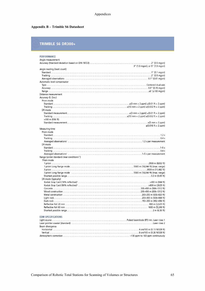
Appendices
Appendix B – Trimble S6 Datasheet
Comparison of Robotic Total Stations for Scanning of Volumes or Structures 65
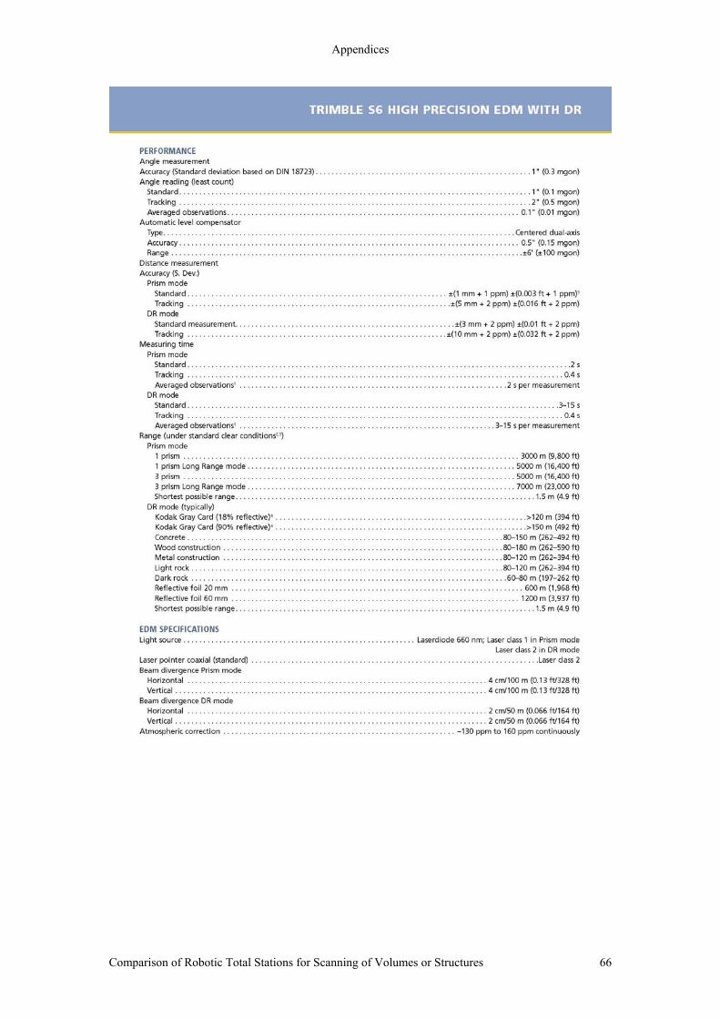
Appendices
Comparison of Robotic Total Stations for Scanning of Volumes or Structures 66

Appendices
Appendix C – Leica TPS1200+ Datasheet
Comparison of Robotic Total Stations for Scanning of Volumes or Structures 67
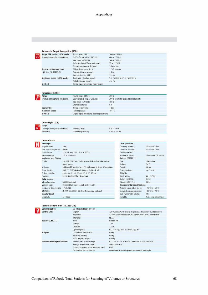
Appendices
Comparison of Robotic Total Stations for Scanning of Volumes or Structures 68

Appendices
Appendix D – S6 Dry Conditions.
Point Easting Northing RL Normal ABS Average Standard
Dev 2000 995.267 5006.196 100.426 0.0007 0.0007 0.00037 0.000272001 995.266 5006.197 100.426 -0.0005 0.0005 2002 995.443 5006.661 100.44 -0.0004 0.0004 2003 995.269 5006.202 99.926 0.0006 0.0006 2004 995.284 5006.243 100.427 -0.0001 0.0001 2005 995.302 5006.29 100.429 0.0000 0.0000 2006 995.32 5006.336 100.43 0.0004 0.0004 2007 995.338 5006.383 100.432 0.0005 0.0005 2008 995.355 5006.43 100.433 -0.0004 0.0004 2009 995.374 5006.476 100.435 0.0010 0.0010 2010 995.391 5006.524 100.436 -0.0002 0.0002 2011 995.409 5006.57 100.438 0.0002 0.0002 2012 995.427 5006.616 100.439 0.0006 0.0006 2013 995.443 5006.661 100.44 -0.0004 0.0004 2014 995.444 5006.662 100.39 0.0002 0.0002 2015 995.427 5006.619 100.389 -0.0004 0.0004 2016 995.409 5006.572 100.388 -0.0005 0.0005 2017 995.391 5006.525 100.386 -0.0006 0.0006 2018 995.374 5006.478 100.385 0.0003 0.0003 2019 995.356 5006.431 100.383 0.0002 0.0002 2020 995.338 5006.385 100.382 -0.0002 0.0002 2021 995.32 5006.338 100.38 -0.0003 0.0003 2022 995.303 5006.291 100.379 0.0006 0.0006 2023 995.285 5006.245 100.377 0.0001 0.0001 2024 995.267 5006.198 100.376 0.0000 0.0000 2025 995.267 5006.2 100.326 -0.0006 0.0006 2026 995.285 5006.246 100.327 -0.0002 0.0002 2027 995.303 5006.293 100.329 -0.0001 0.0001 2028 995.321 5006.34 100.33 -0.0001 0.0001 2029 995.338 5006.387 100.332 -0.0009 0.0009 2030 995.357 5006.433 100.333 0.0005 0.0005 2031 995.374 5006.48 100.335 -0.0004 0.0004 2032 995.392 5006.526 100.336 0.0000 0.0000 2033 995.41 5006.573 100.338 0.0001 0.0001 2034 995.428 5006.62 100.339 0.0002 0.0002 2035 995.444 5006.664 100.34 -0.0005 0.0005 2036 995.445 5006.665 100.29 0.0001 0.0001 2037 995.429 5006.62 100.289 0.0011 0.0011 2038 995.411 5006.574 100.288 0.0007 0.0007 2039 995.393 5006.528 100.286 0.0003 0.0003 2040 995.375 5006.481 100.285 0.0002 0.0002 2041 995.357 5006.434 100.283 0.0001 0.0001 2042 995.339 5006.388 100.282 -0.0003 0.0003 2043 995.321 5006.341 100.28 -0.0004 0.0004 2044 995.303 5006.295 100.279 -0.0008 0.0008 2045 995.286 5006.248 100.277 0.0000 0.0000 2046 995.268 5006.201 100.276 -0.0001 0.0001 2047 995.269 5006.202 100.226 0.0005 0.0005
Comparison of Robotic Total Stations for Scanning of Volumes or Structures 69
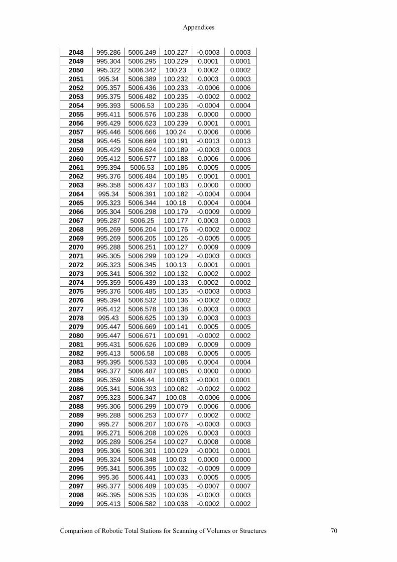
Appendices
2048 995.286 5006.249 100.227 -0.0003 0.0003 2049 995.304 5006.295 100.229 0.0001 0.0001 2050 995.322 5006.342 100.23 0.0002 0.0002 2051 995.34 5006.389 100.232 0.0003 0.0003 2052 995.357 5006.436 100.233 -0.0006 0.0006 2053 995.375 5006.482 100.235 -0.0002 0.0002 2054 995.393 5006.53 100.236 -0.0004 0.0004 2055 995.411 5006.576 100.238 0.0000 0.0000 2056 995.429 5006.623 100.239 0.0001 0.0001 2057 995.446 5006.666 100.24 0.0006 0.0006 2058 995.445 5006.669 100.191 -0.0013 0.0013 2059 995.429 5006.624 100.189 -0.0003 0.0003 2060 995.412 5006.577 100.188 0.0006 0.0006 2061 995.394 5006.53 100.186 0.0005 0.0005 2062 995.376 5006.484 100.185 0.0001 0.0001 2063 995.358 5006.437 100.183 0.0000 0.0000 2064 995.34 5006.391 100.182 -0.0004 0.0004 2065 995.323 5006.344 100.18 0.0004 0.0004 2066 995.304 5006.298 100.179 -0.0009 0.0009 2067 995.287 5006.25 100.177 0.0003 0.0003 2068 995.269 5006.204 100.176 -0.0002 0.0002 2069 995.269 5006.205 100.126 -0.0005 0.0005 2070 995.288 5006.251 100.127 0.0009 0.0009 2071 995.305 5006.299 100.129 -0.0003 0.0003 2072 995.323 5006.345 100.13 0.0001 0.0001 2073 995.341 5006.392 100.132 0.0002 0.0002 2074 995.359 5006.439 100.133 0.0002 0.0002 2075 995.376 5006.485 100.135 -0.0003 0.0003 2076 995.394 5006.532 100.136 -0.0002 0.0002 2077 995.412 5006.578 100.138 0.0003 0.0003 2078 995.43 5006.625 100.139 0.0003 0.0003 2079 995.447 5006.669 100.141 0.0005 0.0005 2080 995.447 5006.671 100.091 -0.0002 0.0002 2081 995.431 5006.626 100.089 0.0009 0.0009 2082 995.413 5006.58 100.088 0.0005 0.0005 2083 995.395 5006.533 100.086 0.0004 0.0004 2084 995.377 5006.487 100.085 0.0000 0.0000 2085 995.359 5006.44 100.083 -0.0001 0.0001 2086 995.341 5006.393 100.082 -0.0002 0.0002 2087 995.323 5006.347 100.08 -0.0006 0.0006 2088 995.306 5006.299 100.079 0.0006 0.0006 2089 995.288 5006.253 100.077 0.0002 0.0002 2090 995.27 5006.207 100.076 -0.0003 0.0003 2091 995.271 5006.208 100.026 0.0003 0.0003 2092 995.289 5006.254 100.027 0.0008 0.0008 2093 995.306 5006.301 100.029 -0.0001 0.0001 2094 995.324 5006.348 100.03 0.0000 0.0000 2095 995.341 5006.395 100.032 -0.0009 0.0009 2096 995.36 5006.441 100.033 0.0005 0.0005 2097 995.377 5006.489 100.035 -0.0007 0.0007 2098 995.395 5006.535 100.036 -0.0003 0.0003 2099 995.413 5006.582 100.038 -0.0002 0.0002
Comparison of Robotic Total Stations for Scanning of Volumes or Structures 70

Appendices
2100 995.431 5006.628 100.039 0.0002 0.0002 2101 995.447 5006.672 100.041 -0.0005 0.0005 2102 995.448 5006.673 99.991 0.0001 0.0001 2103 995.431 5006.63 99.989 -0.0005 0.0005 2104 995.414 5006.583 99.988 0.0004 0.0004 2105 995.396 5006.537 99.986 0.0000 0.0000 2106 995.378 5006.49 99.985 -0.0001 0.0001 2107 995.36 5006.443 99.983 -0.0002 0.0002 2108 995.342 5006.396 99.982 -0.0003 0.0003 2109 995.325 5006.349 99.98 0.0006 0.0006 2110 995.306 5006.303 99.979 -0.0008 0.0008 2111 995.289 5006.256 99.977 0.0001 0.0001 2112 995.272 5006.209 99.976 0.0009 0.0009 2113 995.272 5006.21 99.927 0.0006 0.0006 2114 995.289 5006.257 99.928 -0.0003 0.0003 2115 995.307 5006.304 99.93 -0.0002 0.0002 2116 995.325 5006.351 99.931 -0.0001 0.0001 2117 995.342 5006.398 99.933 -0.0010 0.0010 2118 995.361 5006.444 99.934 0.0004 0.0004 2119 995.378 5006.491 99.936 -0.0005 0.0005 2120 995.396 5006.538 99.937 -0.0004 0.0004 2121 995.414 5006.585 99.939 -0.0003 0.0003 2122 995.432 5006.631 99.94 0.0001 0.0001 2123 995.449 5006.675 99.941 0.0003 0.0003
Comparison of Robotic Total Stations for Scanning of Volumes or Structures 71
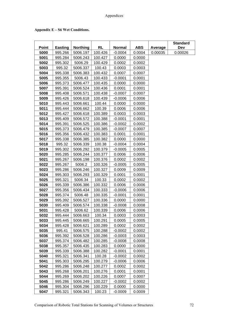
Appendices
Appendix E – S6 Wet Conditions.
Point Easting Northing RL Normal ABS Average Standard
Dev 5000 995.266 5006.197 100.426 -0.0004 0.0004 0.00035 0.00026 5001 995.284 5006.243 100.427 0.0000 0.0000 5002 995.302 5006.29 100.429 0.0002 0.0002 5003 995.32 5006.337 100.43 0.0003 0.0003 5004 995.338 5006.383 100.432 0.0007 0.0007 5005 995.355 5006.43 100.433 -0.0001 0.0001 5006 995.373 5006.477 100.435 0.0000 0.0000 5007 995.391 5006.524 100.436 0.0001 0.0001 5008 995.408 5006.571 100.438 -0.0007 0.0007 5009 995.426 5006.618 100.439 -0.0006 0.0006 5010 995.443 5006.661 100.44 0.0000 0.0000 5011 995.444 5006.662 100.39 0.0006 0.0006 5012 995.427 5006.618 100.389 0.0003 0.0003 5013 995.409 5006.572 100.388 -0.0001 0.0001 5014 995.391 5006.525 100.386 -0.0002 0.0002 5015 995.373 5006.479 100.385 -0.0007 0.0007 5016 995.356 5006.432 100.383 0.0001 0.0001 5017 995.338 5006.385 100.382 0.0000 0.0000 5018 995.32 5006.339 100.38 -0.0004 0.0004 5019 995.302 5006.292 100.379 -0.0005 0.0005 5020 995.285 5006.244 100.377 0.0006 0.0006 5021 995.267 5006.198 100.376 0.0002 0.0002 5022 995.267 5006.2 100.326 -0.0005 0.0005 5023 995.286 5006.246 100.327 0.0009 0.0009 5024 995.303 5006.293 100.329 0.0001 0.0001 5025 995.321 5006.34 100.33 0.0002 0.0002 5026 995.339 5006.386 100.332 0.0006 0.0006 5027 995.356 5006.434 100.333 -0.0006 0.0006 5028 995.374 5006.48 100.335 -0.0001 0.0001 5029 995.392 5006.527 100.336 0.0000 0.0000 5030 995.409 5006.574 100.338 -0.0008 0.0008 5031 995.428 5006.62 100.339 0.0006 0.0006 5032 995.444 5006.663 100.34 0.0003 0.0003 5033 995.445 5006.665 100.291 0.0005 0.0005 5034 995.428 5006.621 100.289 0.0002 0.0002 5035 995.41 5006.575 100.288 -0.0002 0.0002 5036 995.392 5006.528 100.286 -0.0003 0.0003 5037 995.374 5006.482 100.285 -0.0008 0.0008 5038 995.357 5006.435 100.283 0.0000 0.0000 5039 995.339 5006.388 100.282 -0.0001 0.0001 5040 995.321 5006.341 100.28 -0.0002 0.0002 5041 995.303 5006.295 100.279 -0.0006 0.0006 5042 995.286 5006.248 100.277 0.0002 0.0002 5043 995.268 5006.201 100.276 0.0001 0.0001 5044 995.269 5006.202 100.226 0.0007 0.0007 5045 995.286 5006.249 100.227 -0.0002 0.0002 5046 995.304 5006.296 100.229 0.0000 0.0000 5047 995.321 5006.343 100.23 -0.0009 0.0009
Comparison of Robotic Total Stations for Scanning of Volumes or Structures 72

Appendices
5048 995.339 5006.389 100.232 -0.0004 0.0004 5049 995.358 5006.436 100.233 0.0006 0.0006 5050 995.375 5006.483 100.235 -0.0002 0.0002 5051 995.393 5006.529 100.236 0.0003 0.0003 5052 995.411 5006.576 100.238 0.0004 0.0004 5053 995.429 5006.622 100.239 0.0008 0.0008 5054 995.445 5006.667 100.241 -0.0002 0.0002 5055 995.446 5006.668 100.191 0.0004 0.0004 5056 995.429 5006.624 100.189 0.0001 0.0001 5057 995.412 5006.577 100.188 0.0010 0.0010 5058 995.393 5006.531 100.186 -0.0004 0.0004 5059 995.376 5006.484 100.185 0.0004 0.0004 5060 995.358 5006.437 100.183 0.0003 0.0003 5061 995.34 5006.391 100.182 -0.0002 0.0002 5062 995.322 5006.344 100.18 -0.0003 0.0003 5063 995.305 5006.297 100.179 0.0005 0.0005 5064 995.287 5006.251 100.177 0.0001 0.0001 5065 995.269 5006.204 100.176 0.0000 0.0000 5066 995.269 5006.206 100.126 -0.0007 0.0007 5067 995.287 5006.252 100.127 -0.0003 0.0003 5068 995.306 5006.298 100.129 0.0011 0.0011 5069 995.323 5006.345 100.13 0.0003 0.0003 5070 995.34 5006.392 100.132 -0.0005 0.0005 5071 995.359 5006.439 100.133 0.0005 0.0005 5072 995.376 5006.485 100.135 0.0001 0.0001 5073 995.394 5006.532 100.136 0.0002 0.0002 5074 995.412 5006.579 100.138 0.0003 0.0003 5075 995.429 5006.626 100.139 -0.0005 0.0005 5076 995.446 5006.669 100.141 0.0000 0.0000 5077 995.447 5006.671 100.091 0.0003 0.0003 5078 995.43 5006.627 100.089 0.0000 0.0000 5079 995.412 5006.581 100.088 -0.0004 0.0004 5080 995.394 5006.534 100.086 -0.0005 0.0005 5081 995.376 5006.487 100.085 -0.0006 0.0006 5082 995.359 5006.44 100.083 0.0002 0.0002 5083 995.341 5006.393 100.082 0.0001 0.0001 5084 995.323 5006.347 100.08 -0.0004 0.0004 5085 995.306 5006.3 100.079 0.0004 0.0004 5086 995.288 5006.254 100.077 0.0000 0.0000 5087 995.27 5006.207 100.076 -0.0001 0.0001 5088 995.271 5006.208 100.026 0.0005 0.0005 5089 995.288 5006.255 100.027 -0.0004 0.0004 5090 995.306 5006.302 100.029 -0.0003 0.0003 5091 995.324 5006.349 100.03 -0.0001 0.0001 5092 995.341 5006.395 100.032 -0.0006 0.0006 5093 995.359 5006.442 100.033 -0.0005 0.0005 5094 995.377 5006.489 100.035 -0.0004 0.0004 5095 995.395 5006.535 100.036 0.0001 0.0001 5096 995.413 5006.582 100.038 0.0002 0.0002 5097 995.43 5006.629 100.039 -0.0006 0.0006 5098 995.447 5006.673 100.041 -0.0004 0.0004 5099 995.448 5006.673 99.991 0.0005 0.0005
Comparison of Robotic Total Stations for Scanning of Volumes or Structures 73
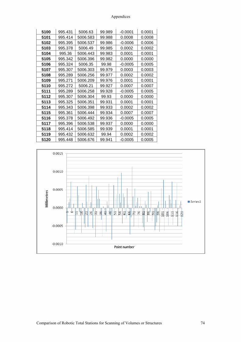
Appendices
5100 995.431 5006.63 99.989 -0.0001 0.0001 5101 995.414 5006.583 99.988 0.0008 0.0008 5102 995.395 5006.537 99.986 -0.0006 0.0006 5103 995.378 5006.49 99.985 0.0002 0.0002 5104 995.36 5006.443 99.983 0.0001 0.0001 5105 995.342 5006.396 99.982 0.0000 0.0000 5106 995.324 5006.35 99.98 -0.0005 0.0005 5107 995.307 5006.303 99.979 0.0003 0.0003 5108 995.289 5006.256 99.977 0.0002 0.0002 5109 995.271 5006.209 99.976 0.0001 0.0001 5110 995.272 5006.21 99.927 0.0007 0.0007 5111 995.289 5006.258 99.928 -0.0005 0.0005 5112 995.307 5006.304 99.93 0.0000 0.0000 5113 995.325 5006.351 99.931 0.0001 0.0001 5114 995.343 5006.398 99.933 0.0002 0.0002 5115 995.361 5006.444 99.934 0.0007 0.0007 5116 995.378 5006.492 99.936 -0.0005 0.0005 5117 995.396 5006.538 99.937 0.0000 0.0000 5118 995.414 5006.585 99.939 0.0001 0.0001 5119 995.432 5006.632 99.94 0.0002 0.0002 5120 995.448 5006.676 99.941 -0.0005 0.0005
Comparison of Robotic Total Stations for Scanning of Volumes or Structures 74

Appendices
Appendix F – Leica Dry Conditions.
Point Easting Northing RL Normal ABS Average Standard
Dev 2000 995.265 5006.198 101.94 0.0013 0.0013 0.00041 0.00027 2001 995.282 5006.246 101.94 0.0002 0.0002 2002 995.3 5006.293 101.94 0.0003 0.0003 2003 995.317 5006.34 101.94 -0.0005 0.0005 2004 995.335 5006.386 101.94 0.0000 0.0000 2005 995.353 5006.433 101.94 0.0002 0.0002 2006 995.37 5006.481 101.94 -0.0010 0.0010 2007 995.388 5006.527 101.94 -0.0005 0.0005 2008 995.406 5006.573 101.94 0.0001 0.0001 2009 995.424 5006.62 101.94 0.0002 0.0002 2010 995.424 5006.621 101.89 -0.0001 0.0001 2011 995.406 5006.573 101.89 0.0001 0.0001 2012 995.389 5006.526 101.89 0.0009 0.0009 2013 995.37 5006.48 101.89 -0.0006 0.0006 2014 995.353 5006.433 101.89 0.0002 0.0002 2015 995.335 5006.387 101.89 -0.0003 0.0003 2016 995.317 5006.34 101.89 -0.0004 0.0004 2017 995.3 5006.292 101.89 0.0007 0.0007 2018 995.282 5006.246 101.89 0.0002 0.0002 2019 995.264 5006.2 101.89 -0.0003 0.0003 2020 995.264 5006.199 101.84 0.0001 0.0001 2021 995.282 5006.245 101.84 0.0006 0.0006 2022 995.3 5006.293 101.84 0.0004 0.0004 2023 995.317 5006.339 101.84 0.0000 0.0000 2024 995.335 5006.386 101.84 0.0001 0.0001 2025 995.353 5006.432 101.84 0.0006 0.0006 2026 995.371 5006.479 101.84 0.0008 0.0008 2027 995.388 5006.526 101.84 0.0000 0.0000 2028 995.406 5006.573 101.84 0.0001 0.0001 2029 995.423 5006.621 101.84 -0.0010 0.0010 2030 995.424 5006.62 101.79 0.0003 0.0003 2031 995.406 5006.573 101.79 0.0001 0.0001 2032 995.388 5006.526 101.79 0.0000 0.0000 2033 995.371 5006.479 101.79 0.0008 0.0008 2034 995.353 5006.433 101.79 0.0003 0.0003 2035 995.335 5006.387 101.79 -0.0002 0.0002 2036 995.317 5006.34 101.79 -0.0004 0.0004 2037 995.3 5006.292 101.79 0.0008 0.0008 2038 995.282 5006.246 101.79 0.0003 0.0003 2039 995.263 5006.2 101.79 -0.0012 0.0012 2040 995.264 5006.199 101.74 0.0002 0.0002 2041 995.281 5006.247 101.74 -0.0010 0.0010 2042 995.299 5006.293 101.74 -0.0005 0.0005 2043 995.317 5006.34 101.74 -0.0003 0.0003 2044 995.335 5006.386 101.74 0.0002 0.0002 2045 995.353 5006.433 101.74 0.0003 0.0003 2046 995.37 5006.48 101.74 -0.0005 0.0005 2047 995.388 5006.527 101.74 -0.0003 0.0003
Comparison of Robotic Total Stations for Scanning of Volumes or Structures 75
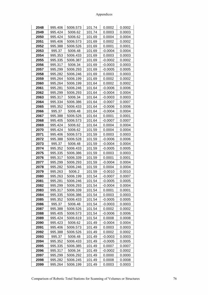
Appendices
2048 995.406 5006.573 101.74 0.0002 0.0002 2049 995.424 5006.62 101.74 0.0003 0.0003 2050 995.424 5006.62 101.69 0.0004 0.0004 2051 995.406 5006.573 101.69 0.0002 0.0002 2052 995.388 5006.526 101.69 0.0001 0.0001 2053 995.37 5006.48 101.69 -0.0004 0.0004 2054 995.353 5006.433 101.69 0.0003 0.0003 2055 995.335 5006.387 101.69 -0.0002 0.0002 2056 995.317 5006.34 101.69 -0.0003 0.0003 2057 995.299 5006.293 101.69 -0.0005 0.0005 2058 995.282 5006.246 101.69 0.0003 0.0003 2059 995.264 5006.199 101.69 0.0002 0.0002 2060 995.264 5006.199 101.64 0.0002 0.0002 2061 995.281 5006.246 101.64 -0.0006 0.0006 2062 995.299 5006.293 101.64 -0.0004 0.0004 2063 995.317 5006.34 101.64 -0.0003 0.0003 2064 995.334 5006.386 101.64 -0.0007 0.0007 2065 995.352 5006.433 101.64 -0.0006 0.0006 2066 995.37 5006.48 101.64 -0.0004 0.0004 2067 995.388 5006.526 101.64 0.0001 0.0001 2068 995.405 5006.573 101.64 -0.0007 0.0007 2069 995.424 5006.62 101.64 0.0004 0.0004 2070 995.424 5006.62 101.59 0.0004 0.0004 2071 995.406 5006.573 101.59 0.0003 0.0003 2072 995.388 5006.528 101.59 -0.0006 0.0006 2073 995.37 5006.48 101.59 -0.0004 0.0004 2074 995.352 5006.433 101.59 -0.0005 0.0005 2075 995.335 5006.386 101.59 0.0003 0.0003 2076 995.317 5006.339 101.59 0.0001 0.0001 2077 995.299 5006.293 101.59 -0.0004 0.0004 2078 995.282 5006.246 101.59 0.0004 0.0004 2079 995.263 5006.2 101.59 -0.0010 0.0010 2080 995.263 5006.199 101.54 -0.0007 0.0007 2081 995.281 5006.246 101.54 -0.0005 0.0005 2082 995.299 5006.293 101.54 -0.0004 0.0004 2083 995.317 5006.339 101.54 0.0001 0.0001 2084 995.335 5006.386 101.54 0.0003 0.0003 2085 995.352 5006.433 101.54 -0.0005 0.0005 2086 995.37 5006.48 101.54 -0.0003 0.0003 2087 995.388 5006.526 101.54 0.0002 0.0002 2088 995.405 5006.573 101.54 -0.0006 0.0006 2089 995.424 5006.619 101.54 0.0008 0.0008 2090 995.423 5006.62 101.49 -0.0004 0.0004 2091 995.406 5006.573 101.49 0.0003 0.0003 2092 995.388 5006.526 101.49 0.0002 0.0002 2093 995.37 5006.48 101.49 -0.0003 0.0003 2094 995.352 5006.433 101.49 -0.0005 0.0005 2095 995.335 5006.385 101.49 0.0007 0.0007 2096 995.317 5006.34 101.49 -0.0002 0.0002 2097 995.299 5006.292 101.49 0.0000 0.0000 2098 995.282 5006.245 101.49 0.0008 0.0008 2099 995.264 5006.199 101.49 0.0003 0.0003
Comparison of Robotic Total Stations for Scanning of Volumes or Structures 76

Appendices
2100 995.264 5006.198 101.44 0.0007 0.0007 2101 995.282 5006.246 101.44 0.0005 0.0005 2102 995.299 5006.293 101.44 -0.0003 0.0003 2103 995.317 5006.339 101.44 0.0002 0.0002 2104 995.335 5006.385 101.44 0.0007 0.0007 2105 995.353 5006.432 101.44 0.0009 0.0009 2106 995.371 5006.479 101.44 0.0010 0.0010 2107 995.388 5006.526 101.44 0.0002 0.0002 2108 995.405 5006.573 101.44 -0.0006 0.0006 2109 995.423 5006.62 101.44 -0.0004 0.0004
Comparison of Robotic Total Stations for Scanning of Volumes or Structures 77

Appendices
Appendix G – Leica Wet Conditions.
Point Easting Northing RL Normal ABS Average Standard
Dev 4000 995.264 5006.199 101.94 0.0005 0.0005 0.00035 0.00025 4001 995.282 5006.247 101.94 0.0002 0.0002 4002 995.299 5006.294 101.94 -0.0006 0.0006 4003 995.317 5006.34 101.94 -0.0001 0.0001 4004 995.335 5006.386 101.94 0.0003 0.0003 4005 995.353 5006.433 101.94 0.0004 0.0004 4006 995.37 5006.481 101.94 -0.0008 0.0008 4007 995.388 5006.527 101.94 -0.0003 0.0003 4008 995.406 5006.573 101.94 0.0001 0.0001 4009 995.424 5006.62 101.94 0.0002 0.0002 4010 995.424 5006.621 101.89 -0.0001 0.0001 4011 995.406 5006.574 101.89 -0.0002 0.0002 4012 995.388 5006.527 101.89 -0.0003 0.0003 4013 995.37 5006.481 101.89 -0.0008 0.0008 4014 995.353 5006.433 101.89 0.0004 0.0004 4015 995.335 5006.387 101.89 0.0000 0.0000 4016 995.317 5006.34 101.89 -0.0001 0.0001 4017 995.299 5006.293 101.89 -0.0002 0.0002 4018 995.282 5006.246 101.89 0.0006 0.0006 4019 995.264 5006.2 101.89 0.0002 0.0002 4020 995.264 5006.199 101.84 0.0006 0.0006 4021 995.281 5006.246 101.84 -0.0003 0.0003 4022 995.299 5006.293 101.84 -0.0002 0.0002 4023 995.317 5006.339 101.84 0.0003 0.0003 4024 995.335 5006.387 101.84 0.0000 0.0000 4025 995.353 5006.433 101.84 0.0005 0.0005 4026 995.37 5006.48 101.84 -0.0004 0.0004 4027 995.388 5006.527 101.84 -0.0003 0.0003 4028 995.406 5006.574 101.84 -0.0002 0.0002 4029 995.424 5006.62 101.84 0.0003 0.0003 4030 995.424 5006.62 101.79 0.0003 0.0003 4031 995.406 5006.573 101.79 0.0002 0.0002 4032 995.388 5006.527 101.79 -0.0002 0.0002 4033 995.371 5006.479 101.79 0.0009 0.0009 4034 995.353 5006.433 101.79 0.0005 0.0005 4035 995.335 5006.387 101.79 0.0000 0.0000 4036 995.318 5006.339 101.79 0.0012 0.0012 4037 995.299 5006.293 101.79 -0.0002 0.0002 4038 995.281 5006.247 101.79 -0.0006 0.0006 4039 995.264 5006.199 101.79 0.0006 0.0006 4040 995.264 5006.2 101.74 0.0003 0.0003 4041 995.281 5006.247 101.74 -0.0006 0.0006 4042 995.299 5006.294 101.74 -0.0005 0.0005 4043 995.317 5006.341 101.74 -0.0004 0.0004 4044 995.335 5006.386 101.74 0.0004 0.0004 4045 995.352 5006.434 101.74 -0.0008 0.0008 4046 995.37 5006.48 101.74 -0.0003 0.0003 4047 995.388 5006.527 101.74 -0.0002 0.0002
Comparison of Robotic Total Stations for Scanning of Volumes or Structures 78
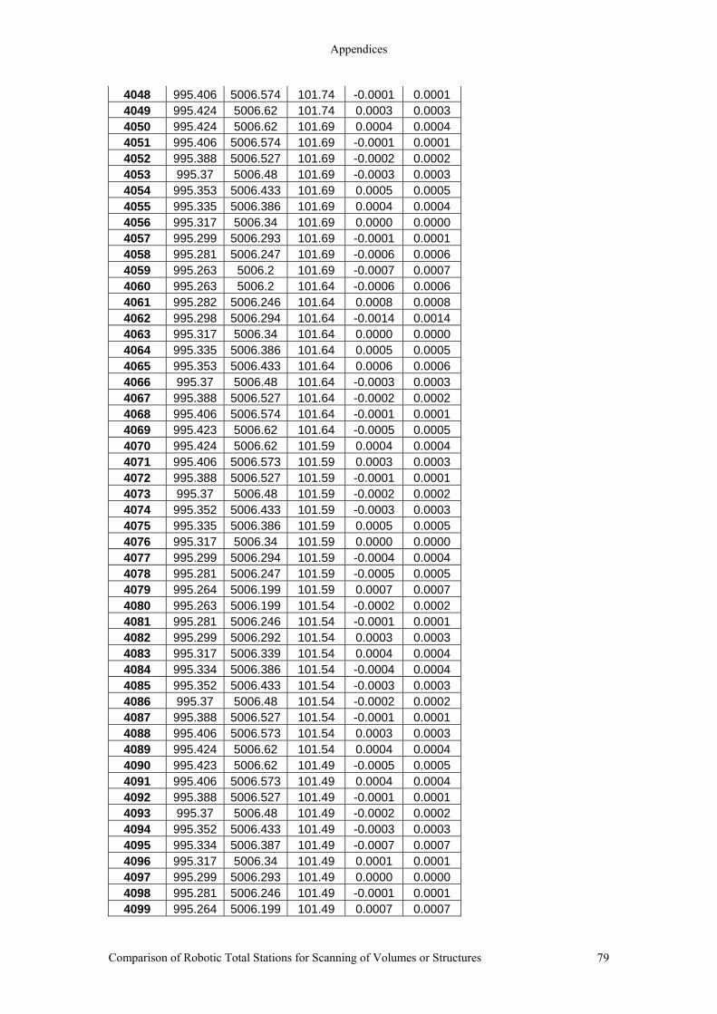
Appendices
4048 995.406 5006.574 101.74 -0.0001 0.0001 4049 995.424 5006.62 101.74 0.0003 0.0003 4050 995.424 5006.62 101.69 0.0004 0.0004 4051 995.406 5006.574 101.69 -0.0001 0.0001 4052 995.388 5006.527 101.69 -0.0002 0.0002 4053 995.37 5006.48 101.69 -0.0003 0.0003 4054 995.353 5006.433 101.69 0.0005 0.0005 4055 995.335 5006.386 101.69 0.0004 0.0004 4056 995.317 5006.34 101.69 0.0000 0.0000 4057 995.299 5006.293 101.69 -0.0001 0.0001 4058 995.281 5006.247 101.69 -0.0006 0.0006 4059 995.263 5006.2 101.69 -0.0007 0.0007 4060 995.263 5006.2 101.64 -0.0006 0.0006 4061 995.282 5006.246 101.64 0.0008 0.0008 4062 995.298 5006.294 101.64 -0.0014 0.0014 4063 995.317 5006.34 101.64 0.0000 0.0000 4064 995.335 5006.386 101.64 0.0005 0.0005 4065 995.353 5006.433 101.64 0.0006 0.0006 4066 995.37 5006.48 101.64 -0.0003 0.0003 4067 995.388 5006.527 101.64 -0.0002 0.0002 4068 995.406 5006.574 101.64 -0.0001 0.0001 4069 995.423 5006.62 101.64 -0.0005 0.0005 4070 995.424 5006.62 101.59 0.0004 0.0004 4071 995.406 5006.573 101.59 0.0003 0.0003 4072 995.388 5006.527 101.59 -0.0001 0.0001 4073 995.37 5006.48 101.59 -0.0002 0.0002 4074 995.352 5006.433 101.59 -0.0003 0.0003 4075 995.335 5006.386 101.59 0.0005 0.0005 4076 995.317 5006.34 101.59 0.0000 0.0000 4077 995.299 5006.294 101.59 -0.0004 0.0004 4078 995.281 5006.247 101.59 -0.0005 0.0005 4079 995.264 5006.199 101.59 0.0007 0.0007 4080 995.263 5006.199 101.54 -0.0002 0.0002 4081 995.281 5006.246 101.54 -0.0001 0.0001 4082 995.299 5006.292 101.54 0.0003 0.0003 4083 995.317 5006.339 101.54 0.0004 0.0004 4084 995.334 5006.386 101.54 -0.0004 0.0004 4085 995.352 5006.433 101.54 -0.0003 0.0003 4086 995.37 5006.48 101.54 -0.0002 0.0002 4087 995.388 5006.527 101.54 -0.0001 0.0001 4088 995.406 5006.573 101.54 0.0003 0.0003 4089 995.424 5006.62 101.54 0.0004 0.0004 4090 995.423 5006.62 101.49 -0.0005 0.0005 4091 995.406 5006.573 101.49 0.0004 0.0004 4092 995.388 5006.527 101.49 -0.0001 0.0001 4093 995.37 5006.48 101.49 -0.0002 0.0002 4094 995.352 5006.433 101.49 -0.0003 0.0003 4095 995.334 5006.387 101.49 -0.0007 0.0007 4096 995.317 5006.34 101.49 0.0001 0.0001 4097 995.299 5006.293 101.49 0.0000 0.0000 4098 995.281 5006.246 101.49 -0.0001 0.0001 4099 995.264 5006.199 101.49 0.0007 0.0007
Comparison of Robotic Total Stations for Scanning of Volumes or Structures 79

Appendices
4100 995.263 5006.199 101.44 -0.0002 0.0002 4101 995.281 5006.246 101.44 -0.0001 0.0001 4102 995.299 5006.293 101.44 0.0000 0.0000 4103 995.317 5006.339 101.44 0.0005 0.0005 4104 995.335 5006.386 101.44 0.0006 0.0006 4105 995.352 5006.432 101.44 0.0001 0.0001 4106 995.37 5006.48 101.44 -0.0002 0.0002 4107 995.388 5006.526 101.44 0.0003 0.0003 4108 995.406 5006.573 101.44 0.0004 0.0004 4109 995.423 5006.62 101.44 -0.0004 0.0004
Comparison of Robotic Total Stations for Scanning of Volumes or Structures 80

Appendices
Appendix H – Chainage and Offset Report, Terramodel
SMK Consultants Pty. Ltd. PO BOX 422 GOONDIWINDI,4390 Tel (07)4671 2445 ; Fax (07)4671 2561 Tuesday, October 20, 2009 5:47:01 PM PROJECT: roject Part 2\Jeff Dissertation\Encroachment\Trimble S6\Trimble S6.pro -------------------------------------------------------------------------------- ALIGNMENT REPORT Alignment Name: Free Pts Point Number Description Chainage Easting Northing Elevation Offset -------------------------------------------------------------------------------- 1000 WAL 0.003 996.714 1006.897 102.588 WAL 0.003 1001 WAL 0.005 996.714 1006.894 101.385 WAL 0.002 1002 WAL 2.646 996.714 1006.892 100.209 WAL 2.640 1003 WAL 2.649 996.669 1004.252 102.590 WAL 0.003 1004 WAL 2.658 996.670 1004.249 101.389 WAL 0.009 1005 WAL 3.083 996.679 1004.250 100.200 WAL 0.424 1006 WAL 3.088 996.431 1003.906 100.191 WAL 0.006 1007 WAL 3.093 996.425 1003.906 101.391 WAL 0.004 1008 WAL 7.681 996.422 1003.909 102.591 WAL 4.588 1009 WAL 7.684 991.834 1003.970 102.591 WAL 0.003 1010 WAL 7.686 991.832 1003.972 101.384 WAL 0.003 1011 WAL 8.009 991.829 1003.973 100.190 WAL 0.322 1012 NS 16.916 992.071 1003.760 100.101 NS 8.908
Comparison of Robotic Total Stations for Scanning of Volumes or Structures 81
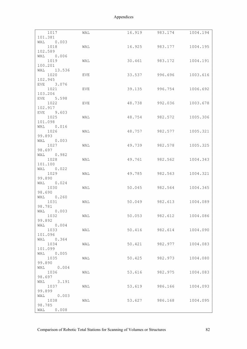
Appendices
1017 WAL 16.919 983.174 1004.194 101.381 WAL 0.003 1018 WAL 16.925 983.177 1004.195 102.589 WAL 0.006 1019 WAL 30.461 983.172 1004.191 100.201 WAL 13.536 1020 EVE 33.537 996.696 1003.616 102.945 EVE 3.076 1021 EVE 39.135 996.754 1006.692 103.206 EVE 5.598 1022 EVE 48.738 992.036 1003.678 102.917 EVE 9.603 1025 WAL 48.754 982.572 1005.306 101.098 WAL 0.016 1026 WAL 48.757 982.577 1005.321 99.893 WAL 0.003 1027 WAL 49.739 982.578 1005.325 98.697 WAL 0.982 1028 WAL 49.761 982.562 1004.343 101.100 WAL 0.022 1029 WAL 49.785 982.563 1004.321 99.890 WAL 0.024 1030 WAL 50.045 982.564 1004.345 98.690 WAL 0.260 1031 WAL 50.049 982.613 1004.089 98.781 WAL 0.003 1032 WAL 50.053 982.612 1004.086 99.892 WAL 0.004 1033 WAL 50.416 982.614 1004.090 101.096 WAL 0.364 1034 WAL 50.421 982.977 1004.083 101.099 WAL 0.005 1035 WAL 50.425 982.973 1004.080 99.890 WAL 0.004 1036 WAL 53.616 982.975 1004.083 98.697 WAL 3.191 1037 WAL 53.619 986.166 1004.093 99.899 WAL 0.003 1038 WAL 53.627 986.168 1004.095 98.785 WAL 0.008
Comparison of Robotic Total Stations for Scanning of Volumes or Structures 82
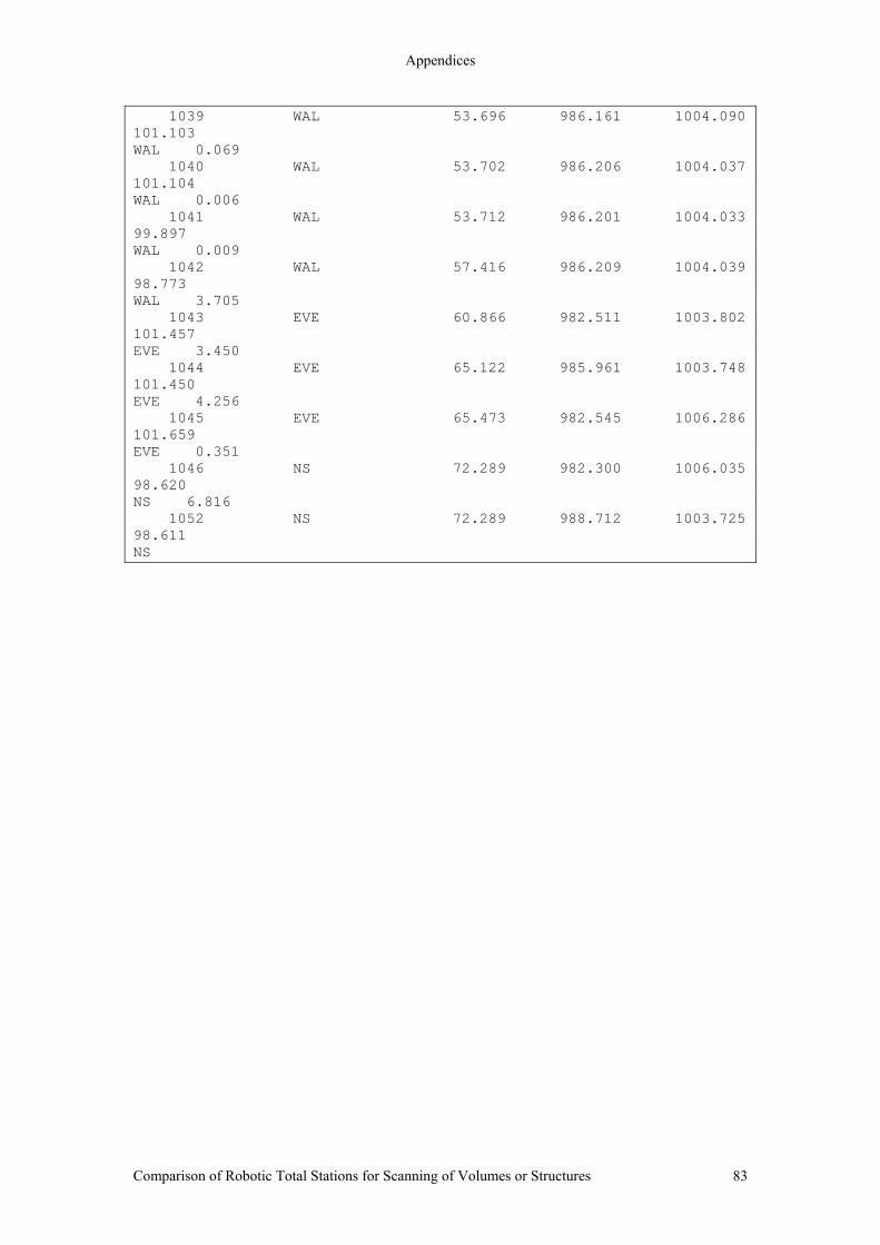
Appendices
1039 WAL 53.696 986.161 1004.090 101.103 WAL 0.069 1040 WAL 53.702 986.206 1004.037 101.104 WAL 0.006 1041 WAL 53.712 986.201 1004.033 99.897 WAL 0.009 1042 WAL 57.416 986.209 1004.039 98.773 WAL 3.705 1043 EVE 60.866 982.511 1003.802 101.457 EVE 3.450 1044 EVE 65.122 985.961 1003.748 101.450 EVE 4.256 1045 EVE 65.473 982.545 1006.286 101.659 EVE 0.351 1046 NS 72.289 982.300 1006.035 98.620 NS 6.816 1052 NS 72.289 988.712 1003.725 98.611 NS
Comparison of Robotic Total Stations for Scanning of Volumes or Structures 83
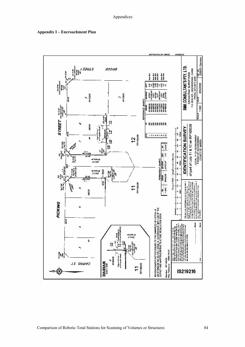
Appendices
Comparison of Robotic Total Stations for Scanning of Volumes or Structures 84
Appendix I – Encroachment Plan