Master Thesis Naval Architecture 2002-2003 January 20th, 2004

COMPARISON OF ÅSGARD B PLATFORM’S FIELD MEASUREMENT AND TIME DOMAIN NUMERICAL SIMULATIONS OTUNOLA, ABIODUN ADEBAYO

Water Environment Transport CHALMERS UNIVERSITY OF TECHNOLOGY S-412 96, Göteborg, Sweden

Master’s Thesis 2003:24

1

iii

ABSTRACT Moored floating platforms are used for drilling and exploration activates and they require high degree of precise positioning to perform optimally with associated facilities. They are subjected to combined environmental loads of waves, wind and current while in service, which affects their stability in addition to positioning. Dynamic analysis of a floating moored platform is therefore carried out to determine its response to environmental loads. This analysis could be done in the time domain or the frequency domain. A floating platform is associated with lots of non-linearities, which are linearised in the frequency domain simulations. In the time domain analysis however, the non-linearities are modelled with the intention of making more accurate analysis but this makes the computation complex and require a great deal of computer time. GVA Consultants have developed software, CASH (Coupled Analysis Software for Hydrodynamics) for time domain analysis of a moored floating platform. The program performs dynamic analysis in a combined state (low-frequency and wave –frequency) in the six degrees of freedom. The program had earlier been verified against other software and a good agreement has also been obtained between CASH and model test. The objective of the thesis work therefore is to compare CASH simulation with measured field data STATOIL has measured the environmental loads, motion responses and line tensions of Åsgard B semi-submersible platform in the North Sea and data are to be used for CASH simulation and results compared afterwards . The model test performed on Åsgard B was used to calibrate wind, current and wave drift force coefficients which form part of the input to CASH for the field environmental load analysis. Three different sea states (in increasing order) were selected from the measured field data to perform CASH analysis. CASH numerical simulations agreed with the model test results and measured field data in terms of mean offsets and mean line tensions. The disparity in standard deviation is suggested for further investigation.

iv

ACKNOWLEDGEMENT

It is not if him that willeth or him that runneth, but of the Lord that showed mercy….I thank God almighty for His grace, protection, provision and mercy upon me while my study lasted in Sweden, if not Him, I can not do anything, but with Him , I can do all things, thank you Lord! I also than my parents Mr and Mrs Joseph Alabi Odofin who put me on the noble path of education at a tender age of five, I appreciate you! I thank my program co-ordinator, Prof. Anders Ulvarson, for his support and guidance throughout my study, and my thesis supervisor, Prof. Lars Bergdahl for his invaluable contributions to the thesis work. The assistance of GVA Consultants is highly appreciated. I thank Mr Pontus Clason, Dr Yungang Liu and Mr Daniel Aneljung, you are all wonderful!. My appreciation also goes to my Pastor, Tutu Olutayo and his family for their prayer and counselling, may the Lord continue to increase you in Jesus name, Amen and also to the wonderful family of Deacon Isacc Ileso, I say a big thank you, To all my friends, I say thank you for making my stay eventful, Borther Kazeen Olanrewaju, Sina Morenighade, Osarobo, Fred, Bolaji, Sadiq, Emeka, Lateef, Dr. Felix, Kenneth, Samuel, Tony, and others too numerous to mention, thank you all. Finally, I wish to express my deep and heartfelt gratitude to my inestimable jewel, Zainab Nene Anike Otunola. I appreciate your prayers, sacrifice, and perseverance during my absence, you are living proof of unconditional love and support, I love you dear!

v

ABSTRACT……………………………………………………………………………………….iii ACKNOWLEDGEMENT………………………………………………………………………..iv

LIST OF FIGURES………………………………………………………………………………vii

LIST OF TABLES………………………………………………………………………………..viii

1 INTRODUCTION.................................................................................................................... 1 1.1 BACKGROUND......................................................................................................................... 1 1.2 OBJECTIVE AND SCOPE OF WORK ............................................................................................ 2 1.3 APPROACH .............................................................................................................................. 3

2 OFFSHORE STRUCTURES.................................................................................................. 4 2.1 SEMI-SUBMERSIBLE ................................................................................................................ 4 2.2 TENSION LEG PLATFORM (TLP) ............................................................................................. 4 2.3 GUYED TOWER ....................................................................................................................... 4 2.4 JACK-UP DRILLING RIG .......................................................................................................... 5 2.5 GRAVITY STRUCTURE............................................................................................................. 5 2.6 FIXED JACKETED STRUCTURE................................................................................................. 5 2.7 ARTICULATED TOWER AND SINGLE ANCHOR LEG MOORED SYSTEMS ................................... 6 2.8 FLOATING PLATFORM VERSUS FIXED PLATFORM .................................................................... 6 2.9 SPAR PLATFORM ..................................................................................................................... 6

3 ENVIRONMENTAL LOADS AND FORCES ON OFFSHORE STRUCTURES............ 9 3.1 WAVES ................................................................................................................................... 9

3.1.1 Wave Induced forces ...............................................................................................................................13 3.2 WIND .................................................................................................................................... 15 3.3 CURRENT .............................................................................................................................. 16 3.4 DEFINITION OF MOTIONS....................................................................................................... 17 3.5 STATION-KEEPING................................................................................................................. 17

3.5.1 Dynamic Positioning (DP) System ..........................................................................................................18 3.5.2 Mooring Systems .....................................................................................................................................19

3.6 RESPONSE ANALYSIS OF A MOORED FLOATING PLATFORM ................................................... 20 3.6.1 Added mass .............................................................................................................................................22 3.6.2 Damping..................................................................................................................................................22 3.6.3 Restoring forces ......................................................................................................................................23

3.7 MOORING SYSTEM ANALYSIS PROBLEMS ........................................................................... 24 3.8 MODEL TESTS....................................................................................................................... 24

4 ÅSGARD B PLATFORM ..................................................................................................... 26 4.1 ÅSGARD B FIELD DATA........................................................................................................ 28 4.2 ÅSGARD B MODEL TESTS..................................................................................................... 30

5 CASH ...................................................................................................................................... 32 5.1 ADVANTAGES OF THE CASH SOFTWARE ............................................................................. 32 5.2 CASH VS ATLANTIS PQ-GVA 27000................................................................................. 33

6 SOFTWARES ........................................................................................................................ 34

6.1 PREFIX.................................................................................................................................. 34

vi

6.2 PREFEM.............................................................................................................................. 34 6.3 WADAM.............................................................................................................................. 35 6.4 MIMOSA ............................................................................................................................. 36

7 METHODOLOGY ................................................................................................................ 37 7.1 COORDINATE SYSTEMS ......................................................................................................... 37 7.2 GEOMETRIC MODELS............................................................................................................. 40 7.3 WADAM MODEL ................................................................................................................. 40 7.4 MOORING MODELS................................................................................................................ 41 7.5 CASH MODEL....................................................................................................................... 41 7.6 CALIBRATIONS...................................................................................................................... 41 7.7 FIELD CURRENT PROFILE....................................................................................................... 42

8 RESULTS AND DISCUSSIONS.......................................................................................... 43 8.1 HYDROSTATIC AND GEOMETRIC PROPERTIES........................................................................ 43 8.2 RESPONSE AMPLITUDE OPERATORS (RAOS ) ....................................................................... 44 8.3 CALIBRATIONS...................................................................................................................... 46 8.4 CASH VS MODEL TEST: RESULTS AND DISCUSSIONS................................................ 49 8.5 CASH VS REDUCED MEASURED FIELD DATA...................................................................... 54

9 CONCLUSIONS AND FURTHER WORK........................................................................ 60

10 REFERENCES....................................................................................................................... 61

11 APPENDIX............................................................................................................................. 64

vii

LIST OF FIGURES Figure Title Page

Fig.2.1 Selected offshore structures…………………………………………………………. 7

Fig.2.2 Floating production system with tensioned and flexible rises……………………..8

Fig.2.3 Spar platform…………………………………………………………………………….8

Fig.3.1 Regular waves…………………………………………………………………………. .9

Fig.3.2 A time history of irregular sea surface………………………………………………11

Fig.3.3 Comparison of Pierson-Moskowitz (PM) and JONSWAP wave spectra…………………………………………………………………………..12

Fig.3.4 Definition of rigid body motion modes, exemplified for a deep

concrete floater…………………………………………………………………………17

Fig.3.5 Major elements of a dynamic positioning system…………………………………..18

Fig.3.6 Major elements of spread moorings………………………………………………….19

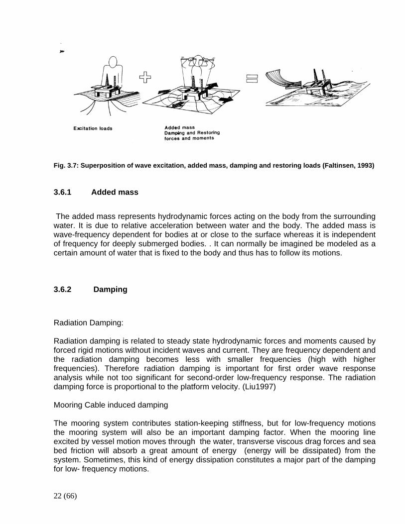
Fig.3.7 Superposition of wave excitation, added mass, damping and restoring loads……………………………………………………………………..22

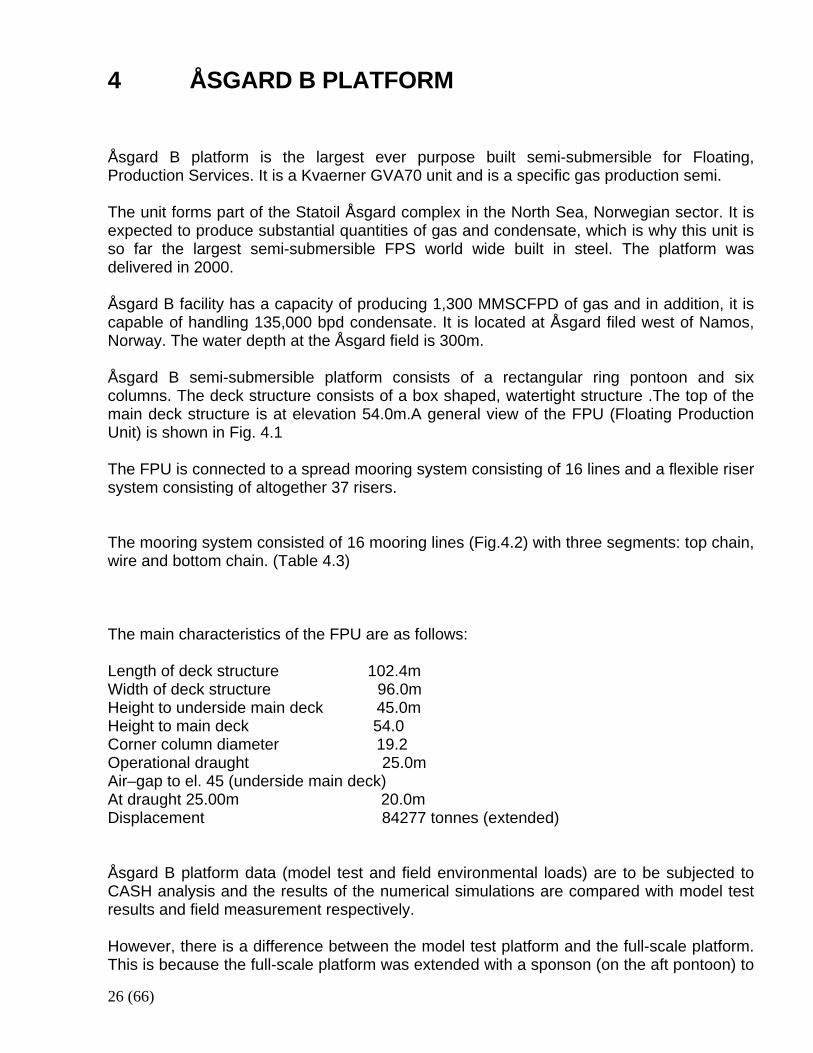
Fig.4.1 Åsgard B semi-submersible platform………………………………………………...27

Fig.4.2 Model test mooring system layout at 0 deg. Heading (plan view) ……………………………………………………………………………….30

Fig.7.1 Work flowchart (for model test and full scale)……………………………………….38

Fig.7.2a Model test and CASH coordinate system comparison……………………………..39

Fig.7.2b Field measurement and CASH coordinate system…………………………………39

Fig.7.3 Full-scale geometric (panel) model…………………………………………………...40

Fig.7.4 Current profile…………………………………………………………………………....42

Fig.8.1 Response Amplitude Operators (RAOs)………………………………………………45

Fig.8.2 Sway response and standard deviation comparison (CASH and model tests 308 and 309) ………………………………………………………....48

Fig.8.3 Response and standard deviation comparison (CASH

and model tests 201,301 and 401 with Sway damping = 1E+ 07 Ns/m) ………………………………………………………………………....52

Fig.8.4 Response and standard deviation comparison (CASH

and reduced measured field data for sea state 2 at 45 deg. heading) ……………………………………………………………………………….....56

Fig.8.5 Response and standard deviation comparison (CASH and reduced measured field data for sea state 5 with Sway damping = 1E+ 07 Ns/m) ……………………………………………………………….58

viii

LIST OF TABLES Table Title Page Table 4.1 Comparison of geometric properties of full-scale and model platforms ………………………………………………………………………...27 Table 4.2a Åsgard B reduced measured field data………………………………………28

Table 4.2b Åsgard B reduced measured field data………………………………………28

Table 4.3 Model test mooring data……………………………………………………….30

Table 4.4 Model tests selected sea-states……………………………………………….31

Table 7.1 Conversion of model tests results to CASH coordinate System……………………………………………………………………………37

Table 8.1 Comparison of hydrostatic and geometric properties……………………….43

Table 8.2 Force coefficient factors………………………………………………………..46

Table 8.3 Calibration test results (tests 312, 311 and 310) ……………………………46

Table 8.4 Calibration test results (410) …………………………………………………...47

Table 8.5 Calibration test results (tests 308 and 309) …………………………………..47

Table 8.6 Comparison of numerical simulations and model test results (tests 201 and 301) ……………………………………………………………..50

Table 8.7 Comparison of numerical simulations and model test results (test 401) …………………………………………………………………………50

Table 8.8 Comparison of numerical simulations and model test results (tests 201 and 301; with Sway damping =1E+ 07 Ns/m) ……………………51

Table 8.9 Comparison of numerical simulations and model test results (test 401; with Sway damping =1E+ 07 Ns/m…………………………………51

Table 8.10 Comparison of numerical simulations and model test results (tests 204 and 304) ……………………………………………………………..53

Table 8.11 Comparison of numerical simulations and model test results (test 404) …………………………………………………………………………53

Table 8.12 Comparison of numerical simulations and reduced measured field data (sea state 2) ………………………………………………………….55

Table 8.13 Comparison of numerical simulations and reduced measured field data (sea state 2) at 45 deg. Heading……………………………………55

Table 8.14 Comparison of numerical simulations and reduced measured field data (sea state 5) ………………………………………………………….57

Table 8.15 Comparison of numerical simulations and reduced measured field data (sea state 5) with Sway damping =1E+ 07 Ns/m…………………57

Table 8.16 Comparison of numerical simulations and reduced measured

field data (sea state 8) …………………………………………………………59

1 (66)

1 INTRODUCTION

1.1 Background Drilling and exploration activities in deepwater require the services of floating offshore structures such as semi-submersibles, FPSO’s, Tension Leg Platforms (TLP), etc. These structures require precise positioning for optimum performance with associated structures such as subsea equipments, risers, mooring etc. In addition they are to resist environmental forces due to the combined effect of wind, current and wave forces in order to maintain good stability for effective field service. It is therefore necessary to estimate the response of these structures to environmental loads when in service. This is necessary during design, construction, towing, operation and maintenance. Free floating structures are known to have motions in six degrees of freedom (free floating or fully coupled), three in translation: surge, sway and heave; and three in rotation: roll, pitch and yaw. While motion in the vertical plane of roll, pitch and heave tend to be relatively stable because of large hydrostatic restoring forces, motions in the horizontal plane of surge sway and yaw derive their restoring forces from stationkeeping systems. Station keeping could be carried out either by mooring system or Dynamic positioning (DP). The analysis and design of mooring systems is of great importance to the overall performance and reliability of an offshore floating structure. It involves determination of the motion, line tensions in the mooring lines, restoring forces, etc. The mooring analysis of a floating platform could be carried out either by computation or model test. Computational analysis is done either in the time domain or in the frequency domain. A fully coupled floating platform is a highly non-linear systems (Liu, 1997).Sources of non-linearity includes viscous drag forces, friction between seabed and mooring lines, nonlinear stretching behavior of lines, changes in line geometry, interaction between line and platform, etc. In the time domain analysis, these nonlinearities can be modeled, and hence the computation is complex and requires great deal of computer memory. In the frequency domain computation however, these nonlinearities are linearised and therefore the computation is simpler and faster. However, the frequency domain analysis does not provide information about the distribution of maximum values; hence some extreme value distributions such as Rayleigh are usually assumed. The model test is also used extensively in platform response predictions and analysis. The results have been found to be good, and are used in calibration of certain important parameters for computational analysis. However, it has a number of disadvantages which include high cost, scale effect, full scale flow simulation, statistical uncertainties, etc. It is still widely used to confirm calculation results. The present industrial practice in mooring analysis is to analyse the low-frequency and wave frequency responses separately, assuming the wave-frequency response not to be affected by the mooring system and thereafter the two responses are combined in some

2 (66)

way (Liu, 1997). This obviously does not fully address the problem of combined response from low-frequency and wave frequency accurately. Most available softwares did not solve these problems in the time domain. For example, MIMOSA carries out mooring analysis of a fully coupled floating system in the frequency domain and in three degrees of freedom. CASH (Coupled Analysis Software for Hydrodynamics) was developed to address the problem of a fully coupled mooring floating platform in the time domain. It can be used to simulate the responses of semi-submersible platforms in a fully-coupled manner i.e. the vessel motions and line dynamics compatible at each time step. It has the advantage of solving the problem in a combined state (low-frequency and wave-frequency) in six degrees of freedom in addition to modeling non-linearities. The program has been verified against other software and good agreements have also been obtained between CASH and model tests. (Liu and Aneljung, 2003) STATOIL has measured the motion responses and line tensions of Åsgard B semi-submersible platform in the North Sea. Åsgard B is a typical GVAC design with ring pontoon and 16 mooring lines, and is so far the largest installed semi-submersible platform in the world.

1.2 Objective and scope of work The main objective of the thesis is to apply CASH in the real environmental conditions for which measurement of the responses of Åsgard B semi-submersible platform are available and compare measured and computed responses (motion, tensions etc).

• Create Hydrodynamic and Mooring model for Åsgard B platform (WADAM,

MIMOSA), • Prepare the input data to CASH

• Perform dynamic analysis using CASH (model tests)

• Calibrate wind , current and wave drift coefficients using Åsgard B model test

results • Perform CASH simulation for Åsgard B model test environmental conditions (3

headings, 2 sea-states in each heading )

• Compare CASH with Åsgard B model tests results (motions, line tensions, etc.) • Analysis of the field measurement data to determine what data are needed • CASH simulation for the field measurements; compare responses (motion, line

tensions, etc) between CASH and measured values.

3 (66)

1.3 Approach

• The approach is to use the model test result to calibrate CASH and the input files; CASH is then used for analysis of the measured field results.

4 (66)

2 OFFSHORE STRUCTURES There are different types of offshore structures used in the offshore industry for exploration and production activities. Some of these are described below:

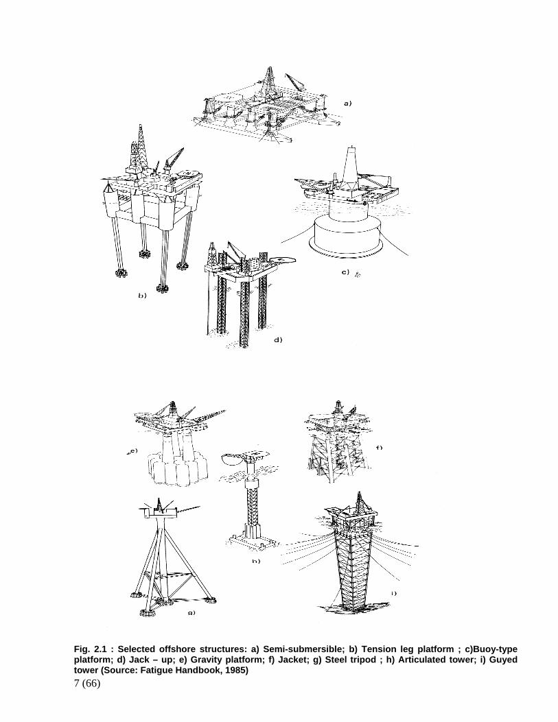
2.1 Semi-submersible Semi-submersible is a type of offshore drilling /production platform. It is constructed of large vertical columns connected to very large pontoons below. This structure supports the drilling deck that accommodates the drilling derrick, equipment, supplies, and crew accommodation. Supply boats and helicopter ferry equipment and personnel between the drill site and shore and it is typically towed to the site and moored to the bottom. It floats high in the water when it is being moved to a site and then the pontoons are flooded to partially submerge the rig so that a majority of its structure is below the water, but the deck is well above the water surface. With only the columns exposed to the wave environment, the semi-submersible is a very stable platform for drilling and production operations. See Fig. 2.1(a) (Randal, 1997)

2.2 Tension Leg Platform (TLP) TLP is an example of compliant structures. These are structures and floating production systems that move with the applied environmental forces resulting from wind, wave and current. They are much lighter in weight and cost less. Tension leg platform is a semi-submersible tethered to the sea floor with vertical legs that are kept in tension by the excess buoyancy of the platform (approximately 15% to 25 %).The tension legs are in sufficient tension that heave, roll, and pitch motions due to waves are essentially eliminated. Sway, surge, yaw motions are experienced but, the tether induced restoring forces are capable of keeping the vessels on station above the well heads. Marine risers carry the petroleum products from the wells to the processing equipment on the deck of the platform and the processed oil and gas is pumped to shore through an export pipeline. See Fig. 2.1(b) (Randal, 1997)

2.3 Guyed Tower Another complaint structure is the guyed tower which is a slender truss-stress structure supported on the sea floor by a spud-can foundation and held upright by multiple wire or chain guy lines. These guy lines connect to anchor piles and are equipped with heavy clump weights between the anchor and tower. The same guy wires also restrain the platform motion during typical operating weather conditions without lifting the clump weights off the bottom. During more extreme weather conditions the guy wires are designed to lift the clump weights off the bottom and the clump weights create larger restoring forces to

5 (66)

resist the larger wave forces. The cost of this type of structure is considerably less than a fixed steel jacketed structure. See Fig 2.1(c) & (i) (Randal, 1997)

2.4 Jack-Up Drilling Rig Jack-up Drilling Rigs are commonly used for drilling shallow water exploration. They can drill to water depth of approximately 122 m. As shown in Fig. 2.1(d), they are designed like a barge with movable elevator legs that can be extended to the sea floor. These rigs are typically towed like the barge to the drilling site with the legs (usually three legs) extended vertically above the barge deck. At the site, the legs are jacked down through the water column and into the sea floor. As the legs engage the sea floor, the drilling deck is raised out of the water and into the air. Deck space provides room for drilling equipment, supplies, and quarters for a crew. Helicopters and ocean supply boats ferry workers and equipment to the rig. The drill deck is well above the height of the highest expected waves. After the drilling is complete, the procedure is reversed and the drilling deck is lowered to the water and the legs are jacked up above the drill deck. The used rig can be towed to another location. (Randal, 1997)

2.5 Gravity Structure This is essentially a concrete structure used for drilling and production. Advantages of these structures are that they have the ability to store oil and construction and testing can be completed before floating the structure and towing it to an offshore location. This type of structure is more tolerant to overloading and degradation due to exposure to sea water than steel platforms. Disadvantages include greater costs than for similar steel structures. More steel is sometimes required for the reinforcing members than required for an equivalent steel jacketed structure. Foundation settlement is expected over the life of the structure which reduces the clearance between the mean water level and the underside of the structure. Although concrete platforms are more expensive, they do offer advantages of lower maintenance and higher deck load. See Fig. 2.1(e) (Randal, 1997).

2.6 Fixed Jacketed Structure A fixed jacketed structure consists of a steel framed tubular structure that is attached to the sea bottom by piles. These piles are driven into the sea floor through pile guides (sleeves) on the outer members of the jacket. The topside structure consists of drilling equipments, production equipments, crew quarters, and eating facilities, gas flare stacks, revolving cranes, survival craft, and a helicopter landing pad. Drilling and production pipes are brought up to topside through conductor guides within the jacket framing and the crude oil and gas travel from the reservoir through the production riser to topside for processing. The produced fluid is then pumped to shore through the export pipeline. The detailed design of the frame varies widely and depends on the requirements of strength, fatigue, and launch procedure. Structural members consists of X and K joints and X and K braced members. The platform phases include design, construction, load-out, launch, installation, piling, and

6 (66)

hook-up before it begins production. The design life of the structure is typically 10-25 years. This is followed by the requirement to remove and dispose of the platform once the reservoir is depleted. Launching of these structures is usually accomplished with barges. Some structures are floated off the barge and righted using barge cranes and others are designed with floatation to be self righting. Since these structures are made of steel, the effects of corrosion must be considered due to its exposure to the ocean environment. Anodic and cathodic protection systems are employed and maintained to protect against corrosion of the structure. Fig. 2.1 (f) (Randal, 1997). An alternative to the conventional truss-work platform, steel or concrete tripod platforms have been suggested for deep water applications, Fig. 2.1 (g). The use of inclined legs makes the global transfer of wave loads to the seafloor very effective, mainly by axial forces.

2.7 Articulated Tower and Single Anchor Leg Moored Systems

For the development of small reservoirs in water depth up to about 200m, an articulated column or a single anchor leg storage and tanker system can be used in relatively calm weather areas. Crude oil is moved up the articulated tower and transferred to the tethered tanker for processing and storage. A shuttle tanker is brought alongside to receive the processed oil and transport it to shore. The single anchor leg mooring (SALM) system uses a yoke structure, buoyancy tank, and tensioned riser to moor a tanker. Processing and storage facilities are housed in the tanker and oil export is accomplished with a shuttle tanker or an export oil pipelines. See Fig 2.1 (h) (Randal, 1997).

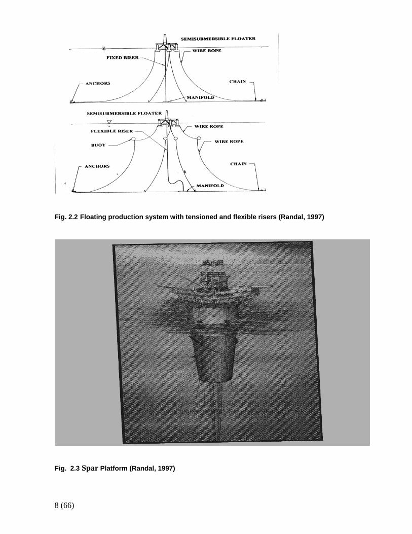
2.8 Floating platform versus Fixed platform An economical production system for small reservoirs is the floating production system (FPS) that consists of a converted or newly built semi-submersible that is moored to the seafloor using a catenary mooring system. Connection to the oil reservoir is through a rigid tensioned vertical multiple production risers or through flexible risers. This system supports only a relatively small deck load that limits the oil processing options compared to the capabilities of a fixed platform. The compliance of the system and the catenary mooring system create some risks such as damaged risers and moving to far off station in severe environmental conditions. The platform has no oil storage capabilities and the vessel motions in severe weather conditions can limit or degrade the processing operations. Nonetheless, the floating production systems provides an economic means for working small reservoirs that require only limited processing facelifts. See Fig 2.2 (Randal, 1997).

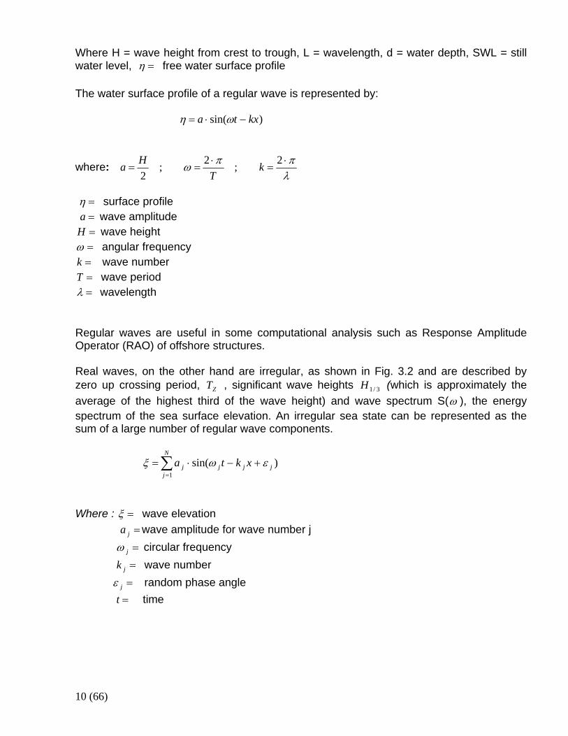
2.9 Spar Platform A new compliant structure being designed and developed for deep water offshore installations is called spar platform (Fig. 2.3).Its response characteristics in deep water make it a viable possibility for ( deepwater more than 1000 m depth) petroleum production. (Randal, 1997).

7 (66)

Fig. 2.1 : Selected offshore structures: a) Semi-submersible; b) Tension leg platform ; c)Buoy-type platform; d) Jack – up; e) Gravity platform; f) Jacket; g) Steel tripod ; h) Articulated tower; i) Guyed tower (Source: Fatigue Handbook, 1985)

8 (66)

Fig. 2.2 Floating production system with tensioned and flexible risers (Randal, 1997)

Fig. 2.3 Spar Platform (Randal, 1997)

9 (66)

3 ENVIRONMENTAL LOADS AND FORCES ON OFFSHORE STRUCTURES

Environmental forces on offshore structures are mainly caused by the combined actions of waves, current and wind. Waves induce forces such as wave frequency, low frequency and wave drift forces, while wind could induce both steady and time varying loads. Currents are mostly treated as steady direct forces, however, its variation with water depth is most significant. Environmental data are usually gathered for the proposed offshore field location. This is used in the computation of the environmental loads. Extensive meteorological data are needed and these data are projected statistically over a period that covers the entire lifespan of the offshore structure. This is done to obtain the required responses of the structure. For waves, data such as significant wave height, zero crossing period or crest periods and headings are very important, while wind speed and direction are required in the case of wind. Current data is of utmost importance. Wave spectra must also be used as a start in all calculations. A suitable wave spectrum model is chosen representing an appropriate density distribution of the sea waves at the site under consideration (Chakrabarti, 1987).The choice is made based on the fetch, wind and other meteorological conditions of this site. Examples of standard wave spectrum include JONSWAP, PM, etc. Environmental forces could either be computed or obtained through model test. Depending on the response of interest, it is important that both computation and model tests are carried out. In most cases, the model test is used to confirm the calculations.

3.1 Waves In offshore design, waves are usually classed as regular and irregular waves. Regular waves are based on linear wave theory with highly simplified wave analysis by a number of assumptions such as constant water depth etc. A typical regular wave is shown in Fig 3.1.

Fig. 3.1: Regular waves

10 (66)

Where H = wave height from crest to trough, L = wavelength, d = water depth, SWL = still water level, =η free water surface profile The water surface profile of a regular wave is represented by:

)sin( kxta −⋅= ωη

where: λππω ⋅

=⋅

==2;2;

2k

THa

=η surface profile =a wave amplitude

=H wave height =ω angular frequency =k wave number =T wave period =λ wavelength

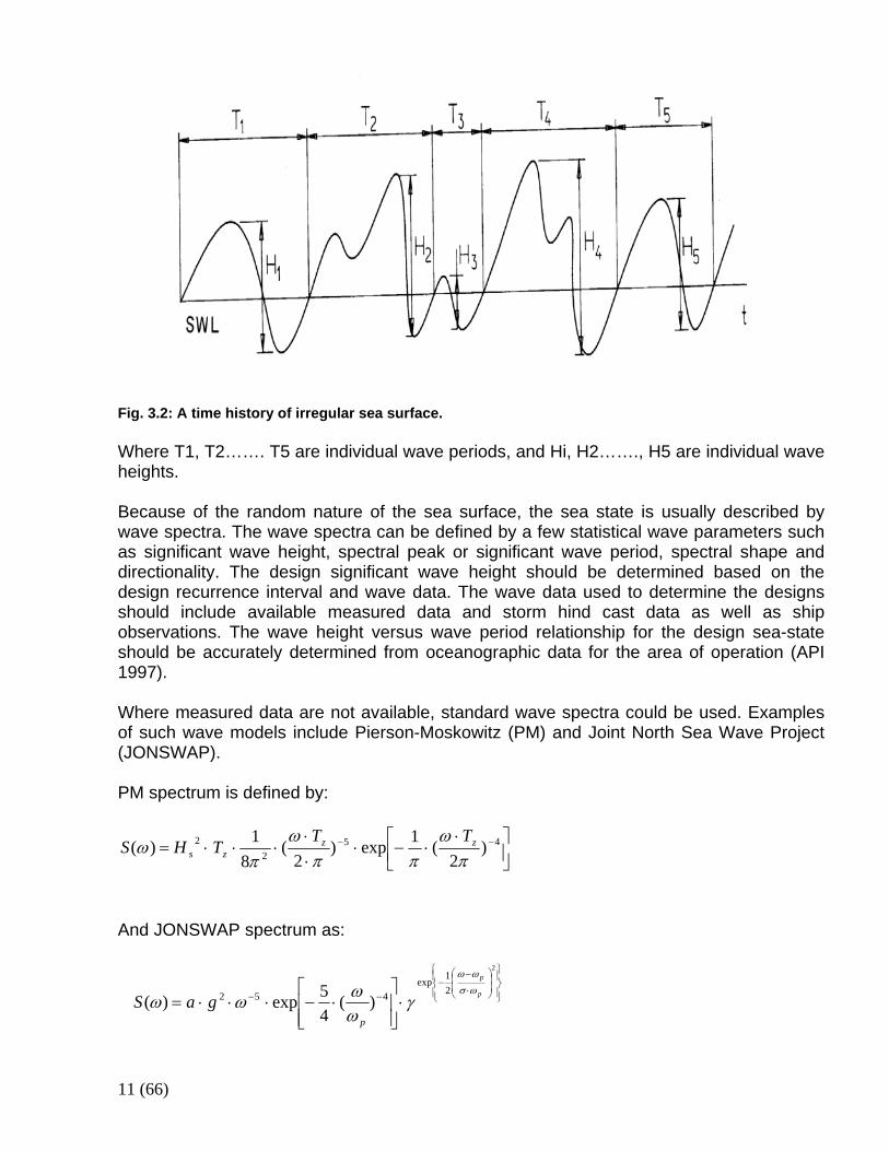
Regular waves are useful in some computational analysis such as Response Amplitude Operator (RAO) of offshore structures. Real waves, on the other hand are irregular, as shown in Fig. 3.2 and are described by zero up crossing period, ZT , significant wave heights 3/1H (which is approximately the average of the highest third of the wave height) and wave spectrum S(ω ), the energy spectrum of the sea surface elevation. An irregular sea state can be represented as the sum of a large number of regular wave components.

∑=

+−⋅=N

jjjjj xkta

1

)sin( εωξ

Where : =ξ wave elevation =ja wave amplitude for wave number j =jω circular frequency =jk wave number =jε random phase angle =t time

11 (66)

Fig. 3.2: A time history of irregular sea surface. Where T1, T2……. T5 are individual wave periods, and Hi, H2……., H5 are individual wave heights. Because of the random nature of the sea surface, the sea state is usually described by wave spectra. The wave spectra can be defined by a few statistical wave parameters such as significant wave height, spectral peak or significant wave period, spectral shape and directionality. The design significant wave height should be determined based on the design recurrence interval and wave data. The wave data used to determine the designs should include available measured data and storm hind cast data as well as ship observations. The wave height versus wave period relationship for the design sea-state should be accurately determined from oceanographic data for the area of operation (API 1997). Where measured data are not available, standard wave spectra could be used. Examples of such wave models include Pierson-Moskowitz (PM) and Joint North Sea Wave Project (JONSWAP). PM spectrum is defined by:

⎥⎦⎤

⎢⎣⎡ ⋅

⋅−⋅⋅⋅

⋅⋅⋅= −− 452

2 )2

(1exp)2

(8

1)(π

ωππ

ωπ

ω zzzs

TTTHS

And JONSWAP spectrum as:

⎪⎭

⎪⎬⎫

⎪⎩

⎪⎨⎧

⎟⎟⎠

⎞⎜⎜⎝

⎛

⋅

−−

−− ⋅⎥⎥⎦

⎤

⎢⎢⎣

⎡⋅−⋅⋅⋅=

2

21exp

452 )(45exp)( p

p

p

gaSωσ

ωω

γωωωω

12 (66)

Where : =)(ωS wave spectrum =zT zero upcrossing period =sH significant wave height =ω angular frequency =pω peak angular frequency =γ peak enhancement factor =a philip’s constant

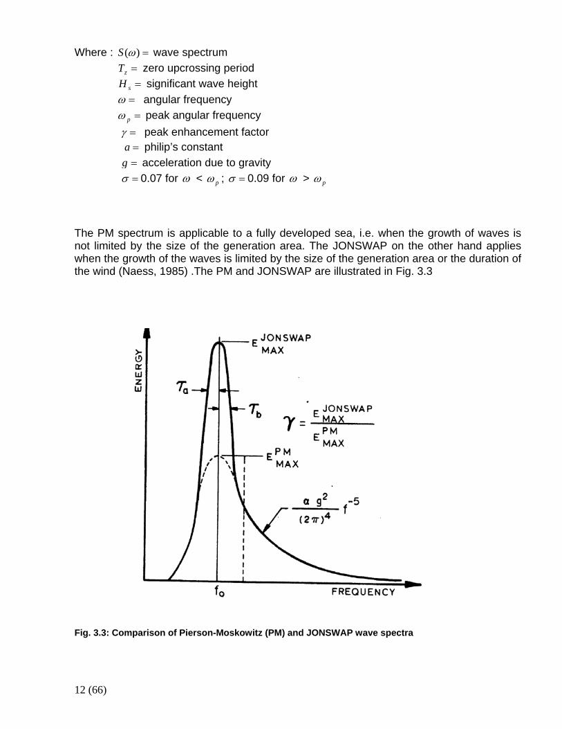
=g acceleration due to gravity =σ 0.07 for ω < pω ; =σ 0.09 for ω > pω The PM spectrum is applicable to a fully developed sea, i.e. when the growth of waves is not limited by the size of the generation area. The JONSWAP on the other hand applies when the growth of the waves is limited by the size of the generation area or the duration of the wind (Naess, 1985) .The PM and JONSWAP are illustrated in Fig. 3.3

Fig. 3.3: Comparison of Pierson-Moskowitz (PM) and JONSWAP wave spectra

13 (66)

3.1.1 Wave Induced forces

Wave forces on circular members of offshore structures could be computed in three different ways:

i) Froude-Krylov theory

ii) Diffraction theory

iii) Morison equation

A first approximation of the forces that excite the motion of a floating body are called Froude-Krylov forces. They results from the integration over the body surface of the pressure which would exist in the wave system in the absence of the floating body. .The Froude-Krylov theory can be applied when the drag force is small and the inertial forces predominates but the structure is still relatively small. It utilizes the incident wave pressure–area method on the surface of the structure to compute the force. It assumes that the wave properties are unaffected by the presence of structure. The second component of the exciting force is caused by the diffraction of the incident waves due to the presence of the floating structure. This usually occurs when the size of the structure is compatible to the wavelength; the presence of the structure is expected to alter the wave field in the vicinity of the structure. In this case, the diffraction of the wave from the surface if the structure should be taken into account in the evaluation of the wave forces, this is generally known as diffraction theory (Chakrabarti, 1987). The Morison equation assumes the force to be composed of inertia and drag forces linearly added together. The components involve an inertia (or mass) ( MC ) coefficient and a drag ( DC ) coefficient which have to be determined experimentally and are dependent on many parameters such as Reynolds number ( eR ) and the surface roughness. The Morison equation is applicable when the drag force is significant. This is usually the case when a structure is small compared to the wavelength. The hydrodynamic force per unit length on a body can be expressed by Morison’s equation as follows:

XXDCXCDdF DM&&&& ⋅⋅⋅⋅+⋅⋅⋅⋅=

24

2 ρπρ

Where :

=X&& acceleration of undisturbed fluid field

14 (66)

=X& velocity of undisturbed fluid filed =ρ density of seawater =D diameter of cylinder

=DC drag coefficient =MC mass coefficient

Wave forces induce motion in the offshore floating structures and forces on the mooring system. Interaction between ocean waves and floating vessels results in the following forces acting on the vessels: (a) First order forces that oscillate at the wave frequency inducing first order motions known as high frequency or wave frequency motions. This has an important contribution to the total mooring loads and the resulting wave frequency motion is in six degrees of freedom: surge, sway, heave, roll, pitch and yaw. (b) Steady components of the second order forces known as mean wave drift forces. The mean forces are of great importance for the mean offset of the platform. For a surface body, a major contribution to the horizontal mean wave drift force is the relative vertical motion between the structure and the waves. This causes some of the body surface to be in the water and part of the time out of the water, which results in a non-zero mean pressure. If the relative vertical motion differs around the waterline, the result is a non-zero mean force. This occurs for large volume structures where incident waves are modified by the structure. However, for long wavelengths relative to the cross-sectional dimensions, the body will not disturb the wave field. This means that the wave drift force become negligible for these types of structure (Rosen and Brannström, 1999).Another contribution to wave drift forces is the constant force from the sums and differences non-linear interaction of waves of different frequencies. These waves could be regular or random. (Chakrabarti, 1990) (c) Second order slowly varying forces with frequencies below wave frequencies induce second order motions known as low frequency motions. These forces are small compared to the first order. However, since they tend to occur at frequencies equivalent to the eigen period of the moored body, they may generate large resonant motions. Hence, they are only significant in the horizontal degrees of freedom: surge, sway and yaw .There forces have frequencies that equal the differences of the regular component wave frequencies. Consider an idealised sea state consisting of two wave components of circular frequencies 1ω and 2ω ,an approximation for the x-component of the velocity can be written as : )cos()cos( 222111 εωεω +++= tAtAVx The quadratic pressure term in the Bernoulli’s equation can be expresses as:

)(2

222zyx VVV ++−

ρ

substituting the velocity expression in the Bernoulli’s equation results in:

15 (66)

[ ]

[ ]212121

21212122

22

11

21

22

21

2

)(cos

)(cos)22cos(2

)22cos(22222

εεωω

εεωωεωεωρρ

++++⎥⎥⎥

⎦

⎤

⎢⎢⎢

⎣

⎡−+−++++++−=−

tAA

tAAtA

tAAA

Vx

This expression showed the presence of a constant pressure term, a pressure term that oscillates with the difference frequency ( 1ω - 2ω ) and also terms oscillating with higher frequencies 2 1ω , 2 2ω and ( 1ω + 2ω ). The constant term will contribute to the mean drift forces, while the non-linear difference terms produce slowly varying excitation forces. (Rosen and Brannström, 1999).The sum terms give frequencies much above the resonance frequencies of the floating platform, so they can not excite the platform motion

3.2 Wind Wind is a significant design factor. The wind conditions used in design should be appropriately determined from collected data and should be consistent with other environmental parameters assumed to occur simultaneously. The design wind speed should refer to an elevation of 10 meters above still water level. Two methods are generally used to assess effects of wind for design. These include: 1. Wind forces are treated as constant and calculated on the basis of 1-minute average velocity. 2. Fluctuating wind force is calculated on the basis of a steady component, based on the 1-hour average velocity for one-hour simulation and two-hour average velocity for two-hour simulation, etc. plus a time varying component calculated from a suitable empirical wind gust spectrum. This is also known as low–frequency wind force. The choice of method depends on the system parameters and goals of the analysis. The forces due to wind may be determined by using wind tunnel or towing tank model test data or calculations. The steady state force due to wind acting on a moored floating unit can be determined using the equation below (API, 1997): 2).(. whsww VACCCF ∑= =wF wind force, (N)

=wC 42 /sec615.0 mN =sC shape coefficient =hC height coefficient

=A vertical projected area of each surface exposed to the wind, 2m

16 (66)

=wV design wind speed , m/sec. Low – frequency wind forces are normally computed from an empirical wind energy spectrum.

3.3 Current

The most common categories of currents are: a) Tidal currents (associated with astronomical tides) (b) circulated currents (associated with oceanic-scale circulation patterns) (c) storm-generated currents (d) loop and eddy currents. The vector sum of these currents is the total current and the speed and direction of the current at specified elevations are represented by a current profile. The total current profile associated with the sea state producing extreme waves is usually specified for mooring design. Current forces are normally treated as steady state forces in a mooring analysis. They can be estimated by model tests or calculations. Current forces on a semi-submersible hull can be computed by the following equation (API, 1997)

2)..( cfdcdsscs VACACCF +=

=csF current force, N =ssC current force coefficient for semi submersible hulls = 42 /sec62.515 mN =dC drag coefficient =cA summation of total projected areas of all cylindrical members below the waterline 2m =fA summation of projected areas of all members having flat surfaces below the

waterline 2m Environmental forces are usually combined calculated in the following three distinct frequency bands to evaluate their effects on the system: 1. Steady forces such as wind, current and wave drift forces are set constant in magnitude and direction for the duration of interest. 2. Low frequency cyclic loads can excite the platform at its natural periods in surge, sway, and yaw 3. Wave frequency cyclic loads are large in magnitude and are mostly major contributors to platform member forces and mooring forces.

17 (66)

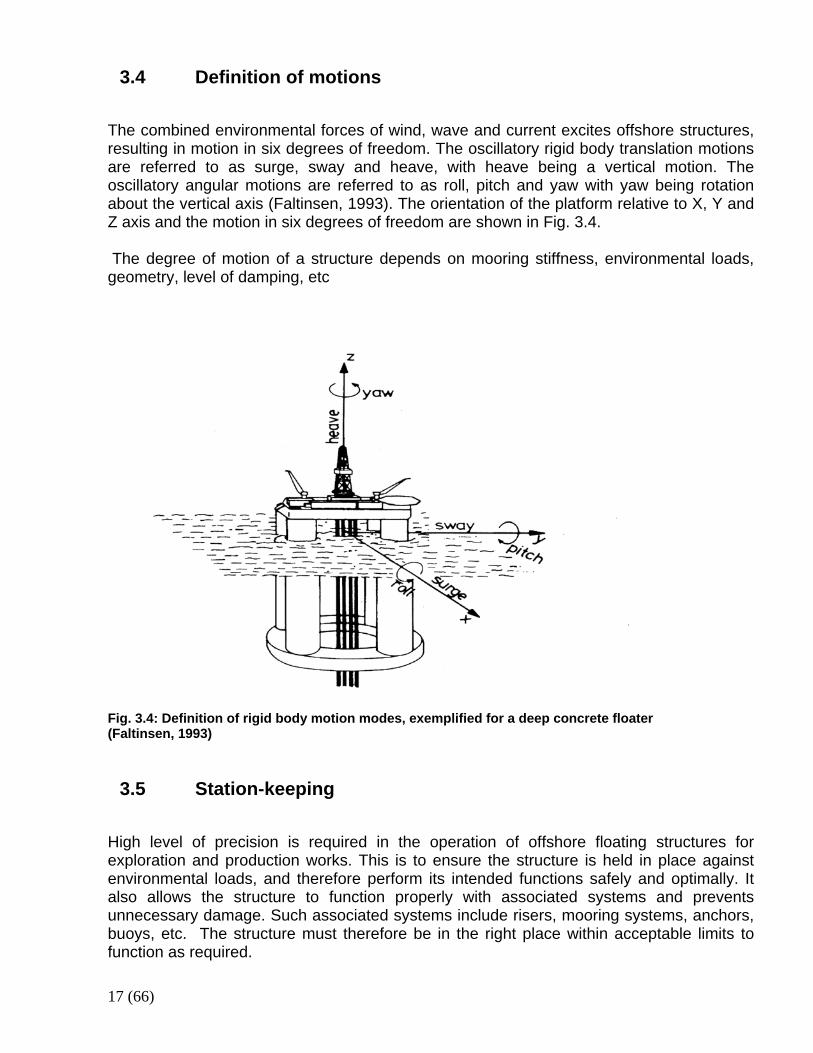
3.4 Definition of motions

The combined environmental forces of wind, wave and current excites offshore structures, resulting in motion in six degrees of freedom. The oscillatory rigid body translation motions are referred to as surge, sway and heave, with heave being a vertical motion. The oscillatory angular motions are referred to as roll, pitch and yaw with yaw being rotation about the vertical axis (Faltinsen, 1993). The orientation of the platform relative to X, Y and Z axis and the motion in six degrees of freedom are shown in Fig. 3.4. The degree of motion of a structure depends on mooring stiffness, environmental loads, geometry, level of damping, etc

Fig. 3.4: Definition of rigid body motion modes, exemplified for a deep concrete floater (Faltinsen, 1993)

3.5 Station-keeping

High level of precision is required in the operation of offshore floating structures for exploration and production works. This is to ensure the structure is held in place against environmental loads, and therefore perform its intended functions safely and optimally. It also allows the structure to function properly with associated systems and prevents unnecessary damage. Such associated systems include risers, mooring systems, anchors, buoys, etc. The structure must therefore be in the right place within acceptable limits to function as required.

18 (66)

Dynamic Positioning (DP) and Mooring systems are the two common methods of station- keeping. 3.5.1 Dynamic Positioning (DP) System

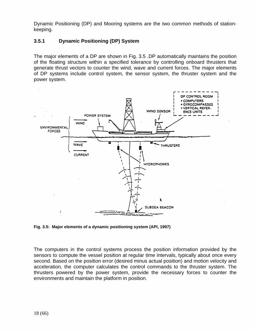
The major elements of a DP are shown in Fig. 3.5 .DP automatically maintains the position of the floating structure within a specified tolerance by controlling onboard thrusters that generate thrust vectors to counter the wind, wave and current forces. The major elements of DP systems include control system, the sensor system, the thruster system and the power system.

Fig. 3.5: Major elements of a dynamic positioning system (API, 1997) The computers in the control systems process the position information provided by the sensors to compute the vessel position at regular time intervals, typically about once every second. Based on the position error (desired minus actual position) and motion velocity and acceleration, the computer calculates the control commands to the thruster system. The thrusters powered by the power system, provide the necessary forces to counter the environments and maintain the platform in position.

19 (66)

3.5.2 Mooring Systems

Mooring system consists of a number of cables which are attached to the floating structure at different locations with the lower end of the cable anchored to the sea bed. Mooring systems provide restoring forces in the horizontal plane (surge, sway and yaw). Typically, a mooring system could be a Single Point Mooring (SPM) or a spread mooring. In a spread mooring system, several pre-tensioned anchor lines are arrayed around the structure to hold the structure in the desired location. The cables are made of chain, rope or a combination of both. Spread mooring is most common with floating drilling systems, especially semi-submersibles. Fig. 3.6

Fig. 3.6: Major elements of spread moorings (API, 1997)

20 (66)

Single point mooring on the other hand is used primarily for tankers and other ship type structures. There are basically three types of single point mooring systems: Turret mooring, where a number of mooring legs are attached to a turret that is essentially part of the vessel to be moored. The turret includes bearings that allow the vessel to rotate around the anchor legs. The turret can be mounted externally from the vessel bow or stern with appropriate reinforcements. Catenary Anchor Leg Mooring (CALM) is another type of single point moorings. It consists of a large buoy that supports a number of catenary chain legs anchored to the sea floor. Riser systems or flow lines are that emerge from the sea floor are attached to the underside of the CALM buoy. Single Anchor Leg Mooring, (SALM), employs a vertical riser system that has a large amount of buoyancy near the surface and sometimes on the surface that is held by a pretension riser. The vertical buoyancy force acting on the top of the riser functions as an inverted pendulum. When the system is displaced to the side, the pendulum action tends to restore the riser to the vertical position. (API, 1997)

3.6 Response analysis of a Moored floating platform Response analysis involve solving the differential equation of motion in six degrees of freedom (surge, sway, heave, roll, pitch and yaw) for mooring line tension, platform motion/offsets, restoring forces, anchor loads etc. due to the combined environmental forces of waves, wind and current. The analysis is performed for intact condition (all lines are intact), damaged condition (at least one line broken) and transient condition (platform subjected to transient motion after a mooring line breakage before it settles at the new equilibrium position). Generally speaking, the response of a mooring system to mean forces of current, mean wind and wave drift forces are predicted by static equilibrium of the catenary system. Low frequency motions due to wind and waves can also be predicted by static catenary analysis in each offset position. However, wave frequency response is usually predicted by the following methods:

a) Quasi-static analysis: In this approach, the dynamic wave loads are taken into consideration by statically offsetting the platform by an appropriately defined wave induced motion. Vertical fairlead motions and dynamic effects associated with mass, damping, and fluid acceleration are neglected. This method is widely used for temporary mooring line design and preliminary studies of permanent moorings with higher factors of safety.

b) Dynamic analysis: Dynamic analysis accounts for the time varying effects due to mass, damping, and fluid acceleration. In this approach, the time varying fairlead motions are calculated from the vessel’s surge, sway, heave, pitch, roll, and yaw. motions. Two methods are commonly employed in dynamic mooring analysis. These

21 (66)

are frequency domain and time domain analysis. A fully coupled floating platform is a highly non-linear systems (Liu, 1997).Sources of non-linearity includes viscous drag forces, friction between seabed and mooring lines, nonlinear stretching behavior of lines, changes in line geometry, interaction between line and platform, etc. In time domain analysis, these nonlinearities are modeled, and hence the computation is complex and requires great deal of computer memory. In frequency domain computation however, these nonlinearities are eliminated either by direct linearization or by an iterative linearisation and therefore the computation is simpler and faster.

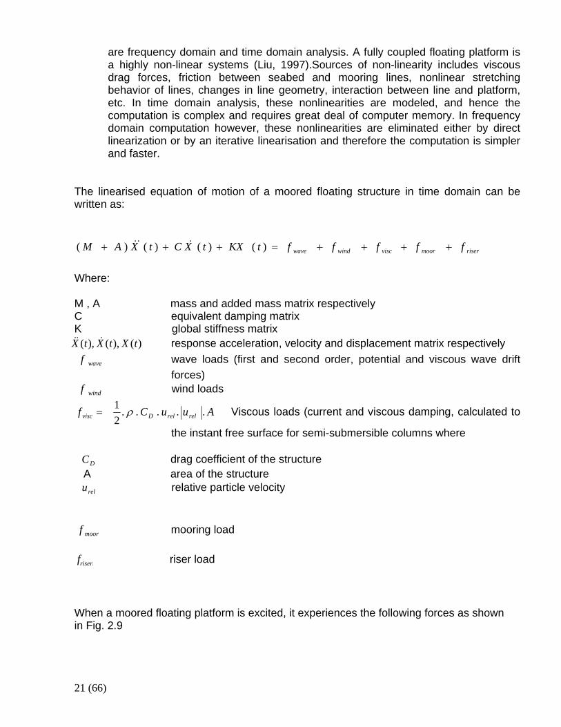
The linearised equation of motion of a moored floating structure in time domain can be written as:

risermoorviscwindwave ffffftKXtXCtXAM ++++=+++ )()()()( &&&

Where: M , A mass and added mass matrix respectively C equivalent damping matrix K global stiffness matrix

)(),(),( tXtXtX &&& response acceleration, velocity and displacement matrix respectively

wavef wave loads (first and second order, potential and viscous wave drift forces)

windf wind loads

AuuCf relrelDvisc .....21 ρ= Viscous loads (current and viscous damping, calculated to

the instant free surface for semi-submersible columns where DC drag coefficient of the structure A area of the structure relu relative particle velocity

moorf mooring load

riserrf riser load When a moored floating platform is excited, it experiences the following forces as shown in Fig. 2.9

22 (66)

Fig. 3.7: Superposition of wave excitation, added mass, damping and restoring loads (Faltinsen, 1993) 3.6.1 Added mass

The added mass represents hydrodynamic forces acting on the body from the surrounding water. It is due to relative acceleration between water and the body. The added mass is wave-frequency dependent for bodies at or close to the surface whereas it is independent of frequency for deeply submerged bodies. . It can normally be imagined be modeled as a certain amount of water that is fixed to the body and thus has to follow its motions. 3.6.2 Damping

Radiation Damping: Radiation damping is related to steady state hydrodynamic forces and moments caused by forced rigid motions without incident waves and current. They are frequency dependent and the radiation damping becomes less with smaller frequencies (high with higher frequencies). Therefore radiation damping is important for first order wave response analysis while not too significant for second-order low-frequency response. The radiation damping force is proportional to the platform velocity. (Liu1997) Mooring Cable induced damping The mooring system contributes station-keeping stiffness, but for low-frequency motions the mooring system will also be an important damping factor. When the mooring line excited by vessel motion moves through the water, transverse viscous drag forces and sea bed friction will absorb a great amount of energy (energy will be dissipated) from the system. Sometimes, this kind of energy dissipation constitutes a major part of the damping for low- frequency motions.

23 (66)

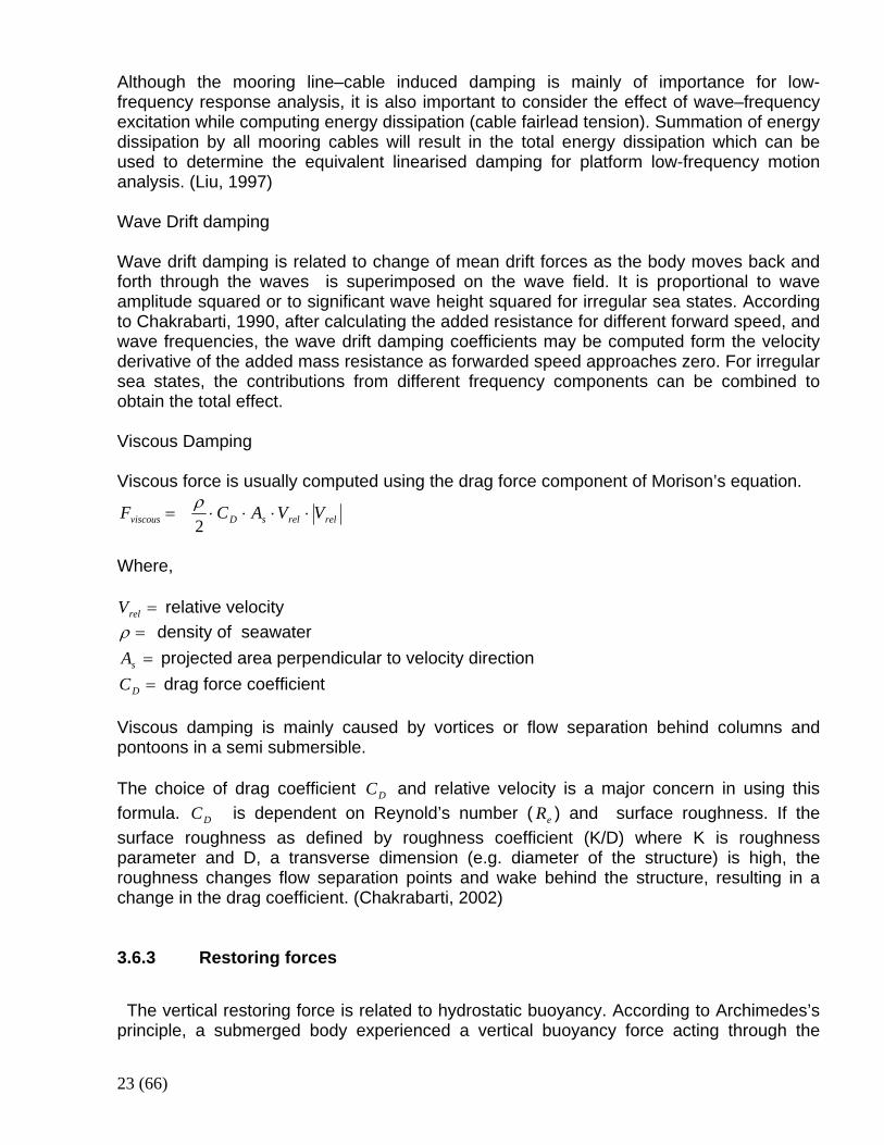
Although the mooring line–cable induced damping is mainly of importance for low-frequency response analysis, it is also important to consider the effect of wave–frequency excitation while computing energy dissipation (cable fairlead tension). Summation of energy dissipation by all mooring cables will result in the total energy dissipation which can be used to determine the equivalent linearised damping for platform low-frequency motion analysis. (Liu, 1997) Wave Drift damping Wave drift damping is related to change of mean drift forces as the body moves back and forth through the waves is superimposed on the wave field. It is proportional to wave amplitude squared or to significant wave height squared for irregular sea states. According to Chakrabarti, 1990, after calculating the added resistance for different forward speed, and wave frequencies, the wave drift damping coefficients may be computed form the velocity derivative of the added mass resistance as forwarded speed approaches zero. For irregular sea states, the contributions from different frequency components can be combined to obtain the total effect. Viscous Damping Viscous force is usually computed using the drag force component of Morison’s equation.

relrelsDviscous VVACF ⋅⋅⋅⋅=2ρ

Where,

=relV relative velocity =ρ density of seawater =sA projected area perpendicular to velocity direction =DC drag force coefficient

Viscous damping is mainly caused by vortices or flow separation behind columns and pontoons in a semi submersible. The choice of drag coefficient DC and relative velocity is a major concern in using this formula. DC is dependent on Reynold’s number ( eR ) and surface roughness. If the surface roughness as defined by roughness coefficient (K/D) where K is roughness parameter and D, a transverse dimension (e.g. diameter of the structure) is high, the roughness changes flow separation points and wake behind the structure, resulting in a change in the drag coefficient. (Chakrabarti, 2002) 3.6.3 Restoring forces

The vertical restoring force is related to hydrostatic buoyancy. According to Archimedes’s principle, a submerged body experienced a vertical buoyancy force acting through the

24 (66)

centre of the displaced water volume (centre of buoyancy) and this force is equal to the weight of the fluid displaced. The buoyancy forces therefore provide large hydrostatic restoring forces in the vertical plane where heave, roll, and pitch motions are present. In the horizontal plane of surge, sway and yaw, however, the restoring forces are due to mooring or dynamic positioning systems and production risers.

3.7 Mooring System Analysis Problems Solving the equation of motion of a moored floating structure is a complex and time consuming task. There are a number of factors that make the problem difficult to solve. Some of these are highlighted below:

i) Non- Linearity: According to Liu 1997, a moored floating platform is a highly non-linear system. There are many sources of non-linearity including viscous drag forces, second order low frequency wave excitation forces, interaction between cables and platform, changes in line shape geometry, nonlinear stretching behavior of the line, sea bed-cable friction, vortex induced vibration, etc. The non-linearity makes the computation somewhat difficult.

ii) Damping: There are four different types of damping associated with moored

platform. These include radiation damping, mooring cable induced damping, wave drift damping, and viscous damping. Damping absorbs energy from the system. Modeling the entire damping phenomenon correctly is rather complicated and this largely contributes to the complexity involved in mooring system analysis.

iii) Another major problem in mooring analysis is the coexistence of both wave –

frequency and low-frequency excitation forces. Solving the equation of motion for this combined extreme response is difficult. According to Liu 1997, the present industry practice is to analyse the low-frequency and wave frequency responses separately, assuming the wave-frequency response not to be affected by the mooring system. Thereafter the two responses are combined in some way. This procedure may be somewhat conservative.

CASH program solves the equation of motion in the time domain and combines low frequency and wave frequency response at the same time, and therefore addresses most of these problems.

3.8 Model Tests Model tests are required during the final stage of design to compensate for the limitations of computational analysis. Model test may be used either as a self–contained program for determining the responses of a particular floating unit or as a verification of analytical

25 (66)

predictions of the responses. Other model tests usually conducted are ocean basin test (to establish wave drift coefficients and damping level) and wind tunnel test (wind and current drag coefficients).These coefficients form part of inputs to the analytical response prediction. API 1997 states the primary objectives of model tests as follows:

a) To determine maximum responses for design purpose for example motions, line tension, forces at mooring interfaces etc

b) To quantify important parameters and thereby to calibrate computer programs c) To confirm that no important facet of the operation has been overlooked.

The model test however has a number of disadvantages which include high cost, scale effect, statistical uncertainties, etc. Therefore numerical predictions and model experimental results are complementary to each other. In order to obtain realistic results from model tests, it is important to select the proper vessel and mooring line model scales and testing facilities (size and depth of model basin, wave, wind, and current generating capability).Care should be taken to ensure that the character of the flow in the model test is the same as the character of the flow for the full-scale unit.

26 (66)

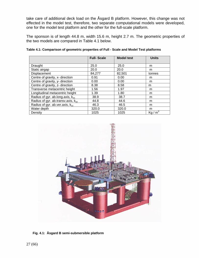
4 ÅSGARD B PLATFORM Åsgard B platform is the largest ever purpose built semi-submersible for Floating, Production Services. It is a Kvaerner GVA70 unit and is a specific gas production semi. The unit forms part of the Statoil Åsgard complex in the North Sea, Norwegian sector. It is expected to produce substantial quantities of gas and condensate, which is why this unit is so far the largest semi-submersible FPS world wide built in steel. The platform was delivered in 2000. Åsgard B facility has a capacity of producing 1,300 MMSCFPD of gas and in addition, it is capable of handling 135,000 bpd condensate. It is located at Åsgard filed west of Namos, Norway. The water depth at the Åsgard field is 300m. Åsgard B semi-submersible platform consists of a rectangular ring pontoon and six columns. The deck structure consists of a box shaped, watertight structure .The top of the main deck structure is at elevation 54.0m.A general view of the FPU (Floating Production Unit) is shown in Fig. 4.1 The FPU is connected to a spread mooring system consisting of 16 lines and a flexible riser system consisting of altogether 37 risers. The mooring system consisted of 16 mooring lines (Fig.4.2) with three segments: top chain, wire and bottom chain. (Table 4.3) The main characteristics of the FPU are as follows: Length of deck structure 102.4m Width of deck structure 96.0m Height to underside main deck 45.0m Height to main deck 54.0 Corner column diameter 19.2 Operational draught 25.0m Air–gap to el. 45 (underside main deck) At draught 25.00m 20.0m Displacement 84277 tonnes (extended) Åsgard B platform data (model test and field environmental loads) are to be subjected to CASH analysis and the results of the numerical simulations are compared with model test results and field measurement respectively. However, there is a difference between the model test platform and the full-scale platform. This is because the full-scale platform was extended with a sponson (on the aft pontoon) to

27 (66)

take care of additional deck load on the Åsgard B platform. However, this change was not effected in the model test, therefore, two separate computational models were developed, one for the model test platform and the other for the full-scale platform. The sponson is of length 44.8 m, width 15.6 m, height 2.7 m. The geometric properties of the two models are compared in Table 4.1 below. Table 4.1: Comparison of geometric properties of Full - Scale and Model Test platforms

Full- Scale Model test Units

Draught 25.0 25.0 m Static airgap 20.0 20.0 m Displacement 84,277 82,501 tonnes Centre of gravity, x- direction 0.91 0.00 m Centre of gravity, y- direction 0.00 0.00 m Centre of gravity, z- direction 8.38 8.58 m Transverse metacentric height 1.56 1.97 m Longitudinal metacentric height 1.39 1.80 m Radius of gyr. ab.long.axis, kxx 38.9 38.7 m Radius of gyr. ab.transv.axis, kyy 44.8 44.6 m Radius of gyr. ab.ver.axis, kzz 46.3 46.5 m Water depth 320.0 320.0 m Density 1025 1025 Kg / m3

Fig. 4.1: Åsgard B semi-submersible platform

28 (66)

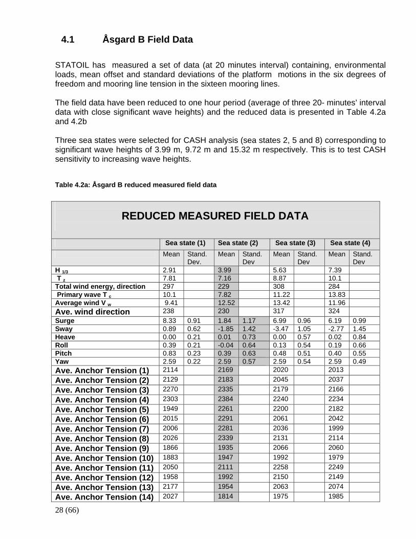
4.1 Åsgard B Field Data STATOIL has measured a set of data (at 20 minutes interval) containing, environmental loads, mean offset and standard deviations of the platform motions in the six degrees of freedom and mooring line tension in the sixteen mooring lines. The field data have been reduced to one hour period (average of three 20- minutes’ interval data with close significant wave heights) and the reduced data is presented in Table 4.2a and 4.2b Three sea states were selected for CASH analysis (sea states 2, 5 and 8) corresponding to significant wave heights of 3.99 m, 9.72 m and 15.32 m respectively. This is to test CASH sensitivity to increasing wave heights. Table 4.2a: Åsgard B reduced measured field data REDUCED MEASURED FIELD DATA

Sea state (1) Sea state (2) Sea state (3) Sea state (4) Mean Stand.

Dev. Mean Stand.

Dev Mean Stand.

Dev Mean Stand.

Dev H 1/3 2.91 3.99 5.63 7.39 T z 7.81 7.16 8.87 10.1 Total wind energy, direction 297 229 308 284 Primary wave T c 10.1 7.82 11.22 13.83 Average wind V w 9.41 12.52 13.42 11.96 Ave. wind direction 238 230 317 324 Surge 8.33 0.91 1.84 1.17 6.99 0.96 6.19 0.99 Sway 0.89 0.62 -1.85 1.42 -3.47 1.05 -2.77 1.45 Heave 0.00 0.21 0.01 0.73 0.00 0.57 0.02 0.84 Roll 0.39 0.21 -0.04 0.64 0.13 0.54 0.19 0.66 Pitch 0.83 0.23 0.39 0.63 0.48 0.51 0.40 0.55 Yaw 2.59 0.22 2.59 0.57 2.59 0.54 2.59 0.49 Ave. Anchor Tension (1) 2114 2169 2020 2013 Ave. Anchor Tension (2) 2129 2183 2045 2037 Ave. Anchor Tension (3) 2270 2335 2179 2166 Ave. Anchor Tension (4) 2303 2384 2240 2234 Ave. Anchor Tension (5) 1949 2261 2200 2182 Ave. Anchor Tension (6) 2015 2291 2061 2042 Ave. Anchor Tension (7) 2006 2281 2036 1999 Ave. Anchor Tension (8) 2026 2339 2131 2114 Ave. Anchor Tension (9) 1866 1935 2066 2060 Ave. Anchor Tension (10) 1883 1947 1992 1979 Ave. Anchor Tension (11) 2050 2111 2258 2249 Ave. Anchor Tension (12) 1958 1992 2150 2149 Ave. Anchor Tension (13) 2177 1954 2063 2074 Ave. Anchor Tension (14) 2027 1814 1975 1985

29 (66)

Ave. Anchor Tension (15) 2007 1856 1908 1919 Ave. Anchor Tension (16) 1890 1755 1767 1774 Table 4.2b: Åsgard B reduced measured field data REDUCED MEASURED FIELD DATA

Sea state (5) Sea state (6) Sea state (7) Sea state (8) Mean Stand.

Dev. Mean Stand.

Dev Mean Stand.

Dev Mean Stand.

Dev H 1/3 9.72 11.12 13.73 15.32 T z 10.57 10.86 12.49 12.83 Total wind energy, direction 256 250 260 247 Primary wave T c 15.23 13.93 17.95 18.66 Average wind V w 23.08 23.75 23.92 25.03 Ave. wind direction 266 271 287 282 Surge 2.52 1.55 1.73 1.96 2.03 1.72 1.17 2.34 Sway -6.89 2.44 -7.14 2.58 -8.73 3.3 -7.89 3.26 Heave 0.12 1.66 0.01 1.49 0.01 2.06 0.02 2.16 Roll -0.23 1.12 -0.17 1.06 -0.06 1.34 -0.22 1.37 Pitch 0.82 0.86 0.47 0.99 0.19 0.93 0.48 1.01 Yaw 2.59 0.70 2.59 0.83 2.59 0.78 2.59 0.95 Ave. Anchor Tension (1) 2091 2082 2007 2002 Ave. Anchor Tension (2) 2119 2110 2046 2043 Ave. Anchor Tension (3) 2275 2261 2189 2188 Ave. Anchor Tension (4) 2341 2321 2274 2275 Ave. Anchor Tension (5) 2459 2463 2529 2554 Ave. Anchor Tension (6) 2489 2487 2371 2396 Ave. Anchor Tension (7) 2436 2507 2346 2401 Ave. Anchor Tension (8) 2478 2478 2469 2502 Ave. Anchor Tension (9) 2054 2058 2190 2187 Ave. Anchor Tension (10) 2045 2045 2122 2134 Ave. Anchor Tension (11) 2200 2206 2311 2301 Ave. Anchor Tension (12) 2078 2087 2215 2209 Ave. Anchor Tension (13) 1771 1781 1731 1696 Ave. Anchor Tension (14) 1651 1661 1649 1598 Ave. Anchor Tension (15) 1717 1714 1659 1632 Ave. Anchor Tension (16) 1634 1637 1589 1573

30 (66)

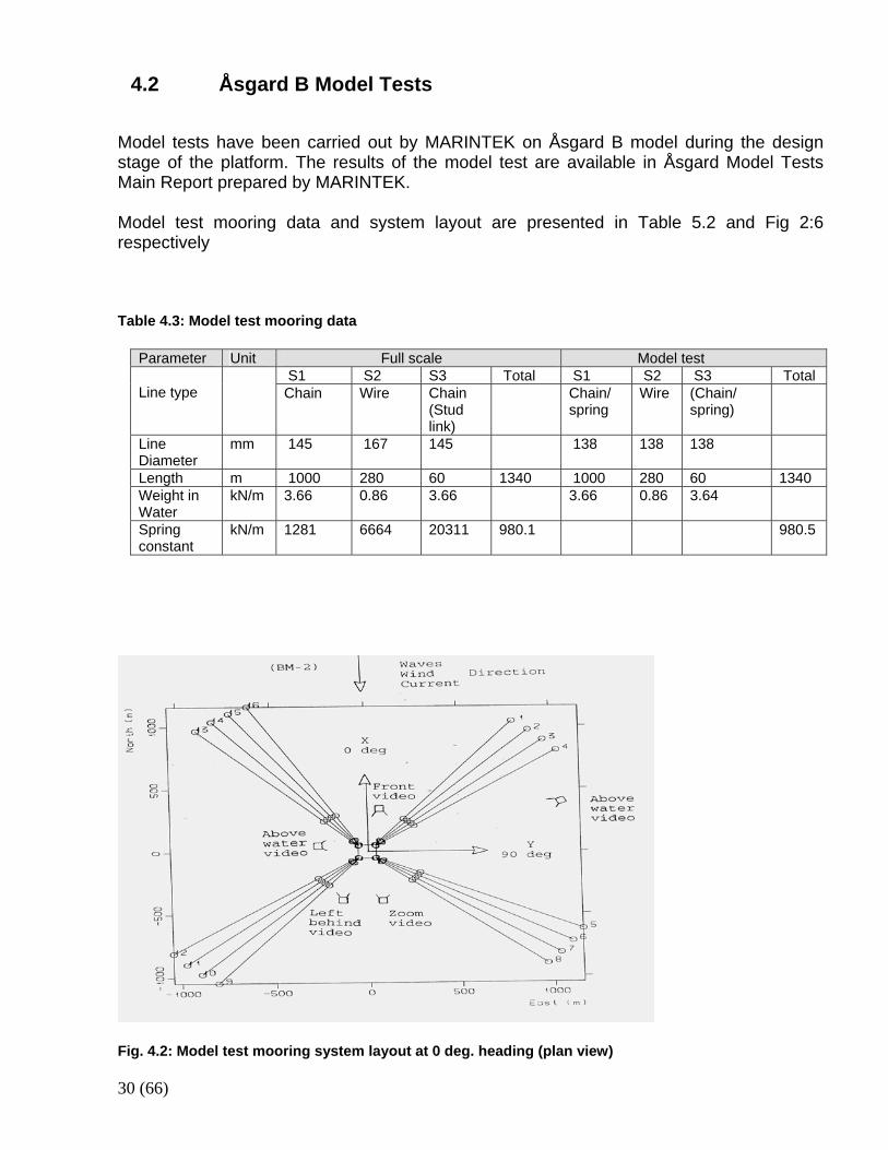
4.2 Åsgard B Model Tests

Model tests have been carried out by MARINTEK on Åsgard B model during the design stage of the platform. The results of the model test are available in Åsgard Model Tests Main Report prepared by MARINTEK. Model test mooring data and system layout are presented in Table 5.2 and Fig 2:6 respectively Table 4.3: Model test mooring data

Parameter Unit Full scale Model test S1 S2 S3 Total S1 S2 S3 Total

Line type

Chain Wire Chain (Stud link)

Chain/ spring

Wire (Chain/ spring)

Line Diameter

mm 145 167 145 138 138 138

Length m 1000 280 60 1340 1000 280 60 1340 Weight in Water

kN/m 3.66 0.86 3.66 3.66 0.86 3.64

Spring constant

kN/m 1281 6664 20311 980.1 980.5

Fig. 4.2: Model test mooring system layout at 0 deg. heading (plan view)

31 (66)

For the purpose of this work, we have selected two sea states (in three headings, 0, 45 and 90 deg.) that are close the selected reduced measured field data for ease of comparison of the results. These are shown in Table 4.4 Table 4.4: Model test selected sea states

Waves

Wind Current Tests no. Platform Heading Deg. Hs

m Tp s

Vw m/s

Vc m/s

201

0

10.7

11.0

33.5

0.80

301

90

10.7

11.0

33.5

0.80

Sea state 1

401

45

10.7

11.0

33.5

0.80

204

0

15.6

19.0

33.5

0.80

304

90

15.6

19.0

33.5

0.80

Sea state 2

404

45

15.6

19.0

33.5

0.80

32 (66)

5 CASH The software ‘Coupled Analysis Software for Hydrodynamics’ (CASH) was developed by GVA Consultant AB, Göteborg, Sweden. The general characteristics of the software are:

• The hydrodynamic analysis are performed in the time domain • All six degrees of freedom are included in the analysis

• The interaction between the vessel and the mooring and risers are included in the

time domain i.e. a fully coupled analysis is performed. The program performs a time domain simulation of a floating platform with mooring system fully coupled. It also requires motion and wave drift transfer functions from WADAM as input. CASH could run different wave and wind spectra such as JONSWAP, PM, NPD, etc. It solves the equation of motion by step by step integration using the Runge–Kutta method. The mooring line can be simulated quasi-statically or fully coupled. The line dynamics subroutines are taken from MODEX from Chalmers University of Technology, Göteborg, Sweden. The software is developed in Visual Fortran and can be run on a regular PC.

5.1 Advantages of the CASH Software

The advantages of using CASH software are several; a few examples are highlighted below:

• Dynamic interaction between semi and moorings • Current forces from lines and risers • Damping on lines and risers • Lines-soil interaction • Potential and viscous wave drift forces • Six degrees of freedom, 1st and 2nd order forces and motions • Uneven seabed can be simulated

(CASH User’s manual, version 2.9)

33 (66)

5.2 CASH VS Atlantis PQ-GVA 27000 CASH has been verified with Atlantis PQ-GVA 27000. (88,000 tonnes displacement semi-submersible platform with 12 chain–wire-chain type mooring lines and 8 SCR risers) in water depth of 2168 m. CASH was compared with the model test (truncated mooring lines at 520 m water depth), and calibration was done with the model test results. The numerical model analysis carried out with CASH showed motions that are close to the truncated model test results. Maximum line tensions are close or higher in the numerical model than obtained from the model tests for the most loaded lines. CASH numerical analysis was extended to full depth. The translational surge, sway and heave motions for the full-depth numerical system agrees with test results and with numerical results for the truncated system. Maximum predicted mooring line tensions for the full-depth system are lower than the allowed, so the mooring system used to plan the tank tests is considered adequate. (Model Test Truncation and Extrapolation to Full Depth, Atlantis PQ – GVA 27000 Report, 2003)

34 (66)

6 SOFTWARES A number of computer software was employed in the course of this thesis work. The most important ones are described below.

6.1 PreFix

Prefix is a 3D-Modeling tool, with an interface to finite element programs, in particular SESAM’s pre-processor Prefem. A model created in PreFIX may be exported to Prefem via an interface file. Prefem can then process this file and produce a SESAM Input Interface file, ready for analysis. PreFix is very good for geometric description and editing structural properties. It enables us to take advantage of Prefem’s strong sides, mesh generation and improve on others. One of the main advantages of PreFIX is the ability to work with library models. In this way, a structural detail may be modeled once, and stored. Later, you can retrieve this model, scale and position it into a new model. PreFIX‘s interface are similar to Windows’. (PreFix User’s manual, version 5.0, 1997-2001)

6.2 PREFEM

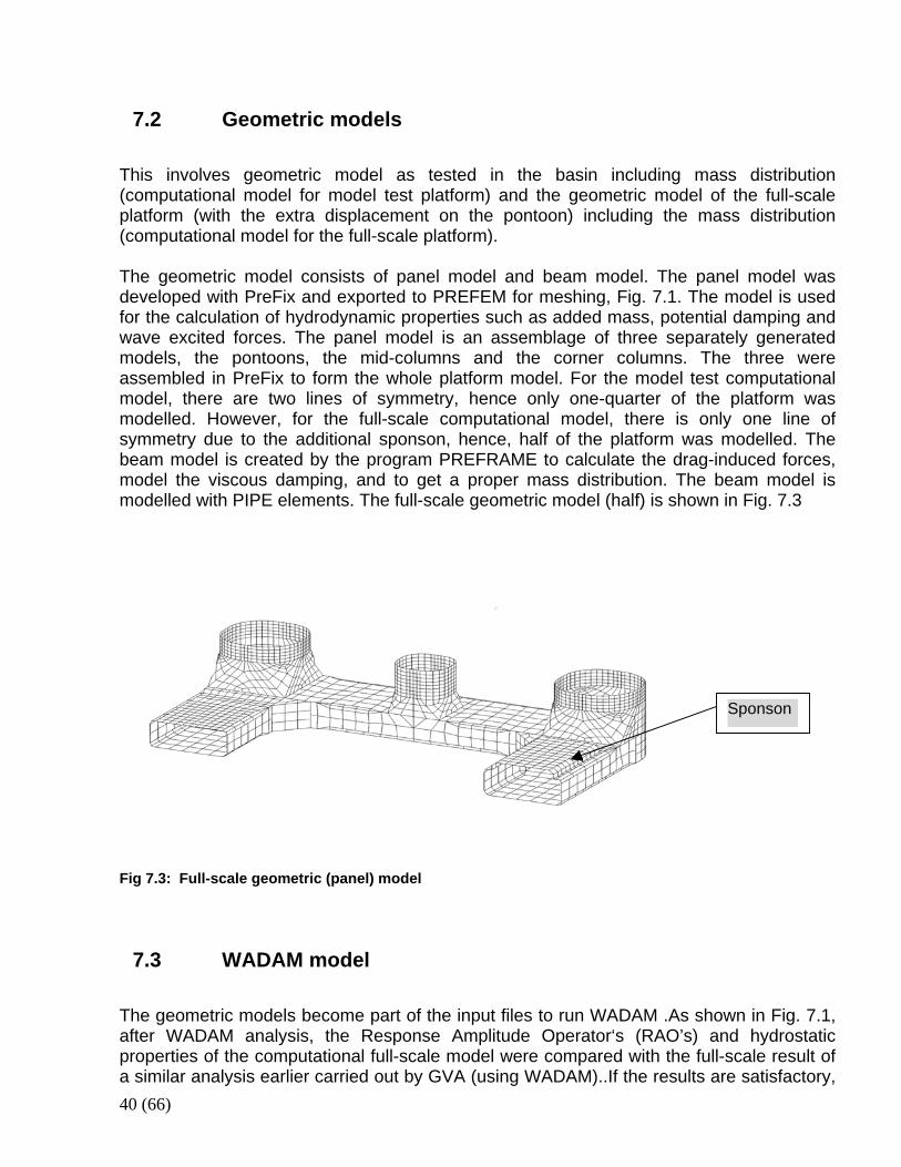
PREFEM is SESAM’s Preprocessor for general Finite Element (FE) Modeling. The models may be comprised of truss, beam, membrane, shell, and solid elements. More specialized elements like spring, damper and mass element, sandwich elements, contact elements and axis-symmetric elements are also available. Within the SESAM systems, the models are available for hydrodynamic as well as structural analysis. A model to be used for structural analysis is termed herein a FE model whereas a model to be used for hydrodynamic analysis is termed a panel model. A panel model may in certain cases be equal to a FE model (the one and only model is used for both structural and hydrodynamic analysis), but normally, it is somewhat different. Modeling a panel model will however, in principle be the same as modeling a FE model. PREFEM’s objectives are:

• To minimize the amount of data to be given by the user, thereby reducing the modeling time

• To ensure reliability of input data and • To enable establishing an adequate analysis model

The following main program features are provided to meet these objectives:

35 (66)

• Interactive input by two alternative modes -line input mode and

-graphic input mode • Graphic and printed feedback for verifying data • Extensive data generation function • A data management system allowing arbitrarily large models

(SESAM User’s manual, PREFEM, 1995)

6.3 WADAM

This program is used for hydrodynamic calculations of first order motion, RAOs, added mass, radiation damping and force coefficients (Quadratic Transfer Functions, QTFs) used as input to MIMOSA. WADAM (Wave Analysis by Diffraction and Morison Theory) is a general analysis program for calculation of wave-structure interaction for fixed and floating structures of arbitrary shape, e.g. semi-submersibles, tension-leg platforms, gravity-base structures and ship hulls. Some of the analysis capabilities in WADAM that will be further used for the mooring analysis are:

• Calculation of hydrostatic data and inertia properties • Calculation of global responses including

-first and second order wave excitation forces and moments -hydrodynamic added mass and damping -rigid body motions -steady drift forces and moments -sectional forces and moments -internal tank pressure

WADAM calculates loads using:

• Morison’s equation • First and second order 3D potential theory for large volume structures • Morison’s equation and potential theory when the structure comprises both slender

and large volume parts. The forces at the slender part may optionally be calculated using the diffracted wave kinematics calculated from the presence of the large volume part of the structure.

The WADAM results may be presented directly as complex transfer functions or converted to time domain results for a specified sequence of phase angles of the incident wave. For fixed structures, Morison’s equation may also be used with a time domain output option to calculate drag forces due to time independent current.

36 (66)

The 3D potential theory in WADAM is based directly on the WAMIT program developed by Massachusetts Institute of Technology, MIT. (SESAM User’s manual, WADAM, 1994)

6.4 MIMOSA

MIMOSA is an interactive computer program for static and dynamic analysis of moored vessels. It is capable of computing static and dynamic environmental loads, corresponding displacement and motion of the vessel and static and dynamic mooring tensions based on motion and wave drift transfer functions obtained from WADAM. The program is commonly used for purposes such as:

• Early concept and design studies • Parameter studies • Documentation of positioning systems at a certain location according to authority

guidelines and regulations. Static and quasi-static analysis including dynamic transient loading can be carried out for almost any type of system. Dynamic analysis is carried out in the frequency domain for both wave frequency and low-frequency motion and tension responses. MIMOSA is a computer program for analysis of mooring systems for moored vessels (semi, ships, etc).The program is up–to-date with respect to calculations required by the Norwegian Maritime Directorate (NMD) and the American Petroleum Institute (API) for approval of positioning systems, e.g. calculation of slow drift, line dynamics and transient motion. Frequency domain techniques to compute vessel motion and dynamic mooring tension are employed. Time domain transient analysis after line failure can also be performed by MIMOSA. MIMOSA covers:

- Static and dynamic environmental forces due to waves, wind and current - Wave induced motions - Slow drift motions - Static and dynamic mooring system analysis - Composite segments (e.g. chain and wire) mooring lines - Transient motions after line breakage - Non- Gaussian statistics - Yaw-Stability analysis of turret-moored ships - Static clearance (riser-mooring line) checks

(MIMOSA User’s documentation, Marintek, 1995)

37 (66)

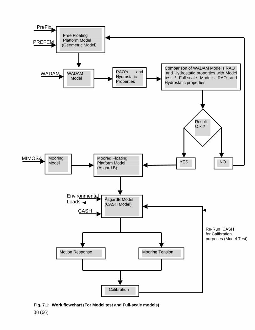
7 METHODOLOGY The detailed procedure adopted in the thesis work is presented graphically in Fig. 7.1. The thesis work has two components: i) Comparison of model test and fully coupled CASH analysis (calibration tests) ii) Comparison of measured field data and fully coupled CASH analysis

7.1 Coordinate systems There is the need to convert all the results (Model test and Field measurement) to CASH coordinate system for ease of comparison. CASH uses the right-hand-system with positive X towards platform aft, positive Z upwards and positive Y to portside. Fig. 7.2a compares Model test and CASH coordinate systems. The result is shown in Table 7.1. Field measurements and CASH however have the same coordinate system; this is shown in Fig. 7.2b. Table 7.1: Conversion of model test results to CASH coordinate system Degree of Freedom Model tests conversion sign Surge (-) Sway (+) Heave (-) Roll (-) Pitch (+) Yaw (-)

38 (66)

Fig. 7.1: Work flowchart (For Model test and Full-scale models)

Free Floating Platform Model (Geometric Model)

RAO’s and Hydrostatic Properties

NO Moored Floating Platform Model (Åsgard B)

Mooring Model

Calibration

Motion Response

ÅsgardB Model (CASH Model)

Mooring Tension

Comparison of WADAM Model’s RAO and Hydrostatic properties with Modeltest / Full-scale Model’s RAO and Hydrostatic properties

Result O.k ?

YES

PreFix

PREFEM

WADAM

MIMOSA

Environmental Loads

CASH

Re-Run CASH for Calibration purposes (Model Test)

WADAM Model

39 (66)

Roll

X, Surge (MODEL TEST)

X, Surge (CASH) Roll

Fig. 7.2a Model test and CASH coordinate system comparison Fig. 7.2b Field measurement and CASH coordinate system

Y, Sway (CASH, MODEL TEST)

Pitch

True North

Platform North

45

Aft Pontoon

Forward Pontoon

X (CASH, Field) Y (CASH, Field)

40 (66)

7.2 Geometric models This involves geometric model as tested in the basin including mass distribution (computational model for model test platform) and the geometric model of the full-scale platform (with the extra displacement on the pontoon) including the mass distribution (computational model for the full-scale platform). The geometric model consists of panel model and beam model. The panel model was developed with PreFix and exported to PREFEM for meshing, Fig. 7.1. The model is used for the calculation of hydrodynamic properties such as added mass, potential damping and wave excited forces. The panel model is an assemblage of three separately generated models, the pontoons, the mid-columns and the corner columns. The three were assembled in PreFix to form the whole platform model. For the model test computational model, there are two lines of symmetry, hence only one-quarter of the platform was modelled. However, for the full-scale computational model, there is only one line of symmetry due to the additional sponson, hence, half of the platform was modelled. The beam model is created by the program PREFRAME to calculate the drag-induced forces, model the viscous damping, and to get a proper mass distribution. The beam model is modelled with PIPE elements. The full-scale geometric model (half) is shown in Fig. 7.3

Fig 7.3: Full-scale geometric (panel) model

7.3 WADAM model The geometric models become part of the input files to run WADAM .As shown in Fig. 7.1, after WADAM analysis, the Response Amplitude Operator‘s (RAO’s) and hydrostatic properties of the computational full-scale model were compared with the full-scale result of a similar analysis earlier carried out by GVA (using WADAM)..If the results are satisfactory,

Sponson

41 (66)

then the model is considered good for the mooring analysis, otherwise, it is returned to PreFix / PREFEM for necessary amendments.

7.4 Mooring models We received the mooring model from STATOIL. Model test mooring system has been scaled statically. During the model test, the specified line lengths were modelled correctly in headings 0 deg. and 90 deg. In 45 deg. heading however, lines number 7, 8, 13 and 14 were shortened by 55 m , and lines number 9, 10, 11 and 12 by 170 m full-scale due to the available floor area in the basin. This resulted in two computational mooring models for the model test (one for 0, 90 deg. heading and another for 45 deg. heading). The computational model test mooring system was verified using MIMOSA (restoring forces). The restoring force results agreed well with the model test result .However, there was no pull-out test data to verify the computational full-scale mooring system received from STATOIL, we only assume possible error is negligible. To use the mooring model in CASH for dynamic analysis however, it has to be converted to CASH input version using a program called MODEX.

7.5 CASH model At this stage, we have a fully coupled computational models (model tests and full-scale), ready for CASH analysis. CASH combine the geometric and mooring models to create a floating moored system. Wind and current force coefficient from wind tunnel tests are included as part of CASH input files in addition to wave drift force coefficients form WADAM analysis. Environmental loads (wind, waves and current) are applied to the model for different loading conditions, sea states and headings (0, 45 and 90 degree respectively) and dynamic analysis is performed in CASH for the moored platform models. CASH output results include restoring forces, motions, mooring line tensions, etc. JONSWAP wave spectrum and NPD wind spectrum were used in the tests.

7.6 Calibrations Wind and current coefficients (from wind tunnel test) and wave drift coefficients (from WADAM analysis) are part of necessary inputs to CASH for dynamic analysis. These coefficients are scaled until they agree with the coefficients estimated from the model test this is to calibrate the computational model to the model test. Different test

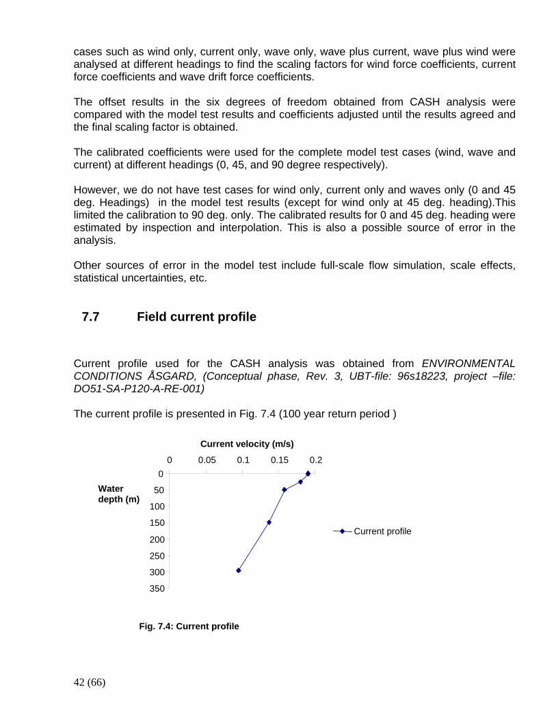
42 (66)

cases such as wind only, current only, wave only, wave plus current, wave plus wind were analysed at different headings to find the scaling factors for wind force coefficients, current force coefficients and wave drift force coefficients. The offset results in the six degrees of freedom obtained from CASH analysis were compared with the model test results and coefficients adjusted until the results agreed and the final scaling factor is obtained. The calibrated coefficients were used for the complete model test cases (wind, wave and current) at different headings (0, 45, and 90 degree respectively). However, we do not have test cases for wind only, current only and waves only (0 and 45 deg. Headings) in the model test results (except for wind only at 45 deg. heading).This limited the calibration to 90 deg. only. The calibrated results for 0 and 45 deg. heading were estimated by inspection and interpolation. This is also a possible source of error in the analysis. Other sources of error in the model test include full-scale flow simulation, scale effects, statistical uncertainties, etc.

7.7 Field current profile Current profile used for the CASH analysis was obtained from ENVIRONMENTAL CONDITIONS ÅSGARD, (Conceptual phase, Rev. 3, UBT-file: 96s18223, project –file: DO51-SA-P120-A-RE-001) The current profile is presented in Fig. 7.4 (100 year return period )

Fig. 7.4: Current profile

0

50

100

150

200

250

300

350

0 0.05 0.1 0.15 0.2

Current velocity (m/s)

Current profile

Water depth (m)

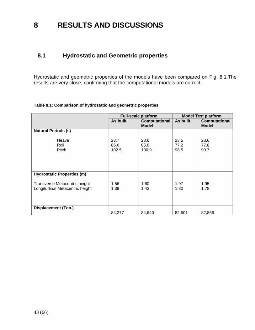
43 (66)

8 RESULTS AND DISCUSSIONS

8.1 Hydrostatic and Geometric properties Hydrostatic and geometric properties of the models have been compared on Fig. 8.1.The results are very close, confirming that the computational models are correct. Table 8.1: Comparison of hydrostatic and geometric properties

Full-scale platform Model Test platform As built Computational

Model As built Computational

Model Natural Periods (s) Heave Roll Pitch

23.7 86.6 102.5

23.6 85.8 100.9

23.5 77.2 98.5

23.6 77.8 90.7

Hydrostatic Properties (m) Transverse Metacentric height Longitudinal Metacentric height

1.56 1.39

1.60 1.43

1.97 1.80

1.95 1.78

Displacement (Ton.)

84,277

84,640

82,501

82,866

44 (66)

8.2 Response Amplitude Operators (RAOs ) The results of the Response Amplitude Operators (RAOs), is presented in Fig. 8.1 for the full scale models in five degrees of freedom. Comparison has been with an existing analysis carried out by GVA using full-scale model of Åsgard B platform. Close correlation is observed between the two sets of results in surge, sway, roll and pitch. In the heave mode however, the existing full-scale model has been restricted in motion amplitude to account for damping in the system.

Comparison of Response Amplitude Operator,RAO, for Surge Motion

00.20.40.60.8

11.21.4

0 20 40 60

Periods (s)

Computational full-scale modelExisting full-scale model

Comparison of Response Amplitude Operator,RAO, for Sway Motion

00.20.40.60.8

11.21.4

0 20 40 60

Period (s)

Computational full-scale model Existing full-scale model

Sway (m/m)

Surge (m/m)

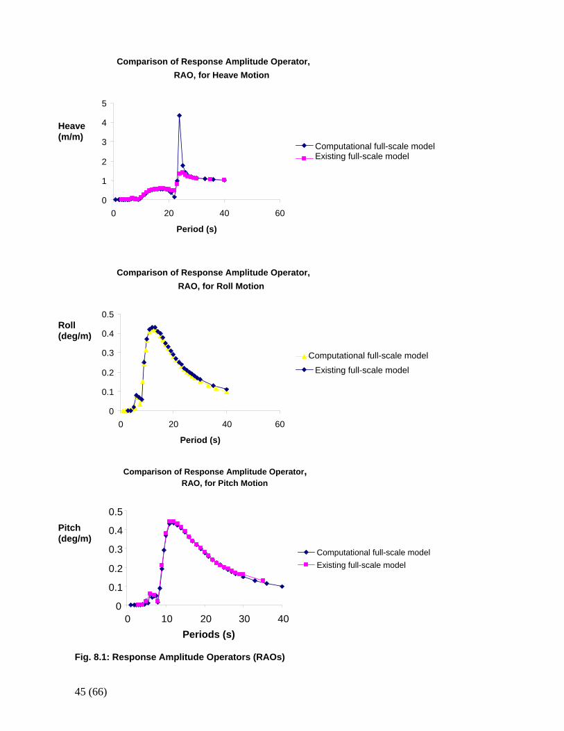
45 (66)

Fig. 8.1: Response Amplitude Operators (RAOs)

Comparison of Response Amplitude Operator, RAO, for Heave Motion

0

1

2

3

4

5

0 20 40 60

Period (s)

Computational full-scale modelExisting full-scale model

Comparison of Response Amplitude Operator, RAO, for Roll Motion

0

0.1

0.2

0.3

0.4

0.5

0 20 40 60

Period (s)

Computational full-scale model Existing full-scale model

Comparison of Response Amplitude Operator, RAO, for Pitch Motion

0

0.1

0.2

0.3

0.4

0.5

0 10 20 30 40Periods (s)

Computational full-scale model Existing full-scale model

Roll (deg/m)

Pitch (deg/m)

Heave (m/m)

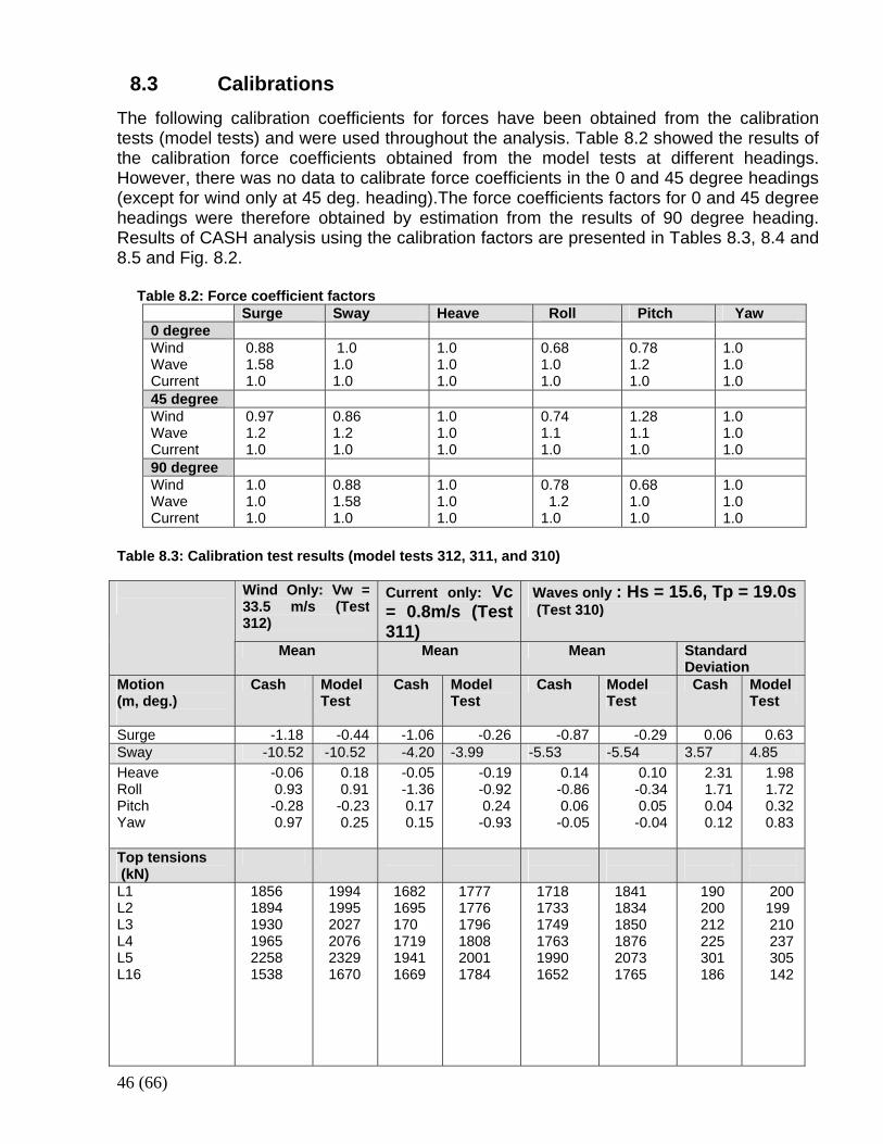
46 (66)

8.3 Calibrations The following calibration coefficients for forces have been obtained from the calibration tests (model tests) and were used throughout the analysis. Table 8.2 showed the results of the calibration force coefficients obtained from the model tests at different headings. However, there was no data to calibrate force coefficients in the 0 and 45 degree headings (except for wind only at 45 deg. heading).The force coefficients factors for 0 and 45 degree headings were therefore obtained by estimation from the results of 90 degree heading. Results of CASH analysis using the calibration factors are presented in Tables 8.3, 8.4 and 8.5 and Fig. 8.2. Table 8.2: Force coefficient factors

Surge Sway Heave Roll Pitch Yaw 0 degree Wind Wave Current

0.88 1.58 1.0

1.0 1.0 1.0

1.0 1.0 1.0

0.68 1.0 1.0

0.78 1.2 1.0

1.0 1.0 1.0

45 degree Wind Wave Current

0.97 1.2 1.0

0.86 1.2 1.0

1.0 1.0 1.0

0.74 1.1 1.0

1.28 1.1 1.0

1.0 1.0 1.0

90 degree Wind Wave Current

1.0 1.0 1.0

0.88 1.58 1.0

1.0 1.0 1.0

0.78 1.2 1.0

0.68 1.0 1.0

1.0 1.0 1.0

Table 8.3: Calibration test results (model tests 312, 311, and 310)

Wind Only: Vw = 33.5 m/s (Test 312)

Current only: Vc = 0.8m/s (Test 311)

Waves only : Hs = 15.6, Tp = 19.0s (Test 310)

Mean Mean Mean Standard Deviation

Motion (m, deg.)

Cash Model Test

Cash Model Test

Cash Model Test

Cash Model Test

Surge -1.18 -0.44 -1.06 -0.26 -0.87 -0.29 0.06 0.63 Sway -10.52 -10.52 -4.20 -3.99 -5.53 -5.54 3.57 4.85 Heave Roll Pitch Yaw

-0.06 0.93 -0.28 0.97

0.18 0.91 -0.23 0.25

-0.05 -1.36 0.17 0.15

-0.19 -0.92 0.24 -0.93

0.14 -0.86 0.06 -0.05

0.10 -0.34 0.05 -0.04

2.31 1.71 0.04 0.12

1.98 1.72 0.32 0.83

Top tensions (kN)

L1 L2 L3 L4 L5 L16

1856 1894 1930 1965 2258 1538

1994 1995 2027 2076 2329 1670

1682 1695 170 1719 1941 1669

1777 1776 1796 1808 2001 1784

1718 1733 1749 1763 1990 1652

1841 1834 1850 1876 2073 1765

190 200 212 225 301 186

200 199 210 237 305 142

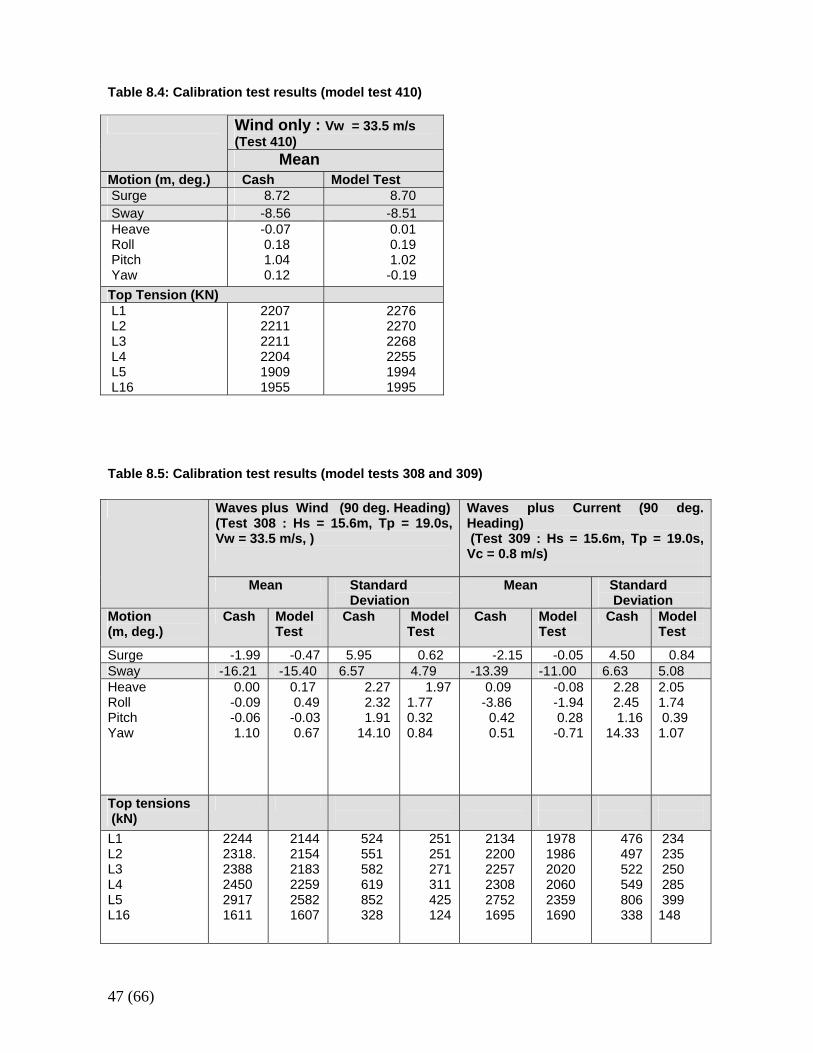
47 (66)

Table 8.4: Calibration test results (model test 410)

Wind only : Vw = 33.5 m/s (Test 410)

Mean Motion (m, deg.) Cash Model Test Surge 8.72 8.70 Sway -8.56 -8.51 Heave Roll Pitch Yaw

-0.07 0.18 1.04 0.12

0.01 0.19 1.02 -0.19

Top Tension (KN) L1 L2 L3 L4 L5 L16

2207 2211 2211 2204 1909 1955

2276 2270 2268 2255 1994 1995

Table 8.5: Calibration test results (model tests 308 and 309)

Waves plus Wind (90 deg. Heading) (Test 308 : Hs = 15.6m, Tp = 19.0s, Vw = 33.5 m/s, )

Waves plus Current (90 deg. Heading) (Test 309 : Hs = 15.6m, Tp = 19.0s, Vc = 0.8 m/s)

Mean Standard Deviation

Mean Standard Deviation

Motion (m, deg.)

Cash Model Test

Cash Model Test

Cash Model Test

Cash Model Test

Surge -1.99 -0.47 5.95 0.62 -2.15 -0.05 4.50 0.84 Sway -16.21 -15.40 6.57 4.79 -13.39 -11.00 6.63 5.08 Heave Roll Pitch Yaw

0.00 -0.09 -0.06 1.10

0.17 0.49 -0.03 0.67

2.27 2.32 1.91 14.10

1.97 1.77 0.32 0.84

0.09 -3.86 0.42 0.51

-0.08 -1.94 0.28 -0.71

2.28 2.45 1.16 14.33

2.05 1.74 0.39 1.07

Top tensions (kN)

L1 L2 L3 L4 L5 L16

2244 2318. 2388 2450 2917 1611

2144 2154 2183 2259 2582 1607

524 551 582 619 852 328

251 251 271 311 425 124

2134 2200 2257 2308 2752 1695

1978 1986 2020 2060 2359 1690

476 497 522 549 806 338

234 235 250 285 399 148

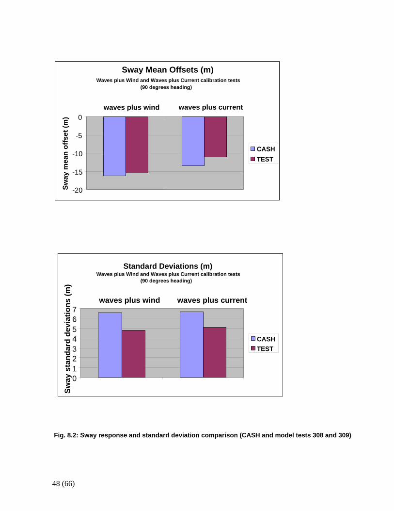
48 (66)

Fig. 8.2: Sway response and standard deviation comparison (CASH and model tests 308 and 309)

Sway Mean Offsets (m)Waves plus Wind and Waves plus Current calibration tests

(90 degrees heading)

-20

-15

-10

-5

0waves plus wind waves plus current

Sway

mea

n of

fset

(m)

CASHTEST

Standard Deviations (m)Waves plus Wind and Waves plus Current calibration tests

(90 degrees heading)

01234567

waves plus wind waves plus current

Sway

sta

ndar

d de

viat

ions

(m)

CASHTEST

49 (66)

8.4 CASH Vs Model Test: RESULTS AND DISCUSSIONS Results of CASH simulations and model tests for model tests 201, 301 and 401 are presented in Tables 8.6 and 8.7. The mean offsets and mean line tensions agree well with the model test results, indicating that the numerical simulation is good. The standard deviation of the sway motion in the three test cases (representing headings 0, 90 and 45 deg.) showed some disparity. This could be due to a number of reasons. It could be that the numerical model is unstable or weak in the sway direction. In the numerical analysis, riser stiffness and drag forces have not been included for lack of information (no information on riser stiffness and drag forces in the model tests report), whereas these were included in the model test, this makes the numerical model softer than the model test and also lead to reduced viscous damping in the system and hence higher mean offsets and standard deviations is expected in the numerical results. Current forces on the riser were also not accounted for, leading to reduced wave drift damping in the system. However, it is difficult to say this is responsible for the relatively high standard deviation observed in the sway direction for all the headings. There is also the possibility of errors in the any of the input files. We do not have information on current profile, we had to rely on current profile from ENVIRONMENTAL CONDITIONS ÅSGARD, (Conceptual, Rev. 3, UBT-file: 96s18223, project-file: DO51-SA-P120-A-RE-001) for the model test, this no doubt introduce some errors in the numerical wave drift damping computation. A constant current velocity of 0.8 m/s was used throughout the model test report. Generally speaking, damping correlation between the model test and numerical simulation is major source of error. The model test scaling has been done statically; this introduces differences in the drag coefficients between the model tests and the numerical test due to disparity in the value of Reynolds number (this was also stated in the model test report). Higher drag coefficient is therefore expected in the model test because of low Reynolds number in the test flow (model test flow is usually laminar). With the drag coefficient overestimated in the model test compared with the numerical test, this obviously affects viscous and mooring line damping computation results. From the foregoing, it is possible to say that the numerical model was under damped compared to the model test, therefore, more damping was added to the numerical computation in the sway direction. Different damping values of were tested until a close result is obtained in the sway standard deviations. With an added damping of 1E+07 Ns/m in the sway direction therefore, the standard deviations of the results improve greatly and this is shown in Tables 8.8 and 8.9 and plotted in Fig. 8.3. For test cases 204, 304 and 404 (with wave heights 15.6m) , the mean offsets and mean line tensions also agree with model tests, as shown in Tables 8.10 and 8.11.However, the high standard deviation shifted this time to yaw direction for all the headings and possible causes could be located in any of the sources of errors earlier discussed. Additional damping in yaw direction did not solve the problem; hence this is suggested as part of further work.

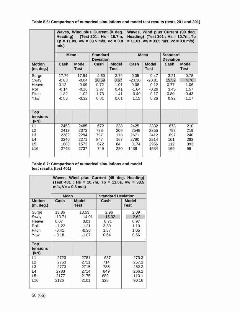
50 (66)

Table 8.6: Comparison of numerical simulations and model test results (tests 201 and 301)

Waves, Wind plus Current (0 deg. Heading) (Test 201 : Hs = 10.7m, Tp = 11.0s, Vw = 33.5 m/s, Vc = 0.8 m/s)

Waves, Wind plus Current (90 deg. Heading) (Test 301 : Hs = 10.7m, Tp = 11.0s, Vw = 33.5 m/s, Vc = 0.8 m/s)

Mean Standard Deviation

Mean Standard Deviation

Motion (m, deg.)

Cash Model Test

Cash Model Test

Cash Model Test

Cash Model Test

Surge Sway Heave Roll Pitch Yaw

17.79 -0.83 0.12 -0.14 -1.82 -0.83

17.94 -0.84 0.09 -0.16 -1.02 -0.32

4.60 20.59 0.72 3.97 1.73 0.81

3.72 0.67

1.01 0.41 1.41 0.61

0.35 -23.30 0.08 -1.64 -0.49 1.15

0.47 -20.81 0.12 -0.29 0.17 0.26

3.21 15.52 0.77 3.45 0.80 0.92

0.78 4.76 1.06 1.57 0.43 1.17

Top tensions (kN)

L1 L2 L3 L4 L5 L16

2453 2419 2382 2340 1688 2743

2485 2373 2294 2271 1573 2737

672 738 797 847 672 749

238 209 178 167 84 280

2425 2548 2671 2790 3174 1438

2332 2355 2412 2514 2956 1534

673 783 897 101 112 169

210 219 240 283 393 99

Table 8.7: Comparison of numerical simulations and model test results (test 401)

Waves, Wind plus Current (45 deg. Heading) (Test 401 : Hs = 10.7m, Tp = 11.0s, Vw = 33.5 m/s, Vc = 0.8 m/s)

Mean Standard Deviation Motion (m, deg.)

Cash Model Test

Cash Model Test

Surge Sway Heave Roll Pitch Yaw

13.85 -13.71 0.07 -1.23 -0.41 - 0.18

13.53 -14.01 0.01 -1.21 -0.36 -1.07

2.96 15.32 0.71 3.30 1.57 0.64

2.09 2.62

0.97 1.10 1.05 0.66

Top tensions (kN)

L1 L2 L3 L4 L5 L16

2723 2753 2773 2783 2177 2126

2781 2711 2715 2714 2175 2101

637 714 785 849 689 328

273.3 257.2 262.2 266.2 113.1 90.16

51 (66)

Table 8.8: Comparison of numerical simulations and model test results (tests 201 and 301; with Sway damping = 1E+ 07 Ns/m)

Table 8.9: Comparison of numerical simulations and model test results (test 401; with Sway damping = 1E+ 07 Ns/m )

Waves, Wind plus Current (45 deg. Heading) (Test 401 : Hs = 10.7m, Tp = 11.0s, Vw = 33.5 m/s, Vc = 0.8 m/s)

Mean Standard Deviation Motion (m, deg.)

Cash Model Test

Cash Model Test

Surge 14.01 13.53 2.78 2.09 Sway -13.74 -14.01 1.83 2.62 Heave Roll Pitch Yaw

0.08 -1.16 -0.45 - 0.15

0.01 -1.21 -0.36 -1.07

0.71 1.17 1.65 0.44

0.97 1.10 1.05 0.66

Top tensions (kN)

L1 L2 L3 L4 L5 L16

2633 2641 2640 2629 2034 2080

2781 2711 2715 2714 2175 2101

237 235 231 223 70 111

273 257 262 266 113 90

Waves, Wind plus Current (0 deg. Heading) (Test 201 : Hs = 10.7m, Tp = 11.0s, Vw = 33.5 m/s, Vc = 0.8 m/s)

Waves, Wind plus Current (90 deg. Heading) (Test 301 : Hs = 10.7m, Tp = 11.0s, Vw = 33.5 m/s, Vc = 0.8 m/s)

Mean Standard Deviation Mean Standard Deviation

Motion (m, deg.)

Cash Model Test

Cash Model Test

Cash Model Test

Cash Model Test

Surge 18.47 17.94 4.92 3.72 -0.10 0.47 1.21 0.78 -23.97 -20.81 6.12 4.76 Sway

Heave Roll Pitch Yaw

-1.53 0.13 -0.30 -2.02 -0.87

-0.84 0.09 -0.16 -1.02 -0.32

0.27 0.73 0.08 1.80 0.34

0.67 1.01 0.41 1.41 0.61

0.09 -1.68 -0.42 1.60

0.12 -0.29 0.17 0.26

0.77 2.07 0.32 0.52

1.06 1.57 0.43 1.17

Top tensions (kN)

L1 L2 L3 L4 L5 L16

2369 2309 2244 2177 1534 2613

2485 2373 2294 2271 1573 2737

261 237 211 185 99 313

238 209 178 167 84. 280

2320 2425 2528 2627 3037 1402

2332 2355 2412 2514 2956 1534

288 330 374 416 468 93

210 219 240 283 393 99.

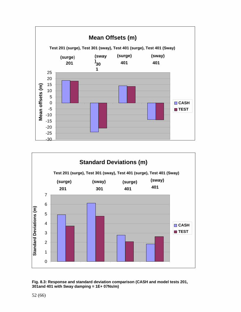
52 (66)

Fig. 8.3: Response and standard deviation comparison (CASH and model tests 201, 301and 401 with Sway damping = 1E+ 07Ns/m)

Mean Offsets (m) Test 201 (surge), Test 301 (sway), Test 401 (surge), Test 401 (Sway)

-30-25-20-15-10

-505

10152025

201

(surge)

301

(sway) 401

(surge)401

(sway)

Mea

n of

fset

s (m

)

CASHTEST

Standard Deviations (m) Test 201 (surge), Test 301 (sway), Test 401 (surge), Test 401 (Sway)

0

1

2

3

4

5

6

7

201

(surge)

301

(sway)

401

(surge)

401

(sway)

Stan

dard

Dev

iatio

ns (m

)

CASHTEST

53 (66)

Table 8.10: Comparison of numerical simulations and model test results (tests 204 and 304)

Waves, Wind plus Current (0 deg. Heading) (Test 204 : Hs = 15.6m, Tp = 19.0s, Vw = 33.5 m/s, Vc = 0.8 m/s)

Waves, Wind plus Current (90 deg. Heading) (Test 304 : Hs = 15.6m, Tp = 19.0s, Vw = 33.5 m/s, Vc = 0.8 m/s)

Mean Standard Deviation Mean Standard Deviation

Motion (m, deg.)

Cash Model Test

Cash Model Test

Cash Model Test

Cash Model Test

Surge Sway Heave Roll Pitch Yaw

18.94 -0.96 -0.01 -0.11 -3.19 -0.99

17.39 -0.15 0.09 -0.03 -0.10 -0.57

5.74 4.86 2.24 1.26 2.04 13.76

4.05 0.71 1.97 0.41 1.66 0.57

-1.33 -21.62 -0.02 -2.52 -0.12 1.49

-0.14 -19.86 0.07 -0.36 0.25 0.10

6.75 6.58 2.31 2.25 1.64 12.71

0.83 4.91 2.04 1.79 0.39 1.02

Top tensions (kN)

L1 L2 L3 L4 L5 L16

2663 2595 2518 2434 1686 2994

2437 2329 2245 2226 1543 2699

588 576 569 564 347 767

333 290 251 240 115 416

2432 2537 2637 2730 3252 1540

2297 2318 2360 2455 2873 1547

567 598 635 677 867 296

287 291 317 369 519 127

Table 8.11: Comparison of numerical simulations and model test results (test 404)

Waves, Wind plus Current (45 deg. Heading) (Test 404 : Hs = 15.6m, Tp = 19.0s, Vw = 33.5 m/s, Vc = 0.8 m/s)

Mean Standard Deviation Motion (m, deg.)

Cash Model Test

Cash Model Test

Surge Sway Heave Roll Pitch Yaw

15.23 14.42 -0.04 -1.94 -1.34 0.14

13.64 -13.65 0.02 -0.18 -0.04 -1.11

5.28 4.15 2.25 1.85 1.89 13.32

2.76 3.03 1.98 1.35 1.29 0.61

Top tensions (kN)

L1 L2 L3 L4 L5 L16

3071 3084 3080 3059 2280 2368

2782 2718 2714 2718 2155 2092

698 707 721 738 428 426

453 422 427 429 189 162

54 (66)

8.5 CASH Vs Reduced Measured Field Data

Results of CASH simulations and measured field data (sea state 2) are presented in Table 8.12. There is a fairly good correlation between the numerical simulation results and the reduced field data in terms of mean offset and standard deviations. However, close observation of the reduced field data in the surge and sway directions revealed an equal mean offset magnitude in the two directions, this implies the heading angle is probably 45 deg. (315 deg. in CASH). The numerical simulation was rerun with 315 deg. heading and a better result was obtained. This result is shown in Table 8.13 and Fig. 8.4. The results of CASH simulation and the reduced measured field data (sea state 5) are presented in table 8.14. CASH simulation results showed a good agreement with reduced field data in terms of mean offset and standard deviations. However, in the sway direction, CASH standard deviation was rather high. The numerical full scale model behaved similar to the numerical model test model, test 301, Table 8.6 (see results and discussions in section 8.4), possibly because they have close significant wave heights. Possible reason is the non-availability of measured field current in the field data. Åsgard B field location in the North Sea is known to have occasional high current speeds which we were not able to model correctly in the numerical analysis. This no doubt affects the wave drift damping. In addition, we could not include riser stiffness and drag forces in our modeling as details are not available, wave drift and viscous damping are therefore underestimated. In the numerical analysis, model test results have been used to calibrate the force coefficients used for the field data analysis, this is also a source of error as the full scale model is know to have higher displacement than the model test. There is the possibility of errors in the numerical model or input files. Measurement errors, wave directionality, wind and current heading changes are possible sources of errors in the measured field data. To compensate for the underestimated damping in the numerical model, additional damping 1E+07 Ns/m (obtained from the numerical model test results) was introduced in the sway direction the sway direction and the analysis performed again, the results showed a better correlation and is presented in Table 8.15 and Fig. 8.5. CASH simulation results for sea state 8 are shown in Table 8.16.The mean offsets agrees, there is however, standard deviation disparity in the yaw direction. The behaviour is also similar to the numerical model test 304, Table 8.10 (see results and discussions in section 8.4). Additional damping in yaw direction did not solve the problem; hence this is also suggested as part of further work. CASH calculated the mean line tensions at fairlead positions whereas the field data measured the average anchor tension; this explains the difference noticed in the line tension results.

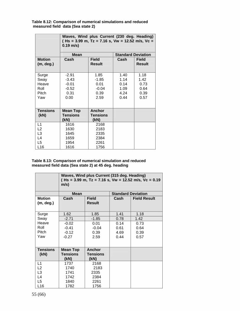
55 (66)

Table 8.12: Comparison of numerical simulations and reduced measured field data (Sea state 2)

Waves, Wind plus Current (230 deg. Heading) ( Hs = 3.99 m, Tz = 7.16 s, Vw = 12.52 m/s, Vc = 0.19 m/s)

Mean Standard Deviation Motion (m, deg.)

Cash Field Result

Cash Field Result

Surge Sway Heave Roll Pitch Yaw

-2.91 -3.43 -0.01 -0.52 0.31 0.00

1.85 -1.85 0.01 -0.04 0.39 2.59

1.40 1.14 0.14 1.09 4.24 0.44

1.18 1.42 0.73 0.64 0.39 0.57

Tensions (kN)

Mean Top Tensions (kN)

Anchor Tensions (kN)

L1 L2 L3 L4 L5 L16

1616 1630 1645 1659 1954 1616

2168 2183 2335 2384 2261 1756

Table 8.13: Comparison of numerical simulation and reduced measured field data (Sea state 2) at 45 deg. heading

Waves, Wind plus Current (315 deg. Heading) ( Hs = 3.99 m, Tz = 7.16 s, Vw = 12.52 m/s, Vc = 0.19 m/s)

Mean Standard Deviation Motion (m, deg.)

Cash Field Result

Cash Field Result

1.62 1.85 1.41 1.18 -2.71 -1.85 0.78 1.42

Surge Sway Heave Roll Pitch Yaw

-0.02 -0.41 -0.12 -0.27

0.01 -0.04 0.39 2.59

0.14 0.61 4.69 0.44

0.73 0.64 0.39 0.57

Tensions (kN)

Mean Top Tensions (kN)

Anchor Tensions (kN)

L1 L2 L3 L4 L5 L16

1737 1740 1741 1742 1840 1782

2168 2183 2335 2384 2261 1756

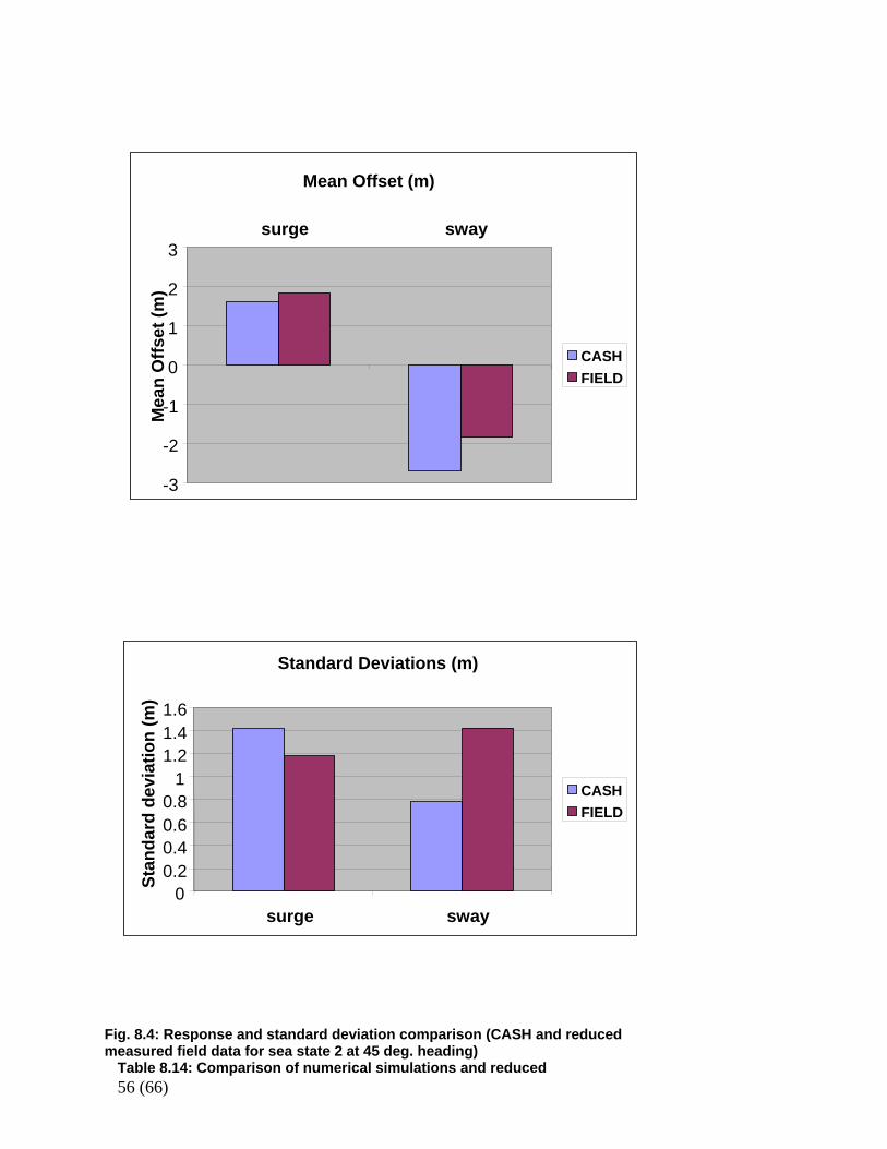
56 (66)

Fig. 8.4: Response and standard deviation comparison (CASH and reduced measured field data for sea state 2 at 45 deg. heading)

Table 8.14: Comparison of numerical simulations and reduced

Mean Offset (m)

-3

-2

-1

0

1

2

3surge sway

Mea

n O

ffset

(m)

CASHFIELD

Standard Deviations (m)

00.20.40.60.8

11.21.41.6

surge sway

Stan

dard

dev

iatio

n (m

)

CASHFIELD

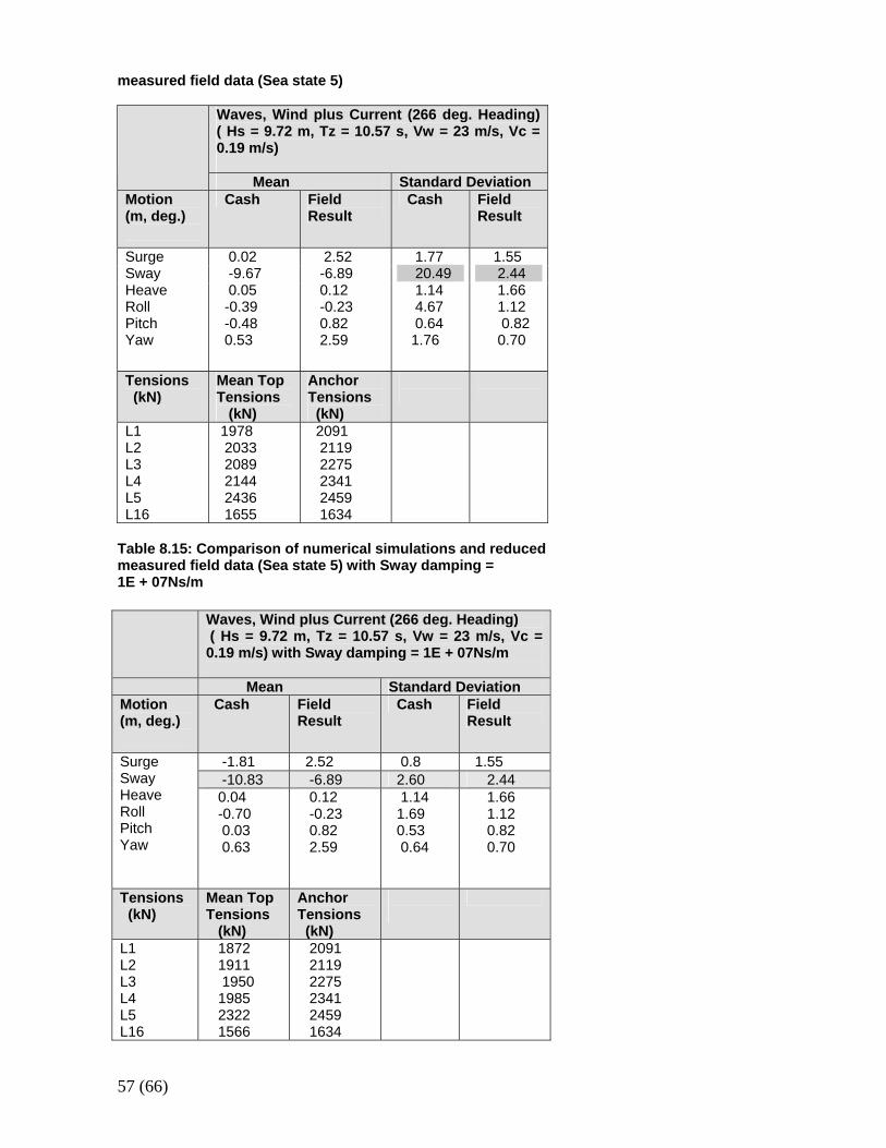
57 (66)

measured field data (Sea state 5)

Waves, Wind plus Current (266 deg. Heading) ( Hs = 9.72 m, Tz = 10.57 s, Vw = 23 m/s, Vc = 0.19 m/s)

Mean Standard Deviation Motion (m, deg.)

Cash Field Result

Cash Field Result

Surge Sway Heave Roll Pitch Yaw

0.02 -9.67 0.05 -0.39 -0.48 0.53

2.52 -6.89 0.12 -0.23 0.82 2.59

1.77 20.49 1.14 4.67 0.64 1.76

1.55 2.44 1.66 1.12 0.82 0.70

Tensions (kN)

Mean Top Tensions (kN)

Anchor Tensions (kN)

L1 L2 L3 L4 L5 L16

1978 2033 2089 2144 2436 1655

2091 2119 2275 2341 2459 1634

Table 8.15: Comparison of numerical simulations and reduced measured field data (Sea state 5) with Sway damping = 1E + 07Ns/m

Waves, Wind plus Current (266 deg. Heading) ( Hs = 9.72 m, Tz = 10.57 s, Vw = 23 m/s, Vc = 0.19 m/s) with Sway damping = 1E + 07Ns/m

Mean Standard Deviation Motion (m, deg.)

Cash Field Result

Cash Field Result

-1.81 2.52 0.8 1.55 -10.83 -6.89 2.60 2.44

Surge Sway Heave Roll Pitch Yaw

0.04 -0.70 0.03 0.63

0.12 -0.23 0.82 2.59

1.14 1.69 0.53 0.64

1.66 1.12 0.82 0.70

Tensions (kN)

Mean Top Tensions (kN)

Anchor Tensions (kN)

L1 L2 L3 L4 L5 L16

1872 1911 1950 1985 2322 1566

2091 2119 2275 2341 2459 1634

58 (66)

Fig. 8.5: Response and standard deviation comparison (CASH and reduced measured field data for sea state 5) with Sway damping = 1E+ 07Ns/m Table 8.16: Comparison of numerical simulation and reduced

Sway Mean Offset (m)

-12

-10

-8

-6

-4

-2

0Sway

Sway

mea

n of

fset

(m)

CASHFIELD

Standard Deviations (m)

2.35

2.4

2.45

2.5

2.55

2.6

2.65Sway

Sway

Sta

ndar

d D

evia

tion

(m)

CASHFIELD

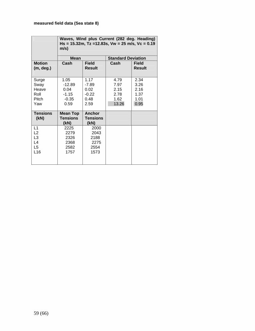
59 (66)

measured field data (Sea state 8)

Waves, Wind plus Current (282 deg. Heading) Hs = 15.32m, Tz =12.83s, Vw = 25 m/s, Vc = 0.19 m/s)

Mean Standard Deviation Motion (m, deg.)

Cash Field Result

Cash Field Result

Surge Sway Heave Roll Pitch Yaw

1.05 -12.89 0.04 -1.15 -0.35 0.59

1.17 -7.89 0.02 -0.22 0.48 2.59

4.79 7.97 2.15 2.78 1.62 13.26

2.34 3.26 2.16 1.37 1.01 0.95

Tensions (kN)

Mean Top Tensions (kN)

Anchor Tensions (kN)

L1 L2 L3 L4 L5 L16

2225 2279 2326 2368 2582 1757

2000 2043 2188 2275 2554 1573

60 (66)

9 CONCLUSIONS AND FURTHER WORK

This work has been carried out to compare the time domain numerical simulations as carried out by CASH with model test results and measure field data for Åsgard B platform. As indicated by the various results presented in this report, CASH has proved to be a good time domain numerical analysis tool. CASH results agreed well for the model tests and reduced measure field data in terms of mean offset and tension. The standard deviation results were significantly improved with increased damping in the system for waves of up to approximately 10 m significant wave height. Further work is suggested to determine:

1. The contribution of different damping components (wave drift, viscous and mooring

line) in the in the overall damping of the system .This is with a view to obtaining a better results from the numerical simulation.

2. Damping distribution in the different degrees of freedom need to be looked into.

3. Other possible causes of this disparity in standard deviation should be investigated

61 (66)

10 REFERENCES

A. Almar – Naess (1985) FATIGUE HANDBOOK, Tapir, Norges tekniske högskole API RP 2SK (1997) Recommended Practice for Design and Analysis of Stationkeeping Systems for Floating Structures ÅSGARD B MODEL TESTS (Main Report) MT51 F97-0198 Kvaerner Engineering a.s Marintek, Trondheim, Norway, 1997 report. ÅSGARD B SEMI-SUBMERSIBLE WIND TUNNEL TESTING Kvaerner Engineering a.s KVAERNER FLOATER DEVELOPMENT PROJECT.BMT Fluid Mechanics Limited, 1997 Atlantis PQ-GVA 27000 Report, Model Test Truncation and Extrapolation to Full Depth, doc. No. 1440-50-HY-RP-050-0091 Chakrabarti, S.K (1987) Hydrodynamics of Offshore Structures, Computational Mechanics Publications, Southampton, Boston Chakrabarti S.K (1990) Nonlinear methods in Offshore Engineering. Elsevier Science Publishers. Chakrabarti, S.K. (2002) The Theory and Practice Of Hydrodynamics and Vibration. World Scientific Publishing, New Jersey DET NORSKE VERITAS (DNV) SESAM USER’S MANUAL, PREFEM, 1994 DET NORSKE VERITAS (DNV) SESAM USER’S MANUAL, WADAM, 1994 Faltinsen O.M (1993) Sea Loads on Ships and Offshore Structures. Cambridge University Press GVA-C User’s Manual for CASH version 2.9. , 29 Nov. 2002. GVA Consultants AB, Göteborg, Sweden Liu.Y. and Aneljung. D. (2003) Fully–Coupled Analysis in Deepwater Model Tests; Deep Offshore Technology 2003, International Conference and Exhibition, Parc Chanot, Marseille, France Liu.Y. (1997) Dynamic analysis of mooring cables and their damping effect on the low-frequency motion of floating platforms. Report Series A: 28, Department of Hydraulics, Chalmers Univeristy of Technology, Göteborg, Sweden. MIMOSA User’s documentation. Marintek report.Marintek, Trondheim, Norway, August 1995 PreFix User’s manual ver. 5.0, Odd Solheim Solutions (1997-2001)

62 (66)

Randall (1997) Elements of Ocean Engineering, The Society of Naval Architects and Marine Engineers, New Jersey Rosen.B., and Brännström.O. (1999) Time –domain analysis of moored floating platforms, Department of Hydraulics, Chalmers Univeristy of Technology, Göteborg, Sweden STATOIL: Environmental Cnditions Åsgard. Conceptual phase, Revision 3 UBT-file: 96s18223, project –file: D051-SA-P120-A-RE-001 .

63 (66)

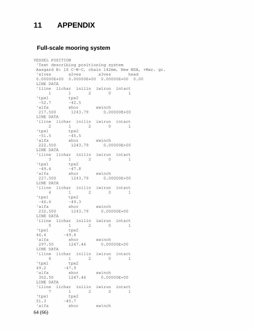
64 (66)

11 APPENDIX Full-scale mooring system VESSEL POSITION 'Text describing positioning system Aasgard B: 16 C-W-C, chain 142mm, New MSA, +Mar. gr. 'x1ves x2ves x3ves head 0.00000E+00 0.00000E+00 0.00000E+00 0.00 LINE DATA 'iline lichar inilin iwirun intact 1 1 2 0 1 'tpx1 tpx2 -52.7 -42.5 'alfa xhor xwinch 217.500 1243.79 0.00000E+00 LINE DATA 'iline lichar inilin iwirun intact 2 1 2 0 1 'tpx1 tpx2 -51.5 -45.5 'alfa xhor xwinch 222.500 1243.79 0.00000E+00 LINE DATA 'iline lichar inilin iwirun intact 3 1 2 0 1 'tpx1 tpx2 -49.4 -47.8 'alfa xhor xwinch 227.500 1243.79 0.00000E+00 LINE DATA 'iline lichar inilin iwirun intact 4 1 2 0 1 'tpx1 tpx2 -46.6 -49.3 'alfa xhor xwinch 232.500 1243.79 0.00000E+00 LINE DATA 'iline lichar inilin iwirun intact 5 1 2 0 1 'tpx1 tpx2 46.4 -49.4 'alfa xhor xwinch 297.50 1247.46 0.00000E+00 LINE DATA 'iline lichar inilin iwirun intact 6 1 2 0 1 'tpx1 tpx2 49.2 -47.9 'alfa xhor xwinch 302.50 1247.46 0.00000E+00 LINE DATA 'iline lichar inilin iwirun intact 7 1 2 0 1 'tpx1 tpx2 51.3 -45.7 'alfa xhor xwinch

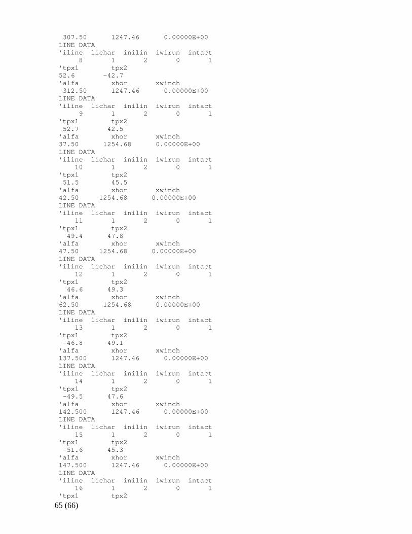
65 (66)

307.50 1247.46 0.00000E+00 LINE DATA 'iline lichar inilin iwirun intact 8 1 2 0 1 'tpx1 tpx2 52.6 -42.7 'alfa xhor xwinch 312.50 1247.46 0.00000E+00 LINE DATA 'iline lichar inilin iwirun intact 9 1 2 0 1 'tpx1 tpx2 52.7 42.5 'alfa xhor xwinch 37.50 1254.68 0.00000E+00 LINE DATA 'iline lichar inilin iwirun intact 10 1 2 0 1 'tpx1 tpx2 51.5 45.5 'alfa xhor xwinch 42.50 1254.68 0.00000E+00 LINE DATA 'iline lichar inilin iwirun intact 11 1 2 0 1 'tpx1 tpx2 49.4 47.8 'alfa xhor xwinch 47.50 1254.68 0.00000E+00 LINE DATA 'iline lichar inilin iwirun intact 12 1 2 0 1 'tpx1 tpx2 46.6 49.3 'alfa xhor xwinch 62.50 1254.68 0.00000E+00 LINE DATA 'iline lichar inilin iwirun intact 13 1 2 0 1 'tpx1 tpx2 -46.8 49.1 'alfa xhor xwinch 137.500 1247.46 0.00000E+00 LINE DATA 'iline lichar inilin iwirun intact 14 1 2 0 1 'tpx1 tpx2 -49.5 47.6 'alfa xhor xwinch 142.500 1247.46 0.00000E+00 LINE DATA 'iline lichar inilin iwirun intact 15 1 2 0 1 'tpx1 tpx2 -51.6 45.3 'alfa xhor xwinch 147.500 1247.46 0.00000E+00 LINE DATA 'iline lichar inilin iwirun intact 16 1 2 0 1 'tpx1 tpx2

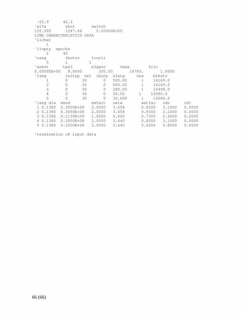
66 (66)

-52.9 42.3 'alfa xhor xwinch 152.500 1247.46 0.00000E+00 LINE CHARACTERISTICS DATA 'lichar 1 'linpty npocha 2 40 'nseg ibotco icurli 5 1 1 'anbot tpx3 x3ganc tmax fric 0.00000E+00 8.8000 300.00 16785. 1.0000 'iseg ieltyp nel ibuoy sleng nea brkstr 1 0 30 0 500.00 1 16169.0 2 0 30 0 500.00 1 16169.0 3 0 30 0 280.00 1 16488.0 4 0 30 0 30.00 1 16580.0 5 0 30 0 30.000 1 16580.0 'iseg dia emod emfact uwiw watfac cdn cdl 1 0.1380 0.3000E+08 2.0000 3.658 0.8300 3.1000 0.0000 2 0.1380 0.3000E+08 2.0000 3.658 0.8300 3.1000 0.0000 3 0.1380 0.1130E+09 1.0000 0.860 0.7300 2.6000 0.0000 4 0.1380 0.3000E+08 2.0000 3.640 0.8300 3.1000 0.0000 5 0.1380 0.3000E+08 2.0000 3.640 0.6500 5.8000 0.0000 'termination of input data