comparison of shell-and-tube with plate heat exchangers ... · in this paper, the con guration of...

Comparison of shell-and-tube with plate heat exchangers for the use inlow-temperature organic Rankine cyclesI

Daniel Walravena,c, Ben Laenenb,c, William D’haeseleera,c,∗

aUniversity of Leuven (KU Leuven) Energy Institute - TME branch (Applied Mechanics and Energy Conversion),Celestijnenlaan 300A box 2421, B-3001 Leuven, Belgium

bFlemish Institute for Technological Research (VITO), Boeretang 200, B-2400 Mol, BelgiumcEnergyVille (joint venture of VITO and KU Leuven), Dennenstraat 7, B-3600 Genk, Belgium

Abstract

Organic Rankine cycles (ORCs) can be used for electricity production from low-temperature heat sources.These ORCs are often designed based on experience, but this experience will not always lead to the mostoptimal configuration. The ultimate goal is to design ORCs by performing a system optimization. In suchan optimization, the configuration of the components and the cycle parameters (temperatures, pressures,mass flow rate) are optimized together to obtain the optimal configuration of power plant and components.In this paper, the configuration of plate heat exchangers or shell-and-tube heat exchangers is optimizedtogether with the cycle configuration. In this way every heat exchanger has the optimum allocation of heatexchanger surface, pressure drop and pinch-point-temperature difference for the given boundary conditions.ORCs with plate heat exchangers perform mostly better than ORCs with shell-and-tube heat exchangers,but one disadvantage of plate heat exchangers is that the geometry of both sides is the same, which canresult in an inefficient heat exchanger. It is also shown that especially the cooling-fluid inlet temperatureand mass flow have a strong influence on the performance of the power plant.

Keywords: ORC, Shell-and-tube heat exchanger, Plate heat exchanger, System optimization

1. Introduction

Low-temperature geothermal heat sources are widely available [1], but the electricity production efficiency islow due to the low temperature. Many authors have tried to maximize the electricity production efficiency oforganic Rankine cycles (ORCs) [2–4] by optimizing the cycle parameters (pressures, temperatures and massflow rates). To perform such an optimization, simplifying assumptions are made about the components, butthese assumptions can have a strong influence on the performance and the cost of the ORC.

As already explained in our previous work [5], this issue is already touched upon in the literature. Mad-hawa Hettiarachchi et al. [6] minimized the ratio of the total heat-exchanger surface and the net electricalpower produced by the cycle, for a fixed heat-exchanger configuration. Quoilin et al. [7] developed an ORCmodel and plate heat exchanger models based on their experimental set-up, while neglecting the pressuredrop in the heat exchangers. They used these models to predict the performance of their set-up in differentworking conditions. Shengjun et al. [8] maximized the performance of ORCs with shell-and-tube heat ex-changers, while keeping the configuration of the heat exchangers fixed. Domingues et al. [9] optimized ORCswith shell-and-tube heat exchangers for vehicle exhaust waste heat recovery and investigated the effect of the

IPublished version: http://dx.doi.org/10.1016/j.enconman.2014.07.019∗Corresponding author. Tel.: +32 16 32 25 11; fax: +32 16 32 29 85.Email addresses: [email protected] (Daniel Walraven), [email protected] (Ben Laenen),

[email protected] (William D’haeseleer)

Preprint submitted to Energy Conversion and Management July 9, 2014

number of tubes in the shell-and-tube heat exchangers on the performance of the ORC. Another approachwas followed by Franco and Villani [10]. They divided the ORC in a system level and a component level.In a first step, the system level was optimized, followed by the optimization of the configuration of thecomponents for the obtained optimal system configuration. An iteration between the optimization of bothlevels was needed to come to the final solution.

To obtain the global optimum configuration of the ORC, the system and the components should be op-timized together so that the configuration of the components is optimal for the use in the cycle and so thatthe components are adjusted to each other. To perform such a system optimization, realistic models, whichdescribe the performance of the components depending on geometric parameters, are needed.

In this paper models for heat exchangers are implemented and included in the system optimization. Bothshell-and-tube heat exchangers and plate heat exchangers are discussed. In previous research [5] we haveperformed a detailed investigation of shell-and-tube heat exchangers integrated in ORCs. The shell-and-tubeheat exchangers are modeled with the Bell-Delaware method [11, 12], which is a mature model and can beused for single-phase flow, condensing and evaporation.

The purpose of our research reported in this paper is to integrate plate heat exchangers in ORCs andto compare the result to that obtained with shell-and-tube heat exchangers. Martin [13] developed a modelfor plate heat exchangers with single-phase flow. This model is based on physical reasoning and many ex-perimental data are used. Such generally applicable models do not exist for two-phase plate heat exchangersused as evaporators or condensers, although much research has been performed on the topic [14–20]. Theauthors of those references propose correlations for heat-transfer coefficient and pressure drop based on ownexperiments and these correlations are therefore only valid for the investigated cases. We shall utilize thecorrelations of Han et al. [16] and Han et al. [17] for evaporation and condensation in plate heat exchangers,respectively. These papers correlate the performance of plate heat exchangers to many geometrical param-eters.

This paper extends the work performed in Walraven et al. [5], in which ORCs with shell-and-tube heatexchangers are optimized for a reference case. The conclusion from that work is that it is optimal to use the30◦ and 60◦ tube configurations in single and two-phase heat exchangers, respectively. In this paper, modelsfor plate heat exchangers are added and ORCs with plate heat exchangers are compared to ORCs withshell-and-tube heat exchangers (with the optimal tube configuration). The influence of the heat-source-inlettemperature, heat-source-outlet temperature, total heat exchanger surface, cooling-fluid inlet temperatureand the cooling fluid mass flow rate on the performance of the power plant are also investigated. Thecomparison between ORCs with the two different types of heat exchangers is performed in a wide range ofparameters and for many fluids.

2. Organic Rankine cycle

Different types of ORCs exist and are simulated in this paper. The investigated cycles can be of the simpleor recuperated type, be subcritical or transcritical and can have one or two pressure levels. Two examplesare given in figure 1, in which the scheme of a single-pressure, recuperated ORC and a double-pressure, sim-ple ORC are shown. All the possible heat exchangers (economizer, evaporator, superheater, desuperheater,condenser and recuperator) are shown in the figure, but are not always necessary.

In all configurations it is assumed that state 1 is saturated liquid and that the isentropic efficiencies ofthe pump and turbine are 80 and 85%, respectively. More information of the modeling can be found in pre-vious work [4, 5]. Instead of assuming a fixed pinch point temperature difference and ideal heat exchangers,models are used to calculate the heat transfer coefficients and pressure drops in each heat exchanger.

2

Cooling outCooling in

Heat source inHeat source out

1

2

3

4 56

7

8

9

(a) Single-pressure

Cooling outCooling in

Heat source in

Hea

tso

urc

eou

t

1 9 7

2 4b 5b 6b

1a2a 4a 5a 6a

(b) Double-pressure

Figure 1: Scheme of a single-pressure, recuperated (a) and double-pressure, simple (b) ORC.

3. Shell-and-tube heat exchanger

The shell-and-tube heat exchanger type has already been studied in Walraven et al. [5]. Here we now recallsome elements to support the later analysis with plate heat exchangers. TEMA E type heat exchangerswith a single shell pass and with the inlet and the outlet at the opposite ends of the shell are modeled. Theworking fluid always flows on the shell side, so models for the pressure drop and heat-transfer coefficient insingle-phase flow, evaporation and condensation in a TEMA E shell are needed. The tube-side fluid (theheat source) will always be single phase.

Lb,cLb,i

Lb,o

Ds

lc

pt

Dotl

θb

θctl

do

Dctl

Figure 2: Shell-and-tube geometrical characteristics. Figure adapted from Shah and Sekulic [12]. See also Walraven et al. [5].

Figure 2 recalls the basic geometrical characteristics of a shell-and-tube heat exchanger. These are theshell outside diameter Ds, the outside diameter of a tube do, the pitch between the tubes pt, the baffle cutlength lc and the baffle spacing at the inlet Lb,i, outlet Lb,o and the center Lb,c. More detailed informationabout the shell-and-tube model used in this paper can be found in Walraven et al. [5].

3

4. Plate Heat Exchanger

Plate heat exchangers can have many different types of corrugations [12], but in this paper only heatexchangers with chevron, also known as herringbone, corrugations are used. This type of corrugation iscommonly used and models which describe the pressure drop and heat transfer depending on the heatexchanger geometry are available [13, 16, 17]. The number of passes on both sides of the heat exchangersare assumed to be equal in this paper.

4.1. GeometryFigure 3 shows the geometrical parameters of a chevron plate. The corrugations are determined by thecorrugation amplitude a, the corrugation width Λ and the angle of the corrugations β. The width of a plateW , the length of a plate between ports Lp and the length of a plate for heat transfer Lh are also indicated.

Figure 3: Geometrical parameters of a chevron plate. Figure from Shah and Sekulic [12].

The hydraulic diameter is defined as:

Dh =4a

Φ, (1)

where Φ = 16

(1 +√

1 +X2 + 4√

1 +X2/2)

is the area-enlargement factor and X = 2πaΛ the dimensionless

corrugation parameter.

4.2. Heat-transfer and pressure-drop correlationsThe correlations of Martin [13] are used to predict the heat-transfer coefficient and the pressure drop in thesingle-phase heat exchangers. For the evaporator and the condenser, the correlations of Han et al. [16] andHan et al. [17] are used, respectively. An overview of these correlations is given in Appendix A.

4.3. Implementation of the modelsTo account for non-uniform fluid properties, each heat exchanger is divided into five parts with an equalheat load1. This number is chosen, because it leads to a reasonable accuracy and calculation time. For eachheat exchanger, the configuration (a, Λ, β and W Np), the inlet states at one side of the heat exchanger anda necessary outlet condition (e.g. the working fluid has to be saturated vapor at the end of the evaporator)are needed. The variables W and Np are combined to one variable, because only their product appears inthe equations. With these data, the total heat that has to be transferred in the case of no pressure drop2

can be calculated. In each of the five parts one fifth of this total heat will be exchanged. With the equationsabove, the heat-transfer coefficient and the pressure drop in the first part can be calculated. In this way,the state after the first part, the necessary heat-transfer surface and the fictive plate length of the first partcan be calculated. This procedure is repeated for the other parts, except in the last part for which the heatto be transferred is corrected for the pressure drop in the previous parts.

1These parts generally do not have the same physical size.2This is a starting value. The effect of the pressure drop on the heat load is taken into account in the last part of the heat

exchanger.

4

5. Optimization

5.1. Objective function

The goal of the optimization is to find a system configuration which maximizes the mechanical work outputfor a given heat source. This is the same as maximizing the exergetic plant efficiency [4], defined as:

ηplantex =Wnet

msourceesourcein

(2)

with Wnet the net mechanical-power production of the power plant, msource the mass flow of the source andesourcein the flow exergy of the source.

5.2. Optimization variables and constraints

The optimization variables which determine the cycle configuration in a single-pressure, simple cycle are thetemperature and saturation temperature at the pressure before the turbine T6 and T sat(p6), the mass flowof working fluid mwf and the temperature after the condenser T1. For a recuperated cycle, the tempera-ture difference between states 2 and 8 is added as an optimization variable. For a double-pressure cycle, T b6 ,T sat(pb6) and mb

wf are added as optimization variables. More information can be found in Walraven et al. [5].

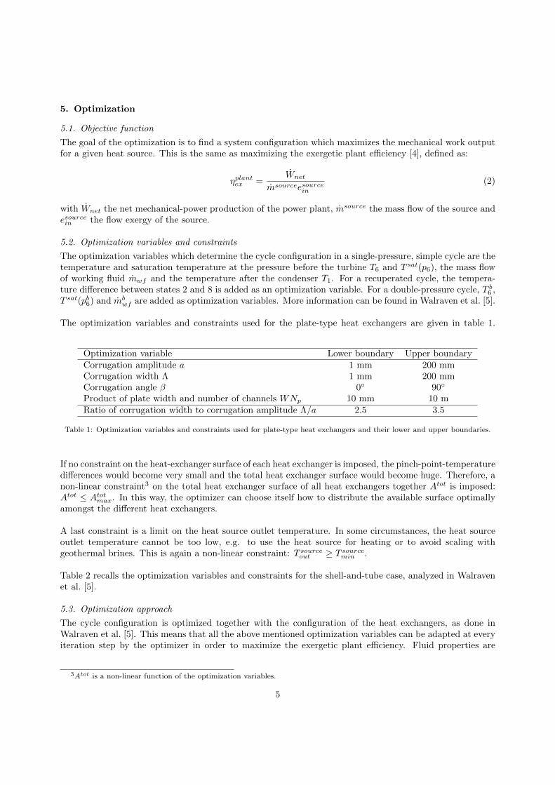
The optimization variables and constraints used for the plate-type heat exchangers are given in table 1.

Optimization variable Lower boundary Upper boundaryCorrugation amplitude a 1 mm 200 mmCorrugation width Λ 1 mm 200 mmCorrugation angle β 0◦ 90◦

Product of plate width and number of channels WNp 10 mm 10 mRatio of corrugation width to corrugation amplitude Λ/a 2.5 3.5

Table 1: Optimization variables and constraints used for plate-type heat exchangers and their lower and upper boundaries.

If no constraint on the heat-exchanger surface of each heat exchanger is imposed, the pinch-point-temperaturedifferences would become very small and the total heat exchanger surface would become huge. Therefore, anon-linear constraint3 on the total heat exchanger surface of all heat exchangers together Atot is imposed:Atot ≤ Atotmax. In this way, the optimizer can choose itself how to distribute the available surface optimallyamongst the different heat exchangers.

A last constraint is a limit on the heat source outlet temperature. In some circumstances, the heat sourceoutlet temperature cannot be too low, e.g. to use the heat source for heating or to avoid scaling withgeothermal brines. This is again a non-linear constraint: T sourceout ≥ T sourcemin .

Table 2 recalls the optimization variables and constraints for the shell-and-tube case, analyzed in Walravenet al. [5].

5.3. Optimization approach

The cycle configuration is optimized together with the configuration of the heat exchangers, as done inWalraven et al. [5]. This means that all the above mentioned optimization variables can be adapted at everyiteration step by the optimizer in order to maximize the exergetic plant efficiency. Fluid properties are

3Atot is a non-linear function of the optimization variables.

5

Optimization variable Lower boundary Upper boundaryShell diameter Ds 0.3 m 2 mTube outside diameter do 5 mm 50 mmRelative tube pitch pt/do 1.15 2.5Relative baffle cut lc/Ds 0.25 0.45Baffle spacing Lb,c 0.3 m 5 mRatio of tube diameter to shell diameter do/Ds / 0.1

Table 2: Optimization variables and constraints used for shell-and-tube heat exchangers and their lower and upper boundaries.

obtained from REFPROP [21] and the complex-step derivative method [22] is used to obtain the derivativeof the fluid properties. These properties are available in Python, in which our model is written, by usingF2PY [23]. The CasADi software [24] calculates the gradient of the objective function and constraintswith automatic differentiation in reverse mode and these gradients are used by the optimizer WORHP [25]together with the value of the objective function to find the optimum.

6. Results

6.1. Reference parameters

100 kg/s of clean water is used as the heat source. The parameters for the reference case are given in table3. The influence of these parameters is investigated in the following sections. The temperature of the heatsource after the ORC is unconstrained and the ORC is of the simple, single-pressure type. In a previouswork [5] it was shown that it is best to use a 30◦- and 60◦-tube configuration in single-phase and two-phaseshell-and-tube heat exchangers, respectively. This combined configuration is used for the comparison in thispaper.

Parameter Symbol ValueHeat source inlet temperature T sourcein 125◦CHeat source mass flow msource 100 kg/sMaximum allowed heat exchanger surface Atotmax 4000 m2

Cooling fluid inlet temperature T coolingin 20◦CCooling fluid mass flow mcooling 800 kg/s

Table 3: Reference parameters.

6.2. Influence maximum allowed heat-exchanger surface

In this section the influence of the maximum allowed heat exchanger surface is investigated. The otherparameters are the ones given in table 3. Figure 4 shows the exergetic plant efficiency for simple ORCswith all plate heat exchangers or all shell-and-tube heat exchangers for different working fluids as a functionof the maximum allowed heat exchanger surface. The efficiency increases with increasing Atotmax, as expected.

This increase of the exergetic plant efficiency with increasing maximum allowed surface is explained bythe increase of the energetic cycle efficiency (figure 5) and the decrease of the heat-source outlet tempera-ture (figure 6). So, more heat is added to the cycle and this heat is converted more efficiently to mechanicalpower when the total heat-exchanger surface increases. This cycle efficiency is defined as:

ηcycleen =Wnet

Q(3)

with Q the heat added to the cycle.

6

2,000 4,000 6,000 8,000 10,000

20

30

40

50

Maximum allowed surface [m2]

plateηplant

ex

[%]

Isobutane Propane

R134a R218

R227ea R245fa

R1234yf RC318

(a) Plate heat exchangers

2,000 4,000 6,000 8,000 10,000

20

30

40

50


shellηplant

ex

[%]

Isobutane Propane

R134a R218

R227ea R245fa

R1234yf RC318

(b) Shell-and-tube heat exchangers

Figure 4: Exergetic plant efficiency for single-pressure, simple ORCs with all plate heat exchangers (a) and all shell-and-tubeheat exchangers (b) for different fluids.

2,000 4,000 6,000 8,000 10,0006

8

10

12


plateηcycle

en

[%]

Isobutane Propane

R134a R218

R227ea R245fa

R1234yf RC318


2,000 4,000 6,000 8,000 10,0006

8

10

12


shellηcycle

en

[%]

Isobutane Propane

R134a R218

R227ea R245fa

R1234yf RC318


Figure 5: Energetic cycle efficiency for single-pressure, simple ORCs with all plate heat exchangers (a) and all shell-and-tubeheat exchangers (b) for different fluids.

For low values of Atotmax ORCs with all plate heat exchangers produce more electrical power than ORCswith all shell-and-tube heat exchangers. It is generally known that plate heat exchangers can achieve higherheat-transfer coefficients and therefore lower pinch-point-temperature differences as seen in figure 7. Forhigh values of Atotmax ORCs with all shell-and-tube heat exchangers perform equally well or even better. Thepinch-point temperature differences in figure 7 become very small and the efficiency of the ORCs almostreaches the upper limit.

7

2,000 4,000 6,000 8,000 10,00040

50

60

70

80

90


plateTout

[◦C

]

Isobutane Propane

R134a R218

R227ea R245fa

R1234yf RC318


2,000 4,000 6,000 8,000 10,00040

50

60

70

80

90


shellTout

[◦C

]

Isobutane Propane

R134a R218

R227ea R245fa

R1234yf RC318


Figure 6: Outlet temperature of the heating fluid for single-pressure, simple ORCs with all plate heat exchangers (a) and allshell-and-tube heat exchangers (b) for different fluids.

For the working fluids R245fa, isobutane and RC318 the exergetic plant efficiency of ORCs with all shell-and-tube heat exchangers is better than the one for ORCs with all plate heat exchangers for Atotmax >2000, 3000 and 6000m2, respectively. Comparison of figures 7a and 7b shows that the pinch-point temper-ature difference between the working fluid and cooling fluid ∆TLowmin decreases much faster in the case ofshell-and-tube heat exchangers with increasing Amax. This is due to fact that the cold and the hot sideof plate heat exchangers with the same number of passes at both sides have exactly the same geometry,which is of course not the case for shell-and-tube heat exchangers. The mass flow of the cooling water ismuch higher than the one of the working fluid, which can result in a large difference between the optimalgeometry of the cold side and the one of the hot side in a plate heat exchanger, leading to relatively highpinch-point-temperature differences.

It can also be noticed from figure 7 that ∆THighmin is lower than ∆TLowmin for subcritical cycles (e.g. Isobutane,R245fa), while they are about equal for transcritical cycles (e.g. R227ea, R1234yf). Because of the highcooling fluid mass flow, ∆TLowmin is relatively close to the average temperature difference, which applies also

to ∆THighmin in transcritical cycles. In subcritical cycles, ∆THighmin is much lower than the average temperaturedifference.

6.3. Influence heat-source inlet temperature

In this section the heat-source inlet temperature is varied between 100 and 150◦C, while keeping the otherparameters constant as given in table 3. It is seen from figure 8 that every fluid performs optimally for acertain heat source-inlet temperature4. ORCs with all shell-and-tube heat exchangers have their maximumplant efficiency at a lower heat-source inlet temperature than plate heat exchangers. A heat source with anhigher inlet temperature contains more energy and more energy will be transfered in the heat exchangers.However, for a fixed maximum allowed heat-exchanger surface, the pinch-point-temperature differences willincrease with increasing heat-source inlet temperature. This increase will in most cases be faster if shell-and-tube heat exchangers are used instead of plate heat exchangers. Higher pinch-point-temperature differences

4For some fluids this optimal temperature is outside the range of the figure

8

2,000 4,000 6,000 8,000 10,0000

5

10

15


plate

∆TLow

min

[◦C

]

Isobutane Propane

R134a R218

R227ea R245fa

R1234yf RC318

(a) Plate heat exchangers, ∆Tmin between working fluidand cooling fluid

2,000 4,000 6,000 8,000 10,0000

5

10

15


shell

∆TLow

min

[◦C

]

Isobutane Propane

R134a R218

R227ea R245fa

R1234yf RC318

(b) Shell-and-tube heat exchangers, ∆Tmin betweenworking fluid and cooling fluid

2,000 4,000 6,000 8,000 10,0000

5

10

15


plate

∆THigh

min

[◦C

]

Isobutane Propane

R134a R218

R227ea R245fa

R1234yf RC318

(c) Plate heat exchangers, ∆Tmin between heating fluidand working fluid

2,000 4,000 6,000 8,000 10,0000

5

10

15


shell

∆THigh

min

[◦C

]

Isobutane Propane

R134a R218

R227ea R245fa

R1234yf RC318

(d) Shell-and-tube heat exchangers, ∆Tmin betweenheating fluid and working fluid

Figure 7: Minimum temperature difference between working fluid & cooling fluid (a,b) and minimum temperature differencebetween heating fluid and working fluid (c,d) for single-pressure, simple ORCs with all plate heat exchangers (a, c) and allshell-and-tube heat exchangers (b, d) for different fluids.

have of course a negative influence on the exergetic plant efficiency and this efficiency will therefore start todecrease earlier when shell-and-tube heat exchangers are used instead of plate heat exchangers.

6.4. Influence heat-source outlet temperature

Often the heat source cannot be cooled down too much; e.g. to avoid scaling in geothermal brines or whenthe heat source after the ORC is used for heating. In this section, the heat-source outlet temperature willbe limited to values between 40 and 90◦C. The other values are the same as in the reference case (table3), but only the results for ORCs with all plate heat exchangers are given. Both simple and recuperated,single-pressure cycles are investigated.

9

100 110 120 130 140 150

30

35

40

45

Heat source inlet temperature [◦C]

plateηplant

ex

[%]

Isobutane Propane R134a

R218 R227ea R245fa

R1234yf RC318


100 110 120 130 140 150

30

35

40

45

Heat source inlet temperature [◦C]

shellηplant

ex

[%]


R218 R227ea R245fa

R1234yf RC318


Figure 8: Exergetic plant efficiency for single-pressure, simple ORCs with all plate heat exchangers (a) and all shell-and-tubeheat exchangers (b) for different fluids. The parameters are those of Table 3.

40 50 60 70 80 90

100

110

120

130

Heat source outlet temperature [◦C]

plate

recupηplant

ex

/plate

standardηplant

ex

[%] Isobutane Propane

R134a R218

R227ea R245fa

R1234yf RC318

(a) Simple cycle

40 50 60 70 80 90

100

110

120

130

Heat source outlet temperature [◦C]

shell

recupηplant

ex

/shell

standardηplant

ex

[%] Isobutane Propane

R134a R218

R227ea R245fa

R1234yf RC318

(b) Recuperated cycle

Figure 9: Exergetic plant efficiency for single-pressure, simple ORCs (a) and recuperated ORCs (b) with all plate heat ex-changers for different fluids. Other parameters are those of Table 3.

Figure 9 shows the comparison between simple and recuperated cycles. When the heat-source outlet tem-perature is limited to a relatively low temperature, both type of cycles perform equally wel as explained inWalraven et al. [4]. When the limit is set at a higher temperature, the recuperated cycles perform betterthan the simple ones. The internal heat recuperation increases the cycle efficiency, which leads to a higherplant efficiency for a fixed heat-source outlet temperature.

10

10 15 20 25 30 35 4020

30

40

50

Cooling fluid inlet temperature [◦C]

plateηplant

ex

[%]

Isobutane Propane

R134a R218

R227ea R245fa

R1234yf RC318

(a) Exergetic plant efficiency

10 15 20 25 30 35 400

2

4

6

8

Cooling fluid inlet temperature [◦C]plate

∆TLow

min

[◦C

]


R218 R227ea R245fa

R1234yf RC318

(b) ∆Tmin between working fluid and cooling fluid

Figure 10: Exergetic plant efficiency (a) and ∆TLowmin (b) for single-pressure, simple ORCs with all plate heat exchangers for

different fluids. Other parameters are those of Table 3.

6.5. Influence cooling-fluid inlet temperature

The cooling-fluid inlet temperature is varied between 10 and 40◦C, while keeping the other parametersconstant (table 3). Only the results for ORCs with all plate heat exchangers are given, because the resultsin the case of all shell-and-tube heat exchangers show the same trend. The exergetic plant efficiency decreaseslinearly as shown in figure 10a, but the decrease is less strong than in the case when ideal components –the results of the ideal case are shown in Walraven et al. [4] – are used. Figure 10b shows the pinch-point-temperature difference between the working fluid and the cooling fluid. This temperature difference decreaseswith increasing cooling-water inlet temperature, so that the condenser temperature remains relatively low.

6.6. Influence cooling-fluid mass flow

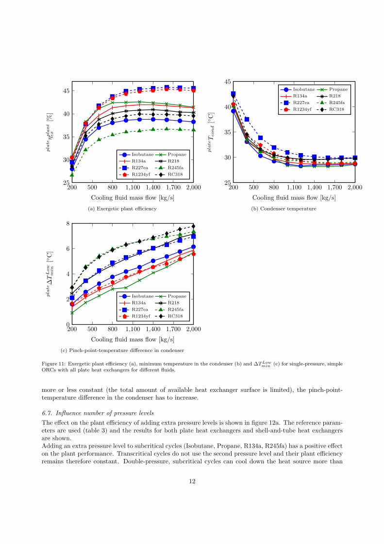
In this section the cooling-water mass flow is varied between 200 and 2000 kg/s. The other parameters aregiven in table 3 and only the results for ORCs with all plate heat exchangers are shown; the results forORCs with all shell-and-tube heat exchangers are analogous. Figure 11a shows the exergetic plant efficiencyas a function of the cooling-water mass flow. At low values of the cooling-water mass flow, an increaseof this mass flow will lead to an increase in the plant efficiency. This efficiency reaches a maximum for amass flow of about 800 kg/s for ORCs with Propane and for a mass flow of about 1100 kg/s for ORCswith Isobutane, R134a, R218 and RC318. For the other investigated fluids the maximum is reached athigher mass flows. The same effect is also seen when shell-and-tube heat exchangers are used, but it isthen less strong. The maximum in the exergetic plant efficiency at a certain mass flow rate is explainedby figure 11b, which shows the minimum temperature in the condenser. This temperature decreases withincreasing cooling water mass flow, which results in a better plant efficiency. The pressure drop in thecooling water increases on the other hand. The combination of the increasing pressure drop and increasingmass flow results in an increasing pumping power. This effect becomes more important than the decreasingcondenser temperature, which results in a maximum plant efficiency for a certain cooling fluid mass flow rate.

Figure 11c shows the pinch-point-temperature difference in the condenser. If the cooling fluid mass flow rateincreases, the cooling-fluid outlet temperature will decrease and the curve of the cooling fluid will becomeflatter in a temperature-heat diagram. In order to keep the average temperature difference in the condenser

11

200 500 800 1,100 1,400 1,700 2,00025

30

35

40

45

Cooling fluid mass flow [kg/s]

plateηplant

ex

[%]

Isobutane Propane

R134a R218

R227ea R245fa

R1234yf RC318


200 500 800 1,100 1,400 1,700 2,00025

30

35

40

45


plateTcond

[◦C

]

Isobutane Propane

R134a R218

R227ea R245fa

R1234yf RC318

(b) Condenser temperature

200 500 800 1,100 1,400 1,700 2,0000

2

4

6

8


plate

∆TLow

min

[◦C

]

Isobutane Propane

R134a R218

R227ea R245fa

R1234yf RC318

(c) Pinch-point-temperature difference in condenser

Figure 11: Exergetic plant efficiency (a), minimum temperature in the condenser (b) and ∆TLowmin (c) for single-pressure, simple

ORCs with all plate heat exchangers for different fluids.

more or less constant (the total amount of available heat exchanger surface is limited), the pinch-point-temperature difference in the condenser has to increase.

6.7. Influence number of pressure levels

The effect on the plant efficiency of adding extra pressure levels is shown in figure 12a. The reference param-eters are used (table 3) and the results for both plate heat exchangers and shell-and-tube heat exchangersare shown.Adding an extra pressure level to subcritical cycles (Isobutane, Propane, R134a, R245fa) has a positive effecton the plant performance. Transcritical cycles do not use the second pressure level and their plant efficiencyremains therefore constant. Double-pressure, subcritical cycles can cool down the heat source more than

12

Isob

uta

ne

Pro

pan

e

R13

4a

R218

R22

7ea

R245f

a

R12

34yf

RC

318

30

35

40

45

ηplant

ex

[%]

1 pressure shell 2 pressures shell

1 pressure plate 2 pressures plate


Isob

uta

ne

Pro

pan

e

R13

4a

R218

R22

7ea

R245f

a

R1234yf

RC

318

40

50

60

70

Tout

[◦C

]

1 pressure shell 2 pressures shell

1 pressure plate 2 pressures plate

(b) Outlet temperature

Figure 12: Exergetic plant efficiency (a) and heat source outlet temperature (b) for simple ORCs with all plate heat exchangersor all shell-and-tube heat exchangers for different fluids.

single-pressure subcritical cycles (figure 12b) and obtain better plant efficiencies, while the energetic cycleefficiency remains about constant when adding a second pressure level.

7. Conclusions

The system optimization of different configurations of ORCs with both plate heat exchangers and shell-and-tube heat exchangers is compared in this paper. Models for heat exchangers used in single-phase flow,evaporation and condensation which are available in the literature are implemented and added to a previousdeveloped ORC-model.

It is shown that ORCs with all plate heat exchangers perform mostly better than ORCs with all shell-and-tube heat exchangers. The disadvantage of plate heat exchangers with an equal number of passes atboth sides of the exchanger is that the geometry of both sides of the heat exchanger are identical, which canlead to an inefficient heat exchanger when the two fluid streams require strongly different channel geometries.

The influence of the maximum allowed heat-exchanger surface, heat-source inlet temperature, constrainton the heat-source outlet temperature, cooling-fluid inlet temperature and mass flow and the number ofpressure levels on the performance of the ORC have been investigated. It is shown that the efficiency of anORC increases with increasing heat-exchanger surface and that every fluid has a heat-source inlet temper-ature for which the plant efficiency is maximal. Recuperated ORCs are only useful when the heat-sourceoutlet temperature is constrained and the best double-pressure subcritical ORCs perform better than thebest single-pressure transcritical cycles.

The cooling-fluid inlet temperature and mass flow have a strong influence on the performance of the ORC.The next step in the system optimization is to model the cooling system and to include it in the optimization.

13

Nomenclature

Greek

β Corrugation angle [◦]∆p Pressure drop [Pa]∆T Temperature difference [◦C]η Efficiency [-]Λ Corrugation width [m]µ Dynamic viscosity [Pa s]Φ Area enlargment factor [-]ρ Density [kg/m3]θ Angle [◦]

14

Roman

a Corrugation amplitude [m]A Area [m2]Bo Boiling number [-]cp Specific eat capacity [J/kgK]do Tube outside diameter [m]D Diameter [m]e Specific exergy [kJ/kg]G Mass velocity [kg/m2s]h Heat transfer coefficient [W/m2K]

Specific enthalpy [J/kg]lc Baffle cut length [m]Lb Distance between baffles [m]Lh Length of a plate [m]Lp Distance between ports [m]m Mass flow [kg/s]Nu Nusselt number [-]p Pressure [bar]Pr Prandtl number [-]pt Tube pitch [m]

Q Heat flow [kW]Re Reynolds number [-]T Temperature [◦C]W Plate width [m]

W Mechanical power [kW]X Corrugation parameter [-]

15

Sub-and superscripts

0 Dead state1− 9 Number of the stateac Accelerationcycle Cycleen Energeticex Exergeticfr Frictionalh Hydraulicid Idealin Inletmax Maximummin Minimumnet Nettl Longitudinalotl Outermost tubesout Outletplant Plants Shellsource Heat sourcet Transversetot Totalwf Working fluid

Acknowledgments

Daniel Walraven is supported by a VITO doctoral grant. The valuable discussions on optimization withJoris Gillis (KU Leuven) are gratefully acknowledged and highly appreciated.

References

[1] J. Tester, B. Anderson, A. Batchelor, D. Blackwell, R. DiPippo, E. Drake, J. Garnish, B. Livesay, M. Moore, K. Nichols,The Future of Geothermal Energy: Impact of Enhanced Geothermal Systems (EGS) on the United States in the 21stCentury, Tech. Rep., Massachusetts Institute of Technology, Massachusetts, USA, 2006.

[2] Y. Dai, J. Wang, L. Gao, Parametric optimization and comparative study of organic Rankine cycle (ORC) for low gradewaste heat recovery, Energy Conversion and Management 50 (3) (2009) 576–582.

[3] B. Saleh, G. Koglbauer, M. Wendland, J. Fischer, Working fluids for low-temperature organic Rankine cycles, Energy32 (7) (2007) 1210–1221.

[4] D. Walraven, B. Laenen, W. Dhaeseleer, Comparison of thermodynamic cycles for power production from low-temperaturegeothermal heat sources, Energy Conversion and Management 66 (2013) 220–233.

[5] D. Walraven, B. Laenen, W. Dhaeseleer, Optimum configuration of shell-and-tube heat exchangers for the use in low-temperature organic Rankine cycles, Energy Conversion and Management 83 (2014) 177–187.

[6] H. Madhawa Hettiarachchi, M. Golubovic, W. M. Worek, Y. Ikegami, Optimum design criteria for an organic Rankinecycle using low-temperature geothermal heat sources, Energy 32 (9) (2007) 1698–1706.

[7] S. Quoilin, V. Lemort, J. Lebrun, Experimental study and modeling of an Organic Rankine Cycle using scroll expander,Applied Energy 87 (4) (2010) 1260–1268.

[8] Z. Shengjun, W. Huaixin, G. Tao, Performance comparison and parametric optimization of subcritical Organic RankineCycle (ORC) and transcritical power cycle system for low-temperature geothermal power generation, Applied Energy88 (8) (2011) 2740–2754.

[9] A. Domingues, H. Santos, M. Costa, Analysis of vehicle exhaust waste heat recovery potential using a Rankine cycle,Energy 49 (2013) 71–85.

[10] A. Franco, M. Villani, Optimal design of binary cycle power plants for water-dominated, medium-temperature geothermalfields, Geothermics 38 (4) (2009) 379–391.

[11] G. F. Hewitt, Hemisphere handbook of heat exchanger design, Hemisphere Publishing Corporation New York, 1990.

16

[12] R. K. Shah, D. P. Sekulic, Fundamentals of heat exchanger design, John Wiley and Sons, Inc., 2003.[13] H. Martin, A theoretical approach to predict the performance of chevron-type plate heat exchangers, Chemical Engineering

and Processing 35 (4) (1996) 301–310.[14] Z. H. Ayub, Plate heat exchanger literature survey and new heat transfer and pressure drop correlations for refrigerant

evaporators, Heat Transfer Engineering 24 (5) (2003) 3–16.[15] E. Djordjevic, S. Kabelac, Flow boiling of R134a and ammonia in a plate heat exchanger, International Journal of Heat

and Mass Transfer 51 (25) (2008) 6235–6242.[16] D.-H. Han, K.-J. Lee, Y.-H. Kim, Experiments on the characteristics of evaporation of R410A in brazed plate heat

exchangers with different geometric configurations, Applied Thermal Engineering 23 (10) (2003) 1209–1225.[17] D.-H. Han, K.-J. Lee, Y.-H. Kim, The characteristics of condensation in brazed plate heat exchangers with different

chevron angles, Journal of the Korean Physical Society 43 (2003) 66–73.[18] A. Jokar, M. H. Hosni, S. J. Eckels, Dimensional analysis on the evaporation and condensation of refrigerant R-134a in

minichannel plate heat exchangers, Applied thermal engineering 26 (17) (2006) 2287–2300.[19] G. A. Longo, R410A condensation inside a commercial brazed plate heat exchanger, Experimental Thermal and Fluid

Science 33 (2) (2009) 284–291.[20] B. Thonon, A. Bontemps, Condensation of pure and mixture of hydrocarbons in a compact heat exchanger: experiments

and modelling, Heat transfer engineering 23 (6) (2002) 3–17.[21] E. Lemmon, M. Huber, M. Mclinden, NIST Reference Fluid Thermodynamic and Transport Properties REFPROP, The

National Institute of Standards and Technology (NIST), version 8.0, 2007.[22] J. R. Martins, P. Sturdza, J. J. Alonso, The complex-step derivative approximation, ACM Transactions on Mathematical

Software (TOMS) 29 (3) (2003) 245–262.[23] P. Peterson, F2PY: a tool for connecting Fortran and Python programs, International Journal of Computational Science

and Engineering 4 (4) (2009) 296–305.[24] J. Andersson, J. Akesson, M. Diehl, CasADi – A symbolic package for automatic differentiation and optimal control, in:

S. Forth, P. Hovland, E. Phipps, J. Utke, A. Walther (Eds.), Recent Advances in Algorithmic Differentiation, vol. 87 ofLecture Notes in Computational Science and Engineering, Springer Berlin Heidelberg, 297–307, 2012.

[25] C. Buskens, D. Wassel, The ESA NLP Solver WORHP, in: Modeling and Optimization in Space Engineering, Springer,85–110, 2013.

Appendix A. Heat transfer and pressure drop correlations

The heat-transfer and pressure-drop correlations used in this paper are given in this appendix.

A.1. Single-phase heat transfer and pressure drop

The model of Martin [13] is used to calculate the pressure drop and heat transfer coefficient in chevron-typeplate heat exchangers for single-phase flows. The frictional-pressure drop for single-phase flow in one plateis given by: [

∆pplatesingle

]fr

= 4fplatesingleLp

Dh

G2

2ρ, (A.1)

with fplatesingle the Fanning friction factor, G = m2aWNp

the mass velocity and Np the number of channels. The

Fanning friction factor is given by:

1√fplatesingle

=cosβ(

0.045 tanβ + 0.09 sinβ + f0cos β

)0.5 +1− cosβ√

3.8f1

, (A.2)

with f0 the Fanning friction coefficient if β = 0◦ and f1 the Fanning friction coefficient if β = 90◦. Thesecoefficients are given by:

f0 =

{16Re for Re < 2000(1.56 lnRe− 3.0)−2 for Re ≥ 2000

, (A.3)

f1 =

149.25Re + 0.9625 for Re < 2000

9.75Re0.289 for Re ≥ 2000

, (A.4)

where Re = GDh

µ is the Reynolds number.

17

The hydrostatic-pressure drop is neglected because the fluids flow alternately up and down and the hydro-static pressure drop is therefore alternately positive and negative. Both are about equal and can thereforebe assumed to neutralize each other.

The heat-transfer coefficient is calculated as:

h =k

Dh0.205Pr1/3

(µmµw

)1/6

(fplatesingleRe2 sin 2β)0.374, (A.5)

with µm the viscosity of the bulk fluid and µw the viscosity of the fluid at the wall. The difference betweenthese viscosities is neglected. Pr is the Prandtl number.

A.2. Heat transfer and pressure drop while evaporating

Han et al. [16] developed correlations for the pressure drop and heat transfer in chevron-type plate heatexchangers during evaporation. The frictional pressure drop in one plate during evaporation is:[

∆pplateevap

]fr

= 4fplateevap Lp

Dh

G2eq

2ρl, (A.6)

with Geq the equivalent mass velocity, defined as:

Geq = G[1− x+ x (ρl/ρv)

1/2], (A.7)

where ρl and ρv are the densities of saturated liquid and saturated vapor, respectively.The correlation for the Fanning friction factor is given by:

fplateevap = c1Rec2eq, (A.8)

with

c1 = 64 710

(Λ

Dh

)−5.27

β−3.03, (A.9)

c2 = −1.314

(Λ

Dh

)−0.62

β−0.47, (A.10)

Reeq =GeqDh

µl. (A.11)

The acceleration pressure drop is given by:

ac∆pplateevap =

(G2eqx

ρl − ρv

)out

−

(G2eqx

ρl − ρv

)in

. (A.12)

The heat transfer coefficient is correlated as:

h =k

Dhc3Re

c4eqBo

0.3eq Pr

0.4l , (A.13)

with:

c3 = 2.81

(Λ

Dh

)−0.041

β−2.83, (A.14)

c4 = 0.746

(Λ

Dh

)−0.082

β0.61, (A.15)

Boeq =q

Geq(hv − hl). (A.16)

18

Boeq is the equivalent boiling number.

The experiments performed by Han et al. [16] were done for β = 45, 55 and 70◦, G = 13 - 34 kg/m2sand a heat flux of 2.5 - 8.5 kW/m2, while using R22 and R410a as working fluids.

A.3. Heat transfer and pressure drop while condensing

The correlations for the pressure drop and the heat transfer coefficient while condensing are given by Hanet al. [17] and are analogous to the ones for the evaporation, albeit with differently defined coefficients ciand h:

[∆pplatecond

]fr

= 4fplatecond LpDh

G2eq

2ρl, (A.17)

fplatecond = c5Rec6eq, (A.18)

c5 = 3521.1

(Λ

Dh

)4.17

β−7.75, (A.19)

c6 = −1.024

(Λ

Dh

)0.0925

β−1.3, (A.20)

h =k

Dhc7Re

c8eqPr

1/3l , (A.21)

c7 = 11.22

(Λ

Dh

)−2.83

β−4.5, (A.22)

c8 = 0.35

(Λ

Dh

)0.23

β1.48. (A.23)

The experiments performed by Han et al. [17] were done for β = 45, 55 and 70◦ and G = 13 - 34 kg/m2s,while using R22 and R410a as working fluids.

19

comparison of shell-and-tube with plate heat exchangers ... · in this paper, the con guration of...

Documents