comparison of software architecture reverse engineering methods
TRANSCRIPT

Comparison of Software Architecture Reverse
Engineering Methods
C. Stringfellow, C. D. Amory, D. Potnuri
Department of Computer Science, Midwestern State University
Wichita Falls, TX 76308, USA
+1 940-397-4578(ph) +1 940-397-4442(fax)
A. Andrews
Electrical Engineering and Computer Science Department, Washington StateUniversity
Pullman, WA 99164, USA
+1 509-335-8656(ph) +1 509-335-3818(fax)
M. Georg
Department of Computer Science and Engineering, Washington University at St.Louis
St. Louis, MO 63130, USA
Abstract
Problems related to interactions between components is a sign of problems withthe software architecture of the system and are often costly to fix. Thus it is verydesirable to identify potential architectural problems and track them across releasesto see whether some relationships between components are repeatedly change-prone.
This paper shows a study of combining two technologies for software architecture:architecture recovery and change dependendcy analysis based on version control in-formation. More specifically, it describes a reverse engineering method to derive achange architecture from Revision Control System (RCS) change history. It com-pares this method to other reverse engineering methods used to derive softwarearchitectures using other types of data. These techniques are illustrated in a casestudy on a large commercial system consisting of over 800 KLOC of C, C++, andmicrocode. The results show identifiable problems with a subset of the componentsand relationships between them, indicating systemic problems with the underlyingarchitecture.
Key words: software architecture, reverse engineering, maintainability
Preprint submitted to Elsevier Science

1 Introduction
As a system evolves and goes through a number of maintenance releases [13],it naturally inherits functionality and characteristics from previous releases[25,26], and becomes a legacy system. As new functionality and features areadded, there is a tendency towards increased complexity. This may impact thesystem’s maintainability. This makes it important to track the evolution of asystem and its components, particularly those components that are becomingincreasingly difficult to maintain as changes are made over time. (Componentsare defined as a collection of files that are logically or physically related.)Increasing difficulty in further evolution and maintenance is a sign of codedecay.
The identification of these components serves two objectives. First, this in-formation can be used to direct efforts when a new system release is beingdeveloped. This could mean applying a more thorough development process,or assigning the most experienced developers to these difficult components.Secondly, the information can be used when determining which componentsneed to be re-engineered at some point in the future. Components that aredifficult to maintain are certainly candidates for re-engineering efforts.
Early decay identification is desirable so that steps can be taken to prevent fur-ther degradation. The question is how to identify this decay and what to do tostop it. Change reports are a major source of commonly available informationthat can be used to identify decay. Change reports are written when develop-ers modify code during system development or maintenance. Change reportsusually contain information about the nature, time and author of the change.A change can modify code in one or more components. If changes are local toa component, that is, only files belonging to the component are changed, thecomponent’s change is said to have cohesion. By contrast, if changes involvemultiple components, the change shows coupling. This concept of looking at achange as either local to a component or as coupling components with regardsto code modification is analogous to describing structure or architecture ofsoftware [1,35]: Software architecture consists of a description of componentsand their relationships and interactions, both statically and behaviorally [35].Problems and possible architectural decay can be spotted via changes related
Email addresses: [email protected], [email protected],
d [email protected] (C. Stringfellow, C. D. Amory, D. Potnuri),[email protected] (A. Andrews), [email protected] (M. Georg).
2

to components and interactions of the components. A software architecturedecay analysis technique must identify and highlight problematic componentsand relationships.
Code decay can be due to the deterioration of a single component. In thiscase it manifests itself in repeated and increasing problems that are local tothe component. A second type of code decay is due to repeated problems thatbecome increasingly difficult to fix and are related to interactions betweencomponents, that is, components are repeatedly fault-prone or change-pronein their relationships with each other. The latter requires changes to code inmultiple components and is a sign of problems with the software architectureof the system. Software architecture problems are by far more costly to fixand thus it is very desirable to identify potential architectural problems earlyand to track them across multiple releases.
High change cohesion and coupling measures indicate problems, although ofa different sort. High change cohesion measures identify components that arebroken in their functionality, while high change coupling measures highlightbroken relationships between components.
There are choices as to which cohesion and coupling measures to use. Ohlssonet al. [32] identify the most problematic components across successive releases,using simple coupling measures based on common code fixes as part of thesame defect report. Von Mayrhauser et al. [39] use a defect coupling measurethat is sensitive to the number of files that had to be fixed in each compo-nent for a particular defect. These defect cohesion and coupling measures canbe computed for all components and components relationships that containfaults. However, usually only the most fault-prone components and compo-nent relationships are of concern, since they represent the worst problems andthe biggest potential for code decay.
Change management data is useful in measuring properties of software changesand such measures can be used in making inferences about cost and changequality in software production. With this in mind, the primary interest is toidentify components and component relationships that exhibit problems mostoften, i.e. with the highest cohesion and coupling measures.
This paper investigates ways to
• identify components and relationships between components that are change-prone or fault-prone either through an existing software architecture docu-ment in conjunction with change history, or, in its absence, through reversearchitecting techniques [4,9,10,14,18,24,40,42]. This paper tries to deal withthe latter situation: an obsolete or missing software architecture documentand the need for some reverse architecture effort. Reverse architecting in thiscontext refers to the identification of a system’s components and component
3

relationships without the aid of an existing architecture document.• measure cohesion and coupling for the components and component relation-
ships identified.• set thresholds for these measures to determine the most problematic com-
ponents and component relationships. The components and component re-lationships that are change-prone form the part of the software architecturethat is problematic. This is called the change architecture.
• verify the change architecture by comparing it to the system architecturederived using reverse architecting techniques that involve #include state-ments similar to the method described in [9,14,18,24], as well as the faultarchitecture [39,36].
Section 2 reports on existing work related to identifying (repeatedly) fault-prone components. It also summarizes existing classes of reverse architectingapproaches. Few researchers have tried to combine the two [11,12]. This paperuses two steps rather than a combination, because the reverse architectingapproach is used to build both a change architecture and a reverse architecture.Section 3 details the approaches used. Section 4 reports on their applicationto a sizable embedded system. The results show identifiable problems with asubset of the components and relationships between them, indicating systemicproblems with the underlying architecture. Section 5 draws conclusions andpoints out further work.
Being able to identify troublesome components is important to determine whatcomponents should be focused on the most in system test or maintenance. Thisstudy uses data extracted from an RCS version control system and its files.This paper ranks components, with the intention of identifying those mostin need of attention. It also identifies which components tend to be changedtogether, whether for fixes or for other reasons. Components that are likelyto change and usually involve changes to a number of other components needspecial attention to ensure that the job is done right. The methods describedin this paper will identify components that have many relationships betweenfiles within their own component and with other components. The architecturediagrams created will visually display those problematic components.
2 Background
2.1 Tracking and Predicting Fault-prone Components
It is important to know which software components are stable versus thosewhich repeatedly need corrective maintenance, because of decay. Decayingcomponents become worse as they evolve over releases. Software may decay
4

due to adding new functionality with increasing complexity as a result ofpoor documentation of the system. Over time decay can become very costly.Therefore it is necessary to track the evolution of systems and to analyzecauses for decay.
Ash et al. [2] provide mechanisms to track fault-prone components across re-leases. Schneidewind [34], Khoshgoftaar et al. [21] provide methods to predictwhether a component will be fault-prone. Khoshgoftaar et al. [22] present analgorithm using a classification tree, which represents an abstract tree of deci-sion rules to aid in classifying fault-prone models. Their results show that theclassification-tree modeling technique is robust for building software qualitymodels. They also show that principal component analysis can improve theclassification-tree model to classify fault-prone modules.
Ohlsson et al. [32,31] combine prediction of fault-prone components with anal-ysis of decay indicators. It ranks components based on the number of defectsin which a component plays a role. The ranks and changes in ranks are usedto classify components as green, yellow and red (GYR) over a series of re-leases. Corrective maintenance measures are analysed via Principal Compo-nents Analysis (PCA) [15]. This helps to track changes in the componentsover successive releases.
According to Graves et al.[16], software change history is more useful in pre-dicting number of future faults than product measurements of the code, suchas number of lines of code and number of developers. They focus on identi-fying those aspects of the code and its change history that are most closelyrelated to the number of faults that appear in modules of the code. Theirmost successful model measures the fault incidence of a module based on thesum of contributions from all forms of changes, with large and recent changesreceiving most weight.
Graves and Mockus [17] describe a methodology for historical analysis of theeffort necessary for developers to make changes to software. The results of thestudy show that four types of variables are critical contributors to estimatedchange effort: the size of the change, the developer making the change, thepurpose of the change, and the date the change was opened. The conclusionsdrawn from this study are important as they can be used in project manage-ment tools to (1) identify modules of code which are too costly to change, or(2) assess developers’ expertise with different modules.
Ostrand and Weyuker [33] examine the relationship between fault-pronenessand the age of the file, the relationship between a file’s change status and itsfault-proneness, and to what extent the system’s maturity affects the faultdensity. They observe that the age of a file is not a good predictor of fault-proneness: as the product matured the overall system fault density decreased.
5

Their results show that testers need to put more effort on new files, ratherthan on files that already exist.
Tools and a sequence of visualizations and visual metaphors can help engineersunderstand and manage the software change process. In [29], Mockus et al.describe a web-based tool, which is used to automate the change measurementand analysis process. The change measures include change size, complexity,purpose and developer expertise. Version control and configuration manage-ment databases provide the main sources of information. Eick et al. [6] presentsseveral useful metaphors: matrix views, cityscapes, charts, data sheets, andnetworks, which are then combined to form ”perspectives”. Different waysto visualize the changes and the components changed are also categorized.Changes are classified as adaptive, corrective, and perfective maintenance.The goal is to understand the relationship between dimensions (attributesassociated with the software development process that cannot be controlled)and measures (the responses that the development organization wishes to un-derstand and control). The authors conclude there are significant payoffs -both intellectual and economic - in understanding change well and managingit effectively.
2.2 Reverse architecture
Reverse architecting is a specific type of reverse engineering. According to [19],a reverse engineering approach should consist of the following:
(1) Extraction: This phase extracts information from source code, documen-tation, and documented system history (e. g. defect reports, change man-agement data).
(2) Abstraction: This phase abstracts the extracted information based on theobjectives of the reverse engineering activity. Abstraction should distillthe possibly very large amount of extracted information into a manage-able amount.
(3) Presentation: This phase transforms abstracted data into a representationthat is conducive to the user.
Objectives for reverse architecting code drives what is extracted, how it isabstracted, and how it is presented. For example, if the objective is to re-verse architect with the associated goal to re-engineer (let’s say into an objectoriented product), architecture extraction is likely based on identifying and ab-stracting implicit objects, abstract data types, and their instances [4,14,18,40].Alternatively, if it can be assumed that the code embodies certain architec-tural cliches, an associated reverse architecting approach would include theirrecognition [10].
6

Other ways to look at reverse architecting a system include using state ma-chine information [12], or release history [11]. CAESAR [11] uses the releasehistory for a system. It tries to capture logical dependencies instead of syn-tactic dependencies by analyzing common change patterns for components.This allows identification of dependencies that would not have been discov-ered through source code analysis. It requires data from many releases. Thismethod could be seen as a combination of identification of problematic com-ponents and architectural recovery to identify architectural problems.
If one is interested in a high level fault architecture of the system, it is desirablenot to extract too much information during phase 1, otherwise there is eithertoo much information to abstract, or the information becomes overwhelm-ing for large systems. This makes the simpler approaches more appealing. Inthis regard, Krikhaar’s approach is particularly attractive [24]. The approachconsists of three steps:
(1) Define and analyze the import relation (via #include statements) betweenfiles[24]. Each file is assigned to a subsystem (in effect creating a part-ofrelation). If two files in different subsystems have an import relationship,the two subsystems to which the files belong have one as well.
(2) Analyze the part-of hierarchy in more general terms (such as clusteringlevels of subsystems). This includes defining the part-of relations at eachlevel.
(3) Analyze use relations at the code level. Examples include call-called byrelationships, definition versus use of global or shared variables, constantsand structures. Analogous to the other steps, Krikhaar [24] abstracts userelations to higher levels of abstraction.
Within this general framework, there are many options to adapt it to a specificreverse architecting objective [9]. For example, the method proposed by Bow-man et al. [3] fits into this framework: the reverse architecting starts with iden-tifying components as clusters of files. Import relations between componentsare defined through common authorship of files in the components (ownershiprelation). Bowman et al. [3] also includes an evaluation of how well ownershipand dependency relationships model the conceptual relationship.
2.3 Version history analysis
Several recent studies [3,5,7,8,27,30,37,41,44] have focused on version historyanalysis to identify components that may need special attention in some main-tenance task. Fischer et al. [7,8] describe an approach for populating a releasehistory database with data from bug tracking and version control systems tounderstand the evolution of a software system. They look at problem reports
7

and modification reports for software features to uncover hidden relationshipsbetween the features. Visualization of these relationships can aid in identifyingareas of design erosion (or code decay). Ying et al. [41] and Zimmerman etal. [44] develop approaches that use association rule mining on a software con-figuration management system (CVS) to observe change patterns that involvemultiple files. These patterns can guide software developers to other poten-tial modifications that need to be made to other files. Mockus and Weiss [27]introduce methods that uses modification requests to identify tightly coupledwork items as candidates for independent development, especially useful whendevelopers are at different sites. Stringfellow et al. [37] use change history datato determine the level of coupling between components to identify potentialcode decay.
Most of these approaches require grouping changes that are made to code insome way. Changes may be grouped according to a common author and a smalltime interval for checking in the changed files [5,27,37]. Ying et al. [41] alsorequire the same check-in comment. Changes may also be grouped accordingto check in times for files changed to fix the same defect or respond to the sameproblem report [8]. The time intervals used to group changes vary. Curbranicand Murphy [5] group check ins that occur within six hours, but indicateconfidence in the grouping decreases after five minutes. Zimmerman et al. [44]propose using a time interval of 3 1/3 minutes. Most of these approaches areat the file level [5,7,8,37,41], while some are finer-grained [27,44].
This paper uses an adaption of the reverse architecture technique proposedin [9] using version control history to build a change architecture. A changegroup consists of file changes that are checked in by the same author withina certain time interval. Different time intervals are considered. This analysisis lifted to the component level to derive a change architecture. In addition,a ”fault architecture” is derived taking into consideration changes made tofiles for purposes of fixing a common defect, the author of the change, and thecheck-in time of files changed. These architectures are analyzed and comparedto a reverse architecture based on #include statements similar to [9].
3 Approach
A software developer needs to focus on the most problematic parts of the ar-chitecture in testing or maintenance, those that are most fault-prone and/orchange-prone. This study derives a software architecture using three differentreverse engineering techniques for comparison purposes. The first technique isbased on static relationships - the #include relationships, as described in [9].Other measures of function calls and global variables may also be used, how-ever, this study chose #includes, because the other two techniques work on a
8

file level. The second technique is based on grouping changes to files withinand between components [37]. The third technique groups changes based ona common defect they are meant to fix. The following sections describe thesetechniques in more detail.
3.1 LOC change architecture
Stringfellow et al. [37] describe an approach to derive change architecturesfrom RCS history data. RCS files [38] include the date and time of each check-in, the name of the person who made the change and the number of lines addedand deleted from the file. As source files are checked in and out of RCS, a log isautomatically inserted into the file. Each log in a file has a unique number andincludes the date, time, and author of the change. A perl program traversesthe application system’s directory to search for the source files, open them,and extract information from the logs.
In order to perform any meaningful analysis on that data, all related changesmust be put into the same group. Two assumptions are made to determinewhich changes are related. The first assumption is that all related changes aremade by the same programmer. Secondly, it is assumed that related changesare checked in within a certain time interval.
It is also assumed that components with the highest number of lines of code(LOC) changed in their files are the most likely to require changes, and arehence change-prone. RCS logs contain data on the number of LOCs addedand deleted in each change. Stringfellow et al. [37] use this data in two ways:
• Change Cohesion MeasureTo rank the change-prone components, in terms of local changes. The
change cohesion metric, for a component C, is defined as follows:
Coh(C) = Σni=1 FLOCi (1)
wheren refers to the number of files in a componentFLOCi refers to the number of lines of code changed for each of the n
individual files in component, C.• Change Coupling Measure:
To rank the change-prone relationship of components. The change cou-pling metric is defined, for a pair of components Cj and Ck, as:
Coupling(Cj, Ck) = Σmi=1 GLOCi (2)
where
9

m refers to the number of groups of related changes, where a group is aset of changes checked in to RCS by the same author within a time interval,and
GLOCi refers to the number of lines of code changed in each group ofrelated changes that changed code in both components, Cj and Ck, j 6= k.
Once the measures are collected, change architecture diagrams are created,showing the components and relationships with the highest values, which areconsidered most change-prone. As in [36], the thresholds are set at 10% of thehighest measures.
3.2 Fault architecture
Von Mayrhauser et al. [39] combine the concepts of fault-prone analysis andreverse architecting to determine and analyze the fault-architecture of softwareacross releases. The basic strategy to derive the fault architecture uses defectcohesion measures for components and defect coupling measures between com-ponents to assess how fault-prone components and component relationshipsare. If the objective is to concentrate on the most problematic parts of thesoftware architecture, these measures are used with thresholds to identify
• The most fault-prone components only (setting a threshold based on thedefect cohesion measure);
• The most fault-prone components relationships (setting a threshold basedon two defect coupling measures).
The defect cohesion and coupling measures are defined in [36] as follows:
• Multi-file Defect Cohesion Measure:Multi-file defect cohesion counts the pairwise defect relationships between
files within the same component where those files were changed as part ofa defect repair:
Co<C> =n
∑
i=1
Ci<C>(3)
where
Ci<C>=
1, fdi= 1 and only 1 component is involved in fixing di
fdi(fdi
−1)
2, fdi
≥ 2
andfdi
is the number of files in component C that had to be changed to fixdefect di.
10

n is the number of defects that necessitated changes in component C.
This provides an indication of local fault-proneness. Unless only one file ischanged, this measure will be much larger than the basic cohesion measure.It penalizes components that are only involved in a few defects, but whereeach defect repair involved multiple files.
The defect coupling measures are defined as follows:
• Multi-file Defect Coupling Measure: Two or more components are fault re-lated, if their files had to be changed in the same defect repair (i.e. in orderto correct a defect, files in all these components needed to be changed).
For any two components C1 and C2, the defect coupling measure Re<C1,C2>
is defined as:
Re<C1,C2> =n
∑
i=1
C1di× C2di
, C1 6= C2 (4)
whereC1di
and C2diare the number of files in component C1 and C2 that were
fixed in defect di
n is the number of defects whose fixes necessitated changes in compo-nents C1 and C2.
• Cumulative Defect Coupling Measure: A component C can be fault-pronewith respect to relationships if none of the individual defect coupling mea-sures are high, but there are a large number of them (the sum of the defectcoupling measure is large). In this case the defect coupling measure for acomponent C is defined as:
TRC =m
∑
i=1
Re<C,Ci> C 6= Ci (5)
wherem is the number of components other than CRe<C,Ci
> is the defect coupling measure between C and Ci.
The multi-file defect coupling measure emphasizes pairwise coupling related tocode changes for defects involving a pair of components. The cumulative defectcoupling measure is concerned with components in many fault relationshipswith two or more components.
Stringfellow et al. [36] determine defect cohesion and defect coupling measuresfor all components. Then they filter based on the defect coupling measure tofocus on the most problematic relationships. A component is considered fault-prone in a release, if it is among the top 25% in terms of defect reports writtenagainst the component. The 25% threshold provides a manageable number of
11

problematic components for further analysis. Similarly, a threshold may dis-tinguish between component relationships that are fault-prone and those thatare not. The threshold is set to an order of magnitude less than (or 10% of) themaximum value of the defect coupling measure. Component relationships werefault-prone depending on how often a defect repair involved changes in filesbelonging to multiple components. When identifying fault-prone componentrelationships, the method only identifies components as having fault-prone re-lationships, if these relationships rank in the top 25%. This omits componentsin the fault architecture with fault relationships that rank lower, but whichmay still have a large number of them.
Stringfellow et al. [36] adapted the technique to highlight both the nature andmagnitude of the architectural problem. They include components in the faultarchitecture if the number of fault relationships is within an order of magnitudeof the number of fault relationships of the highest ranked component. Thedefect cohesion measure by Von Mayrhauser et al. [39] does not differentiatebetween defects that require modifying one file in a component, or dozens. Theapproach in Stringfellow et al. [36] distinguishes between single and multiplefile changes related to a defect repair. This provides a ranking of componentswith respect to how locally fault-prone they are and this simplifies issuesrelated to validation of the measures [20].
The fault relationship can be abstracted to the subsystem level: Two subsys-tems are related, if they contain components that are related. This representsKrikhaars lift operation [24]. Von Mayrhauser et al. [39] and Stringfellow etal. [36] apply this lifting method when going from the subsystem to the systemlevel. Changes in patterns, or persistent fault relationships between compo-nents, across releases, are indicators of systemic problems between componentsand thus architecture.
Von Mayrhauser et al. [39] and Stringfellow et al. [36] also produce a seriesof fault architecture diagrams, one for each release. The fault architecturediagrams are aggregated into a Cumulative Release Diagram and show thecomponents that occur in at least one fault architecture diagram [36].
This study works with data from RCS change history and does not includedata from a defect tracking system. Therefore, to derive a ”fault architecture”,changes by the same author and for a time interval are grouped togetherand the changes are assumed to fix a common defect. This allows the faultarchitecture technique described in Stringfellow et al. [36] to be applied.
12

3.3 Comparing architectures
The approach to compare the architectures from process data consists of thefollowing steps:
• Extract desired data from logs in RCS source files.• Group all related changes and create an aggregate change architecture di-
agram for the different time intervals. Change-prone components and re-lationships are identfied by analyzing the number of lines of code (LOCs)changed, as in [37].
• Create a fault architecture diagram by analyzing files changed to fix defects,as in [36].
• Create a reverse architecture diagram by analyzing #include statements infiles, as in [24].
• Compare the architecture diagrams.
Relationships, either change-prone or fault-prone, that appear in change orfault architecture diagrams identify components that are becoming increas-ing difficult to maintain over time. Change-prone or fault-prone ralationshipsbetween components that do not have #incude relationships, especially indi-cate an increased complexity in the system’s architecture that affect futureevolution and maintenance. This is a sign of decay.
The architecture techniques are applied in this study to a large commercialflight simulation system consisting of over 800 KLOC of C, C++, and mi-crocode. The system has 58 components, each of which consists of one to 108files that are logically related. Over half of the components contain 3 files orless. For the purposes of this paper, a component is defined as a set of fileslocated in the same directory. The component files are organized into sev-eral directories with several subdirectories in these directories, every directoryexcept the home directory contains files. Files in the subdirectories of a com-ponent directory are not considered part of the component. Figure 1 shows thedirectory structure of the system. Numbers in the nodes represent the numberof header and source code files in the component.
4 Analysis of architectures
4.1 Reverse architecture
Figure 2 shows the reverse architecture diagram for the flight simulation sys-tem based on #include relationships. This figure focuses on subsystem S3 (a
13

subsystem with many .c and .cpp files). The nodes in the diagram representthe components. Edges represent a relationship between two components. Thestrength of the relationships between components in this diagram are indicatedby the number of #includes. For example, file(s) in component s3/N includefiles from S1 - it might be that one file in S3/N includes 14 different files inS1, or 14 files in S3/N include one file in S1, or several files in S3/N includeseveral files in S1. The layout for this figure also serves as a master for theother architecture diagrams for comparison purposes.
Most of the architectural dependencies are related to header files and corre-sponding source files. Many of the components in S3 include files in compo-nents S1 and S2/I. As it happens, S1 and S2/I contain many of the header files.Few components in Subsystem S3 include files from other components in S3,due to the fact that components in this subsystems tend to implement differ-ent features of the system, so little coupling is expected. Component S3/c doesinclude a file from component S3/w. These components implement features forweapons and countermeasures, and one might expect that a countermeasurecould involve a weapon. Component S2/S/s concerns scenarios, and containsboth the defintion and implementation of scenarios within the same compo-nent. Similarly, components S3/N/d, S3/w, S3/c, and S2/S/l contain headerand corresponding source files.
Figure 3 focuses on the relationships between components in subsystems S2and S3. For example, file(s) in S3/s includes file(s) from S2/p.
Figure 4 shows the #include architecture of the S2 subsystem locally. Theshaded components in the diagram are also in Figure 2. This diagram showsthe internal relationships between components of subsystem S2 and the S2components that include files in the S1 subsystem.
The #include architecture diagrams in this study reveal a great many re-lationships in the system, too many to be understandable. The benefit ofthe #include architecture is mainly to help validate relationships found usingother reverse architecture methods and to aid in the understanding of thoserelationships.
4.2 LOC change architecture
Each RCS file includes data regarding the number, date, time, author, andnature of each change. In addition, the number of lines of code deleted andadded for each change is available. Files that were checked into RCS withina given time interval are considered part of the same group, and are assumedto be related to fixing a particular problem or implementing an additionalfeature.
14

Figure 5 shows the aggregate change architecture diagram using time intervalsof 2 minutes, 7 minutes, 10 minutes and 30 minutes for purposes of groupingcheck-ins. It probably does not make sense to group files checked-in too farapart, as they are most likely not related to fixing one particular problem.The 5 minute interval resulted in the same change-prone relationships as the2 minute interval, so that data is not presented.
A shaded node indicates a component is locally change-prone, that is, itsgrouped changes result in many lines of code changed in files within that com-ponent only. The numbers in brackets in these nodes are the change cohesionmeasures and indicate the number of lines of code changed in files withinthat component, hence they are a local change measure. Locally change-pronecomponents are those whose change cohesion measures are in the top 10%. Fo-cusing attention on these components in testing or maintenance should yieldthe most benefits. Available time and effort may dictate a different threshhold,but this study follows the recommendation in [36] in setting the threshhold.
Regardless of which time interval is used for grouping changes (2 or 30 min-utes), components S2/p, S3/s, S3/N/d, S3/w and S3/a are considered locallychange-prone. Component S3/N/r locally change-prone only in the 2 minuteinterval – it has very close check-in times for files with a large number of LOCchanged. If changes are related by check-in times of more than 5 minutes apart,then S3/N/r is not one of the highest ranking change-prone components. Theassumption, however, is that very close check-in times for files indicates thatthe changes are related.
Components with a high change coupling measure indicate a change-prone re-lationship with another component. The numbers labeling the edges indicatethe number of lines of code changed in files in the components with the changerelationship for 2, 7, 10, and 30 minute intervals. There were over 60 changerelationships between components identified, but the change architecture di-agram focuses on those that have the highest measures. It shows componentswhose change coupling measures are in approximately the top 10% of the rela-tionships in terms of number of lines of code changed. If the change couplingmeasure was not in the top 10a time interval, it is indicated by a ’-’. Thisindicates that for this time interval grouping that the relationship would notbe considered one of the most change-prone.
The change-prone relationships between components S2/p and S2/s, S2/p andS2/I, and S2/s and S2/I occur for all time intervals. Note that S1 does notappear to be in a change-prone relationship for the two minute grouping,but there is a big difference in the number of lines of code changed in thecomponents’ file in the 7 minute group, and then not much more within 10minutes and 30 minutes groups. In the change architecture diagrams thatgroup changes that occurred within 30 minutes, the number of relationships
15
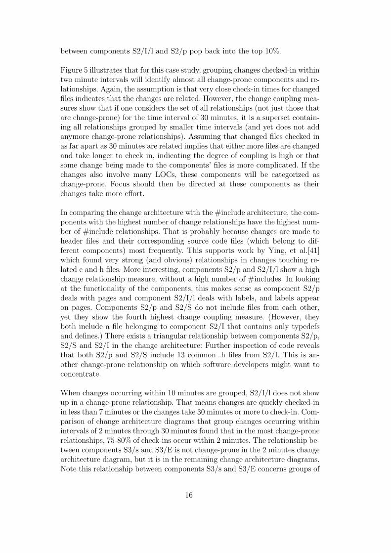
between components S2/I/l and S2/p pop back into the top 10%.
Figure 5 illustrates that for this case study, grouping changes checked-in withintwo minute intervals will identify almost all change-prone components and re-lationships. Again, the assumption is that very close check-in times for changedfiles indicates that the changes are related. However, the change coupling mea-sures show that if one considers the set of all relationships (not just those thatare change-prone) for the time interval of 30 minutes, it is a superset contain-ing all relationships grouped by smaller time intervals (and yet does not addanymore change-prone relationships). Assuming that changed files checked inas far apart as 30 minutes are related implies that either more files are changedand take longer to check in, indicating the degree of coupling is high or thatsome change being made to the components’ files is more complicated. If thechanges also involve many LOCs, these components will be categorized aschange-prone. Focus should then be directed at these components as theirchanges take more effort.
In comparing the change architecture with the #include architecture, the com-ponents with the highest number of change relationships have the highest num-ber of #include relationships. That is probably because changes are made toheader files and their corresponding source code files (which belong to dif-ferent components) most frequently. This supports work by Ying, et al.[41]which found very strong (and obvious) relationships in changes touching re-lated c and h files. More interesting, components S2/p and S2/I/l show a highchange relationship measure, without a high number of #includes. In lookingat the functionality of the components, this makes sense as component S2/pdeals with pages and component S2/I/l deals with labels, and labels appearon pages. Components S2/p and S2/S do not include files from each other,yet they show the fourth highest change coupling measure. (However, theyboth include a file belonging to component S2/I that contains only typedefsand defines.) There exists a triangular relationship between components S2/p,S2/S and S2/I in the change architecture: Further inspection of code revealsthat both S2/p and S2/S include 13 common .h files from S2/I. This is an-other change-prone relationship on which software developers might want toconcentrate.
When changes occurring within 10 minutes are grouped, S2/I/l does not showup in a change-prone relationship. That means changes are quickly checked-inin less than 7 minutes or the changes take 30 minutes or more to check-in. Com-parison of change architecture diagrams that group changes occurring withinintervals of 2 minutes through 30 minutes found that in the most change-pronerelationships, 75-80% of check-ins occur within 2 minutes. The relationship be-tween components S3/s and S3/E is not change-prone in the 2 minutes changearchitecture diagram, but it is in the remaining change architecture diagrams.Note this relationship between components S3/s and S3/E concerns groups of
16

check-ins that are performed by the same programmer within 7 minutes. Ofmost interest, is the change-prone relationship between the components S3/sand S3/E, which do not include any files from each other. In addition, thesetwo components seem to involve very different functionality (one relates tosurfaces and the other to aircraft engine function). Why would a programmerwork on two components that do not include files from one another? Inspec-tion of the relationship between components S3/s and S3/E reveals that bothinclude the same two files from S2/I. This triangular relationship is not visiblein the change architecture diagram.
4.3 Fault architecture
The fault architecture methods employed by Stringfellow et al. [36] are ap-plied to reverse engineer the software architecture for the same flight similatorsystem. Strictly speaking these are not fault architectures, since the data usedis RCS change data, and not defect data. The techniques discussed in [36]assume that data relating to fault architecture are available.
Figure 6 shows components considered to be fault-prone and components infault-prone relationships. Components’ total relationship coupling measures(TRc) and their defect coupling relationship measures (Re) are indicated be-side nodes and on edges. The inset in the figure lists the fault-prone com-ponents that are locally fault-prone, that is in fixing each fault multiple fileswithin the component had to be changed. This figure is derived by groupingfile check-ins in which changes fix a defect using a 15 minute time interval. Inshorter time intervals, the fault-prone relationship between S2/I/s and S2/pdid not exist. A time interval of 20 minutes up to 59 minutes shows one addi-tional fault-prone relationship between components S2/S/s and S2/p. Other-wise, the only differences in the fault-architectures for different time intervalsis an increase in the measures (and not the components).
The fault architecture diagram for this system is very similar to the changearchitecture diagram. This diagram is compared to the diagram in Figure 5.Components S1, S2/p, S3/s, S3/N/d, S3/w, S3/a, S2/I, and S2/S are notonly change-prone; they are also fault-prone. Components S3/E and S2/I/sare considered change-prone, but not fault-prone. Components S3/h, S3/c,S2/S/s, and S3/N/c are fault-prone, but not change-prone.
Relationships that are both fault-prone and change-prone include those be-tween components S1 and S3/s and S2/p and S2/I/s, as well as the triangularrelationship between components S2/p, S2/I, and S2/S. Only one more re-lationship appears to be change-prone and that appears between S3/s andS3/E. The relationships between components S2/p and S2/S/s and S3/N/d
17

and S3/N/r are fault-prone, but not change-prone.
The change architecture diagram indicates the same problematic componentsand component relationships that fault-architecture diagram does. A few prob-lematic components are identified by one method only. This shows that usingeither fault data or change data, one may reverse architect a system andproduce similar architectures identifing the same problematic components. If,however, both fault and change data are available, thorough software devel-opers may want to use both methods to pick up a few more problematiccomponents.
5 Future work
Mockus and Votta[28] hypothesize that one can use the textual descriptionof a software change to derive the reason for that change. Additional futurework with change architecture will involve determining the change architec-ture based on the type of change. Their study also found strong relationshipsbetween the type and size of a change and the time required to carry it out.Future work may focus on changes that take more effort. The change architec-ture diagram shows us that most check-ins for code changes, when grouped byprogrammer and time, are quickly accomplished within two (to five) minutes.The number of lines of code changed does not increase dramatically when look-ing at changes grouped within 30 minutes. More interesting, perhaps, wouldbe to focus on changes that occur within 30 minutes, but exclude all thosethat occur within 2 minutes. These components may be more highly coupled(involving many files) or the changes made to the components’ files are morecomplicated causing some files to be checked in further apart in time.
6 Conclusions
The data used in this study are derived from RCS change history which, by itsvery nature, deals with changes at the file level. This means that any researcherseeking to find component-based changes or change relationships using RCShas to find some means of first determining the files in each component, thenthe various relationships between components. The RCS change history infor-mation for files must be lifted to components: This is not difficult to do witha few scripts, but a configuration management system that stores the historyof components in addition to the files would be helpful.
The #include architecture diagrams in this study reveal a great many re-lationships in the system, too many to be understandable. The benefit of
18

the #include architecture is mainly to help validate relationships found usingother reverse architecture methods and to aid in the understanding of thoserelationships. In this study, most of the change-prone relationships involvecomponents in which one has a .cpp file and the other has the corresponding.h file. These are obvious strong relationships. The change architecture dia-gram and the fault architecture diagram also effectively reveal relationshipsbetween components that are not obvious by looking at the #include archi-tecture diagrams. Both the change and fault architecture methods found thesame triangular relationship, that is not so obvious. Code inspection revealedthat in these relationships, the components have files that include one or two.h files from a third component. The change architecture method also founda relationship between two components implementing very different features.The software developers might want to investigate this unusual coupling.
The results show identifiable problems with a subset of the components andrelationships between them, indicating systemic problems with the underly-ing architecture. By comparing the different software architectures reverseengineered using change or fault data, problematic components and the prob-lematic relationships between them are validated. The change architectureand fault architecture, which focus on a certain percentage of change-prone orfault-prone components and their relationships will allow a software developerto focus attention on these components in testing and maintenance tasks.
References
[1] R. Allen, D. Garlan, Formalizing Architectural Connection, ProceedingsInternational Conference on Software Engineering, IEEE Computer SocietyPress, Los Alamitos CA, 1994, pp. 71-80.
[2] D. Ash, J. Alderete, P. Oman, B. Lowther, Using Software Models to TrackCode Health, Proceedings International Conference on Software Maintenance,IEEE Computer Society Press, Los Alamitos CA, 1994, pp. 154–160.
[3] I. Bowman, R.C. Holt, Software Architecture Recovery Using Conway’s Law,Proceedings CASCON’98, 1998, Mississauga, Ontario, Canada, pp. 123–133.
[4] G. Canfora, A. Cimitile, M. Munro, C. Taylor, Extracting abstract datatypes from C programs: a case study, Proceedings International Conferenceon Software Maintenance, IEEE Computer Society Press, Los Alamitos CA,1993, pp. 200–209.
[5] D. Cubranic, G. Murphy, Hipikat: Recommending pertinent softwaredevelopment artifacts, Proceedings Internations Conference on SoftwareEngineering, IEEE Computer Society Press, Los Alamitos CA, 2003, pp. 408–418.
19

[6] S. Eick, T. Graves, A. Karr, A. Mockus, P. Schuster, Visualizing SoftwareChanges, IEEE Transactions on Software Engineering, 28 4, 2002, pp. 396–412.
[7] M. Fischer, M. Pinzger, H. Gall, Analyzing and relating bug report data forfeature tracking, Proceedings 10th Working Conference on Reverse Engineering,IEEE Computer Society Press, Los Alamitos CA, 2003, pp. 90–101.
[8] M. Fischer, M. Pinzger, H. Gall, Populating a release history database fromversion control and bug tracking systems, Proceedings International Conferenceon Software Maintenance, IEEE Computer Society Press, Los Alamitos CA,2003, pp. 23-33.
[9] L. Feijs, R. Krikhaar, R. van Ommering, A relational approach to softwarearchitecture analysis, Software Practice and Experience, 1998 28(4), pp. 371–400.
[10] R. Fiutem, P. Tonella, G. Antoniol, E. Merlo, A cliche-based environment tosupport architectural reverse engineering, Proceedings International Conferenceon Software Maintenance, IEEE Computer Society Press, Los Alamitos CA,1996, pp. 319–328.
[11] H. Gall, K. Hajek, M. Jazayeri, Detection of logical coupling based on productrelease history, Proceedings International Conference on Software Maintenance,IEEE Computer Society Press, Los Alamitos CA, 1998. pp. 190–198.
[12] H. Gall, M. Jazayeri, R. Kloesch, W. Lugmayr G. Trausmuth, Architecturerecovery in ARES, Proceedings Second International Software ArchitectureWorkshop, ACM Press, New York NY, 1996, pp. 111–115.
[13] D. Gefen, S. Schneberger, The non-homogeneous maintenance periods: acase study of software modifications, Proceedings International Conference onSoftware Maintenance, IEEE Computer Society Press, Los Alamitos CA, 1996,pp. 134–141.
[14] J. Girard, R. Koschke, Finding components in a hierarchy of modules: a steptowards architectural understanding, Proceedings International Conference onSoftware Maintenance, IEEE Computer Society Press, Los Alamitos CA, 1997,pp. 58–65.
[15] R. Gorsuch, Factor Analysis, Second Edition, Laurence Erlbaum Associates,Hillsdale NJ, 1983.
[16] T. Graves, A. Karr, J. Marron, H. Siy, Predicting fault incidence usingsoftware change history, IEEE Transactions on Software Engineering, 26 7,2000, pp. 653–661.
[17] T. Graves, A. Mockus, Inferring Change Effort from Configuration ManagementDatabases, Proceedings of the 5th International Symposium on SoftwareMetrics, Bethesda, MD, 1998, pp. 267–273.
20

[18] D. Harris, A. Yeh, H. Reubenstein, Recognizers for extracting architecturalfeatures from source code, Proceedings Second Working Conference on ReverseEngineering, IEEE Computer Society Press, Los Alamitos CA, 1995, pp. 252–261.
[19] S. Tilley, K. Wong, M. Storey, H. Muller, Programmable reverse engineering,International Journal of Software Engineering and Knowledge Engineering,4(4), 1994, pp. 501–520.
[20] B. Kitchenham, S. Pfleeger, N. Fenton, Towards a Framework for SoftwareMeasurement Validation, IEEE Transactions on Software Engineering, 21(12)1995, pp. 929–944.
[21] T. Khoshgoftaar, R. Szabo, Improving code churn predictions during the systemtest and maintenance Phases, Proceedings International Conference on SoftwareMaintenance, IEEE Computer Society Press, Los Alamitos CA, 1994, pp. 58–66.
[22] T. Khoshgoftaar, E. Allen, Improving Tree-Based Models of Software Qualitywith Principal Components Analysis, Proceedings of the 11th InternationalSymposium on Software Reliability Engineering, San Jose, CA, 2000, pp. 198-209.
[23] T. Khoshgoftaar, E. Allen, Modeling Fault-Prone Modules of Subsystems,Proceedings of the 11th International Symposium on Software ReliabilityEngineering, San Jose, CA, 2000, pp. 259–269.
[24] R. Krikhaar, Reverse architecting approach for complex systems, ProceedingsInternational Conference on Software Maintenance, IEEE Computer SocietyPress, Los Alamitos CA, 1997, pp. 1–11.
[25] M. Lehman, L. Belady, Program Evolution: Process of Software Change,Academic Press, Austin TX, 1985.
[26] N. Minsky, Controlling the evolution of large scale software systems,Proceedings International Conference on Software Maintenance, IEEEComputer Society Press, Los Alamitos CA, 1985, pp. 50–58.
[27] A. Mockus, D. Weiss, Globalization by chunking: a quantitative approach, IEEESoftware, 18 2, 2001, pp. 30–37.
[28] A. Mockus, L. Votta, Identifying Reasons for Software Changes UsingHistoric Databases, Proceedings of the International Conference on SoftwareMaintenance, San Jose CA, 2000, pp. 120–130.
[29] A. Mockus, S. Eick, T. Graves, A. Karr, On Measurement and Analysisof Software Changes, Technical Report BL011 3590-990401-06TM, BellLaboratories, Lucent Technologies, 1999.
[30] A. Mockus, R. Fielding, J. Herbsleb, Two case studies of open source softwaredevelopment: Apache and Mozilla, ACM Transactions on Software Engineering,11 3, 2002, pp. 309–346.
21

[31] M. Ohlsson, A. von Mayrhauser, B. McGuire, C. Wohlin, Code decay analysisof legacy software through successive releases, Proceedings IEEE AerospaceConference, IEEE Press, Piscataway NJ, 1999.
[32] M. Ohlsson, C. Wohlin, Identification of green, yellow and red legacycomponents, Proceedings International Conference on Software Maintenance,IEEE Computer Society Press, Los Alamitos CA, 1998, pp. 6–15.
[33] T. Ostrand, E. Weyuker, Identifying fault-prone files in large softwaresystems, Proceedings of the 7th IASTED International Conference on SoftwareEngineering and Applications, Marina Del Rey, CA, 2003, pp. 228–233.
[34] N. Schneidewind, Software metrics model for quality control,” ProceedingsInternational Symposium of Software Metrics, IEEE Computer Society Press,Los Alamitos CA, 1997, pp. 127–136.
[35] M. Shaw, Garlan, Software Architecture: Perspectives on an EmergingDiscipline, Prentice-Hall, Upper Saddle River NJ, 1996.
[36] C. Stringfellow, A. Andrews, Deriving a Fault Architecture to Guide Testing,Software Quality Journal, 10(4), 2002, pp. 299–330.
[37] C. Stringfellow, C.D. Amory, D. Potnuri, M. Georg, and A. Andrews, DerivingChange Architectures from RCS History, Proceedings of the Eighth IASTEDInternational Conference on Software Engineeing and Applications, Cambridge,MA, 2004, pp. 210–215.
[38] W.F. Tichy, RCS–A System for Version Control, Software–Practice &Experience, 15, 7 1985, pp. 637–654
[39] A. Von Mayrhauser, J. Wang, M. Ohlsson, C. Wohlin, Deriving a faultarchitecture from defect history, Proceedings International Symposium onSoftware Reliability Engineering, IEEE Computer Society Press, Los AlamitosCA, 1999, pp. 295–303.
[40] A. Yeh, D. Harris, H. Reubenstein, Recovering abstract datatypes andobject instances from a conventional procedural language, Proceedings SecondWorking Conference on Reverse Engineering, IEEE Computer Society Press,Los Alamitos CA, 1995, pp. 227–236.
[41] A. Ying, G. Murphy, Predicting source code changes by mining change history,IEEE Transactions on Software Engineering, 30(9), 2004, pp. 574–586.
[42] E. Younger, Z. Luo, K. Bennett, T. Bull, Reverse engineering concurrentprograms using formal modeling and analysis, Proceedings InternationalConference on Software Maintenance, IEEE Computer Society Press, LosAlamitos CA, 1996, pp. 255–264.
[43] L. Zhang, H. Mei, H. Zhu, A configuration management system supportingcomponent-based software development, Proceedings International ComputerSoftware and Applications Conference, IEEE Computer Society Press, Chicago,IL, 2001, pp. 25–30.
22

[44] T. Zimmerman, P. Weisgerber, S. Diehl, A. Zeller, Mining version historiesto guide software changes, Proceedings International Conference on SoftwareEngineering, IEEE Computer Society Press, Los Alamitos CA, 2004, pp. 563–572.
23

S 1 - 7 2 S 2 - 0 S 3 - 0 I n s t a l l - 2
s y s t e m
S 2 / p - 8 2 S 2 / S - 2 7 S 2 / d - 1 S 2 / f - 1 0 S 2 / I - 1 0 8 S 2 / t - 4 S 2 / s - 2 S 2 / T - 2
S 2 / S / s - 2 5
S 2 / S / l - 5 S 2 / S / t - 1 3
S 2 / S / m - 2 6 S 2 / T / a - 1 S 2 / T / f - 3
S 3
S 3 / o x - 2
S 3 / s c - 2 S 3 / l - 1
S 3 / t - 2 S 3 / s c l - 8
S 3 / h y - 2 S 3 / o - 2
S 3 / r w - 1 S 3 / t h - 3
S 3 / A p u - 2 S 3 / f i - 2
S 3 / t v - 1 S 3 / i c - 2
S 3 / e l - 3 S 3 / f - 1
S 3 / r - 1 S 3 / c - 5
S 3 / s n s - 4 S 3 / h - 2
S 3 / a c - 2 S 3 / a - 5
S 3 / i n c l - 4 S 3 / w - 8
S 3 / c m - 3 S 3 / s - 9
S 3 / I o s - 1 S 3 / E - 1
S 3 / N - 1
S 3 / N / d - 2 3 S 3 / N / r - 6 S 3 / N / c - 1 1 S 3 / N / e - 4 S 3 / N / g - 3
S 2 / I / r - 4 S 2 / I / c - 3
S 2 / I / s - 3
S 2 / I / f - 1 0
S 2 / I / m - 1
Fig.
1.D
irectoryStru
cture.
24

S3/ N / e
S3 / sns
S3 / s
S1
S3 / f
S3/N/ d
S3 / hy
S3 / c
S3 / E
S3 / w
S3 / ind
S3/N/ c
S3 / ac
S3 / h
S3 / el
S3 / cm
S3 / a
S3/APU
S3 / lg
S3 / fi
S3 / i
S3 / t
S3/N/ r
S3 / ox
S3 / r
S3 / IOS
S3 / o
S3 / sc
S3 / ths
S3 / tv
S3 / d
S3 / N
S2 / I
S2 / p
S3 / rw
S3 / l
S3/N/ g
install
S2 / S / s
S2 / S / i
S2 / S / t
S2 / I / s
S3 / scl
2 2
2
1 1
2 2
1
1 2
1
1
1
1
1
2
1
1 2
1 2
1 8
13
1 1
1
1
1
1
1
1
1
1
1
1
1
2
2
2
2
10
4
3
3
6
4 10
5
7
11 10
3
3
18
78
32
154 4 9 9 4
42 3
4
9
14
90 26
38 14
5
38
8
3
5
6 19
30
3
5
3
8 2 5
4
3
1
2
Fig. 2. #Include architecture.
25

S3/N/ e
S3 / s
S3 / f
S3/N/ d
S3 / hy
S3 / E
S3 / r
S3 / IOS
S3 / o
S3 / ths
S3 / tv
S3 / d
S2 / p
S3/N/ g
install
S2 / S / s
S2 / S / i
S2 / S / t
S2 / I / s
S3 / scl
2
2
2
1
1
2 2
1 1 2
1
1
1
2
1
1
1
2
1
2
1
1
Fig. 3. #Include architecture for subsystems S2 and S3.
26

S2 / S / s
S2 / S / i
S2 / S / t
S2 / I / s
S2 / I / c
S2 / s
2
S2 / S / l
S2/S/ m
S2 / f S2 / I / f
S2/ I / m
2 2
54
12 12
10
1 8 4
8
2
7
6
44
12 2
1 3
3
S2 / I
S2 / T S2 / d
S2 / t
S1
S2 / T / l
S2/ T / a 1
1 1
3
1
1
1
1
S2 / I / l
S2 / p 3
S2 / S
155
25 112
1
1
1
8
Fig. 4. #Include architecture for subsystem S2.
27

S3 / s [6424]
S3/N/ d[20764]
S3 / w [5725]
S3 / a [6424]
S2 / I
S2/p[23582]
21431/24919/25600/27330
S1
S3 / E
-/5608/5608/5685
S2 / I / s
S2 / S
S2 / I / l
S3/N/r[3416]
-/4447/4982/5066
6412/7891/8074/8528
3643/-/4531/4602
5692/6112/6295/6936
3850/4231/-/4499
2
Fig. 5. Aggregate LOC Change Architecture Diagram.
28

S3 / s
S3/N/ d
S2 / I
S2/p
159
121
576
S1
63
S2 / I / s
58
S2 / S
S3/N/r
S2 / S / s
82
91
*277
*132
*888
*135
*348
S3 / a S3 / s S3 / w S3 / h S3 / c S2 / S / s
S1 S2 / p S2 / I S2 / S S3 / N /d S3 / N / c
Fault-prone components by defect cohesion measure
Fig. 6. Fault Architecture Diagram.
29