1 

Comparison of STAR-CCM+ and ANSYS Fluent for Simulating Indoor Airflows

Ying Zou1, Xingwang Zhao1, and Qingyan Chen 2,1*

1Tianjin Key Laboratory of Indoor Air Environmental Quality Control, School of Environmental Science and Engineering, Tianjin University, Tianjin 300072, China 2School of Mechanical Engineering, Purdue University, West Lafayette, IN 47907, USA

Abstract

Suitable air distributions are essential for creating thermally comfortable and healthy conditions in indoor spaces. Computational fluid dynamics (CFD) is widely used to predict air distributions. This study systematically assessed the performance of the two most popular CFD programs, STAR-CCM+ and ANSYS Fluent, in predicting air distributions. The assessment used the same meshes and thermo-fluid boundary conditions for several types of airflow found in indoor spaces, and experimental data from the literature. The programs were compared in terms of grid-independent solutions; turbulent viscosity calculations; heat transfer coefficients as determined by wall functions; and complex flow with complicated boundary conditions. The two programs produced almost the same results with similar computing effort, although ANSYS Fluent seemed slightly better in some aspects.

Keywords: CFD, grid, wall function, turbulent viscosity, boundary conditions

1. Introduction

a,b coefficients Tfl the floor temperature

C1ε, C2ε, C3ε coefficient of the standard Tinlet air temperature of the inlet

k-ε model Tp temperature at p

cp specific heat Tw temperature at the wall

Ct realizable time scale surface

coefficient Twall temperature of the walls

Cμ constant of the turbulent U air velocity

visocity formula u* reference velocity

Gb buoyancy production u+ velocity distribution

Gk production of turbulent u+ lam velocity distribution in the

kinetic energy viscous sublayer

Gnl non-linear production u+ turb velocity distribution in the

h convective heat transfer logarithmic layer

coefficient ui air velocity component i

k turbulent kinetic energy uT friction velocity

K thermal conductivity of Vx air velocity in the horizontal

the fluid direction

* Email: yanchen@purdue.edu

Zou, Y., Zhao, X., and Chen, Q. 2018. “Comparison of STAR-CCM+ and ANSYS Fluent

for simulating indoor airflows,” Building Simulation, 11(1): 165-174.

 

2  

L characteristic length xi coordinate in the i direction

M(i) measured value y distance to a wall

Mmax maximum measured value y* dimensionless distance from

Mmin minimum measured value the wall

Nu Nusselt number dimensionless distance for p wall-adjacent cell centroid the first node from the wall P(i) simulated value of scalable wall function

wall heat flux y+ dimensionless coordinate Re Reynolds number Γ blending factor

Sk source term for k µ laminar viscosity

Sε source term for ε μt turbulent viscosity

t time ε turbulent dissipation rate T air temperature ρ density

T* reference temperature σ molecular Prandtl number

T+ lam temperature distribution in σk turbulent Prandtl number for k

the viscous sublayer σε turbulent Prandtl number for ε

T+ turb temperature distribution in

the logarithmic layer

In developed countries, people spend more than 90% of their time indoors, and the indoor

environment, especially indoor air distribution, affects their health and comfort. Indoor air distributions are related to heath and comfort. Both experimental measurements and numerical simulations have been used to design air distributions. Experimental measurements are time consuming and expensive, but numerical simulations, especially computational fluid dynamics (CFD), are very popular with building designers because they can provide detailed information with reasonably high accuracy and acceptable cost (Liu et al. 2012). As reviewed by Chen (2009), CFD is becoming the primary method for designing indoor air distributions.

Among the commercially available CFD software programs, STAR-CCM+ (CD-adapco 2016) and ANSYS Fluent (ANSYS 2016) are probably the most popular. STAR-CCM+ has been used to simulate airflows in buildings (Cablé et al. 2012), passenger cars (Ružić 2015) and aircraft cabins (Fiser and Jícha 2013), for example, and ANSYS Fluent has been used for buildings (Yuan et al. 1999), ships (Ali 2012), and aircraft cabins (Liu et al. 2012). Although both programs have been widely used in simulating indoor airflows, building designers prefer to choose only one vendor because of high license costs. Thus, designers generally do not make side-by-side comparisons of the performance of the two programs. It is important to provide CFD users with a fair view of the pros and cons of STAR-CCM+ and ANSYS Fluent so that they can choose a suitable program.

Several previous studies have compared the performance of STAR-CCM+ with ANSYS Fluent in predicting indoor air distributions. Li (2015) compared the two programs’ simulation of air distribution in an ambulance hall. They concluded that ANSYS Fluent was suitable for simulating a complex indoor environment because the program can obtain the precise point value of any variable at any location, whereas STAR-CCM+ can supply the value of a variable only at selected points. Kuznik et al. (2007) compared the Reynolds stress model in

q

y

 

3  

STAR-CCM+ and the realizable k-ε model in ANSYS Fluent for heat and mass transfer in a ventilated room. They recommended the Reynolds stress model in STAR-CCM+ because it can predict the velocity and temperature distributions better than the k-ε model. However, these comparisons did not ensure consistency by controlling all the variables. For example, the turbulence models and the numerical setup were different between the two programs. Thus, the results may not have been conclusive. Only with the same computer mesh, turbulence model, numerical scheme, etc., for the same indoor airflow, would the comparison be meaningful.

Both STAR-CCM+ and ANSYS Fluent use the finite-volume method to discretize the

Navier-Stokes equation and the SIMPLE algorithm (Patankar and Spalding 1972) to couple the pressure and velocity equations in simulating indoor airflows. However, differences exist between the two programs in the turbulent viscosity calculation, the wall function used for temperature, and the user-defined functions. When the programs are employed to solve the same indoor airflows with the same computing effort, will they yield the same results? This question forms the objective of the investigation reported in this paper.

2. Method

Our investigation sought to use the same meshes and thermo-fluid boundary conditions

for several types of indoor airflow to assess the performance of STAR-CCM+ and ANSYS Fluent. The same numerical algorithms were also used: the finite-volume method to discretize the Navier-Stokes equation, the SIMPLE algorithm to couple the pressure and velocity equations, the upwind scheme to solve the velocity vectors, and under-relaxation factors to iteratively obtain converged results. However, the two programs were not exactly the same. This section describes the differences that are relevant to the present study.

2.1. Turbulent viscosity The two programs use the same standard k-ε model for calculating turbulent flows

(Launder and Spalding 1974):

ti k nl b k

i j k j

kk ku G G G S

t x x x

(1)

2

1 3 2t

i k nl bi j j

u C G G C G C St x x x k k

(2)

where t is time; ρ density; k turbulent kinetic energy; xi the coordinate in the i direction; ui the air velocity component i; µ laminar viscosity; μt turbulent viscosity; σk the turbulent Prandtl number for k; Gk the production of turbulent kinetic energy; Gnl the non-linear production, which is zero for most types of indoor airflows; Gb buoyancy production; Sk the source term for k; ε the turbulent dissipation rate; σε the turbulent Prandtl number for ε; C1ε, C2ε, and C3ε are coefficients, the default values are 1.44, 1.92 and 1.0; and Sε the source term for ε. Although the same model is used, the two programs calculate turbulent viscosity, μt, in different ways. ANSYS Fluent solves:

2

t

kC

(3)

 

4  

where Cμ is a constant, while STAR-CCM+ solves:

't C kT (4)

with

' max , t

k vT C

(5)

where Ct is the realizable time scale coefficient, which has a default value of 0.6 (CD-adapco 2016), and (v/ε)1/2 is the Kolmogorov scale (Stephen 2000). Away from a wall, T’ = k/ε is a reasonable estimate, which is the same as for ANSYS Fluent. However, when the distance to a wall y→0, k→0 and ε > 0; therefore, at some point, k/ε will become smaller than Ct(v/ε)1/2 (Durbin 1991). This investigation studied the effects of the different calculation methods on the prediction of indoor airflows. 2.2. Wall function for temperature

Wall functions are important in calculating heat transfer in indoor airflows, and the two programs use different wall functions for temperature. Table 1 shows the wall functions used according to the y+

(the dimensionless distance to the wall) value for the first cell near the wall.

Table 1. Wall functions used in the two programs

y+ < 1 Between 1 and 30 > 30

Wall function

All y+ wall treatment in

STAR- CCM+

Enhanced wall

treatment in ANSYS Fluent

All y+ wall treatment in STAR-

CCM+

Scalable wall

function in ANSYS Fluent

High y+ wall

treatment in STAR-

CCM+

Standard wall

function in

ANSYS Fluent

When y+ > 30, it is in the logarithmic region of a boundary layer. Although the “high y+”

wall treatment in STAR-CCM+ sounds different from the standard wall function in ANSYS Fluent, they are the same mathematically.

For y+ < 30, STAR-CCM+ uses the “all y+” wall treatment. The corresponding equation has three parts: a high y+ formulation, a low y+ formulation, and the all y+ formulation. The high y+ formulation is equivalent to the standard wall function, and the low y+ formulation is equivalent to the traditional low-Reynolds-number approach. If a near-wall cell lies in the buffer layer between the viscous and inertial sublayers, the all y+ formulation uses a blending function g that is defined by the wall-distance Reynolds number (CD-adapco 2016):

Reexp

11yg

(6)

The reference velocity u* in the all y+ formulation is:

 

5  

* 1 21u gvu y g C k (7)

ANSYS Fluent (2016) uses the enhanced wall treatment to formulate the “law of the wall”

as a single law for the entire wall region by blending the linear (laminar) and logarithmic (turbulent) laws of the wall. Our study used the law of the wall only for cells in the viscous sublayer where y+ < 1. The enhanced wall treatment can be written as

1

lam turbu e u e u (8)

where u+

lam is the velocity distribution in the viscous sublayer and u+ turb the velocity distribution

in the logarithmic layer. The blending factor Γ is defined as:

4

1

a y

by

(9)

where a = 0.01, b = 5, and y+ is the dimensionless coordinate. ANSYS Fluent uses the following as the wall function for temperature:

* 1w p p T

lam turb

T T c uT e T e T

q

(10)

where p is the wall-adjacent cell centroid, Tw the temperature at the wall surface, Tp the temperature at p, q wall heat flux, cp specific heat, ρ density, uT friction velocity, T+

lam the temperature distribution in the viscous sublayer, and T+

turb the temperature distribution in the logarithmic layer. The blending factor Γ is defined as:

4

31

a y

b y

(11)

where σ is the molecular Prandtl number, and a and b are coefficients.

When 1 < y+ < 30, ANSYS Fluent uses the scalable wall function to avoid the deterioration of the standard wall function with grid refinement. For grids with the dimensionless distance from the wall y* > 11, the scalable wall function is identical to the standard wall function. In other regions, the scalable wall function forces the use of the log-law wall function in conjunction with the standard wall function (ANSYS 2016). The scalable wall

function calculates*y for the first node from the wall:

( , )limity MAX y y (12)

where y*

limit = 11.225. The y* used in the standard wall function is replaced by *y . This investigation studied the effects of the different wall functions on the calculation of indoor airflows.

 

6  

3. Results In the simulation of airflows in indoor spaces by CFD, the first step is to conduct a

grid-independence study. For this purpose, we used a three-dimensional mixed convection flow. Next, to evaluate the impact of different definitions of turbulent viscosity on indoor airflows, we used a two-dimensional mixed convection flow. To assess the influence of different wall functions on heat transfer, we studied the heat transfer in a three-dimensional unoccupied room. Finally, the overall performance of the two CFD programs in predicting a complex indoor airflow was examined by applying them to the first-class cabin of a commercial airplane.

3.1. Grid-independence study

To evaluate a CFD program, one must use a grid number and distribution that will

generate grid-independent results. The flow type selected should be one that is typically found in indoor spaces, such as mixed convection with the interaction of jet flows from HVAC systems and thermal plumes from various heat sources, as well as separations and secondary circulations.

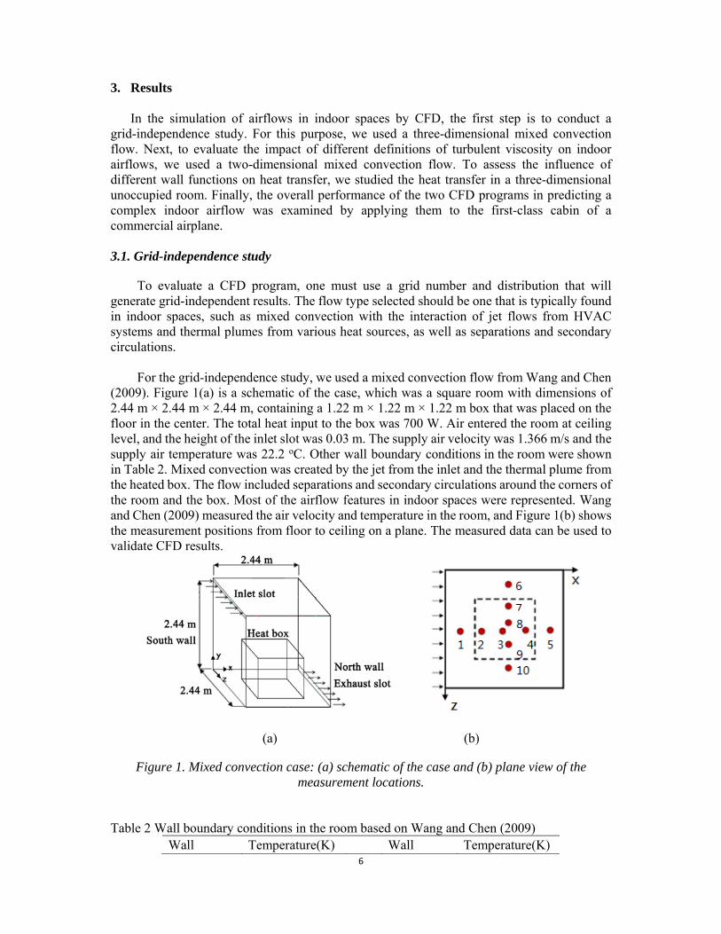
For the grid-independence study, we used a mixed convection flow from Wang and Chen

(2009). Figure 1(a) is a schematic of the case, which was a square room with dimensions of 2.44 m × 2.44 m × 2.44 m, containing a 1.22 m × 1.22 m × 1.22 m box that was placed on the floor in the center. The total heat input to the box was 700 W. Air entered the room at ceiling level, and the height of the inlet slot was 0.03 m. The supply air velocity was 1.366 m/s and the supply air temperature was 22.2 oC. Other wall boundary conditions in the room were shown in Table 2. Mixed convection was created by the jet from the inlet and the thermal plume from the heated box. The flow included separations and secondary circulations around the corners of the room and the box. Most of the airflow features in indoor spaces were represented. Wang and Chen (2009) measured the air velocity and temperature in the room, and Figure 1(b) shows the measurement positions from floor to ceiling on a plane. The measured data can be used to validate CFD results.

(a) (b)

Figure 1. Mixed convection case: (a) schematic of the case and (b) plane view of the measurement locations.

Table 2 Wall boundary conditions in the room based on Wang and Chen (2009)

Wall Temperature(K) Wall Temperature(K)

 

7  

Ceiling 299.09 Floor 303.3 North 300.16 South 300.47 West 300.9 East 301.03

In the grid independence study, we used the same hexahedral mesh for both programs. We

started with 20 cells in each direction and doubled the cell number progressively to 40, 80, and 160. As shown in Figure 2, the air velocity profile at a typical position, such as position 6, is the same with either 80 or 160 cells, which means 80 cells are sufficiently fine for this case. We used the same grid number in both programs to achieve the grid independent results. The two sets of numerical results also have similar accuracy in comparison with the experimental data at this position.

(a) (b) Figure 2. U-velocity profile at position 6 simulated by (a) STAR-CCM+ and (b) ANSYS Fluent with 20, 40, 80, and 160 cells in each direction, and comparison of the calculated results with

measured data from Wang and Chen (2009).

Although position 6 is representative, a more quantitative parameter is desirable for comparison with the experimental data and determination of grid independence. This investigation selected the normalized root mean square error (NRMSE), which is defined as:

2

1

max min

/n

iP i M i n

NRMSEM M

(15)

where P(i) and M(i) are the calculated and measured values, respectively, at location I,, and Mmax and Mmin are the maximum and minimum values, respectively, found in the experimental data.

Table 3 shows the NRMSE obtained by STAR-CCM+ and ANSYS Fluent with different cell numbers. The results confirm quantitatively that the solution was grid independent with 80 or more grid cells in each direction, because the NRMSE did not change with a further increase in cell number. The results shown in the table also indicate that the two programs can calculate

 

8  

the air distribution with high accuracy. Table 3. NRMSE for air temperature, air velocity, and turbulent kinetic energy with different grid numbers for STAR-CCM+ and ANSYS Fluent

Air temperature Air velocity Turbulent

kinetic energy Cell number STAR-

CCM+ ANSYS Fluent

STAR- CCM+

ANSYSFluent

STAR- CCM+

ANSYS Fluent

20 × 20 × 20 0.10 0.10 0.10 0.10 0.18 0.18 40 × 40 × 40 0.09 0.09 0.10 0.12 0.13 0.15 80 × 80 × 80 0.09 0.09 0.11 0.11 0.13 0.13

160 × 160 × 160 0.09 0.09 0.11 0.11 0.13 0.13 3.2. Impact of turbulence viscosity on air distribution

Next, we studied the effects of the different turbulence viscosity calculation methods in STAR-CCM+ and ANSYS Fluent, on the prediction of indoor airflow by these programs. For this purpose, we used the case of two-dimensional mixed convection with detailed experimental data from Blay et al. (1992). The flow was turbulent in the entire flow domain, and the experimental data was of high quality. We examined the impact of turbulence viscosity on the air distribution in terms of the resultant air velocity, temperature, and turbulence distributions.

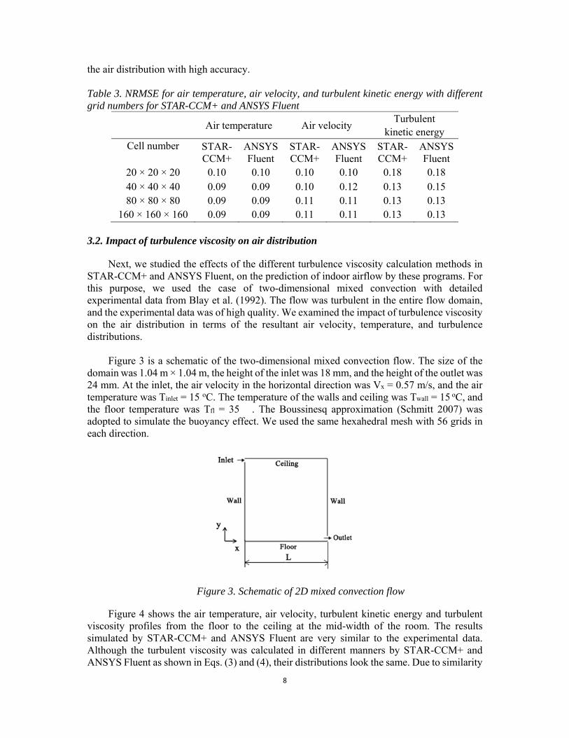
Figure 3 is a schematic of the two-dimensional mixed convection flow. The size of the

domain was 1.04 m × 1.04 m, the height of the inlet was 18 mm, and the height of the outlet was 24 mm. At the inlet, the air velocity in the horizontal direction was Vx = 0.57 m/s, and the air temperature was Tinlet = 15 oC. The temperature of the walls and ceiling was Twall = 15 oC, and the floor temperature was Tfl = 35 �. The Boussinesq approximation (Schmitt 2007) was adopted to simulate the buoyancy effect. We used the same hexahedral mesh with 56 grids in each direction.

Figure 3. Schematic of 2D mixed convection flow

Figure 4 shows the air temperature, air velocity, turbulent kinetic energy and turbulent viscosity profiles from the floor to the ceiling at the mid-width of the room. The results simulated by STAR-CCM+ and ANSYS Fluent are very similar to the experimental data. Although the turbulent viscosity was calculated in different manners by STAR-CCM+ and ANSYS Fluent as shown in Eqs. (3) and (4), their distributions look the same. Due to similarity

 

9  

on the turbulence viscosity distributions, their impacts on the air velocity and air temperature were the same in this case. As pointed out in Section 2.1, T = k/ε is valid in regions away from a wall. Near the wall, T ≠ k/ε, and thus one can see small differences in air velocity and turbulence kinetic energy near the wall as shown in Figure 4(b) and (c).

(a) (b)

(c) (d)

Figure 4. Comparison of (a) air temperature, (b) air velocity, (c) turbulent kinetic energy, and (d) turbulent viscosity at the mid-width of the cavity computed for different turbulence viscosities, with the experimental data from Blay et al. (1992).

We also used the case of three-dimensional mixed convection shown in Figure 2 to assess the impact of turbulent viscosity calculations on the airflow. The results agree with the experimental data. The accuracy was similar to those illustrated in Figure 4 for the two-dimensional case, although there were fewer measurement points near the walls. The two cases are complementary in showing the agreement with the corresponding experimental data.

 

10  

Because the case in Figure 2 was three dimensional, the airflow was more complex in Figure 4. Thus, the predictions had larger differences from the experimental data than did the predictions in Figure 4. 3.3. Impact of the wall function for temperature on heat transfer

STAR-CCM+ and ANSYS Fluent use different wall functions. The wall function for temperature is responsible for predicting heat transfer on walls. Fisher (1995) measured heat transfer in an unoccupied full-scale room, and we have used his experimental data to examine the wall functions in the two programs.

The room studied by Fisher (1995) had dimensions of 4.57 m × 2.74 m × 2.74 m and a horizontal inlet, as shown in Figure 5. The air temperature from the inlet was 15 oC, and there were two test cases with volumetric air flow rates of 6 ACH and 3.1 ACH, respectively. The airflow rate of 3.1 ACH is typical for mechanical ventilation in a room, but in the tests, it had a large experimental uncertainty.

Figure 5. Schematic of the unoccupied room

All the grids were created with appropriate y+ values according to the corresponding wall

functions. Namely, the finest grid had y+ < 1 for all y+ wall treatment in STAR-CCM+ and for the enhanced wall treatment in ANSYS Fluent. The coarsest grid had y+ > 30 for the high y+ wall treatment in STAR-CCM+ and for the standard wall function in ANSYS Fluent. The moderate grid was used for the all y+ wall treatment in STAR-CCM+ and the scalable wall function in ANSYS Fluent.

Figure 6 depicts the heat fluxes that were calculated for the surfaces concerned, along with the corresponding experimental data. Note that in the experiment the vertical walls were divided into three sections according to height. The calculated heat flux in the upper part of the room was generally lower than the experimentally measured heat flux, and in the lower part of the room it was higher than the measured heat flux. The measured convective heat transfer coefficient is related to the enclosure turbulent Reynolds number (Fisher 1995):

0.8~

hLNu Re

K (20)

where h is the convective heat transfer coefficient, K the thermal conductivity of the fluid, L the characteristic length, and Nu the Nusselt number.

In the upper part of the room, the local Reynolds number was very small, and the low turbulence caused the heat transfer coefficient to be low. Because of the weak convection, all the wall functions performed well. In the lower part of the room, the air was turbulent and the

 

11  

Reynolds number was larger. A higher heat transfer coefficient was observed. The enhanced wall treatment used in ANSYS Fluent calculated a heat transfer coefficient that was closest to the experimental data, compared with using other wall treatments. With the all y+ wall treatment used in STAR-CCM+, the fine grid (y+ < 1) was better than that with the coarse grid (y+ > 1). When a moderate grid was used (1 < y+ < 30), the all y+ treatment in STAR-CCM+ and the scalable wall function in ANSYS Fluent performed similarly for the two cases. Note that for these two cases, when the high y+ wall treatment was used in STAR-CCM+ and the standard wall function in ANSYS Fluent, the moderate grid did not provide significantly better results than the coarsest grid (y+ > 30).

Table 4 shows the grid numbers used for the simulations. The finer the grid was, the more computing time was required. The difference in computing time between the finest and coarsest grid numbers was one order of magnitude, while the calculated heat transfer coefficients were not much better with the finer grid. For a complex indoor space with many heat transfer surfaces, the use of a coarse grid number may be preferable.

(a) (b)

Figure 6. Comparison of simulated and measured heat fluxes on the room surfaces (where the

experimental data is from Fisher (1995)): (a) 6 ACH and (b) 3.1 ACH Table 4. Grid number and computing times with different wall functions and air flow rates of 3 ACH

 

12  

y+ y+ < 1 1 < y+ < 30 y+ > 30

Wall function

All y+ wall treatment in

STAR- CCM+

Enhanced wall

treatment in ANSYS Fluent

All y+ wall treatment in STAR-

CCM+

Scalable wall

function in ANSYS Fluent

High y+ wall

treatment in STAR-

CCM+

Standard wall

function in

ANSYS Fluent

Grid number

70 × 65 × 56 60 × 50 × 46 50 × 32 × 29

Computing time (min)

88.7 65.6 31.9 23.4 7.8 7.7

3.4. Accuracy of the two CFD programs in simulating complex indoor airflows

The previous cases were all rather simple in geometry. This investigation also used the first-class cabin of an MD-82 commercial airplane (Liu et al. 2012) to assess the accuracy of the two CFD programs in simulating indoor airflows with complex geometry and with multiple jets and heat sources. As shown in Figure 7, the first-class cabin was 3.28 m long, 2.91 m wide, and 2.04 m high with 12 seats in three rows. There were three and a half sections of air supply diffusers on each side. Each diffuser section had 280 linear slots that were each 22 mm long and 3 mm wide. The air was exhausted from outlets on each side of the wall near the floor. According to experimental measurements (Liu et al. 2012), the air velocity and air temperature varied from slot to slot in the cabin. To set the boundary conditions for the air supply inlets, we applied user-defined functions. The two CFD programs provided user-defined functions that were sufficiently good for this purpose, although ANSYS Fluent was more user-friendly than STAR-CCM+ in our experience.

Figure 7. The first-class cabin of an MD-82 commercial airplane.

Figure 8 compares the simulated airflow patterns with the experimental data measured by

ultra-sonic anemometers at a cross section through the second row of the cabin. Both CFD programs were able to simulate the airflow pattern, but none of the results agree well with the experimental data. For such a complex flow, in our experience, it is difficult to obtain good agreement, even with more advanced simulation techniques (Liu et al. 2013).

 

13  

Figure 8. Comparison of the airflow patterns calculated by STAR-CCM+ and ANSYS Fluent

with the experimental data at a cross section through the second row of the cabin.

In order to quantitatively assess the performance of the two CFD programs, this investigation defined absolute error and relative error as

Absolute Error = P i M i (15)

Relative Error =

P i M i

M i

(16)

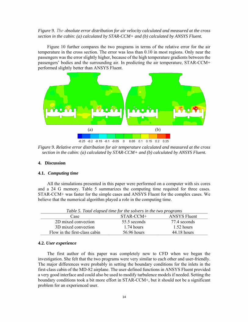
where P(i) is the air velocity or temperature calculated by STAR-CCM+ or ANSYS Fluent and M(i) the measured value. As shown in Figure 9, the two CFD programs had an absolute error of less than 0.05 for most regions in the cross-section. In the regions near the right inlet and close to the floor, the errors were larger. Near either inlet, the velocity gradient was very large, and a small deviation in the measuring position could have caused a large error. Furthermore, when the ultrasonic anemometers were positioned during the experiment, it was difficult to access the area near the floor. Of course, the errors may not be fully associated with the positioning of the instruments. Other factors, such as turbulence models and numerical algorithms, could also have contributed to the differences. If the goal of our CFD study had been to improve the thermal comfort level in the cabin, the error would be considered as small. Figure 9 also indicates that ANSYS Fluent performed slightly better than STAR-CCM+ in simulating the air velocity.

(a) (b)

 

14  

Figure 9. The absolute error distribution for air velocity calculated and measured at the cross section in the cabin: (a) calculated by STAR-CCM+ and (b) calculated by ANSYS Fluent.

Figure 10 further compares the two programs in terms of the relative error for the air temperature in the cross section. The error was less than 0.10 in most regions. Only near the passengers was the error slightly higher, because of the high temperature gradients between the passengers’ bodies and the surrounding air. In predicting the air temperature, STAR-CCM+ performed slightly better than ANSYS Fluent.

(a) (b)

Figure 9. Relative error distribution for air temperature calculated and measured at the cross

section in the cabin: (a) calculated by STAR-CCM+ and (b) calculated by ANSYS Fluent.

4. Discussion

4.1. Computing time

All the simulations presented in this paper were performed on a computer with six cores and a 24 G memory. Table 5 summarizes the computing time required for three cases. STAR-CCM+ was faster for the simple cases and ANSYS Fluent for the complex cases. We believe that the numerical algorithm played a role in the computing time.

Table 5. Total elapsed time for the solvers in the two programs Case STAR-CCM+ ANSYS Fluent

2D mixed convection 55.5 seconds 77.4 seconds 3D mixed convection 1.74 hours 1.52 hours

Flow in the first-class cabin 56.96 hours 44.18 hours 4.2. User experience

The first author of this paper was completely new to CFD when we began the investigation. She felt that the two programs were very similar to each other and user-friendly. The major differences were probably in setting the boundary conditions for the inlets in the first-class cabin of the MD-82 airplane. The user-defined functions in ANSYS Fluent provided a very good interface and could also be used to modify turbulence models if needed. Setting the boundary conditions took a bit more effort in STAR-CCM+, but it should not be a significant problem for an experienced user.

 

15  

5. Conclusion

This study used STAR-CCM+ and ANSYS Fluent to simulate several indoor airflow problems with the same mesh and boundary conditions and compared the simulated results with each other and with experimental data. The investigation led to the following conclusions:

(1) The two CFD programs reached grid-independent solutions with the same mesh size, and

the accuracy of the predicted results was similar. (2) Although the programs calculated the turbulent viscosity differently, the resultant

distributions of air velocity, air temperature, and turbulence kinetic energy were nearly the same.

(3) The two programs used different wall functions for temperature. The results obtained by the two programs showed that the finer the grid, the more accurate the heat transfer coefficient. The enhanced wall treatment used in ANSYS Fluent calculated a heat transfer coefficient that was in good agreement with the experimental data.

(4) The CFD programs calculated complex airflows with similar accuracy. ANSYS Fluent performed slightly better, and its user-defined functions were more user-friendly.

Acknowledgements The research presented in this paper was financially supported by the national key project of the Ministry of Science and Technology, China, on “Green Buildings and Building Industrialization” through Grant No. 2016YFC0700500. References Ali AA (2012) CFD Investigation of indoor air distribution in marine applications. European

Journal of Scientific Research, 88:196-208. ANSYS (2016) ANSYS Fluent 17.0 Documentation. ANSYS, Inc., Lebanon, NH.

Blay D, Mergui S, Niculae C (1992) Confined turbulent mixed convection in the presence of a horizontal buoyant wall jet. ASME –HTD 213(1992):65-72.

Cablé A, Michaux G, Inard C (2012) Addressing summer comfort in low-energy housing using the air vector: A numerical and experimental study. In: Proceedings of the 33rd AIVC Conference, Copenhagen, Denmark, pp. 10-11.

CD-adapco (2016) STAR-CCM+ 11.0 User Guide. CD-adapco, Inc. Chen C, Liu W, Li F, Lin C-H, Liu J, Pei J, Chen Q (2013) A hybrid model for investigating

transient particle transport in enclosed environments. Building and Environment 62:45-54.

Chen Q, Srebric J (2002) A procedure for verification, validation, and reporting of indoor environment CFD analyses. HVAC & R Research 8(2): 201-216.

Chen Q (1995) Comparison of different k-ε models for indoor air flow computations. Numerical Heat Transfer, Part B: Fundamentals, 28(3): 353-369.

Chen Q (2009) Ventilation performance prediction for buildings: A method overview and recent applications. Building and Environment 44(4): 848-858.

Craft TJ, Gerasimov AV, Iacovides H, Launder BE (2002) Progress in the generalization of wall-function treatments. Int J Heat Fluid Flow, 23:148-60.

Durbin PA (1991) Near-wall turbulence closure modeling without damping functions. Theoretical and Computational Fluid Dynamics, 3:1-13.

Fisher DE (1995) An experimental investigation of mixed convection heat transfer in a rectangular enclosure. Ph.D. thesis, Department of Mechanical and Industrial

 

16  

Engineering, University of Illinois at Urbana-Champaign, IL. Fiser J, Jícha M (2013) Impact of air distribution system on quality of ventilation in small

aircraft cabin. Building and Environment, 69:171-182. Kiš P, Herwig H (2012) The near wall physics and wall functions for turbulent natural

convection. Int J Heat Mass Transf, 55: 2625-35. Kuznik F, Brau J, Rusaouen G (2007) RSM model for the prediction of heat and mass transfer

in a ventilated room. In: Proceeding of Building Simulation 2007, pp. 919-926. Ladeinde F, Nearon M (1997) CFD applications in the HVAC&R industry. ASHRAE Journal

39(1): 44. Launder BE and. Spalding DB (1974) The numerical computation of turbulent flows. Comput

Meth Appl Mech Eng 3: 269-89. Li N (2015) Comparison between three different CFD software and numerical simulation of an

ambulance hall. KTH School of Industrial Engineering and Management Energy Technology, Division of Energy Technology, Sweden.

Liu S, Xu L, Chao J, Shen C, Liu J, Sun H, Xiao S, Nan G (2013) Thermal environment around passengers in an aircraft cabin. HVAC&R Res, 19:627-634.

Liu W, Lin C-H, Liu J, Chen Q (2011) Simplifying geometry of an airliner cabin for CFD simulations. In: Proceedings of the 12th International Conference on Indoor Air Quality and Climate. Austin, TX, a118-23.

Liu W, Mazumdar S, Zhang Z, Poussou SB, Liu J, Lin SH, Chen Q (2012) State-of-the-art methods for studying air distributions in commercial airliner cabins. Building and Environment 47:5-12.

Liu W, Wen J, Chao J, Yin W, Shen C, Lai D, Lin C-H, Liu J, Sun H, Chen Q (2012) Accurate and high-resolution boundary conditions and flow fields in the first-class cabin of an MD-82 commercial airliner. Atmospheric Environment, 56: 33-44.

Liu W, Wen J, Lin C-H, Liu J, Long Z, Chen Q (2013) Evaluation of various categories of turbulence models for predicting air distribution in an airliner cabin. Building and Environment 65:118-131.

Nielsen PV (1976) Flow in air conditioned rooms. Ph.D. thesis, Technical University of Denmark.

Patankar SV, Spalding DB (1972) A calculation procedure for heat, mass and momentum transfer in three-dimensional parabolic flows. International Journal of Heat and Mass Transfer, 15(10):1787-1806.

Ružić D (2015) Influence of the ventilation system setting in the passenger car on the local thermal sensation of a driver. J. of Thermal Science and Technology 35(1): 125-134.

Stephen BP (2000) Turbulent Flows. 1st Edition, Cambridge University Press, Cambridge, United Kingdom.

Schmitt FG (2007) About Boussinesq’s turbulent viscosity hypothesis: Historical remarks and a direct evaluation of its validity. Comptes Rendus Mécanique 335(9-10): 617-627.

Srebric J, Chen Q (2002) An example of verification, validation, and reporting of indoor environment CFD analyses (RP-1133). ASHRAE Transactions 108(2): 185-194.

Wang M, Chen Q (2009) Assessment of various turbulence models for transitional flows in an enclosed environment (RP1271). HVAC&R Research, 15(6): 1099-1119.

Wang M, Lin C-H, Chen Q (2011) Determination of particle deposition in enclosed spaces by Detached Eddy Simulation with the Lagrangian method. Atmospheric Environment 45: 5376-5384.

Yuan X, Chen Q, Glicksman LR, Hu Y, Yang X (1999) Measurements and computations of room airflow with displacement ventilation. ASHRAE Transactions, 105: 340-352.

Zhang T, Lee KS, Chen Q (2009) A simplified approach to describe complex diffusers in displacement ventilation for CFD simulations. Indoor Air 19(3): 255-267.

 

17  

Zhang T, Zhou H, Wang S (2013) An adjustment to the standard temperature wall function for CFD modeling of indoor convective heat transfer. Building and Environment 68:159-169.