comparison of the seasonal and interannual variability of ... · comparison of the seasonal and...
TRANSCRIPT
JOURNAL OF GEOPHYSICAL RESEARCH, VOL. 99, NO. C4, PAGES 7355-7370, APRIL 15, 1994
Comparison of the seasonal and interannual variability of phytoplankton pigment concentrations in the Peru and California Current systems
A. C. Thomas and F. Huang Atlantic Centre for Remote Sensing of the Oceans, Halifax, Nova Scotia, Canada
P. T. Strub and C. James
College of Oceanic and Atmospheric Sciences, Oregon State University, Corvallis
Abstract. Monthly composite images from the global coastal zone color scanner (CZCS) data set are used to provide an initial illustration and comparison of seasonal and interannual variability of phytoplankton pigment concentration along the western coasts of South and North America in the Peru Current system (PCS) and California Current system (CCS). The analysis utilizes the entire time series of available data (November 1978 to June 1986) to form a mean annual cycle and an index of interannual variability for a series of both latitudinal and cross-shelf regions within each current system. Within 100 km of the coast, the strongest seasonal cycles in the CCS are in two regions, one between 34 ø and 45øN and the second between 24 ø and 29øN, each with maximum concentrations (>3.0 mg m -3) in May-June. Weaker seasonal variability is present north of 45øN and in the Southern California Bight region (32øN). Within the PCS, in the same 100-km-wide coastal region, highest (>45øS) and lowest (<20øS) latitude regions have a similar seasonal cycle with maximum concentrations (> 1.5 mg m -3) during the austral spring, summer, and fall, matching that evident throughout the CCS. Between these regions, off northern and central Chile, the seasonal maximum occurs during July-August (austral winter), contrary to the influence of upwelling favorable winds. Within the CCS, the dominant feature of interannual variability in the 8-year time series is a strong negative concentration anomaly in 1983, an E1 Nifio year. The relative value of this negative anomaly is strongest off central California and is followed by an even stronger negative anomaly in 1984 off Baja California. In the PCS, strong negative anomalies during the 1982-1983 E1 Nifio period are evident only off the Peruvian coast and are evident there only in the regions 100 km or more from the coast. Although negative anomalies associated with the E1 Nifio were not present at higher latitudes (more than approximately 20øS) in the PCS, the extremely sparse sampling weakens our confidence in the results of the interannual analysis in this region. An upper estimate of the systematic winter bias remaining in the global CZCS data after reprocessing with the multiple scattering algorithm is given in the appendix.
1. Introduction
A major oceanographic characteristic of eastern boundary currents (EBCs) is the presence of recurring wind-driven coastal upwelling. Physical forcing introduces nutrient-rich subsurface water into the upper water column, resulting in increased phytoplankton production and concentrations. Large, multidisciplinary and multiyear programs such as Coastal Upwelling Ecosystems Analysis (CUEA) and Coop- erative Investigation of the Northern Part of the Eastern Central Atlantic (CINECA) demonstrated the strong tempo- ral and spatial variability of both physical dynamics and biological patterns in EBCs. More recently, programs such as the Coastal Ocean Dynamics Experiment (CODE), Orga- nization of Persistent Upwelling Structures (OPUS) and
Copyright 1994 by the American Geophysical Union.
Paper number 93JC02146. 0148-0227/94/93JC-02146505.00
Coastal Transition Zone programs have provided details of both physical and physiological processes on relatively localized space and time scales.
Previous comparisons between the dynamics of different eastern boundary currents [e.g., Smith, 1981; Schulz, 1982; Minas et al., 1986] which relied on in situ data were, by necessity, restricted in the time and space scales they could address and rarely had access to temporally coincident data from the different regions. The repetitive, large-scale synop- tic views offered by satellite observations are well suited for estimating the temporal and spatial scales of variability of near-surface oceanographic characteristics. Over the last decade, satellite images of ocean color from the coastal zone color scanner (CZCS) have revealed many of the larger-scale time and space features of biological variability of the California Current system (CCS) [Abbott and Zion, 1987; Pelaez and McGowan, 1986; Smith et al., 1988] and some details of structure within the Peru Current system (PCS)
7355
7356 THOMAS ET AL ß PERU AND CALIFORNIA CURRENT PIGMENT VARIABILITY
[e.g., Uribe and Neshyba, 1983; Espinoza et al., 1983]. Substantially fewer CZCS data were collected over the PCS. Sufficient images are available, however, to obtain a first approximation of the major seasonal features that are evi- dent in the available satellite ocean color data. Although biased by missing data toward certain years and months, they allow a general comparison of the larger-scale temporal and spatial variability of phytoplankton biomass in these two Pacific eastern boundary currents.
In this paper we present and compare the mean seasonal and interannual variability of phytoplankton pigment con- centrations along the west coasts of North and South Amer- ica in the Peru and the California Current systems. The time series of CZCS data includes 1982-1983, a period with a particularly strong E1 Nifio event [Cane, 1983; Barber and Chavez, 1986]. The analysis is offered as a general summary and synthesis of the larger-scale temporal and spatial fea- tures which can be deduced from the available CZCS data, flawed though that data set may be by poor sampling and potential bias. A more complete analysis of features on these time and space scales awaits the arrival of additional and hopefully more complete data from future color sensors, such as the sea-viewing wide-field sensor (Sea WiFS), sup- ported by in situ measurements.
Major features of the temporal variability in the California Current have previously been shown by Pelaez and McGowan [1986] and Thomas and Strub [1989, 1990] and compared to wind forcing by $trub et al. [1990]. A detailed description and analysis will not be repeated here. However, a recalculation of this variability in the CCS, warranted by the recent availability of the complete, global, reprocessed CZCS data set [Feldman et al., 1989], is made and pre- sented. These data were processed utilizing a multiple scat- tering algorithm in the atmospheric correction [Gordon et al., 1988], which reduces the errors caused by large solar zenith angles (high latitudes in winter months). In section 2 we summarize characteristics of the CZCS data and details
of the analysis methods. In section 3 we present the mean seasonal variability in the two EBCs and an analysis of interannual variability in the PCS and CCS over the 8-year extent of the CZCS data set. A comparison and discussion of patterns evident in the two EBCs is made in section 4, and a summary and conclusions follow in section 5. The appendix presents an empirical estimate of magnitude of the system- atic errors which might remain in the global CZCS data set owing to uncorrected atmospheric scattering at high lati- tudes in winter.
2. Data and Methods
The ocean pigment concentration measurements pre- sented here are from the coastal zone color scanner instru- ment aboard the Nimbus 7 satellite. The entire CZCS data
set has been reprocessed [Feldman et al., 1989] using a standard epsilon value and a multiple Rayleigh scattering algorithm in the atmospheric correction. One of the products of this reprocessing is a set of global fields of pigment concentration with a spatial resolution of 20 km, composited within calendar months. This image set was subsampled to provide two time series of 92 monthly images each, extend- ing over the entire CZCS lifetime, from November 1978 to June 1986. One series covers the Peru Current region from 6 ø to 51øS, and the second covers the California Current region from 21 ø to 48øN.
Gordon et al. [1983a] estimated the accuracy of the CZCS-derived pigment measurements to be log(chlorophyll) --.0.5 (i.e., within a factor of 2 in concentration). A compar- ison of CZCS data with ship measurements off southern California [Smith et al., 1988] showed the satellite data to be ---40% within the chlorophyll concentration range 0.05-10.0 mg m -3. Although the multiple-scattering algorithm used in processing the global data set improves the concentration estimates, especially at higher latitudes during winter months [Gordon and Castano, 1987; Gordon et al., 1988], a systematic bias may still be present. This bias, as well as other systematic and random errors associated with the CZCS data set, is discussed in more detail by Strub et al. [1990] and is not repeated here. An upper estimate of the magnitude of the possible winter bias in the data is given in the appendix. Efforts were made in the reprocessing of the data set [Feldman et al., 1989] to account for sensor degra- dation over the life of the sensor [Gordon et al., 1983b; Mueller, 1985].
The mean seasonal cycle in pigment concentration over the entire latitudinal extent of the PCS and the CCS was
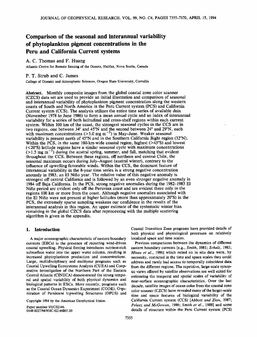
calculated. An overall mean image for each calendar month was formed by compositing all available images for a given month to form a 12-month series. These images are used to provide a qualitative description of spatial and temporal patterns over the year as well as regional differences within each EBC. Subsampling each of the mean monthly images by averaging within 100 x 100 km boxes oriented by the coast allows a quantitative analysis of these seasonal pat- terns and aids in filling regions of missing data due to clouds. The location of these boxes is shown in Figures la and lb. As with any data set, quantitative interpretation is subject to the errors and bias of the measurements (outlined above). In the vicinity of the highly complex coastline off southern Chile, a smoothed coastline oriented along the western side of the islands was used. Despite these spatial and temporal averaging procedures, some regions of the PCS still had missing data in some months. Missing data within a box in any month were supplied by spatially averaging the concen- trations from the boxes equidistant from the coast and immediately to the north and south for the same month. Total missing data supplied in this manner were less than 5% of the total matrix of 1836 data points (12 months x 3 offshore zones x 51 alongshore boxes).
Previous analyses of interannual variability in the Califor- nia Current using CZCS data [Pelaez and McGowan, 1986; Thomas and Strub, 1989, 1990; Strub et al., 1990] have shown that the coverage is generally sufficient to resolve features on time scales of a month or less. The CZCS data
set for the Peru Current is much less complete. To produce a time series allowing examination of interannual variability of the PCS over the lifetime of the CZCS, large-scale temporal and spatial averaging is necessary. This averages over gaps in the data set due to clouds and/or lack of collection effort but obviously reduces the amplitude of shorter time scale events. To accomplish this, 8-month composite images temporally centered on the midpoint of summer in each hemisphere were formed within each year of data coverage. For the California Current, the 8-month summer composite image in each year is of months March through October. For the Peru Current, the 8-month com- posite image was formed from the months September through April. The resultant image time series extends over
THOMAS ET AL.' PERU AND CALIFORNIA CURRENT PIGMENT VARIABILITY 7357
I [ I
ClFIC NORTHWEST REGION 45N
40N
- ' ..... 35N 1 SOUTHERN CALIFORNIA BIGHT•
- 30N J
_ BAJA CALIFORN• REGION
125W 120W 115W 110•
] j[ ] I I
NORTHERN CHILE till ZSS 4 _ •NTRAL C•
,
- SOUTHERN CHILE -'
Figure 1. (a) The California Current system and (b) the Peru Current system study areas showing the regions within which image data were spatially averaged to extract seasonal and interannual variability. The solid lines show the three 100-km-wide strips parallel to the coasts extending offshore and the extents of four regions used to illustrate interannual variability. The dashed lines indicate the system of 100 x 100 km boxes used to spatially average the image data for presentation of mean seasonal cycles.
8 years in each study region. For the CCS, the 1986 composite is from March to June, and for the PCS the 1978-1979 composite is from November to April.
Quantitative analysis of interannual variability in pigment concentration was carried out by sub sampling and spatially averaging within these 8-month composite images to derive mean concentrations. These were calculated over each of
four latitudinal zones extending 400 km or more alongshore. An annual anomaly was formed by subtracting the overall mean concentration (the mean of the 8-month period over all 8 years) for each zone from the concentrations found in each year. The sample zones are oriented by the coastline in the same manner as the smaller boxes used above for the
seasonal cycle. To illustrate cross-shelf differences in inter- annual variability, each latitudinal zone was subdivided into three 100-km-wide areas, and a separate mean was calcu- lated for each. This resulted in a time series for each
latitudinal zone and each of the three offshore bands (0-100, 100-200, and 200-300 km) shown in Figures l a and lb.
3. Results
3.1. Seasonal Cycles
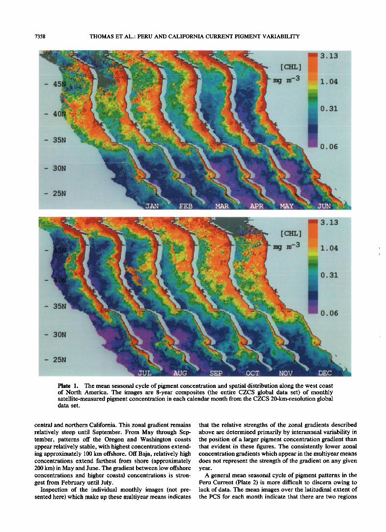
The multiyear means of pigment concentration for each month of the calendar year are shown in Plates 1 and 2 for the California Current and Peru Current regions, respec- tively. Spatial resolution in these composites is the 20 x 20 km pixel dimensions of the original global data set. A presentation of the number of years (samples) which make up each pixel in each monthly mean is given in Figures 2 and 3. In general, pixel values within the monthly composite images of the CCS are from 5 or more years of data. As was previously stated, Figure 3 shows that coverage of the PCS
is substantially less. In many months, some areas of the PCS are represented by only 2 to 3 years of data, and a few areas in some months remain completely unsampled. Lack of coverage is most severe during months of austral winter (June, July). These images are composed of data from only 1-2 years.
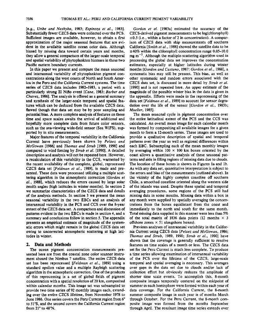
-3 Plate 1 shows that concentrations greater than 2.0 mg m
are found within approximately 40 km of the coast through- out the year and throughout the latitudinal range of the CCS study area. High concentrations (>1.0 mg m -3) extend farthest from shore off northern and central California (ap- proximately 34 ø to 43øN) and to a lesser degree off Baja California (south of 30øN). Higher pigment concentrations remain most closely associated with the coast throughout the year in the California Bight and southern California regions. High concentrations (> 1.0 mg m -3) appear to extend far- thest from shore in November, December, and January, forming a diffuse pattern off northern and central California with no strong zonal gradients. Although these values from late fall and early winter may continue to be contaminated by incompletely removed atmospheric effects [Strub et al., 1990], in the appendix we estimate the maximum magnitude of such errors to be less than 0.15 mg m -3 south of 40øN, rising to 0.4 mg m -3 or less at 48øN. In February these highest concentrations are closer to shore in this region, but in March they appear to extend up to 700 km offshore again, as shown by Thomas and $trub [1989]. In April the diffuse pattern of offshore higher concentrations appears to consol- idate closer to the coast. By May the highest concentrations are within approximately 200 km of the coast, and a rela- tively sharp frontal gradient separating higher pigment con- centrations from very low offshore concentrations is estab- lished. In June this gradient takes on a scalloped shape off
7358 THOMAS ET AL.' PERU AND CALIFORNIA CURRENT PIGMENT VARIABILITY
- 45N
- 40I - ß
- 35N
- 30N
- 25N
•.. [CHL] ß
.
" mg m -3
•IAN FEB MAR APR MAY
[CHL]
mg m-3
3.13
1.04
0.31
0.06
JUN
3.13
1.04
0.31
- 35N
- 30N
ø•"-'•' "k, O. 06
- 25N
JUL AUG SEP OCT NOV DEC
Plate 1. The mean seasonal cycle of pigment concentration and spatial distribution along the west coast of North America. The images are 8-year composites (the entire CZCS global data set) of monthly satellite-measured pigment concentration in each calendar month from the CZCS 20-km-resolution global data set.
central and northern California. This zonal gradient remains relatively steep until September. From May through Sep- tember, patterns off the Oregon and Washington coasts appear relatively stable, with highest concentrations extend- ing approximately 100 km offshore. Off Baja, relatively high concentrations extend farthest from shore (approximately 200 km) in May and June. The gradient between low offshore concentrations and higher coastal concentrations is stron- gest from February until July.
Inspection of the individual monthly images (not pre- sented here) which make up these multiyear means indicates
that the relative strengths of the zonal gradients described above are determined primarily by interannual variability in the position of a larger pigment concentration gradient than that evident in these figures. The consistently lower zonal concentration gradients which appear in the multiyear means does not represent the strength of the gradient on any given year.
A general mean seasonal cycle of pigment patterns in the Peru Current (Plate 2) is more difficult to discern owing to lack of data. The mean images over the latitudinal extent of the PCS for each month indicate that there are two regions
THOMAS ET AL.: PERU AND CALIFORNIA CURRENT PIGMENT VARIABILITY 7359
•:-_::::-:-: -•-•<•:.:-.---.o•< .... - .................... • ::::-'.-:::::::::::8:::.?' ::::::::::::::::::::::::::::::::::::::::::::::::::::::::: ::::::::::::::::::::::::::::::::::::::::::::::::::::::::::::: ::::::::::::::::::::::::::::::::::::::::::::::::::::::: ...... ........
_• =:-----------:::.---•-- • :::::::::::::::::::::::::::::::::::::::::::::::::::::: ::::::::::::::::::::::::::::::::::::::::::::::::::::::::::: ::::::::::::::::::::::::::::::::::::::::::::::::::::::::::: :::::::::::::::::::::::::::::::::::::::::::::::::::::: ::::::::::::::::::
============================================================= .... ========================================================== .... ====================================================== .... ========================================================= .... ========================================================= .... ========================================================= .... .... . ...... ... ..... . ............. -....: ............ :.:.:.:.:-:.:.:.:.:.:.:.:.. '•::::::::: :::::::::::::::::::::::::::::::::::::::::::::: ============================================================ ===================== ::::::::5::::::::: ::::::::: ::::::. ============================================== :::::::::::..
============================================= =========================================================== ======================================================== .... ::::::::::::::::::::::::::::::::::::::::::::::::::::::: ============================================================== ... =======================================================
=================================================================== .--.:-:.:.:.:.:.:-:.:-:.:.:.:.:.:.:.:.:.:.:.:.:.:-:-:.:..... --.-.:.:.:.:.:.:.:.:.:.:.:.:.:.:.:.:.:.:.:.:.:.:.:.:.:.:.........:.:.:.:.:.:.:.:.:.:.:.:.:.:.:.:.:.:.:.:.:.:.:.:.:.:..... =============================================================== =========================================== ..::::::...:... .......................................................... ......................................_................... ....:.:.:.:.:.:.:...:.:.:.:.:.:.:.:.:.:.:.:.:.:.:.:.:.:.:... .......................................................... ..................................................
::::::::::::::::::::::::::::::::::::::::: ====================================== ====================================================== :::::::::::::::::::::::::::::::::::::::::::::::::::: ================================================ •:::.::::::'.
•::: :::::::'•:•:::::::::::::::::::::::::::::::::::::::: ========================================================= -::: ::::::::::::::::::::::::: ::::' ::::::::::::::: ::::::::::::: ::::::: ::::: ::: ::::' :'":'•i•::•:'.•:::::":•:: :: :: :":.: '•:::i::' -•'• ...-: ......
....... .:::::::::::::::::::::::::.•::::::::::::::::::•::::::::::.:.:.:.:.::::::•:::::::::::::::::::::•:•:•::::::::::::::::::::::::::.:::::.:.::::::::::::::::::::::::::::::::::•:::::::::::::::::::::::::..::......:::::::•::.::::::•:•:::•:::::::::::::::::::::::•::::::::::...:.:.....::::::•:::::::•:::::::::::•:•:•:::::::::::::::::•:::::::::..:.:.....::::::::::::::::::::::::::::::::::::::•:•::::::::::.:::::: .....
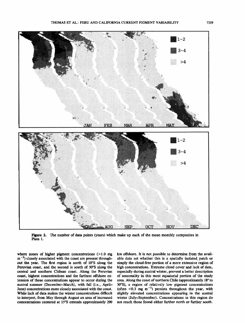
Figure 2. The number of data points (years) which make up each of the mean monthly composites in Plate 1.
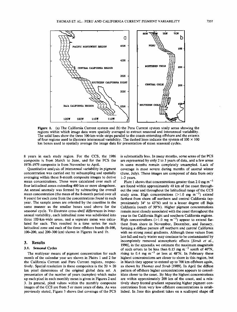
where zones of higher pigment concentrations (>1.0 mg m -3) closely associated with the coast are present through- out the year. The first region is north of 18øS along the Peruvian coast, and the second is south of 30øS along the central and southern Chilean coast. Along the Peruvian coast, highest concentrations and the farthest offshore ex- tension of these concentrations appear to occur during the austral summer (December-March), with fall (i.e., April- June) concentrations more closely associated with the coast. While lack of data makes the winter concentrations difficult
to interpret, from May through August an area of increased concentrations centered at 15øS extends approximately 200
km offshore. It is not possible to determine from the avail- able data set whether this is a spatially isolated patch or simply the cloud-free portion of a more extensive region of high concentrations. Extreme cloud cover and lack of data, especially during austral winter, prevent a better description of seasonality in this most equatorial portion of the study area. Along the coast of northern Chile (approximately 18 ø to 30øS), a region of relatively low pigment concentrations (often <0.3 mg m -3) persists throughout the year, with slightly elevated concentrations appearing in the austral winter (July-September). Concentrations in this region do not reach those found either farther north or farther south.
7360 THOMAS ET AL.' PERU AND CALIFORNIA CURRENT PIGMENT VARIABILITY
- 10S
- 20S
- 30S
- 40S
_ 50S JAN APR '•' MAY"'" .JUN
[CHL] -3
mc3m
lOS
- 20S
- 30S
- 40S
_ 50S UL • A .• SEP OCT ' NO
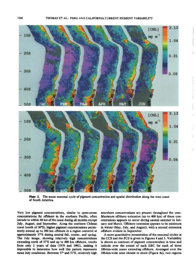
Plate 2. The mean seasonal cycle of pigment concentration and spatial distribution along the west coast of South America.
3.13
1.04
0.31
0.06
3.13
1.04
0.31
0.06
Very low pigment concentrations, similar to open-ocean concentrations far offshore in the southern Pacific, often intrude to within 40 km of the coast during all months except July, August, and September. Along the southern Chilean coast (south of 30øS), higher pigment concentrations persis- tently extend up to 200 km offshore in a region centered at approximately 37øS during austral fall, winter, and spring. The July image, showing relatively high concentrations extending north of 37øS and up to 400 km offshore, results from only 2 years of data (1979 and 1981), making it impossible to determine how well this pattern represents mean July conditions. Between 37 ø and 51øS, relatively high
nearshore concentrations are present throughout the year. Maximum offshore extension (up to 400 km) of these con- centrations appears to occur during austral summer in Jan- uary and March. Offshore extension appears to be minimum in winter (May, July, and August), with a second extension offshore evident in September.
A more quantitative presentation of the seasonal cycles in the CCS and the PCS is given in Figures 4 and 5. Variability is shown as contours of pigment concentration in time and latitude over the extent of each EBC for each of three
100-km-wide zones extending offshore. Averaged over the 100-km-'wide zone closest to shore (Figure 4a), two regions
THOMAS ET AL.: PERU AND CALIFORNIA CURRENT PIGMENT VARIABILITY 7361
l-2
ß '•-::::•;.-'--..-•ii: :'::.:':?-:•:..::- 7-•:':•.'• •,::::•i•:i:i•:ii::i•,:ii 3-4
ß :.:.::::::::::::.:
':'"i::•:i.:.•: .• i.•'"
....- .................. .
::::::::::::::::::::::::::::::::::::: .. ß
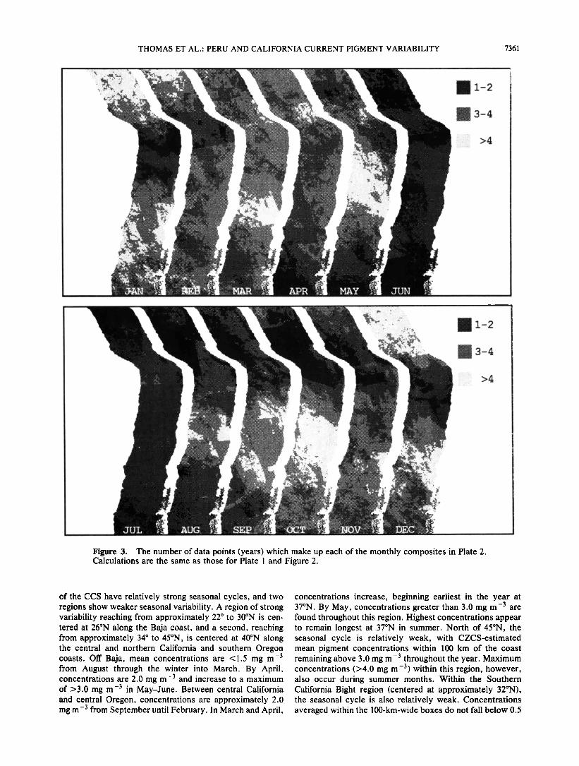
Figure 3. The number of data points (years) which make up each of the monthly composites in Plate 2. Calculations are the same as those for Plate I and Figure 2.
of the CCS have relatively strong seasonal cycles, and two regions show weaker seasonal variability. A region of strong variability reaching from approximately 22 ø to 30øN is cen- tered at 26øN along the Baja coast, and a second, reaching from approximately 34 ø to 45øN, is centered at 40øN along the central and northern California and southern Oregon
-3 coasts. Off Baja, mean concentrations are <1.5 mg m from August through the winter into March. By April, concentrations are 2.0 mg m -3 and increase to a maximum of >3.0 mg m -3 in May-June. Between central California and central Oregon, concentrations are approximately 2.0 mg m-3 from September until February. In March and April,
concentrations increase, beginning earliest in the year at 37øN. By May, concentrations greater than 3.0 mg m -3 are found throughout this region. Highest concentrations appear to remain longest at 37øN in summer. North of 45øN, the seasonal cycle is relatively weak, with CZCS-estimated mean pigment concentrations within 100 km of the coast remaining above 3.0 mg m -3 throughout the year. Maximum concentrations (>4.0 mg m -3) within this region, however, also occur during summer months. Within the Southern California Bight region (centered at approximately 32øN), the seasonal cycle is also relatively weak. Concentrations averaged within the 100-km-wide boxes do not fall below 0.5
7362 THOMAS ET AL.' PERU AND CALIFORNIA CURRENT PIGMENT VARIABILITY
44
.0 '
3O
NDJ FM AMJ J AS OND JF
(] 0 - 100 KM OFFSHORE
40
3[5 i -
•i 34 ' ' i . . 32 ;,;,,,,•. 5•. 5•
.
i
30 ,,
.
26
.
b •oo - •oo n• on, s•o•. c •oo - •oo • o•s•o•s
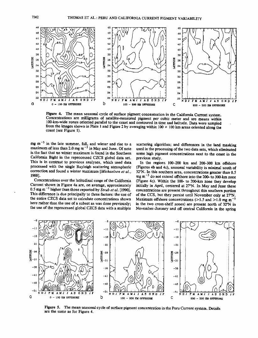
Figure 4. The mean seasonal cycle of surface pigment concentration in the California Current system. Concentrations are milligrams of satellite-measured pigment per cubic meter and are means within 100-km-wide zones oriented parallel to the coast and contoured in time and latitude. Data were sampled from the images shown in Plate 1 and Figure 2 by averaging within 100 x 100 km areas oriented along the coast (see Figure 1).
mg m -3 in the late summer, fall, and winter and rise to a maximum of less than 2.0 mg m-3 in May and June. Of note is the fact that no winter maximum is found in the Southern California Bight in the reprocessed CZCS global data set. This is in contrast to previous analyses, which used data processed with the single Rayleigh scattering atmospheric correction and found a winter maximum [Michaelsen et al., 1988].
Concentrations over the latitudinal range of the California Current shown in Figure 4a are, on average, approximately 0.5 mg m-3 higher than those reported by $trub et al. [ 1990]. This difference is due principally to three factors: the use of the entire CZCS data set to calculate concentrations shown here rather than the use of a subset as was done previously; the use of the reprocessed global CZCS data with a multiple
scattering algorithm; and differences in the land masking used in the processing of the two data sets, which eliminated some high pigment concentrations next to the coast in the previous study.
In the regions 100-200 km and 200-300 km offshore (Figures 4b and 4c), seasonal variability is minimal south of 32øN. In this southern area, concentrations greater than 0.5 mg m -3 do not extend offshore into the 200- to 300-km zone (Figure 4c). Within the 100- to 200-km zone they develop initially in April, centered at 27øN. In May and June these concentrations are present throughout this southern portion of the CCS, but they persist until November only at 27øN. Maximum offshore concentrations (> 1.5 and > 1.0 mg m -3 in the two cross-shelf zones) are present north of 32øN in November-January and off central California in the spring
-6
-11
L
ß
NDJ FM AMJ J AS OND JF
0 - 100 KM OFFSHORE b
,
ND J FM AMJ J AS 0 ND JF
100 - 200 KM OFFSHORE
ND J FM AMJ J AS 0ND JF
200 - 300 KM OFFSHORE
Figure 5. The mean seasonal cycle of surface pigment concentration in the Peru Current system. Details are the same as for Figure 4.
THOMAS ET AL.' PERU AND CALIFORNIA CURRENT PIGMENT VARIABILITY 7363
(beginning in March). Lowest concentrations (<1.0 and <0.5 mg m -3 , in Figures 4b and 4c, respectively) are present initially in May in the northern portion of the study area (north of approximately 41øN) and extend south to include the whole study area north of 32øN by late summer.
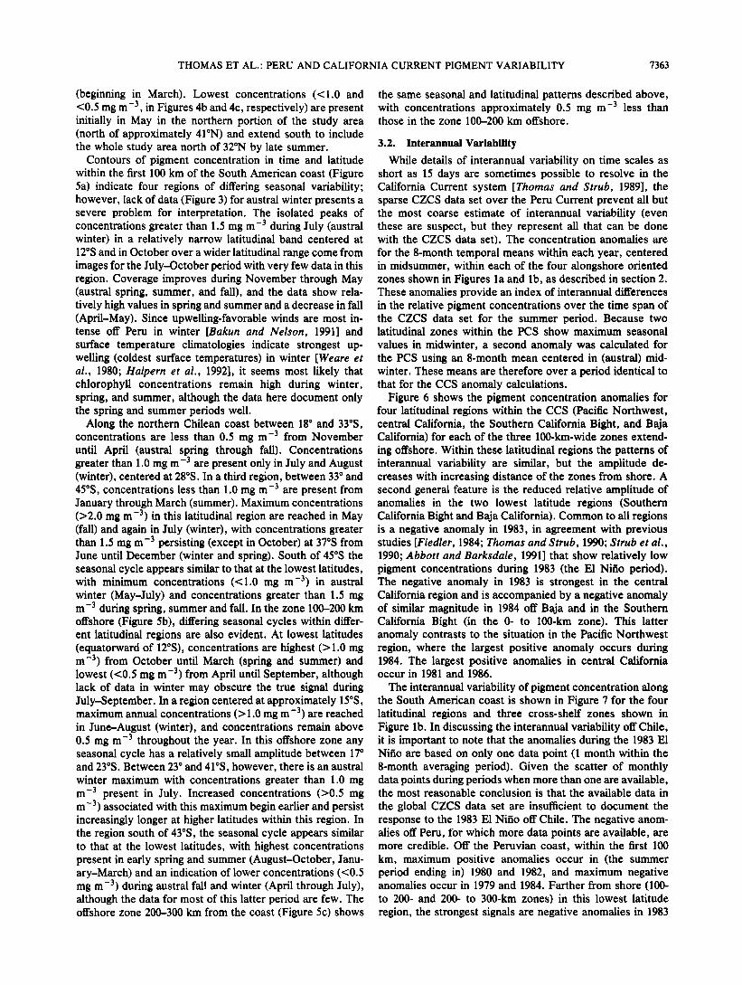
Contours of pigment concentration in time and latitude within the first 100 km of the South American coast (Figure 5a) indicate four regions of differing seasonal variability; however, lack of data (Figure 3) for austral winter presents a severe problem for interpretation. The isolated peaks of concentrations greater than 1.5 mg m -3 during July (austral winter) in a relatively narrow latitudinal band centered at 12øS and in October over a wider latitudinal range come from images for the July-October period with very few data in this region. Coverage improves during November through May (austral spring, summer, and fall), and the data show rela- tively high values in spring and summer and a decrease in fall (April-May). Since upwelling-favorable winds are most in- tense off Peru in winter [Bakun and Nelson, 1991] and surface temperature climatologies indicate strongest up- welling (coldest surface temperatures) in winter [Weare et al., 1980; Halpern et al., 1992], it seems most likely that chlorophyll concentrations remain high during winter, spring, and summer, although the data here document only the spring and summer periods well.
Along the northern Chilean coast between 18 ø and 33øS, concentrations are less than 0.5 mg m -3 from November until April (austral spring through fall). Concentrations greater than 1.0 mg m -3 are present only in July and August (winter), centered at 28øS. In a third region, between 33 ø and 45øS, concentrations less than 1.0 mg m -3 are present from January through March (summer). Maximum concentrations (>2.0 mg m -3) in this latitudinal region are reached in May (fall) and again in July (winter), with concentrations greater than 1.5 mg m -3 persisting (except in October) at 37øS from June until December (winter and spring). South of 45øS the seasonal cycle appears similar to that at the lowest latitudes, with minimum concentrations (<1.0 mg m -3) in austral winter (May-July) and concentrations greater than 1.5 mg m -3 during spring, summer and fall. In the zone 100-200 km offshore (Figure 5b), differing seasonal cycles within differ- ent latitudinal regions are also evident. At lowest latitudes (equatorward of 12øS), concentrations are highest (> 1.0 mg m -3) from October until March (spring and summer) and lowest (<0.5 mg m -3) from April until September, although lack of data in winter may obscure the true signal during July-September. In a region centered at approximately 15øS, maximum annual concentrations (> 1.0 mg m -3) are reached in June-August (winter), and concentrations remain above 0.5 mg m -3 throughout the year. In this offshore zone any seasonal cycle has a relatively small amplitude between 17 ø and 23øS. Between 23 ø and 41øS, however, there is an austral winter maximum with concentrations greater than 1.0 mg m -3 present in July. Increased concentrations (>0.5 mg m -3) associated with this maximum begin earlier and persist increasingly longer at higher latitudes within this region. In the region south of 43øS, the seasonal cycle appears similar to that at the lowest latitudes, with highest concentrations present in early spring and summer (August-October, Janu- ary-March) and an indication of lower concentrations (<0.5 mg m -3) during austral fall and winter (April through July), although the data for most of this latter period are few. The offshore zone 200-300 km from the coast (Figure 5c) shows
the same seasonal and latitudinal patterns described above, with concentrations approximately 0.5 mg m -3 less than those in the zone 100-200 km offshore.
3.2. Interannual Variability
While details of interannual variability on time scales as short as 15 days are sometimes possible to resolve in the California Current system [Thomas and Strub, 1989], the sparse CZCS data set over the Peru Current prevent all but the most coarse estimate of interannual variability (even these are suspect, but they represent all that can be done with the CZCS data set). The concentration anomalies are for the 8-month temporal means within each year, centered in midsummer, within each of the four alongshore oriented zones shown in Figures l a and lb, as described in section 2. These anomalies provide an index of interannual differences in the relative pigment concentrations over the time span of the CZCS data set for the summer period. Because two latitudinal zones within the PCS show maximum seasonal
values in midwinter, a second anomaly was calculated for the PCS using an 8-month mean centered in (austral) mid- winter. These means are therefore over a period identical to that for the CCS anomaly calculations.
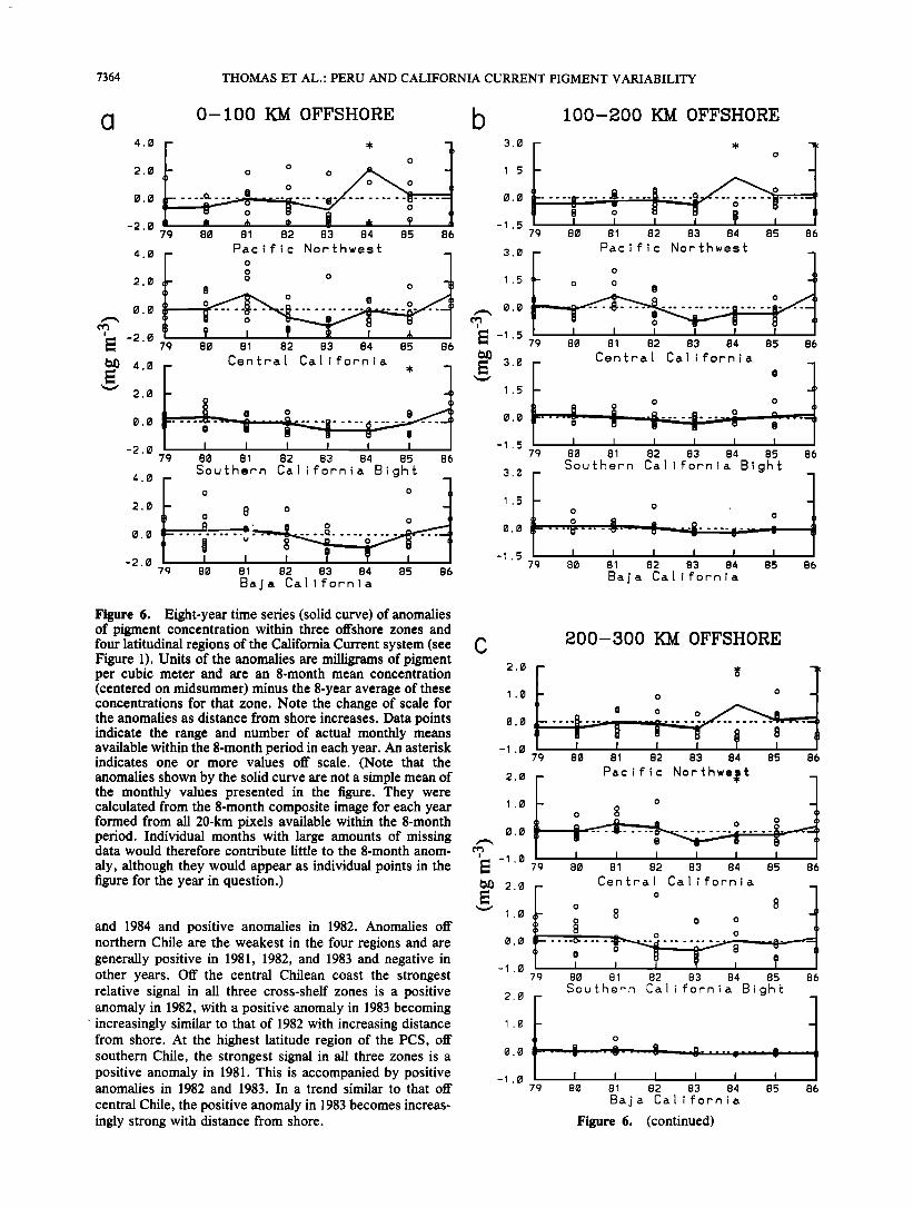
Figure 6 shows the pigment concentration anomalies for four latitudinal regions within the CCS (Pacific Northwest, central California, the Southern California Bight, and Baja California) for each of the three 100-kin-wide zones extend- ing offshore. Within these latitudinal regions the patterns of interannual variability are similar, but the amplitude de- creases with increasing distance of the zones from shore. A second general feature is the reduced relative amplitude of anomalies in the two lowest latitude regions (Southern California Bight and Baja California). Common to all regions is a negative anomaly in 1983, in agreement with previous studies [Fiedler, 1984; Thomas and Strub, 1990; Strub et al., 1990; Abbott and Barksdale, 1991] that show relatively low pigment concentrations during 1983 (the El Nifio period). The negative anomaly in 1983 is strongest in the central California region and is accompanied by a negative anomaly of similar magnitude in 1984 off Baja and in the Southern California Bight (in the 0- to 100-km zone). This latter anomaly contrasts to the situation in the Pacific Northwest region, where the largest positive anomaly occurs during 1984. The largest positive anomalies in central California occur in 1981 and 1986.
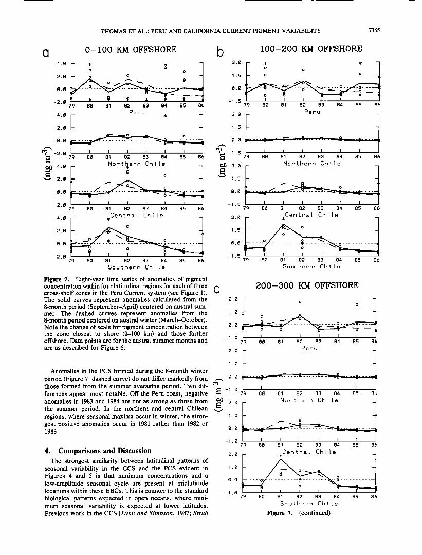
The interannual variability of pigment concentration along the South American coast is shown in Figure 7 for the four latitudinal regions and three cross-shelf zones shown in Figure lb. In discussing the interannual variability off Chile, it is important to note that the anomalies during the 1983 El Nifio are based on only one data point (1 month within the 8-month averaging period). Given the scatter of monthly data points during periods when more than one are available, the most reasonable conclusion is that the available data in
the global CZCS data set are insufficient to document the response to the 1983 El Nifio off Chile. The negative anom- alies off Peru, for which more data points are available, are more credible. Off the Peruvian coast, within the first 100 km, maximum positive anomalies occur in (the summer period ending in) 1980 and 1982, and maximum negative anomalies occur in 1979 and 1984. Farther from shore (100- to 200- and 200- to 300-km zones) in this lowest latitude region, the strongest signals are negative anomalies in 1983
7364 THOMAS ET AL.' PERU AND CALIFORNIA CURRENT PIGMENT VARIABILITY
0-100 OFFSHORE
4.0
t • o 2.0 o o o •o
79 80 81 82 83 84 85 86
4 0 Pac ;fic Northwest
õ o
-2 0 79 80 81 82 83 84 85 86 4 0 Cen•nai Cal ;fornia
20 o
...... • ..... • --9•L•$ ..... -20 I I I I I
79 80 81 82 83 84 85 86
Southern California Oigh• o
20 8 o
I I -20 79 80 81 82 83 84 85 86
Baja Cal ifornia
0 0
b 100-200 OFFSHORE
3 0
I I I I ?. I -15 79 80 81 82 83 84 85 86
30 Pacific Northwest
15 o 79 80 81 82 83 84 85 86
3 0 Central Cal iforn;a
15
o o o 00 o 0 ....
õ
-15 79 80 81 82 83 84 85 86
Southern California Bight
15 o o o o • a__._•_.• .......,_.
00• ..... • .... • ..... o .'' -15 I I I I I I 79 80 81 82 83 84 85 86
Ba3a California
0 0
Figure 6. Eight-year time series (solid curve) of anomalies of pigment concentration within three offshore zones and four latitudinal regions of the California Current system (see Figure 1). Units of the anomalies are milligrams of pigment per cubic meter and are an 8-month mean concentration (centered on midsummer) minus the 8-year average of these concentrations for that zone. Note the change of scale for the anomalies as distance from shore increases. Data points indicate the range and number of actual monthly means available within the 8-month period in each year. An asterisk indicates one or more values off scale. (Note that the anomalies shown by the solid curve are not a simple mean of the monthly values presented in the figure. They were calculated from the 8-month composite image for each year formed from all 20-km pixels available within the 8-month period. Individual months with large amounts of missing data would therefore contribute little to the 8-month anom-
aly, although they would appear as individual points in the figure for the year in question.)
and 1984 and positive anomalies in 1982. Anomalies off northern Chile are the weakest in the four regions and are generally positive in 1981, 1982, and 1983 and negative in other years. Off the central Chilean coast the strongest relative signal in all three cross-shelf zones is a positive anomaly in 1982, with a positive anomaly in 1983 becoming increasingly similar to that of 1982 with increasing distance from shore. At the highest latitude region of the PCS, off southern Chile, the strongest signal in all three zones is a positive anomaly in 1981. This is accompanied by positive anomalies in 1982 and 1983. In a trend similar to that off
central Chile, the positive anomaly in 1983 becomes increas- ingly strong with distance from shore.
c 200-300 KM OFFSHORE
o ' o -1.0
79 80 81 82 83 84 85 86
2.0 Pac; fic Northwest
10 o o o o
o o
• -1 0 79 80 81 82 83 84 85 86 • 2 0 Centra• Cal ;fornia
o •' 10 o 8 ß 0 o
8
0 0 ..... • .... o ...q....H.• -lO I I I
79 80 81 82 83 84 85 86
-1
Southern California Bight
o
0 ' -• •' a .•. ....... '•' ..... w - ,.. ' ' '' C ..... ., - - -
o I I I I I I 79 80 81 82 83 84 85 86
Ba j a Ca t i forn i a
Figure 6. (continued)
THOMAS ET AL.' PERU AND CALIFORNIA CURRENT PIGMENT VARIABILITY 7365
0-100 KM OFFSHORE
, -2 0
• 2 0
4.0 : oO o
2 o o.• 8 0 0
-2.0 86 79 80 81 82 83 84 85
4 0 Peru ß
0 0 .... •- ........
I I I I I I 79 80 81 82 83 84 85
-2 0
4 0
2 0
0 0
-2 0
86
Nor"•:h,),ern Ch i [ e 8 o
79 80 81 82 83 84 85 86
Centrat Chile ,
o
7g 80 81 82 83 84 85 86
Sou f. hern Ch i[e
b 100-200 KM OFFSHORE
3 0
1 5 o o
79 80 81 82 83 84 85 86
3 0 Peru _
0 0 , _._,., _. • - • ..•. o 1 ___ ----., - • - ... .... • .---,',_.•...
I I I I I I T 79 80 81 82 83 84 85 86
Northern Chi[e
1 5
..... .... 79 80 81 82 83 84 85 86
3 0 Central Oh i le ,
1 5
o o
79 80 81 82 83 84 85 86
-1 5
-1 5
-1 5
Southern Chi l e
Figure 7. Eight-year time series of anomalies of pigment concentration within four latitudinal regions for each of three cross-shelf zones in the Peru Current system (see Figure 1). C The solid curves represent anomalies calculated from the 8-month period (September-April) centered on austral sum- mer. The dashed curves represent anomalies from the 8-month period centered on austral winter (March-October). Note the change of scale for pigment concentration between the zone closest to shore (0-100 km) and those farther offshore. Data points are for the austral summer months and
200-300 KM OFFSHORE
2 0
1 0
0 0
-1 0
o o
79 80 81 82 83 84 85 86
are as described for Figure 6. P e r u 2 0
1 0
Anomalies in the PCS formed during the 8-month winter period (Figure 7, dashed curve) do not differ markedly from • ½ ½ - --' --- -- ----•-• ..... e- ---• those formed from the summer averaging period. Two dif- ? ferences appear most notable. Off the Peru coast, negative • -• 0 I I I I 79 80 81 82 83 84 85 86
anomalies in 1983 and 1984 are not as strong as those from • 2 0 Nor •hern Oh i [ e the summer period In the northern and central Chilean ß
regions, where seasonal maxima occur in winter, the stron- • o
gest positive anomalies occur in 1981 rather than 1982 or • .... ..•• 1983. o o - -•:g -,•-- .......... o I • I I I
4. Comparisons and Discussion The strongest similarity between latitudinal patterns of
seasonal variability in the CCS and the PCS evident in Figures 4 and 5 is that minimum concentrations and a low-amplitude seasonal cycle are present at midlatitude locations within these EBCs. This is counter to the standard
biological patterns expected in open oceans, where mini- mum seasonal variability is expected at lower latitudes. Previous work in the CCS [Lynn and Simpson, 1987; Strub
-1 79 80 81 82 83 84 85 86
2 0 Central Ch i le
1 0 * o 0 0
79 80 81 82 83 84 85 86
Sou•:hern Chi l e
Figure 7. (continued)
7366 THOMAS ET AL.' PERU AND CALIFORNIA CURRENT PIGMENT VARIABILITY
-10
-15
-2o
-25
-3o
-55
-40
-45
-50
-10
-15
-2O
-25
-3O
-35
-45
-5O
Summer Fall Winter Spring -85 -80 -75 -70
• 2
. -t t/; ,,1. "7' -,
. ,, %. -. *. %. 1-,o
-85 -80 -75 -70
-85 -80 -75 -70
-85 -80 -75 -70
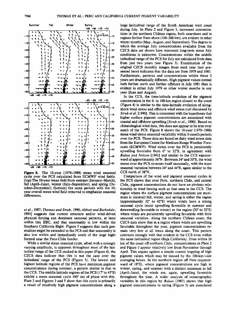
Filure 8. The 10-year (1979-1988) mean wind seasonal cycle over the PCS calculated from ECMWF wind fields. (top) The 10-year mean field from summer (January-March), fall (April-June), winter (July-September), and spring (Oc- tober-December); (bottom) the same periods with the 10- year overall mean wind field removed to emphasize seasonal differences.
et al., 1987; Thomas and $trub, 1990; Abbott and Barksdale, 1991] suggests that current structure and/or wind-driven physical forcing can dominate seasonal patterns, at least within this EBC, and that seasonality is low within the Southern California Bight. Figure 5 suggests that such gen- eralities might be extended to the PCS and that seasonality is also low within and immediately south of the large bight formed near the Peru-Chile border.
While a similar mean seasonal cycle, albeit with a strongly varying amplitude, is apparent throughout most of the lati- tudinal range of the CCS studied in this paper (Figure 4), the CZCS data indicate that this is not the case over the
latitudinal range of the PCS (Figure 5). The lowest and highest latitude regions of the PCS have maximum pigment concentrations during summer, a pattern similar to that in the CCS. The middle latitude regions of the PCS (17 ø to 45øS) exhibit a mean seasonal cycle 180 ø out of phase with this. Plate 2 and Figures 3 and 5 show that this cycle is primarily a result of relatively high pigment concentrations along a
large latitudinal range of the South American west coast during July. In Plate 2 and Figure 3, increased concentra- tions in the northern Chilean region, both nearshare and in regions farther from shore (100-300 km), are evident in other winter months (May, August, and September). The degree to which the average July concentrations available from the CZCS data set shown here represent long-term mean July conditions is unknown. Concentrations within the middle
latitudinal range of the PCS for July are calculated from data from just two years (see Figure 3). Examination of the original CZCS monthly images from each year (not pre- sented here) indicates that the data are from 1979 and 1981. Furthermore, patterns and concentrations within these 2 years are dramatically different. High pigment values extend both farther north and farther offshore in July 1981 than is evident in either July 1979 or other winter months in any year (June and August).
In the CCS, the time-latitude evolution of the pigment concentration in the 0- to 100-km region closest to the coast (Figure 4) is similar to the time-latitude evolution of along- shore wind stress and offshore wind stress curl discussed by Strub et al. [1990]. This is consistent with the hypothesis that higher surface pigment concentrations are associated with coastal and offshore upwelling [Strub et al., 1990]. Based on climatological wind data, this does not appear to be true over much of the PCS. Figure 8 shows the 10-year (1979-1988) mean wind stress seasonal variability within 3-month periods over the PCS. These data are based on daily wind stress data from the European Centre for Medium-Range Weather Fore- casts (ECMWF). Wind stress over the PCS is persistently upwelling favorable from 6 ø to 32øS, in agreement with Bakun and Nelson [1991] and similar to the CCS equator- ward of approximately 36øN. Between 34 ø and 50øS, the wind stress over the PCS reverses itself seasonally, with the most seasonal variation between 34 ø and 44øS, again similar to the CCS north of 38øN.
Comparison of the wind and pigment seasonal cycles in the PCS shows that over Peru, northern Chile, and central Chile, pigment concentrations do not have an obvious rela- tionship to wind forcing such as that seen in the CCS. The region where the surface pigment concentrations are maxi- mum in (austral) fall, winter, and spring is either the region (approximately 32 ø to 42øS) where winds have a strong seasonal cycle (most upwelling favorable in summer and downwelling favorable in winter) or the region (20 ø to 32øS) where winds are persistently upwelling favorable with little seasonal variation. Along the northern Chilean coast, the CZCS data show that in a region where winds are upwelling favorable throughout the year, pigment concentrations re- main very low at all times along the coast. This pattern contrasts strongly with that evident in the CCS even within the same latitudinal region (Baja California). Even within 20 km of the coast off northern Chile, concentrations in Plate 2 and Figure 3 appear relatively low from November through April. This argues against a simple coastal trapping of high pigment values which may be missed by the 100-km-wide averaging boxes. In the northern region off Peru (equator- ward of 18øS), where pigment concentrations are high in winter, spring, and summer with a distinct minimum in fall (April-June), the winds are, again, upwelling favorable throughout the year. A wider analysis of oceanographic variables in this region by Bakun [1987] shows that high pigment concentrations in spring (Figure 5) are associated
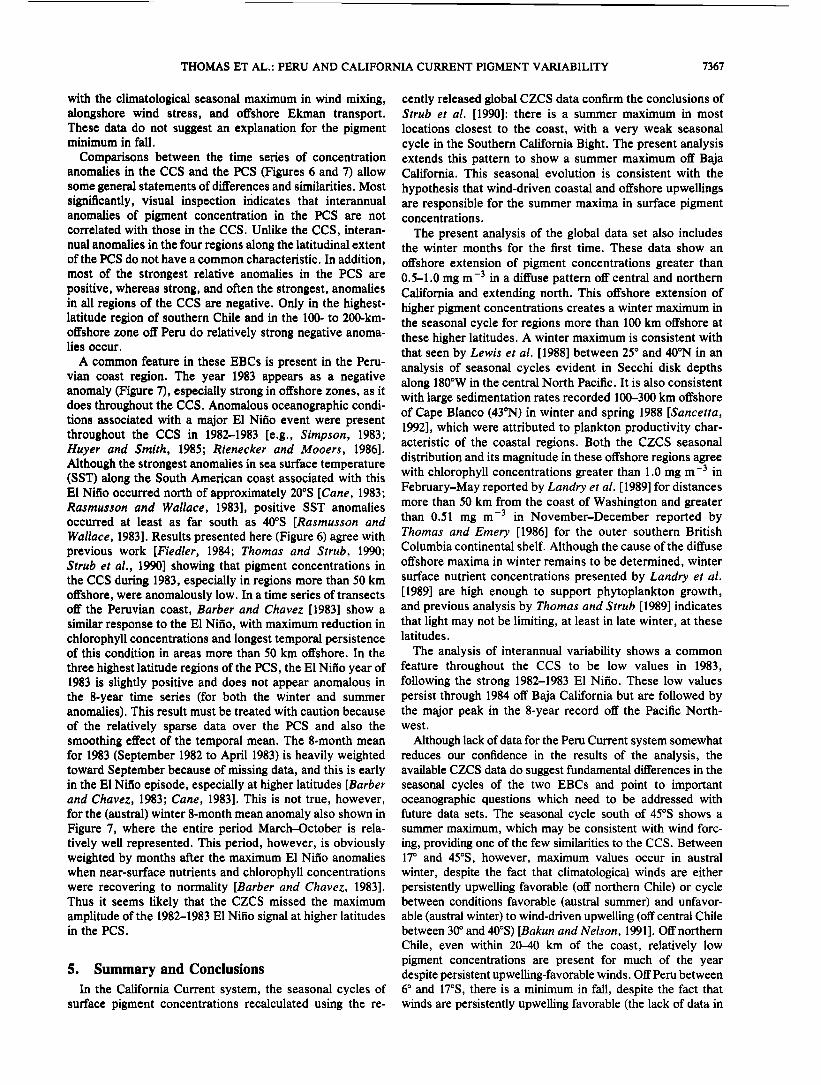
THOMAS ET AL.' PERU AND CALIFORNIA CURRENT PIGMENT VARIABILITY 7367
with the climatological seasonal maximum in wind mixing, alongshore wind stress, and offshore Ekman transport. These data do not suggest an explanation for the pigment minimum in fall.
Comparisons between the time series of concentration anomalies in the CCS and the PCS (Figures 6 and 7) allow some general statements of differences and similarities. Most significantly, visual inspection indicates that interannual anomalies of pigment concentration in the PCS are not correlated with those in the CCS. Unlike the CCS, interan- nual anomalies in the four regions along the latitudinal extent of the PCS do not have a common characteristic. in addition, most of the strongest relative anomalies in the PCS are positive, whereas strong, and often the strongest, anomalies in all regions of the CCS are negative. Only in the highest- latitude region of southern Chile and in the 100- to 200-km- offshore zone off Peru do relatively strong negative anoma- lies occur.
A common feature in these EBCs is present in the Peru- vian coast region. The year 1983 appears as a negative anomaly (Figure 7), especially strong in offshore zones, as it does throughout the CCS. Anomalous oceanographic condi- tions associated with a major E1 Nifio event were present throughout the CCS in 1982-1983 [e.g., Simpson, 1983; Huyer and Smith, 1985; Rienecker and Mooers, 1986]. Although the strongest anomalies in sea surface temperature (SST) along the South American coast associated with this E1 Nifio occurred north of approximately 20øS [Cane, 1983; Rasmusson and Wallace, 1983], positive SST anomalies occurred at least as far south as 40øS [Rasmusson and Wallace, 1983]. Results presented here (Figure 6) agree with previous work [Fiedler, 1984; Thomas and Strub, 1990; Strub et al., 1990] showing that pigment concentrations in the CCS during 1983, especially in regions more than 50 km offshore, were anomalously low. In a time series of transects off the Peruvian coast, Barber and Chavez [1983] show a similar response to the E1 Nifio, with maximum reduction in chlorophyll concentrations and longest temporal persistence of this condition in areas more than 50 km offshore. In the
three highest latitude regions of the PCS, the E1Nifio year of 1983 is slightly positive and does not appear anomalous in the 8-year time series (for both the winter and summer anomalies). This result must be treated with caution because of the relatively sparse data over the PCS and also the smoothing effect of the temporal mean. The 8-month mean for 1983 (September 1982 to April 1983) is heavily weighted toward September because of missing data, and this is early in the E1 Nifio episode, especially at higher latitudes [Barber and Chavez, 1983; Cane, 1983]. This is not true, however, for the (austral) winter 8-month mean anomaly also shown in Figure 7, where the entire period March-October is rela- tively well represented. This period, however, is obviously weighted by months after the maximum E1 Nifio anomalies when near-surface nutrients and chlorophyll concentrations were recovering to normality [Barber and Chavez, 1983]. Thus it seems likely that the CZCS missed the maximum amplitude of the 1982-1983 E1Nifio signal at higher latitudes in the PCS.
$. Summary and Conclusions In the California Current system, the seasonal cycles of
surface pigment concentrations recalculated using the re-
cently released global CZCS data confirm the conclusions of Strub et al. [1990]' there is a summer maximum in most locations closest to the coast, with a very weak seasonal cycle in the Southern California Bight. The present analysis extends this pattern to show a summer maximum off Baja California. This seasonal evolution is consistent with the
hypothesis that wind-driven coastal and offshore upwellings are responsible for the summer maxima in surface pigment concentrations.
The present analysis of the global data set also includes the winter months for the first time. These data show an
offshore extension of pigment concentrations greater than 0.5-1.0 mg m -3 in a diffuse pattern off central and northern California and extending north. This offshore extension of higher pigment concentrations creates a winter maximum in the seasonal cycle for regions more than 100 km offshore at these higher latitudes. A winter maximum is consistent with that seen by Lewis et al. [1988] between 25 ø and 40øN in an analysis of seasonal cycles evident in Secchi disk depths along 180øW in the central North Pacific. It is also consistent with large sedimentation rates recorded 100-300 km offshore of Cape Blanco (43øN) in winter and spring 1988 [Sancetta, 1992], which were attributed to plankton productivity char- acteristic of the coastal regions. Both the CZCS seasonal distribution and its magnitude in these offshore regions agree with chlorophyll concentrations greater than 1.0 mg m -3 in February-May reported by Landry et al. [1989] for distances more than 50 km from the coast of Washington and greater than 0.51 mg m -3 in November-December reported by Thomas and Emery [1986] for the outer southern British Columbia continental shelf. Although the cause of the diffuse offshore maxima in winter remains to be determined, winter surface nutrient concentrations presented by Landry et al. [1989] are high enough to support phytoplankton growth, and previous analysis by Thomas and Strub [1989] indicates that light may not be limiting, at least in late winter, at these latitudes.
The analysis of interannual variability shows a common feature throughout the CCS to be low values in 1983, following the strong 1982-1983 E1 Nifio. These low values persist through 1984 off Baja California but are followed by the major peak in the 8-year record off the Pacific North- west.
Although lack of data for the Peru Current system somewhat reduces our confidence in the results of the analysis, the available CZCS data do suggest fundamental differences in the seasonal cycles of the two EBCs and point to important oceanographic questions which need to be addressed with future data sets. The seasonal cycle south of 45øS shows a summer maximum, which may be consistent with wind forc- ing, providing one of the few similarities to the CCS. Between 17 ø and 45øS, however, maximum values occur in austral winter, despite the fact that climatological winds are either persistently upwelling favorable (off northern Chile) or cycle between conditions favorable (austral summer) and unfavor- able (austral winter) to wind-driven upwelling (off central Chile between 30 ø and 40øS) [Bakun and Nelson, 1991]. Off northern Chile, even within 20-40 km of the coast, relatively low pigment concentrations are present for much of the year despite persistent upwelling-favorable winds. Off Peru between 6 ø and 17øS, there is a minimum in fall, despite the fact that winds are persistently upwelling favorable (the lack of data in
7368 THOMAS ET AL.' PERU AND CALIFORNIA CURRENT PIGMENT VARIABILITY
winter may mask what is really a broad winter, spring, and summer maximum).
The analysis of interannual variability off South America shows a decrease in relative pigment concentration in off- shore zones off the Peru coast (lowest latitudes) after the 1982-1983 E1 Nifio. This parallels observations within the CCS during 1983 which show that maximum differences due to E1 Nifio conditions were offshore and that very nearshore pigment concentrations remained high [Fiedler, 1984; Tho- mas and Strub, 1990]. This pattern is also in agreement with in situ observations from a cross-shelf transect at 5øS pre- sented by Barber and Chavez [1983]. Off Chile, the historical CZCS data are too sparse to document interannual variabil- ity with any confidence.
The most robust result of our analysis concerns the seasonal cycle off Chile between 30 ø and 40øS, where the spring-summer data coverage is best and where the seasonal increase in upwelling-favorable winds is greatest during the same period (October-March). Here, pigment concentra- tions in the 100 km next to the coast only briefly exceed 1.5 mg m -3 dropping below 1.0 mg m -3 in summer. This contrasts to values greater than 3.0-4.0 mg m -3 during spring and summer within 100 km of the coast in the region of seasonality in upwelling-favorable winds off California. Thus forces other than large-scale seasonal wind forcing appear to dominate the seasonal cycles of surface pigment concentration over large portions of the PCS.
The significance of this difference goes beyond the phyto- plankton response to local wind forcing. It raises the question of whether the surface signature of the phytoplankton standing stock (as seen from a satellite) can be used as an indicator of the overall productivity of the coastal ocean system at the higher trophic levels. The productivity of the coastal ocean off Chile, as measured by the harvest of phytoplankton-eating fish species (anchovies and sardines), is reportedly 5 to 20 times greater than that off California (P. Smith and R. Parrish, personal communications, 1992). The harvest of predator fish species such as jack mackerel is also large. Why, then, do the satellite color data suggest much lower surface concentrations of chlorophyll (and phytoplankton)? Are the phytoplankton located deeper in the water column than the satellite can see? Is it possible that higher concentrations of phytoplankton exist in a very narrow nearshore region difficult to resolve in this relatively low spatial resolution data set? Do very high primary productivity rates maintain the fishery, with biomass being so heavily grazed that higher concentrations either do not build up or do not spread offshore? These are questions that the CZCS data set can only pose. Answers rely on the combination of future field data and more reliable satellite color data.
Thus, acknowledging the relative lack of data, the time series of CZCS data suggest that there are fundamental differences in the seasonal variabilities of surface pigment concentrations in the Peru and California Current systems, even though large-scale wind forcing is similar. A more complete understanding of this variability and its relation to wind forcing, upwelling, and horizontal transport within these current systems will be possible only when a more complete data set becomes available. As always, the need for in situ observations over a wide range of spatial and temporal scales is tantamount. In the future, combinations of pigment data from SeaWiFS (and other) sensors, current data from TOPEX and other altimeters, and wind data from
scatterometers should clarify the relationships glimpsed only partially and imperfectly with the CZCS data set.
Appendix The diffuse pattern of surface pigment concentration val-
ues, shown stretching far offshore in Plate 1 and Figure 4, is similar to the pattern caused by the single Rayleigh scatter- ing atmospheric correction used in previous versions of the CZCS data, although much lower in magnitude [Strub et al., 1990] (hereinafter referred to as SJTA). Although the global CZCS data set uses the multiple Rayleigh scattering algo- rithm [Gordon et al., 1988; Feldman et al., 1989], it is natural to wonder how much systematic error may still be caused by incompletely corrected atmospheric scattering at high sun- satellite angles (high latitude, winter).
SJTA developed a technique for estimating this error empirically for the previous data. That technique is repeated here. The assumptions of the technique are that (1) the error increases monotonically with latitude; (2) the error should have the greatest magnitude at times around the winter solstice; and (3) winter values of pigment concentration far offshore are uniformly low, without a monotonic increase with higher latitude.
The technique simply uses the CZCS pigment concentra- tion values in a north-south band far from the coast in an
empirical orthogonal function (EOF) analysis and examines the space and time series for the properties listed as assump- tions 1 and 2 above. Since SJTA used data from the West
Coast time series, which extended only 5 ø from the coast, they formed a 2.5ø-wide band separated from the coast by 2.5 ø of longitude. The first EOF accounted for 71% of the variance, with a temporal function that had maximum values of 3.0 in December and January and approximately 0.0 in June and July. The spatial function ramped up from approx- imately 0 at 25øN to 1.3 between 40 ø and 50øN. Thus errors of approximately 4.0 mg m -3 occurred in winter north of 40øN.
Although the global data set is not restricted to the region near the coast, there are more data for that region. For this reason and in order to facilitate a comparison to the results of SJTA, the technique was applied to the global data set in two latitudinal bands: one based on 1 ø latitude by 2.5 ø longitude blocks separated from the coast by 2.5 ø of longi- tude, and another based on 1 ø latitude by 3.0 ø longitude blocks separated from the coast by 5.0 ø of longitude. The data are from the first 4 years of the global data set (1979-1982), when data coverage was better. The results are shown in Figures Ala and Alb, respectively.
The average seasonal time series of each function show low values (0.1-0.2) in spring and summer and higher values (0.5-0.9) in fall and winter. The spatial functions show localized maxima superimposed on a gradual increase with latitude which is more evident farther from shore. An
identical dashed curve based on the increase in minimum
values from the more offshore band (Figure A lb) has been drawn by hand in both figures. The fact that it fits the minimum values in Figure A 1 a gives us some confidence that it describes an upper estimate of the bias caused by uncor- rected atmospheric scattering (or other systematic optical effects). Using the more offshore band, where we expect lower true pigment values, the maximum value for the averaged seasonal time series is 0.4 and occurs in November
THOMAS ET AL.' PERU AND CALIFORNIA CURRENT PIGMENT VARIABILITY 7369
1.0
0.8
0.6
0.4
0.2
;5.5 ! 3.0
'2.5
2.0
1.5 1.0 0.5
Jon Feb Mot Apr MoyJun Jul Aug Sep Oct Nov Dec Time sir;el
A A ....... , I • 0.0 .-.." .......
20 50 40 50
Latitude
l.2 1.0
•, o.s
8
0.2
......... I ......... I ....
20 •0 40 50
,•' 2.5 ,..,,• 2.0
l.5 0.5
0.0
Jon Feb Mot Apr MoyJun Jul AUg Sep Oct Nov Dec Time sir;el Lot;tude ("N)
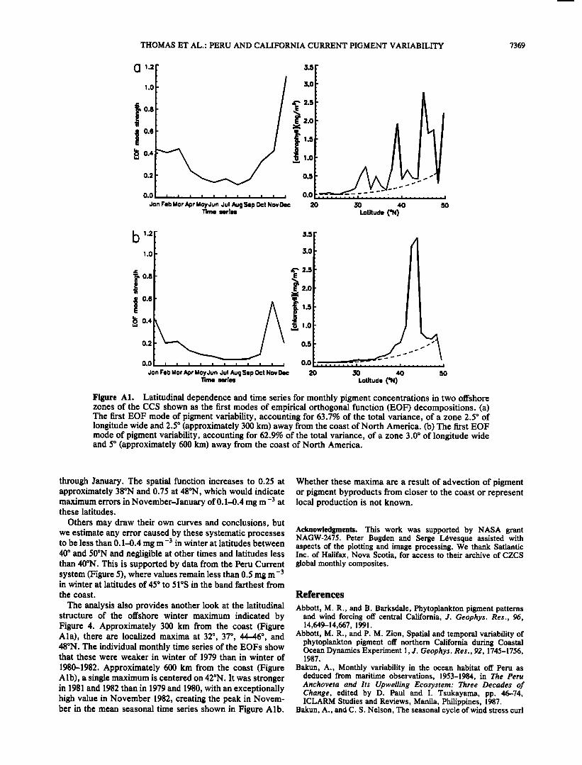
Figure AI. Latitudinal dependence and time series for monthly pigment concentrations in two offshore zones of the CCS shown as the first modes of empirical orthogonal function (EOF) decompositions. (a) The first EOF mode of pigment variability, accounting for 63.7% of the total variance, of a zone 2.5 ø of longitude wide and 2.5 ø (approximately 300 km) away from the coast of North America. (b) The first EOF mode of pigment variability, accounting for 62.9% of the total variance, of a zone 3.0 ø of longitude wide and 5 ø (approximately 600 km) away from the coast of North America.
through January. The spatial function increases to 0.25 at approximately 38øN and 0.75 at 48øN, which would indicate maximum errors in November-January of 0.1-0.4 mg m -3 at these latitudes.
Others may draw their own curves and conclusions, but we estimate any error caused by these systematic processes to be less than 0.1-0.4 mg m -3 in winter at latitudes between 40 ø and 50øN and negligible at other times and latitudes less than 40øN. This is supported by data from the Peru Current system (Figure 5), where values remain less than 0.5 mg m -3 in winter at latitudes of 45 ø to 51 øS in the band farthest from the coast.
The analysis also provides another look at the latitudinal structure of the offshore winter maximum indicated by Figure 4. Approximately 300 km from the coast (Figure Ala), there are localized maxima at 32 ø, 37 ø, 4 a. •.6 ø, and 48øN. The individual monthly time series of the EOFs show that these were weaker in winter of 1979 than in winter of
1980-1982. Approximately 600 km from the coast (Figure Alb), a single maximum is centered on 42øN. It was stronger in 1981 and 1982 than in 1979 and 1980, with an exceptionally high value in November 1982, creating the peak in Novem- ber in the mean seasonal time series shown in Figure A lb.
Whether these maxima are a result of advection of pigment or pigment byproducts from closer to the coast or represent local production is not known.
Acknowledgments. This work was supported by NASA grant NAGW-2475. Peter Bugden and Serge L6vesque assisted with aspects of the plotting and image processing. We thank Satlantic Inc. of Halifax, Nova Scotia, for access to their archive of CZCS global monthly composites.
References
Abbott, M. R., and B. Barksdale, Phytoplankton pigment patterns and wind forcing off central California, J. Geophys. Res., 96, 14,649-14,667, 1991.
Abbott, M. R., and P.M. Zion, Spatial and temporal variability of phytoplankton pigment off northern California during Coastal Ocean Dynamics Experiment 1, J. Geophys. Res., 92, 1745-1756, 1987.
Bakun, A., Monthly variability in the ocean habitat off Peru as deduced from maritime observations, 1953-1984, in The Peru Anchoveta and Its Upwelling Ecosystem: Three Decades of Change, edited by D. Paul and I. Tsukayama, pp. 46-74, ICLARM Studies and Reviews, Manila, Philippines, 1987.
Bakun, A., and C. S. Nelson, The seasonal cycle of wind stress curl
7370 THOMAS ET AL.: PERU AND CALIFORNIA CURRENT PIGMENT VARIABILITY
in sub-tropical eastern boundary current regions, J. Phys. Ocean- ogr., 21, 1815-1834, 1991.
Barber, R. T., and F. P. Chavez, Biological consequences of El Nifio, Science, 222, 1203-1210, 1983.
Barber, R. T., and F. P. Chavez, Ocean variability in relation to living resources during the 1982-83 El Nifio, Nature, 319, 279- 285, 1986.
Cane, M. A., Oceanographic events during El Nifio, Science, 222, 1189-1194, 1983.
Espinoza, F. R., A. Maoxiang, and S. Neshyba, Surface water motion off Chile revealed in satellite images of surface chlorophyll and temperatures, in Proceedings, International Conference on Marine Resources of the Pacific, edited by P.M. Arana, pp. 41-57, Universidad Catolica de Valparaiso, Valparaiso, Chile, 1983.
Feldman, G., N. Kuring, C. Ng, W. Esaias, C. McClain, J. Elrod, N. Maynard, D. Endres, R. Evans, J. Brown, S. Walsh, M. Carle, and G. Podesta, Ocean color: Availability of the global data set, Eos Trans. AGU, 70, 634-641, 1989.
Fiedler, P. C., Satellite observations of the 1982-1983 El Nifio along the U.S. Pacific coast, Science, 224, 1251-1254, 1984.
Gordon, H. R., and D. J. Castano, The coastal zone color scanner atmospheric correction algorithm: Multiple scattering effects, Appl. Opt., 26, 2111-2122, 1987.
Gordon, H. R., D. K. Clark, J. W. Brown, O. B. Brown, R. H. Evans, and W. W. Broenkow, Phytoplankton pigment concentra- tions in the Middle Atlantic Bight: Comparisons of ship determi- nations and CZCS estimates, Appl. Opt., 22, 20-36, 1983a.
Gordon, H. R., J. W. Brown, O. B. Brown, R. H. Evans, and D. K. Clark, Nimbus 7 CZCS: Reduction of its radiometric sensitivity with time, Appl. Opt., 22, 3929-3931, 1983b.
Gordon, H. R., J. W. Brown, and R. H. Evans, Exact Rayleigh scattering calculations for use with the Nimbus-7 coastal zone color scanner, Appl. Opt., 27, 862-871, 1988.
Halpern, D., W. Knauss, O. Brown, and F. Wentz, An atlas of monthly mean distributions of SSMI surface wind speed, Argos buoy drift, AVHRR/2 sea surface temperature, and ECMWF surface wind components during 1989, JPL Publ. 92-17, 112 pp., Jet Propul. Lab., Pasadena, Calif., 1992.
Huyer, A. E., and R. L. Smith, The signature of El Nifio off Oregon, 1982-1983, J. Geophys. Res., 90, 7133-7142, 1985.
Landry, M. R., J. R. Postel, W. K. Peterson, and J. Newman, Broad-scale distributional patterns of hydrographic variables on the Washington/Oregon sheif, in Coastal Oceanography of Wash- ington and Oregon, edited by M. R. Landry and B. M. Hickey, pp. 1-40, Elsevier, New York, 1989.
Lewis, M. R., N. Kuring, and C. Yentsch, Global patterns of ocean transparency: Implications for the new production of the open ocean, J. Geophys. Res., 93, 6847-6856, 1988.
Lynn, R. J., and J. J. Simpson, The California Current system: The seasonal variability of its physical characteristics, J. Geophys. Res., 92, 12,947-12,966, 1987.
Michaelsen, J., X. Zhang, and R. C. Smith, Variability of pigment biomass in the California Current system as determined by satellite imagery, 2, Temporal variability, J. Geophys. Res., 93, 10,883-10,896, 1988.
Minas, H. J., M. Minas, and T. T. Packard, Productivity in upwelling areas deduced from hydrographic and chemical fields, Limnol. Oceanogr., 31, 1182-1206, 1986.
Mueller, J. L., Nimbus 7 CZCS: Confirmations of its radiometric sensitivity decay rate through 1982, Appl. Opt., 24, 1043-1047, 1985.
Pelaez, J., and J. A. McGowan, Phytoplankton pigment patterns in
the California Current as determined by satellite, Limnol. Ocean- ogr., 31,927-950, 1986.
Rasmusson, E. M., and J. M. Wallace, Meteorological aspects of the El Nifio/Southern Oscillation, Science, 222, 1195-1202, 1983.
Rienecker, M. M., and C. N. K. Mooers, The 1982-1983 El Nifio signal off northern California, J. Geophys. Res., 91, 6597-6608, 1986.
Sancetta, C., Comparison of phytoplankton in sediment trap time series and surface sediments along a productivity gradient, Pa- leoceanography, 7, 183-194, 1992.
Schulz, S., A comparison of primary production in upwelling regions off northwest and southwest Africa, Rapp. P. V. Reun. Cons. Petra. Int. Explor. Met, 180, 202-204, 1982.
Simpson, J. J., Large-scale thermal anomalies in the California Current during the 1982-1983 El Nifio, Geophys. Res. Lett., 10, 937-940, 1983.
Smith, R. C., X. Zhang, and J. Michaelsen, Variability of pigment biomass in the California Current system as determined by satellite imagery, 1, Spatial variability, J. Geophys. Res., 93, 10,863-10,882, 1988.
Smith, R. L., A comparison of the structure and variability of the flow field in three coastal upwelling regions: Oregon, northwest Africa and Peru, in Coastal Upwelling, Coastal Estuarine Sci., vol. 1, edited by F. A. Richards, pp. 107-118, AGU, Washington, D.C., 1981.
Strub, P. T., J. S. Allen, A. Huyer, R. L. Smith, and R. C. Beardsley, Seasonal cycles of currents, temperatures, winds, and sea level over the northeast Pacific continental sheif: 35'N to
48'N, J. Geophys. Res., 92, 1507-1526, 1987. Strub, P. T., C. James, A. C. Thomas, and M. R. Abbott, Seasonal
and nonseasonal plankton concentrations, hydrography, and sat- ellite-measured sea surface temperature, J. Geophys. Res., 95, 11,501-11,530, 1990.
Thomas, A. C., and W. J. Emery, Winter hydrography and plankton distribution on the southern British Columbia continental sheif, Can. J. Fish. Aquat. Sci., 43, 1249-1258, 1986.
Thomas, A. (2., and P. T. Strub, Interannual variability in phyto- plankton pigment distribution during the spring transition along the west coast of North America, J. Geophys. Res., 94, 18,095- 18,117, 1989.
Thomas, A. C., and P. T. Strub, Seasonal and interannual variability of pigment concentrations across a California Current frontal zone, J. Geophys. Res., 95, 13,023-13,042, 1990.
Uribe, T., and S. Neshyba, Phytoplankton pigments from the Nimbus-7 coastal zone color scanner: Coastal waters of Chile
from 18' to 40'S, in Proceedings, International Conference ott Marine Resources of the Pacific, edited by P.M. Arana, pp. 33-40, Universidad Catolica de Valparaiso, Valparaiso, Chile, 1983.
Weare, B.C., P. T. Strub, and M.D. Samuel, Marine climate atlas of the tropical Pacific Ocean, Contrib. in Atmos. Sci., 20, 147 pp., Univ. of Calif., Davis, 1980.
F. Huang and A. C. Thomas, Atlantic Center for Remote Sensing of the Oceans, 6155 North Street, Suite 301, Halifax, Nova Scotia, Canada B3K 3R3.
C. James and P. T. Strub, College of Oceanic and Atmospheric Sciences, Oregon State University, Corvallis, OR 97331.
(Received September 14, 1992; revised April 28, 1993; accepted August 4, 1993.)