comparison of turbulence models in openfoam for 3d

AiMTAdvances in Military Technology

Vol. 11, No. 2 (2016), pp. 239-251ISSN 1802-2308, eISSN 2533-4123

DOI 10.3849/aimt.01131

Comparison of Turbulence Models in OpenFOAM for 3D Simulation of Gas Flow

in Solid Propellant Rocket Engine

P. Konečný1* and R. Ševčík2

1 University of Defence, Brno, Czech Republic 2 Masaryk University, Brno, Czech Republic

The manuscript was received on 26 May 2016 and was accepted after revision for publication on 25 December 2016.

Abstract:

The aim of this paper is to compare various mathematical models simulating the turbu-lent flow in a solid propellant rocket engine. For comparison, the most frequently used models were chosen for simulations of flow in the S5 rocket engine. For this type of engine experimental data are available allowing comparison of the simulations with reality. The LES Smagorinsky model provided the best results, while type RANS models appeared to be less suitable for this task.

Keywords:

turbulent flow, turbulent model, solid propellant rocket engine, OpenFOAM

1. Introduction During the development of a new numerical model for a solid propellant rocket engine we previously described turbulent flow [1]. This paper, on the other hand, aims to compare selected models of turbulent flow of the OpenFOAM framework.

For numerical simulation of the Navier-Stokes equations, the method of Direct Numerical Simulation (DNS) is considered as the most accurate. It allows the accurate simulating of the full spectrum of vortical structures at the appropriate temporal and spatial resolution. However, this method is very computationally demanding, the smallest cells of computational mesh must correspond to the order of the size of the smallest eddies and their number extremely increases with the value of the Reynolds number. For research purposes, this method is the most accurate one. Nevertheless, for many engineering applications a proper turbulence model is sufficient. As for turbu-

* Corresponding author: Department of Weapons and Ammunition, University of Defence,

Kounicova 65, Brno, Czech Republic. Phone: +420 973 44 20 37, fax: +420 973 44 37 72, E-mail: [email protected]

240 P. Konecný and R. Ševcík

lence models, there are many options to choose the most suitable one, and it is neces-sary to understand their characteristics, advantages and limitations.

2. Available Turbulence Models To find out which model of turbulence in OpenFOAM 2.3 can be used, we performed the “banana test” as described in [2]. For Large Eddy Simulation (LES) models we get a listing:

DeardorffDiffStress LRRDiffStress Smagorinsky SpalartAllmaras SpalarAllmarasDDES SpalartAllmarasIDDES dynLagrangian dynOneEqEddy homogenousDynOneEqEddy homogenousDynSmagorinsky kOmegaSSTSAS laminar mixedSmagorinsky oneEqEddy spectEddyVisc

For Reynolds-Averaged Simulation (RANS) models we get a listing: LRR LamBremhorstKE LaunderGibsonRSTM LaunderSharmaKE LienCubicKE LienCubicKELowRe LienLeschzinerLowRe NonlinearKEShih RNGkEpsilon SpalartAllmaras kEpsilon kOmega kOmegaSST kkLOmega laminar qZeta realizableKE v2f

It is obvious that OpenFOAM offers quite a lot of options. To simplify solution, we discussed the options with a provider of computing power for the CFD. The web-site SimScale.com suggests some options for LES for the simulation of incompressible flow: laminar, Smagorinsky, and Spalart-Allmaras, and for RANS: RANS k-ε, RANS k-ω, and RANS k-ω SST.

Comparison of Turbulence Models in OpenFOAM for 3D Simulationof Gas Flow in Solid Propellant Rocket Engine 241

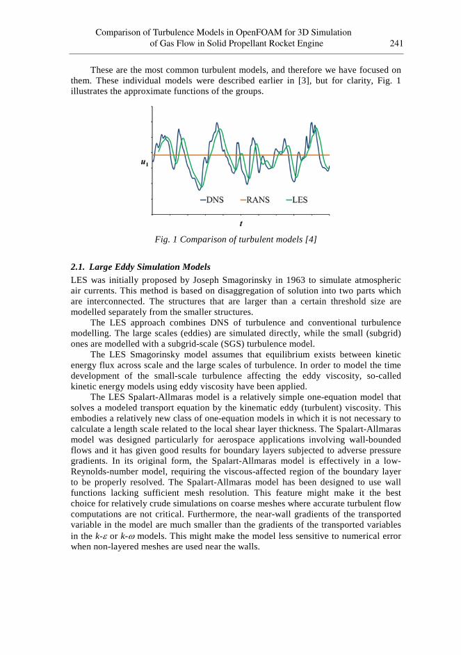
These are the most common turbulent models, and therefore we have focused on them. These individual models were described earlier in [3], but for clarity, Fig. 1 illustrates the approximate functions of the groups.

Fig. 1 Comparison of turbulent models [4]

2.1. Large Eddy Simulation Models LES was initially proposed by Joseph Smagorinsky in 1963 to simulate atmospheric air currents. This method is based on disaggregation of solution into two parts which are interconnected. The structures that are larger than a certain threshold size are modelled separately from the smaller structures.

The LES approach combines DNS of turbulence and conventional turbulence modelling. The large scales (eddies) are simulated directly, while the small (subgrid) ones are modelled with a subgrid-scale (SGS) turbulence model.

The LES Smagorinsky model assumes that equilibrium exists between kinetic energy flux across scale and the large scales of turbulence. In order to model the time development of the small-scale turbulence affecting the eddy viscosity, so-called kinetic energy models using eddy viscosity have been applied.

The LES Spalart-Allmaras model is a relatively simple one-equation model that solves a modeled transport equation by the kinematic eddy (turbulent) viscosity. This embodies a relatively new class of one-equation models in which it is not necessary to calculate a length scale related to the local shear layer thickness. The Spalart-Allmaras model was designed particularly for aerospace applications involving wall-bounded flows and it has given good results for boundary layers subjected to adverse pressure gradients. In its original form, the Spalart-Allmaras model is effectively in a low-Reynolds-number model, requiring the viscous-affected region of the boundary layer to be properly resolved. The Spalart-Allmaras model has been designed to use wall functions lacking sufficient mesh resolution. This feature might make it the best choice for relatively crude simulations on coarse meshes where accurate turbulent flow computations are not critical. Furthermore, the near-wall gradients of the transported variable in the model are much smaller than the gradients of the transported variables in the k-ε or k-ω models. This might make the model less sensitive to numerical error when non-layered meshes are used near the walls.


2.2. Reynolds-Averaged Simulation Models The Reynolds-Averaged Simulation (RAS) is also known as Reynolds-Averaged Navier-Stokes (RANS). The governing equations are solved in the ensemble-averaged form, including appropriate models for the effect of turbulence.

The RANS k-ε model is one of the most common turbulence models. It is a two-equation model that includes two extra transport equations to represent the turbulent properties of the flow. This allows a two-equation model to account for the history effects like convection and diffusion of turbulent energy. The first transported variable is turbulent kinetic energy k. The second transported variable in this case is the turbu-lent dissipation ε. This variable determines the scale of the turbulence, whereas the first variable (k) determines the energy in the turbulence.

The RANS k-ω is also a two-equation model. It includes two extra transport equations to represent the turbulent properties of the flow. The first transported varia-ble is turbulent kinetic energy k. The second transported variable in this case is the specific dissipation ω. This variable determines the scale of the turbulence.

The RANS k-ω SST (Shear-Stress Transport) model is a two-equation turbulence model which solves two transport equations for the kinetic energy k and the specific dissipation ω. The shear stress transport formulation combines the better of two worlds. The use of a k-ω formulation in the inner parts of the boundary layer makes the model directly usable all the way down to the wall through the viscous sub-layer, hence the SST k-ω model can be used as a Low-Re turbulence model without any extra damping functions.

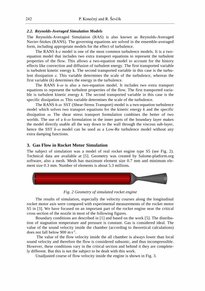
3. Gas Flow in Rocket Motor Simulation The subject of simulation was a model of real rocket engine type S5 (see Fig. 2). Technical data are available at [5]. Geometry was created by Salome-platform.org software, also a mesh. Mesh has maximum element size 0.7 mm and minimum ele-ment size 0.3 mm. Number of elements is about 5.3 millions.

Fig. 2 Geometry of simulated rocket engine

The results of simulation, especially the velocity courses along the longitudinal rocket motor axis were compared with experimental measurements of the rocket motor S5 in [3]. We have focused on an important part of the rocket engine near the critical cross section of the nozzle in most of the following figures.

Boundary conditions are described in [1] and based on the work [5]. The distribu-tion of stagnation temperature and pressure is constant. Gas is considered ideal. The value of the sound velocity inside the chamber (according to theoretical calculations) does not fall below 900 m s-1.

The value of the flow velocity inside the all chamber is always lower than local sound velocity and therefore the flow is considered subsonic, and thus incompressible. However, these conditions vary in the critical section and behind it they are complete-ly different. But this is not the subject to be dealt with this work.

Unadjusted course of flow velocity inside the engine is shown in Fig. 3.


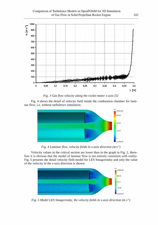
Fig. 3 Gas flow velocity along the rocket motor x-axis [5]

Fig. 4 shows the detail of velocity field inside the combustion chamber for lami-nar flow, i.e. without turbulence simulation.

Fig. 4 Laminar flow, velocity fields in x-axis direction (m s-1)

Velocity values in the critical section are lower than in the graph in Fig. 2, there-fore it is obvious that the model of laminar flow is not entirely consistent with reality. Fig. 5 presents the detail velocity field model for LES Smagorinsky and only the value of the velocity in the x-axis direction is shown.

Fig. 5 Model LES Smagorinsky, the velocity fields in x-axis direction (m s-1)


The difference of laminar flow in Figs. 4 and 5 is clearly visible. Velocity distri-bution around the critical section is different, and the formation of the boundary layer between the main stream and the wall is apparent.

The appearance of the velocity field in Fig. 6 in the z-axis direction (perpendicu-lar to the picture) is almost identical in all models. This suggests that the radial flows are formed within the engine in the way that would be missed in a 2D simulation.

Fig. 6 Model LES Smagorinsky, the velocity fields in z-axis direction (m s-1)

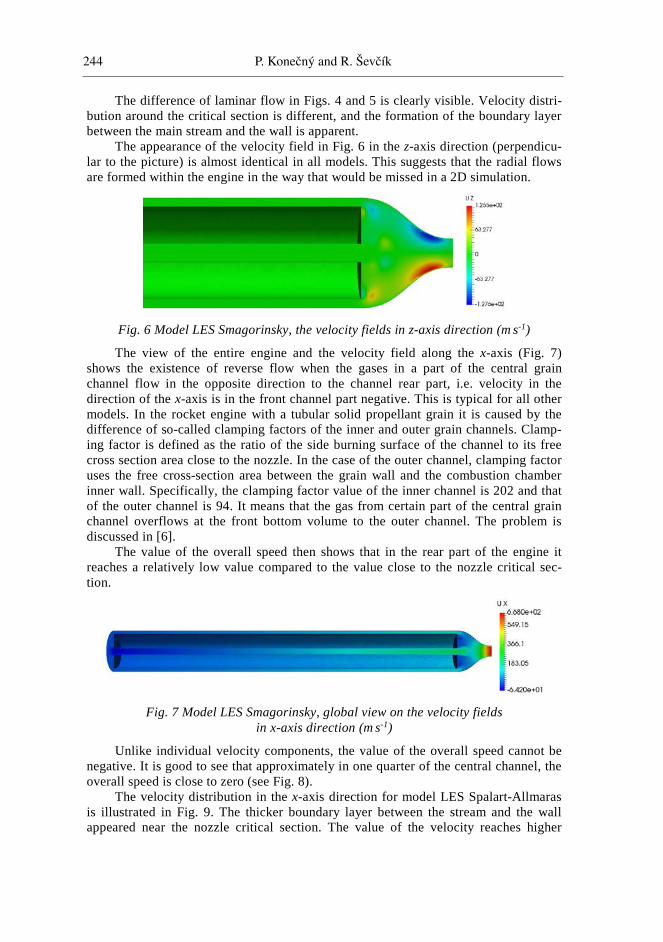
The view of the entire engine and the velocity field along the x-axis (Fig. 7) shows the existence of reverse flow when the gases in a part of the central grain channel flow in the opposite direction to the channel rear part, i.e. velocity in the direction of the x-axis is in the front channel part negative. This is typical for all other models. In the rocket engine with a tubular solid propellant grain it is caused by the difference of so-called clamping factors of the inner and outer grain channels. Clamp-ing factor is defined as the ratio of the side burning surface of the channel to its free cross section area close to the nozzle. In the case of the outer channel, clamping factor uses the free cross-section area between the grain wall and the combustion chamber inner wall. Specifically, the clamping factor value of the inner channel is 202 and that of the outer channel is 94. It means that the gas from certain part of the central grain channel overflows at the front bottom volume to the outer channel. The problem is discussed in [6].

The value of the overall speed then shows that in the rear part of the engine it reaches a relatively low value compared to the value close to the nozzle critical sec-tion.

Fig. 7 Model LES Smagorinsky, global view on the velocity fields

in x-axis direction (m s-1)

Unlike individual velocity components, the value of the overall speed cannot be negative. It is good to see that approximately in one quarter of the central channel, the overall speed is close to zero (see Fig. 8).

The velocity distribution in the x-axis direction for model LES Spalart-Allmaras is illustrated in Fig. 9. The thicker boundary layer between the stream and the wall appeared near the nozzle critical section. The value of the velocity reaches higher


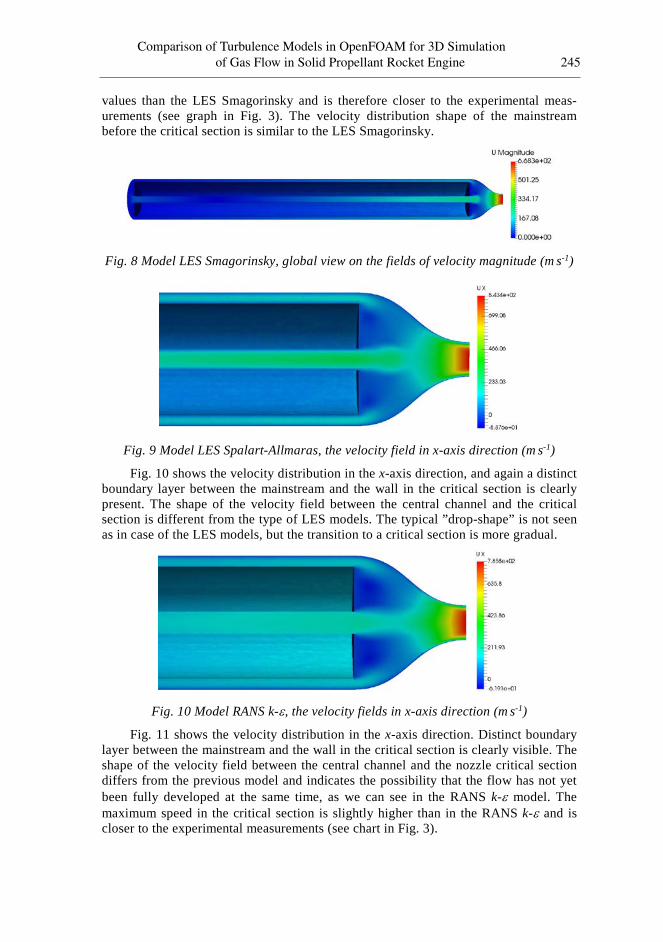
values than the LES Smagorinsky and is therefore closer to the experimental meas-urements (see graph in Fig. 3). The velocity distribution shape of the mainstream before the critical section is similar to the LES Smagorinsky.

Fig. 8 Model LES Smagorinsky, global view on the fields of velocity magnitude (m s-1)

Fig. 9 Model LES Spalart-Allmaras, the velocity field in x-axis direction (m s-1)

Fig. 10 shows the velocity distribution in the x-axis direction, and again a distinct boundary layer between the mainstream and the wall in the critical section is clearly present. The shape of the velocity field between the central channel and the critical section is different from the type of LES models. The typical ”drop-shape” is not seen as in case of the LES models, but the transition to a critical section is more gradual.

Fig. 10 Model RANS k-ε, the velocity fields in x-axis direction (m s-1)

Fig. 11 shows the velocity distribution in the x-axis direction. Distinct boundary layer between the mainstream and the wall in the critical section is clearly visible. The shape of the velocity field between the central channel and the nozzle critical section differs from the previous model and indicates the possibility that the flow has not yet been fully developed at the same time, as we can see in the RANS k-ε model. The maximum speed in the critical section is slightly higher than in the RANS k-ε and is closer to the experimental measurements (see chart in Fig. 3).


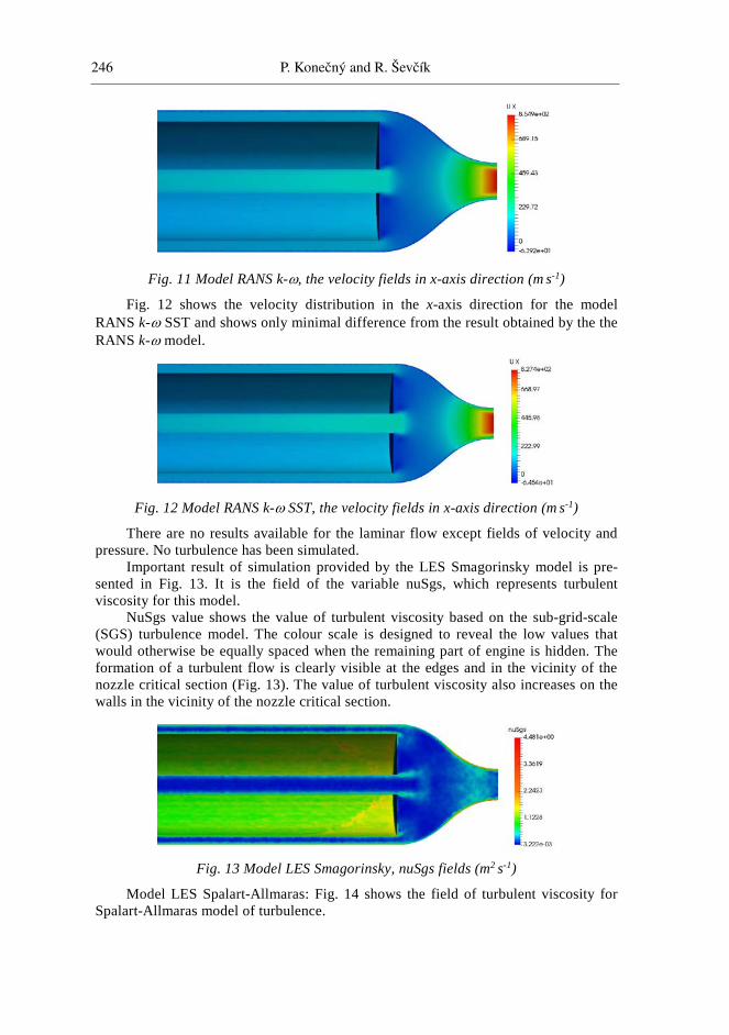
Fig. 11 Model RANS k-ω, the velocity fields in x-axis direction (m s-1)

Fig. 12 shows the velocity distribution in the x-axis direction for the model RANS k-ω SST and shows only minimal difference from the result obtained by the the RANS k-ω model.

Fig. 12 Model RANS k-ω SST, the velocity fields in x-axis direction (m s-1)

There are no results available for the laminar flow except fields of velocity and pressure. No turbulence has been simulated.

Important result of simulation provided by the LES Smagorinsky model is pre-sented in Fig. 13. It is the field of the variable nuSgs, which represents turbulent viscosity for this model.

NuSgs value shows the value of turbulent viscosity based on the sub-grid-scale (SGS) turbulence model. The colour scale is designed to reveal the low values that would otherwise be equally spaced when the remaining part of engine is hidden. The formation of a turbulent flow is clearly visible at the edges and in the vicinity of the nozzle critical section (Fig. 13). The value of turbulent viscosity also increases on the walls in the vicinity of the nozzle critical section.

Fig. 13 Model LES Smagorinsky, nuSgs fields (m2 s-1)

Model LES Spalart-Allmaras: Fig. 14 shows the field of turbulent viscosity for Spalart-Allmaras model of turbulence.


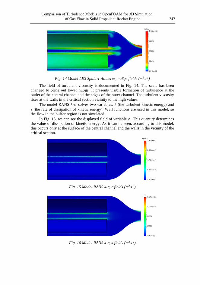
Fig. 14 Model LES Spalart-Allmeras, nuSgs fields (m2 s-1)

The field of turbulent viscosity is documented in Fig. 14. The scale has been changed to bring out lower nuSgs. It presents visible formation of turbulence at the outlet of the central channel and the edges of the outer channel. The turbulent viscosity rises at the walls in the critical section vicinity to the high values.

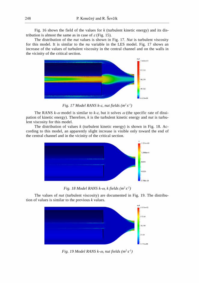
The model RANS k-ε solves two variables: k (the turbulent kinetic energy) and ε (the rate of dissipation of kinetic energy). Wall functions are used in this model, so the flow in the buffer region is not simulated.

In Fig. 15, we can see the displayed field of variable ε . This quantity determines the value of dissipation of kinetic energy. As it can be seen, according to this model, this occurs only at the surface of the central channel and the walls in the vicinity of the critical section.

Fig. 15 Model RANS k-ε, ε fields (m2 s-3)

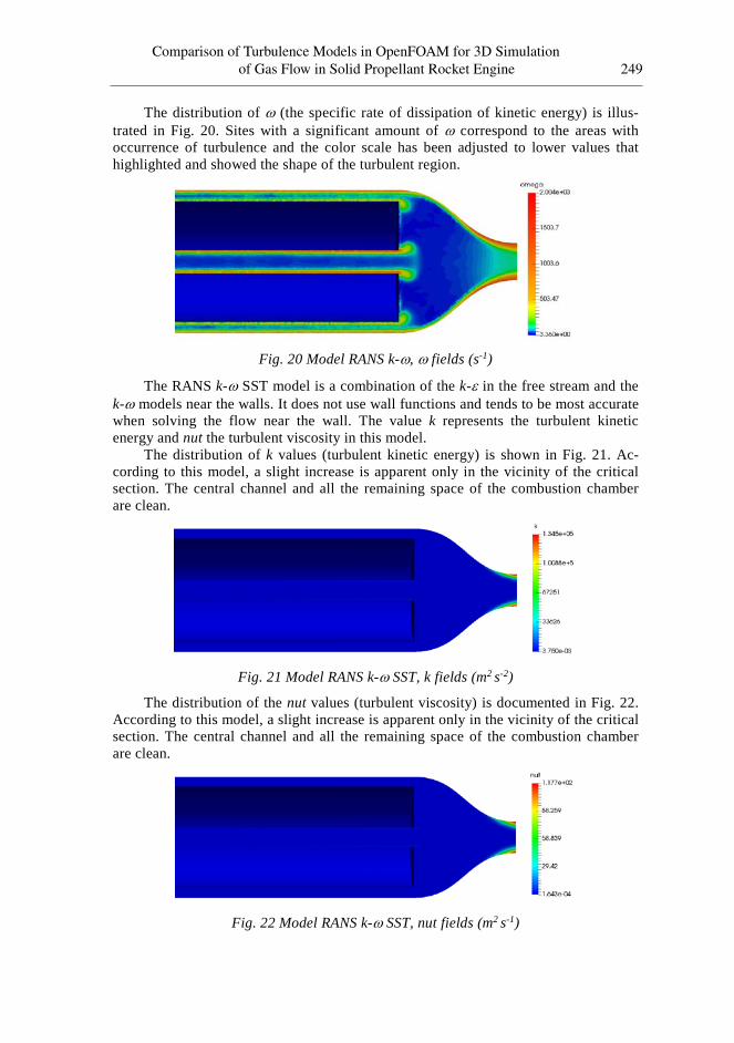
Fig. 16 Model RANS k-ε, k fields (m2 s-2)


Fig. 16 shows the field of the values for k (turbulent kinetic energy) and its dis-tribution is almost the same as in case of ε (Fig. 15).

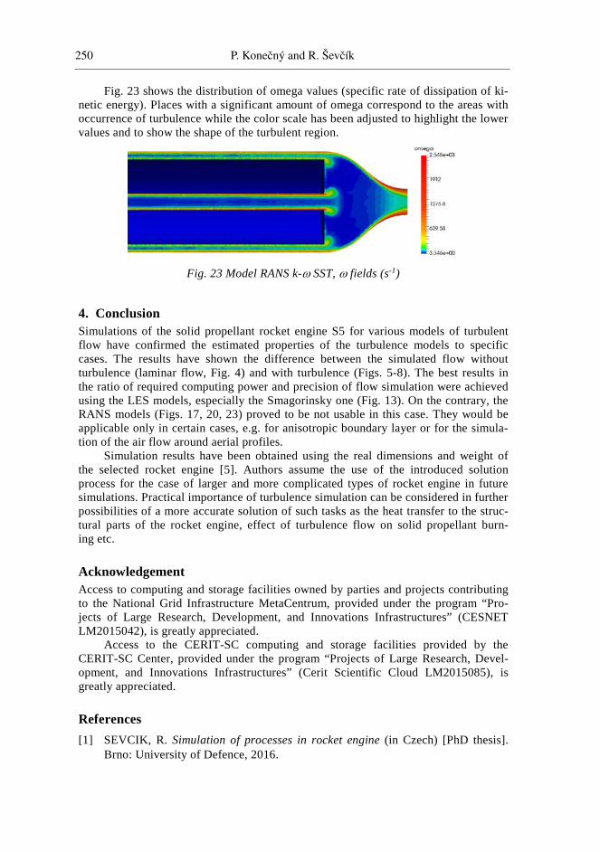
The distribution of the nut values is shown in Fig. 17. Nut is turbulent viscosity for this model. It is similar to the nu variable in the LES model. Fig. 17 shows an increase of the values of turbulent viscosity in the central channel and on the walls in the vicinity of the critical section.

Fig. 17 Model RANS k-ε, nut fields (m2 s-1)

The RANS k-ω model is similar to k-ε, but it solves ω (the specific rate of dissi-pation of kinetic energy). Therefore, k is the turbulent kinetic energy and nut is turbu-lent viscosity for this model.

The distribution of values k (turbulent kinetic energy) is shown in Fig. 18. Ac-cording to this model, an apparently slight increase is visible only toward the end of the central channel and in the vicinity of the critical section.

Fig. 18 Model RANS k-ω, k fields (m2 s-2)

The values of nut (turbulent viscosity) are documented in Fig. 19. The distribu-tion of values is similar to the previous k values.

Fig. 19 Model RANS k-ω, nut fields (m2 s-1)


The distribution of ω (the specific rate of dissipation of kinetic energy) is illus-trated in Fig. 20. Sites with a significant amount of ω correspond to the areas with occurrence of turbulence and the color scale has been adjusted to lower values that highlighted and showed the shape of the turbulent region.

Fig. 20 Model RANS k-ω, ω fields (s-1)

The RANS k-ω SST model is a combination of the k-ε in the free stream and the k-ω models near the walls. It does not use wall functions and tends to be most accurate when solving the flow near the wall. The value k represents the turbulent kinetic energy and nut the turbulent viscosity in this model.

The distribution of k values (turbulent kinetic energy) is shown in Fig. 21. Ac-cording to this model, a slight increase is apparent only in the vicinity of the critical section. The central channel and all the remaining space of the combustion chamber are clean.

Fig. 21 Model RANS k-ω SST, k fields (m2 s-2)

The distribution of the nut values (turbulent viscosity) is documented in Fig. 22. According to this model, a slight increase is apparent only in the vicinity of the critical section. The central channel and all the remaining space of the combustion chamber are clean.

Fig. 22 Model RANS k-ω SST, nut fields (m2 s-1)


Fig. 23 shows the distribution of omega values (specific rate of dissipation of ki-netic energy). Places with a significant amount of omega correspond to the areas with occurrence of turbulence while the color scale has been adjusted to highlight the lower values and to show the shape of the turbulent region.

Fig. 23 Model RANS k-ω SST, ω fields (s-1)

4. Conclusion Simulations of the solid propellant rocket engine S5 for various models of turbulent flow have confirmed the estimated properties of the turbulence models to specific cases. The results have shown the difference between the simulated flow without turbulence (laminar flow, Fig. 4) and with turbulence (Figs. 5-8). The best results in the ratio of required computing power and precision of flow simulation were achieved using the LES models, especially the Smagorinsky one (Fig. 13). On the contrary, the RANS models (Figs. 17, 20, 23) proved to be not usable in this case. They would be applicable only in certain cases, e.g. for anisotropic boundary layer or for the simula-tion of the air flow around aerial profiles.

Simulation results have been obtained using the real dimensions and weight of the selected rocket engine [5]. Authors assume the use of the introduced solution process for the case of larger and more complicated types of rocket engine in future simulations. Practical importance of turbulence simulation can be considered in further possibilities of a more accurate solution of such tasks as the heat transfer to the struc-tural parts of the rocket engine, effect of turbulence flow on solid propellant burn-ing etc.

Acknowledgement Access to computing and storage facilities owned by parties and projects contributing to the National Grid Infrastructure MetaCentrum, provided under the program “Pro-jects of Large Research, Development, and Innovations Infrastructures” (CESNET LM2015042), is greatly appreciated.

Access to the CERIT-SC computing and storage facilities provided by the CERIT-SC Center, provided under the program “Projects of Large Research, Devel-opment, and Innovations Infrastructures” (Cerit Scientific Cloud LM2015085), is greatly appreciated.

References [1] SEVCIK, R. Simulation of processes in rocket engine (in Czech) [PhD thesis].

Brno: University of Defence, 2016.


[2] HOLZINGER, G. OpenFOAM – a Little User-Manual. Linz: Johannes Kepler University, 2015, 251 p.

[3] URUBA, V. Turbulence (in Czech) [Textbook]. Prague: CTU, 2009. [4] VLCEK, P. Turbulent Flow Modelling. In Proceedings of Conference on Pro-

cessing Technology 2013. Prague: CTU, 2013. [5] MYNARIK, P. Influence of Combustion Products of Solid Propellant on the

Course of Processes in the Solid Propellant Rocket Motor (in Czech) [PhD the-sis]. Brno: University of Defence, 2007.

[6] LUDVIK, F. and KONECNY, P. Internal Ballistics of Solid Propellant Rocket Motors (in Czech) [Textboook]. Brno: Military Academy in Brno, 1999, 208 p.

comparison of turbulence models in openfoam for 3d

Documents