comparison of two parametric methods to estimate … of two parametric methods to estimate pesticide...

COMPARISON OF TWO PARAMETRIC METHODS TO ESTIMATEPESTICIDE MASS LOADS IN CALIFORNIA’S CENTRAL VALLEY1

Dina K. Saleh, David L. Lorenz, and Joseph L. Domagalski2

ABSTRACT: Mass loadings were calculated for four pesticides in two watersheds with different land uses in theCentral Valley, California, by using two parametric models: (1) the Seasonal Wave model (SeaWave), in which apulse signal is used to describe the annual cycle of pesticide occurrence in a stream, and (2) the Sine Wavemodel, in which first-order Fourier series sine and cosine terms are used to simulate seasonal mass loading pat-terns. The models were applied to data collected during water years 1997 through 2005. The pesticides modeledwere carbaryl, diazinon, metolachlor, and molinate. Results from the two models show that the ability to captureseasonal variations in pesticide concentrations was affected by pesticide use patterns and the methods by whichpesticides are transported to streams. Estimated seasonal loads compared well with results from previous stud-ies for both models. Loads estimated by the two models did not differ significantly from each other, with theexceptions of carbaryl and molinate during the precipitation season, where loads were affected by applicationpatterns and rainfall. However, in watersheds with variable and intermittent pesticide applications, theSeaWave model is more suitable for use on the basis of its robust capability of describing seasonal variation ofpesticide concentrations.

(KEY TERMS: pesticides; loading; SeaWave; SineWave; modeling; Central Valley.)

Saleh, Dina K., David L. Lorenz, and Joseph L. Domagalski, 2011. Comparison of Two Parametric Methodsto Estimate Pesticide Mass Loads in California’s Central Valley. Journal of the American Water ResourcesAssociation (JAWRA) 47(2):254-264. DOI: 10.1111/j.1752-1688.2010.00506.x

INTRODUCTION

Pesticides are applied in California on a variety ofland use settings including agricultural, urban, andmixed uses. The movement of pesticides into the envi-ronment is affected by many factors. Among the moreimportant are rainfall relative to time of application,the type of irrigation used, land slope, amount andtype of vegetation cover, soil properties (e.g.,

permeability, organic matter content), and physicalproperties of the pesticide. Off-site movement of thesechemicals is a recognized environmental problem.Organophosphate (OP) insecticides are the mostactively managed group of pesticides in the westernUnited States (Zhang et al., 2004). This is due totheir toxicity to aquatic invertebrates (Kuivila andFoe, 1995; de Vlaming et al., 2000), which areimportant prey organisms for fish, and their effecton salmon behavior (Scholz et al., 2000; Sandahl

1Paper No. JAWRA-09-0197-P of the Journal of the American Water Resources Association (JAWRA). Received December 28, 2009;accepted October 5, 2010. ª 2010 American Water Resources Association. This article is a US Government work and is in the public domainin the USA. Discussions are open until six months from print publication.

2Respectively, Hydrologist, U.S. Geological Survey WRD, 6000 J Street, Placer Hall, Sacramento, California 95819; Hydrologist, U.S.Geological Survey WRD, Mounds View, Minnesota 55420; and Research Hydrologist, U.S. Geological Survey WRD, Sacramento, California95819 (E-Mail ⁄ Saleh: [email protected]).

JAWRA 254 JOURNAL OF THE AMERICAN WATER RESOURCES ASSOCIATION

JOURNAL OF THE AMERICAN WATER RESOURCES ASSOCIATION

Vol. 47, No. 2 AMERICAN WATER RESOURCES ASSOCIATION April 2011

et al., 2005). On a state level, a variety of manage-ment efforts, including those related to total maxi-mum daily load (TMDL) plans by the CaliforniaEnvironmental Protection Agency (CalEPA, 2009),were developed to prevent the movement of OP insec-ticides to streams. In 2004, all urban uses of the OPinsecticide diazinon were eliminated (USEPA, 2006).In addition, significant restrictions have been placedon agricultural uses of diazinon, including cancella-tion of its use on many crops, a reduction in applica-tion rates, a reduction in the number of allowableannual applications, and restrictions on the methodsof application.

To adequately assess mass loads, an appropriatemodel must be utilized. A previous study by the U.S.Geological Survey (USGS) National Water QualityAssessment Program (NAWQA) (Domagalski et al.,2008) describes application of the software programLOADEST2, a parametric multivariate regressionmodel that uses a rating-curve method to quantifyloads of pesticide or nutrient in streams. Seasonal dif-ferences in concentrations of agricultural chemicalsin the streams were described using LOADEST2 withfirst-order sine and cosine functions in decimal time[and hereinafter referred to as the Sine Wave model(SineWave)]. Load estimates can be made on anannual, seasonal, or monthly basis (Cohn et al., 1989;Crawford, 1991). Although this model has been usedin a variety of studies and has been successful in pre-dicting mass loads for nutrients, suspended sediment,and dissolved organic carbon (Saleh et al., 2003;Langland et al., 2004; Sprague et al., 2008), there hasbeen limited use of the SineWave model for pesticidesbecause of the abrupt seasonal changes in pesticideconcentrations due to application patterns and diffi-culty in establishing a relationship between concen-trations and stream discharge (Runkel et al., 2004).

More recent studies by Vecchia et al. (2008) andSullivan et al. (2009), describe using the SeasonalWave (SeaWave) model to describe seasonal varia-tions in pesticide concentrations. The SeaWave modelis designed to handle complexities often found in pes-ticide data, such as seasonal variability in concentra-tion caused by pesticide application patterns, therelationship between concentration and streamflow,and the often large number of detections below labo-ratory reporting levels (RLs).

The purpose of this study is to use the SeaWaveand the SineWave models to estimate mass loads offour pesticides (carbaryl, diazinon metolachlor, andmolinate), two of each that were measured in twowatersheds, Arcade Creek and Sacramento River.Results from both models are compared to identifythe more suitable statistical tool to be used when cal-culating loadings of pesticide in watersheds with avariety of land use settings and pesticide use patterns.

The pesticides selected for this study, were used toillustrate different scenarios of pesticide applicationsin the state of California. For this same reason, thetwo watersheds used in this study were selectedbecause they vary in size and land use; Arcade Creek,a relatively small watershed covering an area ofabout 82 km2, with predominant urban land use, andthe Sacramento River, a much larger watershedcovering an area of about 61,700 km2, with a mixtureof land uses.

METHODS

Data Used for Model

Pesticide concentration data processed by Martin(2009) for the two stream-sampling sites were used inthis study to maintain a consistent dataset acrossmultiple applications. Censoring is common in pesti-cide data and refers to a pesticide concentrationreported as less than some value. Censoring occursbecause the analyzing laboratory is unable to detectthe pesticide or quantify its concentration in the sam-ple. The censoring level is set by the laboratory andis based upon analyses of samples into which knownquantities of pesticides have been added. In this arti-cle and for the purpose of comparing pesticide concen-trations in different regions across the nation, theUSGS adopted a uniform method of censoring pesti-cide data. For the data collection period, a consistentminimum RL was determined for each pesticide andset to the maximum long-term method detection level(Martin, 2009). Samples with atypically high RLs dueto sample matrix interference or subpar lab qualityassurance were left as is. The consistent censoringlevel eliminates the possibility of an induced temporalstructure from changes in the censoring level, thusproducing a ‘‘better’’ coefficient for time. That bettertime coefficient for the trend model also means a bet-ter time coefficient for the load model (Martin, 2009).

Concentration data were corrected for analyticalrecovery errors. The NAWQA Program, as part ofits quality control (QC) ⁄ quality assurance plan,requires the spiking of pesticide mixtures into envi-ronmental water samples at a frequency of 5% ofall samples collected. The recoveries of each ana-lyte, as measured by these field spikes, weresmoothed using a 1.5-year moving average (Martinet al., 2009). Concentrations for corresponding timeperiods were adjusted using the smoothed recoveryvalue. Additional details of the recovery correctionmethods are given by Martin (2009) and Martinet al. (2009). In addition to the analysis of pesticide

COMPARISON OF TWO PARAMETRIC METHODS TO ESTIMATE PESTICIDE MASS LOADS IN CALIFORNIA’S CENTRAL VALLEY

JOURNAL OF THE AMERICAN WATER RESOURCES ASSOCIATION 255 JAWRA

recoveries, the dataset was checked for any occur-rences of pesticides in QC blank samples. An exam-ination of the QC data revealed no problems withfalse positive detections.

The period of record, number of detections andnondetections for each site, and reporting limits foreach pesticide are shown in Table 1. Estimates of theamount of pesticides applied in each of these water-sheds were obtained from the California Departmentof Pesticide Regulation (CaDPR, 2009) for the dura-tion of the study (1997-2005). Streamflow data forboth sites were obtained from the USGS NationalWater Information System (NWIS) (http://ca.water.usgs.gov/nwisweb.html).

Mass Load Calculations

Mass loads of pesticides for the period of this study(1997-2005) were calculated by the rating-curvemethod using the two models SineWave and Sea-Wave. Both models were implemented within theS-PLUS statistical software package (TIBCO, 2008).The rating-curve method is a multiple regressionmodel of constituent concentration or load as a func-tion of flow, decimal time, and seasonal variables(Cohn, 2005). Temporal differences of pesticide con-centrations in the streams can be described on sea-sonal bases by aggregating daily load estimates fromthe model over different seasons. In this analysis,two seasons were defined for the time period of thestudy; a precipitation season (October throughMarch), and an irrigation season (April through Sep-tember). Output of both models includes a statisticalsummary, the average daily flux, the variance of theaverage daily flux, and the 95% confidence intervalfor the average daily flux. The uncertainty associatedwith each estimate of mean load is expressed interms of the standard error prediction (SEP), whichrepresents the variability that may be attributed tothe model calibration (parameter uncertainty) (Cohnet al., 1992).

In general terms, a load is an integrated mass fluxover some time interval {ta, tb}:

L ¼Z

lðtÞdt ¼Z

kcðtÞQðtÞdt; ð1Þ

where L is the total load; l is the instantaneous load,for time t; k is a unit conversion factor, for time t; c isthe instantaneous measured concentration, for time t;Q is the instantaneous flow, for time t.

To better compare results obtained from the mod-els, it is important to have an understanding of thespecific form of each model, identifying the differentvariables used in each model to calculate loads.

Sine Wave Model

The general form of the regression equation for theSineWave model is:

lnðCiÞ ¼ b0þb1lnðQiÞþb2½lnðQiÞ�2þb3ðTiÞþb4ðTiÞ2þb5sinð2pTiÞþb6cosð2pTiÞþ ei; ð2Þ

where ln is the natural logarithm function; Ci is thedaily concentration, in micrograms per liter, for dayi; Qi is the measured daily mean flow, in cubic metersper second, for day i; Ti is the time of observation, indecimal years, for day i; b0, …, b6 is the fitted modelcoefficients; and ei is the error for day i.

In practice, the times of observation and the meandaily flows are centered (by subtracting their samplemeans) to reduce colinearity and are described in theexplanatory variables. Loads were derived from thecoefficients obtained from Equation (2). The quadraticterms shown in Equation (2) were dropped when theywere not at a level of significance of 0.05. This modelassumes that concentrations are subject to a seasonalpattern driven by external factors that can bedescribed by a first-order Fourier series (sine andcosine terms) (Runkel et al., 2004). It is important tomention that the SineWave model fits the pesticideconcentrations to a standardized annual sine-cosinesignal and unlike the SeaWave model, it does nottake into account the half-life of the pesticide nordoes it account for multiple applications of thepesticide in the watershed.

TABLE 1. Pesticide Data From Two Watersheds Used for the Model Evaluation in This Study.

Watershed Name Begin Date End Date Pesticide Number of Samples

Arcade Creek 11 ⁄ 26 ⁄ 1996 09 ⁄ 28 ⁄ 2005 Carbaryl RL = 0.03 88 (29)Arcade Creek 11 ⁄ 26 ⁄ 1996 09 ⁄ 28 ⁄ 2005 Diazinon RL = 0.003 88 (0)Sacramento River 11 ⁄ 15 ⁄ 1996 09 ⁄ 28 ⁄ 2005 Metolachlor RL = 0.006 104 (68)Sacramento River 11 ⁄ 15 ⁄ 1996 09 ⁄ 29 ⁄ 2005 Molinate RL = 0.002 93 (25)

Notes: RL, reporting limit, in micrograms per liter. Values in parentheses are number of censored samples (with concentrations below thereporting limit).

SALEH, LORENZ, AND DOMAGALSKI


Seasonal Wave Model

The general form of the regression equation forthis model is:

lnðCiÞ ¼ b0 þ b1lnðQiÞ þ b2½lnðQiÞ�2 þ b3ðTiÞþ b4ðTiÞ2 þ b5WðTiÞ þ ei; ð3Þ

where W is the seasonal wave.As with the SineWave model, the times of observa-

tion and the mean daily flows are centered to reducecolinearity in the explanatory variables. Loads werederived from the coefficients obtained from Equation(3) and the quadratic terms shown in Equation (3)were dropped when they were not significant at a levelof significance of 0.05. The seasonal wave (W) wasimplemented as described by Vecchia et al. (2008),where W describes the annual cycle of pesticide occur-rence in a stream. In general, W is the unique, periodicsolution to the following differential equation:

d

dTWðTÞ ¼ kðTÞ � uWðTÞ; ½0 � T � 1�

kðTÞ ¼X12

k¼1

xkIk� 1

12� T � k

12

� �;

WðT þ jÞ ¼WðTÞ; j ¼ 0;�1;�2; . . .

ð4Þ

where W(T) is the total amount (kilograms) of a par-ticular pesticide in the basin at time T that is avail-able for transport to the stream; k(T) is theinstantaneous input function (kilograms per year); xk

is the instantaneous input rate for the approximatelyone-month interval beginning at monthly time(k ) 1) ⁄ 12; by convention, the rates are relative rates

scaled from 0 to 1; u is the decay rate that controlsthe rate at which pesticides are removed from thestream system; and I is the indicator function withI (a £ t < b) = 1, if t lies in the given interval, andI (a £ t < b) = 0 otherwise.

The function W depends on two parameters,x = {x1, …, x12} and u as included in Equation (4).Parameter u condenses various important transportprocesses such as sorption, microbial degradation andmineralization, photodegradation, plant uptake, vola-tilization, and soil slope and permeability into a sin-gle value useful in describing the retention andmobility of the pesticide in the watershed beingmodeled. The value of (12 ⁄ u = h) approximates thehalf-life (in months) of the pesticide in the watershedand is the value that is typically used to specify u(Vecchia et al., 2008). The values considered for uand x for this study are shown in Table 2.

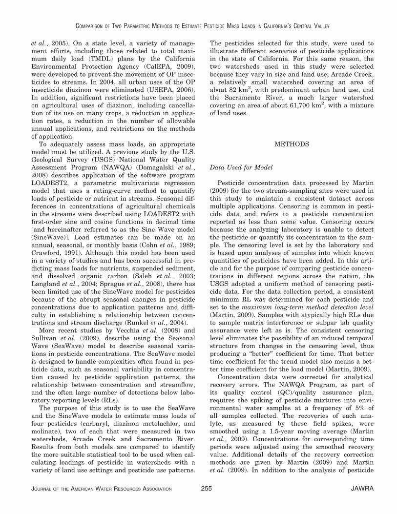
Equation (4) was applied to the two streamsfor each of the four selected pesticides. Unlike thestandardized fitted sine-cosine signal of the Sine-Wave model, the SeaWave model output of thisfunction provides a list of multiple forms of W withthe x and h values corresponding to each modelaccompanied with an Akaike Information Criterion(AIC) value for each model (Akaike, 1981). The bestchoice for W for each site was determined using thehighest AIC value. Figure 1 shows a composite sea-sonal wave W superimposed upon the pesticide con-centration data and streamflow in the differentwatersheds. The magnitude, shape, and peak loca-tion of W varies for these four pesticides (Figure 1).It is affected by the amount and time periodin which pesticides are applied and removed in thedifferent watersheds. In some cases, W has one peak(Figure 1C). This indicates that in the Sacramento

TABLE 2. Model Choices for Describing Seasonal Variation of Pesticides Application Rates (equation 3).

Model Number h = 12 ⁄ u x1 x2 x3 x4 x5 x6 x7 x8 x9 x10 x11 x12

1 1, 2, 3, 4 0 0 0 0 0 1 0 0 0 0 0 02 1, 2, 3, 4 0 0 0 0 0 1 1 0 0 0 0 03 1, 2, 3, 4 0 0 0 0 0 1 1 1 0 0 0 04 1, 2, 3, 4 0 0 0 0 0 1 1 1 1 0 0 05 1, 2, 3, 4 0 0 0 0 1 1 1 1 1 0 0 06 1, 2, 3, 4 1 1 1 1 1 1 1 1 1 0 0 071 1, 2, 3, 4 0 0 1 1 1 0 0 0 1 0 0 08 1, 2, 3, 4 0 0 1 1 1 0 0 0 0 1 0 09 1, 2, 3, 4 0 0 1 1 1 0 0 0 0 0 1 0

10 1, 2, 3, 4 0 0 1 1 1 0 0 0 0 0 0 111 1, 2, 3, 4 0 0 1 1 1 0 0 0.752 0.75 0 0 012 1, 2, 3, 4 0 0 1 1 1 0 0 0 0.75 0.75 0 013 1, 2, 3, 4 0 0 1 1 1 0 0 0 0 0.75 0.75 014 1, 2, 3, 4 0 0 1 1 1 0 0 0 0 0 0.75 0.75

1In the two peak Wave model, the primary peak application rate is always three months.2The secondary peak application rate is lower (0.75) but lasts for a longer time period (two months).



River watershed, metolachlor was being applied, ortransported to the stream, once during the year withthe main application and transport occurring duringthe late spring (Figure 2C). The rate of decrease ofW is related to the half-life of the pesticides in thewatershed. In this case, metolachlor has a smallhalf-life (h = 1) and is removed from the watershedwithin a few months (Figure 1C). In a different sce-nario, molinate in the Sacramento River watershedis applied on rice fields once a year in late spring.Water in rice fields is managed according to stateregulations, where the water must be held for at

least 28 days before it can be released (Newhart,2002). The fields are flooded in late April and earlyMay, when molinate is applied (Figure 2D). Some ofthe initially applied water, containing pesticide resi-dues is released in late May which accounts for thepeak in molinate concentrations shown in Figure 1D.Released water is then replaced with new waterallowing diluted concentrations of molinate toremain in the rice fields for a longer time period(h = 3). This is illustrated in a wide single peak sea-sonal wave W form shown in Figure 1D.

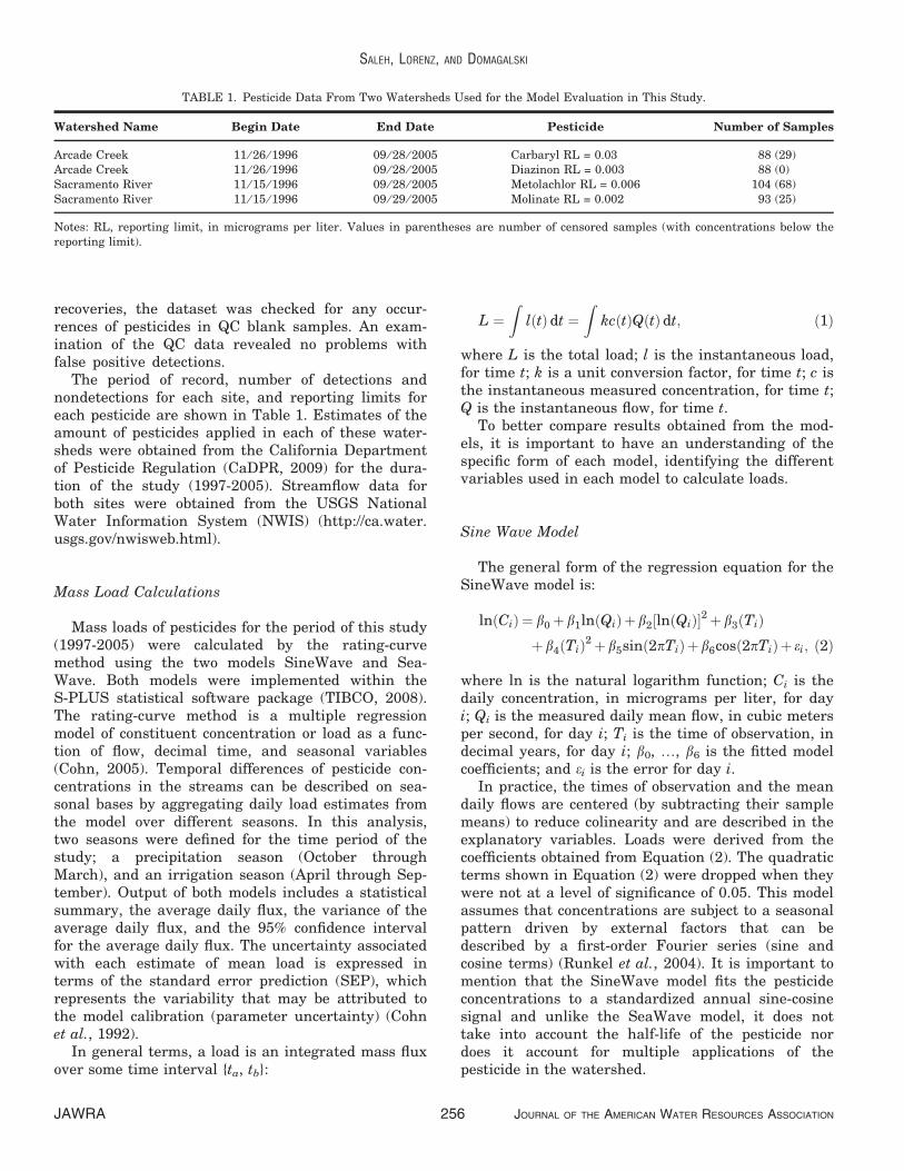
It is possible for W to have a double peak(Figure 1A), which indicates that in this watershedthere are multiple applications or processes thattransport pesticides to the stream. For example,carbaryl in the Arcade Creek watershed is appliedtwice in the year – once in the spring (March andApril) with the presence of precipitation as a maintransport mechanism of pesticides to the stream anda second application of less magnitude during thesummer (June through August) when irrigation isthe main transport mechanism (Figure 2A). Figure 1Areflects this multiple pesticide application and trans-port. The seasonal W shown in Figure 1A has ax = 12 and an h = 4 that represents a two peak wavewith a long half-life (Table 2). The pattern of pesticideoccurrence does not always correspond to the season-ality function W. For example, Figure 2B shows thatdiazinon is applied throughout the year, which isreflected in the relatively small seasonal variationwith no distinct peaks in concentration shown inFigure 1B.

It is important to note that for multiple years ofdata, and potentially different application times, ortransport to the river because of different hydrologicconditions, the timing of the major peak of the finaldefined sine and cosine wave, as well as the compos-ite W for the entire time period (1997 to 2005), mightbe slightly shifted from the true location for anygiven year (Vecchia et al., 2008).

The Empirical Correlogram

One of the assumptions of linear regression is thatresiduals are independent. Serial correlation may beexhibited for data collected over time, such as constit-uents in water, which violates the assumption ofindependence (Helsel and Hirsch, 2002). Time-seriesmethods easily address data that are spaced uni-formly, but are not easily applied to data collected atvarying time intervals. The empirical correlogramdescribed in this section is a method to portray anddiagnose potential serial correlation in data collectedat varying time intervals. The correlogram willeffectively show a distinct periodic signal rather than

Seasonality Function, WStream flowConcentrationsnondetects

Car

bary

l Con

cent

ratio

n,

in m

icro

gram

s pe

r lite

r

0.01

1.0

0.1SeaWave Model (12,4)A

0.01 0.0

0.5

1.0

1.5

2.0

1.0

0.1SeaWave Model (5,4)B

100

500

900

13001.0

0.1

0.01

0.1 0.3 0.5 0.7 0.9

SeaWave Model (1,3)D

Decimal Time, Month

SeaWave Model (3,1)0.1

0.01

C

0.0

0.5

1.0

1.5

2.0

100

500

900

1300

Dia

zino

n C

once

ntra

tion,

in

mic

rogr

ams

per l

iter

Met

olac

hlor

Con

cent

ratio

n,

in m

icro

gram

s pe

r lite

rM

olin

ate

Con

cent

ratio

n,

in m

icro

gram

s pe

r lite

r

FIGURE 1. The Composite Seasonal Wave Form (W) for the EntireTime Period of Study, 1997 to 2005. Values in parentheses are xand u, respectively, used for the model simulation. (A) Best-fitmodel for seasonal wave pulse for carbaryl in Arcade Creek.(B) Best-fit model for seasonal wave pulse for diazinon in ArcadeCreek. (C) Best-fit model for seasonal wave pulse for metolachlor inthe Sacramento River. (D) Best-fit model for seasonal wave pulsefor molinate in the Sacramento River.



a time-varying signal that can be evident in thetime-series plot. In traditional time-series analysis,for a discrete set of equally spaced observations {x1,x2, …, xN}, the correlation between observations forany discrete difference in time, rk, can be computedas,

rk ¼

PN�k

j¼1

xj � �x� �

xjþk � �x� �

PNj¼1

xj � �x� �2

; ð5Þ

where N is the number of observations, xj is theobservation at a discrete time j, and �x is the mean ofall observations (Chattfield, 1980). To define theresidual empirical correlogram, let

xj ¼ etðjÞ; j ¼ 1; 2; . . . ;N

denote the residual from regression model (1) or (2),where t(j) is the time (in Julian day) of the jthobservation. Also let

djk ¼ tðkÞ � tðjÞ

be the difference between the jth and the kthsampling time and define the standardized residualcross-product for each pair of observations,

cjk¼ðxj��xÞðxk��xÞ1N

PNe¼1 xe��xð Þ

;j¼1;...;N;k¼j¼1;...;N: ð6Þ

The residual empirical correlogram for a given timelag, Dt, is obtained by applying a kernel smoothing

0

500

1,000

1,500

2,000

2,500

0

2,000

4,000

6,000

8,000

10,000

12,000

01 02 03 04 05 06 07 08 09 10 11 12

A

B

Date, in Month

0

50,000

100,000

150,000

200,000

250,000

300,000

Carbaryl Applied

Diazinon Applied

Molinate AppliedD

Car

bar

yl A

pp

lied,

kg

/mo

nth

Dia

zin

on

Ap

plie

d, k

g/m

on

thM

olin

ate

Ap

plie

d, k

g/m

on

th

0

1,000

2,000

3,000

4,000

5,000

6,000

7,000C Metolachlor, S-Metolachlor Applied

Met

ola

chlo

r Ap

plie

d, k

g/m

on

th

FIGURE 2. Pesticide Use Data Obtained From the California Department of Pesticide Regulation, in Average Kilograms of PesticidesApplied Per-Month, 1997 to 2005. (A) Carbaryl applied in the Arcade Creek watershed. (B) Diazinon applied in the Arcade Creek watershed.

(C) Metolachlor applied in the Sacramento River watershed. (D) Molinate applied in the Sacramento River watershed.



function to the standardized cross-products, where thecross-products with djk close to Dt receive more weightthan those with djk far from Dt,

rDt ¼

PNj¼1

PNk¼jþ1

K djk � Dt� �

cjk

PNj¼1

PNk¼jþ1

K djk � Dt� � ; ð7Þ

where

KðuÞ ¼ 1 jujc ; juj � c

0; juj>c

�

and u is the difference between the two lag times(j, k).

The function K, used to calculate weights for thecorrelogram, is called a triangle kernel functionbecause the weighting scheme is shaped like a trian-gle, and is scaled by c so that half the area of thetriangle is between )0.25 and 0.25 (TIBCO, 2008).The scaling factor is about 0.854. For censored data,the deviance residual is used as an approximation forthe actual value. The standardized residual cross-product is plotted against the difference in time forall points where Dt is >0. This approach assumes thatthe very short-term random fluctuations in sampledvalues are large enough that there is an almostimmediate change in the correlation from 0.0 to thecomputed value at some small increment in time. Ifthe residuals contain a seasonal fluctuation due tolack of fit, then the correlogram will exhibit an oscil-lation at the same frequency (Chattfield, 1980).

RESULTS

Statistical Analyses

There are two main factors affecting the presenceand concentration of pesticides in the streams; theamount of pesticides applied in the watershed (dataavailable from CaDPR, 2009), and the manner inwhich these pesticides are transported throughoutthe system (runoff following precipitation or irriga-tion, and groundwater transport). In this study,carbaryl has two main application periods in theurbanized Arcade Creek watershed, the first inspring (March through April) and the second insummer (June through August) (Figure 2A). Duringthe first application period, spring rainstorms stilloccur, but during the second application period thereis little rainfall but extensive landscape irrigation. Itappears that the transport of carbaryl is more likely

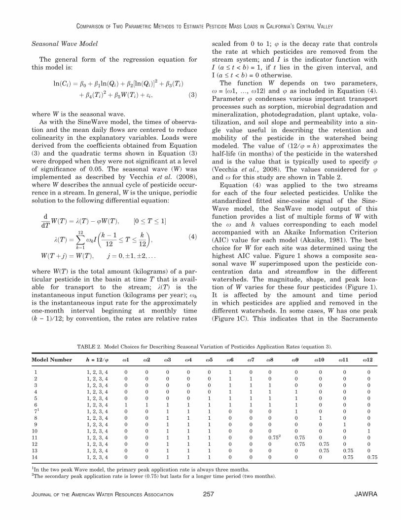
to occur as a result of rain rather than irrigation, asthe largest modeled peak occurs during the firstapplication period corresponding with high flows inArcade Creek (Figure 1A). These multiple applica-tions allow carbaryl to remain in the watershed fora long time period (Figure 1A). Figures 3A and 3Bshow the residual empirical correlogram plotted overa lag time of one and a half years, using both Sea-Wave and SineWave, respectively. Figure 3B showsthat there are two well-defined periods when Sine-Wave overestimated values, and two periods whenSineWave underestimated values. This is reflected ina well-defined cyclical kernel smooth-line pattern,with two peaks per year shown in Figure 3B. On theother hand, the SeaWave model provides a betterestimate of values throughout the year and this isreflected in a flat kernel smooth-line pattern shownin Figure 3A. Residual variance values obtainedfrom both models also indicate that SeaWave wasmore successful in capturing the seasonal occurrencefor carbaryl in the Arcade Creek watershed(Table 3).

Diazinon, an insecticide, was applied at varioustimes throughout the year in the Arcade Creekwatershed throughout the duration of the study(Figure 2B). In 2004, all urban uses of diazinon wereeliminated nationwide because of the effect of diazi-non on human health (USEPA, 2006). In addition,watershed management TMDL plans were institutedin agricultural areas to reduce diazinon toxicity toaquatic invertebrates. Figures 3C and 3D show theresidual empirical correlogram plots for diazinon inArcade Creek using both SeaWave and SineWave,respectively. The empirical correlograms show noseasonal variation because both models predicted theseasonality (or in this case, lack of seasonality) well,leaving no seasonal structure in the residuals(Figures 3C and 3D).

In the Sacramento River watershed, the herbicidemetolachlor is applied during late spring and earlysummer while spring rainstorms still occur. Given thehigh flows in the Sacramento River, and single applica-tion on crops, metolachlor is removed from thewatershed in a relatively short time period (Figure 1C).The residual empirical correlogram plots from the Sea-Wave and SineWave models for metolachlor at the Sac-ramento River site shown in Figures 3E and 3Frespectively indicate that both models were equallysuccessful in capturing the seasonal occurrence patternfor metolachlor in the watershed. This is reflected in aflat kernel smooth line shown in Figures 3E and 3F.

It was expected that maximum concentrations ofmolinate would occur in the May to June time framewith decreasing concentrations after that. The ini-tially applied irrigation water cannot be held on thefield for the entire growing season because it causes



problems with the crop and therefore, the farmersrelease some water periodically and flood with newirrigation water, thus gradually diluting the molinateconcentrations till it is completely removed from thewatershed in the late summer. Figures 3G and 3Hshow residual empirical correlogram plots for moli-nate. Figure 3H shows that the SineWave model wasunsuccessful in capturing the seasonal variability ofmolinate concentrations in the watershed. This isreflected in a well-defined cyclical kernel smooth-linepattern shown in Figure 3H. On the other hand,the SeaWave model better captured the seasonal

variability as indicated by a flat kernel smooth lineshown in Figure 3.

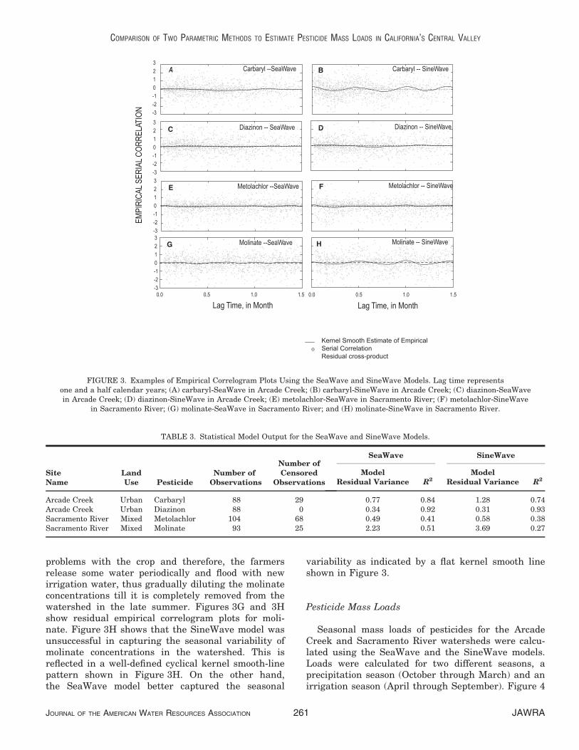
Pesticide Mass Loads

Seasonal mass loads of pesticides for the ArcadeCreek and Sacramento River watersheds were calcu-lated using the SeaWave and the SineWave models.Loads were calculated for two different seasons, aprecipitation season (October through March) and anirrigation season (April through September). Figure 4

EMPI

RICA

L SER

IAL C

ORRE

LATI

ON -3-2-10123

Carbaryl -- SineWaveA

Kernel Smooth Estimate of Empirical Serial CorrelationResidual cross-product

-3-2-10123

Carbaryl --SeaWave B

0.0 0.5 1.0 1.50.0 0.5 1.0 1.5

Metolachlor -- SineWaveMetolachlor --SeaWaveE F

Lag Time, in Month Lag Time, in Month

-3-2-10123

Diazinon -- SineWaveDiazinon -- SeaWaveC D

Molinate --SeaWaveG

-3-2-10123

H Molinate -- SineWave

FIGURE 3. Examples of Empirical Correlogram Plots Using the SeaWave and SineWave Models. Lag time representsone and a half calendar years; (A) carbaryl-SeaWave in Arcade Creek; (B) carbaryl-SineWave in Arcade Creek; (C) diazinon-SeaWavein Arcade Creek; (D) diazinon-SineWave in Arcade Creek; (E) metolachlor-SeaWave in Sacramento River; (F) metolachlor-SineWave

in Sacramento River; (G) molinate-SeaWave in Sacramento River; and (H) molinate-SineWave in Sacramento River.

TABLE 3. Statistical Model Output for the SeaWave and SineWave Models.

SiteName

LandUse Pesticide

Number ofObservations

Number ofCensored

Observations

SeaWave SineWave

ModelResidual Variance R2

ModelResidual Variance R2

Arcade Creek Urban Carbaryl 88 29 0.77 0.84 1.28 0.74Arcade Creek Urban Diazinon 88 0 0.34 0.92 0.31 0.93Sacramento River Mixed Metolachlor 104 68 0.49 0.41 0.58 0.38Sacramento River Mixed Molinate 93 25 2.23 0.51 3.69 0.27



is a graphical representation of model output display-ing the differences between the results of the twomodels. Traditional methods used to compare pairedobservations, either the paired t-test or the Wilcoxonsigned-rank test, are not appropriate for these databecause the seasonal loads are not independent –they are computed from regression models based onthe same calibration data and estimated from thesame daily flow data. Also, the t-test is very sensitiveto constant small differences in model output,therefore an approximation statistic method, theModel Percent Difference (MPD), was used to evalu-ate differences in model output. This method is notas sensitive as the t-test to constant small differencesin model output.

The MPD value is defined as:

MPD ¼ 200

� ðLSeaWave � LSineWaveÞ=ðLSeaWave þ LSineWaveÞ%SEP

� �ð8Þ

LSeaWave is the load calculated using the SeaWavemodel; LSineWave is the load calculated using the Sine-Wave model; %SEP is the mean percent standarderror of prediction for both SeaWave and SineWave.

For a single observation, the statistic would beexpected to be within )2.0 to 2.0 about 95% of the

time. For eight observations (representing eight yearsof simulation), the same approximate 95% confidencelimits are )2.0 ⁄ 81 ⁄ 2 to 2.0 ⁄ 81 ⁄ 2 or about )0.7 to 0.7.For this study, the comparison between the seasonalloads for the SeaWave and the SineWave modelswere classified as substantially different if MPD were>0.7 and not substantially different if MPD were<0.7. Figure 4 shows that during the precipitationseason, the SeaWave and SineWave models are sta-tistically different only for calculated loads for carba-ryl in the Arcade Creek and molinate in theSacramento River watersheds, where the MPD asso-ciated with the loads are significant >0.7. On theother hand, during the irrigation season the modelsare statistically comparable for all pesticides in thetwo watersheds where MPD is <0.7. These resultsare related to the shape of the seasonal wave for Wused to simulate the occurrence of these different pes-ticides in the two watersheds. In general, when thewidth of W is greater than the width of one-half ofthe wavelength of the fitted sine-cosine signals, thenthe estimated loading value obtained from the Sine-Wave and SeaWave models are significantly differentand MPD is >0.7. This is illustrated in Figures 1Aand 1D, where W for carbaryl and molinate has alarge half-life (h = 4 and 3 respectively). On the con-trary, when the width of W is less than the width ofone-half of the wavelength of the sine-cosine signal

EXPLANATION 90th percentile

75th percentilemedian25th percentile10th percentile

SineWaveSeaWave

Carb

aryl

Load

s, in

gram

s per

seas

on

A

Metol

achlo

r Loa

ds, in

gram

s per

seas

on

Irrigation Season

C

Precipitation Season

Diaz

inon L

oads

, in gr

ams p

er se

ason

B

1000

500

100Mo

linate

Load

s, in

kilog

rams

per s

easo

n

Irrigation Season

D

Precipitation Season

100

500

5,000

1,000

50100

1,000

10,000

3,000

4,000

5,000

10,000

MPD = 0.51 MPD = 0.90 MPD = 0.59 MPD = 0.04

MPD = 0.18 MPD = 1.02

MPD = 0.00

MPD = 0.15

FIGURE 4. Box Plots Showing Seasonal Loads Computed Using the SeaWave and the SineWave Modelsfor an Irrigation Season (April-September) and a Precipitation Season (October-March). Model Percent Difference (MPD)

is indicated and a value >0.7 indicates that the two models are significantly different. (A) Carbaryl at Arcade Creek;(B) diazinon at Arcade Creek; (C) metolachlor at Sacramento River; and (D) molinate at Sacramento River.



then the estimated loading value obtained from theSineWave and SeaWave models are similar and MPDis <0.7 (Figure 1C, h = 1 for metolachlor).

SUMMARY AND CONCLUSIONS

The occurrence of pesticides in streams is greatlyaffected by the amount of pesticide use, the applica-tion pattern in the watershed, and the way pesticidesare transported to streams. In this study, mass loadsfor four pesticides (carbaryl, diazinon, metolachlor,and molinate) in two watersheds with different sizeand land uses (Arcade Creek; small with urban landuse, and Sacramento River; large with mixed landuses) were calculated using the SeaWave and theSineWave models. Results of the two models werecompared in an attempt to identify the most usefultool for analyzing pesticide concentration data underdifferent application conditions.

Results for this study are affected by the ability ofthe SineWave and SeaWave models to capture theseasonal variation of pesticides concentrations in thewatersheds. Unlike the SineWave model, where astandardized sine-cosine signal is applied to simulatepesticides concentrations, the SeaWave model outputprovides a list of multiple forms of a seasonal wave(W) to account for the variability in pesticide concen-trations in the watersheds. In this study, the fourpesticides represent four different application andtransport patterns.

The first example was carbaryl in the ArcadeCreek watershed. This insecticide is applied twice ayear, in spring and summer. The transport of carba-ryl is mostly affected by precipitation. Results showthat the SeaWave model was more successful thanthe SineWave in capturing the seasonal variability incarbaryl occurrence in the Arcade Creek watershedcaused by the multiple application of carbaryl in thewatershed. As a result and during the precipitationseason (October through March) when the flows inArcade Creek are high, the calculated loads from theSeaWave and SineWave models were substantiallydifferent with a MPD >0.7.

The second example was that of diazinon in theurbanized Arcade Creek watershed. Diazinon wasapplied repeatedly throughout the year, which meansthat there was no seasonal variability in diazinonconcentrations in the Arcade Creek. This wasreflected in the inability of the SeaWave model todefine a strong application peak wave form W for thispesticide. As a result, both models predicted the sea-sonality (or in this case, lack of seasonality) well,leaving no seasonal structure in the residuals.

The third example was that of metolachlor in theSacramento River watershed. Metolachlor is appliedin the late spring ⁄ early summer. It has a short half-life and is removed from the system by the end of thesummer. Results show that both models simulatedthe peak in metolachlor concentration well – thewidth of the SeaWave form W is smaller than thewidth of one-half the wavelength of the sine-cosinesignal fitted by the SineWave model. Calculated loadsfrom both models when compared statistically showthat results are not substantially different with aMPD <0.7.

The final example was molinate in the SacramentoRiver watershed. This herbicide is applied in latespring on rice fields, which are highly controlled flowsystems. The rice fields are flooded in late April toearly May and molinate is applied. Some of this ini-tial water is then removed in late May and replacedwith new water allowing the molinate to remain onthe fields but in diluted concentrations till the wateris fully drained from the fields in the late summer.By fitting the sine-cosine signal to the data, the Sine-Wave model was unsuccessful in capturing seasonalvariability of molinate concentrations. This is reflectedin a well-defined cyclical kernel smooth-line patternfitted to the SineWave model residuals. On the otherhand, the SeaWave was successful in simulating sea-sonal variability in molinate concentrations causedby the variability in pesticides transport by fitting asuitable seasonal W form to the data.

On the basis of these results, in watersheds withvariable and intermittent pesticide applications, theSeaWave model would be more suitable to use, due toits robust capability of describing seasonal variationof pesticides concentrations in the watershed.

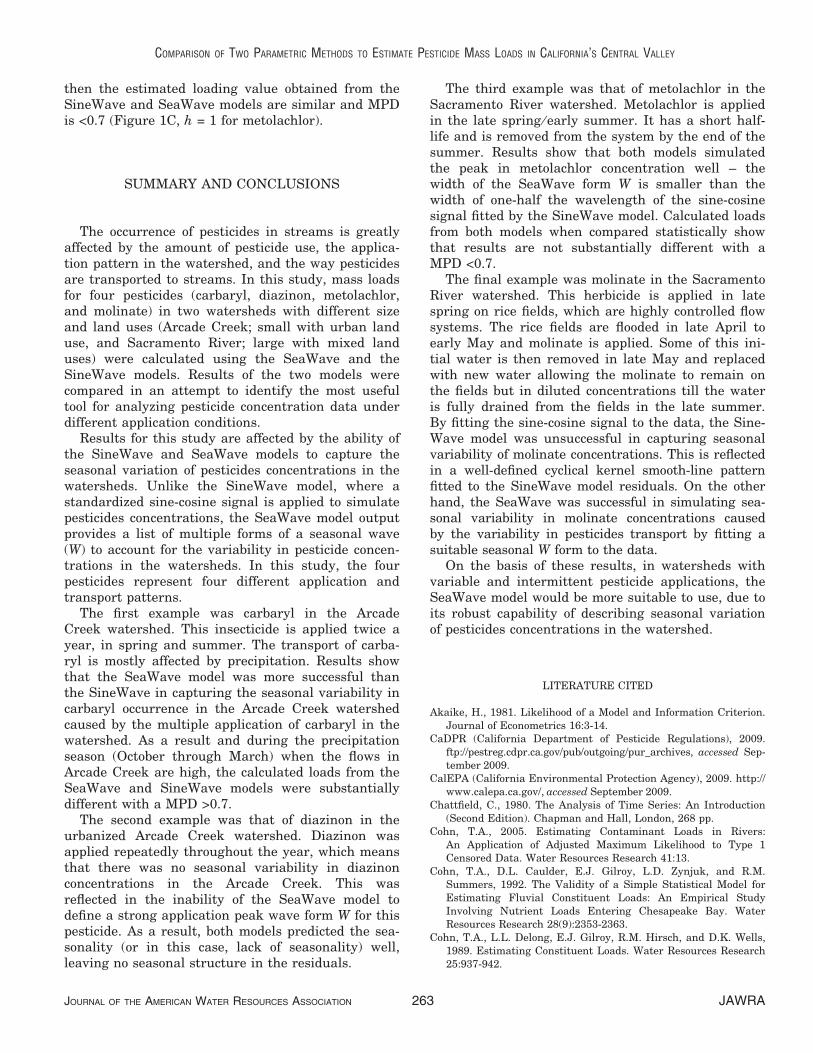
LITERATURE CITED

Akaike, H., 1981. Likelihood of a Model and Information Criterion.Journal of Econometrics 16:3-14.

CaDPR (California Department of Pesticide Regulations), 2009.ftp://pestreg.cdpr.ca.gov/pub/outgoing/pur_archives, accessed Sep-tember 2009.

CalEPA (California Environmental Protection Agency), 2009. http://www.calepa.ca.gov/, accessed September 2009.

Chattfield, C., 1980. The Analysis of Time Series: An Introduction(Second Edition). Chapman and Hall, London, 268 pp.

Cohn, T.A., 2005. Estimating Contaminant Loads in Rivers:An Application of Adjusted Maximum Likelihood to Type 1Censored Data. Water Resources Research 41:13.

Cohn, T.A., D.L. Caulder, E.J. Gilroy, L.D. Zynjuk, and R.M.Summers, 1992. The Validity of a Simple Statistical Model forEstimating Fluvial Constituent Loads: An Empirical StudyInvolving Nutrient Loads Entering Chesapeake Bay. WaterResources Research 28(9):2353-2363.

Cohn, T.A., L.L. Delong, E.J. Gilroy, R.M. Hirsch, and D.K. Wells,1989. Estimating Constituent Loads. Water Resources Research25:937-942.



Crawford, C.G., 1991. Estimation of Suspended-Sediment RatingCurves and Mean Suspended-Sediment Loads. Journal ofHydrology 129:331-348.

Domagalski, J.L., S.W. Ator, R. Coupe, K. McCarthy, D. Lampe,M. Sandstrom, and N. Baker, 2008. Comparative Study ofTransport Processes of Nitrogen, Phosphorus, and Herbicides toStreams in Five Agricultural Basins, USA. Journal of Environ-mental Quality 37:1158-1169.

Helsel, D.R. and R.M. Hirsch, 2002. Statistical Methods in WaterResources. U.S. Geological Survey Techniques of WaterResources Investigation Book 4, Chapter A3, Elsevier, NewYork, 523 pp.

Kuivila, K.M. and C.G. Foe, 1995. Concentrations, Transport,and Biological Effects of Dormant Spray Pesticides in the SanFrancisco Estuary, California. Environmental Toxicology andChemistry 14(7):1141-1150.

Langland, M.J., S.W. Phillips, J.P. Raffensperger, and D.L. Moyer,2004. Changes in Stream Flow and Water Quality in SelectedNontidal Sites in the Chesapeake Bay Basin, 1985-2003.Scientific Investigations Report 2004-5259, USGS, Reston,Virginia, 50 pp.

Martin, J.D., 2009. Sources and Preparation of Data for AssessingTrends in Concentrations of Pesticides in Streams of the UnitedStates, 1992-2006. U.S. Geological Survey Scientific Investiga-tions Report 2009-5062, 50 pp.

Martin, J.D., W.W. Stone, D.S. Wydoski, and M.W. Sandstrom,2009. Adjustment of Pesticide Concentrations for TemporalChanges in Analytical Recovery, 1992-2006. U.S. GeologicalSurvey Scientific Investigations Report 2009-5189, 33 pp.

Newhart, K.L., 2002. Rice Pesticide Use and Surface WaterMonitoring 2002. California Regional Water Quality ControlBoard, Sacramento, California, 36 pp. http://www.cdpr.ca.gov/docs/emon/pubs/ehapreps/eh0209/eh0209.pdf, accessed September2009.

Runkel, R.L., C.G. Crawford, and T.A. Cohn, 2004. Load Estimator(LOADEST) – a FORTRAN Program for Estimating ConstituentLoads in Streams and Rivers. U.S. Geological Survey Tech-niques and Methods, 4-A5, 69 pp.

Saleh, D.K., J.L. Domagalski, C.R. Kratzer, and D.L. Knifong,2003. Organic Carbon Trends, Loads, and Yields to the Sacra-mento-San Joaquin Delta, California, Water Years 1980 to2000. U.S. Geological Survey Water-Resources InvestigationsReport 2003-4070, Reston, Virginia, 77 pp.

Sandahl, J.F., D.H. Baldwin, J.J. Jenkins, and N.L. Scholz, 2005.Comparative Thresholds for Acetylcholinesterase Inhibitionand Behavioral Impairment in Coho Salmon Exposed toChlorpyrifos. Environmental Toxicology and Chemistry 24(1):136-145.

Scholz, N.L., N.K. Truelove, B.L. French, B.A. Berejikian, T.P.Quinn, E. Casillas, and T.K. Collier, 2000. Diazinon DisruptsAntipredator and Homingbehaviors in Chinook Salmon(Oncorhynchus Tshawytscha). Canadian Journal of Fisheriesand Aquatic Sciences 57:1911-1918.

Sprague, L.A., D.K. Mueller, G.E. Schwartz, and D.L. Lorenz,2008. Nutrient Trends in Streams and Rivers of the UnitedStates, 1993-2003. U.S. Geological Survey Scientific Investiga-tions Report 2008-5202, Reston, Virginia, 207 pp.

Sullivan, D.J., A.V. Vecchia, D.L. Lorenz, R.J. Gilliom, and J.D.Martin, 2009. Trends in Pesticide Concentrations in Corn-BeltStreams, 1996-2006. U.S. Geological Survey Scientific Investiga-tions Report 2009-5132, Reston, Virginia, 75 pp.

TIBCO, 2008. TIBCO Spotfire S+� 8.1 Guide to Statisics, Volume1. TIBCO Software Inc., Palo Alto, California, 718 pp.

USEPA (United States Environmental Protection Agency), 2006.Reregistration Eligibility Decision for Chlorpyrifos, Reston,Virginia, 235 pp.

Vecchia, A.V., J.D. Martin, and R.J. Gilliom, 2008. ModelingVariability and Trends in Pesticide Concentrations in Streams.Journal of the American Water Resources Association 44(5):1308-1324.

de Vlaming, V., V. Connor, C. DiGiorgio, H.C. Baile, L.A. Deanovic,and D.E. Hinton, 2000. Application of Whole Effluent ToxicityTest Procedures to Ambient Water Quality Assessment. Envi-ronmental Toxicology and Chemistry 19:42-62.

Zhang, M., L. Wilhoit, and C. Geiger, 2004. Dormant Season Orga-nophosphate Use in California Almonds. Pest ManagementAnalysis and Planning, Pest Management and LicensingBranch, Department of Pesticide Regulation, Sacramento,California. PM04-01, 13 pp.



comparison of two parametric methods to estimate … of two parametric methods to estimate pesticide...

Documents