Applied and Computational Mechanics 2 (2008) 157–166

Comparison study of the computational methods for eigenvalues

IFE analysis

M. Vaskoa,∗, M. Sagaa, M. Handrika

aDepartment of Applied Mechanics, Faculty of Mechanical Engineering, University of Zilina, Univerzitna 1, 010 26 Zilina, Slovakia

Received 28 August 2008; received in revised form 6 October 2008

Abstract

The goal of the paper is to present a non-traditional computational tool for structural analysis with uncertainties

in material, geometric and load parameters. Uncertainties are introduced as bounded possible values — intervals.

The main objective has been to propose algorithms for interval modal and spectral computations on FEM models

suggested by authors and their comparison with Monte Carlo.

c© 2008 University of West Bohemia in Pilsen. All rights reserved.

Keywords: uncertain parameter, interval arithmetic, Monte Carlo, optimization

1. Introduction

In the last decade, there has been an increased interest in the modeling and analysis of engi-

neering systems under uncertainties [11]. Computational mechanics, for example, encounters

uncertainties in geometric, material and load parameters as well as in the model itself and in

the analysis procedure too. For that reason, the responses, such as displacements, stresses,

natural frequency, or other dynamic characteristics, will usually show some degree of uncer-

tainty [10, 11]. It means that the obtained result using one specific value as the most significant

value for an uncertain parameter cannot be considered as representative for the whole spectrum

of possible results.

It is generally known that probabilistic modeling and statistical analysis are well estab-

lished for modeling of mechanical systems with uncertainties. In addition, a number of non-

probabilistic computational techniques have been proposed, e.g. fuzzy set theory [1, 11], in-

terval approach [2, 3, 5, 7, 8, 9], imprecise probabilities [4, 9] etc. The growing interest in

these approaches originated from a criticism of the credibility of probabilistic approach when

input dates are insufficient. It is argued that the new non-probabilistic treatments could be more

appropriate in the modeling of the vagueness.

2. Interval analysis

Interval arithmetic was developed by Moore [3] while studying the propagation and control

of truncation and rounding off the error, using floating point arithmetic on a digital computer.

Moore was able to generalize this work into the arithmetic independence of machine consid-

erations. In this approach, an uncertain number is represented by an interval of real numbers.

The interval numbers derived from the experimental data or expert knowledge can then take into

∗Corresponding author. Tel.: +421 415 132 984, e-mail: milan.vasko@fstroj.uniza.sk.

157

M. Vasko et al. / Applied and Computational Mechanics 2 (2008) 157–166

account the uncertainties in the model parameters, model inputs etc. By this technique, the com-

plete information about the uncertainties in the model may be included and one can demonstrate

how these uncertainties are processed by the calculation procedure in MATLAB [6]. Consid-

ering uncertain parameters in interval form, we will realize comparison study of the eigenvalue

problem (INTLAB function — verifyeig).

The alternative avenue of the interval arithmetic is to use the Monte Carlo technique

(MC) [1, 4]. With the advent of recent computational facilities, this method becomes attractive.

The results are determined from the series of numerical analyses (approximately 1 000–10 000

iterations). It is recommended to generate the random values with the uniform distribution.

The comparison has been realized with the usage of midpoint residual vector rMidpoint and

radius residual vector rResidual expressed in %, e.g.

rMidpoint =∣

∣

∣

mid (yIntlab)−mid (yMC)mid (yIntlab)

∣

∣

∣· 100 %,

rRadius =∣

∣

∣

rad (yIntlab)−rad (yMC)rad (yIntlab)

∣

∣

∣· 100 %.

(1)

During the solving of the particular tasks in the engineering practice using the interval arithmetic

application on the solution of numerical mathematics and mechanical problems, the problem

known as the overestimate effect is encountered. Its elimination is possible only in the case

of meeting the specific assumptions, mainly related to the time efficiency of the computing

procedures. Now, we will try to analyze some solution approaches already used or proposed by

the authors. We will consider the following methods:

• Monte Carlo method (MC) as a “reference method”,

• method of a solution evaluation in marginal values of interval parameters — infimum and

supremum (COM1),

• method of a solution evaluation for all marginal values of interval parameters — all com-

binations of infimum and supremum (COM2),

• method of infimum and supremum searching using some optimizing technique applica-

tion (OPT),

• direct application of the interval arithmetic using INTLAB — MATLAB’s toolbox

(INTL), [7].

Testing example

Let’s compare the proposed interval computational methods during solving of the following

eigenvalues problem

A) with a “small” signification (about ±2.5 %) of the parameters uncertainty, e.g.([

〈19 400 19 500〉 −〈9 400 9 450〉−〈9 400 9 450〉 〈9 400 9 450〉

]

− λi ·

[

〈20 20.1〉 00 〈18 18.1〉

])

·

[

v1

v2

]

i

=

[

00

]

B) and with a “larger” signification (about ±5 %) of the parameters uncertainty, e.g.([

〈19 400 21 400〉 −〈9 400 10 400〉−〈9 400 10 400〉 〈9 400 10 400〉

]

− λi ·

[

〈20 25〉 00 〈18 22〉

])

·

[

v1

v2

]

i

=

[

00

]

Inf-sup results have been compiled into Table 1. Comparison of the proposed methods using (1)

is presented in Table 1 and 2. They are shown errors in midpoints and in radiuses. Presented

results suggest effectiveness of the COM2 and OPT approaches.

158

M. Vasko et al. / Applied and Computational Mechanics 2 (2008) 157–166

Table 1. Results obtained by the proposed numerical methods

MC COM1 COM2 OPT INT

Aλ1 〈201 203〉 〈202.3 202.5〉 〈201 203〉 〈201 203〉 〈199 206〉λ2 〈1 284 1 296〉 〈1 289 1 290〉 〈1 283 1 296〉 〈1 283 1 296〉 〈1 268 1 312〉

Bλ1 〈167 220〉 〈181 202〉 〈164 223〉 〈164 223〉 〈95 287〉λ2 〈1 059 1 415〉 〈1 147 1 290〉 〈1 039 1 425〉 〈1 038 1 425〉 〈600 1 827〉

Table 2. Errors in midpoints

λi

MC COM1 COM2 OPT INT

Refer. Midp. Error Midp. Error Midp. Error Midp. Error

midpoint [%] [%] [%] [%]

Aλ1 202 202.4 0.2 202 0 202 0 202.5 0.25

λ2 1 290 1289.5 0.04 1 289.5 0.04 1289.5 0.04 1 290 0

Bλ1 193 191.5 1.03 193.5 0 193.5 0 191 1.29

λ2 1 237 1 218.5 1.5 1 232 0.4 1 231.5 0.44 1 213.5 1.9

Table 3. Errors in radiuses

λi

MC COM1 COM2 OPT INT

Refer. Radius Error Radius Error Radius Error Radius Error

radius [%] [%] [%] [%]

Aλ1 1 0.1 90 1 0 1 0 3.5 250

λ2 6 0.5 91.67 6.5 8.33 6.5 8.33 22 266.67

Bλ1 26.5 10.5 60.38 29.5 11.32 29.5 11.32 96 262.26

λ2 178 71.5 59.83 193 8.43 193.5 8.71 613.5 244.66

3. Interval Eigenvalues Finite Elements Analysis (IFEA)

The finite element method (FEM) [2, 9, 11] is generally a very popular tool for a structural

analysis. The ability to predict the response of a structure under static or dynamic loads is not

only of a great scientific value, it is also very useful from an economical point of view. A reliable

FE analysis could reduce the need for prototype production and therefore significantly reduce

the associated design validation cost.

It is sometimes very difficult to define a reliable FE model for realistic mechanical structures

when a number of its physical properties is uncertain. Particularly, in the case of FE analysis, the

mechanical properties of the used materials are very hard to predict, and therefore an important

source of uncertainty. Reliable validation can only be based on an analysis which takes into

account all uncertainties that could cause this variability.

According to the character of the uncertainty, we can define a structural uncertainty (geo-

metrical and material parameters) and uncertainty in load (external forces, etc.). The structural

159

M. Vasko et al. / Applied and Computational Mechanics 2 (2008) 157–166

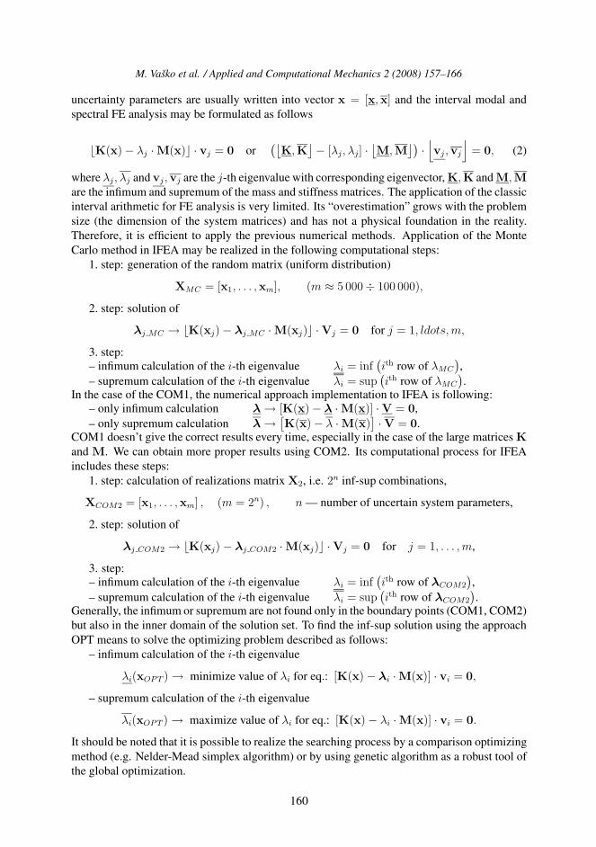
uncertainty parameters are usually written into vector x = [x,x] and the interval modal and

spectral FE analysis may be formulated as follows

�K(x) − λj · M(x)� · vj = 0 or(⌊

K,K⌋

− [λj, λj] ·⌊

M,M⌋)

·⌊

vj ,vj

⌋

= 0, (2)

where λj , λj and vj ,vj are the j-th eigenvalue with corresponding eigenvector, K,K and M,M

are the infimum and supremum of the mass and stiffness matrices. The application of the classic

interval arithmetic for FE analysis is very limited. Its “overestimation” grows with the problem

size (the dimension of the system matrices) and has not a physical foundation in the reality.

Therefore, it is efficient to apply the previous numerical methods. Application of the Monte

Carlo method in IFEA may be realized in the following computational steps:

1. step: generation of the random matrix (uniform distribution)

XMC = [x1, . . . ,xm], (m ≈ 5 000 ÷ 100 000),

2. step: solution of

λj MC → �K(xj) − λj MC · M(xj)� · Vj = 0 for j = 1, ldots, m,

3. step:

– infimum calculation of the i-th eigenvalue λi = inf(

ith row of λMC

)

,

– supremum calculation of the i-th eigenvalue λi = sup(

ith row of λMC

)

.In the case of the COM1, the numerical approach implementation to IFEA is following:

– only infimum calculation λ → [K(x) − λ · M(x)] · V = 0,

– only supremum calculation λ →[

K(x) − λ · M(x)]

· V = 0.COM1 doesn’t give the correct results every time, especially in the case of the large matrices K

and M. We can obtain more proper results using COM2. Its computational process for IFEA

includes these steps:

1. step: calculation of realizations matrix X2, i.e. 2n inf-sup combinations,

XCOM2 = [x1, . . . ,xm] , (m = 2n) , n — number of uncertain system parameters,

2. step: solution of

λj COM2 → �K(xj) − λj COM2 · M(xj)� · Vj = 0 for j = 1, . . . , m,

3. step:

– infimum calculation of the i-th eigenvalue λi = inf(

ith row of λCOM2

)

,

– supremum calculation of the i-th eigenvalue λi = sup(

ith row of λCOM2

)

.Generally, the infimum or supremum are not found only in the boundary points (COM1, COM2)

but also in the inner domain of the solution set. To find the inf-sup solution using the approach

OPT means to solve the optimizing problem described as follows:

– infimum calculation of the i-th eigenvalue

λi(xOPT ) → minimize value of λi for eq.: [K(x) − λi ·M(x)] · vi = 0,

– supremum calculation of the i-th eigenvalue

λi(xOPT ) → maximize value of λi for eq.: [K(x) − λi · M(x)] · vi = 0.

It should be noted that it is possible to realize the searching process by a comparison optimizing

method (e.g. Nelder-Mead simplex algorithm) or by using genetic algorithm as a robust tool of

the global optimization.

160

M. Vasko et al. / Applied and Computational Mechanics 2 (2008) 157–166

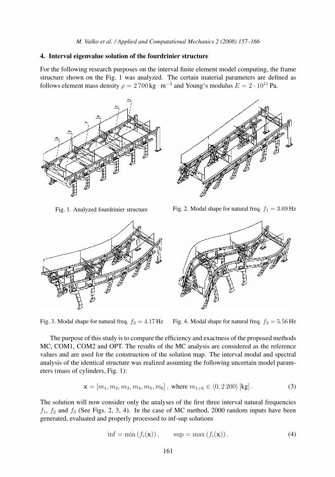
4. Interval eigenvalue solution of the fourdrinier structure

For the following research purposes on the interval finite element model computing, the frame

structure shown on the Fig. 1 was analyzed. The certain material parameters are defined as

follows element mass density ρ = 2 700 kg · m−3 and Young‘s modulus E = 2 · 1011 Pa.

Fig. 1. Analyzed fourdrinier structure Fig. 2. Modal shape for natural freq. f1 = 3.69 Hz

Fig. 3. Modal shape for natural freq. f2 = 4.17 Hz Fig. 4. Modal shape for natural freq. f3 = 5.56 Hz

The purpose of this study is to compare the efficiency and exactness of the proposed methods

MC, COM1, COM2 and OPT. The results of the MC analysis are considered as the reference

values and are used for the construction of the solution map. The interval modal and spectral

analysis of the identical structure was realized assuming the following uncertain model param-

eters (mass of cylinders, Fig. 1):

x = [m1, m2, m3, m4, m5, m6] , where m1÷6 ∈ 〈0, 2 200〉 [kg] . (3)

The solution will now consider only the analyses of the first three interval natural frequencies

f1, f2 and f3 (See Figs. 2, 3, 4). In the case of MC method, 2000 random inputs have been

generated, evaluated and properly processed to inf-sup solutions

inf = min (fi(x)) , sup = max (fi(x)) . (4)

161

M. Vasko et al. / Applied and Computational Mechanics 2 (2008) 157–166

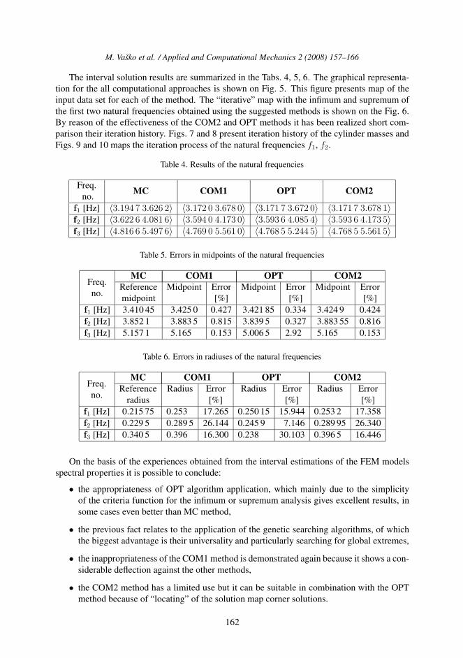
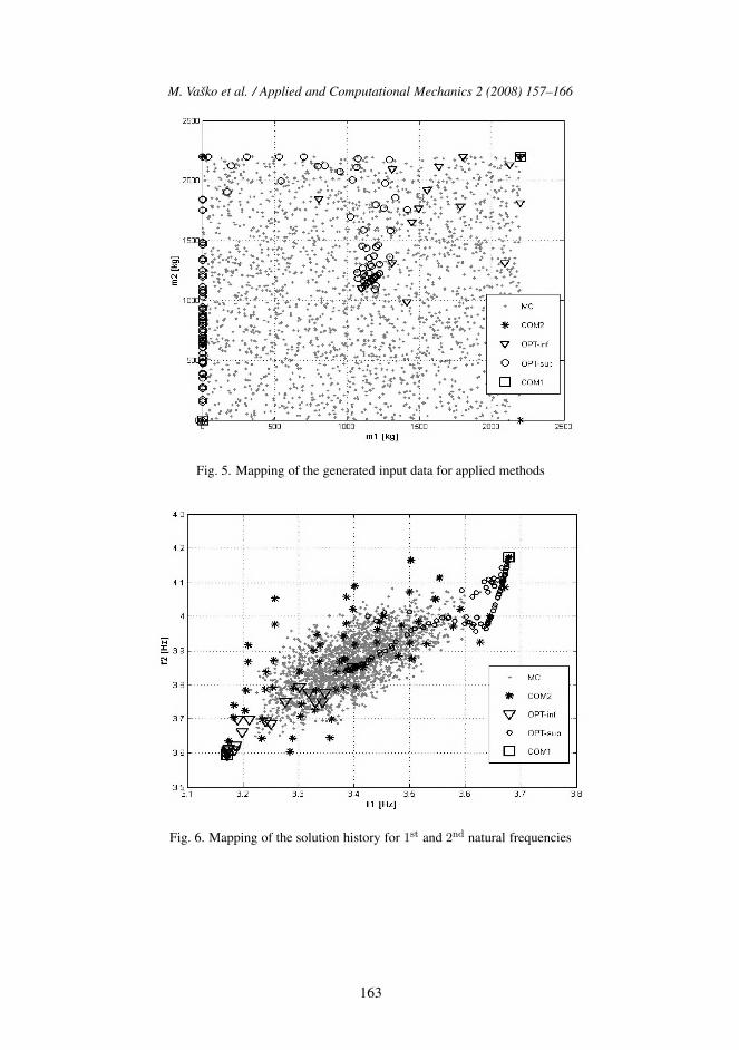
The interval solution results are summarized in the Tabs. 4, 5, 6. The graphical representa-

tion for the all computational approaches is shown on Fig. 5. This figure presents map of the

input data set for each of the method. The “iterative” map with the infimum and supremum of

the first two natural frequencies obtained using the suggested methods is shown on the Fig. 6.

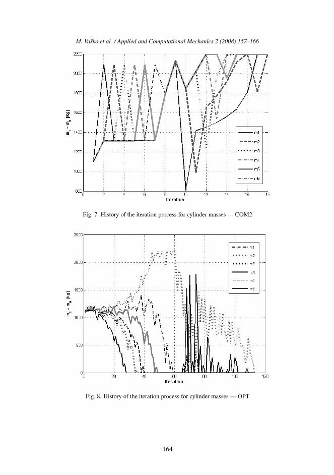
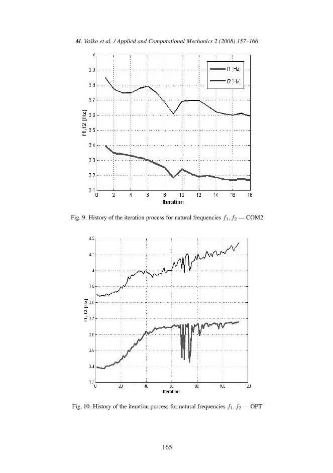
By reason of the effectiveness of the COM2 and OPT methods it has been realized short com-

parison their iteration history. Figs. 7 and 8 present iteration history of the cylinder masses and

Figs. 9 and 10 maps the iteration process of the natural frequencies f1, f2.

Table 4. Results of the natural frequencies

Freq.

no.MC COM1 OPT COM2

f1 [Hz] 〈3.194 7 3.626 2〉 〈3.172 0 3.678 0〉 〈3.171 7 3.672 0〉 〈3.171 7 3.678 1〉f2 [Hz] 〈3.622 6 4.081 6〉 〈3.594 0 4.173 0〉 〈3.593 6 4.085 4〉 〈3.593 6 4.173 5〉f3 [Hz] 〈4.816 6 5.497 6〉 〈4.769 0 5.561 0〉 〈4.768 5 5.244 5〉 〈4.768 5 5.561 5〉

Table 5. Errors in midpoints of the natural frequencies

Freq.MC COM1 OPT COM2

no.Reference Midpoint Error Midpoint Error Midpoint Error

midpoint [%] [%] [%]

f1 [Hz] 3.410 45 3.425 0 0.427 3.421 85 0.334 3.424 9 0.424

f2 [Hz] 3.852 1 3.883 5 0.815 3.839 5 0.327 3.883 55 0.816

f3 [Hz] 5.157 1 5.165 0.153 5.006 5 2.92 5.165 0.153

Table 6. Errors in radiuses of the natural frequencies

Freq.MC COM1 OPT COM2

no.Reference Radius Error Radius Error Radius Error

radius [%] [%] [%]

f1 [Hz] 0.215 75 0.253 17.265 0.250 15 15.944 0.253 2 17.358

f2 [Hz] 0.229 5 0.289 5 26.144 0.245 9 7.146 0.289 95 26.340

f3 [Hz] 0.340 5 0.396 16.300 0.238 30.103 0.396 5 16.446

On the basis of the experiences obtained from the interval estimations of the FEM models

spectral properties it is possible to conclude:

• the appropriateness of OPT algorithm application, which mainly due to the simplicity

of the criteria function for the infimum or supremum analysis gives excellent results, in

some cases even better than MC method,

• the previous fact relates to the application of the genetic searching algorithms, of which

the biggest advantage is their universality and particularly searching for global extremes,

• the inappropriateness of the COM1 method is demonstrated again because it shows a con-

siderable deflection against the other methods,

• the COM2 method has a limited use but it can be suitable in combination with the OPT

method because of “locating” of the solution map corner solutions.

162

M. Vasko et al. / Applied and Computational Mechanics 2 (2008) 157–166

Fig. 5. Mapping of the generated input data for applied methods

Fig. 6. Mapping of the solution history for 1st and 2

nd natural frequencies

163

M. Vasko et al. / Applied and Computational Mechanics 2 (2008) 157–166

Fig. 7. History of the iteration process for cylinder masses — COM2

Fig. 8. History of the iteration process for cylinder masses — OPT

164

M. Vasko et al. / Applied and Computational Mechanics 2 (2008) 157–166

Fig. 9. History of the iteration process for natural frequencies f1, f2 — COM2

Fig. 10. History of the iteration process for natural frequencies f1, f2 — OPT

165

M. Vasko et al. / Applied and Computational Mechanics 2 (2008) 157–166

5. Conclusion

The paper discusses the possibility of the interval arithmetic application in a modal and spectral

FE analysis. The interval arithmetic provides a new possibility of the quality and reliability

appraisal of analyzed objects. Due to this numerical approach, we can analyze mechanical,

technological, service and economic properties of the investigated structures more authentically.

In our paper we have investigated possibilities of the modal and spectral solution of a four-

drinier structure with an interval weight of the cylinders (according to condensed water). The

centre of our interest has been mainly to compare the suggested numerical algorithms and their

efficiency evaluation.

Acknowledgements

This work has been supported by VEGA grant No. 1/3168/06 and VEGA grant No. 1/4099/07.

References

[1] V. Dekys, A. Sapietova, R. Kocur, On the reliability estimation of the conveyer mechanism using

the Monte Carlo method. Proc. COSIM2006, Krynica — Zdroj, august 2006, pp. 67–74.

[2] Z. Kulpa, A. Pownuk, I. Skalina, Analysis of linear mechanical structures with uncertainties by

means of interval methods, Computer Assisted Mechanics and Engineering Sciences, 1998, Vol. 5,

Poland, pp. 443–477.

[3] R. E. Moore, Interval Analysis. Prentice Hall, Englewood Cliffs, New Jersey, 1966.

[4] S. Segla, Dynamic and quasistatic analysis of the elevating work platform, Journal Mechanisms

and Manipulators, Vol. 6, Nr. 1, 2007.

[5] A. Neumaier, Interval Methods for Systems of Equations. Cambridge University Press, Cam-

bridge, 1990.

[6] P. Forssen, Interval methods I.

http://www.tdb.uu.se/kurs/optim-mn1/ht01/lectures/lec14 2.pdf

[7] S. M. Rump, Intlab. http://www.ti3.tu-harburg.de/∼rump/intlab/

[8] I. Elishakoff, D. Duan, Application of Mathematical Theory of Interval Analysis to Uncertain

Vibrations, Proc. of NOISE-CON’94, Ft. Lauderdale, Florida, pp. 519–524, 1994.

[9] S. H. Chen, X. W. Yang, Interval finite element method for beam structures, Finite Elem. Anal.

Des., 34, 2000, pp. 75–88.

[10] H. Zhang, R. L. Muhanna, Finite element analysis for structures with interval parameters, Proc.

9th ASCE Joint Sp. Conf. on Probab. Mech. and Struct. Reliability, Albuquerque, New Mexico,

USA, 2004.

[11] H. Zhang, Nondeterministic Linear Static Finite Element Analysis: An Interval Approach, School

of Civil and Environmental Engineering, Georgia Institute of Technology, December 2005.

166