1

GP competition011212 25/01/2013 13:39

Competition, prices, and quality in the market for GP consultations

Hugh Gravelle* Anthony Scott** Peter Sivey** Jongsay Yong**

[WORK IN PROGRESS – PLEASE DO NOT CITE] Abstract General Practitioners (GPs) in Australia are free to set prices for consultations. Under the national tax funded Medicare insurance scheme patients pay the difference between the price set by the GP and a fixed reimbursement. GPs can ‘bulk bill’ the patient when the patient makes no out of pocket payment. We construct a Vickrey-Salop model of GP third degree price and quality discrimination with bulk billing. We test its predictions using a dataset with individual GP-level data on prices, the proportion of patients who are bulk billed, average consultation length, and characteristics of the GPs, their practices and patients. A key variable is the distance between a GP practice and its nearby competitors which allows us to use area fixed effects to account for endogeneity of GP location decisions. We find that within areas, GPs with more distant competitors charge higher average prices, mainly by reducing the proportion of patients who are bulk billed.

JEL: I11, I13, L1 Keywords: Competition. Prices. Quality of care. Primary care. Doctors.

Acknowledgements.

The research was supported by funding from Australian Research Council Discovery grant DP110102863. MABEL is supported by a National Health and Medical Research Council Health Services Research Grant (454799) and the Commonwealth Department of Health and Ageing. We thank the doctors who gave their valuable time to participate in MABEL, and the other members of the MABEL team. The views expressed are those of the authors and not necessarily those of the funders.

* Centre for Health Economics, University of York. ** Melbourne Institute for Economic and Social Research, The University of Melbourne

2

1 Introduction

The market for healthcare is idiosyncratic in many ways. Features of this market include

concerns for equity, supplier induced demand, barriers to entry on the supply side and high

levels of government subsidy and regulation in most countries. Despite these idiosyncrasies,

traditional aspects of industrial organisation such as market structure and the degree of

competition can have effects on health care costs, quality of care and access to health care.

Some features of the Australian market for GP services make it a particularly interesting

context to test for the effects of market forces. Prices for consultations are unregulated, and

innovative GP-level data is available, making this a good market in which to examine the

effects of competition on prices and quality. Our study has lessons for policy in other health

care systems with unregulated prices for physicians. These include France where some GPs

can charge fees above the government rebate (The Commonwealth Fund 2011), and the US,

where the practice of charging fees above the price reimbursed by the insurer is known as

balance billing (Glazer and McGuire, 1993).

Patients in Australia pay a fee for each GP consultation. The fees that GPs charge are not

regulated and they are also free to price discriminate between patients. The national, tax

financed, Medicare insurance scheme provides a subsidy for the cost of a consultation (the

Medicare rebate). The patient pays the excess of the GP fee over the Medicare rebate and

these out of pocket co-payments by patients cannot be covered by insurance. Simple intuition

and theoretical models (eg Cournot competition) would suggest that the number of local

competitors GPs face (GP density) may affect their incentives to charge fees above the

medicare rebate. The aim of this paper is to model and estimate the effect of GP density on

prices and quality in the market for GP consultations.

The majority of studies in the health economics literature examine the effect of competition

in hospital or insurance markets, with few studies on the effects of competition in the market

for physician services (Gaynor and Town, 2011). The literature on the influence of

competition on prices charged and a range of other physician behaviours has been reviewed

by Dranove and Satterthwaite (2000) and more recently by Gaynor and Town (2011). Studies

on competition and prices for physicians have often been conducted in the context of

supplier-induced demand and have suffered from identification problems due to the use of

3

area-level measures of competition. Small area measures can be correlated with

unobservable characteristics of areas that are also associated with the location choice of

physicians. Of the more recent studies, Schneider et al (2008) find that physician market

concentration in California, measured by the Herfindahl Hirschman Index (HHI) is associated

with higher prices. Bradford and Martin (2000) find that higher physician density is

associated with less profit sharing amongst physicians in group practices and lower prices.

Johar (2012) uses detailed patient-level data to look at the relationship between prices and

patient income in Australia. She also finds an interaction with GP density in this relationship,

GP density reduces the relationship between rich patients and higher prices.

Studies have also measured the degree of competition using structural models. One strand

uses estimates of physician cost functions and observed prices to estimate the degree of

competition in the market (Gunning and Sickles, 2012; Bresnahan, 1989). Schaumans and

Verboven (2008) have adapted Bresnahan and Reiss’ (1991) entry model to find the effect of

geographic entry restrictions on the number of pharmacies physicians in Belgium.

We add to this literature in several ways. First, we develop a formal model of GP third

degree price and quality discrimination under bulk billing with free entry into GP markets.

We use it to generate predictions about the effects of competition as a guide to our empirical

analysis. This builds on previous theoretical models. Glazer and McGuire (1993) use a

Hotelling model to examine how prices, bulk billing and quality vary with patient location.

Brekke et al (2010) have a Vickrey-Salop circular city model with an exogenous number of

doctors and all patients facing the same price and quality. There is no patient insurance and

so no possibility of bulk billing. They show that the effects of an increase in the number of

doctors on price and quality depend on assumptions about patient utility and doctor cost

functions. Gravelle (2000) also studies price and quality in a Vickrey-Salop model and

allows for entry by doctors but does not consider bulk billing or for prices and quality to vary

across patient types.

The second way we add to the literature is the method we use for identification. Previous

literature has relied on area level GP density measures and so is potentially vulnerable to

endogeneity bias if unobserved factors that influence entry and exit into areas are also

correlated with prices and qualities. We use a GP-level measure of GP density (distance to

nearby other GP practices) that allows us to use area fixed effects to control for all area-level

4

variables that are unobserved and may influence prices, including the characteristics of areas

that influence exit and entry into those areas. Identification therefore relies on within-area

variation in distance to other GPs. Our use of distance to measure competitive pressure

follows a strand in the literature which emphasizes distance to nearby competitors as a

determinant of prices (Alderighi and Piga 2012, Thomadsen 2005). Distance between firms

has also been found to be an important determinant of prices in studies of hospital

competition (Gaynor and Vogt 2003).

Third, most previous studies of the Australian market have relied on administrative data that

does not include detailed information on the influence of doctor or practice characteristics

(McRae 2009, Richardson et al 2006, Savage and Jones 2004). This is exacerbated by using

small area data which takes averages of GP and practice characteristics across areas and

therefore masks heterogeneity. Use of administrative data ignores the effects of sources of

heterogeneity that influence pricing decisions, in addition to the effect of competitive

pressure. For example, depending on the structure of a partnership, each GP in a practice

may: i) have full discretion to charge their own prices; ii) have discretion of whether to bulk-

bill some patients but not others; iii) may have to charge the price agreed by the owners of the

practice, or iv) may opt to bulk-bill all patients. These are decisions influenced by practice

characteristics and by patient characteristics, both of which may be correlated with the degree

and nature of competition. If these factors are not accounted for then the estimate of the effect

of GP density on prices may be biased.

Our theoretical model of the market for GP services generates testable hypotheses about the

relationship between price and quality variables, and a measure of competitive pressure: the

distance between GP practices. We find results consistent with the predictions from our

theoretical model. GPs whose rivals are further away charge higher average prices. This

result is robust to alternative estimation strategies, including area fixed-effects estimations.

Although distance to rivals tends to reduce quality the effects are not always statistically

significant. The main reason for higher average prices for GPs with less competition is that

they bulk bill a smaller proportion of their patients. We also find that these effects of

competition are stronger in areas of greater socio-economic advantage.

2 Institutional setting

5

General practitioners in Australia are paid by fee-for-service for consultations. They are free

to charge what the market will bear. Their patients are subsidised by Medicare, a national tax-

financed insurance scheme. Patients can claim back a fixed rebate from Medicare as set out in

the Medicare Benefits Schedule (Australian Government, 2008). Co-payments by patients

(the difference between the rebate and the price charged) cannot be covered by insurance.

GPs can choose to ‘bulk-bill’ a patient, so that the patient pays nothing to the GP who claims

the rebate direct from Medicare as full payment. Some GP practices choose to bulk-bill all

patients, whilst GPs in other practice bulk bill none or only a proportion of their patients.

There are some incentives for bulk billing, in the form of a higher medicare rebate, for certain

groups of patients, mainly children and the elderly.

There is no enrolment of patients or list system. Patients can choose to visit any GP practice

each time they consult. GPs are gatekeepers to specialist and hospital services, though

patients can access hospital services directly through emergency departments which can

substitute for GP services. There are no restrictions on geographical location of practice,

apart from doctors arriving from overseas who must first practice for a set period in under-

doctored areas. GPs in designated geographical areas of workforce shortage are eligible for a

range of payments to encourage them to locate to and remain in these areas.

There has been increasing concentration in the market for GP services. Between 2003 and

2008, although the number of GPs in Australia grew by 4.6% the number of GP practices fell

by 6.7% (Moretti et al 2010). Both state and federal government policy has encouraged the

formation of larger practices, with current policy funding the establishments of ‘GP

Superclinics’. Increasing concentration could also be explained by a trend for private

companies to own chains of large GP practices. Our study is partly motivated by predicting

the outcomes of these trends in terms of prices and quality.

3 A model of bulk billing, price and quality

3.1 Specification

We model GPs’ decisions and the market equilibrium by extending the Vickrey-Salop model

of monopolistically competitive firms (Vickrey, 1964; Salop, 1979) to include choice of

quality as well as prices and for the possibility that GPs bulk bill a proportion of their

patients.

6

The total price per consultation received by a GP is p + m where m is the price paid to the GP

by Medicare. Patients pay p per consultation. Patients demand at most one consultation per

period from their GP and the utility gain from a consultation at GP i is

ui = r pi + αqi tdi (1)

where pi is the price the patient pays at GP i, qi is the quality of the consultation (measured

say by its length), di is the distance to the GP, α [α0,α1] and t are taste parameters. We

assume that r is large enough to ensure that the market is covered: all patients demand a

consultation. All patients have the same marginal disutility of expenditure and the same

marginal disutility of distance t. They differ in their marginal valuation of quality (α).

There are H patients in total, distributed uniformly around the circular market of length L, so

that the density of patients at any point in the market is h = H/L. The probability distribution

and density functions of patient types, F(;θ) and f(;θ), are independent of location within

the market, so that at each point there are hf(;) patients of type . shifts the patient type

distribution. We assume that markets with higher have higher mean marginal valuations

of quality.

G GPs are equally spaced around the market so that the distance between GPs is = L/G.

GPs observe patient types and can charge different prices and provide different quality to

each type. The demand for GP i from type α patients depends on the price pi(α) she charges

them and the quality qi(α) she provides, as well as the prices and qualities of her immediately

neighbouring GPs:1

1 1

( ; )( ) ( ) [ ( ) ( )]

2i i i i i

hfD p p q q t

t

1 1

( ; )( ) ( ) [ ( ) ( )]

2 i i i i

hfp p q q t

t

1 1 1 1( ( ), ( ); ( ), ( ), ( ), ( ), , , , )i i i i i iD p q p q p q h (2)

where the first term is demand from patients between GP i and GP i + 1 and the second is

demand from patients between GP i and GP i 1.

1 See Gravelle (1999), Brekke et al (2010).

7

Although GPs can observe willingness to pay for quality for each patient we assume that

there are costs to them of exercising fine degrees of price and quality discrimination and that

they discriminate only between two groups of patients (third degree price discrimination).

The GP sets a threshold patient marginal valuation of quality ˆi and GP bulk bills (pi(α) = 0)

all patients with ˆi , and gives the same price (pi(α) = pi > 0) 2 to all patients with > ˆ

i .

All patients who are bulk billed get quality qi(α) = q0i and those who are not bulk billed get

quality qi(α) = q1i.

Demand from bulk billed patients of GP i is

0

ˆ

0 1 1 1 1(0, ; ( ), ( ), ( ), ( ), , , , )i

i i i i iD q p q p q h d

= 0

ˆ

0 0 0 0ˆ; , , ;

i

i i iD q d D q

(3)

so that the marginal effect of quality on demand from bulk billed patients is

0

0

ˆ

0 0 ˆ, ; ( ; ) 0i

iq i i

hD q f d

t

(4)

Demand from non-bulk billed patients is

1

1 1 1 1 1ˆ( , ; ( ), ( ), ( ), ( ), , , , )

ii i i i i iD p q p q p q h d

= 1

1 1 1 1ˆˆ, ; , , , ;

ii i i i iD p q d D p q

(5)

and

1

11 1 ˆˆ, , ; ( ; ) 0

ii

q i i i

hD p q f d

t

(6)

1

1 1 ˆˆ ˆ, , ; ( ; ) 1 ; 0

ii

p i i i

h hD p q f d F

t t

(7)

The average variable cost of serving patients who get quality q is ½δq2 and so GP i profit is

2 21 10 1 0 0 0 1 1 12 2

ˆ ˆ ˆ, , , ; , ; , , ;i i i i i i i i i i i i iq p q D q m q D p q p m q (8)

The GP chooses q0i, pi, q1i, and ˆi to maximise πi. First order conditions are

0 0 0 0

ˆ( , ; )iiq i i iq D q 21

0 0 02ˆ, ; 0

ii q i im q D q (9)

2 It can never be optimal to set p < 0 (ie pay the patient in order to get the Medicare rebate m) since increasing p to zero, with quality constant, has no effect on demand (since patients pay nothing in both cases) and therefore no effect on costs, and increases revenue.

8

211 1 1 1 12

ˆ ˆ, , ; , , ; 0i iip i i i i p i iD p q p m q D p q (10)

1 1 1 1

ˆ, , ;iiq i i i iq D p q

1

211 1 12

ˆ, , ; 0ii i q i i ip m q D p q (11)

2 21 1ˆ 0 1 0 12 2

ˆ ; 0i i i i ii m q p m q f (12)

where λ0, λ1 are Lagrange multipliers on the constraints on the threshold ( ˆi α0 0, α1 ˆ

i

0).

With identical GPs there is a symmetric Nash equilibrium in which GPs make the same

choice of threshold, qualities, and price to non-bulk billed patients. We can now drop the GP

specific subscript. At the equilibrium, demand for each GP for bulk billed and non-bulk billed

patients is

0

ˆ

0 1 ˆˆ ˆ, ; ( ; ) ;D q h f d h F

(13)

1

1 1 ˆˆ ˆ, , ; ( ; ) 1 ;D p q h f d h F

(14)

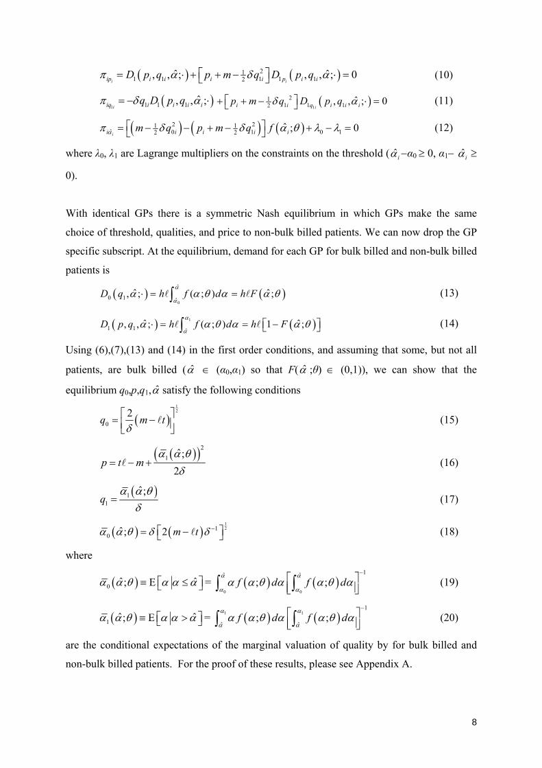
Using (6),(7),(13) and (14) in the first order conditions, and assuming that some, but not all

patients, are bulk billed (̂ (α0,α1) so that F(̂ ;θ) (0,1)), we can show that the

equilibrium q0,p,q1,̂ satisfy the following conditions

12

0

2q m t

(15)

2

1 ˆ;

2p t m

(16)

11

ˆ;q

(17)

121

0ˆ; 2 m t (18)

where

0 ˆ ˆ; E = 0 0

1ˆ ˆ; ;f d f d

(19)

1 ˆ ˆ; E = 1 11

ˆ ˆ; ;f d f d

(20)

are the conditional expectations of the marginal valuation of quality by for bulk billed and

non-bulk billed patients. For the proof of these results, please see Appendix A.

9

3.2 Model predictions

We do not observe prices and quality for individual patients but we do have data from each

GP in our sample (see section 4.1) which enables us to measure

a) the proportion of each GP’s patients who are bulk billed: Fb =F(̂ ; );

b) the price charged to patients who are not bulk billed: p;

c) the average price charged to all patients: ( 0) (1 )b bp F F p = (1 )bF p ;

d) the average quality of GP’s consultation (as measured by average consultation time

for all her patients): q = Fbq0 + (1Fb)q1;

We use the model to derive predictions about how these variables respond to an increase in

= L/G which we interpret as a decrease in competition in the market.

a) We use (18) and (19) to derive the effect of an increase in distance between GPs on the

proportion bulk billed F(̂ ; ). The expectation of the value of quality α for those who are

not bulk billed ( 0ˆ; ) is monotonically increasing in the threshold ̂ for ̂ (α0,α1).

Thus, using condition (18) for the last equality,

1

210 0ˆ; ˆ ˆ

sgn sgn sgn sgn sgn 2 0ˆ

Ft m t

(21)

and an increase in the distance between GPs reduces the proportion of patients bulk billed.

b) The effect of on the price to non-bulk billed patients is

1 11 1

ˆ ˆ; ; ˆ1 1ˆ ˆ

ˆp

t t

(22)

Since both 0ˆ and 1

ˆ are monotonically increasing in ̂ for ̂ (α0,α1) we can

sign the second term in (22) using (18):

0 01 1 ˆ ˆsgn sgn sgn sgn 0

ˆ ˆ

(23)

Thus the effect of an increase in the distance between GPs on the price charged to non-bulk

billed patients is ambiguous. For the intuition we can use the expression (10) for the

marginal profit from an increase in price. An increase in increases the number of non-bulk

billed patients that the GP has, since from (14) dD1/d = h(1F) h f̂ / >0 and

increases thus the gain from a price increase if no patients move to another GP. But, from

10

(7), the increase in increases the average responsiveness of patients to the price because the

reduction in ̂ that the average patient now values the GP less highly and is therefore more

likely to move to another GP.

c). Distance between GPs also has an ambiguous effect the average price charged to all

patients p = (1F)p. From (16)

2

11 1ˆˆ ˆ ˆ

ˆ ˆ1 ; ;ˆ

pt F t m f

(24)

The second term is positive since ˆ / < 0 but, since 1ˆ/ > 0, the first term in the first

square bracket is negative, and effect on the average price is ambiguous.

d) It is immediate from (15) that an increase in reduces the quality q0 supplied to bulk

billed patients and, since from (23) 1 / < 0, q1 is also reduced, the average quality for all

patients q is also reduced.

The top part of Table 1 shows the comparative static responses of these five variables to

changes in distance between GPs and other model parameters for solutions where no patient

is bulk billed (Fb = 0), some are bulk billed (Fb (0,1)) and all patients are bulk billed Fb = 1.

3.3 Endogeneity of competition measure

We test for the effects of reduced competitive pressure (increased ) by estimating cross-

section regression models of the prices and qualities chosen by GPs in different markets with

differing amounts of competitive pressure. However, in the absence of restrictions on entry

the number of GPs in a market and hence the distance between GPs ( ) is endogenous which

raises the possibility that simple cross-section model will produce biased estimates of the

effect of .

With free entry into different markets, in equilibrium all markets will yield the same profit.

GP profit at the Nash equilibrium with a given number of GPs is * ( ; , , , , )t m h . Denote

GP fixed cost of operating in the market by K (which can be taken to be a financial cost

minus the monetary equivalent of any utility from the amenities in the market).

11

The equilibrium number of GPs and hence the distance between GPs is determined by the

condition that GPs break even:

* ( ; , , , , ) 0t m h K (25)

so that in equilibrium the distance between GPs is

( , , , , , )t m h K (26)

Using the implicit function rule on (25) the effects of , t etc on the equilibrium are /

= * */ etc and these are reported in the bottom part of Table 1.3

Endogeneity of will lead to biased estimates if the estimated model omits variables which

determine prices or qualities and are correlated with . For example, the true model for the

bulk billing proportion is Fb = ˆ( ( , , , ); )F t m = ( ( , , , , ), , , , )bF m h K t m . If the

regression fails to include variables like t which affect both Fb and negatively, the

estimated effect of will be positively biased. Omission of measures of variables like θ

which only affect Fb and are not correlated with will not bias the estimated effect of ,

though it will lead to a loss of efficiency. Finally, variables like K which only affect Fb

though their effect on should be omitted from the regression, though they could act as

instruments for . We discuss how we implement the estimation of the regression models in

more detail in section 4.2 after describing the data.

4 Empirical Methods

4.1 Data

We use data from the first wave of the MABEL survey, a prospective cohort/panel study of

workforce participation, labour supply and its determinants among Australian doctors. The

sampling frame is the Australian Medical Publishing Company’s (AMPCo) Medical

Directory, a national database of all Australian doctors, managed by the Australian Medical

3 When the some but not all patients are bulk billed, use the fact that the profit per patient is the same for bulk

billed and non-bulk billed patients, so that 2102m q = 21

12p m q and substitute in the optimal values of p,

q0, q1 from (16), (15), (17) to get * 2h t . When no patient is bulk billed, π* = 2112h p m q , and

substitution for the optimal p and q1 also gives * 2h t . When all patients are bulk billed profit is

2102h m q and optimal q0 is determined by (40) and so π* is now function of m and δ as well as h, t and .

12

Association (AMA). Data was collected from June to December 2008. The questionnaire

covered topics such as job satisfaction and attitudes to work; characteristics of work setting

(public/private hospital, private practice); workload (hours worked, on-call); finances

(income, income sources); geographic location; demographics; and family circumstances

(partner and children).

The number of GPs responding in the first wave was 3906 (including 226 GP registrars

(trainees)), a response rate of 19.36%. The respondents were nationally representative with

respect to age, gender, geographic location and hours worked (Joyce et al. 2010). We restrict

the study sample to GPs located in the major conurbations in Australia. The areas outside

these conurbations are sparsely populated and GPs in them face different financial incentives

and regulations to those in our study sample. After excluding rural GPs, GP registrars, and

those with incomplete data we had a study sample of 1925 GPs.

Prices

The survey asks two questions about consultation fees. The first is “Approximately what

percentage of patients do you bulk bill/charge no co-payment?” We use this measure the

proportion of patients who are bulk billed (Fb). Patients who are bulk-billed are charged no

copayment and the GP is paid the Medicare rebate (m).

The second question is“What is your current fee for a standard (level B) consultation?

(Include Medicare rebate and patient co-payment. Please write amount in dollars; write 0 if

you bulk bill 100% of your patients)” which we use as a measure of the price charged to

patients who are not bulk billed. Different types of consultation (defined in terms of

complexity and length) have different Medicare rebates and may have different copayments

set by GPs.4 However, in 2008 level B consultations represented 88.4% of all GP

consultations and we believe the answer to this question will be a good measure of a GP’s

4 The Medicare Benefits Schedule has four categories of consultation (Australian Government, 2008). Level A are simple consultations with limited examination, for example a consultation for a tetanus immunisation. Level B are more complex than Level A and include history taking, advice giving, ordering tests, formulation and implementation of a management plan. Level C are more complex than level B and must last at least 20 minutes. Level D consultations are yet more complex and must last at least 40 minutes. In 2008, Level B consultations were the most common (88.4% of all GP attendances), followed by Level C (10.5%), with the others Levels A and D just over 1%.

13

price setting behaviour for non-bulk billed patients relative to other GPs facing different

market conditions.

Quality

The GPs are asked “How long does an average consultation last? (Please write number of

minutes)”. Since consultation length is positively correlated with measures of the quality of

care including preventative care, lower levels of prescribing and some elements of patient

satisfaction (Wilson and Childs 2002), we use this variable as a measure of the average

quality of consultations ( q ).

Competition measure

There is a large literature on measuring competition in healthcare markets (Gaynor and

Town, 2011). Studies on markets for hospital care often calculate Herfindahl-Herschmann

indices (HHIs) based on market share information. Recent studies have used the approach of

Kessler and McClellen (2000) and Gowrisankaran and Town (2003), to avoid the

endogeneity problem that market share depends on a prices and qualities, by calculating the

HHI from regression estimates of demand which include distance but not price or quality.

Studies in physician markets generally have not been able to take this approach (with the

exception of Schneider et al, 2008) because of the absence of data on patients’ residential

location. Instead, most physician market studies have used a measure of physician density

(Bradford and Martin 2000, Richardson et al 2006) in an area. This has the disadvantage that

it is endogenous and that all providers in an area are assumed to face the same competitive

pressure.

We construct an individual-level variable measuring competition, the distance between a

GP’s practice and her rival practices. This approach follows directly from the model in

section 3 where we use distance between GPs as a measure of competition. Several papers

in the hospital competition literature have also used competition measures which are purely

geographically defined (Propper et al, 2008). Recent literature in Industrial Organisation has

emphasised the importance of distance to competitors, rather than market share measures (eg

the HHI) on pricing decisions (Thomadsen 2005, Alderighi and Piga 2012). Drawing on

Bresnahan and Reiss (1991), who show in a variety of industries that only the first three

14

additional competitors in a given market have a large effect on prices, we use specifications

of using the distance to the 3rd and 5th nearest other GP practice.

We construct the competition measures using data from the Australian Medical Publishing

Company (AMPCo) which covers the whole population of Australian GPs, not only those

who responded to the MABEL survey. We calculated the road distances between GP

practices’ street addresses. For each MABEL respondent we calculated the distance to the

nearest, third nearest, and fifth nearest other GP practice in the AMPCo data (whether or not

they were MABEL respondents).

GP and GP practice covariates

We control for a number of individual GP and GP practice characteristics to allow for

differences in costs or preferences across practices which may influence pricing decisions.

First, we control for GP gender and whether they have a spouse or dependent children.

Second, we control for professional characteristics of the GP: whether they went to an

Australian medical school, their level of experience (in ten year bands), and whether they are

a partner or associate in a practice. Being a partner or associate indicates a direct financial

(ownership) relationship with the practice which may give incentives to charge higher prices.

Partner or associate status also indicates seniority of the GP within the practice. Third, we

control for the characteristics of the practice itself. These include practice size (number of

GPs) and whether the practice is taxed as a company or not. Practice size may influence

pricing decisions either via economies of scale or via its incentive effects (Gaynor and Pauly,

1990). Being a company may reflect the extent of ‘for-profit’ objectives of the GP’s practice.

Local area characteristics

We use data on area characteristics to capture factors which may affect demand and cost

conditions for GPs. There are two definitions of areas we use in the analysis, Statistical local

areas (SLAs) and postcode areas. The 1925 GPs in the estimation sample are located in 412

Statistical Local Areas (SLAs) with an average population of 33,023. The postcode areas are

slightly smaller, there are 628 postcode areas. We attribute Census data on the postcode age

distribution, ethnicity, self reported disability and socio-economic status through the Socio-

Economic Index for Areas (SEIFA). The SEIFA Index of Relative Socio-Economic

Advantage and Disadvantage is constructed by the Australian Bureau of Statistics from 22

variables measuring education, income, occupational structure, employment status, and

15

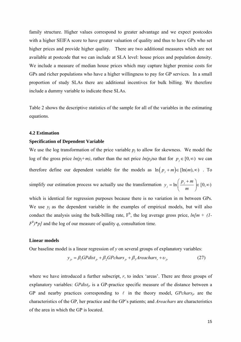
family structure. Higher values correspond to greater advantage and we expect postcodes

with a higher SEIFA score to have greater valuation of quality and thus to have GPs who set

higher prices and provide higher quality. There are two additional measures which are not

available at postcode that we can include at SLA level: house prices and population density.

We include a measure of median house prices which may capture higher premise costs for

GPs and richer populations who have a higher willingness to pay for GP services. In a small

proportion of study SLAs there are additional incentives for bulk billing. We therefore

include a dummy variable to indicate these SLAs.

Table 2 shows the descriptive statistics of the sample for all of the variables in the estimating

equations.

4.2 Estimation

Specification of Dependent Variable

We use the log transformation of the price variable pj to allow for skewness. We model the

log of the gross price ln(pj+m), rather than the net price ln(pj)so that for [0, )jp we can

therefore define our dependent variable for the models as ln [ln( ), )jp m m . To

simplify our estimation process we actually use the transformation ln [0, )jj

p my

m

which is identical for regression purposes because there is no variation in m between GPs.

We use yj as the dependent variable in the examples of empirical models, but will also

conduct the analysis using the bulk-billing rate, Fb, the log average gross price, ln[m + (1-

Fb)*p] and the log of our measure of quality q, consultation time.

Linear models

Our baseline model is a linear regression of y on several groups of explanatory variables:

1 2 3jr jr r jrjry GPdist GPchars Areachars (27)

where we have introduced a further subscript, r, to index ‘areas’. There are three groups of

explanatory variables: GPdistjr is a GP-practice specific measure of the distance between a

GP and nearby practices corresponding to in the theory model, GPcharsjr are the

characteristics of the GP, her practice and the GP’s patients; and Areachars are characteristics

of the area in which the GP is located.

16

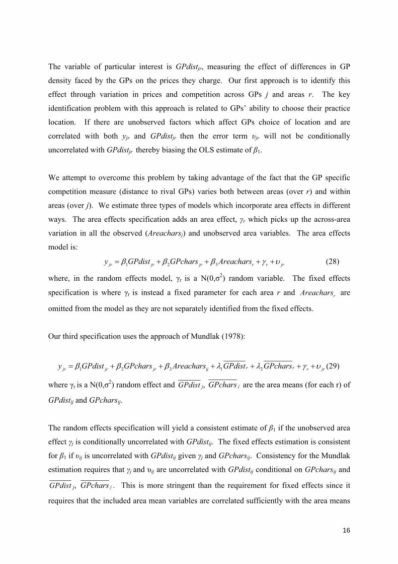
The variable of particular interest is GPdistjr, measuring the effect of differences in GP

density faced by the GPs on the prices they charge. Our first approach is to identify this

effect through variation in prices and competition across GPs j and areas r. The key

identification problem with this approach is related to GPs’ ability to choose their practice

location. If there are unobserved factors which affect GPs choice of location and are

correlated with both yjr and GPdistjr then the error term υjr will not be conditionally

uncorrelated with GPdistjr thereby biasing the OLS estimate of β1.

We attempt to overcome this problem by taking advantage of the fact that the GP specific

competition measure (distance to rival GPs) varies both between areas (over r) and within

areas (over j). We estimate three types of models which incorporate area effects in different

ways. The area effects specification adds an area effect, γr which picks up the across-area

variation in all the observed (Areacharsj) and unobserved area variables. The area effects

model is:

1 2 3jr jr r jrjr ry GPdist GPchars Areachars (28)

where, in the random effects model, γr is a N(0,σ2) random variable. The fixed effects

specification is where γr is instead a fixed parameter for each area r and rAreachars are

omitted from the model as they are not separately identified from the fixed effects.

Our third specification uses the approach of Mundlak (1978):

1 2 3 1 2r rjr jr jr ij r jry GPdist GPchars Areachars GPdist GPchars (29)

where γr is a N(0,σ2) random effect and GPdist j, jGPchars are the area means (for each r) of

GPdistij and GPcharsij.

The random effects specification will yield a consistent estimate of β1 if the unobserved area

effect γj is conditionally uncorrelated with GPdistij. The fixed effects estimation is consistent

for β1 if υij is uncorrelated with GPdistij given γj and GPcharsij. Consistency for the Mundlak

estimation requires that γj and υij are uncorrelated with GPdistij conditional on GPcharsij and

GPdist j, jGPchars . This is more stringent than the requirement for fixed effects since it

requires that the included area mean variables are correlated sufficiently with the area means

17

of omitted variables to absorb their entire effects. The fixed effect estimator ensures that the

across area effects of omitted variables are picked up by the area effect γj.

Using the Mundlak or fixed effects specification means that β1 is identified only from within-

area variation and we need sufficient variation in both yjr and GPdistjr within areas to

successfully identify β1. The advantage of including area effects in the estimation is that it

controls for characteristics of areas that would otherwise be unobserved but which may

influence prices, including demand side influences such as socio-economic status, age-gender

composition of the population, and supply-side influences, such as the availability of other

health services that may be substitutes for GP care (eg the number of pharmacies and

emergency departments).

In section 4.1 we discussed the two alternative area definitions we use for attributing area

characteristics (such as ethnicity and socio-economic status). For the Mundlak and area fixed

effects models ((28) and (29)) we use the slightly larger SLA definition of areas to estimate

the models, as these provide more within-area variation (an average of 4.7 GPs per SLA in

the sample, rather than 3.1 GPs per postcode). We include a robustness check using the

smaller postcode areas for these models.

Tobit model of GP prices

In addition to the linear models, we exploit the availability of data on the price to non bulk

billed patients pj and the proportion of patients bulk-billed, Fb in a tobit model.

We derive our estimation approach from the patient-level model where i and j index

respectively patient i jS , where Sj patients are treated by GPj and GP j=1,...,N. Let pij

denote the fee charged by GP j to patient i.

Let . and . denote respectively the normal cdf and pdf. The log-likelihood of the tobit

model is:

1 1

ln ln l 1n 1 lnjSN

ij j jij ij

j i

p X XL d d

(30)

where dij=1 if pij>0 (if the price is non-censored), and dij=0 otherwise.

18

We adapt the standard tobit framework at the patient-level given in (30) to allow data at the

GP level which includes the proportion of patients bulk-billed (for whom pij* censored at

zero) and the price for non bulk-billed patients (for whom pij*= pj is not censored). To apply

the tobit model we assume all patients are either charged the same price by a GP, or are bulk-

billed by that GP (pij=0). We then split each GP observation into two observations: one for

the patients who are bulk-billed, and one for non bulk-billed patients. This approach can be

derived by rearranging the likelihood function in (30) to take the form:

1

ln ln ln 1lnN

j j jij j ijij i

p X XL d S d

(31)

Let j be the proportion of non-bulkbilled patients seen by GP j, /j i ij jd S . Now

we can write the likelihood:

1

lnln ln 1 ln 1N

j j jj j

jj

p X XL S

(32)

In our implementation of the model we set Sj=S for all GP’s so that it is just a scalar

multiplying the likelihood and can be removed. In other words, we do not weight each GP’s

observation by the number of patients treated by that GP, we just use the proportion of

patients bulk-billed to weight. We can use data on πj, pj and Xj for each GP to estimate the

model. Following from our approach with linear models we can replace pj with

ln jj

p my

m

. The proportion of bulk-billed patients πj, is the quantity Fb in the theory

model.

The following three quantities will be of interest in our results:

1) The probability that a patient is bulk-billed by GP j:

Pr( 0) 1 /j jy X (33)

2) The average log price for non-bulk-billed patients

[ | ( )] /0j j j jXE y y X (34)

where ( / ) ( / ) / ( / )j j jX X X

3) The average log price for all patients

/ ) ( /[ ] Pr( 0)* [ | 0] ( )j j j j j jjE y y E y y X XX (35)

19

The vector of explanatory variables, X, will be specified as in the linear model in equation

(27). We also estimate a version of the tobit with the Mundlak area-average terms as in

equation (29).

5 Results

Linear Models

Table 3 presents detailed results for the regression models with the dependent variable log

average price from the four linear estimation methods. All models have standard errors

corrected to allow for clustering at area (SLA) level.5 The first row of coefficients (and

associated standard errors) are for our main competition measure GPdist, the log of the

distance to the third-nearest GP practice. There are statistically significant positive

coefficients for the distance to the third-nearest GP practices in all estimated models: the

further the distance to nearby competitors, the higher the average price charged by the GP.

The size of the effect is consistent across the alternative models, including the Mundlak and

fixed effects models, which control for the unobserved area-level characteristics.

Tobit models

Table 4 presents results from tobit models with the same dependent variable - log average

price. Two versions of the model are presented, first the standard tobit, then the tobit with

within-area Mundlak terms. The pattern of results are similar to the linear models but the

estimated marginal effects (in Table 5) are larger, 0.019 and 0.017 for the tobit models

compared to 0.017 and 0.015 for the equivalent linear models. This larger marginal effects

represents the fact that the tobit accounts for censoring in the GP pricing decision.

Alternative price and quality outcomes

Table 5 presents the estimates of the coefficient on GPdist from linear regression and tobit

models for the four other measures of GP pricing and quality decisions (the proportion bulk

billed Fb, log average price to those not bulk billed ln(p + m) the log average price over all

patients ln 1 bm F p , and average quality q ). The signs of the estimated coefficients

are in line with a key prediction of the theory model: greater distance to rival GPs is

associated with a lower bulk billing rate. Distance to rivals is also associated with a higher

5 The 1798 GPs are located in 1296 practices. We also allowed for clustering at practice level but this made little difference to the results.

20

price to non bulk billed patients and a higher average price, although the theory model was

ambiguous about these coefficients. Finally distance to rivals is associated with lower quality

(consultation time) although this is only marginally statistically significant in the area fixed

effects and Mundlak models, and not at all in the other models. The estimated coefficient for

the bulk billing rate is the most highly statistically significant across all models, suggesting

that the main effect of distance to nearby competitors on the average price m + (1 )bF p is

through the bulk billing rate Fb.

Interaction terms

Table 6 presents the same models as Table 5 with one additional coefficient – an interaction

term between GPdist and the socio-economic status of the local area. In the fixed effects and

Mundlak models the interaction with the index of local area advantage is statistically

significant in the models for price for non bulk billed patients, average price, and bulk billing.

In each case, the socio-economic advantage of the area strengthens the effects of distance to

local competitors on the price or quality outcome. As such, distance to local competitors has

a stronger positive effect on price and average price in advantaged areas, and a stronger

negative effect on bulk billing in more advantaged areas. The interaction term is not

significant in the quality model.

Other explanatory variables

Whether the GP graduated from an Australian medical school, and whether they are a partner

or associate in the practice, also predicts higher average price in all models. More

experienced GPs, and those in larger practices, appear to have higher average prices in

general, but this effect is not consistently statistically significant across the models. Family

and personal characteristics, and whether the practice is taxed as a company, does not appear

to influence quality standardised prices.

GPs in advantaged areas and areas with higher house prices are more likely to charge higher

prices, as are those in areas with a high proportion of 65 year olds. GPs in areas that have a

higher proportion of the population from south east Europe tend to charge lower average

prices.

21

6 Discussion

Our results broadly support the hypotheses generated by the model in section 3 (given in

Table 1). The baseline measure of GPdist ( ) as the log of distance to third-nearest GP

practice, is significantly negatively associated with the proportion of patients who are bulk

billed Fb and with the average price. Because the baseline dependent variable (log average

gross price) and the explanatory variable of interest are both in logs, we can interpret the

coefficient (in the linear models) or marginal effect (in the tobit models) as an elasticity. The

tobit model (with Mundlak adjustment) estimates an elasticity of 0.022, which is a small

effect of distance to competitors on prices charged. When we consider a 1 standard deviation

(1.5km) increase in the distance to the third nearest GP this predicts a $0.91 increase in the

average gross price and a 3.2 percentage point fall in the number of patients bulk-billed. As

we are using distance to measure competitive pressure, we might be interested in the

extremes of the distribution of competition. Shifting a GP from the lowest decile of the

distribution of distance to third nearest GP (0.28km) to the top decile (3.0km) is associated

with $2.18 increase in the average price and a 7.7 percentage point reduction in the

proportion of patients who are bulk billed (ie face zero copayment).

We also find that the interaction between local area socio-economic status and distance to

local competitors is statistically significant. In areas with higher socio-status an increase in

the distance to rival GPs is associated with a larger increase in the average price and a larger

reduction in the proportion of patients who are bulk billed. This is in line with the results of

Johar (2012) who uses patient-level data and finds an interaction between patient income and

the effect of GP density. While Johar uses area-level GP density, we find the same result

with our GP-level measure of distance to other GP practices.

We interpret the results from the fixed effect models as evidence of a causal effect of distance

to nearby competitors on GP pricing decisions. We think it reasonable to assume that omitted

variables correlated with the competition measure and pricing decisions operate mainly at the

area (SLA) level. This requires either that factors affecting GP location operate across SLAs

and not within them or that factors shifting demand or cost functions and thereby affecting

price are fairly homogenous within SLAs and vary mainly across them. The fact that we

find similar sized effects on average price in the models with and without area effects

22

suggests that our area-level variables capture most area-level factors that are correlated with

pricing decisions and our measures of competition.

Our results align with recent literature emphasising the importance of distance between

competitors in measuring competitive pressure (Thomadsen 2005, Alderighi and Piga 2012).

They also add support to the research which shows distance to competitors affects prices in

the healthcare market (Gaynor and Town 2003). The results are also broadly in agreement

with previous studies of the Australian market using area-level data which shows a higher GP

density increases the bulk-billing rate (Richardson et al 2006, Savage and Jones 2004).

Our results suggest that the trends to increasing concentration in markets for physician

services in the US and Australia where physicians can set prices as well as quality may lead

to higher prices and lower quality. The trend in Australia has arisen, not because of fewer

physicians, but because of an increase in the number of physicians per practice so that the

number of practices per head of population has fallen. This trend is in part due to

government policy to encourage larger practices in the belief that there are benefits by way of

cost reductions associated with economies of scale in larger practices. With data from a

single cross-section we cannot tell if the overall welfare effects of larger firms are positive or

negative but it does seem that patients of GPs facing less competition will, at any point in

time, face higher average prices.

23

References Alderighi, M. and Piga, C. 2012. Localized competition, heterogeneous firms, and vertical relations. The Journal of Industrial Economics 60 (1):46-74 Australian Government, Department of Health and Ageing. 2008. Medicare Benefits

Schedule Book. http://www.health.gov.au/mbsonline. Brekke, K., Siciliani, L., Straume, O. 2010. Price and quality in spatial competition. Regional

Science and Urban Economics, 40, 471-480. Bradford, W., Martin, R. 2000. Partnerships, profit sharing, and quality competition in the

medical profession, Review of Industrial Organization 17(2): 193-208 Bresnahan, T. 1989. Empirical studies of industries with market power. In Schmalensee, R.

and Willig, R. (eds.) Handbook of Industrial Organisation. Vol 3, Amsterdam. North Holland.

Bresnahan, T., Reiss, P. 1991. Entry and competition in concentrated markets. Journal of Political Economy, 99, 5, 977-1009.

Dranove D. and Satterthwaite, M.. 2000. The industrial organization of healthcare markets. in A.J. Culyer and J. Newhouse (Eds.) The Handbook of Health Economics. Amsterdam, North Holland.

Gaynor, M., Pauly, M. 1990. Compensation and productive efficiency in partnerships: evidence from medical groups practice. Journal of Political Economy. 98, 544-573.

Gaynor, M., Town, R. 2012. Competition in health care markets. Ch 9 of M. Pauly, T. Mcguire and P. P. Barros (eds.), Handbook of Health Economics vol 2 Elsevier

Gaynor, Martin and Vogt, William B, 2003. Competition among Hospitals. RAND Journal of Economics, 34(4): 764-85.

Glazer, J., McGuire, T. 1993. Should physicians be permitted to ‘balance bill’ patients? Journal of Health Economics,11, 239-258

Gowrisankaran, G. & Town, R. 2003. Competition, payers, and hospital quality. Health Services Research, 38, 1403-1422.

Gravelle, H. 1999. Capitation contracts: access and quality. Journal of Health Economics. 18, 317-342.

Gunning, T., Sickles, R. 2012. Competition and market power in physician private practices. Empirical Economics 10.1007/s00181-011-0540-6

Johar, M. 2012. Do doctors charge high income patients more? Economics Letters 117:596-599

Joyce, C., Scott, A., Jeon, S., Humphreys, J., Kalb, G., Witt, J., Leahy, A. 2010 The “Medicine in Australia: Balancing Employment and Life (MABEL)” longitudinal survey - Protocol and baseline data for a prospective cohort study of Australian doctors' workforce participation. BMC Health Services Research, 2010 10:50. http://www.biomedcentral.com/1472-6963/10/50

Kessler, D., McClellan, M. 2000. Is hospital competition socially wasteful? The Quarterly Journal of Economics. 115, 577-615.

McRae, I. 2009. Supply and demand for GP services in Australia. Australian Centre for Economic Research on Health. Research Report No. 6. July

Moretti C, Carne A, and Bywood P. 2010. Summary Data Report of the 2008-2009 Annual Survey of Divisions of General Practice. Adelaide: Primary Health Care Research & Information Service, Discipline of General Practice, Flinders University.

Mundlak, Y. 1978. On the pooling of time series and cross-sectional data. Econometrica. 46-69-85

Propper, C., Burgess, S., Gossage, D. 2008. Competition and Quality: Evidence from the NHS Internal Market 1991-9. The Economic Journal, 118, 138-170.

24

Richardson, J., Peacock, S., Mortimer, D. 2006. Does an increase in the doctor supply reduce medical fees? An econometric analysis of medical fees across Australia. Applied Economics 38: 253-266

Robinson W. 1950. Ecological correlations and the behaviour of individuals. American Sociological Review 15(3):351-357

Salop, S.C. 1979. Monopolistic competition with outside goods. Bell Journal of Economics. 10, 141-156.

Savage E, Jones G. (2004) An analysis of the General Practice Access Scheme on GP incomes, bulk-billing and consumer copayments. Australian Economic Review 37 (1): 31-40

Schneider, J., Li, P., Klepser, D., Peterson, A., Brown. T., Scheffler, R. 2008. The effect of physician and health plan market concentration on prices in commercial health insurance markets. International Journal of Health Care Financing and Economics 8(1):13-26

Schaumans, C., Verboven F. 2008. Entry and Regulation: Evidence from health care professions. RAND Journal of Economics 39 (4): 949-972

Scott, A., Shiell, A. 1997. Analysing the effect of competition on General Practitioners' behaviour using a multilevel modelling framework. Health Economics, 6, 577-588

Thomadsen, R., 2005, The Effect of Ownership Structure on Prices in Geographically Differentiated Industries, Rand Journal of Economics, 36, 908–929. Vickrey, W.S. 1964. Microstatics. Harcourt, Brace and World, New York, pp 329-336.

Reproduced in Anderson and Braid (1999). Wilson, A., Childs, S. 2002. The relationship between consultation length, process and

outcomes in general practice: a systematic review. British Journal of General Practice, 52, 1012-1020.

25

Table 1. Comparative static properties

Fixed Exogenous factor Case Endogenous t m δ θ h K

0<Fb<1 Fb + + ? 0 0 Fb=0 p + + + 0 0

0<Fb<1 p ? ? ? ? 0 0 Fb=0 p + + + 0 0

0<Fb<1 p ? ? ? ? ? 0 0 Fb=0 q 0 0 0 + 0 0

0<Fb<1 q ? ? ? 0 0 Fb=1 q + + 0 0

Endogenous Fb=0 na 0 0 0 +

0<Fb<1 na 0 0 0 + Fb=1 na ? +

p average price (excess over Medicare reimbursement m) paid by patients who are not bulk billed; Fb:

proportion of patients who are bulk billed (pay nothing out of pocket); p = (1 Fb)p average over all patients of

price paid (in excess over Medicare fee m); q : average quality (consultation length); ; p / q : average over

all patients of price paid, adjusted by average quality; : distance between GPs; t: patient travel cost; m:

Medicare reimbursement; : quality cost parameter; K: GP fixed costs net of value of local amenities. Top part of table shows effect of exogenous factors on endogenous bulk billing proportion, average price and average quality when distance between GPs is held constant. Lower part of table shows effects of exogenous factors on distance between GPs when there is free entry of GPs.

26

Table 2. Summary statistics

Notes: Descriptive statistics given for estimation sample of 1925 GPs

Variable Mean S.D. Min Max

Dependent Variables

Average price ($): (1‐Fb) x (p + 

m)42.297 9.719 32.800 150.000

Bulk‐billed (%): Fb 

60.029 31.172 0.000 100.000

Price ($): p + m  50.289 11.383 32.800 150.000

Consult time (mins) 16.635 5.460 5.000 60.000

Closest GP Practice (km) 0.703 0.998 0.000 9.434

Third closest GP practice (km) 1.527 1.589 0.003 17.448

Fifth closest GP practice (km) 2.171 1.958 0.067 19.005

GP and Practice Variables

Female GP 0.474 0.499 0.000 1.000

Spouse 0.868 0.339 0.000 1.000

Children 0.643 0.479 0.000 1.000

Australian Medical School 0.821 0.384 0.000 1.000

Experience 10‐19 years 0.209 0.407 0.000 1.000

Experience 20‐29 years 0.368 0.482 0.000 1.000

Experience 30‐39 years 0.265 0.442 0.000 1.000

Experience 40+ years 0.089 0.285 0.000 1.000

GP registrar 0.034 0.182 0.000 1.000

Partner or associate 0.454 0.498 0.000 1.000

Practice taxed as company 0.274 0.446 0.000 1.000

Practice size: 2‐3 GPs 0.167 0.373 0.000 1.000

Practice size: 4‐5 GPs 0.201 0.401 0.000 1.000

Practice size: 6‐9 GPs 0.328 0.470 0.000 1.000

Practice size: 10+ GPs 0.162 0.368 0.000 1.000

Area Variables

Index of advantage/disadvantage ‐0.032 0.988 ‐4.510 2.194

Incentive area 0.228 0.420 0.000 1.000

Median House price ($000,000) 55.312 29.231 15.500 302.250

Proportion of residents U15 0.176 0.049 0.025 0.296

Proportion 65+ 0.133 0.046 0.017 0.432

Proportion disabled 0.039 0.014 0.004 0.110

Proportion NW Europe 0.081 0.039 0.011 0.269

Proportion SE Europe 0.048 0.042 0.002 0.301

Proportion SE Asia 0.042 0.051 0.000 0.332

Proportion Other 0.097 0.083 0.002 0.496

Popn density (pop/km2) ('000) 2.056 1.640 0.000 8.757

27

Table 3: Full regression results for average price

Notes: Table presents results for four alternative specifications of the linear model with dependent variable ln(Average Gross Price) = ln[m + (1-Fb)*p]

Variable Coeff. Coeff. Coeff. S.E. Coeff. S.E.

ln(3rd closest GP pr) 0.016 0.005 *** 0.016 0.005 *** 0.017 0.006 *** 0.016 0.006 ***

Female GP 0.043 0.009 *** 0.042 0.009 *** 0.041 0.010 *** 0.042 0.010 ***

Spouse 0.010 0.012 0.013 0.012 0.015 0.013 0.014 0.013

Children 0.004 0.010 0.005 0.009 0.009 0.010 0.013 0.010

Australian Medical School 0.069 0.011 *** 0.070 0.011 *** 0.069 0.012 *** 0.072 0.012 ***

Experience 10‐19 years 0.031 0.019 0.029 0.019 0.024 0.021 0.024 0.021

Experience 20‐29 years 0.020 0.018 0.017 0.017 0.015 0.018 0.013 0.019

Experience 30‐39 years 0.020 0.020 0.023 0.019 0.025 0.021 0.025 0.021

Experience 40+ years ‐0.025 0.020 ‐0.022 0.020 ‐0.015 0.022 ‐0.015 0.022

Registrar ‐0.004 0.023 0.000 0.022 0.006 0.023 0.005 0.024

Partner or associate 0.037 0.010 *** 0.035 0.010 *** 0.031 0.011 *** 0.031 0.011 ***

Company 0.013 0.009 0.011 0.009 0.009 0.010 0.010 0.010

Practice size: 2‐3 GPs ‐0.009 0.016 ‐0.010 0.016 ‐0.011 0.016 ‐0.012 0.016

Practice size: 4‐5 GPs 0.019 0.015 0.022 0.015 0.030 0.016 * 0.031 0.017 *

Practice size: 6‐9 GPs 0.028 0.015 * 0.022 0.014 0.016 0.016 0.017 0.016

Practice size: 10+ GPs 0.022 0.017 0.014 0.017 0.003 0.018 ‐0.005 0.019

 SEIFA adv/disadv 0.045 0.013 *** 0.049 0.012 *** 0.046 0.013 ***

Incentive Area 0.035 0.015 ** 0.034 0.016 ** 0.032 0.016 *

Median house price 0.001 0.000 *** 0.001 0.000 ** 0.001 0.000 **

Percentage U15 ‐0.490 0.163 *** ‐0.397 0.173 ** ‐0.380 0.173 **

Percentage 65+ 0.350 0.207 * 0.364 0.201 * 0.389 0.196 **

Percentage disabled ‐1.290 0.766 * ‐1.179 0.730 ‐1.266 0.736 *

Percentage NW Europe 0.015 0.186 ‐0.020 0.188 ‐0.044 0.196

Percentage SE Europe ‐0.588 0.175 *** ‐0.502 0.160 *** ‐0.488 0.162 ***

Percentage SE Asia 0.280 0.192 0.198 0.205 0.200 0.204

Percentage Other ‐0.027 0.115 0.012 0.121 0.012 0.116

Pop per km2 0.002 0.005 0.002 0.005 0.001 0.005

State dummies

Local area random effects

Local area averages

Local Area FE's

Obs

R2 0.298 0.296 0.306 0.069

No No Yes Yes

1925 1925 1925 1925

Yes Yes No

No No Yes No

No

OLS R.E. Mundlak F.E.

S.E. S.E.

Yes Yes No

No

28

Table 4: Full Tobit results for price

Notes: Table provides estimates from two specifications of the tobit model. The dependent variable is log gross price where this is weighted by the bulk billing rate (proportion of patients charged zero price) as described in section 4.2

Dependent variable: log 

price = ln(m + p) 

weighted by the bulk 

billing rate

Variable Coeff. Coeff.

ln(3rd closest GP pr) 0.046 0.013 *** 0.051 0.015 ***

Female GP 0.097 0.020 *** 0.095 0.022 ***

Spouse 0.040 0.027 0.049 0.028 *

Children 0.005 0.022 0.014 0.022

Australian Medical School 0.193 0.030 *** 0.195 0.033 ***

Experience 10‐19 years 0.061 0.044 0.061 0.046

Experience 20‐29 years 0.038 0.042 0.042 0.043

Experience 30‐39 years 0.039 0.046 0.059 0.048

Experience 40+ years ‐0.071 0.050 ‐0.025 0.052

Registrar ‐0.008 0.056 0.014 0.056

Partner or associate 0.092 0.022 *** 0.074 0.024 ***

Company 0.029 0.021 0.020 0.023

Practice size: 2‐3 GPs ‐0.004 0.037 ‐0.003 0.039

Practice size: 4‐5 GPs 0.062 0.035 * 0.087 0.038 **

Practice size: 6‐9 GPs 0.071 0.032 ** 0.046 0.035

Practice size: 10+ GPs 0.051 0.039 0.005 0.040

 SEIFA adv/disadv 0.126 0.026 *** 0.119 0.026 ***

Incentive Area 0.089 0.034 *** 0.087 0.035 **

Median house price 0.001 0.001 ** 0.001 0.001 **

Percentage U15 ‐1.172 0.352 *** ‐1.176 0.368 ***

Percentage 65+ 0.991 0.442 ** 1.112 0.427 ***

Percentage disabled ‐3.487 1.573 ** ‐3.945 1.553 **

Percentage NW Europe ‐0.252 0.423 ‐0.345 0.429

Percentage SE Europe ‐1.507 0.488 *** ‐1.418 0.485 ***

Percentage SE Asia 0.296 0.449 0.263 0.444

Percentage Other ‐0.081 0.277 ‐0.062 0.270

Pop per km2 0.006 0.010 0.003 0.010

State dummies

Local area random effects

Local area averages

Local Area FE's

Obs

Pseudo ‐ R2

No No

1925 1925

0.298 0.296

Yes Yes

No No

No Yes

Tobit

Tobit with 

Mundlak

S.E. S.E.

29

Table 5: Models for alternative measures of GP pricing behaviour: ln(3rd closest GP pr) coefficient

Notes: Table provides the marginal effect of the log distance to the 3rd closest other GP practice variable for 22 alternative models (each coefficient estimate represents one model), spread over four alternative dependent variables.

Marg eff  S.E. Marg ef S.E. Marg e S.E. Marg eff  S.E. Marg eff  S.E. Marg eff  S.E.

0.017 0.007 ** 0.015 0.007 ** 0.014 0.009 * 0.013 0.009 0.015 0.004 *** 0.017 0.005 ***

‐2.853 0.809 *** ‐2.889 0.767 *** ‐3.130 0.923 *** ‐3.056 0.884 *** ‐3.000 0.837 *** ‐3.328 0.955 ***

0.016 0.005 *** 0.016 0.005 *** 0.017 0.006 *** 0.016 0.006 *** 0.020 0.006 *** 0.022 0.006 ***

‐0.004 0.007 ‐0.005 0.008 ‐0.012 0.011 ‐0.014 0.011

Tobit with Mundlak

Log price = ln(p+m)

 Bulk billing rate = Fb

Log average price = ln[m+ 

(1‐Fb)*(p)]

Log of consult time = 

ln(q)

N/A N/A

Dependent Variable

OLS R.E. Mundlak F.E. Tobit

30

Table 6: Interaction with socio-economic status

Notes: All models have the same specification as the respective model reported in Table 3 with one additional interaction coefficient, the SEIFA index of relative advantage/disadvantage in an area.

Coeff. Coeff. Coeff. S.E. Coeff. S.E. Marg eff  S.E. Marg eff  S.E.

 Dep Var: log  price =  ln(p+m)

ln(3rd closest GP pr) 0.017 0.007 *** 0.017 0.007 *** 0.021 0.009 ** 0.021 0.009 *** 0.015 0.004 *** 0.019 0.005 ***

   x SEIFA adv/disadv 0.002 0.008 0.004 0.007 0.016 0.009 * 0.018 0.008 ** ‐0.001 0.005 0.007 0.004

 Dep Var: bulk billing rate = Fb

ln(3rd closest GP pr) ‐3.080 0.879 *** ‐3.268 0.835 *** ‐3.930 1.018 *** ‐4.026 1.034 *** ‐2.960 0.849 *** ‐3.620 0.949 ***

   x SEIFA adv/disadv ‐0.620 0.790 ‐0.967 0.716 ‐1.876 0.793 ** ‐2.244 0.779 *** 0.224 0.884 ‐1.357 0.859

Dep Var: log average price = ln[m+ (1‐FB)*(p)]ln(3rd closest GP pr) 0.016 0.006 *** 0.017 0.006 *** 0.021 0.007 *** 0.021 0.007 *** 0.020 0.006 *** 0.024 0.006 ***

   x SEIFA adv/disadv 0.001 0.005 0.004 0.005 0.010 0.005 ** 0.013 0.005 ** ‐0.001 0.006 0.009 0.006

Dep var: log consult time = ln(q)ln(3rd closest GP pr) ‐0.005 0.007 ‐0.006 0.007 ‐0.017 0.011 ‐0.019 0.010 *

   x SEIFA adv/disadv ‐0.001 0.008 ‐0.003 0.008 ‐0.011 0.011 ‐0.012 0.011

Tobit Tobit with Mundlak

N/A N/A

OLS R.E.

S.E. S.E.

Mundlak F.E.

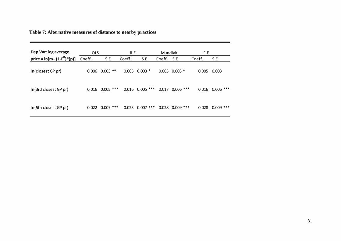
31

Table 7: Alternative measures of distance to nearby practices

Coeff. Coeff. Coeff. S.E. Coeff. S.E.

ln(closest GP pr) 0.006 0.003 ** 0.005 0.003 * 0.005 0.003 * 0.005 0.003

ln(3rd closest GP pr) 0.016 0.005 *** 0.016 0.005 *** 0.017 0.006 *** 0.016 0.006 ***

ln(5th closest GP pr) 0.022 0.007 *** 0.023 0.007 *** 0.028 0.009 *** 0.028 0.009 ***

Dep Var: log average price = ln[m+ (1‐FB)*(p)]

OLS R.E. Mundlak F.E.

S.E. S.E.

32

Appendix A We derive these results by noting that, at the Nash equilibrium, the condition (10) on p is

2112

ˆ ˆ1 ; 1 ; 0h

h F p m q Ft

so that 2112p t m q . Substituting into the condition (11) on q1 gives

1 ˆ1 ;q h F +1

ˆ( ; )

i

h f d

= 0

and so cancelling and dividing by 1 F(̂ ;θ) gives (17) and substituting (17) into the

expression for p gives (16). The condition (12) on the bulk billing threshold ̂ implies that

with an interior solution ̂ (α0,α1) the profit on the marginal patient type is the same

whether they are bulk billed or not bulk billed so that 2102m q = 21

12p m q , or using

(16), 2102m q = t , and this yields the expression (15) for q0. Condition (9) can be written

as 0ˆ1 ;q h F =

0

ˆ2102 ( ; )

ihm q f d

t

, so that cancelling h, dividing through

by (1F), and substituting for q0 from (15), gives the expression (18) for the expected value

of α for bulk billed patients.

If the Nash equilibrium has no patient being bulk billed (Fb = 0, ̂ = α0) the first order

conditions on price and quality imply

2112 0t p m q (36)

0q t 2112 0p m q (37)

where is the unconditional expectation of α. Hence we can solve for

2

2p t m

(38)

1q

(39)

If the Nash equilibrium has GPs bulk billing all their patients (Fb = 1,̂ = α1) the first order

condition on quality implies

210 02 0q t m q (40)

where is the unconditional mean of the marginal valuation of quality.