competitive learning: from interactive activation to...

COGNITIVE SCIENCE 11, 23-63 (1987)

Competitive Learning:

From Interactive Activation to

Adaptive Resonance

STEPHEN GROSSBERG

Boston University

Functional ond mechanistic comparisons are mode between several network

models of cognitive processing: competitive learning, interactive activation,

adaptive resonance, and back propagation. The starting point of this comparison

is the article of Rumelhart ond Zipser (1985) on feature discovery through compe-

titive learning. All the models which Rumelhart and Zipser (1985) have described

were shown in Grossberg (1976b) to exhibit a type of learning which is temporally

unstable. Competitive learning mechanisms con be stabilized in response to an

arbitrary input environment by being supplemented with mechanisms for learn-

ing top-down expectancies, or templates; for matching bottom-up input patterns

with the top-down expectancies; and for releasing orienting reactions in o mis-

match situation, thereby updating short-term memory ond searching for another

internal representation. Network architectures which embody all of these mecho-

nisms were called adaptive resonance models by Grossberg (1976~). Self-stabil-

izing learning models are candidates for use in real-world applications where

unpredictable changes can occur in complex input environments. Competitive

learning postulates ore inconsistent with the postulates of the interactive activo-

tion model of McClelland and Rumelhart (1981). and suggest different levels of

processing and interaction rules for the analysis of word recognition. Adaptive

resonance models use these alternative levels and interaction rules. The self-

organizing learning of on odaptive resonance model is compared ond contrasted

with the teacher-directed learning of a back propagation model. A number of

criteria for evaluating reol-time network models of cognitive processing ore

described and applied.

1. INTRODUCTION

Many cognitive scientists are now rapidly translating their intuitions about human intelligence into real-time network models. As each research group

Supported in part by the Air Force Office of Scientific Research (AFOSR 850149 and AFOSR F49620-86-C-0037) and the National Science Foundation (NSF IST-8417756).

Acknowledgements: Thanks to Cynthia Suchta for her valuable assistance in the preparation of the manuscript.

Correspondence and requests for reprints should be sent to the author at the Center for Adaptive Systems, Boston University, 111 Cummington Street, Boston, MA 02215.

23

24 GROSSBERG

injects a stream of new models into this sprawling literature, it becomes ever more essential to penetrate behind the many ephemeral differences between models to the deeper architectural level on which a formal model lives. What are the key issues, principles, properties, mechanisms, and data that may be used to distinguish one model from another? How may we decide whether two seemingly different models are really formally equivalent, or are probing profoundly different aspects of cognitive processing?

This article outlines a comparative analysis of network models within a focused conceptual domain. Its starting point is the recent article by Rumel- hart and Zipser (1985) on competitive learning models that was published in this journal as part of a special issue on connectionist models. The discus- sions raised by this article lead naturally to a comparison of several distinct models, notably competitive learning, interactive activation, adaptive resonance, and back propagation models. Before considering these models, I briefly discuss why real-time network models are so important, and why their very promise makes them difficult to understand.

2. EMERGENT PROPERTIES OF NETWORK INTERACTIONS: FUNCTION VERSUS MECHANISM

A key issue leading to network models concerns how the behavior of individ- uals adapts successfully in real-time to constaints imposed by their environments. In order to analyse this issue, one needs to identify the functional level on which an individual’s behavioral success is defined. Much theoretical and experimental evidence suggests that this is the level of neural networks, rather than the level of individual nerve cells. Key behavioral properties are often emergent properties due to interactions among many cells in a neural network. Thus, the study of real-time networks is important because behavior can best be understood on the level of a network analysis.

Often a network’s emergent properties are much more complex than the network components from which they arise. In a good network model, the whole is far greater than the sum of its parts. In addition, the formal relationships among those emergent properties may be quite subtle, and may reflect the delicate interplay of behavioral properties that are characteristic of living organisms. Thus network models can excite our interest by showing us how subtle and complex functional properties can emerge from interactions among simple components.

The very fact, however, that simple network laws can generate complex behaviors makes network models difficult to understand. In order to effec- tively analyse a network model, one needs powerful analytic and computational methods to derive the complex emergent properties of the network from a description of its simple components. A network model cannot, in

COMPETITIVE LEARNING 25

principle, be understood merely as a list of processing rules or as a computer program. In order to adequately describe the dynamism of such a network, it is necessary to use a mathematical formalism that can naturally analyse interactions which may occur in a nonlinear fashion across thousands or even millions of components. The need for such a formal analysis is especially great when the network can learn, since the same laws define the network at all times, but its functional properties may be radically different before and after learning occurs.

The distinction between a network’s emergent functional properties and its simple mechanistic laws also clarifies why the controversy surrounding the relationship of an intelligent system’s abstract properties to its mechanistic instantiation has been so enduring. Without a linkage to mechanism, a network’s functional properties cannot be formally or physically explained. On the other hand, how do we decide which mechanisms are crucial for generating desirable functional properties and which mechanisms are adventi- tious? Two seemingly different models can be equivalent from a functional viewpoint if they both generate similar sets of emergent properties. An analysis which proves such a functional equivalence between models does not, however, minimize the importance of their mechanistic descriptions. Rather, such an analysis identifies mechanistic variations which are not likely to be differentiated by evolutionary pressures which select for these functional properties on the basis of behavioral success.

Another side of such an evolutionary analysis concerns the identification of the fundamental network modules which are specialized by the evolutionary process for use in a variety of behavioral tasks. How do evolutionary variations of a single network module, or blueprint, generate behavioral properties which, on the level of raw experience, seem to be phenomenally different and even functionally unrelated? Although each specialized network may generate a characteristic bundle of emergent properties, para- metric changes of these specialized networks within the framework of a single network may generate bundles of emergent properties that are qualitatively different. In order to identify the mechanistic unity behind this phenom- enal diversity, appropriate analytic methods are once again indispensable.

In summary, the relationship between the emergent functional properties that govern behavioral success and the mechanisms that generate these properties is far from obvious. A single network module may generate qualitatively different functional properties when its parameters are changed. Conversely, two mechanisms which are mechanistically different may generate formally homologous functional properties. The intellectual difficulties caused by these possibilities are only compounded by the fact that we are designed by evolution to be serenely ignorant of our own mechanistic substrates. The very cognitive ad learning mechanisms which enable us to group, or chunk, ever more complex information into phenomenally simple unitized represen-

26 GROSSBERG

tations act to hide from us the myriad interactions that subserve these representations during every moment of experience. Thus we cannot turn to our daily intuitions or to our lay language for secure guidance in discovering or analysing network models. The simple lesson that the whole is greater than the sum of its parts forces us to use an abstract mathematical language that is capable of analysing interactive emergence and functional equivalence.

3. PROCESSING LEVELS AND INTERACTIONS: MODELS OR METAPHORS?

A network model is usually easy to define using just a few equations. These equations specify the dynamical laws governing the model’s nodes, or cells, including the processing levels in which these nodes are embedded. The equations also specify the interactions between these nodes, including which nodes are connected by pathways and the types of signals or other processes that go on in these pathways. Inputs to the network, outputs from the network, parameter choices within the network, and initial values of network variables often complete the model description. Such components are common to essentially all real-time network models. Thus, to merely say that a model has such components is scientifically vacuous.

How, then, can we decide when a network model is wrong? Such a task is deceptively simple. If the model’s levels are incorrectly chosen, then it is wrong. If its interactions are incorrectly chosen, then it is wrong. And so on. The only escape from such a critique would be to demonstrate that a different set of levels and interactions can be correctly chosen, and shares similar functional properties with the original model. The new choice of levels and interactions would, however, constitute a new model. The old model would still be wrong. Such an analysis would show that the shared model properties are essentially model-independent, yet that there exist finer tests to distinguish between models. I will describe several such tests below.

In the absence of such a literal process of model selection and rejection, it would soon become impossible to criticize a model at all, since its authors could claim that they really did not intend their model to be literally interpreted. To avoid criticism or disconlirmation, the model could be turned into a metaphor of itself, or even into a vaguely outlined framework that could be broadly enough defined to include all future modeling possibilities, including possibilities that flatly contradicted the original model.

McClelland (1985, p. 144) essentially advocated this position when he wrote “we would not view the interactive activation model as a description of a mechanism at ah. . .it allows us to study interactive activation models of a wide range of phenomena at a psychological or functional level without


necessarily worrying about the plausibility of assuming that they provide an adequate description of the actual implementation.” As noted above, dis- sociation of a functional description from a mechanistic description is impossible in a network model. The possibility that a particular mechanistic instantiation may be functionally equivalent to a different instantiation does not in the least free us from committing ourselves to particular classes of mechanisms. McClelland’s usage would become acceptable only if we agreed to use the term “interactive activation” model to mean any real-time network model. Such a usage would, however, make the term scientifically vacuous. In addition, the interactive activation model is a relatively recent member of the family of real-time network models in psychology. It has added no new qualitative concepts to this class of models US a framework, hence it needs to be analysed as a model in order to appreciate its contribution to the network modeling literature. All models discussed in this article will be treated literally as models, rather than as metaphors or frameworks of models.

4. FEATURE DISCOVERY BY COMPETITIVE LEARNING

I will use the Rumelhart and Zipser (1985) article to motivate my analysis of a number of issues which promise to play a central role in evaluating the strengths and weaknesses of various network models. Rurnelhart and Zipser (1985) analyse a type of learning model which is called a competitive learning model. They acknowledge that competitive learning models have been intensively studied for some time and thus conclude that “it seems reason- able to put the whole issue into historical perspective” (p. 76). They also note that “It is a common practice to handcraft networks to carry out particular tasks. Whenever one creates such a network that performs a task rather successfully, the question arises as to how such a network might have evolved. The word perception model developed in McClelland and Rumel- hart (1981) and Rumelhart and McClelland (1982) is one such case in point. That model offers rather detailed accounts of a variety of word perception experiments, but it was crafted to do its job. How could it have evolved naturally? Could a competitive learning mechanism create such a network?” (p. 98). Thus, these authors ask how a competitive learning networkcan be joined to an interactive activation network in order to endow the latter type of network with a learning capability.

Their discussion does not, however, acknowledge that both the levels and the interactions of a competitive learning model are incompatible with those of an interactive activation model (Grossberg, 1984). The authors likewise do not state that the particular competitive learning model which they have primarily analysed is identical to the model introduced and analysed in

28 GROSSBERG

Grossberg (1976a, 1976b), nor that this model was consistently embedded into an adaptive resonance model in Grossberg (1976~) and later developed in Grossberg (1978) to articulate the key functional properties which McClel- land and Rumelhart described when they introduced the interactive activation model in McClelland and Rumelhart (1981). In summary, the stated goal of Rumelhart and Zipser (1985)-to join a competitive learning model with a model capable of generating functional properties that are shared with the interactive activation model-was carried out using an adaptive resonance model in Grossberg (1978). In addition, the interactive activation model US a model is incapable of participating in such a synthesis.

The Rumelhart and Zipser (1985) article thus raises a number of issues which make real-time network models so difficult to understand and to dif- ferentiate. How can an adaptive resonance model share functional properties with an interactive activation model, yet be mechanistically consistent with a competitive learning model with which the interactive activation model is mechanistically inconsistent? What design principles are realized by an adaptive resonance model but not by an interactive activation model which can be used to distinguish these models on a deep computational level? The analysis of Rumelhart and Zipser (1985) provides no light into these matters. Indeed, these authors also stated that “our analyses differ from many of these [former analyses] in that we focus on the development of feature detectors rather than pattern classification” (p. 76). A glance at such titles as Malsburg (1973) and Grossberg (1976a, 1976b) shows that this observation is also inaccurate.

5. THE PROBLEM OF TEMPORALLY UNSTABLE LEARNING

Analysis of the competitive learning model revealed a fundamental problem which is shared by most other learning models that are now being developed and which was overcome by the adaptive resonance theory. I will now illustrate this general problem using a competitive learning model, before indi- cating that adaptive variants of the interactive activation model cannot solve it.

The particular competitive learning models described in Grossberg (1976b) and in Rumelhart and Zipser (1985) were used to show how a stream of input patterns to a network level F, can adaptively tune the weights, or long term memory (LTM) traces, in the pathways from F, to a coding level F2. Although these L.7” traces may initially be randomly chosen, the presentation of inputs at F, can alter the LTM traces through learning in such a way that F, eventually parses the input patterns into sets which activate distinct recognition categories. Appendix 1 describes this competitive learning scheme as well as the formal identity of the Grossberg (1976b) model with the model studied by Rumelhart and Zipser (1985).


In Grossberg (1976b), a theorem was proved which described input environments to which the model responds by learning a temporally stable recognition code. This theorem is described in Appendix 2. The theorem proved that, if not too many input patterns are presented to F,, relative to the number of coding nodes in F2, or if the input patterns form not too many clusters, then learning of the recognition code eventually stabilizes. In addition, the learning process elicits the best distribution of LTMtraces that is consistent with the structure of the input environment. The computer simulations of Rumelhart and Zipser (1985) essentially confirm this theorem.

Despite the demonstration of input environments that can be stably coded, it was also shown, through explicit counterexamples, that a competitive learning model cannot learn a temporally stable code in response to arbitrary input environments. Moreover, these counterexamples included input environments that could easily occur in many important applications. In these counterexamples, as a list of input patterns perturbed level F, through time, the response of level F2 to the same input pattern could be different on each successive presentation of that input pattern. Moreover, the F2 response to a given input pattern might never settle down as learning proceeded.

Such unstable learning in response to a prescribed input is due to the learning that occurs in response to the other, intervening, inputs. In other words, the network’s adaptability, or plasticity, enables prior learning to be washed away by more recent learning in response to a wide variety of input environments. Carpenter and Grossberg (1987a, 1987b) have extended this instability analysis by describing infinitely many input environments in which periodic presentation of just four input patterns can cause temporally unstable learning. This instability problem is not, moreover, peculiar to competitive learning models. As I shall indicate below, it is a problem of almost all learning models that are now being developed.

6. THE STABILITY-PLASTICITY DILEMMA: SELF-STABILIZED LEARNING IN A COMPLEX

AND CHANGING ENVIRONMENT

This instability problem was too fundamental to be ignored. In addition to showing that learning could become unstable in response to a complex input environment, the analysis also showed that learning could alI too easily become unstable due to simple changes in an input environment. Changes in the probabilities of inputs, or in the deterministic sequencing of inputs, could readily wash away prior learning.

The seriousness of this problem can be dramatized by imagining that you have grown up in Boston before moving to Los Angeles, but periodically return to Boston to visit your parents. Although you may need to learn many new things to enjoy life in Los Angeles, these new learning experiences

30 GROSSBERG

do not prevent you from knowing how to find your parent’s house or otherwise remembering Boston. A multitude of similar examples illustrate that we are designed to successfully adapt to environments whose rules may change-without necessarily forgetting our old skills. Moreover, we are designed to successfully adapt to environments whose rules may change un- predictably, and can do so even if no one tells us that the environment has changed. We can adapt, in short, without a teacher, and through a direct confrontation with our experiences. Such adaptation is called self-organization in the network modeling literature.

The instability of the competitive learning model thus emphasized the fundamental nature of the stability-plasticity dilemma (Grossberg, 1980, 1982a, 1982b): How can a learning system be designed to remain plastic in response to significant new events, yet also remain stable in response to irrelevant events? How does the system know how to switch between its stable and its plastic modes in order to prevent the relentless degradation of its learned codes by the “blooming buzzing confusion” of irrelevant experience? How can it do so without using a teacher? The problem addresses one of the key capabilities that makes a human cognitive system so remarkable: its ability to learn internal representations of awesome amounts of the widest possible variety of environmental stimuli in real-time and without a teacher. The stability-plasticity dilemma articulates one sense in which a cognitive system is universal. Unlike the individual senses, which are specialized to deal with particular classes of inputs, a cognitive system is designed to integrate unanticipated combinations of events from all the senses into coherent moments of resonant recognition.

Rumelhart and Zipser (1985) were able to ignore this fundamental issue by considering simple input environments whose probabilistic rules do not change through time. Other modelers, for example, Kohonen (1984), have stabilized learning in their applications of the competitive learning model by externally shutting off plasticity before the learned code can be erased. This approach creates the danger of shutting off plasticity too soon, in which case important information is not learned, or too late, in which case important learned information can be erased. The only way to overcome instability using this approach in an unpredictable input environment is to assume that the observer, or teacher, who shuts off plasticity is omniscient. If a model of an omniscient teacher is available, however, then you will not also need a model of a potentially unstable learning process.

Yet other modelers, such as Ackley, Hinton, and Sejnowski (1985), Hop- field (1982), Knapp and Anderson (1984), McClelland and Rumelhart (1985), Rumelhart, Hinton, and Williams (1986), and Sejnowski and Rosenberg (1986), have stabilized their models by externally restricting the input environment. They thereby recast the problem of model instability into one about model capacity: What sorts of restricted input environments can


these models handle before their learned codes are washed away by the flux of input experience? None of these learning models has yet addressed the general instability problem that was articulated a decade ago.

7. THE INCOMPATIBILITY OF THE COMPETITIVE LEARNING AND INTERACTIVE ACTIVATION MODELS:

LETTER AND WORD LEVELS DO NOT EXIST

Before outlining a solution of the stability-plasticity dilemma, I indicate the nature of the inconsistency between the competitive learning model and the interactive activation model. Both the levels and the interactions of the two models are incompatible.

In a competitive learning model, all interactions between levels are excitatory. The only inhibitory interactions occur within each level. By contrast, in the Rumelhart and McClelland (1982, p. 61) model “Each letter node is assumed to activate all of those word nodes consistent with it and inhibit all other word nodes.” Thus, the two models postulate different types of inter- level interactions. The selective activations and inhibitions that are hypothe- sized to exist between consistent and inconsistent letter nodes and word nodes must obviously be learned. In Grossberg (1984), it was shown that such connections cannot be learned using competitive learning mechanisms. Thus the postulated connections from letter nodes to word nodes are inconsistent, in a fundamental way, with competitive learning mechanisms.

An equally serious issue concerns the fact that the letter level and the word level which are postulated in the interactive activation model do not exist either in a language learning model that is based upon competitive learning mechanisms or, I would claim, in vivo. Instead, these levels code what I have called items and lists, respectively (Cohen & Grossberg, 1986; Gross- berg, 1978, 1982a, 1984; 1987b; Grossberg & Stone, 1986). This insight is hinted at in the simulations which Rumelhart and Zipser (1985) have per- formed on lists of letters. These simulations are inconsistent with the existence of a letter level and a word level because both letters and words can have representations on both levels F, and F2.

The difference between levels built up from letters and words and levels built up from items and lists can begin to be appreciated through the following observations (Grossberg, 1984). McClelland and Rumelhart (1981) postulated that a stage of letter nodes precedes a stage of word nodes. They used these stages to discuss the processing of letters in Cletter words. The hypothesis of separate stages for letter and word processing implies that letters are not also represented on the level of words of length four. In order to be of general applicability, these concepts should certainly be generalizable to words of length less than four, notably to l-letter words such as A and I. A consistent extension of the McClelland and Rumelhart stages would require

32 GROSSBERG

that those letters which are also words, such as A and 1, are represented on both the letter level and the word level, whereas those letters which are not words, such as E and F, are represented only on the letter level. How this distinction could be learned by an unsupervised learning model remains unclear.

This problem of processing units is symptomatic of a more general diffi- culty. The letter and word levels contain only nodes that represent letters and words. What did these nodes represent before their respective letters and words were learned? Where will the nodes come from to represent the letters and words that the model individual has not yet learned? Are these nodes to be created de novo? They certainly cannot be created de novo within the five or six trials that enable a pseudoword to acquire many of the recognition characteristics of a word (&lasso, Shiffrin, & Feustel, 1984)? These concerns clarify the need to define a processing substrate that can represent the learned units of a subject’s internal lexicon before, during, or after they are learned.

The assumption of separate letter and word levels also requires special assumptions to deal with various data, such as the data of Wheeler (1970) and Samuel, van Santen, and Johnston (1982, 1983) concerning the word superiority effect. If separate letter and word levels exist, then letters such as A and Zwhich are also words should, as words, be able to prime their letter representations. In constrast, letters such as D and E which are not words should receive no significant priming from the word level. One might therefore expect easier recognition of A and I than of D and E. Wheeler (1970) showed that this is not the case.

The assumptions of separate letter and word levels could escape this con- tradiction by assuming that all letters can be recognized so much more quickly than words of length at least two that no priming whatsoever can be received from the word level before letter recognition is complete. This assumption seems to be incompatible with the word length data of Samuel, van Santen, and Johnston (1982, 1983). These authors showed that recognition im- proves if a letter is embedded in words of greater length. Thus a letter that is presented alone for a fixed time before a mask appears is recognized less well than a letter presented for the same amount of time in a word length 2, 3, or 4. These data cast doubt on any explanation based on speed of processing alone, since they suggest that priming of letters due to multiletter words is effective.

In contrast, within a model which uses a item level and a list level, all familiar letters possess both item and list representation, not just letters such as A and I that are also words. Thus a model which uses an item level and a list level can readily explain the Wheeler (1970) data. An analysis of how item and list representations are built up led, in fact, to the prediction of a word length effect for words of lengths 1,2,3, and 4 (Grossberg, 1978,


Section 41; reprinted in Grossberg, 1982a). Cohen and Grossberg (1986a, 1987b) describe computer simulations of how item and list levels interact.

8. ADAPTIVE RESONANCE THEORY: SELF-STABILIZATION OF CODE LEARNING IN AN

ARBITRARY INPUT ENVIRONMENT

A formal analysis of how to overcome the learning instability experienced by a competitive learning model led to the introduction of an expanded theory, called adaptive resonance theory (ART), in Grossberg (1976c). This formal analysis showed that a certain type of top-down learned feedback and matching mechanism could significantly overcome the instability problem. It was also realized that top-down attentional mechanisms, which had earlier been discovered through an analysis of interactions between cognitive and reinforcement mechanisms (Grossberg, 1973, had the same properties as these code-stabilizing mechanisms. In other words, once it was recognized how to formally solve the instability problem, it also became clear that one did not need to invent any qualitatively new mechanisms to do so. One only needed to remember to include previously discovered attentional mechanisms! These additional mechanisms enable code learning to self-stabilize in response to an essentially arbitrary input environment. For a recent mathematical proof of this type of stability, see Carpenter and Grossberg (1987b).

The types of top-down effects, such as the “rich-get-richer” and “gang” effects, which McClelland and Rumelhart (1981) experimentally reported were predicted formal properties of the ART theory as developed in Gross- berg (1978). Such properties are shared by many networks which undergo reciprocal bottom-up and top-down feedback exchanges. They arose in ART as predictions about the emergent properties of network architectures that were designed to guarantee self-stabilizing self-organization of cognitive recognition codes-the very properties that are absent from the interactive activation model. In addition to such properties, ART has by now been used to analyse and predict data about speech perception, word recognition and recall, visual perception, olfactory coding, classical and instrumental conditioning, decision making under risk, event related potentials, neural substrates of learning and memory, critical period termination, and amnesias (Banquet & Grossberg, 1987; Carpenter & Grossberg, 1987a, 1987b, 1987c; Cohen & Grossberg, ;1987a, 1987b; Grossberg, 1982b, 1984, 1987a, 1987b; Grossberg & Gutowski, 1987; Grossberg & Levine, 1987; Grossberg & Stone, 1986a, 1986b). Thus ART has already demonstrated an explanatory and predictive competence as an interdisciplinary physical theory. It is now being developed both to expand its predictive range and to implement it in real-time hardware. In Sections 9-15, some properties of ARTare outlined as a basis for comparisons with other learning models in the literature, such

34 GROSSBERG

as the back propagation model. These comparisons delineate issues that could just as easily be raised in the evaluation of any network learning model.

9. SOLVING THE STABILITY-PLASTICITY DILEMMA USING INTERACTING ATTENTIONAL AND ORIENTING SYSTEMS

In addition to the bottom-up mechanisms of a competitive learning model, an ARTsystem includes processes for learning of top-down expectancies, or templates; for matching bottom-up input patterns with top-down expectancies; and for releasing orienting reactions in a mismatch situation, thereby leading to rapid updating, or reset, of short term memory as the network carries out a hypothesis testing scheme that searches for and, if necessary, leads to learning of a better representation of the input pattern (Figure 1).

Using these mechanisms, an ART system can generate recognition codes adaptively, and without a teacher, in response to a series of environmental inputs. As learning proceeds, interactions between the inputs and the system generate new steady states, or equilibrium points. The steady states are formed as the system discovers and learns critical featurepatterns, or prototypes, that represent invariants of the set of all experienced input patterns. These learned codes are dynamically buffered, or stabilized, against relentless recoding by irrelevant inputs. The formation of steady states is internally controlled using mechanisms that suppress possible sources of system instability.

An ART system can adaptively switch between its stable and plastic modes. It is capable of plasticity in order to learn about significant new events, yet it can also remain stable in response to irrelevant events. In order to make this distinction, an ARTsystem is sensitive to novelty. It is capable, without a teacher, of distinguishing between familiar and unfamiliar events, as well as between expected and unexpected events.

Multiple interacting memory systems are needed to monitor and adaptively react to the novelty of events without an external teacher. Within ART, interactions between two functionally complementary subsystems are used to process familiar and unfamiliar events. Familiar events are processed within an attentional subsystem, which is built up from a competitive learning network. The attentional subsystem establishes ever more precise internal representations of and responses to familiar events. It also learns the top-down expectations that help to stabilize the learned bottom-up codes of familiar events. As described above, however, the attentional subsystem is unable simultaneously to maintain stable representations of familiar categories and to create new categories for unfamiliar patterns in certain input environments. An isolated attentional subsystem can become either too rigid and incapable of creating new categories for unfamiliar patterns, or too unstable and capable of ceaselessly recoding the categories of familiar patterns as the statistics of the input environment change.

COMPETITIVE LEARNING

ATTENTIONAL ORIENTING SUBSYSTEM SUBSYSTEM

GAIN CON-lROL DIPOLE FIELD

GAIN CONTROL -

+ +

I

35

INPUT PATTERN

Figure 1. Anatomy of the ottentional-orienting system: Two successive stages, F, and 15, of

the attentional subsystem encode patterns of activation in short term memory (STM).

Bottom-up ond top-down pathways between FI and 15 contain adaptive long term memory

(LTM) traces which multiply the signols in these pathways. The remainder of the circuit

modulates these STM ond LTM processes. Modulation by gain control enables F, to distin-

guish between bottom-up input patterns and top-down priming, or template, patterns, as

well as to match these bottom-up ond top-down patterns. Gain control signals also enoble

F, to react supraliminally to signals from F, while an input pattern is on. The orienting sub-

system A generates o reset wave to F, when mismatches between bottom-up and top-down

patterns occur ot FI. This reset wave selectively and enduringly inhibits active h cells until

the input is shut off. (Reprinted with permission from Carpenter and Grossberg, 1987b).

The second subsystem is an orienting subsystem that resets the attentional subsystem when an unfamiliar event occurs. Interactions between the attentional subsystem and the orienting subsystem help to express whether a novel pattern is familiar and well represented by an existing recognition code, or unfamiliar and in need of a new recognition code (Figure 1). Within an ART system, attentional mechanisms play a major role in self- stabilizing the learning of an emergent recognition code. A mechanistic analysis of the role of attention in learning has led Carpenter and Grossberg (1987a, 1987b) to distinguish between four types of attentional mechanisms attentional priming, attentional gain control, attentional vigilance, and in- termodality competition (see Figure 4).

34 GROSSBERG

10. SELF-SCALING COMPUTATIONAL UNITS, SELF-ADJUSTING MEMORY SEARCH, DIRECT ACCESS,

AND ATTENTIONAL VIGILANCE

Four properties are basic to the workings of an ARTnetwork. Violating any one of these properties prevents the network from learning well in certain input environments. Essentially all other learning models violate one or more of these properties.

A. Self-Scaling Computational Units: Critical Feature Patterns Properly defining signal and noise in a self-organizing system raises a number of subtle issues. Pattern context must enter the definition so that input features which are treated as irrelevant noise when they are embedded in a given input pattern may be treated as informative signals when they are embedded in a different input pattern. The system’s unique learning history must also enter the definition so that portions of an input pattern which are treated as noise when they perturb a system at one stage of its self-organization may be treated as signals when they perturb the same system at a different stage of its self-organization. The present systems automatically self-scale their computational units to embody context- and learning-dependent defi- nitions of signal and noise.

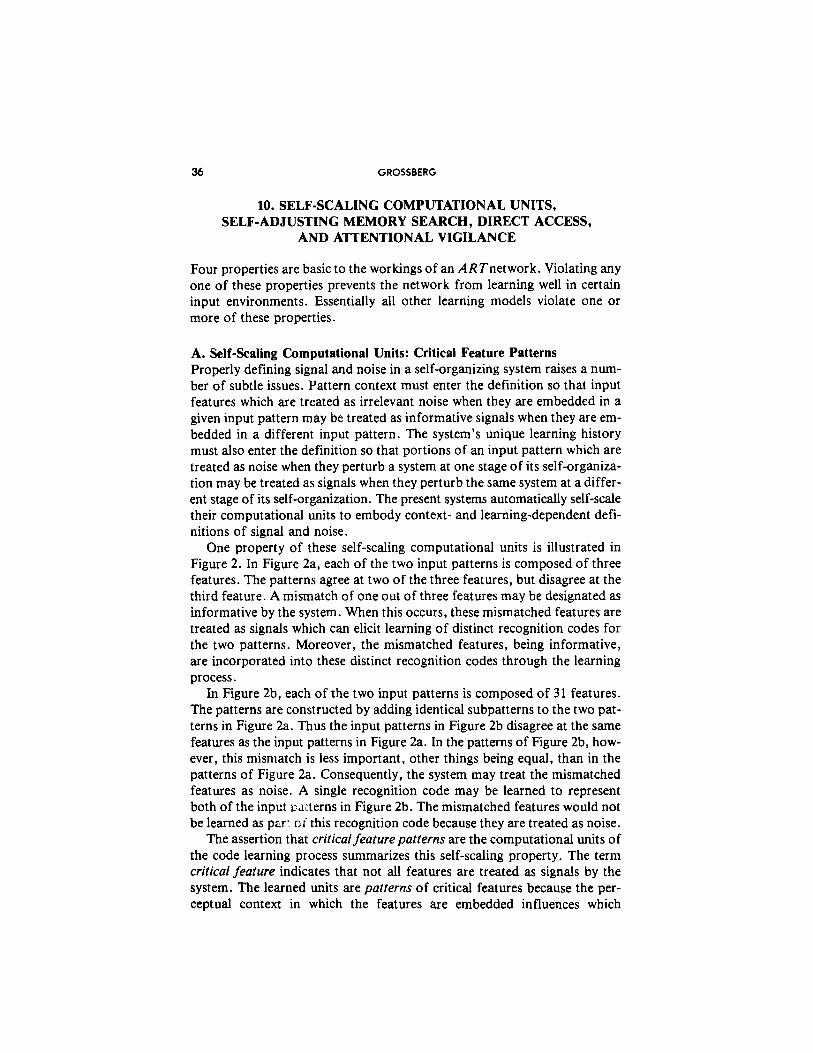
One property of these self-scaling computational units is illustrated in Figure 2. In Figure 2a, each of the two input patterns is composed of three features. The patterns agree at two of the three features, but disagree at the third feature. A mismatch of one out of three features may be designated as informative by the system. When this occurs, these mismatched features are treated as signals which can elicit learning of distinct recognition codes for the two patterns. Moreover, the mismatched features, being informative, are incorporated into these distinct recognition codes through the learning process.

In Figure 2b, each of the two input patterns is composed of 31 features. The patterns are constructed by adding identical subpatterns to the two patterns in Figure 2a. Thus the input patterns in Figure 2b disagree at the same features as the input patterns in Figure 2a. In the patterns of Figure 2b, however, this mismatch is less important, other things being equal, than in the patterns of Figure 2a. Consequently, the system may treat the mismatched features as noise. A single recognition code may be learned to represent both of the input cclrterns in Figure 2b. The mismatched features would not be learned as par: ci this recognition code because they are treated as noise.

The assertion that critical feature patterns are the computational units of the code learning process summarizes this self-scaling property. The term critical feature indicates that not all features are treated as signals by the system. The learned units are patterns of critical features because the perceptual context in which the features are embedded influences which


ibj

F;t n

Figure 2. Self-scaling property discovers critical features in r~ context-sensitive way: (a)

Two input patterns of 3 features mismatch at 1 feature. When this mismatch is sufficient to

generate distinct recognition codes for the two patterns, the mismatched features are en-

coded in LTM as part of the critical feature patterns of these recognition codes. (b) Identical

subpatterns are added to the two input patterns in (a). Although the new input patterns

mismatch at the same one feature, this mismatch may be treated as noise due to the addi-

tional complexity of the two new patterns. Both patterns moy thus learn to activate the

same recognition code. When this occurs, the mismatched feature is deleted from LTM in

the critical feature pattern of the code.

features will be processed as signals and which features will be processed as noise. Thus a feature may be a critical feature in one pattern (Figure 2a) and an irrelevant noise element in a different pattern (Figure 2b).

B. Self-Adjusting Memory Search No pre-wired search algorithm, such as a search tree, can maintain its efficiency as a knowledge structure evolves due to learning in a unique input environment. A search order that may be optimal in one knowledge domain may become extremely inefficient as that knowledge domain becomes more complex due to learning.

An ARTsystem is capable of a parallel memory search that adaptively up- dates its search order to maintain efficiency as its recognition code becomes arbitrarily complex due to learning. This self-adjusting search mechanism is part of the network design whereby the learning process self-stabilizes by engaging the orienting subsystem.

None of these mechanisms is akin to the rules of a serial computer program. Instead, the circuit architecture as a whole generates a self-adjusting search order and self-stabilization as emergent properties that arise through system interactions. Once the ART architecture is in place, a little random- ness in the initial values of its memory traces, rather than a carefully wired search tree, enables the search to carry on until the recognition code self- stabilizes.

C. Direct Access to Learned Codes A hallmark of human recognition performance is the remarkable rapidity with which familiar objects can be recognized. The existence of many learned

38 GROSSBERG

recognition codes for alternative experiences does not necessarily interfere with rapid recognition of an unambiguous familiar event. This type of rapid recognition is very difficult to understand using models wherein trees or other serial algorithms need to be searched for longer and longer periods as a learned recognition code becomes larger and larger.

In an ART model, as the learned code becomes globally self-consistent and predictively accurate, the search mechanism is automatically disengaged. Subsequently, no matter how large and complex the learned code may become, familiar input patterns directly uccess, or activate, their learned code, or category. Unfamiliar patterns can also directly access a learned category if they share invariant properties with the critical feature pattern of the category. In this sense, the critical feature pattern acts as a prototype for the entire category. As in human pattern recognition experiments, a “prototype” input pattern that perfectly matches a learned critical feature pattern may be better recognized than any of the “exemplar” input patterns that gave rise to the critical feature pattern (Posner, 1973; Posner & Keele, 1968, 1970). Grossberg and Stone (1986a) have shown, moreover, that these direct access properties can be used to explain R T and error data from lexical decision and word familiarity experiments.

Unfamiliar input patterns which cannot stably access a learned category engage the self-adjusting search process in order to discover a network substrate for a new recognition category. After this new code is learned, the search process is automatically disengaged and direct access ensues.

We use the term critical feature pattern, rather than prototype, because critical feature patterns are learned, matched, and regulate future learning in a manner different from classical prototype models. Estes (1986) compared several types of category learning models in the light of recent data and showed that exemplar models, prototype models, and exemplar similarity models all have their merits. An ART model can also be sensitive to exemplars, prototypes, or similarity between exemplars, depending upon the experimental conditions. One factor that mediates between these alternatives is now summarized.

D. Environment as a Teacher: Modulation of Attentional Vigilance Although an ART system self-organizes its recognition code, the environment can also modulate the learning process and thereby carry out a teaching role. This teaching role allows a system with a fixed set of feature detectors to function successfully in an environment which imposes variable performance demands. Different environments may demand either coarse discriminations or fine discriminations to be made among the same set of objects.

In an ART system, if an erroneous recognition is followed by an environmental disconfirmation, such as a punishment, then the system becomes more vigilant. This change in vigilance may be interpreted as a change in the sys-


tern’s attentional state which increases its sensitivity to mismatches between bottom-up input patterns and active top-down critical feature patterns. A vigilance change alters the size of a single parameter in the network. The interactions within the network respond to this parameter change by learning recognition codes that make finer distinctions. In other words, if the network erroneously groups together some input patterns, then negative reinforcement can help the network to learn the desired distinction by making the system more vigilant. The system then behaves us ifit has a better set of feature detectors. Thus at a level of very high vigilance, a category may emerge that accepts only one exemplar. At lower levels of vigilance, similarity relationships among the accepted exemplars help to mold the category’s emergent critical feature pattern. Different vigilance levels may, moreover, be imposed by environmental feedback in response to easy or difficult discriminations during the course of a single experiment or experience.

The ability of a vigilance change to alter the course of pattern recognition illustrates a theme that is common to a variety of neural processes: a one- dimensional parameter change that modulates a simple nonspecific neural process can have complex specific effects upon high-dimensional neural information processing.

11. BOTTOM-UP ADAPTIVE FILTERING AND CONTRAST-ENHANCEMENT IN SHORT-TERM MEMORY

The typical network reactions to a single input pattern I within a temporal stream of input patterns are now briefly summarized. Each input pattern may be the output pattern of a preprocessing stage. Different preprocessing is given, for example, to speech signals and to visual signals before the out- come of such modality-specific preprocessing ever reaches the attentional subsystem. The preprocessed input pattern I is received at the stage F, of an attentional subsystem. Pattern I is transformed into a pattern X of activation across the nodes, or abstract “feature detectors”, of F, (Figure 3). The transformed pattern X is said to represent I in short term memory (STM). In F, each node whose activity is sufficiently large generates excitatory signals along pathways to target nodes at the next processing stage F,. A pattern X of STM activities across F, hereby elicits a pattern S of output signals from F, . When a signal from a node in F, is carried along a pathway to F2, the signal is multiplied, or gated, by the pathway’s long term memory (LTM) trace. The LTM gated signal (i.e., signal times LTM trace), not the signal alone, reaches the target node. Each target node sums up all of its LTM gated signals. In this way, pattern S generates a pattern T of LTM- gated and summed input signals to F2 (Figure 4a). The transformation from S to T is called an adaptive jilter.

GROSSBERG

F 2

F 1

STM ACTIVITY PATTERN (Y)

‘j u

Xi)

vi l

SlTVl ACTIVITY PATTERN

l vM. w> A

I T T T T 4

INPUT PATTERN (I) Figure 3. Stages of bottom-up activation: The input pattern I generotes a pattern of STM ac-

tivation Xacross FI. Sufficiently active FI nodes emit bottom-up signals to 6. This signal pat-

tern S is gated by long term memory (LTM) traces within the 6--F, pathways. The LTM gated

signals are summed before activating their target nodes in F,. This LTM-gated and summed

signal pattern T generates a pottern of activation Y across Fr. The nodes in F, are denoted

by VI, vs. ,VM. The nodes in F1 are denoted by VM+I, VM+~, VN. The input to node VI is

denoted by II. The STM activity of node VI is denoted by XI. The LTM trace of the pathway

from VI to VI is denoted by 11,.

The input pattern Tto F2 is quickly transformed by interactions among the nodes of Fr. These interactions contrast-enhance the input pattern T. The resulting pattern of activation across F, is a new pattern Y. The contrast-enhanced pattern Y, rather than the input pattern T, is stored in STM by F2. These interactions also occur in a competitive learning model.

12. TOP-DOWN TEMPLATE MATCHING AND STABILIZATION OF CODE LEARNING

As soon as the bottom-up STM transformation X- Y takes place, the STM activities Y in F2 elicit a top-down excitatory signal pattern I/ back to F,


T

t S

I

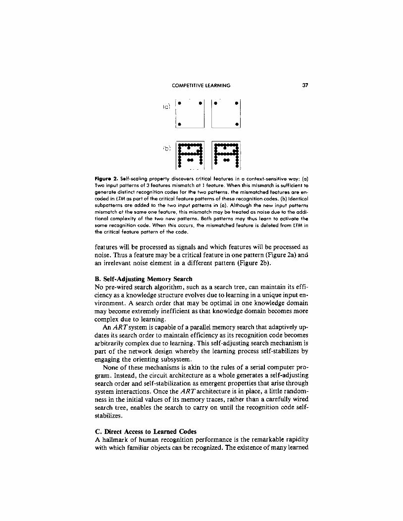
Figure 4. Search for a correct 15 code: (a) the input pattern I generates the specific STM ac-

tivity pattern X at F, OS it nonspecifically activates A. Pattern X both inhibits A and gen-

erates the output signal pattern S. Signal pattern S is tronsformed into the input pottern T,

which activates the STM pattern Y across F,. (b) Pattern Y generates the top-down signal

pattern U which is transformed into the template pattern V. If V mismatches I at Ft. then a

new STM activity pottern X’ is generoted at F,. The reduction in totol STM activity which oc-

curs when X is transformed into X’ causes a decrease in the total inhibition from FI to A.

(c) Then the input-driven activation of A con release a nonspecific arausol wove in Fz, which

resets the STM pattern Y at F,. (d) After Y is inhibited, its top-down template is eliminoted,

and X can be reinstated ot F,. Now X once again generates input pattern T to F,, but since Y

remains inhibited T con activate o different STM pattern Y’ at Fz. If the top-dawn template

due to Y’ olsa mismatches I ot F,, then the rapid search for on appropriate F, code continues.

(Figure 4b). Only sufficiently large STM activities in Y elicit signals in U along the feedback pathways F,- F,. As in the bottom-up adaptive filter, the top-down signals I/ are also gated by LTM traces and the LTM-gated signals are summed at F, nodes. The pattern U of output signals from F, hereby generates a pattern Vof LTMgated and summed input signals to F,. The transformation from Uto Vis thus also an adaptive filter. The pattern V is called a top-down template, or learned expectation.

42 GROSSBERG

Two sources of input now perturb F,: the bottom-up input pattern Z which gave rise to the original activity pattern X, and the top-down template pattern V that resulted from activating X. The activity pattern P across F, that is induced by Z and V taken together is typically different from the activity pattern X that was previously induced by I alone. In particular, F, acts to match V against I. The result of this matching process determines the future course of learning and recognition by the network.

The entire activation sequence

I-X-S-T-Y-U-V-X* (1)

takes place very quickly relative to the rate with which the LTM traces in either the bottom-up adaptive filter S- T or the top-down adaptive filter CJ- V can change. Even though none of the LTM traces changes during such a short time, their prior learning strongly influences the STh4 patterns Y and X* that evolve within the network by determining the transformations S - T and U- V. 1 now sketch how a match or mismatch of Z and Vat F, regulates the course of learning in response to the pattern I, and in particular solves the stability-plasticity dilemma.

13. INTERACTIONS BETWEEN ATTENTIONAL AND ORIENTING SUBSYSTEMS: STM RESET AND SEARCH

In Figure 4a, as input pattern I generates an ST&l activity pattern X across F, . The input pattern Z also excites the orienting subsystem A, but pattern X at F, inhibits A before it can generate an output signal. Activity pattern X also elicits an output pattern S which, via the bottom-up adaptive filter, in- states an STh4 activity pattern Y across F2. In Figure 4b, pattern Y reads a top-down template pattern V into F,. Template V mismatches input Z, thereby significantly inhibiting STM activity across F,. The amount by which activity in X is attenuated to generate X* depends upon how much of the input pattern Z is encoded within the template pattern V.

When a mismatch attenuates STM activity across F,, the total size of the inhibitory signal from F, to A is also attenuated. If the attenuation is sufficiently great, inhibition from F, to A can no longer prevent the arousal source A from firing. Figure 4c depicts how disinhibition of A releases an arousal burst to F2 which equally, or nonspecifically, excites all the F2 cells. The cell populations of F2 react to such an arousal signal in a state-dependent fashion. In the special case that F2 chooses a single population for STM storage, the arousal burst selectively inhibits, or resets, the active population in F2. This inhibition is long-lasting. One physiological design for F2 processing which has these properties is a gated dipole field (Grossberg, 1982a, 1987a). A gated dipole field consists of opponent processing channels which are gated by habituating chemical transmitters. A nonspecific arousal


burst induces selective and enduring inhibition of active populations within a gated dipole field.

In Figure 4c, inhibition of Y leads to removal of the top-down template V, and thereby terminates the mismatch between Z and V. Input pattern Z can thus reinstate the original activity pattern X across F,, which again generates the output pattern S from F, and the input pattern Tto F2. Due to the enduring inhibition at F,, the input pattern T can no longer activate the original pattern Y at F2. A new pattern Y* is thus generated at F2 by Z (Figure 4d).

The new activity pattern Y* reads-out a new top-down template pattern V*. If a mismatch again occurs at F,, the orienting subsystem is again engaged, thereby leading to another arousal-mediated reset of STM at F2. In this way, a rapid series of ST.44 matching and reset events may occur. Such an STM matching and reset series controls the system’s hypothesis testing and search of LTh4 by sequentially engaging the novelty-sensitive orienting subsystem. Although STM is reset sequentially in time via this mismatch-mediated, self-terminating LTM search process, the mechanisms which control the LTM search are all parallel network interactions, rather than serial algorithms. Such a parallel search scheme continuously adjusts itself to the system’s evolving LTM codes. The LTM code depends upon both the system’s initial configuration and its unique learning history, and hence cannot be predicted apriori by a pre-wired search algorithm. Instead, the mismatch-mediated engagement of the orienting subsystem realizes the type of self-adjusting search that was described in Section 10B.

The mismatch-mediated search of LTM ends when an STM pattern across F2 reads-out a top-down template which matches I, to the degree of accuracy required by the level of attentional vigilance (Section IOD), or which has not yet undergone any prior learning. In the latter case, a new recognition category is then established as a bottom-up code and top-down template are learned.

14. ATIENTIONAL GAIN CONTROL AND PATTERN MATCHING: THE 213 RULE

The STM reset and search process described in Section 13 makes a para- doxical demand upon the processing dynamics of F,: the addition of new excitatory top-down signals in the pattern Vto the bottom-up signals in the pattern Zcauses a decrease in overall F, activity (Figures 4a and 4b). Some auxiliary mechanism must exist to distinguish between bottom-up and top- down inputs. This auxiliary mechanism is called attentional gain control to distinguish it from attentional priming by the top-down template V. While F2 is active, the attentional priming mechanism delivers excitatory specific learned template patterns to F,. Top-down attentional gain control has an

44 GROSSBERG

inhibitory nonspecific unlearned effect on the sensitivity with which F, responds to the template pattern, as well as to other patterns received by F,. The attentional gain control process enables F, to tell the difference between bottom-up and top-down signals.

In Figure 4a, during bottom-up processing, a suprathreshold node in F, is one which receives both a specific input from the input pattern Z and a nonspecific attentional gain control input. In Figure 4b, during the matching of simultaneous bottom-up and top-down patterns, attentional gain control signals to F, are inhibited by the top-down channel. Nodes of F, must then receive sufficiently large inputs from both the bottom-up and the top-down signal patterns to generate suprathreshold activities. Nodes which receive a bottom-up input or a top-down input, but not both, cannot become suprathreshold: mismatched inputs cannot generate suprathreshold activities. Attentional gain control thus leads to a matching process whereby the addition of top-down excitatory inputs to F, can lead to an overall decrease in F,‘s STMactivity. Since, in each case, an F, node becomes active only if it receives large signals from two of the three input sources, we call this matching process the 2/3 Rule (Figure 5).

15. STABLE CODE LEARNING IN AN ARBITRARY INPUT ENVIRONMENT

If an ART system violates the 213 Rule, there are infinitely many input se- quences, each containing only four distinct patterns, that cannot be stably encoded (Carpenter & Grossberg, 1987b). It has also been mathematically proved that, when the 2/3 Rule is reinstated, the ART architecture self- organizes, self-stabilizes, and self-scales its learning of a recognition code in response to an arbitrary ordering of arbitrarily many, arbitrarily chosen binary input patterns (Carpenter & Grossberg, 1987b). Moreover, each of the LTM traces oscillates at most once through time as learning proceeds in response to any such environment. Thus, learning in an ART architecture is remarkably stable. Figure 6 illustrates computer simulations of alphabet learning by an ARTcircuit. At two difference values of the vigilance parameter p, different numbers of recognition categories are learned. In both cases, code learning is complete and self-stabilizes in response to the 26 letters after only 3 trials.

Computer simulations of code learning using a coding level F2 which carries out a multiple scale, distributed decomposition of its input patterns have also been carried out (Cohen & Grossberg, 1986, 1987). Such a design for F2, and by extension for the higher coding levels F,, F,, . . . fed by F2, is called a masking field. A masking field instantiates the list level that was described in Section 7. Such a network can simultaneously detect multiple groupings within its input patterns and assigns weights to the codes for


(b) F2 r-l

GAIN

(d) F2 El

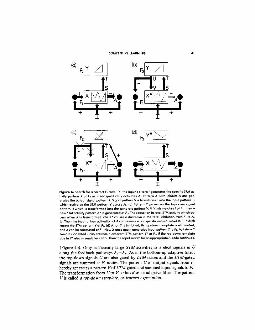
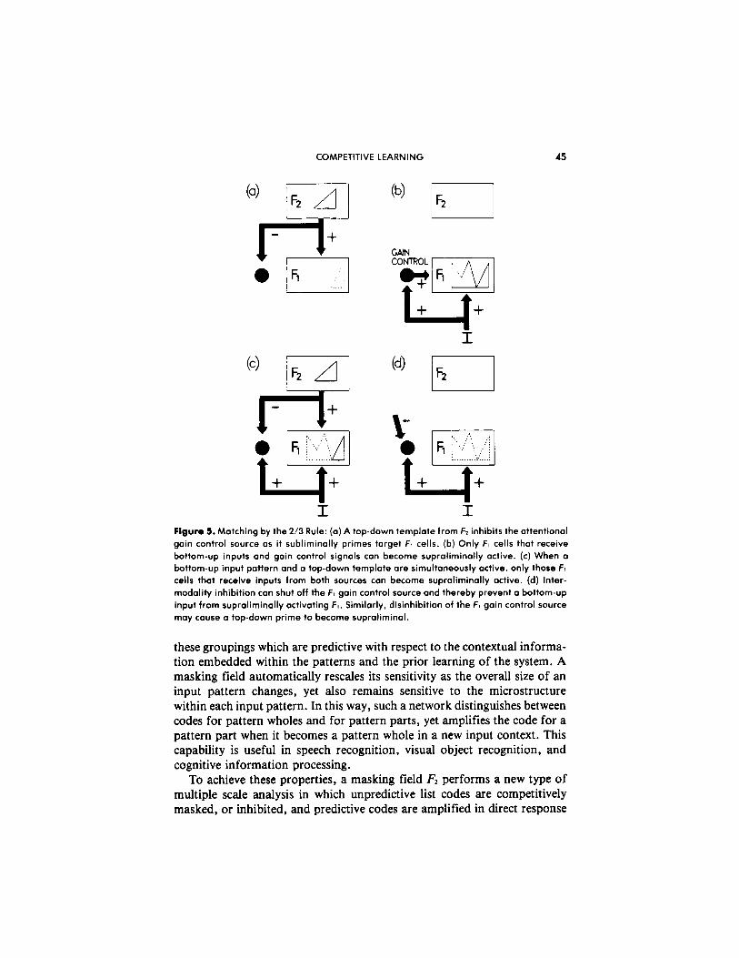
I Figure 5. Matching by the 2/3 Rule: (a) A top-down template from 15 inhibits the attentionol

gain control source as it subliminally primes target F, cells. (b) Only FI cells that receive

bottom-up inputs ond gain control signals con become supraliminally active. (c) When a

bottom-up input pattern and a top-down template are simultaneously active, only those FI

cells that receive inputs from both sources con become supraliminolly active. (d) Inter-

modality inhibition can shut off the F, gain control source and thereby prevent a bottom-up

input from supraliminolly activating F,. Similarly, disinhibition of the FI gain control source

may cause a top-down prime to become supraliminal.

these groupings which are predictive with respect to the contextual information embedded within the patterns and the prior learning of the system. A masking field automatically rescales its sensitivity as the overall size of an input pattern changes, yet also remains sensitive to the microstructure within each input pattern. In this way, such a network distinguishes between codes for pattern wholes and for pattern parts, yet amplifies the code for a pattern part when it becomes a pattern whole in a new input context. This capability is useful in speech recognition, visual object recognition, and cognitive information processing.

To achieve these properties, a masking field F2 performs a new type of multiple scale analysis in which unpredictive list codes are competitively masked, or inhibited, and predictive codes are amplified in direct response

0 a TOP-DOWN TEMPLATES (b) TOP-DOWN TEMPLATES 12345 12 3 4 5 6 7 8 9 10

2 = IR 3c PC p=.8 1 RES 4 D FF9

SE rE 1 RES

6 F LE

5 E FFDE 2 RES

6 F c,CDE

7~ rE 1 RES

7G FFD’ RES

8 H r ps 8H YCDEH 4 3 2 RES

9 I ly+x 9 I RES

FFD$H

10 J r 14 J RES

‘1 K r !BJ

12~ ra;,J

10 J FCDgsH

11 K FCDJk: RES

12 L F ksD J’:

'3 M c; I,.J M RES

14 N r l,.Jbl RES

13 M 7 l$Jk:M 1 RES

14 N F L 0 J b: kl RES

15 0 pJILI 15 0 F L W’ k: PI

‘6 P /-,I .Ji’I ‘6 P 7 L D ? b: i’l P 6 5 J 2 4 RES

n Q r 12. J I-I RES

18 R /=sI.J14

‘9 5 ly I T I4 . 2 RES

20T r I ,714 RES

'7 Q 5 lm~JK~lPGl 3 5 4 6 RES

‘8 R F L D I k: PI zsGl

‘9 5 7 $pTk:rlP5

4 2 RES

Figure 6. Alphabet leorning: Code learning in response to the first presentation of the first

20 letters of the olphobet is shown. Two different vigilonce levels were used, pz.5 and

p=.g. Each row represents the total code thot is learned ofier the letter at the left-hond

column of the row is presented at F,. Each column represents the critical feature pottern

that is learned through time by the F, node listed ot the top of the column. The critical

feoture patterns do not, in general, equal the pottern exemplars which change them through

learning. Instead, each critical feature pattern acts like a prototype for the entire set of

these exemplars, OS well OS for unfamiliar exemplars which shore invoriont properties with

fomilior exemplars. The simulation illustrates the “fast learning” case, in which the altered

LTM traces reach a new equilibrium in response to each new stimulus. Slow learning is

more groduol than this. (Reprinted with permission from Carpenter ond Grossberg, 1987b).

46


to trainable signals from an adaptive filter F, - F2 that is activated by an input source F, . An adaptive sharpening property obtains whereby a familiar input pattern causes a more focal spatial activation of its recognition code than an unfamiliar input pattern. The recognition code also becomes less distributed when an input pattern contains more information on which to base an unambiguous prediction of which input pattern is being processed. Thus, a masking field suggests a solution of the credit assignment problem by embodying a real-time code for the predictive evidence contained within its input patterns. Such a network processing level can be used to build up an ARTsystem F,-F,-F,-. . .with any number of processing levels.

16. THE BACK PROPAGATION AND NETtalk MODELS

The ARTarchitecture may be usefully compared with the back propagation (BP) model of Rumelhart, Hinton, and Williams (1986). The similarities and differences of these models highlight many of the types of formal comparisons that can help to evaluate other network learning models.

The BP model is a steepest descent algorithm in which each LTA4 trace, or weight, in the network is adjusted to minimize its contribution to the total mean square error between the desired and actual system outputs. Al- though steepest descent algorithms have a long history in technology and the neural modelling literature, the BP model has attracted widespread interest, partly because of the demonstration of Sejnowski and Rosenberg (1986), in which the BP algorithm is part of a system that learns to convert printed text into spoken language. Despite the appeal of this demonstration, the BP model does not model a brain process, as will be shown below. This shortcoming does not limit the model’s possible value in technological applications which can benefit from a steepest descent algorithm, but it under- mines the model’s usefulness in explaining behavioral or neural data.

The BP model is usually described as a three level model, with levels F, , F2, F,, such that level F2 is a level of “hidden units” between F, and F,. The purpose of the model is to learn an associative map between the input level F, and the output level F,. The map is designed to be sufficiently distributed to allow alterations in the inputs at F, to generate appropriate alterations in the outputs at F,. Such a possibility depends upon general projection properties of distributed associated maps (Kohonen, 1984). The key property demonstrated by computer simulations of the BPmodel is that it can learn a distributed associative map.

Some of the claims for the BP model have been based on comparisons with the early Perceptron model (Rosenblatt, 1962). Sejnowski and Rosen- feld (1986) have written that “until recently, learning in multilayered networks was an unsolved problem and considered by some impossible. . . In a multilayered machine the internal, or hidden, units can be used as feature detectors which perform a mapping between input units and output units,

48 GROSSBERG

and the difficult problem is to discover proper features.” Carpenter and Grossberg (1986) note, in contrast, that learning an associative map using hidden units is an old problem with definite solutions in the neural modelling literature subsequent to the introduction of the Perceptron. Indeed, ART was developed in part to develop a theory of how learning of an associative map could proceed in a self-stabilizing fashion (Figure 7). A basic difference does, however, exist between models of associative map learning, such as ART and the BP model. The former model is self-organizing, whereas the BP model requires an external teacher.

The way in which this teacher works is what distinguishes the BP model from other types of steepest descent learning algorithms, such as the classical Adaline model (Widrow, 1962). The teaching algorithm is also what makes the BP model impossible as a model of a brain process. In addition to the levels F,, F2, and F3 and the pathways F, - F2- F,, the BP model also requires levels F,, F,, F,, and F, as well as a complicated set of highly specific interactions between these levels and the rest of the network (Figure 8). These levels and interactions will now be described.

T PARALLEL PATTERN LEARNING

BOTTOM-UP CODE

LEARNING

TOP-DOWN EXPECTANCY LEARNING

Figure 7. Self-organization of an associative map can be accomplished using a network

with three levels 15, Fz, and FI. Levels F, and FZ regulate learning within bottom-up path-

ways FI-FZ and top-down pathways F,- FI. This learning process discovers compressed

recognition codes with invariant properties far the set of input patterns processed at F,. Ac-

tivation of these recognition codes at F, enables the activated sampling cells to learn output

patterns at F,. The total transformotion F, --b defines the associative mapping.

COMPETITIVE LEARNING

EXPECTED OUTPUTS

ISIGNALS I L 1 OUTPU’

SIGNALS 5

INPUTS I I 5

Figure 8. Circuit diagram of the bock propagation model: In addition to the processing

levels F,, f,, f,, there are also levels F., 15, F,, and h to carry out the computations which

control the learning process. The transport of learned weights from the F,--F, pathways to

the F. -F, pathways shows that this algorithm connot represent o learning process in the

brain.

Inputs delivered to F, propagate forward through F, to F,, where they generate the actual outputs of the network. The desired, or expected, outputs are independently delivered to level F, by an external teacher on every learning trial. The actual outputs are subtracted from the expected outputs at F, to generate error signals. These error signals propagate from F, to the F2- F, pathways, where they change the weights in the F,--F, pathways.

Back propagation proceeds as follows. The weights computed in the bottom-up F,- F, pathways are transported to the top-down F,- F5 pathways.

so GROSSBERG

Once in these pathways, the differences between expected and real outputs at F, are multiplied by the transported weights within the F,- F, pathways to generate weighted error signals that determine the inputs to F,. These inputs activate F,, which in turn generates output signals to the F, - F2 pathways. These output signals act as error signals which change the weights in the F, - F, pathways.

Such a physical transport of weights has no plausible physical interpreta- tion. The weights in the F,-F, pathways must be computed within these pathways in order to multiply signals from F2 to F,. These weights cannot also exist within the pathways from F, to F, in order to multiply signals from F, to F5 without being physically transported from (F2- F,) to (F4- F5) pathways, thereby violating basic properties of locality. Moreover, the levels F, and F, cannot be lumped together, because F, must record actual outputs, whereas F, must record differences between expected and actual outputs. The BP model is thus not a model of a brain process.

The computation of the error signal has an additional complexity. In addition to subtracting each actual output at F, from each expected output at F,, the derivative of each actual output is also computed. The difference between each expected and actual output is multiplied by the corresponding derivative in addition to being multiplied by the corresponding transported weight. Thus, there exist additional levels F6 and F, at each layer for con- verting outputs into derivatives of outputs before signalling these derivatives, with great positional specificity, to the correct transported weights (Figure 8). This complex interaction scheme must be replicated at every stage of hidden units that is used in a BP model.

17. COMPARING ADAPTIVE RESONANCE AND BACK PROPAGATION MODELS

Some BP mechanisms are evocative of ART mechanisms. The BP mechanisms do not, however, possess the key properties which endow an ART model with its computational power.

A. Stability The learned code of the BP model is unstable in a complex environment. It keeps tracking whatever expected outputs are imposed from outside. An omniscient teacher would be needed to decide if the model had learned enough in response to an unpredictable input environment. The learned code of an ART model is self-stabilizing in an arbitrary input environment.

B. Expectations as Exemplars or as Prototypes Within a BP model, an expected or template pattern is imposed on every trial by an external teacher. Errors are computed by comparing each component of the expected output pattern with the corresponding component of


the actual output pattern. There is no self-scaling property to alter the importance of each expected component when it is embedded in expected outputs of variable complexity. There is no concept of a critical feature pattern, or prototype. Instead, the expected pattern in a BPmodel is a particular exemplar at every stage of learning, rather than a prototype that gradually discovers invariant properties of all the exemplars that are ever experienced.

In contrast, an ARTmodel learns its own expectations without a teacher. Because an ARTmodel is self-scaling, it can learn critical feature patterns, or expected prototypes, by evaluating the predictive importance of particular features in input patterns of variable complexity at each stage of learning.

C. Weight Transport or Top-Down Template Learning In both a BP model and an ART model, both bottom-up and top-down LTM traces exist. In a BP model (Figure 8), the top-down LTM traces in F,- F5 pathways are formal transports of the learned F,-F, LTMtraces. In an ARTmodel (Figure l), the top-down LTMtraces in F,-F, pathways are directly learned by a real-time associative process. These top-down LTM weights are not transports of the learned LTMtraces in the F, - F2 pathways, and they need not equal these bottom-up LTMtraces. Thus, an ARTmodel is designed so that both bottom-up learning and top-down learning are part of a single information processing hierarchy, which can be realized by a locally computable real-time process.

D. Matching to Alter Information Processing and/or to Regulate Learning

In both the BP model and an ART model, there exists a concept of matching. Within an ART model, matching both alters information processing and regulates the learning process. In particular, the 2/3 Rule (Section 14) enables a top-down expectation to subliminally sensitize the network in preparation for any exemplar of an expected class of input patterns, and to coherently deform such an examplar, when it occurs, towards the prototype of the class. This STM transformation, also helps to regulate any learning that may be necessary to generate a globally self-consistent recognition code.

In contrast, matching within the BP model only changes LTM weights. It does not have any effects on the fast information processing that occurs within each input trial.

E. Learning an Associative Mapping BPand ARTprovide different descriptions of how associative maps between seen language and spoken language are learned. Figure 9 describes a macrocircuit that schematizes our conception of this process (Cohen & Grossberg, 1986; Grossberg, 1978, 1986, 1987b; Grossberg & Stone, 1986a). The associative map Vy- {A,, A,} in Figure 9 joins seen language to spoken language.

52 GROSSBERG

Unlike a BP model, all the learning of recognition codes that is triggered by auditory, visual, or motor patterns in Figure 9 is regulated by self-organizing mechanisms in reciprocal bottom-up and top-down adaptive filters. Once these codes self-stabilize their invariant recognition properties, the learning of associative maps between these code invariants can also proceed in a self- organizing fashion.

VISUAL OBJECT RECOGNITION SYSTEM

ITEM AND ORDER IN MOTOR STM

ICON IC MOTOR FEATURES

INPUTS ; GENERATED , AUDITORY

I FEEDBACK

Figure 9. A macrocircuit governing self-organization of recognition and recoil processes:

Auditorily mediated language processes (the AI). visual recognition processes (V’), and

motor control processes (the MI) interact internally via conditionable pathways (black lines)

and externally via environmental feedback (dotted lines) to self-organize the various pro-

cesses which occur at the different network stages.


F. Speech Invariants, Coherence, and Perception The NETtalk application of the back propagation algorithm (Sejnowski & Rosenberg, 1986) uses a familiar associative learning device: the number of nodes in F, and F, is chosen to be large enough to separate features of the inputs and outputs, thereby avoiding too much cross-talk in the associative map, but small enough to enable some generalization to occur among the distributed F, - F, projections. In particular, the time between letter scans is represented in NETtalk by leaving some coding slots in F, empty. This mechanism does not generalize to a model capable of computing the temporal in- variances of reading or speech perception.

The NETtalk model also makes the strong assumptions that exactly seven letter slots in F, correspond to a single, isolated phoneme slot in F,, and that this isolated phoneme slot corresponds to the entry in the middle letter slot. These assumptions prevent the model from attempting to solve the fundamental problem of how speech sounds are coherently grouped in real-time. Furthermore, it is not clear how a phoneme-by-phoneme match between actual output and expected output could be realized during a learning episode in vivo.

In addition to assuming the automatic isolation, scaling, and centering of information, NETtalk also postulates that each phoneme slot in F, contains 23 separate nodes. These nodes provide enough spatial dimensions to represent a large number of articulatory features, such as point of articulation, voicing, vowel height, etc. Extra nodes are introduced to encode stress and syllable boundaries. The model builds in the transformations from visual input to F, nodal representation and from F, nodal representation to phoneme sound. Because the model automates all of its F, and F, representations, all questions about visual and speech perception, as such, lie outside its scope.

The ARTspeech model in Figure 9 was derived from postulates concerning real-time constraints on speech learning and perception. In particular, the model includes mechanisms capable of learning some speech invariants (Grossberg, 1986, 1987b), and the top-down expectancies between its processing levels have coherent grouping properties. One of the primary function of such templates is to define and complete resonant contexts of features, no less than to generate error signals for self-regulating changes in associative weights.

In summary, the BP model suggests a new way to use steepest descent to learn associative maps between input and output environments which are statistically stationary and not too complex. Desirable properties of associative map learning are, however, shared by many associative learning models. Real-time network models must do more than learn an associative map or to store distributed codes for carefully controlled environments. Moreover, the use of an unphysical process such as weight transport in a model casts an un- answerable doubt over all empirical applications of the model.

54 GROSSBERG

18. CONCLUDING REMARKS

I conclude this essay with two general observations. The architectures of many popular learning and information processing models are often inadequate because they have not been constrained by the use of design principles whereby they could stably self-organize. Many models are actually incompatible with such constraints and some models utilize physically unrealiz- able formal mechanisms. Learning models which cannot adaptively cope with unpredictable changes in a complex environment have an unpromising future as models of mind and brain, and provide little hope of solving the outstanding cognitive problems which are not already well-handled by tra- ditional methods of artificial intelligence and engineering.

Models which do embody self-organization constraints in a fundamental way have frequently been shown to have a broader explanatory and predictive range than models which do not. Thus an analysis of learning, in particular of the mechanisms capable of self-stabilizing competitive learning, can lead psychology from metaphorical models to integrative theories which functionally and mechanistically express both a psychological and a neural reality.

APPENDIX 1

Competitive Learning Models Rumelhart and Zipser (1985, pp. 86-87) summarize competitive learning models as follows.

“1. The units in a given layer are broken into a set of nonoverlapping clusters. Each unit within a cluster inhibits every other unit within a cluster. The clusters are winner-take-all, such that the unit receiving the largest input achieves its maximum value while all other units in the cluster are pushed to the minimum value. We have arbitrarily set the maximum value to 1 and the minimum value to 0.

2. 3.

4.

5.

Every element in every cluster receives inputs from the same lines. A unit learns if and only if it wins the competition with other units in its cluster. A stimulus pattern Sj consists of a binary pattern in which each element of the pattern is either active or inactive. An active element is assigned the value 1 and an inactive element is assigned the value 0. Each unit has a fixed amount of weight (all weights are positive) which is distributed among its input lines. The weight on the line connecting unit i on the lower (or input) layer of unit j on the upper layer, is designated wi,. The fixed total amount of weight for unit j is designated Ciwi, = 1. A unit learns by shifting weight from its inactive to its active


input lines. If a unit does not respond to a particular pattern no leam- ing takes place in that unit. If a unit wins the competition, then each of its input lines gives up some proportion g of its weight and that weight is then distributed equally among the active input lines. More formally, the learning rule we have studied is:

Au,, = 0 if unit j loses on stimulus k

Gk (Al) gn,-g*, if unit j wins on stimulus k

where crl is equal to 1 if in stimulus pattern Sk unit i on the lower layer is active and zero otherwise, and n, is the number of active units in pattern S, (thus

n, = C c,J. ” I W)

Rumelhart and Zipser (1985, p. 87) go on to say that “This learning rule was proposed by Von der Malsburg (1973). As Grossberg (1976) points out, renormalization of the weights is not necessary.” Actually, this learning rule was proposed by Grossberg (1976a, 1976b), and is not the one used in the important article of Malsburg (1973), as I will show below.

A simple change of notation shows that the Rumelhart and Zipser (1985) model is identical with the Grossberg (1976a, 1976b) model. Equation (6) in Grossberg (1976b) is the learning equation

$a, = (- zi, +&)x*,,

for the long term memory (LTM) trace z,,. In (A3), xlj is the activity of the jth unit. Activity x, = 1 if unit j wins the competition and x2, = 0 if unit j loses the competition, as in equation (Al). In (A3),

4 ei =c,r, 644)

where 4 is the ith element of the input pattern. Function Bi in (A4) is the same as function ci,n,-’ in (Al) and (42). Function Bi is just the normalized input weight. The LTM trace zi, in (A3) is identical with the weight w,, in (Al). The factor g in (Al) just rescales the time variable, and thus adds no generality to the model.

By contrast, the learning rule used by Malsburg (1973) is (in my notation)

subject to the constraint

Ch = constant. (A61 m

56 GROSSBERG

Thus Malsburg (1973) normalized the LTM traces z,,,, which abut each unit j, not the input weights. The normalization constraint (A6) is, in fact, inconsistent with (AS) unless

CI, =o. (A71 m

Thus a rigorous application of Malsburg’s 1973 learning rule forces the choice of both positive and negative inputs, unlike the Grossberg (1976b) model that was used by Rumelhart and Zipser (1985). In his computer simulations, Malsburg implemented equations (AS) and (A6) in alternating time slices. The implication shown in (A7) is then not forced because neither (A5) nor (A6) is true at all times.

Malsburg (1973) needed condition (A6) because he simplified the learning law

d -jiZ” = -AZ,, + r,xzj (4

which was used in the competitive learning model of Grossberg (1972). In fact, the equations used by Malsburg (1973) are identical to the equations used by Grossberg (1972) with this one exception. As Malsburg (1973, p. 88) noted: “To answer these questions we have to write down the equations which govern the evolution of the system. They are summarized in Table 1 (compare Grossberg, 1972).” Term -Azij in (A8) describes the decay of LTM. Malsburg’s equation (AS) eliminates LTM decay. Since term &xzj is non-negative in these applications, the LTM trace in Malsburg’s equation (A5) can only increase. Without additional constraints, all LTM traces could therefore explode to infinity. Malsburg (1973) partially overcame this problem with his constraint (A6). The solution in equation (A3) was to pre- serve LTM decay (term - Az,) while normalizing the inputs I, to be learned. Then non-negative inputs Zi could freely be used, instead of inputs constrained by (A7).

Rumelhart and Zipser (1985) also mentioned and studied two related models. Equivalent models were introduced in Grossberg (1976b). These alternative models were designed to show that both of them also exhibit temporally unstable learning. Analysis of these variations of the simplest coding model confirmed that its unstable behavior was not an artifact of its simplicity.

Rumelhart and Zipser (1985) attributed one of these modified models to Bienenstock, Cooper, and Munro (1982). They noted that in such a model

a unit modulates its own sensitivity so that when it is not receiving enough inputs, it becomes increasingly sensitive. When it is receiving too many inputs, it decreases sensitivity. This mechanism can be implemented in the present context by assuming that there is a threshold and that the relevant activation is the degree to which the unit exceeds its threshold. If, whenever a unit fails to win it decreases its threshold, and whenever it does win it increases its threshold,


then this method will also make all of the units eventually respond, thereby engaging the mechanism of competitive learning (Rumelhart and Zipser, 1985, p. loo).

In equations (23)-(24) of Grossberg (1976b), such a variable-threshold model was introduced without changing the basic learning equation

643)

The sensitivity of x, to its inputs was modified as follows:

if S,(t)G,(r)> max{ S,(f)G,(f) : kfj} if S,(t)G,(t)c max{ &MC,(!) : k#j} 649)

where

G,U) =dl - f

fx21(V)K(f - v)dv), (AlO) 0

S,(t) is the total input to unit j, p(w) is an increasing function such that g(0) = 0 and g( 1) = 1, and K(w) is a decreasing function such that K(0) = 1 and K(m) =O; for example, K(w) =t?.

The history-dependent threshold is the term

f

t x2,( V)K(f - v)dv (All)

0

in equation (AlO). If unit j wins the competition then, by (A9), its activity x, becomes positive. Consequently, its threshold (Al 1) increases. If unit j loses the competition then, by (A9). its activity x, equals zero. Consequently, its threshold (Al 1) decreases. Thus, “a unit modulates its own sensitivity so that when it is not receiving enough inputs, it becomes increasingly sensitive.” By (A9) and (AlO), when a unit wins the competition, its activation level G,(t) “is the degree to which the unit exceeds its threshold.” Moreover, by (A3), the learning rate covaries with the activation G,(t) of unitj. Thus if unitj is active for a long time, then its threshold (Al 1) becomes large, so its learning rate (AlO) becomes small. The converse is also true: inactivity increases sensitivity and learning rate.

In the limiting case where the threshold in (Al 1) equals zero for all time because K= 0, this learning model reduces to the simplest competitive learning model. This can be seen as follows. If the threshold is set equal to zero, then G,(t)= 1 in (AlO). Hence, by (A9),

XZj(O = {

1 if S,(r)> max{ S, : kfj} 0 if S,(f)cmax{S, : kfj} ’ 6412)

In other words x2,(f) = 1 if unit j wins the competition, and x&) = 0 if unit j loses the competition, as in equation (Al).

58 GROSSBERG

Thus the model summarized by equations (A3), (A9), and (AlO) has all the properties described by Rumelhart and Zipser (1985) for a variable- threshold model and includes the simplest competitive learning model as a special case. In Grossberg (1976b, p. 132), it was noted that “Such a mechanism is inadequate if the training schedule allows v,[unit ~1 to recover its maximal strength.” I illustrated this inadequacy by displaying “an ordering of patterns that permits recoding of essentially all populations.”

Bienenstock, Cooper, and Munro (1982) studied a formally analogous model with a history-dependent threshold. However, they restricted their analysis to coding by a single unit j. Grossberg (1982c, p. 332), assumed the viewpoint of competitive learning and considered how that model behaves -in their coding application-when more than one coding unit j exists and the units compete with each other for activation. It was shown that persis- tent presentation of even a single unit pattern could cause temporally unstable coding in this competitive learning situation. This crippling form of instability seems to rule out the use of history-dependent thresholds as a viable learning rule, at least if the thresholds can recover from unit inactivity, which is the main property cited in their favor by Rumelhart and Zipser (1985, p. 100).

Rumelhart and Zipser (1985) call the third model variant that they study the leaky learning model. This model is a special case of the partial contrast model that was introduced in Grossberg (1976b, p. 132), where it was pointed out that, using such a model, “There can. . . be a shift in the locus of maximal responsiveness even to a single pattern-that is, recoding.” Rumelhart and Zipser (1985, p. 100) consider this a good property, rather than a bad one: “This change has the property that it slowly moves the losing units into the region where the actual stimuli lie, at which point they begin to capture some units and the ordinary dynamics of competitive learning take over.” These authors are willing to accept this instability property in order to avoid the even worse problem that “one of the units would have most of its weight on input lines that were never active, whereas another unit may have had most of its weight on lines common to all of the stimulus patterns. Since a unit never learns unless it wins, it is possible that one of the units will never win, and therefore never learn. This, of course, takes the competition out of competitive learning” (pp. 98-99).

This scheme cannot, however, be fully effective without having catas- trophic results on code stability. If the recoding is minor, then many nodes may remain unused and too many input patterns may be lumped together. In this case, the scheme cannot solve the problem for which it was introduced. Alternatively, major recoding may be allowed, but this property is just another way to describe a temporally unstable code.

The formal relationship between the leaky learning model and the partial contrast model is now summarized. In the leaky learning model, equation (Al) is replaced by


Awi, = Clk

8 Ti;-JwiJ if j loses on stimulus k Gk

& Ti;-g,wiJ if j wins on stimulus k (A131

where

g1=gw. (A141

In other words, slower learning occurs at losing units than at winning units. The leaky learning model is a variant of the partial contrast model. The partial contrast model continues to use the basic learning equation

$&J=(-&J+~,)-GJ, (A31

However, xzj is now defined by a partial contrast rule

&J = c Sm>.f(S) 0

(AW

wheref(w) is an increasing function of the total input S, to unitj, and 6 is a non-negative threshold. By (A15), the learning rate is fastest at the node x2, which receives the largest input Sj and is slower at other nodes, as in the leaky learning model. In summary, all of the types of models described by Rumelhart and Zipser (1985) were shown in Grossberg (1976b) to exhibit a basic problem of learning instability.

APPENDIX 2

Stable Code Learning for Sparse Input Patterns

To simplify notation, the simplest competitive learning model is defined again below: Let the input patterns Z,(f) across nodes vi in F, be immediately and perfectly normalized; that is, input 4(t) =O,Z(t) generates activity x,(t) = 8, at vi. The signals from a node vi in F, to nodes v, in F2 is chosen to be a linear function of the activity xi. For simplicity, let the signal emitted by v, equal Bi. The competition across nodes Vj in F, normalizes the total activity to the value 1 for definiteness and rapidly chooses that node v, for STM storage which receives the largest input; e.g., design F, as a cooperative- competitive feedback network with faster-than-linear or (properly chosen) sigmoid signal functions. These properties can be approximated by the simple rule that

‘= 1

1 if T,>max{e, T, : k#j}

0 if T,<max{e, T* : k#j}

where the total input TJ to v, is the inner product

T = p,zkJ.

(Al@

6417)

60 GROSSBERG

The L7’M traces in the F, - F2 pathways sample the pattern 8 = (0,) &, . . . ,&) of input signals only when their sampling cell is active. Thus.

$Z;j=fXj(-Zij+8,). (‘418)

This non-Hebbian associative law was introduced into the neural network literature in Grossberg (1969).

If a single pattern 0 is practiced, it maximizes the input q to its coding cell vj. Input T, increases as the classifying vector zj = (zij : iel) become parallel to 8 and the length 1 [zjl) of z, become normalized. Grossberg (1976b) also described circumstances under which a list of input patterns to F, could generate temporally stable learning capable of parsing these patterns into distinct recognition categories at F2. It was proved that, if not too many input patterns are presented, relative to the number of coding nodes in F,, or if the input patterns are grouped into not too many clusters, then the recognition code stabilizes and the classifying vectors approach the convex hull of the patterns which they code. The latter property shows that the classifying nodes ultimately receive maximal inputs consistent with the fact that the classifying vectors zj can fluctuate in response to all the input patterns that they code.

To state this theorem, the following notation is convenient. A partition e+>& of a finite set P is a subdivision of P into nonoverlapping and exhaus- tive subsets P,. The convex hull H(p) of P is the set of all convex combinations of elements of P. Given a set QC P, let R = P - Q denote the elements of P that are not in Q. The distance between a vector p and a set of vectors Q, denoted by 1 jp - QI I, is defined by I jp - QI I = inf() Ip - QI I : qE Q).

Suppose that, at time t, the classifying vector s(t) = (zij(t) : SE))) codes the set of patterns Pi(t); that is, node v, in F2 would be chosen if any pattern in P,(f) were presented at that time. Define P;(t) = P, (t) Uz,(t) and P*(f) = r/f=, Pi*(r).

Theorem (Stable Code Learning of Sparse Patterns) Let the network practice any finite set P = (V’) : I= 1,2,. . . , L) of input patterns. Suppose that at some time t = T, the partition e&P,(T) of P has the property that

min(u.v:uEP,(T),vEPj*(T))>max(u.v:uEP,(7),vEP*(T)-P:(7)) 6419)

for allj=l, 2,. . . ,J. Then the network partitions the patterns P into the stable categories P,(T); that is,

wo = p,(T) WO)

for allj= 1,2,. . . ,J and all tz T. In addition, learning maximizes the input to the classifying nodes; that is, the functions

4U) = I Iz,W - fm(O) I I (‘Ql)


are monotone decreasing for all j = 1, 2,. . . ,J and t L T. If, moreover, the patterns Pi( 7) are practiced in time intervals [U,, , Kk], k = 1,2,. . . , such that

6422)

then

lim II,(t) = 0. W3) I--

Thus the theorem describes circumstances under which practice of input patterns in P can cause the classifying vectors z,, which may have any initial distribution Z](O), to be separated well enough, as in (A19), to enable their later tuning to proceed, as in (A23), without disrupting the emergent partition CB&P,(~J of the patterns P into recognition categories.

REFERENCES

Banquet, J.-P., & Grossberg, S. (1987). Probing cognitive processes through the structure of event-related potentials during learning: An experimental and theoretical analysis. Applied Optics.

Bienenstock, E.L., Cooper, L.N., & Munro, P.W. (1982). Theory for the development of neuron selectivity: Orientation specificity and binocular interaction in visual cortex. Journal of Neuroscience, 2, 32-48.

Carpenter, G.A., & Grossberg, S. (1986). Associative learning, adaptive pattern recognition, and cooperative-competitive decision making by neural networks. In H. Szu (Ed.) Hybrid and Optical Computing. SPIE Proceedings.

Carpenter, G.A., & Grossberg, S. (1987a). Neural dynamics of category learning and recognition: Attention, memory consolidation, and amnesia. In J. Davis, R. Newburgh, & E. Wegman (Eds.), Brain structure, learning, and memory. AAAS Symposium Series.

Carpenter, G.A., & Grossberg, S. (1987b). A massively parallel architecture for a self-orga- nixing neural pattern recognition machine. Computer Vision, Graphics, and Image Processing, 37, 54-l 15.

Carpenter, G.A., & Grossberg, S. (1987~). Neural dynamics of category learning and recognition: Structural invariants, reinforcement, and evoked potentials. In M.L. Commons, S.M. Kosslyn, & R.J. Herrnstein (Eds.), Pattern recognition and concepts in animals, people, and machines.

Cohen, M.A., & Grossberg, S. (1986a). Neural dynamics of speech and language coding: De- velopmental programs, perceptual grouping, and competition for short term memory. Human Neurobiology, 5, 1-22.

Cohen, M.A., & Grossberg, S. (1987). Masking fields: A massively parallel neural architecture for learning, recognizing, and predicting multiple groupings of patterned data. Applied Optics.

Bstes, W.K. (1986). Memory storage and retrieval processes in category learning. Journal of Experimental Psychology: General, 115. 155-174.

Grossberg, S. (1969). On learning and energy-entropy dependence in recurrent and nonrecur- rent signed networks. Journal of Statistical Physics, 1, 319-350.

Grossberg, S. (1972). Neural expectation: Cerebellar and retinal analogs of cells fired by leam- able or unlearned pattern classes. Kybernetik, IO, 49-57.

Grossberg, S. (1975). A neural model of attention, reinforcement, and discrimination learning. International Review of Neurobiology, 18. 263-327.

62 GROSSBERG

Grossberg, S. (1976a). On the development of feature detectors in the visual cortex with applications to learning and reaction-diffusion systems. Biologicul Cybernetics, 21, 145-159.

Grossberg, S. (1976b). Adaptive pattern classification and universal recoding, I: Parallel development and coding of neural feature detectors. Biological Cybernetics, 23, 121-134.

Grossberg, S. (1976c). Adaptive pattern classification and universal recoding. II: Feedback, expectation, olfaction, and illusions. Biologicul Cybernetics, 23, 187-202.

Grossberg, S. (1978). A theory of human memory: Self-organization and performance of sen- sory-motor codes, maps, and plans. In R. Rosen & F. Snell (Eds.). Progress in theoreti- co/ biology, Vol. 5. (pp. 233-374). New York: Academic.

Grossberg, S. (1980). How does a brain build a cognitive code? Psychologicul Review, 87, 1-51.

Grossberg, S. (1982a). Studies of mind und bruin: Neurul principles of leurning, perception, development, cognition, and motor control. Boston: Reidel Press.

Grossberg, S. (1982b). Processing of expected and unexpected events during conditioning and attention: A psychophysiological theory. Psychological Review, 89, 529-572.

Grossberg, S. (1982c). Associative and competitive principles of learning and development: The temporal unfolding and stability of STM and LTM patterns. In S.I. Amari & M. Arbib (Eds.), Competition and cooperation in neural networks. New York: Springer- Verlag. Reprinted in Grossberg (1987a).

Grossberg, S. (1984). Unitization, automaticity, temporal order, and word recognition. Cogni- tion and Bruin Theory, 7, 263-283.

Grossberg, S. (1987c). The adaptive self-organization of serial order in behavior: Speech, language, and motor control. In E.C. Schwab & H.C. Nusbaum (Ms.), Puttern recognition by humuns und muchines, Vol. I: Speech perception. New York: Academic.

Grossberg. S. (1987a). The uduptive bruin, I: Cognition, leurning, reinforcement, and rhythm. Amsterdam: North-Holland.

Grossberg, S. (1987b). 7he uduptive bruin, II: Vision, speech, lunguuge, und motor control. Amsterdam: North-Holland.

Grossberg, S., & Gutowski, W. (1987). Neural dynamics of decision making under risk: Affec- tive balance and cognitive-emotional interactions. Psychologicul Review.

Grossberg, S., & Levine, D.S. (1987). Neural dynamics of attentionally modulated Pavlovian conditioning: Blocking, inter-stimulus interval, and secondary reinforcement. Sub- mitted for publication.

Grossberg, S., &Stone, G.O. (1986a). Neural dynamics of word recognition and recall: Atten- tional priming, learning, and resonance. Psychological Review, 93, 46-74.

Grossberg, S., & Stone, G.O. (1986b). Neural dynamics of attention switching and temporal order information in short-term memory. Memory und Cognition, 14, 451-468.

Hopfield, J.J. (1982). Neural networks and physical systems with emergent collective compu- tional abilities. Proceedings of the Nutionul Academy of Sciences, 79, 2554-2558.

Knapp, A.G., & Anderson, J.A. (1984). Theory of categorization based on distributed memory storage. Journul of Experimental Psychology: Leurning, Memory, and Cognition, 10, 616637.

Kohonen, T. (1984). Self-organization and ussociutive memory. New York: Springer-Verlag. Malsburg, C. von der (1973). Self-organization of orientation sensitive cells in the striate cor-

tex. Kybernetik, 14, 85-100. McClelland, J.L. (1985). Putting knowledge in its place: A scheme for programming parallel

processing structures on the fly. Cognitive Science, 9. 113-146. McClelland, J.L., & Rumelhart, D.E. (1981). An interactive activation model of context ef-

fects in letter perception, Part 1: An account of basic findings. Psychologicul Review, 88, 375-407.

McClelland, J.L., & Rumelhart, D.E. (1985). Distributed memory and the representation of general and specific information. Journul of Experimental Psychology: Generul, 114. 159-188.


Posner. M.I. (1973). Cognifion: An introducfion. Glenview, IL: Scott, Foresman. and Co. Posner, M.I., & Keele, S.W. (1968). On the genesis of abstract ideas. Journalof Experimental

Psychology, 77, 353-363. Posner, M.I., & Keele, SW. (1970). Retention of abstract ideas. Journal of Experimental

Psychology, 83, 304-308. Rosenblatt. F. (1962). Principles of neurodynamics. Washington, DC: Spartan. Rumelhart, D.E., Hinton, G.E., &Williams, R.J. (1985, September). Learning internal repre-

sentations by error propagation. Institutefor Cognitive Science Report 8506, University of California at San Diego.

Rumelhart, D.E., & McClelland, J.L. (1982). An interactive model of context effects in letter perception, Part 2: The contextual enhancement effect and some tests and extensions of the model. Psychological Review, 89, 60-94.

Rumelhart, D.E., & Zipser, D. (1985). Feature discovery by competitive learning. Cognitive Science, 9, 75- 112.

Salasoo, A., Shiffrin, R.M., & Feustal, T.C. (1985). Building permanent memory codes: Codi-

fication and repetition effects in word identification. Journal of Expermental Psychol- ogy: General, 114, 50-77.

Samuel, A.G., van Santen, J.P.H., & Johnston, J.C. (1982). Length effects in word perception: We is better than I but worse than you or them. Journal of Experimental Psychol- ogy: Human Perception and Performance, 8. 91-105.

Samuel, A.G., van Santen, J.P.H., & Johnston, J.C. (1983). Reply to Matthei: We really is worse than you or them, and so are ma and pa. Journal of Experimental Psychology: Human Perception and Performance, 9, 321-322.

Sejnowski, T.J., & Rosenberg, CR. (1986, January). NETtalk: A parallel-network that learns to read aloud. Johns Hopkins University.

Wheeler, D.D. (1970). Processes in word recognition. Cognitive Psychology, I, 59-85. Widrow, B. (1962). Generalization and information storage in networks of Adaline neurons.

In M.C. Yovits, G.T. Jacobi, & G.D. Goldstein (Eds.), Self-organizing systems. Wash- ington, DC: Spartan.

competitive learning: from interactive activation to...

Documents