2017 Enterprise Risk Management Symposium

April 20–21, 2017, New Orleans

Competitive Premium Pricing and Cost Savings for Insurance Policyholders: Leveraging Big Data

By Ivelin M. Zvezdov and Sebastian Rath

Copyright © 2017 by the Society of Actuaries, Casualty Actuarial Society, and the Canadian Institute of Actuaries. All rights reserved by the Society of Actuaries, Casualty Actuarial Society, and the Canadian Institute of Actuaries. Permission is granted to make brief excerpts for a published review. Permission is also granted to make limited numbers of copies of items in this monograph for personal, internal, classroom or other instructional use, on condition that the foregoing copyright notice is used so as to give reasonable notice of the Society of Actuaries’, Casualty Actuarial Society’s, and the Canadian Institute of Actuaries’ copyright. This consent for free limited copying without prior consent of the Society of Actuaries, Casualty Actuarial Society, and the Canadian Institute of Actuaries does not extend to making copies for general distribution, for advertising or promotional purposes, for inclusion in new collective works or for resale. The opinions expressed and conclusions reached by the authors are their own and do not represent any official position or opinion of the Society of Actuaries, Casualty Actuarial Society, or the Canadian Institute of Actuaries or their members. The organizations make no representation or warranty to the accuracy of the information.

1

Competitive Premium Pricing and Cost Savings for Insurance Policyholders: Leveraging Big Data

Ivelin M. Zvezdov, M.Phil.1

Sebastian Rath, Ph.D.2

Abstract

This paper’s purpose is to examine the intersection of research on the effects of insurance risk diversification and availability of big insurance data components for competitive underwriting and premium pricing. We study the combination of physical diversification by geography and insured natural peril with the complexity of aggregate structured insurance products, and how big historical and modeled data components impact product underwriting decisions. Under such market conditions, the availability of big data components facilitates accurate measurement of interdependencies among risks, as well as the definition of optimal and competitive insurance premium at the level of the firm and the policyholders. We extend the discourse to a notional microeconomy and examine the impact of diversification and insurance big data components on the potential for developing strategies for sustainable and economical insurance policy underwriting. We review concepts of parallel and distributed algorithmic computing for big data clustering, mapping and resource-reducing algorithms.

Introduction

This working paper will examine how big data and fast compute platforms solve some complex premium-pricing, portfolio-structuring and accumulation problems in the context of flood insurance markets. Our second objective is to measure the effects of geospatial insurance risk diversification through modeling of interdependencies and show that such measures impact single risk premium definition and its market cost. The single product case studies examine the pricing of insurance umbrella coverage. They are selected to address scenarios relevant to current insurance market conditions under intense premium competition. We extend the discourse to a microeconomy of multiple policyholders and aim to generalize some findings on economies of scale and diversification. The outcomes of all case studies and theoretical analysis depend on the

1 Ivelin M. Zvezdov is senior product manager at AIR Worldwide, VERISK Analytics Corp., in Boston. He can be reached at izvezdov@air-worldwide.com or ivelin.zvezdov@gmail.com. 2 Sebastian Rath is principal insurance risk officer at NN Group, Rotterdam, The Netherlands. He can be reached at Sebastian.Rath@gmail.com.

2

availability of big insurance data components for modeling and pricing workflows. The quality, usability and computational cost of such data components determine their direct impact on the underwriting and pricing process and on definition of the single risk cost of insurance.

1.0 Pricing Aggregate Umbrella Policies

Insurers are competing actively for insureds’ premiums and looking for economies of scale to offset and balance premium competition and thus develop more sustainable long-term underwriting strategies. While writing competitive premium policies and setting up flexible contract structures, insurers are mindful of risk concentration and the lower bounds of fair technical pricing. Structuring of aggregate umbrella policies lends itself to underwriting practices of larger scales in market share and diversification. Only large insurers have the economies of scale to offer such products to their clients.

Premium pricing of umbrella and global policies relies on both market conditions and a mathematical modeling argument. On the market and operational side, the insurer relies on the lower cost of umbrella products due to efficiencies of scale in brokerage, claims management, administration and, even, in the computational scale-up of the modeling and pricing internal functions of its actuarial departments. In our study, we will first focus on the statistical modeling argument, then we will define big data components, which allow for solving such policy structuring and pricing problem.

We first set up the case study on a smaller scale in context of two risks—with insured limits for flood of 90 million and 110 million respectively. These risks are priced for combined river/rain and storm surge flood coverage, first with both single limits separately and independently and then in an aggregate umbrella insurance product with a combined limit of 200 million, as seen in Equation (1.0) and Table 1.

𝑈𝑈𝑈𝑈𝑈𝑈𝑈𝑈𝑈𝑈𝑈𝑈𝑈𝑈𝑈𝑈 (200𝑀𝑀) = 𝐿𝐿𝐿𝐿𝑈𝑈𝐿𝐿𝐿𝐿 1 (90𝑀𝑀) + 𝐿𝐿𝐿𝐿𝑈𝑈𝐿𝐿𝐿𝐿 2 (110𝑀𝑀). (1.0)

Table 1. Policy Setup and Limit Coverage Policy Setup Limit Coverage

Policy 1, π(S) 90M

Policy 2, π(Q) 110M

Umbrella, π(S + Q) 200M

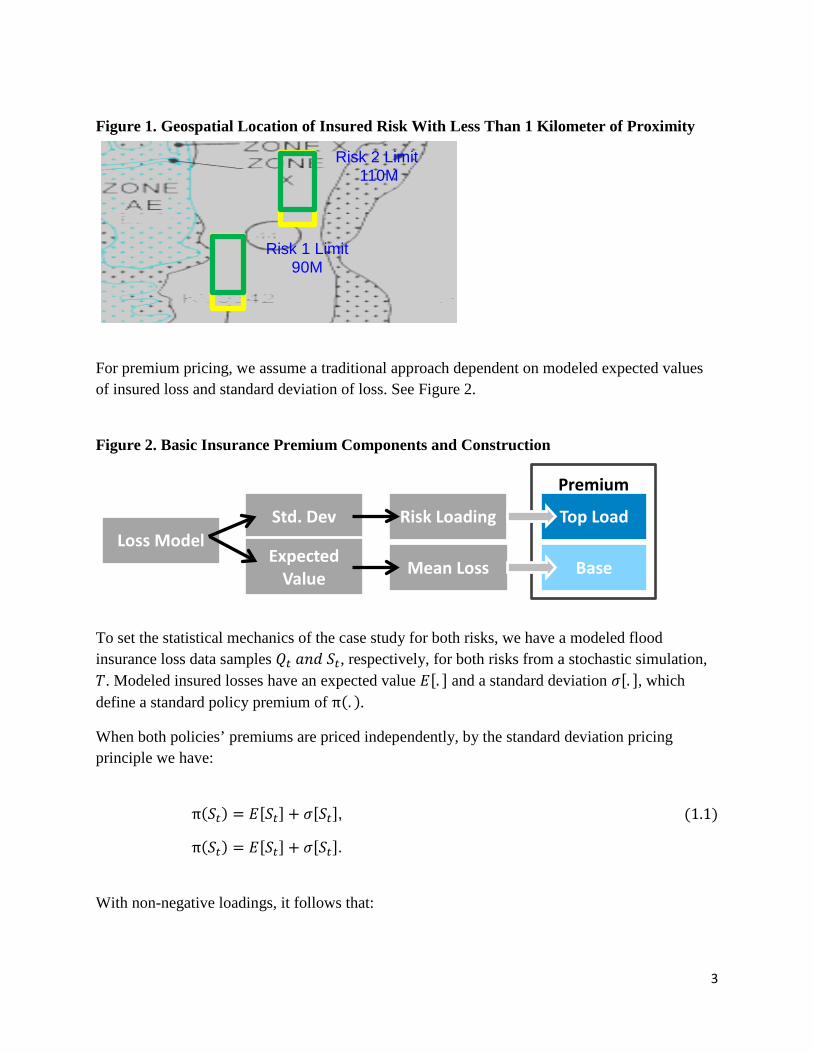
The two risks are owned by a single insured and are located in a historical flood zone, in geospatial proximity to each other, of less than 1 kilometer, as seen in Figure 1.

3

Figure 1. Geospatial Location of Insured Risk With Less Than 1 Kilometer of Proximity

For premium pricing, we assume a traditional approach dependent on modeled expected values of insured loss and standard deviation of loss. See Figure 2.

Figure 2. Basic Insurance Premium Components and Construction

To set the statistical mechanics of the case study for both risks, we have a modeled flood insurance loss data samples 𝑄𝑄𝑡𝑡 𝑈𝑈𝑎𝑎𝑎𝑎 𝑆𝑆𝑡𝑡, respectively, for both risks from a stochastic simulation, 𝑇𝑇. Modeled insured losses have an expected value 𝐸𝐸[. ] and a standard deviation 𝜎𝜎[. ], which define a standard policy premium of π(. ).

When both policies’ premiums are priced independently, by the standard deviation pricing principle we have:

π(𝑆𝑆𝑡𝑡) = 𝐸𝐸[𝑆𝑆𝑡𝑡] + 𝜎𝜎[𝑆𝑆𝑡𝑡],

π(𝑆𝑆𝑡𝑡) = 𝐸𝐸[𝑆𝑆𝑡𝑡] + 𝜎𝜎[𝑆𝑆𝑡𝑡].

(1.1)

With non-negative loadings, it follows that:

Risk 1 Limit 90M

Risk 2 Limit 110M

Loss Model Risk Loading Std. Dev

Expected Value

Mean Loss Base

Premium

Top Load

4

π(𝑆𝑆𝑡𝑡) ≧ 𝐸𝐸[𝑆𝑆𝑡𝑡],

π(𝑄𝑄𝑡𝑡) ≧ 𝐸𝐸[𝑄𝑄𝑡𝑡].

(2.0)

Since both risks are owned by the same insured, we aggregate the two standard premium equations, using traditional statistical accumulation principles for expected values and standard deviations of loss:

π(𝑄𝑄𝑡𝑡) + π(𝑆𝑆𝑡𝑡) = 𝐸𝐸[𝑆𝑆𝑡𝑡] + 𝜎𝜎[𝑆𝑆𝑡𝑡] + 𝐸𝐸[𝑄𝑄𝑡𝑡] + 𝜎𝜎[𝑄𝑄𝑡𝑡],

π(𝑄𝑄𝑡𝑡) + π(𝑆𝑆𝑡𝑡) = 𝐸𝐸[𝑆𝑆𝑡𝑡 + 𝑄𝑄𝑡𝑡] + 𝜎𝜎[𝑆𝑆𝑡𝑡] + 𝜎𝜎[𝑄𝑄𝑡𝑡].

(3.0)

The theoretical joint insured loss distribution function 𝑓𝑓𝑆𝑆,𝑄𝑄(𝑆𝑆𝑡𝑡,𝑄𝑄𝑡𝑡) of the two risks will have an expected value of insured loss:

𝐸𝐸[𝑆𝑆𝑡𝑡 + 𝑄𝑄𝑡𝑡] = 𝐸𝐸[𝑆𝑆𝑡𝑡] + 𝐸𝐸[𝑄𝑄𝑡𝑡], (4.0)

and a joint theoretical standard deviation of insured loss:

𝜎𝜎[𝑆𝑆𝑡𝑡 + 𝑄𝑄𝑡𝑡] = �𝜎𝜎2[𝑆𝑆𝑡𝑡] + 𝜎𝜎2[𝑄𝑄𝑡𝑡] + 2𝜌𝜌𝜎𝜎[𝑆𝑆𝑡𝑡]𝜎𝜎[𝑄𝑄𝑡𝑡]. (4.1)

We use further these aggregation principles to express the sum of two single risks premiums, π(𝑄𝑄𝑡𝑡),π(𝑆𝑆𝑡𝑡), as well as to derive a combined premium π(𝑄𝑄𝑡𝑡 + 𝑆𝑆𝑡𝑡) for an umbrella coverage product insuring both risks with equivalency in limits as in Equation (1.0). An expectation for full equivalency in premium definition produces the following equality:

π(𝑄𝑄𝑡𝑡 + 𝑆𝑆𝑡𝑡) = 𝐸𝐸[𝑆𝑆𝑡𝑡 + 𝑄𝑄𝑡𝑡] + �𝜎𝜎2[𝑆𝑆𝑡𝑡] + 𝜎𝜎2[𝑄𝑄𝑡𝑡] + 2𝜌𝜌𝜎𝜎[𝑆𝑆𝑡𝑡]𝜎𝜎[𝑄𝑄𝑡𝑡]

= π(𝑄𝑄𝑡𝑡) + π(𝑆𝑆𝑡𝑡).

(4.2)

The expression introduces a correlation factor 𝜌𝜌 between modeled insured losses of the two policies. In our case study, this correlation factor specifically expresses dependencies between historical and modeled losses for the same insured peril due to geospatial distances. Such correlation factors are derived by algorithms that measure dependencies of historical and modeled losses on their sensitivities to geospatial distances among risks. In this article, we will not delve into the definition of such geospatial correlation algorithms. Three general cases of

5

dependence relationships among flood risks due to their geographical situation and distances are examined in our article: full independence, full dependence and partial dependence.

2.0 Subadditivity, Dependence and Diversification

2.1 Two Boundary Cases of Fully Dependent and Fully Independent Risks

In the first boundary case, where we study full dependence between risks, expressed with a unit correlation factor, we have from first statistical principles that the theoretical sum of the standard deviations of loss of the fully dependent risks is equivalent to the standard deviation of the joint loss distribution of the two risks combined, as defined in Equation (4.1).

𝜎𝜎[𝑆𝑆𝑡𝑡 + 𝑄𝑄𝑡𝑡] = �𝜎𝜎2[𝑆𝑆𝑡𝑡] + 𝜎𝜎2[𝑄𝑄𝑡𝑡] + 2𝜎𝜎[𝑆𝑆𝑡𝑡]𝜎𝜎[𝑄𝑄𝑡𝑡] = 𝜎𝜎[𝑆𝑆𝑡𝑡] + 𝜎𝜎[𝑄𝑄𝑡𝑡]. (4.3)

For expected values of loss, we already have a known theoretical relationship between single risks’ expected insurance loss and umbrella product expected loss in Equation (4.0). The logic of summations and equalities for the two components in standard premium definition in equations (4.0) and (4.3) leads to deriving a relationship of proven full additivity in premiums between the single policies and the aggregate umbrella product, as seen in Equation (4.2), and shortened as:

π(𝑄𝑄𝑡𝑡 + 𝑆𝑆𝑡𝑡) = π(𝑄𝑄𝑡𝑡) + π(𝑆𝑆𝑡𝑡). (4.4)

Some underwriting conclusions are evident. When structuring a combined umbrella product for fully dependent risks, in very close to identical geographical space, same insured peril and line of business, the price of the aggregated umbrella product should approach the sum of single risk premiums priced independently. The absence of diversification in geography and insured catastrophe peril prevents any significant opportunities for cost savings or competitiveness in premium pricing. The summation of riskiness form single policies to aggregate forms of products is linear and co-monotonic. Economies of market share scale do not play a role in highly clustered and concentrated pools of risks, where diversification is not achievable and interrisk dependencies are close to perfect. In such scenarios, the impact of big data components to underwriting and pricing practices is not as prominent because formulation of standard premiums for single risks and aggregated products could be achieved by theoretical formulations.

In our second boundary case of full and perfect independence, when two or more risks with two separate insurance limits are priced independently and separately, the summation of their premiums is still required for portfolio accumulations by line of business and geographic and administrative region. This premium accumulation task or “roll-up” of fully independent risks is

6

accomplished by practitioners accordingly with the linear principles of Equation (3.0). However, if we are to structure an aggregate umbrella cover for these same single risks with an aggregated premium of π(𝑄𝑄𝑡𝑡 + 𝑆𝑆𝑡𝑡) , the effect of statistical independence expressed with a zero correlation factor will reduce Equation (3.0) to Equation (5.0):

π(𝑄𝑄𝑡𝑡 + 𝑆𝑆𝑡𝑡) = 𝐸𝐸[𝑆𝑆𝑡𝑡 + 𝑄𝑄𝑡𝑡] + �𝜎𝜎2[𝑆𝑆𝑡𝑡] + 𝜎𝜎2[𝑄𝑄𝑡𝑡]. (5.0)

Full independence among risks more strongly than any other case supports the premium subadditivity principle, which is stated in Equation (6.0).

π(𝑄𝑄𝑡𝑡 + 𝑆𝑆𝑡𝑡) ≦ π(𝑄𝑄𝑡𝑡) + π(𝑆𝑆𝑡𝑡). (6.0)

An expanded expression of the subadditivity principle is easily derived from the linear summation of premiums in Equation (3.0) and the expression of the combined single insurance product premium in Equation (5.0).

Some policy and premium underwriting guidelines can be derived from this regime of full statistical independence. Under conditions of full independence, when two risks are priced independently and separately, the sum of their premiums will always be larger than the premium of an aggregate umbrella product covering these same two risks. The physical and geographic characteristics of full statistical independence for modeled insurance loss are large geospatial distances and independent insured catastrophe perils and business lines. In practice, this is generally defined as insurance risk portfolio diversification by geography, line and peril. In insurance product terms, we proved that diversification by geography, peril and line of business, which are the physical prerequisites for statistical independence, allow structuring and pricing an aggregate umbrella product with a premium less than the sum of the independently priced premiums of the underlying insurance risks.

In this case, unlike with the case of full dependence, big data components have a computing and accuracy function to play in the underwriting and price-definition process. Once the subadditivity of the aggregate umbrella product premium as in Equation (6.0) is established, the premium is back-allocated to the single component risks covered by the insurance product. This is done to measure the relative riskiness of the assets under the aggregate insurance coverage and each risk’s individual contribution to the formation of the aggregate premium. Back-allocation is described further in the article in the context of a notional microeconomy case.

7

2.2 Less Than Fully Dependent Risks Scenario

In our case study, we have geospatial proximity of the two insured risks in a known flood zone with measured and available averaged historical flood intensities, which leads to a measurable statistical dependence of modeled insurance loss. We express this dependence with a computed correlation factor in the interval [0 < 𝜌𝜌′ < 1.0].

Partial dependence with a correlation factor 0 < 𝜌𝜌′ < 1.0 has immediate impact on the theoretical standard deviation of combined modeled loss, which is a basic quantity in the formulation of risk and loading factors for premium definition.

𝜎𝜎[𝑆𝑆𝑡𝑡 + 𝑄𝑄𝑡𝑡] = �𝜎𝜎2[𝑆𝑆𝑡𝑡] + 𝜎𝜎2[𝑄𝑄𝑡𝑡] + 2𝜌𝜌′𝜎𝜎[𝑆𝑆𝑡𝑡]𝜎𝜎[𝑄𝑄𝑡𝑡] ≦ 𝜎𝜎[𝑆𝑆𝑡𝑡] + 𝜎𝜎[𝑄𝑄𝑡𝑡]. (6.5)

This leads to redefining the equality in Equation (4.3) to an expression of inequality between the premium of the aggregate umbrella product and the independent sum of the single risk premiums, as in the case of complete independence.

π(𝑄𝑄𝑡𝑡 + 𝑆𝑆𝑡𝑡) = 𝐸𝐸[𝑆𝑆𝑡𝑡 + 𝑄𝑄𝑡𝑡] + �𝜎𝜎2[𝑆𝑆𝑡𝑡] + 𝜎𝜎2[𝑄𝑄𝑡𝑡] + 2𝜌𝜌′𝜎𝜎[𝑆𝑆𝑡𝑡]𝜎𝜎[𝑄𝑄𝑡𝑡]

≦ π(𝑄𝑄𝑡𝑡) + π(𝑆𝑆𝑡𝑡).

(7.0)

The principle of premium subadditivity, Equation (6.0), as in the case of full independence, again comes into force. The expression of this principle is not as strong with partial dependence as with full statistical independence, but we can clearly observe a theoretical ranking of aggregate umbrella premiums π(𝑄𝑄𝑡𝑡 + 𝑆𝑆𝑡𝑡) in the three cases reviewed so far:

π 𝐹𝐹𝐹𝐹𝐹𝐹𝐹𝐹 𝐼𝐼𝐼𝐼𝐼𝐼𝐼𝐼𝐼𝐼𝐼𝐼𝐼𝐼𝐼𝐼𝐼𝐼𝐼𝐼𝐼𝐼𝐼𝐼 ≦ π 𝑃𝑃𝑃𝑃𝑃𝑃𝑡𝑡𝑃𝑃𝑃𝑃𝐹𝐹 𝐷𝐷𝐼𝐼𝐼𝐼𝐼𝐼𝐼𝐼𝐼𝐼𝐼𝐼𝐼𝐼𝐼𝐼𝐼𝐼 ≦ π 𝐹𝐹𝐹𝐹𝐹𝐹𝐹𝐹 𝐷𝐷𝐼𝐼𝐼𝐼𝐼𝐼𝐼𝐼𝐼𝐼𝐼𝐼𝐼𝐼𝐼𝐼𝐼𝐼. (7.1)

This theoretical ranking is further confirmed in the next section with computed numerical results.

Less than full dependencies (i.e., partial dependencies among risks) could still be viewed as a statistical modeling argument for diversification in market share geography, line of business and insured peril. Partial but effective diversification still offers an opportunity for competitive premium pricing. In insurance product and portfolio terms, our study proves that partial or imperfect diversification by geography affects the sensitivity of premium accumulation and allows for cost savings in premium for aggregate umbrella products vs. the summation of multiple single risk policy premiums.

8

3.0 Numerical Results of Single Risk and Aggregate Premium Pricing Cases

In our flood risk premium study, we modeled and priced three scenarios, using classical formulas for a single risk premium in Equation (1.0) and for umbrella policies in Equation (7.0). In our first scenario, we price each risk separately and independently with insured limits of 90 million and 110 million. In the second and third scenarios, we price an umbrella product with a limit of 200 million, in three subcases with {1.0, 0.3 𝑈𝑈𝑎𝑎𝑎𝑎 0.0} correlation factors, respectively, to represent full dependence, partial dependence and full independence of modeled insured loss. We use stochastic modeled insurance flood losses computed with high geospatial granularity of 30 meters. See Table 2.

Table 2. Numerical Results of Premium Pricing Under Three Dependence Structures

Insured Limit(s) Policy & Premium Set Up Premium Dependence & Additivity 90M Policy 1: π(1) 512K

110M Policy 2: π(2) 725K

200M Premium sum: π(1) + π(2) 1.24M Full dependence & additivity 200M Umbrella: π(1 + 2):

100% correlation 1.24M Full dependence & additivity

200M Umbrella: π(1 + 2): 30% correlation

1.02M Partial dependence & subadditivity

200M Umbrella: π(1 + 2): 0% correlation

0.9M Full independence & subadditivity

The numerical results of our experiment fully support the conclusions and guidelines we earlier derived from theoretical statistical relationships. For fully dependent risks in close proximity, the sum of single risk premiums approaches the price of an umbrella product, which is priced with 1.0 (100%) correlation factor. This is the stochastic relationship of full premium additivity. For partially dependent risks, the price of a combined product, modeled and priced with a 0.3 (30%) correlation factor, could be less than the sum of single risk premiums. For fully independent risks, priced with a 0 (0.0%) correlation factor, the price of the combined insurance cover will further decrease to the price of an umbrella on partially dependent risks (30% correlation). Partial dependence and full independence support the stochastic ordering principle of premium subadditivity. The premium ranking relationship in Equation (7.1) is strongly confirmed by these numerical pricing results.

Less than full dependence among risks, which is a very likely and practical measurement in real insurance umbrella coverage products, could still be viewed as the statistical modeling argument for diversification in market share geography. Partial and incomplete dependence theoretically

9

and numerically supports the argument that partial but effective diversification offers an opportunity for competitive premium pricing.

4.0 Theoretical Expansion to a Single Firm Microeconomy Case

We expand the discourse to a simple theoretical microeconomy and examine if the same principles derived for the aggregate umbrella insurance product still hold on the larger scale of an insurance firm. In a notional economy with {1 … 𝐿𝐿𝑡𝑡…𝑁𝑁} insurance risks 𝑈𝑈1,𝑁𝑁 and policyholders respectively, we have only one insurance firm, which at time 𝑇𝑇 does not have an information data set 𝜃𝜃𝑇𝑇 about dependencies among per-risk losses. Each premium is estimated by the traditional standard deviation principle in Equation (1.1). For the same time period 𝑇𝑇, the insurance firm collects a total premium 𝜋𝜋𝑇𝑇[𝐿𝐿𝑡𝑡𝐿𝐿𝑈𝑈𝑈𝑈] equal to the linear sum of all {1 … 𝐿𝐿𝑡𝑡…𝑁𝑁} policy premiums 𝜋𝜋𝑇𝑇[𝑈𝑈𝑁𝑁] in the notional economy:

𝜋𝜋𝑇𝑇[𝑈𝑈1] + … + 𝜋𝜋𝑇𝑇[𝑈𝑈𝑁𝑁] = ∑ 𝜋𝜋𝑇𝑇𝑁𝑁

𝑃𝑃=1 = 𝜋𝜋𝑇𝑇[𝐿𝐿𝑡𝑡𝐿𝐿𝑈𝑈𝑈𝑈]. (8.0)

There is full additivity in portfolio premiums, and, because of unavailability of data on interrisk dependencies for modeling, the insurance firm cannot take advantage of competitive premium cost savings due to market share scale and geographical distribution and diversification of the risks in its book of business. For coherence, we assume all insurance risks and policies belong to the same line of business and cover the same insured natural peril—flood—so that the only insurance risks diversification possible is due to insurance risk independence derived from geospatial distances. A full premium additivity equation similar to an aggregate umbrella product premium seen in Equation (3.0), extended for the case of the total premium of the insurance firm in our microeconomy, is composed in Equation (9.0):

𝜋𝜋𝑇𝑇[𝐿𝐿𝑡𝑡𝐿𝐿𝑈𝑈𝑈𝑈] = 𝜋𝜋𝑇𝑇[𝑈𝑈1] + … + 𝜋𝜋𝑇𝑇[𝑈𝑈𝑁𝑁] = 𝐸𝐸[𝑈𝑈1 + ⋯+ 𝑈𝑈𝑁𝑁] + 𝜎𝜎[𝑈𝑈1] + ⋯+ 𝜎𝜎[𝑈𝑈𝑁𝑁]. (9.0)

In the next time period 𝑇𝑇 + 1, the insurance firm acquires a data set 𝜃𝜃𝑇𝑇+1, which allows it to model geospatial dependencies among risks and to identify fully dependent, partially dependent and fully independent risks. The dependence structure is expressed and summarized in a [𝑁𝑁 𝑥𝑥 𝑁𝑁] correlation matrix: 𝜌𝜌𝑃𝑃,𝑁𝑁. Traditionally, full independence between any two risks is modeled with a zero correlation factor, and partial dependence is modeled by a correlation factor less than one. With this new information, we can extend the insurance product expression in Equation (7.0) to the total accumulated premium 𝜋𝜋𝑇𝑇+1[𝐿𝐿𝑡𝑡𝐿𝐿𝑈𝑈𝑈𝑈] of the insurance firm at time 𝑇𝑇 + 1:

10

∑ 𝜋𝜋𝑇𝑇+1𝑁𝑁𝑃𝑃=1 = 𝐸𝐸[𝑈𝑈1 + ⋯+ 𝑈𝑈𝑁𝑁] + �∑ 𝜎𝜎2[𝑈𝑈𝑃𝑃]1,𝑁𝑁 + ∑ 2𝜌𝜌𝑃𝑃,𝑁𝑁𝜎𝜎[𝑈𝑈𝑃𝑃]𝜎𝜎[𝑈𝑈𝑁𝑁]1,𝑁𝑁 . (10.0)

The impacts of full independence and partial dependence, which are inevitably present in a full insurance book of business, guarantee that the subadditivity principle for premium accumulation comes into effect. In our case study, subadditivity has two related expressions. Between the two time periods, the acquisition of the dependence data set 𝜃𝜃𝑇𝑇, which is used for modeling and definition of the correlation structure 𝜌𝜌𝑃𝑃,𝑁𝑁, provides that a temporal subadditivity or inequality between the total premiums of the insurance firm can be justified in Equation (10.1):

∑ 𝜋𝜋𝑇𝑇+1𝑁𝑁𝑃𝑃=1 ≤ ∑ 𝜋𝜋𝑇𝑇𝑁𝑁

𝑃𝑃=1 . (10.1)

It is undesirable for any insurance firm to seek lowering its total cumulative premium intentionally because of reliance on diversification. However, an underwriting guidelines’ implication could be that after the total firm premium is accumulated with a model taking account of interrisk dependencies, this total monetary amount can be back-allocated to individual risks and policies and thus provide a sustainable competitive edge in pricing. The business function of diversification and taking advantage of its consequent premium cost savings is achieved through two statistical operations: accumulating pure flood premium with a correlation structure, then back-allocating the total firms’ premium down to single contributing risk granularity. A backwardation relationship for the back-allocated single risk and single policy premium 𝜋𝜋𝑇𝑇+1′ [𝑈𝑈𝑁𝑁] can be derived with a standard deviations’ proportional ratio. This per-risk back-allocation ratio is constructed from the single risk standard deviation of expected loss 𝜎𝜎𝑇𝑇+1[𝑈𝑈𝑁𝑁] and the total linear sum of all per-risk standard deviations ∑ 𝜎𝜎𝑇𝑇+1[𝑈𝑈𝑁𝑁]𝑁𝑁

𝑃𝑃=1 in the insurance firm’s book of business:

𝜋𝜋𝑇𝑇+1′ [𝑈𝑈𝑁𝑁] = ∑ 𝜋𝜋𝑇𝑇+1′𝑁𝑁𝑃𝑃=1 [𝑈𝑈𝑁𝑁] � 𝜎𝜎𝑇𝑇+1[𝑃𝑃𝑁𝑁]

∑ 𝜎𝜎𝑇𝑇+1[𝑃𝑃𝑁𝑁]𝑁𝑁𝑖𝑖=1

�. (11.0)

From the temporal subadditivity inequality between total firm premiums in Equation (10.1) and the back-allocation process for total premium ∑ 𝜋𝜋𝑇𝑇+1′𝑁𝑁

𝑃𝑃=1 [𝑈𝑈𝑁𝑁] down to single risk premium in Equation (11.0), it is evident there are economies of scale and cost in insurance policy underwriting between the two time periods for any arbitrary single risk 𝑈𝑈𝑁𝑁. These cost savings are expressed in Equation (12.0).

𝜋𝜋𝑇𝑇+1′ [𝑈𝑈𝑁𝑁] ≤ 𝜋𝜋𝑇𝑇[𝑈𝑈𝑁𝑁]. (12.0)

11

In our case study of a microeconomy and one notional insurance firms’ portfolio of one insured peril, namely flood, these economies of premium cost are driven by geospatial diversification among the insured risks. We support this theoretical discourse with a numerical study.

4.1 Notional Flood Insurance Portfolio Case Study

We construct two notional business units each containing 10 risks and, respectively, 10 insurance policies. The risks in both units are geospatially clustered in high intensity flood zones—Jersey City in New Jersey, “Unit NJ,” and Baton Rouge in Louisiana, “Unit BR.” For each business unit, we perform two numerical computations for premium accumulation under two dependence regimes. Each unit’s accumulated fully dependent premium is computed by Equation (9.0). Each unit’s accumulated partially dependent premium, modeled with a constant correlation factor of 0.6 (60%), between any two risks, for both units is computed by Equation (10.0). The total insurance firm’s premium under both cases of full dependencies and partial dependence is simply a linear sum, “business unit premiums” roll-up to the book total. See Table 3.

Table 3. Results for Accumulated Premium for Two Business Units and the Portfolio Total Total Insurance Firm Premium

Fully dependent premium

Partially dependent premium

Unit NJ 37.8M 32.5M

Unit BR 27.1M 23.9M

Total Book 64.9M 56.4M

In all of our case studies, we have focused continuously on the impact of measuring geospatial dependencies and their interpretation and usability in risk and premium diversification. For the actuarial task of premium accumulation across business units, we assume the insurance firm will simply roll-up unit total premiums and will not look for competitive pricing as a result of diversification across business units. This practice is justified by underwriting and pricing guidelines being managed somewhat autonomously by the geoadmin business unit, and premium and financial reporting being done in the same manner.

In our numerical case study, we prove that the theoretical inequality in Equation (10.1), which defines temporal subadditivity of premium with and without dependence modeled impact, is maintained. Total business unit premium computed without modeled correlation data and under assumption of full dependence ∑ 𝜋𝜋𝑇𝑇𝑁𝑁

𝑃𝑃=1 always exceeds the unit’s premium under partial dependence ∑ 𝜋𝜋𝑇𝑇+1𝑁𝑁

𝑃𝑃=1 computed with acquired and modeled correlation factors:

12

∑ 𝜋𝜋𝑇𝑇+1(𝑈𝑈𝑎𝑎𝐿𝐿𝐿𝐿 𝑁𝑁𝑁𝑁)𝑁𝑁𝑃𝑃=1 ≤ ∑ 𝜋𝜋𝑇𝑇(𝑈𝑈𝑎𝑎𝐿𝐿𝐿𝐿 𝑁𝑁𝑁𝑁)𝑁𝑁

𝑃𝑃=1 ,

∑ 𝜋𝜋𝑇𝑇+1(𝑈𝑈𝑎𝑎𝐿𝐿𝐿𝐿 𝐵𝐵𝐵𝐵)𝑁𝑁𝑃𝑃=1 ≤ ∑ 𝜋𝜋𝑇𝑇(𝑈𝑈𝑎𝑎𝐿𝐿𝐿𝐿 𝐵𝐵𝐵𝐵)𝑁𝑁

𝑃𝑃=1 .

This justifies performing back-allocation in both business units, using the procedure in Equation (11.0), of the total premium ∑ 𝜋𝜋𝑇𝑇+1𝑁𝑁

𝑃𝑃=1 computed under partial dependence. In this way, competitive cost savings can be distributed down to single risk premium. In Table 4, we show the results of this back-allocation procedure for all single risks in both business units.

Table 4. Single Risk Premiums by Unit Under Two Correlation Factors

NJ Risks

Fully Dependent Premiums

Partially Dependent Premiums BR Risks

Fully Dependent Premiums

Partially Dependent Premiums

1 1,373,677 1,314,438 11 496,449 323,495 2 790,016 750,127 12 7,225,247 6,601,950 3 1,225,628 1,160,409 13 7,225,247 6,601,950 4 3,837,894 3,391,682 14 147,973 97,815 5 3,837,894 3,391,682 15 267,605 169,304 6 9,533,304 8,560,567 16 812,826 579,865 7 7,897,792 6,278,738 17 232,896 148,851 8 7,871,039 6,253,646 18 10,155,420 9,082,536 9 181,688 174,465 19 113,118 80,000

10 1,241,295 1,203,113 20 378,275 242,799 Total unit 37,790,226 32,478,869

27,055,056 23,928,565

For each single risk, we observe the per-risk premium inequality in Equation (12.0) is maintained by the numerical results. Partial dependence, which can be viewed as the statistical modeling expression of imperfect insurance risk diversification, proves it could lead to opportunities for competitive premium pricing and premium cost savings for the insured on a per-risk and per-policy cost savings.

4.2 Premium Mapping and Quantile Pricing

The pure technical insurance premium can be expressed as a value at risk (VaR) or tail value at risk (TVaR) metric computed at exceedance probability α from the full insurance loss distribution 𝑆𝑆𝐼𝐼 of each insured risk 𝑈𝑈𝐼𝐼, such that

𝑉𝑉𝑈𝑈𝐵𝐵𝛼𝛼(𝑆𝑆𝐼𝐼) = inf{𝑠𝑠|𝑃𝑃(𝑆𝑆𝐼𝐼 > 𝑠𝑠)1 − 𝛼𝛼}, (13.0)

13

𝑇𝑇𝑉𝑉𝑈𝑈𝐵𝐵𝛼𝛼(𝑆𝑆𝐼𝐼) = 11−𝛼𝛼 ∫ 𝑉𝑉𝑈𝑈𝐵𝐵(𝑆𝑆𝐼𝐼)𝑎𝑎𝐿𝐿1

𝛼𝛼 . (13.1)

For our microeconomy case study, we map each risk premium absolute value, partially dependent and back-allocated from Table 4, to a VaR and TVaR value from the full risk insurance loss distribution, as seen in Table 5.

Table 5. Back-Allocated Dependent Single Risk Premiums Mapped to VaR and TVaR

NJ Risks VaR α TVaR α Premiums BR Risks VaR α TVaR α Premiums 1 0.0037 0.0511 1,314,438 11 0.0910 0.2969 323,495

2 0.0054 0.0489 750,127 12 0.0050 0.0600 6,601,950 3 0.0121 0.0545 1,160,409 13 0.0050 0.0600 6,601,950 4 0.0236 0.1045 3,391,682 14 0.0884 0.2927 97,815 5 0.0235 0.1045 3,391,682 15 0.0987 0.3198 169,304 6 0.0202 0.0405 8,560,567 16 0.0692 0.2294 579,865 7 0.0622 0.1712 6,278,738 17 0.0904 0.3148 148,851 8 0.0622 0.1722 6,253,646 18 0.0078 0.0687 9,082,536 9 0.0117 0.0432 174,465 19 0.0718 0.2359 80,000

10 0.0032 0.0454 1,203,113 20 0.0901 0.3106 242,799 Total line 0.0205 0.0738 32,478,869 0.0069 0.1675 23,928,565

In theoretical quantile premium pricing practices, where the policy premium is derived purely from a VaR or TVaR values, exceedance probability α becomes a data component for price definition.

𝜋𝜋𝑇𝑇[𝑈𝑈𝑁𝑁] = 1

1−𝛼𝛼 ∫ 𝑉𝑉𝑈𝑈𝐵𝐵(𝑆𝑆𝐼𝐼)𝑎𝑎𝐿𝐿1𝛼𝛼 . (13.2)

For the quantile premium to approach the traditional premium computed from expected value and standard deviation as in Equation (1.1), the exceedance probability α in the premium pricing formula in Equation (13.2) needs to vary significantly by each insured risk. This may create an issue for practitioners when such probability tolerance is defined by risk in underwriting guidelines and will not stay constant for the whole book of business or unit. Furthermore, we proved that to measure dependencies and diversification for an insurance book of business (see Equation 12.0), single policies’ premiums need to be derived through back-allocation from a total accumulated dependent line/unit premium, through a probabilistic technique, as we do in Equation (11.0), using a standard deviation ratio. Still, the exceedance probability of an

14

insurance premium mapped as a VaR and TVaR metric is practical and very useful in capital reserving tasks. It identifies scenarios with a probability weight 𝛼𝛼 where policy loss in a single scenario, VaR, or on average, TVaR, could exceed the policy premium:

𝜋𝜋𝑇𝑇[𝑈𝑈𝑁𝑁] ≤ 𝑉𝑉𝑈𝑈𝐵𝐵𝛼𝛼(𝑆𝑆𝐼𝐼) ≤ 𝑇𝑇𝑉𝑉𝑈𝑈𝐵𝐵𝛼𝛼(𝑆𝑆𝐼𝐼).

The data scale/size dimension of the big data component to support such a task at a portfolio and business unit level is the availability of the full per-risk insurance loss simulations. The frequency dimension of the big data component is contained in updating and preserving full insurance loss simulations for every task, as the practitioner varies underwriting parameters such as load factors or exceedance probability thresholds.

5.0 Functions and Algorithms for Insurance Data Components

5.1 Definition of Insurance Big Data Components

Large insurance data components facilitate and practically enable the actuarial and statistical tasks of measuring dependencies, modeled loss accumulations and back-allocation of total business unit premium to single risk policies. For this study, our definition of big insurance data components covers historical and modeled data at high geospatial granularity, structured in up to 1 million simulation geospatial maps. For modeling of a single insurance product for a single or few insured risks, a single map can contain a few hundred historical and modeled physical measure data points, such as water depth in the case of flood insurance. For a large book of business or a portfolio simulation, one map may contain millions of such data points. Time complexity is another feature of big data. Global but structured and distributed data sets are updated asynchronously and oftentimes without a schedule, depending on scientific and business requirements and computational resources. Thus such big data components have a critical and indispensable role in defining competitive premium cost savings for the insureds, which otherwise may not be found sustainable by the policy underwriters and the insurance firm.

5.2 Intersections of Exposure, Physical and Modeled Simulated Data Sets

Fast compute and big data platforms are designed to provide various complex and computational-resource demanding geospatial modeling and analysis tasks. One such fundamental task is the projection of an exposure map of insured risks and computing of its intersection with multiple simulated stochastic flood intensity scenarios and geophysical properties maps containing attributes such as coastal and river banks elevations and distances to water bodies. Such big data algorithms will typically be performed as a first step in spatial caching and indexing of all latitude and longitude geocoded units and grid-cells with any-and-all

15

attributes relevant to the required intersection definition of insured risk exposure and modeled stochastic flood intensity. Geospatial interpolation is also employed to compute and adjust peril intensities to distances and geophysical elevations of the insured risks. In a second step, a distance-based computation between indexes with insured risk attributes and those with modeled intensity attributes derives the intersection of the scenario simulation and the insured risks map. Further data operations and analytics are performed only on this smaller data subset.

5.3 Reduction and Optimization Through Mapping and Parallelism

One relevant definition of big data to our own study is data sets that are too large and too complex to be processed by traditional database technologies and algorithms. In principle, moving data between processes and algorithms or between platforms is the most computationally expensive task in solving big geospatial scale problems. Two such tasks in today’s insurance firms’ workflow are modeling and measuring interrisk dependencies and diversification within an insurance portfolio. The cost and expense of big geospatial solutions is magnified by the size of required data sets typically being distributed across multiple hard physical computational environments as a result of their large scale and structure. The fundamental solution is to achieve distributed optimization, which is constructed by a sequence of algorithms. As a first step, a mapping and splitting algorithm will divide large data sets into subsets and perform statistical and modeling computations on the smaller subsets. In our computational case study for flood insurance, the smaller data chunks represent insurance risks and policies in geophysically dependent zones, such as river basins and coastal segments. The smaller data sets are processed as smaller subproblems in parallel by assigned and sufficiently managed appropriate computational resources. In our case study, following these principles, we solve smaller scale and chunked data set computations for flood intensity and then for modeling and estimating of fully simulated and probabilistic insurance loss. Once the cost-effective subset operations are complete on the smaller subsets, a second algorithm will collect and map together the results of the first stage compute for consequent next tier and higher-level operations and data analytics. This process can be seen in Figure 3.

16

Figure 3. Distributed Computational Resources, Storage and Data Grid Framework

For single insurance products, business units and portfolios, an ordered accumulation of risks is achieved via mapping and controlling the order by scale of the strength, or lack thereof, of interrisk dependencies. Data sets and algorithmic tasks with identical characteristics could be grouped together and resources for their processing significantly reduced by avoiding replication or repetition of computational tasks, which have already been mapped and now can be reused. Post-analytics and post-processed data could also be distributed on different physical storage capacities by a secondary scheduling algorithm, which intelligently allocates chunks of modeled and post-processed data to available storage resources. See Figure 4. This family of techniques is generally known as MapReduce.

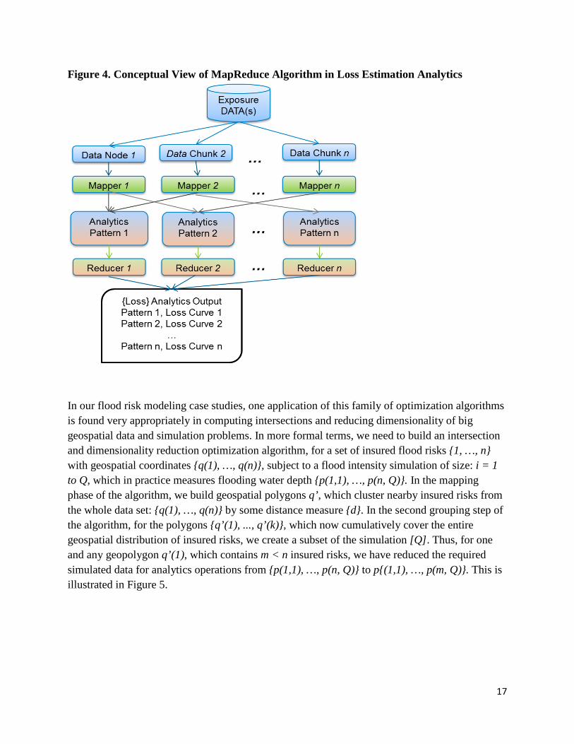
17

Figure 4. Conceptual View of MapReduce Algorithm in Loss Estimation Analytics

In our flood risk modeling case studies, one application of this family of optimization algorithms is found very appropriately in computing intersections and reducing dimensionality of big geospatial data and simulation problems. In more formal terms, we need to build an intersection and dimensionality reduction optimization algorithm, for a set of insured flood risks {1, …, n} with geospatial coordinates {q(1), …, q(n)}, subject to a flood intensity simulation of size: i = 1 to Q, which in practice measures flooding water depth {p(1,1), …, p(n, Q)}. In the mapping phase of the algorithm, we build geospatial polygons q’, which cluster nearby insured risks from the whole data set: {q(1), …, q(n)} by some distance measure {d}. In the second grouping step of the algorithm, for the polygons {q’(1), ..., q’(k)}, which now cumulatively cover the entire geospatial distribution of insured risks, we create a subset of the simulation [Q]. Thus, for one and any geopolygon q’(1), which contains m < n insured risks, we have reduced the required simulated data for analytics operations from {p(1,1), …, p(n, Q)} to p{(1,1), …, p(m, Q)}. This is illustrated in Figure 5.

18

Figure 5. Mathematics Workflow in Mapping and Reduction Algorithms

With this optimization approach, computing insured losses and correlation matrices within each polygon and subsequently for the entire geospatial distribution of risks becomes a much more manageable and sustainable proposition. Individual distributed computational resources are assigned to computing statistical, loss and risk metrics for each polygon, which is more effective and more economical than running the full simulation on a nonpartitioned and nondistributed compute resource.

5.4 Scheduling and Synchronization by Service Chaining

Distributed and service chaining algorithms process geospatial analysis tasks on data components simultaneously and automatically. For logically independent processes, such as computing intensities or losses on uncorrelated scenarios of a simulation, service chaining algorithms will divide and manage the tasks among separate computing resources. Dependencies and correlations among such data chunks may not exist because of large geospatial distances, as we saw in some of the modeling and pricing scenarios in our cases studies. Hence, they do not have to be modeled explicitly and performance improvements are gained immediately. For such scenarios, both input data and computational tasks can be broken down into pieces and subtasks respectively. For logically interdependent tasks, such as accumulations of interdependent quantities like losses in geographic proximity, chaining algorithms automatically order the commencement and completion of dependent subtasks.

In our modeled scenarios, the simulated loss distributions of risks in immediate proximity are accumulated first, where dependencies are expected to be the strongest. A second tier of accumulations for risks with partial dependence due to longer distances and full independence

19

measures is scheduled for once the first tier of accumulations of highly dependent risks is complete. Service chaining methodologies work in collaboration with autoscaling memory algorithms, which provide or remove computational memory resources, depending on the intensity of modeling and statistical tasks. Challenges still are significant in processing shared data structures. An insurance risk management example, which we are currently developing for our next working paper, would be pricing a complex multitiered product, comprised of many geospatially dependent risks, and then back-allocating a risk metric, such as TVaR, down to single risk granularity. On the statistical level, this back-allocation and risk management task involves a process called de-convolution or component convolution. A computational and optimization challenge is present when highly dependent and logically connected statistical operations are performed with chunks of data distributed across different hard data storage resources. Solutions are being developed for multithreaded implementations of MapReduce algorithms, which address such computationally intensive tasks. In such procedures, the mapping is done by task definition and not directly onto the raw and static data.

Some Conclusions and Further Work

With advances in computational methodologies for natural catastrophe and insurance portfolio modeling, practitioners are producing increasingly larger data sets of modeled physical, loss and risk metrics. Simultaneously, single product and portfolio optimization techniques are used in insurance premium underwriting, which take advantage of metrics in diversification and interrisk dependencies. Such optimization techniques significantly increase the frequency of production of insurance underwriting data, and require new types of algorithms, which can process multiple large, distributed and frequently updated sets. Such algorithms have been developed theoretically and now they are entering from a proof-of-concept phase in the academic environments to implementations in production in the modeling and computational systems of insurance firms.

Both traditional statistical modeling methodologies, such as premium pricing, and new advances in the definition of interrisk variance-covariance and correlation matrices and policy and portfolio accumulation principles require significant data management and computational resources to account for the effects of dependencies and diversification. Accounting for these effects allows the insurance firm to support cost savings in premium value for policyholders.

With many of the reviewed advances at present, there are still open areas for research in statistical modeling, single product pricing and portfolio accumulation, and their supporting optimal big insurance data structures and algorithms. Algorithmic communication and synchronization cost between global but distributed structured and dependent data is expensive. Optimizing and reducing computational processing cost for data analytics is a top priority for both scientists and practitioners. Optimal partitioning and clustering of data, and particularly so of geospatial images, is one other active area of research.

20

References

Ayma, V.A., R.S. Ferreira, P. Happ, D. Oliveira, R. Feitosa, G. Costa, A. Plaza, and P. Gamba. 2015. “Classification of Algorithms for Big Data Analysis, A Map Reduce Approach.” Remote Sensing and Spatial Information Sciences Conference paper.

Fedak, Gilles. 2013. “MapReduce Runtime Environments: Design, Performance, Optimizations.” INRIA/University of Lyon, France, presentation.

Goovaerts, Mark, and Roger Laeven. 2011. “Premium Calculation and Insurance Pricing.” Working paper, 3rd ed. https://feb.kuleuven.be/drc/AFI/research/AFIInsuranceFolder/InsurancePapers/2008-laeven-goovaerts.pdf.

Hurlimann, Werner. 2006. “On a Robust Parameter Free Pricing Principle: Fair Value and Risk Adjusted Principle.” White paper.

Song, W. W., B. X. Jin, S. H. Li, X. Y. Lei, D. Li, and F. Hu. 2015. “Building Spatiotemporal Cloud Platform for Supporting GIS Application,” ISPRS Annals of the Photogrammetry, Remote Sensing and Spatial Information Sciences (2015 International Workshop on Spatiotemporal Computing, July13–15, Fairfax, Va.) II-4/W2. https://www.isprs-ann-photogramm-remote-sens-spatial-inf-sci.net/II-4-W2/55/2015/isprsannals-II-4-W2-55-2015.pdf.

Isaac, Luke P. 2014. “Basics of Map Reduce Algorithm Explained with a Simple Example.” The Geek Stuff (blog). http://www.thegeekstuff.com/2014/05/map-reduce-algorithm/.

Nandakumar, A.N., and Nandita Yambem. 2014. “A Survey of Data Mining Algorithms on Apache Hadoop.” International Journal of Emerging Technology and Advanced Engineering 4, no. 1 (January). https://pdfs.semanticscholar.org/d4cb/64721dcbdcbcea40adbe6c29fa0c394c1b6d.pdf.

Nivranshu, Hans, Sana Mahajan, and S.N. Omkar. 2015. “Big Data Clustering Using Genetic Algorithm on Hadoop Mapreduce.” International Journal of Emerging Technology and Advanced Engineering 4, no. 04 (April). http://www.ijstr.org/final-print/apr2015/Big-Data-Clustering-Using-Genetic-Algorithm-On-Hadoop-Mapreduce.pdf.

Rau Chaplin, Andrew. 2015. “Scaling Up to Big Data: Algorithmic Engineering + HPC.” Statistical and Computational Analytics for Big Data Conference presentation. http://www.canssi.ca/wp-content/uploads/2015/07/Rau-ChaplinA.pdf.