compilation of measurement data - itu...compilation of measurement data relating to building entry...
TRANSCRIPT

Report ITU-R P.2346-1 (06/2016)
Compilation of measurement data relating to building entry loss
P Series
Radiowave propagation

ii Rep. ITU-R P.2346-1
Foreword
The role of the Radiocommunication Sector is to ensure the rational, equitable, efficient and economical use of the
radio-frequency spectrum by all radiocommunication services, including satellite services, and carry out studies without
limit of frequency range on the basis of which Recommendations are adopted.
The regulatory and policy functions of the Radiocommunication Sector are performed by World and Regional
Radiocommunication Conferences and Radiocommunication Assemblies supported by Study Groups.
Policy on Intellectual Property Right (IPR)
ITU-R policy on IPR is described in the Common Patent Policy for ITU-T/ITU-R/ISO/IEC referenced in Annex 1 of
Resolution ITU-R 1. Forms to be used for the submission of patent statements and licensing declarations by patent
holders are available from http://www.itu.int/ITU-R/go/patents/en where the Guidelines for Implementation of the
Common Patent Policy for ITU-T/ITU-R/ISO/IEC and the ITU-R patent information database can also be found.
Series of ITU-R Reports
(Also available online at http://www.itu.int/publ/R-REP/en)
Series Title
BO Satellite delivery
BR Recording for production, archival and play-out; film for television
BS Broadcasting service (sound)
BT Broadcasting service (television)
F Fixed service
M Mobile, radiodetermination, amateur and related satellite services
P Radiowave propagation
RA Radio astronomy
RS Remote sensing systems
S Fixed-satellite service
SA Space applications and meteorology
SF Frequency sharing and coordination between fixed-satellite and fixed service systems
SM Spectrum management
Note: This ITU-R Report was approved in English by the Study Group under the procedure detailed in
Resolution ITU-R 1.
Electronic Publication
Geneva, 2016
ITU 2016
All rights reserved. No part of this publication may be reproduced, by any means whatsoever, without written permission of ITU.

Rep. ITU-R P.2346-1 1
REPORT ITU-R P.2346-1
Compilation of measurement data relating to building entry loss
(2015-2016)
Scope
This Report provides a compilation of data on building entry loss, and is intended to supplement the material
in Recommendation ITU-R P.2040.
TABLE OF CONTENTS
Page
1 Introduction .................................................................................................................... 5
2 Building entry loss measurements (VHF & UHF, Europe)............................................ 5
3 Building entry loss measurements (5.2 GHz, Japan) ...................................................... 6
4 Exit loss measurements .................................................................................................. 6
4.1 Measured result ................................................................................................... 7
5 Slant path measurements (500 MHz - 6 GHz) ............................................................... 9
5.1 UHF satellite signal measurements (860 MHz – 2.6 GHz) ................................ 9
5.2 Slant-path measurements from towers or high rise buildings ............................ 10
5.3 Helicopter measurements to office building ....................................................... 14
5.4 Balloon measurements to domestic buildings (1-6 GHz) ................................... 19
6 Impact of thermally-insulating materials (88 MHz – 5.8 GHz) ..................................... 22
6.1 Introduction ......................................................................................................... 22
6.2 Median building entry loss ................................................................................. 22
6.3 Variability of loss within a room ........................................................................ 23
6.4 Variability of loss from room-to-room ............................................................... 24
6.5 Impact of insulating materials on loss ................................................................ 24
7 Measurements at 3.5 GHz .............................................................................................. 25
7.1 Environment ....................................................................................................... 25
7.2 Measurement configuration ................................................................................ 26
7.3 Measurement results at 3.5 GHz ......................................................................... 27
8 Measurements in Stockholm at 0.5 to 5 GHz ................................................................. 27
8.1 Configuration of the set-up ................................................................................. 27

2 Rep. ITU-R P.2346-1
8.2 General results .................................................................................................... 28
8.3 Average excess loss results ................................................................................. 29
8.4 Method 1 versus Method 2 results ...................................................................... 30
9 Building entry loss measurement at 3.5 GHz in Beijing ................................................ 31
9.1 Measurement scenarios ....................................................................................... 31
9.1.1 Building A ............................................................................................ 31
9.1.2 Building B ............................................................................................ 36
9.1.3 Building C ............................................................................................ 42
9.2 Test methodology ............................................................................................... 42
9.2.1 Measuring system and instrument ........................................................ 42
9.2.2 Calculation method of building entry loss ........................................... 42
9.3 Measurement results ........................................................................................... 43
9.3.1 Measurement results and analysis of building A scenario ................... 43
9.3.2 Measurement results and analysis of building B scenario ................... 46
9.3.3 Measurement results and analysis of building C scenario ................... 48
10 Building entry loss measurement at 3.5 GHz in UK ...................................................... 49
10.1 UK measurements ............................................................................................... 49
10.2 Methodology ....................................................................................................... 49
10.2.1 Hardware .................................................................................................. 50
10.2.2 Software ................................................................................................... 50
10.3 Test locations ...................................................................................................... 50
10.3.1 Terraced house ......................................................................................... 50
10.3.2 Small office .............................................................................................. 51
10.3.3 Retail buildings ........................................................................................ 52
10.4 Results ................................................................................................................. 53
10.4.1 Building entry loss ................................................................................... 53
10.4.2 BEL Variability ........................................................................................ 55
11 Building entry loss measurements at 28 GHz ................................................................ 56
11.1 Scenario .............................................................................................................. 56
11.2 Experimental Set-up ........................................................................................... 57
11.3 Data collection/analysis ...................................................................................... 58
11.4 Results ................................................................................................................. 58

Rep. ITU-R P.2346-1 3
11.5 Conclusion .......................................................................................................... 60
12 Measurements at 5.2 GHz .............................................................................................. 60
13 Building Entry Loss from 5-32 GHz .............................................................................. 61
13.1 Introduction ......................................................................................................... 61
13.2 Experimental Setup ............................................................................................. 61
13.2.1 Building descriptions ............................................................................... 63
13.2.2 Testing Locations ..................................................................................... 63
13.2.3 Data post processing ............................................................................... 67
13.3 Results ................................................................................................................. 67
13.3.1 Tabulated Results ..................................................................................... 67
13.3.2 Coverage maps ......................................................................................... 69
13.3.3 Distance dependency ............................................................................... 71
13.3.4 PDF Distributions .................................................................................... 73
13.3.5 CDF Distributions .................................................................................... 75
13.4 Tables of Building Parameters ............................................................................ 77
13.5 Conclusion .......................................................................................................... 79
14 Measurements at 3, 10 and 17 GHz ................................................................................ 80
14.1 Measurement Campaign ..................................................................................... 80
14.1.1 Scenario Description ................................................................................ 80
14.1.2 Setup and Procedure ................................................................................ 81
14.2 Data Processing .................................................................................................. 82
14.3 Measurement results and analysis ...................................................................... 85
14.3.1 Measurement validation (LoS cases) ....................................................... 85
14.3.2 Penetration Losses and Delay Spread ...................................................... 86
14.4 Conclusion .......................................................................................................... 91
15 Measurements in Stockholm in the 2-60 GHz frequency range ..................................... 92
15.1 Introduction ......................................................................................................... 92
15.2 Measurement campaign ...................................................................................... 92
15.3 Monte Carlo simulation of multi-pane glass window transmission loss ............ 95
16 Measurements at 5-31 GHz in China ............................................................................. 96
16.1 Measurement scenarios ....................................................................................... 96
16.1.1 Building A ................................................................................................ 96

4 Rep. ITU-R P.2346-1
16.1.2 Building B ................................................................................................ 102
16.2 Test methodology ............................................................................................... 109
16.2.1 Measuring system and instrument ........................................................... 109
16.3 Calculation method of building entry loss .......................................................... 110
16.4 Measurement results ........................................................................................... 111
16.4.1 Measurement results and analysis of Building B scenario ..................... 112
17 Measurements below 6 GHz in a modern office building .............................................. 113
17.1 Method ................................................................................................................ 113
17.2 Locations ............................................................................................................. 113
17.3 Measurement procedure ...................................................................................... 116
17.4 Reference measurements .................................................................................... 117
17.5 Results ................................................................................................................. 120
17.5.1 Building entry loss (median loss) ........................................................................ 120
17.5.2 Building entry loss statistics ................................................................................ 122
17.6 Conclusions ......................................................................................................... 123
17.7 Annex – link budgets .......................................................................................... 123
17.8 Annex – measurement zones at Riverside House ............................................... 124
18 Building loss in an urban environment (Japan, 0.8-37 GHz) ......................................... 126
18.1 Measurement methods and parameters ............................................................... 126
18.2 Measurement results from 0.8 to 37.1 GHz band ............................................... 128
Annex 1 – Building entry loss in point-to-area applications below 3 GHz ............................. 131

Rep. ITU-R P.2346-1 5
1 Introduction
This Report provides a compilation of empirical data on building entry loss (BEL), and is intended
to support the material in Recommendation ITU-R P.2040.
It is also expected that the material in this Report will be of value in the development of new
propagation models.
Annex 1 provides information that has been found helpful in planning broadcast and other point-to-
area radio services at frequencies below 3 GHz. The contents of this Annex encapsulate
measurement data but do not report on a specific measurement campaign.
It should be noted that the measurements recorded in this report have been made using a wide
variety of methods. In particular, the definition of BEL may differ from that given in
Recommendation ITU-R P.2040. Readers are advised to evaluate the material carefully to ensure
that it is appropriate for the purpose intended.
2 Building entry loss measurements (VHF & UHF, Europe)
Measurements have been carried out in Germany and the United Kingdom to determine values of
BEL and other parameters to be used in planning indoor reception of broadcasting services.
The German measurements were made at two frequencies in the VHF band used for digital audio
broadcasting and two frequencies in the UHF band. The median values of the BEL over all
measurements made in buildings typical for Germany were 9.1 dB at 220 MHz, 8.5 dB at 223 MHz,
7.0 dB at 588 MHz and 8.5 dB at 756 MHz.
The penetration loss from the front of the building (the side with higher signal level) into a room
on the opposite side has median values of 14.8 dB at 220 MHz, 13.3 dB at 223 MHz, 17.8 dB at
588 MHz and 16 dB at 756 MHz.
Over all measurements, the median values of the location variation standard deviations are 3.5 dB
for the 220 and 223 MHz signals with 1.5 MHz bandwidth and 5.5 dB for the 588 and 756 MHz
signals with 120 kHz bandwidth.
The United Kingdom measurements were made at a number of frequencies in the UHF band.
The median BEL at UHF was found to be 8.1 dB with a standard deviation of 4.7 dB. However, the
value for rooms on the side of the building furthest from the transmitter was 10.3 dB, whereas the
corresponding value for rooms on the side of the building nearest to the transmitter was 5.4 dB; a
difference of about 5 dB.
A median value of 13.5 dB was measured for the outdoors height gain between 1.5 and 10 m.
The locations of the measurements were suburban.
The median value of the difference in field strength between ground floor and first floor rooms was
found to be 5.4 dB.
The standard deviation of the variation of field strength within rooms was about 3 dB.
The standard deviation of the variation of field strength measured for a floor of a house was about
4 dB.
Despite differences in the frequencies and bandwidths of the measurements, there is very good
agreement between the German and United Kingdom measurements.

6 Rep. ITU-R P.2346-1
3 Building entry loss measurements (5.2 GHz, Japan)
Entry loss measurements were made in Japan on 12 office buildings at distances from the
transmitter of up to 1 km.
The additional path loss to points within a building was measured relative to the outdoor field
averaged along a path around the building at 1.5 m height. Note that the use of the fixed height
reference differs from the definition of building entry loss given in Recommendation ITU-R
P.2040, and will lead to negative values of entry loss for higher floors of the building.
The data from these measurements has been fitted by the following expression for excess path loss
with respect to the averaged 1.5 m value:
5.118.0log1.25.041.0)dB( LoSfhdLoss (1)
where:
d : 0 to 20 m; the distance from the window (m);
h : 1.5 to 30 m; the height from the ground (m);
f : 0.8 to 8 GHz; the frequency (GHz);
LoS : 1 for line-of-sight, LoS = 0 for non-line-of-sight.
4 Exit loss measurements
Figure 1 shows a picture of the house used in the measurement. It is a typical bi-level frame house
in Japan. The site is approximately 11 m × 12 m. The outer walls have two or three windows on
each side. The outside of the exterior walls is covered by painted wooden boards and the inside of
the walls are covered with plasterboard. Glass fibre insulation fills the space between inside the
walls. A transmitting antenna is set near the centre of the lower floor. The antenna height above the
floor level is 1.5 m. A 5.2-GHz continuous wave is transmitted from a vertically polarized dipole
antenna. A receiver connected to a dipole antenna is set on a pushcart and moved around the house.
The receiving antenna height is set at 2.2 m from the ground level to make it equal in height to the
transmitting antenna. Before conducting outside measurements, the received level is measured at
several points inside the house.
FIGURE 1
Photo of house
P.2040-29

Rep. ITU-R P.2346-1 7
4.1 Measured result
Figure 2 is a contour map of the received level. High levels are expressed as dark colour and low
levels are expressed as light colours. The map shows that intense radiowaves spread out through the
windows and propagate to relatively far distances. In this figure, the white part in the upper right
corner indicates the location where we could not take measurements due to a barn. The other white
part in the upper left side is due to a hedgerow.
FIGURE 2
Contour map of the received level
P.2040-30
0 2 4 68 10 12 14 16 18 (m)
Entrance
01
3
5
7
9
11
13
15
17
19
21
23
25
27
29
31
33
35
37
39
0 2 4 6 8 10 12 14 16 18
(m)
(m)
41
11
13
15
17
19
21
23
25
27
29
31
33
35
37
39
41
(m)
Photo
Window
–100 – –97 –97 – –94 –94 – –91 –91 – –88 –88 – –85 –85 – –82 –82 – –79 –79 – –76 –76 – –73(dBm)
Tx
Figure 3 shows the distance dependency of the path loss. The abscissa is a linear scale. The blue
circles represent outdoor data and the red triangles represent indoor data. The path loss is
approximated by the following equation.
L(dB) = 20log (f (MHz)) + N log(d(m)) – 27.55 + Lf (dB) (2)
where N is the attenuation coefficient for distance and Lf is the additional attenuation caused by wall
penetration for example. When N and Lf equal 20 and 0, respectively, this equation expresses the
free-space path loss.

8 Rep. ITU-R P.2346-1
Three calculated lines are shown in Fig. 3. The black dashed line is the free-space path loss at
5.2 GHz. The red solid line approximates the indoor data set. Its Lf equals zero but N equals 30 for a
large decline compared to that for free space. The blue solid line has N = 20 and Lf = 15. The curve
parallels that for free-space curve but with a drop of 15 dB. This result indicates that the path loss
increases with a large N within the house and the increase becomes gradual after it exits the house.
This feature is clearly observed in Fig. 3.
FIGURE 3
Distance dependencies of the path loss (linear scale)
P.2040-31
Distance from (m)Tx
0 5 10 15 20 25 30 35 40100
90
80
70
60
50
Path
loss
(dB
)
N L
N L
= 20, = 0
= 20, = 15
f
f
N L = 30, = 0f
Indoor
Outdoor
Based on these data, cumulative probabilities of the path loss are derived in Fig. 4. The difference
between these two probabilities is approximately 18 dB. This indicates that the radiowave exits
from the house with an attenuation of approximately 18 dB and propagates with the same
attenuation coefficient in distance as that for free space.

Rep. ITU-R P.2346-1 9
FIGURE 4
Cumulative probabilities of measured path loss data
P.2040-32
L (dB)
55
Cu
mu
lati
ve p
robab
ilit
y (
%)
60 65 70 75 80 85 90 95.01
.1
1
5102030
50
70809095
99
99.9
99.99
IndoorOutdoor( < 10 m)d
18 dB
5 Slant path measurements (500 MHz - 6 GHz)
5.1 UHF satellite signal measurements (860 MHz – 2.6 GHz)
Representative UHF satellite signal attenuation observed within rooms located near an exterior wall
in timber-framed private homes is summarized in Table 1. For interior rooms, 0.6 dB must be added
to the tabulated values. For timber-framed buildings the attenuation shows little variation with
weather or path elevation angle but, as the Table illustrates, there is a systematic variation with
frequency, polarization, construction materials, insulation and position within the structure. Some
aluminium-backed insulating and construction materials contribute up to 20 dB of loss.
TABLE 1
UHF signal attenuation (dB) through timber-framed buildings*
Building condition Frequency (MHz) and polarization
(Horizontal: H, Vertical: V)
Exterior Insulation
(non-metallic
type)
860 H 860 V 1 550 V 2 569 V
Wood siding Ceiling only 4.7 2.9 5.0 5.8
Ceiling and wall 6.3 4.5 6.6 7.4
Brick veneer Ceiling only 5.9 4.1 6.2 7.0
Bricks Ceiling and wall 7.5 5.7 7.8 8.6
* The Table is for rooms located near to the exterior wall; for interior rooms, 0.6 dB should be added.

10 Rep. ITU-R P.2346-1
5.2 Slant-path measurements from towers or high rise buildings
Measurements of building entry loss using 18 to 20 m towers to simulate a satellite transmitter were
performed in the bands 700 MHz to 1.8 GHz and 500 MHz to 3 GHz to determine the mean loss
and spatial variability in a variety of buildings. There are insufficient data to give precise prediction
methods, but the data in Tables 2 to 3 are indicative.
TABLE 2
Signal distributions at the average position and best position within buildings
(over the frequency range 700 to 1 800 MHz)
Building
number Construction Elevation angle
Average position Best position
Mean
loss
(dB)
Standard
deviation
(dB)
Mea
n
loss
(dB)
Standard
deviation
(dB)
1 Corner office, large
windows, single-story
building. Concrete block,
plasterboard, double-glazing.
Concrete roof on steel beams
27.5 (LoS
through window,
azimuth angle
between wall and
LoS is 50)
7.9 5.5 4.2 4.2
2 Small room with windows
being 5/8 of exterior wall 18 (LoS through
window, azimuth
angle between
wall and LoS is
50)
9.1 4.4 5.4 3.7
3 Corner foyer, large reflective
glass door in half of one
exterior wall. External walls
concrete, internal walls
plasterboard on metal frame
16 (LoS through
window, 45
azimuth angle
between one wall
and LoS, both
exterior walls
illuminated by
transmitter)
15.4 8.4 9.7 6.7
4 Sheet metal shack with
plywood interior. One small
unscreened window on each
of two sides, metal-covered
door
25 (azimuth
angle between
wall and LoS is
60)
9.7 6.3 5.2 4.9
5 Two-story wood-side house,
rockwool insulation (walls
and attic); gypsum board, no
metallic heat-shield. No
metallic screens on windows.
Wood-shingled roof
25 (azimuth
angle between
wall and LoS is
45)
9.0 4.5 5.4 3.7
6 Empty sheet-metal mobile
trailer home, metal frame
windows with metal screens
25 (azimuth
angle between
wall and LoS is
45)
24.9 3.8 19.8 3.4

Rep. ITU-R P.2346-1 11
TABLE 3
Median loss at the average position and best position within buildings
as a function of frequency
(Construction details and elevation angle as in Table 2)
Building number Average position Best position
(As in Table 2) 750-1 750 MHz 750-1 750 MHz
1 5-11 dB 2-6 dB
2 5-14 dB 2-5 dB
3 17-18 dB 12-13 dB
4 9-11 dB 5-6 dB
5 5-11 dB 3-5 dB
6 20 to > 24 dB 16-22 dB
TABLE 4
Signal distributions at the average position within buildings
(estimated over the frequency range 500-3 000 MHz)
Building
number Construction
Elevation angle
(degrees)
Average position
Mean loss
(dB)
Standard
deviation
(dB)
1 Entry lobby in single storey building –
concrete tilt wall, tar roof
18 13 10
2 Office in single storey building –
block brick, tar roof
38 9 7
3 Two-storey wood frame farmhouse,
metal roof, no aluminium heat-shield
33 5 4
4 Hallway and living room of two-storey
woodframe house, metal roof,
aluminium heat-shield
41 19.5 12
5 Motel room in two-storey building,
brick with composite roof
37 13 6
6 Lobby of two-storey building, glass
and concrete, tar roof
26 12 5
In the first set of measurements (Tables 2 and 3), the first three buildings had elevation angles such
that the room was illuminated through a window with a direct LoS from the transmitter. The
elevation angles were below 30° to allow side illumination of the buildings.
In the case of building number 3 in these tables, losses through the reflective glass door were about
15 dB greater than when the door was open.
The results of another study are similar, with mean attenuation levels (in the frequency range
500 to 3 000 MHz) varying between 5 dB for a woodframe house with metal roof and no aluminium
heat-shield, to 20 dB for a similar house with an aluminium heat-shield. Table 4 shows a summary
of the measured mean attenuation values.

12 Rep. ITU-R P.2346-1
Note that for some of the measurements, values obtained near a window or an open door, are
included in the averaging. In the motel (building 6), attenuation when the direct path penetrated a
brick wall was 15 to 30 dB below the LoS value. Levels inside building 4 varied from 25 to 45 dB
below the LoS value, due to the metal roof and aluminium heat-shield.
Note also that the measurements were on stationary paths. There is evidence that close-in multipath
effects will give rise to fluctuations in received signal level should the transmitter or receiver move.
This has implications particularly for low-Earth orbit (LEO) systems where the transmitter is
moving rapidly with respect to the receiver.
The measurements indicate that attenuation increases with frequency by about 1 to 3 dB/GHz in
buildings 1, 2, 4, and 6, by 6 dB/GHz in the least attenuating building (building 3), and shows
almost no change with frequency in the glass-walled building 5. Since the values given above are
averaged over the frequency range 500 MHz to 3 GHz, they are expected to be slightly optimistic
for the 1 to 3 GHz range.
For the six buildings identified in Table 2, 1.6 GHz and 2.5 GHz measurements were performed and
analysed to determine the median, 5% and 95% levels of relative signal loss when the antennas
were moved horizontally over multiple 80 cm intervals. The buildings were illuminated from the
side, and the signals received inside the outside wall (one-wall entry). Azimuthally omnidirectional
antennas were used to receive the transmitted signals. Statistics derived from these measurements
are summarized in Fig. 5. These data indicate the magnitude and variations of fading that are
possible for signal transmission through building walls. Note that on occasions, multipath
conditions yield relative signal levels in excess of 0 dB.

Rep. ITU-R P.2346-1 13
FIGURE 5
Median, 5% and 95% levels of building entry power loss relative to unobstructed LoS at 1.6 GHz and 2.5 GHz for the six
buildings identified in Table 2 (designated by 1 to 6 in the Figure).
For each building, the 1.6 GHz (L) and 2.5 GHz (S) statistics are shown separately
None of the available measurements at frequency bands below 3 GHz provides information for
elevation angles above 41°. However, the large losses through metal structures (building 6 in
Tables 2 and 3; building 4 in Table 3) suggest that attenuation for a direct path through a metal roof
will be of the order of 20 dB. The losses of 15 to 30 dB for a brick wall in building 4 of Table 3 are
relevant for higher elevation angles as well.
The elevation angle dependence of building entry loss was measured in the 5 GHz band at two
different elevation angles by using high-rise buildings to simulate the reception of satellite signals.
In an office-type room, the measured medians of the excess building entry loss were 20 dB and
35 dB for elevation angles of 15° and 55°, respectively.
P2040-24
1 2 3 4 5 6–60
–50
–40
–30
–20
–10
0
10
20
L
S
S
L
Frequency band and building number
Sig
nal
-lev
el r
elat
ive
to c
o-p
ola
rize
d c
lear
pat
h (
dB
)
Nominal range of measured values 95% - 5% Median
L
S
L S
LS L
S

14 Rep. ITU-R P.2346-1
5.3 Helicopter measurements to office building
The elevation and azimuth angle dependencies of building entry loss around 5 GHz were measured
at different positions within an eight-storey building on three different floors. A helicopter was used
to simulate a satellite transmitter. The received signal was continuously recorded, as well as the
position of the helicopter by means of a differential global positioning system (GPS) receiver. The
experimental conditions and averaged measurement results are summarized in Table 5. The
behaviour of the building entry loss with respect to path elevation angle is shown in Fig. 6, and the
behaviour with respect to azimuth in Fig. 7 for elevation angles of 15° and 30°.

Rep. ITU-R P.2346-1 15
FIGURE 6
Building entry loss at 5.1 GHz at sections 1, 2 and 3 for floors 2, 5 and 6. The angle E is
positive-defined when looking to the north and negative-defined to the south
90E where ε is the elevation angle
P.2040-25
Building section 1
–90 –70 –50 –30 –10 10 30 50 70 900
5
10
15
20
25
30
35
40
45
Bu
ild
ing
entr
y lo
ss (
dB
)
Elevation angle (degrees)E
Building section 2
–90 –70 –50 –30 –10 10 30 50 70 900
5
10
15
20
25
30
35
40
45
Bu
ild
ing
entr
y lo
ss (
dB
)
Elevation angle (degrees)E
Building section 3
–90 –70 –50 –30 –10 10 30 50 70 900
5
10
15
20
25
30
35
40
45
Bu
ild
ing
entr
y l
oss
(dB
)
Elevation angle (degrees)E
Floor 2
Floor 5
Floor 6
Building section 1: rooms with windows facing helicopter transmitter.
Building section 2: center of corridor.
Building section 3: rooms with windows not facing helicopter transmitter.

16 Rep. ITU-R P.2346-1
FIGURE 7
Building entry loss at 5.1 GHz for elevation 15° and 30° at the four different indoor antenna positions.
Numbers 1 and 2 are located close to an outer wall, whereas numbers 3 and 4 are located in the corridor
P.2040-26
0
Azimuth (degrees) 0 = East
Buil
din
g e
ntr
y l
oss
(d
B)
5
10
15
20
25
30
35
40
0 50 100 150 200 250 300 350
Position 1
0
Azimuth (degrees) 0 = East
Buil
din
g e
ntr
y l
oss
(d
B)
5
10
15
20
25
30
35
40
0 50 100 150 200 250 300 350
Position 2
0
Azimuth (degrees) 0 = East
Buil
din
g e
ntr
y lo
ss (
dB
)
5
10
15
20
25
30
35
40
0 50 100 150 200 250 300 350
Position 3
0
Azimuth (degrees) 0 = East
Buil
din
g e
ntr
y lo
ss (
dB
)
5
10
15
20
25
30
35
40
0 50 100 150 200 250 300 350
Position 4
4545
Elevation 15°
Elevation 30°

Rep. ITU-R P.2346-1 17
TABLE 5
Average median building entry loss and observed range of the median building entry
loss measured at 5.1 GHz for different positions in an office building
Type of
measurements
(helicopter
trajectory)
Average of the median
building entry loss for
different receiver
positions in the
building
(dB)
Observed range
of the median
building entry
loss
(dB)
Eight-storey building with seven
storeys above ground and one extra
storey placed on the former roof,
brick-walls and windows placed in
strips: behind the brick-wall there is a
10 cm thick concrete wall; windows
made of two layers of plain non-
thermal glass, storeys separated by
3.5 m with 2.5 m from floor to
ceiling, two layers of plaster with
wooden laths in between separate the
rooms; interior walls facing the
corridor are in most cases made of
glass, rooms commonly furnished
with desks and bookshelves; each
storey has three sections, a corridor
with office rooms at the sides
Elevation angle
measurements
(linear,
perpendicular to
the long side of
the building)
19.1 ~ 5-45
Azimuth angle
measurements
(circular at
elevation angles
of 15 and 30)
22.3 ~ 10-42
Measurements at 2.57 GHz and 5.2 GHz using an igloo shaped flight pattern were performed
inward to three different buildings, one of them in the Graz/Austria area, another two in the
Vienna/Austria area, covering various building types. The transmitter was carried by a helicopter,
on which a steerable helix antenna was mounted. The measurements were performed with a high
resolution, pseudo random sequence based channel sounder with a chipping rate of 100 Mcps and
200 MHz bandwidth. The transmit antenna was right-hand circularly polarized (RHCP) while the
receive antenna for the channel sounder case consisted of a set of patch antennas with two
orthogonal linear polarizations covering a surface that approximates a semi-sphere.
Table 6 gives an overview of the inward building locations.
TABLE 6
Overview on buildings measured
Building Location #RX
locations Façade/roof material
Millennium
Tower
skyscraper
22nd floor
44th floor
Vienna 2
2
Metal grid and glass panels,
coated glass with sun protective
layer/Reinforced concrete
Graz airport Gate Area
Conference room
Feldkirchen
near Graz
4
1
Steel, metal construction
elements, coated glass with sun
protective layer/Steel, metal
sheets, layer of gravel
Office
building FFG
Inner city office
building, highest floor
Vienna 2 Reinforced concrete/coated
windows

18 Rep. ITU-R P.2346-1
The building entry loss shown in Table 7 was calculated by subtracting the Average Power Delay
Profile from an outdoor reference measurement from the Average Power Delay Profile
measurement inside the buildings. The building entry loss for various distances to the window
directed to the transmitter at 5.2 GHz is presented in Table 8.
TABLE 7
Entry loss (dB) for different elevation and relative azimuth angles at 2.57 and 5.2 GHz
Building
Relative
azimuth to
facade
normal
2.57 GHz 5.2 GHz
Elevation Elevation
15 30 45 60 15 30 45 60
Millennium
Tower
44th floor
0 22.86 24.42 21.53 23.95 30.40 27.65 32.09 29.77
–30 22.13 22.17 25.21 24.59 28.34 30.42 32.43 33.31
–60 24.44 23.71 25.91 24.60 29.00 31.31 33.57 34.97
–90 25.40 29.24 27.21 26.77 32.65 34.23 37.24 38.21
Millennium
Tower
22nd floor
0 28.04 28.31 28.13 28.28 36.53 37.55 35.38 39.45
–30 28.70 29.60 29.60 27.59 31.84 36.57 37.51 35.34
–60 32.26 33.17 33.66 35.38 35.19 37.12 35.90 39.65
–90 35.30 42.22 37.80 – 43.20 43.80 47.02 46.52
Office
Building
0 21.69 29.23 26.18 31.40 26.52 31.13 34.13 35.28
30 26.49 34.90 31.10 33.00 33.12 33.49 36.51 34.08
60 27.43 – 35.90 36.13 34.29 34.16 36.30 35.73
90 – 38.09 – – – – – –
Airport –
Gate Area
0 18.18 – 23.68 23.00 28.36 35.76 – 37.97
–30 15.09 21.12 19.11 27.10 – – – 37.98
–60 18.25 26.13 21.96 25.42 27.67 37.76 – –
–90 – 27.71 23.69 24.61 34.31 – – –
Airport –
Conference
Room
0 11.81 12.62 – 10.84 15.19 19.68 19.37 19.09
–30 11.69 – 15.05 13.63 17.73 19.37 20.03 –
–60 16.65 17.87 17.66 16.35 22.79 – 24.70 22.38
–90 18.52 20.10 17.43 – 25.17 24.32 23.43 –

Rep. ITU-R P.2346-1 19
TABLE 8
Entry loss (dB) at 5.2 GHz for different elevation angles relative to the
distance to the window directed to the transmitter located
at 0 degrees relative azimuth angle to the façade normal
Building
Distance to
window
(m)
Elevation
15 30 45 60
Millenium Tower
44th floor
1.4 – 25.30 31.41 27.80
2.4 – 27.34 31.16 27.81
3.4 – 29.72 31.64 30.58
4.4 – 25.6 32.19 28.88
5.4 30.40 29.08 33.43 30.34
Airport – Gate Area 0.5 30.63 35.07 – 38.72
2.5 30.28 35.01 – 37.09
4.5 29.97 35.96 – 38.03
6.5 16.40 36.85 – –
5.4 Balloon measurements to domestic buildings (1-6 GHz)
Measurements have been made in the United Kingdom of building entry loss into a number of
domestic buildings of traditional construction. These measurements were made at 1.4 GHz,
2.4 GHz and 5.8 GHz, and used a tethered balloon to explore a range of elevation angles.
Details of measurement locations are given in Table 9.
TABLE 9
Building Date Measurement locations
Small offices/flats (3 floors) 1985 Measurements in two offices (1st floor)
Detached house (3 floors) 1905 Kitchen (ground) and bedroom (1st floor)
Terraced house (2 floors and
attic)
1880 Living room (ground), Bedroom (1st floor) and study
(2nd floor)
Terraced house (2 floors) 1965 Dining room & living room (ground), hallway (1st floor)
The measurements were made using CW transmitters suspended from a tethered helium balloon,
which allowed elevation angles up to around 70º to be explored. The receiver was switched between
an indoor measuring antenna and an external reference antenna. The measuring antenna was moved
along a 1 m track under computer control, to allow spatial averaging of measurements.
Omnidirectional antennas were used at both transmitter and receiver, and corrections were applied
for antenna vertical radiation patterns, and the difference in free-space loss between the reference
and measuring antennas.
Following the corrections described above, a data set giving the mean penetration loss for each test
location was obtained. The cumulative distribution function (CDF) of these results is shown in
Fig. 8, and represents the statistics of mean local loss with respect to all 11 receiver locations, at all
elevation angles. The receiver locations were randomly chosen and were almost entirely NLoS to
the balloon.

20 Rep. ITU-R P.2346-1
FIGURE 8
Overall statistics of building entry loss
P.2040-27
Building loss (dB)
–5 5 15 25 350.001
0.01
0.1
1
Pro
bab
ilit
y Overall
1.3 GHz
2.4 GHz
5.7 GHz
The mean value of building entry loss, at all frequencies, is 11.2 dB. The results shown in Fig. 7
show a slight frequency dependence in the results. Mean values of penetration loss are 9.2 dB at
1.3 GHz, 11.2 dB at 2.4 GHz and 12.7 dB at 5.7 GHz.
Figure 9 shows the elevation dependence of the measurements (polynomial curves fitted to
measurement points).
FIGURE 9
Mean values for each frequency compared
P.2040-28
0 10 20 30 40 50 60 70 80
Path elevation (degrees)
0
5
10
15
20
Bu
ildin
g l
oss
(d
B)
1.3 GH z
2.4 GH z
5.7 GH z
1.3 GH z subset
Dependence on path elevation
The results at 1.3 GHz show an anomalous increase in the penetration loss for higher elevation
angles. Examination of the measurement data shows that this effect is due to one set of
measurements and the effect of excluding this data is shown in the dotted curve.

Rep. ITU-R P.2346-1 21
It can be seen that, except at the lowest frequency, there is a slight decrease in penetration loss for
higher elevation angles. This decrease in building loss with elevation runs counter to the
assumptions made in some previous models. It may be that this behaviour is characteristic of
domestic buildings, where floors and ceilings are typically of light wooden construction.
Some dependence, of the averaged results, on the building floor is apparent, with the ground floor
and first floor results generally showing some 5-8 dB greater loss than those for the second floor. It
should be borne in mind, however, that only one set of measurements was made on a second floor,
and the location was a converted roof space, used as a home office.
Building shadowing loss measurements
Measurements have been carried out in Australia to determine values of building shadowing loss to
be used in planning frequency sharing between the fixed-satellite service and the fixed service.
The building shadowing loss is defined as transmission loss through a building.
The frequency is 11 GHz. Polarization is vertical and horizontal.
Table 10 shows the average results of measurements at 11 GHz through the different types of
buildings.
TABLE 10
Mean and standard deviation of loss by polarization and building type
Test site Avg. loss (V-Pol) Std. dev. Avg. loss (H-Pol) Std. dev.
1 Wooden building (lengthways) 26.4 dB 7.1 – –
1A Wooden building (widthways) 10.0 dB 7.0 8.3 dB 5.0
2 Concrete/brick building 30.1 dB 5.0 28.6 dB 5.5
3 Metal shed 36.4 dB 4.1 35.0 dB 3.2
The measurements show a high dependence on construction material in determining:
– the primary mode of propagation; and
– the amount of attenuation caused by the obstacle.
Wooden construction materials caused the lowest average attenuation of 10.0 to 25.0 dB, brick and
concrete between 25.0 and 35.0 dB and metal between 35.0 and 40.0 dB. The primary mode of
propagation for wooden and concrete structures was transmission, while the dominant mode of
propagation for metal structures was propagation by diffraction.
During propagation by diffraction, there was a high dependence on diffraction angle. As the
diffraction angle increased from the corners (i.e. towards the centre of the building shadow) the
amount of attenuation due to diffraction increased (on the order of 5.0 to 10.0 dB).
Although there was dependence on polarization at each measurement point, there was little to no
dependence on polarization or path length from the standpoint of averaged data. The average
attenuation variation between horizontal and vertical polarizations was less than 1.5 dB.
Wooden construction materials caused the lowest average attenuation of 10.0 to 25.0 dB, brick and
concrete between 25.0 and 35.0 dB and metal between 35.0 and 40.0 dB. The primary mode of
propagation for wooden and concrete structures was transmission, while the dominant mode of
propagation for metal structures was propagation by diffraction.
During propagation by diffraction, there was a high dependence on diffraction angle. As the
diffraction angle increased from the corners (i.e. towards the centre of the building shadow) the
amount of attenuation due to diffraction increased (on the order of 5.0 to 10.0 dB).

22 Rep. ITU-R P.2346-1
Although there was dependence on polarization at each measurement point, there was little to no
dependence on polarization or path length from the standpoint of averaged data. The average
attenuation variation between horizontal and vertical polarizations was less than 1.5 dB.
6 Impact of thermally-insulating materials (88 MHz – 5.8 GHz)
6.1 Introduction
A large body of measured data already exists and this study could add only a small amount to this.
The focus was therefore on a careful assessment of the impact of well-characterised changes to
building insulation.
A series of measurements have been undertaken on a small detached house; measurements of entry
loss were made to the un-modified structure, with metalised windows and when fitted with
foil-backed plasterboard. A further set of measurements was also made with window apertures
covered in foil, as a diagnostic experiment, and to test the sensitivity to different incidence angles.
Measurements were also made in a contrasting building – a much larger Victorian structure
(‘The Mansion’).
Measurements made at five frequencies: 88 MHz, 217 MHz, 698 MHz, 2 410 MHz and 5 760 MHz;
in the trials, a transmitter was carried so as to fully explore each room in a semi-random manner,
with received field strength being logged at an outdoor receiver positioned some 30-50 m from the
building. Each room in a building was characterised in terms of the median signal level, and this
was related to the field immediately outside the building at the same height to determine the
building entry loss.
6.2 Median building entry loss
Overall summary results are given in the figure below (in which ‘win1’ and ‘win2’ indicates
the fitment of different metalised windows and ‘FBP’ of foil-backed plasterboard). All curves relate
to measurements in the small, modern, house except for the single curve identified as ‘mansion’.
FIGURE 10
Overall summary building entry loss results

Rep. ITU-R P.2346-1 23
The relatively high losses seen at 88 MHz appear to be an anomalous feature of the small house;
the effect was not seen when a path between terminals was more oblique with respect to the front
wall of the house (although the results for 698 MHz now seem anomalous, illustrating the
complexity of the mechanisms involved).
6.3 Variability of loss within a room
Data has also been gathered on signal variability, which is significantly higher inside buildings due
almost entirely to multipath effects. Figure 10 shows time-series1 of measurements at 88 MHz and
5.7 GHz (bottom), illustrating the variability of signals within one room of the house, compared
with the variability measured over an equivalent outdoor area.
FIGURE 11
Measurements made indoors (blue) and outdoors (red) – see text
The results at both frequencies show similar trends. The inside signals are weaker on average due
to the attenuation of the building. It is also clear that there is more variability on the measurements
from inside the building. This is as expected because the inside environment is more rich in
multipath than the outside environment. The standard deviations at 88 MHz are 5.5 dB (inside)
and 1.8 dB (outside) and at 5.7 GHz are 6.8 dB (inside) and 3.8 dB (outside).
1 Sampled at equal time-intervals; the faster pace of measurement outdoors resulted in fewer samples being
collected.

24 Rep. ITU-R P.2346-1
These standard deviations relate mainly to signal variability due to multipath and a small
contribution (less than a decibel) due to the path length variation over the measurement area.
6.4 Variability of loss from room-to-room
The standard deviation of the room median building entry loss values are shown in Fig. 12 for the
different building configurations. There is no very useful frequency trend. The results for the small
house configurations are reasonably consistent for type 1 glass, with type 2 glass and the artificial
foil-over-windows cases showing some differences. The standard deviation is generally higher in
the mansion.
FIGURE 12
Room to room standard deviation of building entry loss
The room-to-room standard deviations are about half the values obtained for the signal variability
within the living room alone. This is as expected because multipath has been removed in
the room-to-room calculation. However the significant difference between the two buildings
suggests that a good measure of ‘variability’ really needs to take account of a larger population
of building types.
It is not clear that any adequate model yet exists to characterise this variability.
6.5 Impact of insulating materials on loss
The measurements show increasing levels of building entry loss as modern insulating materials
are added to an uninsulated house (see Fig. 13).

Rep. ITU-R P.2346-1 25
FIGURE 13
Increase in BEL compared to baseline configuration
For a small house, a combination of foil-backed insulation and metalised double glazed windows
(representative of a well-insulated property), added 5-10 dB to the building entry loss. The losses
increase with frequency, but most of the increase is accounted for in the uninsulated configuration
and the additional loss due to the insulating materials shows relatively weak frequency dependence.
An additional 5 dB of screening was obtained when, in addition, all windows and door apertures
were covered by foil; this might approximate to a ‘worst case’ whole building figure for building
entry loss.
7 Measurements at 3.5 GHz
7.1 Environment
Concrete and glass are two typical materials for the building.
In this paper, these two materials are measured.
For the concrete material, 50 cm width * 100 cm length * 10 cm thickness concrete slab is tested.
The test environment is an anechoic chamber in Tsinghua University, Beijing, China.
For the class material, the measurement field was located at the FIT building, Tsinghua University
in Beijing, China. The FIT building is a typical office building full of coated glass, the overall
window to wall ratio is more than 2:1. The building height is about 20 m. Coated glass offers
enhanced benefits to buildings, partitions, skylights, curtain walls, and other applications. Annex 2
also provides similar material’s building entry loss results.
The characteristics of the environment scenario are shown in Tables 11 and 12.
TABLE 11
Environment characteristics for the concrete scenario
Characteristics
Location Anechoic chamber in Tsinghua University
Building type Basement room
Object of the measurement Normal concrete slab
Thickness of the concrete slab 10 cm and 20 cm

26 Rep. ITU-R P.2346-1
The measurement object is the concrete slab in the middle of the transmitter and receiver antenna.
The thickness is about 10 cm.
TABLE 12
Environment characteristics for the glass scenario
Characteristics
Location FIT building East hall, Tsinghua University, Beijing, China
Building type Office
Object of the measurement The coated glass between the FIT building hall and the centre garden
Thickness of the glass Total 10 mm (two 2 mm glass plus 6 mm inner gap)
Height of buildings About 20 m
Surrounding Typical office building which full of glass, window-to-wall ratio is more
than 2:1.
The measurement object is the glass between the FIT building hall and the centre garden. The glass
is typical large two layer class in which the total thickness is about 10 mm including the inner gap.
Note that 7 cm width metal pillars connect adjacent glass panels.
7.2 Measurement configuration
The measurement configuration parameters are shown in Table 13.
TABLE 13
Measurement configurations
Characteristics
Centre frequency 3.34-3.66 GHz, granularity is 0.02 GHz
Bandwidth range Total 300 MHz
Tx height for concrete scenario 43 cm above the ground, the ground height is 0 m
Rx height for concrete scenario 43 cm above the floor height, the floor height is 13.5 mm
Tx height for glass scenario 161 cm above the ground, the ground height is 0 cm
Rx height for glass scenario 147.5 cm above the floor height, the floor height is 13.5 cm
The Agilent E4438C ESG vector single generator operates at 3.34-3.66 GHz was applied to
generate the transmit signal. The ROHDE&SCHWARZ spectrum analyser is used to conduct the
building entry loss measurement. Incident angle is 0°.

Rep. ITU-R P.2346-1 27
7.3 Measurement results at 3.5 GHz
The measurement results are shown in Table 14.
TABLE 14
Loss due to coated glass and concrete slab at 0 incident angles
Frequency Concrete slab
(10 cm thickness)
Concrete slab
(20 cm thickness)
Coated glass office
(10 mm thickness)
Mean
(dB)
Standard
deviation
(dB)
Mean
(dB)
Standard
deviation
(dB)
Mean
(dB)
Standard
deviation
(dB)
3.5 GHz 16 2.5 20 1.5 25 4
8 Measurements in Stockholm at 0.5 to 5 GHz
8.1 Configuration of the set-up
Figure 14 shows a map of the measurement area. The transmitter location is indicated with a circle
on building 11. The outdoor measurement areas at buildings 27, 37 and 81 are marked with ellipses.
FIGURE 14
Map of the measurement area
Four separate CW (continuous wave) transmitters were used to transmit at f1 = 460 MHz,
f2 = 881 MHz, f3 = 1 859 MHz and f4 = 5.11 GHz from a roof of a 29 metres tall building in an
urban environment (Figs 1 and 2). This location was a few meters above the rooftops of the
surrounding buildings (the transmitter location was on the roof of 30 m tall building and the
surrounding buildings era around 25 m tall). The transmit power was between 23 dBm and 28 dBm.
Vertical halfwave dipole antennas were used both at the receiver and the transmitter ensuring equal
antenna pattern at all frequencies. A vector network analyser (VNA) was used to sample the receive
signal at the different frequencies. In order to improve the sensitivity of the receiver a wideband
LNA was used. Applying Doppler filtering in addition, based on 201 time samples taken at each

28 Rep. ITU-R P.2346-1
frequency, made possible to measure path loss higher than 130 dB at all frequencies. The
measurement routes covered corridors and other open areas.
8.2 General results
The cumulative distribution functions of excess path loss in all buildings are shown in Fig. 15 for
the different frequencies. It is striking how small the general frequency dependency is in the band
between 460-1 860 MHz. The mean is around 30 dB and the corresponding standard deviation is
about 8 dB. In the band 1.8-5.1 GHz, however, the median excess loss increases more than 5 dB
with frequency. This increase may partly be explained by shielding due to metallic window coating
which attenuates the received signal substantially more at 5.1 GHz than at the other frequencies.
This effect was indeed confirmed for building 27 by measuring the excess loss immediately behind
the exterior wall facing the transmitter in line of sight (LoS) conditions. The resulting shielding loss
of the exterior wall is 12, 16, 16 and 22 dB at carrier frequencies 460, 880, 1 860 and 5 100 MHz
respectively. Buildings 11 and 32 also show an increase of excess loss at 5 GHz though the
windows are not coated (as shown in Fig. 16). These buildings were located at short distance from
the transmitter suggesting a corresponding enhancement of some frequency dependent propagation
mechanisms. It was indeed possible to explain the frequency dependency as a diffraction effect in
building 11.
FIGURE 15
Cumulative distribution functions of the excess path loss in all buildings

Rep. ITU-R P.2346-1 29
FIGURE 16
Mean excess path loss plotted against floor number for the different carrier frequencies
in buildings 11, 27, 32, 37 and 81
For further details refer to J. Medbo et al., “Multi-Frequency Path Loss in an Outdoor to Indoor
Macrocellular Scenario”, EuCAP 2009, Berlin, Germany2.
8.3 Average excess loss results
Building entry loss can be evaluated using two methods:
Method 1: Loss difference indoors and outdoors at ground level: Lout – Lin
Method 2: Excess loss at floor levels where building is LoS: LFS – Lin
2 Available: http://ieeexplore.ieee.org/stamp/stamp.jsp?tp=&arnumber=5068371.

30 Rep. ITU-R P.2346-1
FIGURE 17
Methods for evaluation of building entry loss (left = method 1, right = method 2)
Penetration loss data for LoS conditions is not available in many cases since the buildings do not
reach LoS height. For such buildings (e.g. building 81), LLoS may be taken as the difference LDiff
between measured loss outdoors and indoors at ground level. This was done for buildings 27, 37
and 81 (see Table 15). For buildings 27 and 37 it is possible to compare the two methods. It turns
out that LDiff underestimates LLoS in these two cases. The underestimation may be explained by the
fact that the outdoor loss measurements were restricted to areas around the buildings which were
not facing the transmitter (see Fig. 15) and thus giving higher loss. Since LLoS is not known for
building 81 the best one can do is assume LLoS = LDiff. The resulting floor number where LoS occurs,
nFlb, is around 9 which is consistent with visual inspection done at the transmitter location. The
present results indicate that the two methods to determine the building entry loss give similar
results. The outdoor measurement method is however uncertain due to large variations in
shadowing suggesting the use of LLoS whenever possible.
TABLE 15
Estimates of LLoS
Building Frequency
(MHz)
Loss – Ground
floor (dB)
Loss – Outdoors
(dB)
Loss difference
(dB)
81 460 48 27 21
880 48 28 20
1 860 51 26 25
5 100 – 25 –
37 460 38 16 22
880 38 21 17
1 860 40 21 19
5 100 41 22 20
27 460 26 3 23
880 29 8 21
1 860 30 8 22
5 100 35 7 28
8.4 Method 1 versus Method 2 results
Method 2 gives typically 0-10 dB higher penetration loss.
There is one dominating direction in LoS conditions due to the angle-dependent penetration loss.
There is multipath in NLoS conditions; often paths with perpendicular incidence.

Rep. ITU-R P.2346-1 31
Method 1 is not reliable if the outdoor area does not have uniform propagation conditions, e.g.
partial LoS.
TABLE 16
Comparison of loss estimates
Building Frequency
(MHz)
Penetration loss
Method 1 (dB)
Penetration loss
Method 2 (dB)
Diff
37 460 22 27 5
880 17 27 10
1 860 19 25 6
5 100 20 20 0
27 460 23 25 2
880 21 30 9
1 860 22 30 8
5 100 28 35 7
9 Building entry loss measurement at 3.5 GHz in Beijing
9.1 Measurement scenarios
Three typical office buildings in China are measured, named as building A, building B and building
C, which have different structure and material. Building A is with reinforced concrete shear wall
and one-way transparent glass which is with a thin metal coating. The thickness of the bearing wall
is 35 cm ~ 38 cm. In addition, the building's exterior wall is being equipped with thermal insulation
material whose structure is the foam polyethylene sheet and metal reflective layer. Building B is a
modern building combined the toughened glass with the reinforced concrete. The toughened glass is
laid in the wall which is known as a common toughened glass without metal coat. Building C is
with reinforced concrete shear wall structure and one-way transparent glass.
9.1.1 Building A
Building A is with reinforced concrete shear wall structure, which has exterior load-bearing walls
and some interior load-bearing walls. The thickness of the bearing walls is 35 cm ~ 38 cm. The
glass of windows of the building is known as one-way transparent glass which has a good visibility
from the inside to outside but a poor visibility from the outside to inside. This one-way transparent
glass is with a thin metal coating, so it will reflect the electromagnetic wave and bring big
penetration loss. In addition, the building’s exterior wall is being equipped with thermal insulation
material whose structure is the foam polyethylene sheet and metal reflective layer.
The receiving antenna is on an outdoor platform which is on 4th floor. The pictures are shown in
Fig. 18. Only two operators are on the platform during the test, and they stay away from the

32 Rep. ITU-R P.2346-1
receiving antenna. The height of the transmitting antenna is 2.3 m, and the height of the receiving
antenna is 1.5 m.
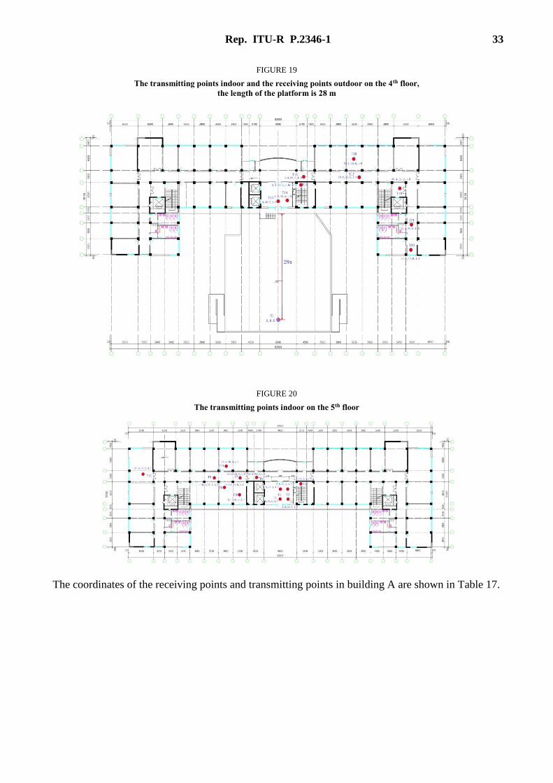
The receiving point located on the 4th floor platform outdoor, the main receiving point is labelled as
R1, marked as blue point in Fig. 19. Some transmitting points on the 4th floor indoor are marked as
red points in Fig. 19. Other transmitting points on the 5th floor indoor are marked as red points
shown in Fig. 20. Furthermore the receiving points and transmitting points are marked with
coordinate values, R1 is the coordinate origin.
FIGURE 18
The outdoor platform of the building A: The building scene from the receiving point, the thermal insulation layer is adding to
the exterior wall of the building A (Panoramic camera model,
Middle image of the building is slightly bent)
Rep. ITU-R P.2346-1 33
FIGURE 19
The transmitting points indoor and the receiving points outdoor on the 4th floor,
the length of the platform is 28 m
FIGURE 20
The transmitting points indoor on the 5th floor
The coordinates of the receiving points and transmitting points in building A are shown in Table 17.

34 Rep. ITU-R P.2346-1
TABLE 17
The coordinates of the receiving points and transmitting points in building A (unit: m)
Points x y z
R1 0 0 0
T1 0 29.6 4.7
T2 2.8 29.6 4.7
T3 2.8 33.4 4.7
T4 0.9 33.4 4.7
T5 5.1 34.2 4.7
T6 –6.8 35.3 4.7
T7 –10.6 35.5 4.7
T8 –18.1 35.4 4.7
T9 –14.9 32.6 4.7
T10 –11.7 31.4 4.7
T11 –15.4 38.3 4.7
T12 –37.9 36.9 4.7
T13 0 30.2 1.8
T14 2.8 30.5 1.8
T15 5.3 34.3 1.8
T16 5.9 35.5 1.8
T17 20.2 35.6 1.8
T18 19.1 40.6 1.8
T19 30.4 33.2 1.8
T20 33.7 17.8 1.8
T21 33.2 22.8 1.8
Some typical transmitting points’ pictures in building A are shown in Figs 21-23.

Rep. ITU-R P.2346-1 35
FIGURE 21
The transmitting point in the corridor of the building A
FIGURE 22
The transmitting point by the glass door of the building A

36 Rep. ITU-R P.2346-1
FIGURE 23
The transmitting point in the stair channel of the building A
9.1.2 Building B
Building B is a modern building combining toughened glass with reinforced concrete.
The toughened glass is laid in the wall which is known as a common toughened glass without metal
coat. Part of exterior wall is equipped with a brown ceramic tile. There is a parking lot outside the
building, the length of which is about 35 m. In order to avoid the influence of vehicle movement,
the method is:
– The test is taken at the weekend to make sure there are few vehicles and staff.
– Make sure the receiving antenna is away from the vehicle.
– The height of the receiving antenna is set to 2.3 m to ensure that the connection between the
transmitting antenna and the receiving antenna is not blocked by vehicles.
The main receiving point is R3, which is marked with blue point in Fig. 24, and the transmitting
points on the 1st floor are marked with red points in Fig. 25. The transmitting points on the 2nd floor
are marked with red points in Fig. 26. The transmitting points on the 3rd floor are marked with red
points in Fig. 27. The height of the transmitting antenna is 2.3 m and the height of the receiving
antenna is 2.3 m from the floors at that time.

Rep. ITU-R P.2346-1 37
FIGURE 24
Parking lot outside the building B: The building scene from the receiving point

38 Rep. ITU-R P.2346-1
FIGURE 25
The transmitting points indoor and the receiving point outdoor on the 1st floor in building B,
the length of the outdoor parking lot is 35 m

Rep. ITU-R P.2346-1 39
FIGURE 26
The transmitting points on the 2nd floor in building B
FIGURE 27
The transmitting points on the 3rd floor in building B

40 Rep. ITU-R P.2346-1
A coordinate system is formed with the R3 being a coordinate origin. The coordinates of the
transmitting points and receiving point are shown in Table 18.
TABLE 18
The coordinates of the receiving points and transmitting points in building B (unit: m)
Points x y z
R3 0.0 0.0 0.0
T23 0.0 –45.5 0.0
T24 –13.5 –45.5 0.0
T25 –13.5 –37.5 0.0
T26 –14.4 –60.8 0.0
T27 –11.6 –62.7 0.0
T28 7.8 –45.5 0.0
T29 14.8 –49.7 0.0
T30 23.9 –38.7 0.0
T31 13.8 –38.7 0.0
T32 22.1 –31.3 4.6
T33 13.0 –34.7 4.6
T34 11.9 –34.5 4.6
T35 22.1 –39.8 4.6
T36 21.2 –49.2 4.6
T37 14.8 –49.7 4.6
T38 7.8 –49.7 4.6
T39 10.9 –55.2 4.6
T40 20.8 –55.2 4.6
T41 –0.1 –49.5 4.6
T42 –11.7 –49.5 4.6
T43 –21.5 –49.5 4.6
T44 –22.6 –57.8 4.6
T45 –22.6 –41.6 4.6
T46 7.1 –35.5 7.8
T47 12.0 –44.1 7.8
T48 11.6 –55.2 7.8
T49 17.9 –55.2 7.8
T50 27.5 –55.3 7.8
T51 20.9 –57.0 7.8
T52 21.2 –49.2 7.8
T53 24.3 –43.6 7.8
T54 14.8 –49.2 7.8
Some typical transmitting points pictures in building B are shown in Figs 28-29.

Rep. ITU-R P.2346-1 41
FIGURE 28
The transmitting point in the lobby on the 1st floor in building B
(in transmitting point the receiving point can be seen through glass)
FIGURE 29
The transmitting point next to the elevator on the 2nd floor in building B

42 Rep. ITU-R P.2346-1
9.1.3 Building C
Building C is with reinforced concrete shear wall structure. The glass of windows of the building is
known as one-way transparent glass which has a good visibility from the inside to outside but a
poor visibility from the outside to the inside. In the measurement only one transmitting location is
selected, and the location is near the window, and 3 receiving locations are selected. From the
outdoor level, the transmitting antenna height is 3.3 m, the receiving antenna height is 2.3 m, the
horizontal distance from receiving point outdoor to transmitting point indoor is 9.65 m, 17.65 m and
29.65 m.
9.2 Test methodology
In building A and B, 11 frequency points are selected in 3.4 GHz to 3.6 GHz frequency band during
the test, which are: 3 401 MHz, 3 421 MHz, 3 441 MHz, 3 461 MHz, 3 481 MHz, 3 501 MHz,
3 521 MHz, 3 541 MHz, 3 561 MHz, 3 581 MHz, 3 601 MHz.
In building C, 3 frequency points are selected: 3 401 MHz, 3 501 MHz, 3 599 MHz.
9.2.1 Measuring system and instrument
The devices of measuring system are shown in Table 19.
TABLE 19
The antenna selection consideration
Transmitting antenna Omni-directional vertical polarization antenna
Receiving antenna • In building A and B: Omni-directional vertical polarization antenna.
• In building C: horn antenna with vertical polarization
Transmitter Agilent E8267D signal generator
RF power amplifier The output power in the test is set to 33 dBm
Receiver Agilent N9030A signal analyzer
We have developed an automatic program in order to control instruments and record test data by
LAN. In each location and frequency points, 500 continuous reading are obtained which will cost
about 8 ~10 seconds.
9.2.2 Calculation method of building entry loss
The free space loss can be calculated as:
𝐿𝑓 = 32.45 + 20 lg 𝑑(𝑚) + 20 lg 𝑓(𝐺𝐻𝑧) (3)
where d is defined in Fig. 30. f is carrier frequency (GHz). Set transmitted power be Pt (dBm) and
received power be Pr (dBm), the building entry loss is expressed as EL , transmitting antenna gain
and receiving antenna gain in transmission path are expressed as tG and rG , relatively.

Rep. ITU-R P.2346-1 43
FIGURE 30
The location relationship between the receiving antenna and the transmitting antenna
TxAntenna
RxAntennad
EL RG
TG
rP
tP
Then we can get equation (4).
𝑃𝑡(𝑑𝐵𝑚) + (𝐺𝑡 − 𝐿𝑓 − 𝐿𝐸 + 𝐺𝑟) = 𝑃𝑟(𝑑𝐵𝑚) (4)
And then the entry loss can be deduced from equation (5).
𝐿𝐸 = (𝑃𝑡(𝑑𝐵𝑚) − 𝑃𝑟(𝑑𝐵𝑚)) − 𝐿𝑓 + (𝐺𝑡 + 𝐺𝑟) (5)
The omni-directional antenna used in the test is similar to half wave dipole antenna whose gain is
2.15 dB, and the normalized directivity function of electric field of half-wave dipole antenna is
expressed as equation (6).
𝐹(θ) = 𝑠𝑖𝑛θ (6)
Where θ is defined in Fig. 29. From equation (6) we can get equation (7).
𝐺𝑡 + 𝐺𝑟 = 4.3 + 10 lg([𝐹(θ)]4) = 4.3 + 10 lg(sin4θ) (7)
In the scenario of building C, for horn antenna is used as receiving antenna, so the receiving
antenna gain is properly considered in calculation.
9.3 Measurement results
9.3.1 Measurement results and analysis of building A scenario
After processing the original test data the entry loss of building A can be obtained. Figure 31 shows
an example of curve of readings in time domain and median value.

44 Rep. ITU-R P.2346-1
FIGURE 31
Measurement of building entry loss: readings in time domain and median value
The median values of building entry loss measured above are shown in Table 20. The categories of
all links from transmitters and receivers can be separated as four types:
– Category0: Outer-wall with one-way transparent glass
– Category1: Outer-wall+1 inner-wall
– Category2: Outer-wall+2 inner-wall
– Category3: Outer-wall+ elevator.
TABLE 20
The median value of entry loss (building A, unit: dB)
Frequency
(MHz) 3 401 3 421 3 441 3 461 3 481 3 501 3 521 3 541 3 561 3 581 3 601 Category
Tx 1 27.3 20.2 36.9 29.5 28.7 32.1 37.7 24.5 28.4 45.0 38.5 0
Tx 2 20.0 19.5 19.7 19.9 22.1 29.1 16.1 20.7 18.1 17.6 28.0 0
Tx 3 21.2 25.8 22.3 21.1 25.0 22.9 27.4 25.1 23.8 23.4 28.1 0
Tx 4 34.3 26.7 24.4 25.7 23.1 26.8 25.9 27.6 22.0 24.0 27.4 0
Tx 5 46.3 45.1 56.5 41.4 40.3 44.2 45.1 36.6 37.9 41.3 42.9 1
Tx 6 44.5 40.6 38.3 42.0 43.0 37.7 43.2 41.2 47.0 49.7 56.6 3
Tx 7 42.6 44.4 49.2 44.7 71.3 44.1 41.0 44.2 42.7 39.9 39.0 3
Tx 8 39.1 45.8 45.7 42.8 43.3 46.5 48.0 49.0 51.4 53.6 53.0 1
Tx 9 27.6 36.1 26.5 21.8 36.7 37.2 20.1 31.8 32.9 24.1 31.8 0
Tx 10 19.2 24.8 27.4 25.8 26.1 42.1 30.2 26.9 23.0 24.2 29.8 0
0 1 2 3 4 5 6 7 835
40
45
50
(a) Time (s)
Build
ing E
ntr
y L
oss (
dB
)Building A. Entry Loss: Rx1,Tx20,V
t~V
r,3501MHz
Measured
Median value
36 38 40 42 44 46 480
0.2
0.4
0.6
0.8
(b) Entry loss distribution scale (dB)
Pro
babili
ty d
ensity

Rep. ITU-R P.2346-1 45
TABLE 20 (end)
Frequency
(MHz) 3 401 3 421 3 441 3 461 3 481 3 501 3 521 3 541 3 561 3 581 3 601 Category
Tx 11 51.9 57.7 65.4 60.2 53.0 64.3 62.9 63.9 59.7 56.3 51.9 2
Tx 12 60.3 53.6 63.0 56.2 54.1 51.1 51.1 55.1 55.4 57.4 58.4 2
Tx 13 27.1 34.5 33.3 34.9 50.2 28.7 29.0 36.7 32.1 39.2 40.9 0
Tx 14 40.2 35.7 38.1 30.2 26.4 32.4 28.1 33.3 35.4 40.9 30.1 0
Tx 15 53.0 50.7 55.5 49.1 41.6 44.3 57.5 46.7 66.3 56.6 53.1 3
Tx 16 50.5 53.1 60.3 55.6 46.9 50.8 47.2 52.5 57.0 69.0 57.1 2
Tx 17 51.9 52.1 55.5 61.1 44.1 52.7 43.5 50.0 42.1 46.3 49.8 2
Tx 18 60.0 66.2 76.1 68.9 66.8 75.0 69.9 74.0 65.8 70.6 61.7 2
Tx 19 58.3 63.5 64.2 58.3 65.0 66.5 73.2 61.5 60.9 64.1 64.6 2
Tx 20 31.8 33.7 33.7 33.4 32.5 40.5 45.3 43.4 35.3 36.9 33.7 1
Tx 21 43.3 54.5 52.8 50.9 55.2 47.9 59.9 52.6 44.2 50.8 43.2 1
Through analysis of median values of building entry loss (data in Table 20) at each frequency on
each transmitter, we can get the CDF, as shown in Fig. 32. And, the mean of data in Table 18 is
42.8 dB and standard deviation is 14.3 dB.
FIGURE 32
Cumulative distribution function of median values of each Tx at each frequency
10 20 30 40 50 60 70 800
10
20
30
40
50
60
70
80
90
100
CD
F (
%)
Building Entry Loss (dB)
CDF of median value for entry loss, Building A
20.8dB,5%
27.7dB,20%
43dB,50%

46 Rep. ITU-R P.2346-1
9.3.2 Measurement results and analysis of building B scenario
After processing the original test data the entry loss of building B can be obtained. The median
value of the entry loss measurement above is shown in Table 21. The categories of all links from
transmitters to receivers can be separated as four types:
– Category0: Outer-wall with glass
– Category1: Outer-wall+1 inner-wall
– Category2: Outer-wall+2 inner-wall
– Category1: Outer-wall+ elevator.
TABLE 21
The median value of the entry loss (building B, unit: dB)
Frequency
(MHz) 3 401 3 421 3 441 3 461 3 481 3 501 3 521 3 541 3 561 3 581 3 601 Category
Tx 23 16.9 8.1 9.6 4.1 9.6 13.5 11.5 5.9 12.6 12.5 18.5 0
Tx 24 22.0 12.6 8.2 15.9 21.0 20.3 13.0 15.0 13.0 22.6 19.4 0
Tx 25 16.1 10.5 21.0 10.5 12.7 13.0 26.6 9.4 21.8 18.8 13.2 0
Tx 26 9.6 12.7 11.2 12.1 22.1 10.8 11.4 14.2 16.0 16.4 6.6 0
Tx 27 16.6 19.5 15.8 23.7 36.7 22.0 14.5 18.9 15.3 16.5 12.0 0
Tx 28 11.3 19.6 10.8 12.2 20.8 21.8 22.9 11.7 19.3 12.2 8.3 0
Tx 29 25.9 22.3 31.9 26.6 29.7 25.1 33.5 22.6 22.0 21.6 24.4 3
Tx 30 20.9 18.3 25.1 18.2 20.4 19.5 19.2 20.5 22.9 32.0 24.7 1
Tx 31 20.4 15.7 12.9 17.8 25.4 13.3 30.7 14.5 20.3 24.6 17.5 0
Tx 32 41.7 36.2 38.4 29.9 47.2 38.2 40.5 38.9 36.2 40.3 35.3 0
Tx 33 36.1 31.3 36.1 22.0 33.6 42.1 38.8 33.4 26.4 26.9 29.4 0
Tx 34 19.9 25.6 31.5 33.5 24.6 23.8 27.4 26.8 36.6 30.7 26.0 0
Tx 35 22.7 27.8 24.4 26.3 34.1 29.1 28.7 21.7 21.3 25.2 24.9 1
Tx 36 40.9 42.3 33.6 45.3 32.0 33.1 41.3 37.8 33.1 47.8 32.5 2
Tx 37 30.1 48.4 46.6 35.1 38.4 40.4 40.0 32.7 41.7 39.1 31.6 2
Tx 38 22.7 17.6 25.3 20.4 16.0 30.1 21.1 24.8 17.7 25.6 20.9 0
Tx 39 34.9 39.7 36.5 31.5 34.0 37.4 36.6 32.0 37.3 34.5 36.3 3
Tx 40 45.3 38.6 35.0 37.5 48.4 43.7 39.2 44.3 39.2 40.9 42.5 3
Tx 41 14.4 21.4 17.8 17.6 20.4 22.2 22.6 16.1 22.8 21.3 26.1 0
Tx 42 18.3 19.4 18.7 16.4 21.6 20.0 33.1 25.8 19.4 23.4 21.8 0
Tx 43 32.9 33.3 30.4 36.5 42.6 30.6 37.9 34.3 32.5 36.3 39.2 1
Tx 44 48.1 35.6 39.1 53.6 43.8 37.0 48.5 42.8 53.8 41.5 35.2 2
Tx 45 30.7 35.9 32.4 47.1 33.7 38.0 31.6 37.6 26.7 36.8 29.6 1
Tx 46 13.4 16.3 32.5 17.2 25.6 19.5 17.4 23.7 20.5 33.4 22.5 0
Tx 47 26.2 29.5 34.8 33.4 37.0 31.9 30.8 47.7 25.4 29.2 35.3 1
Tx 48 39.4 53.2 49.3 43.5 50.6 44.1 48.1 51.2 53.8 48.3 63.0 3
Tx 49 61.2 48.4 60.8 46.1 56.0 57.8 63.2 57.1 57.8 51.0 60.8 3
Tx 50 55.4 58.9 61.1 52.9 52.5 59.7 55.0 53.2 63.7 59.8 51.1 3

Rep. ITU-R P.2346-1 47
TABLE 21 (end)
Frequency
(MHz) 3 401 3 421 3 441 3 461 3 481 3 501 3 521 3 541 3 561 3 581 3 601 Category
Tx 51 72.9 64.2 79.9 56.9 58.8 69.5 68.8 64.4 57.9 60.4 59.9 3
Tx 52 49.2 63.1 49.3 57.5 60.9 49.0 60.0 59.3 50.2 55.6 62.9 2
Tx 53 41.5 43.8 42.4 44.5 57.8 46.7 42.4 43.7 35.7 47.7 45.8 2
Tx 54 58.0 70.4 45.5 50.9 53.6 48.0 55.4 48.2 50.2 53.3 56.9 2
Through analysis of median values of building entry loss (data in Table 21) at each frequency on
each transmitter, we can get the CDF, as shown in Fig. 33. And the mean of data in Table 19 is
32.8 dB and standard deviation is 15.3 dB.
FIGURE 33
Cumulative distribution function of median value of each Tx at each frequency
0 10 20 30 40 50 60 70 800
10
20
30
40
50
60
70
80
90
100
CD
F (
%)
Building Entry Loss (dB)
CDF of median value for entry loss, Building B
12.9dB,5%
21.8dB,20%
37dB,50%

48 Rep. ITU-R P.2346-1
9.3.3 Measurement results and analysis of building C scenario
After processing the original test data the entry loss of building C can be obtained. The median
value of the entry loss measurement above is shown in Table 22.
TABLE 22
The median value of the entry loss, One Tx vs 3 Rx (Building C, unit: dB)
Frequency
(MHz) 3 401 3 501 3 599 Category
Rx 4 21.5 15.0 15.7 Outer wall with
glass
Rx 5 18.4 22.3 20.9 Outer wall with
glass
Rx 6 18.5 19.4 22.5 Outer wall with
glass
Through analysis of median values of building entry loss (data in Table 22) at each frequency on
each Rx, we can get the CDF, as shown in Fig. 34. And, the mean of data in Table 20 is 19.4 dB
and standard deviation is 2.7 dB.
FIGURE 34
Cumulative distribution function of median value of each Rx at each frequency
14 15 16 17 18 19 20 21 22 230
10
20
30
40
50
60
70
80
90
100
CD
F (
%)
Building Entry Loss (dB)
CDF of median value for entry loss, Building C
16.1dB,20%
18.1dB,50%
21.4dB,80%

Rep. ITU-R P.2346-1 49
10 Building entry loss measurement at 3.5 GHz in UK
10.1 UK measurements
A limited campaign of measurements has been undertaken to gather 3.5 GHz entry loss data for UK
buildings. The intention of this limited campaign was to inform discussions of BEL modelling
within SG 3 and to develop and refine measurement methods. If the results are considered useful,
it would be simple to extend the measurements, both within the UK and in other regions.
10.2 Methodology
The methodology adopted for the 3.5 GHz measurements closely follows that used in earlier UK
studies (see 3J/90). A portable, handheld, transmitter is used to explore the building under test, with
signals received at a transportable (vehicle-based) terminal located some tens of metres from the
building (but in LoS). Figure 35 shows the arrangement.
FIGURE 35
Experimental arrangement
The pathloss measured from within the building is compared with that measured from outside the
building, close to the wall facing the receiver. The ‘Building Entry Loss’ is then defined as the
difference between the median values of the two distributions.
Given the enormous variation in entry loss seen at different points throughout a typical building
(often around 30 dB), the measurements are broken down on a room-by-room basis. This seems to
be the smallest degree of discretisation that is useful in practice; rooms may be characterised as, e.g.
‘first-floor, away from receiver’ or ‘ground-floor, facing receiver’. To attempt to define positions
within rooms would rapidly become very complicated and building-specific and would be unlikely
to aid statistical analysis.
A separate results file is recorded for each room in the building; within each room, the engineer will
walk slowly around a semi-random route that explores the entire floor-area. It has been found that
this method gives results repeatable to within about 1 dB.
An important point is that the intention is that the ‘outdoor reference’ measurements are made at the
same height as the indoor measurements. This allows the modelling of building entry loss to be
decoupled from the modelling of other local environmental effects, such as clutter loss due to
surrounding buildings. It should be noted that this approach is not always followed in some of the
studies reported in the literature.

50 Rep. ITU-R P.2346-1
In the ideal case, the receiver would be located sufficiently far from the building to ensure both a
plane wavefront at the exterior wall and that the difference in free-space pathloss throughout the
building is negligible. In practice, the latter may be up to 6 dB and needs to be corrected for in post-
processing.
10.2.1 Hardware
The test source for the measurements is a small 2W transmitter operating at around 3.5 GHz. The
transmitter feeds a handheld co-linear (omnidirectional) antenna, radiating an unmodulated carrier.
The vehicle-mounted receive system consists of a flat-plate antenna mounted on an extensible mast,
feeding a Rohde & Schwarz FSP-13 spectrum analyser interfaced to a PC for data logging.
10.2.2 Software
The logging software recorded the received signal at a rate (1/80 ms) sufficient to capture the
fast-fading (Rayleigh) statistics of the path. This fast fading is filtered from the results reported
below, but could be explicitly included in the post-processing if required. Systematic analysis of
this data would be difficult, however, as the speed with which the transmitter moves is not constant.
10.3 Test locations
Four test locations have been used in this brief campaign, comprising a small residential building,
two large retail ‘superstores’ and a small office building. Measurements in a large modern office
block are also planned but have not been completed at the time of writing.
In all cases, a clear LoS was available between the outdoor terminal and an exterior wall of the
building under test.
10.3.1 Terraced house
This terraced family home (built in 1880) is of traditional brick construction, and has two rooms on
the ground floor, three on the first floor and one attic room in the roof-space.
FIGURE 36
Terraced house
The receiver, in this instance, was not mounted in the vehicle but on a tripod in the garden behind
the house, at a range of 13.5 m from the exterior wall.

Rep. ITU-R P.2346-1 51
10.3.2 Small office
A small office building of traditional brick constriction (built circa 1980) was measured with the
receiver vehicle in two locations, to the front and rear of the building. The accommodation is on
three floors.
FIGURE 37
Small office (Google Earth)
The measurements were made at ranges of 40 m (front) and 27 m (rear). The receiver locations and
the building under test are shown in the plan view below.
FIGURE 38
Plan view of small office showing receiver locations (Google Earth)

52 Rep. ITU-R P.2346-1
10.3.3 Retail buildings
Measurements were made in two retail buildings, both of steel-frame, brick clad construction and
both incorporating a large amount of metalwork in the interior fittings. The first, ‘Retail A’ was
a technology store occupying an area of 40 m × 40 m, with the receiver located at 35 m distance.
Measurements were made throughout the open-plan store, logged in 9 separate files representing
paths in the front, middle and back of the store and the right, middle and left sides of the building
(see Fig. 39, left).
The ‘Retail B’ building (a food supermarket) is significantly larger, and measurements were made
in a 20 m × 40 m subset of the floor area, as shown in Fig. 39, right). Two receiver locations were
used in this case, one at around 15° to the normal from the building and the other at around 40°. In
both cases the range was around 90 m.
FIGURE 39
Measurement plans – ‘Retail A’ on left, ‘Retail B’ on right (Google Earth)
Figure 40 shows a view of ‘Retail B’ from the antenna3 height at the second receiver location.
3 The UHF log-periodic antenna seen in the picture is not the measurement antenna.

Rep. ITU-R P.2346-1 53
FIGURE 40
View of ‘Retail B’ building
10.4 Results
10.4.1 Building entry loss
In line with the definitions given in Recommendation ITU-R P.2040, BEL is taken to be the
difference between the median field measured immediately outside the building and that measured
within each room or subdivision of the building.
The BEL can be quickly estimated by inspecting the cumulative distributions of the power recorded
at the outdoor receiver, as shown in Fig. 41, and comparing the indoor values with the outdoor
reference at the 0.5 probability point.
FIGURE 41
Summary results for ‘Retail B’ measurements
This figure shows that, as might be expected, the BEL increases (by 8-10 dB) as a function of depth
within the building4,5. The loss to the ‘outdoor reference’ is almost identical from the two receiver
4 The colour-coding of the traces follows that of the measurement areas in Fig. 39 (right).

54 Rep. ITU-R P.2346-1
locations, but it is interesting to note that the BEL values are greater for the more oblique ‘RX2’
measurements. This is in line with the Fresnel expressions for transmission loss through a plane
surface at different angles, though the effect is surprisingly clear and may equally be due to other
effects, such as diffraction loss from clutter within the store.
The results from the ‘Retail A’ building (Fig. 42) are very different in character, with smaller values
of loss (as might be expected for a smaller, less cluttered, store). Most interesting, however, is the
fact that there is very little dependence of BEL on penetration depth – possibly due to high levels of
scattered energy within the building.
FIGURE 42
Summary results for ‘Retail A’ measurements
The repeatability of measurements is indicated in Fig. 43, which shows two independent sets of
measurements for a single sub-section of the ‘Retail A’ building.
FIGURE 43
Showing repeatability of measurement
5 Note that BEL in the present definition includes both losses through the outer wall and additional losses
within the building.

Rep. ITU-R P.2346-1 55
10.4.2 BEL Variability
Characterising the variability of pathloss into or out of buildings is a non-trivial problem. In the
present context, we have defined variability to exclude multipath (selective fading) effects in line
with the ITU-R definition of outdoor ‘location variability’. This has the advantage of decoupling the
statistics from consideration of radio system bandwidth, but imposes a requirement to undertake
appropriate post-processing of the measured data.
As noted above, the simple nature of the present experimental arrangement6, with data gathered at
regular time intervals, but the terminal moving at arbitrary (walking) speed, precludes a very formal
approach to such post-processing. For the results reported here, a 4-point moving average was
applied to the data, which appears sufficient to remove the majority of selective fading while
preserving the flat fading due to clutter and other effects.
With this averaging applied, the measured data is found to be reasonably fitted7 by a lognormal
distribution, as shown in the figures below, which are normalised to the median value. Given the
current paucity of data, and the occasionally poor fit to the distribution tails (such as in Fig. 44a and
c), it is suggested that BEL statistics should only be modelled between decile points.
FIGURE 44
Sample loss distributions
6 Such a simple approach is probably pragmatically necessary, to allow large amounts of data to be
gathered rapidly.
7 Although some skewing is always evident at the low-loss tail of the distribution and occasionally at both
tails.
-15 -10 -5 0 5 10
0.001
0.003
0.01 0.02
0.05
0.10
0.25
0.50
0.75
0.90
0.95
0.98 0.99
0.997
0.999
Data
Pro
babili
ty
Normal Probability Plot
-12 -10 -8 -6 -4 -2 0 2 4 6 8
0.001
0.003
0.01 0.02
0.05
0.10
0.25
0.50
0.75
0.90
0.95
0.98 0.99
0.997
0.999
Data
Pro
babili
ty
Normal Probability Plot

56 Rep. ITU-R P.2346-1
a: ‘Small office’ (Gnd floor kitchen, SD = 4.9 dB) b: ’Retail B’ (Back), SD = 3.7 dB)
c: ‘House’ (study, SD = 5.5 dB) d: ’Retail A’ (mid), SD = 4.4 dB)
11 Building entry loss measurements at 28 GHz
11.1 Scenario
The measurement scenario is shown in Fig. 44. The outdoor antenna was mounted on the roof of
a parking garage 70 metres from the office, marked as point O in white, and the indoor antenna was
mounted on a tripod on the third floor of an office building, marked yellow in Fig. 45.
FIGURE 45
Configuration of the antennas
The office has both standard and coated window glass as indicated in Fig. 46. The indoor distance
between the walls with standard glass windows is 17 metres. The office landscape was empty apart
from interior walls indicated in Fig. 46, and no people were accessing the area during the
measurements. The weather-controlled textile outdoor blinds were not down during the first two
measurements, but they were down occasionally during the long term measurement.
-15 -10 -5 0 5 10 15
0.001
0.003
0.01 0.02
0.05
0.10
0.25
0.50
0.75
0.90
0.95
0.98 0.99
0.997
0.999
Data
Pro
babili
ty
Normal Probability Plot
-15 -10 -5 0 5 10
0.001
0.003
0.01 0.02
0.05
0.10
0.25
0.50
0.75
0.90
0.95
0.98 0.99
0.997
0.999
Data
Pro
babili
ty
Normal Probability Plot

Rep. ITU-R P.2346-1 57
FIGURE 46
Drawing of the office landscape with type of glass marked, the black dot marks the spot for the long-term measurement. The
distance between the walls with standard glass windows is 17 metres
11.2 Experimental Set-up
The radio units used as transmitters and receivers in the measurements are commercially-available,
all-outdoor single-carrier frequency division duplex (FDD) radio link units, operating in the 28 GHz
band. They have a channel bandwidth of up to 50 MHz (56 MHz channel spacing) and modulation
formats between 4 and 512 QAM, giving throughput between 94 and 406 Mbit/s at 50 MHz
bandwidth. Adaptive modulation mode was enabled on the radios, which means that the modulation
format depends on the mean square error detected by the radio, which in absence of additional
interference can be referred to a threshold in received power.
At the indoor unit, a highly directive integrated antenna was used for all measurements. This
antenna is a parabolic dish with diameter 0.24 m, 34 dBi gain, half-power beamwidth (HPBW) of
3.3 degrees, side-lobe level (SLL) below –20 dB and –30 dB at about 5 and 20 degrees,
respectively. The polarization of the antennas can be set to vertical or horizontal, and the cross-
polarization discrimination (XPD) is better than 30 dB within two times the HPBW. The antenna
was mounted 2 metres above floor level. At the outdoor unit, both the integrated 0.24 m antenna
and a vertically-polarized wide-beam slot array antenna were used in two separate measurement
setups. The wide-beam antenna has a gain of 22 dBi, a HPBW of 4.3 degrees in elevation, and
about 60 degrees in azimuth. The XPD is better than 25 dB within the main beam.
The angular distributions at the indoor locations were determined by rotating the indoor antenna in
the azimuth domain while continuously measuring the received power. This was done initially “by
hand,” but in a second campaign by using a motorized rotator to find the direction-of-arrival (DOA)
to the strongest multipath components (MPCs). The set-up used for the second measurement
campaign with the wide-beam outdoor antenna was also used for the long-term measurements.
For the long-term measurements the indoor antenna was aligned for maximum received power.
The output power was always set to have an operating microwave link connection between the
radios, though the transmitted power never exceeded +18 dBm. For the long-term measurements,
an attempt was made to keep the power levels as realistic as possible, lowering the transmitted
power of the indoor unit to minimize the regulated safety zone around the antenna. The transmitted
power from the outdoor radio was +18 dBm on the roof and the indoor unit transmitted at –10 dBm.

58 Rep. ITU-R P.2346-1
11.3 Data collection/analysis
The transmitted and received powers of both radios, together with the capacity of the link in both
directions, were collected during all measurements. The DOA angle of the maximum received
power was also noted. To study the long-term stability of a potential radio link setup, a four-day
measurement was conducted, with data collection every 30 seconds.
The excess loss in this paper is defined as the increase in loss relative to a measured reference LoS
level at the indoor window location A, at 70 m LoS distance (see Fig. 47), with the window open.
FIGURE 47
Attenuation for the first scenario with narrow-beam antenna on both sides, with vertical polarization (left) and horizontal
polarization (right). See Table 23 for the colour legend
TABLE 23
Colour legend used in Figs 47 and 48
Colour Excess loss
3-10 dB
11-20 dB
21-30 dB
31-40 dB
41-50 dB
51-60 dB
11.4 Results
The measurement results are presented in Figs 47-49. At every measured point, an operating
microwave link connection was established with a modulation format between 4 and 512 QAM.
The capacity of the microwave link was in agreement with the predicted capacity for the actually
received power and thus the link was usually not degraded due to multipath. At a couple of points
there was evidence of frequency-selective fading, as the received powers differed between the up-
and down-link directions. This was due to the separation of frequency in the FDD channel
(1 008 MHz separation at 28 GHz). The indoor radio was in that case moved so that the received
power in both directions became equal; the movement was less than 10 cm. Minor
frequency-selective fading was expected, as the path differences for possible multipaths were small.
Figure 47 visualizes the excess loss for horizontal and vertical polarization when using a narrow
antenna beam also at the outdoor unit. The reason for the steep increase in excess loss when moving
backwards into the office, point A to C, is because the actual LoS path becomes partially blocked

Rep. ITU-R P.2346-1 59
by the concrete pillars between the windows. From the measurement points further into the
building, point D to F, the waves can either propagate through the interior wall or diffract/reflect
around the interior cubical. Multiple MPCs with similar strengths were present.
Figure 48 shows the excess loss for vertical polarization with a sector antenna at the outdoor unit.
The reason for the variation in excess loss along the corridor is due to the concrete pillars, as
mentioned earlier, blocking the LoS path.
FIGURE 48
Attenuation in scenario two, with wide-beam antenna
at the outdoor site. See Table 23 for colour legend
Figure 49 shows the received power and capacity from a long-term measurement during four days.
The long-term measurement showed stable throughput and received power levels. The decrease in
received power, occurring every afternoon, was due to outdoor sun blinds going down
automatically to cover the windows. In this scenario, any major time-dependent changes of the
channel were not expected, as no person had access to the office landscape during the
measurements and the outdoor weather during this period was without any precipitation.
The difference in received power between the outdoor and indoor radio is due to the 28 dB
difference in transmitted power mentioned earlier. The capacity of the links was 406/285 Mbit/s in
down-/up-link, which correlates to a modulation format of 512/64 QAM. The up- and down-link
radios are independent and can send data in different modulation formats. The modulation formats,
as mentioned earlier, depend on the mean square error which, if no interference is present, is
directly dependent on the received power. The capacities measured are in good agreement with the
modulation format expected for the measured received power, indicating no degradation due to
interference/multipath.
FIGURE 49
Received power and throughput over 4 days; the difference in received power is due to
difference in transmitted power; the indoor unit transmitted 28 dB lower power

60 Rep. ITU-R P.2346-1
A loss of about 3-5 dB was measured in the standard glass window and about 30 dB in the coated
window, which is in good agreement with other8 observations.
At the indoor unit there was usually more than one incoming direction of waves. The attenuation in
Figs 47 and 48 refers to the strongest path. If a LoS path was available, this was always the clearly
dominating path, but in most other cases power was received from more than one incoming
direction. Two examples of this are shown in Fig. 48. The lengths of the arrows indicate the linear
relation between the received power in different DOA directions (a doubly-long arrow corresponds
to 3 dB higher received power). The length of the arrows is normalized to the highest received
power at that measured point and is not related to the length of the arrows at the other location. As
can be seen at the top left point there is almost equal power from two directions. All waves seem to
reach the point after passing through the narrow passage between the indoor cubicles, either through
multiple reflection or diffraction. One path obviously also includes a reflection from the windows
behind the measurement point. For the lower right measurement point, the paths are somewhat more
difficult to explain. This case involves a concrete wall and an evacuation staircase with coated
glass, blocking the LoS, which the signal is not penetrating so easily. As can be seen, the strongest
path is propagating via a final diffraction on the edge of the blocking concrete wall in the proximity
of the antenna. Regarding its path before the diffraction, it is not clear if it is reflection/diffraction
on the concrete pillars between the windows or multiple reflections within the office space. Beyond
this strongest path, 6 paths reaching the measurement point by reflection were also measured. Since
these are about 10 dB below the strongest one, they are difficult to see in the picture.
11.5 Conclusion
The results show that attenuation/excess loss limits the coverage, rather than multipath interference.
In the scenario studied, coverage was obtained at all measured locations with a loss between 3 and
60 dB above the reference level at 70 m LoS distance. If all windows in the office had been of the
coated glass kind, then at least 20 dB higher excess loss would be expected and the coverage would
be significantly more limited. Thus, the deployment opportunities strongly depend on the specific
location and the kind of windows that are present.
It is concluded that the indoor environment at this location is not isolated from the outdoor cell.
Thus, at many locations it will be possible to provide, for example, a backhaul link between an
indoor wall-mounted high gain antenna and a similar outdoor antenna, even when the indoor excess
loss is extensive.
12 Measurements at 5.2 GHz
The experimental results shown in Table 24 were obtained at 5.2 GHz through an external building
wall made of brick and concrete with glass windows. The wall thickness was 60 cm and the
window-to-wall ratio was about 2:1.
8 Zhao, H., et al., “28 GHz Millimetre Wave Cellular Communication Measurements for Reflection and
Penetration Loss in and around Buildings in New York City”, Proc. IEEE International Conference on
Communications (ICC 2013), June 2013.

Rep. ITU-R P.2346-1 61
TABLE 24
Example of building entry loss
Frequency Office
Mean
Standard
deviation
5.2 GHz 12 dB 5 dB
Table 25 shows the results of measurements at 5.2 GHz through an external wall made of stone
blocks, at incident angles from 0° to 75°. The wall was 400 mm thick, with two layers of 100 mm
thick blocks and loose fill between. Particularly at larger incident angles, the loss due to the wall
was extremely sensitive to the position of the receiver, as evidenced by the large standard deviation.
TABLE 25
Loss due to stone block wall at various incident angles
Incident angle (degrees) 0 15 30 45 60 75
Loss due to wall (dB) 28 32 32 38 45 50
Standard deviation (dB) 4 3 3 5 6 5
13 Building Entry Loss from 5-32 GHz
13.1 Introduction
This section presents measurements of outdoor-to-indoor propagation from 5-32 GHz. For this
exercise three different buildings were measured. The first is a newer building (built in 2009) that is
similar in construction to a modern residential home in the United States. The second is an older
commercial office building (built in 1945). The last building is a very new commercial office
building built using modern “green” building techniques. These two buildings allow for the
measurement of propagation losses through both modern and older materials such as glass/windows
and exterior block and siding. The excess loss (with free space loss removed) for both buildings is
presented in this document.
13.2 Experimental Setup
The signals used during this experiment were continuous wave (CW) at 5, 12, 25.5 and 32 GHz.
The antennas used for both the transmitter and receiver were identical dual ridge horn antennas
(MVG Model Number: SH4000) with the following characteristics:

62 Rep. ITU-R P.2346-1
FIGURE 50
Picture of the antenna used for the experiment
TABLE 26
Transmit and receive antenna parameters
Antenna Gain 4.5-13 dBi (Frequency Dependent)
3 dB Beamwidth 80-40° (Frequency Dependent)
Gain Stability ±1 dB
The outdoor transmitter consisted of a signal generator (Anritsu MG3690C) connected to the dual
ridge horn antenna, with an optional amplifier that was not used for this experiment but could be
included for future measurements if necessitated by the expected free space loss. The receiver
consisted of an identical antenna connected to a spectrum analyzer (Agilent E4446A). Initially two
identical receivers were setup with the intent on simultaneously measuring the outdoor reference
and the indoor locations, as indicated by Recommendation ITU-R P.2040-1. However due to
observed coupling between the two receive antennas, it was decided that the outdoor and indoor
measurements would be conducted separately.

Rep. ITU-R P.2346-1 63
FIGURE 51
Block diagram of the receiver (left) and transmitter (right) used for the experiment
13.2.1 Building descriptions
The first building that was measured is a recently constructed building similar to a modern US
residential building. The building’s exterior is made up of vinyl siding followed by plywood
sheeting with metal studs with fiberglass insulation in-between covered by final layer of drywall.
The windows in the building are standard double pane low-emissivity windows used in most
modern US construction.
The second building is an older commercial office building. The exterior walls are composed of
10.2 cm of brick on top of 20.3 cm of concrete block followed by 2.5 cm furring strips and 1.9 cm
layer of plaster. The windows are older and made of double pane glazed glass with aluminium
frames.
The third building is a new building that was constructed with a focus on environmental factors,
e.g. a lot of recycled/energy efficient material and low E glass windows. There also is a reflective
thermal coating on the windows to help keep the building cool in the summer and warm in the
winter. This coating as well as the low E glass seems to have a large effect on the transmission of
signals into/out of the building, as will be shown in the results that follow.
FIGURE 52
Photograph of the front of Building 1 (left) and Building 2 (right) and Building 3 (bottom)
13.2.2 Testing Locations
For each test point the transmitter was positioned so that the signal had normal incidence onto the
face of the building. The receiver was then positioned in direct line of sight (LOS) at 0° azimuth
with reference to the transmitter. The height of the transmitter and receiver were matched to

64 Rep. ITU-R P.2346-1
eliminate any changes in the received signal level due gain deviations in the antenna patterns.
Figure 53 shows the locations of each antenna during the experiment for both the reference
measurement and the actual building measurement.
FIGURE 53
Depiction of experimental setup
FIGURE 54
Photos of the transmitter and receiver during testing
After the outdoor reference measurement was taken, the receiver was moved into the building and
positioned to again be a at 0° azimuth with reference to the transmitter and at the same height as
both the outdoor measurement and the transmitter. A laser transit system was used to match the
heights and to account for any changes in ground elevation. For each transmitter location the indoor
measurements were stepped linearly, moving farther away from the transmitter at each test point
taking care to ensure that the 0° azimuth with reference to the transmitter was maintained thought
the experiment.

Rep. ITU-R P.2346-1 65
FIGURE 55
Diagram showing how receiver was linearly stepped into building
When the rear of the building was reached the transmitter was repositioned to the next location and
the process was repeated. The transmitter was stepped across the face of the building to ensure that
there was always normal incidence on the building face and so that the transmitter and receiver
were always pointed boresight to reduce/eliminate signal level changes due to gain variations over
the beamwidth. The floor plans and the testing locations of each building are shown in Figs. 56-58.
The spatial density of points needs to be considered when conducting an experiment such as this.
The testing locations were chosen to be somewhat uniformly distributed and to ensure that all of the
unique aspects of the building were sampled (e.g. windows, doors, large wall sections, hallways,
etc.). For Building 1 the spatial density was 1 point per 5 square meters, for Building 2 it was 1
point per 14 square meters, and for Building 3 it was 1 point per 27 square meters. The points were
designated by defining an arbitrary origin at a location inside the building, then referencing all
spatial locations to that origin.
FIGURE 56
Floor plan and testing locations for Building 1

66 Rep. ITU-R P.2346-1
FIGURE 57
Floor plan and testing locations for Building 2
FIGURE 58
Floor plan and testing locations for Building 3

Rep. ITU-R P.2346-1 67
FIGURE 59
Photos of the interior testing points being laid out using tape measures to reference the defined origin
13.2.3 Data post processing
At each test point in the experiment a minimum of two minutes of data per frequency was collected
at 1 Hz. In post processing the temporal data at each test point was subjected to a trimmed average
by calculating the standard deviation (σ) of all the samples at a particular point and frequency then
removing any outliers (defined as values exceeding ±3σ) then averaging the remaining points. The
total number of outliers removed from the data set comprised less than 0.5% of the total samples
collected.
The building entry loss in this paper is defined as:
𝐵𝐸𝐿(𝑥, 𝑦) = 𝑃𝑟𝑒𝑓(𝑥, 𝑦, 𝑡0) − 𝑃𝑖𝑛𝑑𝑜𝑜𝑟(𝑥, 𝑦, 𝑡𝑛) − 𝐿𝐹𝑆(𝑥, 𝑦)
Where 𝐵𝐸𝐿 is the building entry loss, 𝑃𝑟𝑒𝑓 is the time averaged power received at the outdoor
reference location, 𝑃𝑖𝑛𝑑𝑜𝑜𝑟 is the received power at the indoor location and 𝐿𝐹𝑆 is the additional free
space loss that occurred from the signal traveling past the reference point and into the building.
13.3 Results
The following sections contain the results of the measured building loss from each building. The
results are analyzed and presented in several different ways, including: tabulated, visually with 2D
maps and statistically.
13.3.1 Tabulated Results
The tabulated measurements results are presented in Tables 27 to 29. From the data in Tables 27 to
29, it can be seen that the range of building loss seen is quite large depending on the position inside
the building. The minimum BEL seen was on the order of 1-2 dB with the maximum in excess of
50 dB. It is important to note that for each building the measurements were taken over the course of

68 Rep. ITU-R P.2346-1
a single evening and that during the time measurements were taken the temperatures deviation was
less than 6°C. Additionally, there was no precipitation during testing.
TABLE 27
Tabulated Building Loss Results for Building 1
Frequency
[GHz]
Minimum
[dB]
Mean
[dB]
Maximum
[dB]
Standard Deviation
[dB]
5 1 8.5 27 6.5
12 .5 9.5 23.5 5.5
25.5 3.5 14 32 6
32 2.5 17 40 7.5
TABLE 28
Tabulated Building Loss Results for Building 2
Frequency
[GHz]
Minimum
[dB]
Mean [dB] Maximum
[dB]
Standard Deviation
[dB]
5 1 13.5 32.5 9.5
12 1 14 30 9.5
25.5 1.5 17.5 52.5 15
32 2.5 14.5 45 14.5
TABLE 29
Tabulated Building Loss Results for Building 3
Frequency
[GHz]
Minimum
[dB]
Mean [dB] Maximum
[dB]
Standard Deviation
[dB]
5 11.5 29 53 12
12 16 31 51.5 11
25.5 13 35.5 69 14.5
32 20.5 38 58.5 12
It is important to note that for each building the measurements were taken over the course of a
single evening and that during the time measurements were taken the temperatures deviation was
less than 6°C. Additionally, there was no precipitation during testing.
It is also important to note that all of the buildings presented a multipath rich environment. This
created a substantial amount of variation in the received signal as a function of position. Multipath
has the potential to be both constructive and destructive. When considering any single spatial point,
the contribution of multipath should be taken into account, and therefore some of the minimum (and
maximum) values in the above tables are likely influenced by multipath. Additionally, the
reciprocal nature of the propagation path was not measured and therefore the measured building
entry losses shown in Tables 27 to 29 may not necessarily be equated to building exit losses.

Rep. ITU-R P.2346-1 69
13.3.2 Coverage maps
A visualization of the building entry loss seen inside the building is shown in Figs 60 to 62. These
figures were generated by taking the averaged data points and applying a 2D spline interpolation to
approximate what the building entry loss values would be throughout the entire building. High
levels of loss are expressed as warm colours (reds, yellows etc.) and lower levels of loss are cool
colours (greens, blues etc.).
FIGURE 60
Interpolated building entry loss map of Building 1

70 Rep. ITU-R P.2346-1
FIGURE 61
Interpolated building entry loss map of Building 2
FIGURE 62
Interpolated building entry loss map of Building 3

Rep. ITU-R P.2346-1 71
From these plots it appears that the measurement results are more uniform in Building 1. This is due
to the open nature of the building, as seen from the floor plan. Once inside building one the majority
of the area is contained inside one large “great room” with very few interior walls or furniture.
Conversely, Building 2 and 3 are subdivided into many offices and those offices are further divided
into individual cubicles each containing standard office furniture, desk, chairs, bookshelves, etc.
In both buildings there appeared to be a large amount of multipath as the signal diffracted/reflected
off the building interior. For the purpose of this experiment the receivers were kept pointed
boresight with the transmitter but a large amount of signal variation occurred with azimuth rotation.
This effect needs to be explored further to characterize the overall role of multipath in building
entry loss.
13.3.3 Distance dependency
The next three figures (Figs 63-65) show the relationship between the building entry loss and the
distance from the transmitter, keeping in mind the all of the free space loss has been removed.
There are four curves on each plot, corresponding to the four discrete frequencies that were tested.
The 5, 12, 25.5 and 32 GHz curves are the dark blue, green, red and light blue curves respectively.
FIGURE 63
Building entry loss as a function of distance into Building 1

72 Rep. ITU-R P.2346-1
FIGURE 64
Building entry loss as a function of distance into Building 2
FIGURE 65
Building entry loss as a function of distance into Building 3

Rep. ITU-R P.2346-1 73
From the above Figures, it can be seen that there is an increasing trend in building entry loss as a
function of distance inside of the building. This is due to the increase in different propagation
mediums encountered as the signal travels into the building, e.g. interior walls, furnishings. This
effect is more prevalent in Building 2 where the building had many interior walls and an abundance
of furnishings.
13.3.4 PDF Distributions
Next the probability density functions (PDFs) of the data sets are considered. The distributions
appear to be lognormal with the mean and standard deviation varying with frequency. Plotted
alongside the actual PDF results are simulated lognormal PDFs using the means and standard
deviations listed in Tables 27 and 28. The results from Building 1 more closely match the simulated
log normal PDFs, this is most likely due to the open nature of the building with very few interior
walls or furnishings. Additional data points for Buildings 2 and 3 could potentially enhance the PDF
results and give a more accurate indication as to the PDF distributions.
More buildings will need to be measured in order to expand upon and examine these trends in more
depth and confirm the conclusions about the distributions; but this information is promising for
future modelling purposes.
FIGURE 66
PDF Distributions of Building 1

74 Rep. ITU-R P.2346-1
FIGURE 67
PDF distributions of Building 2
FIGURE 68
PDF distributions of Building 3
0 5 10 15 20 25 30 35 400
0.1
0.2
0.3
0.4
0.5
0.6
0.7
0.8
0.9
15GHz PDF
Building Entry Loss [dB]
No
rma
lize
d P
erc
en
tag
e o
f O
ccu
ran
ce
0 5 10 15 20 25 30 35 400
0.1
0.2
0.3
0.4
0.5
0.6
0.7
0.8
0.9
112GHz PDF
Building Entry Loss [dB]
No
rma
lize
d P
erc
en
tag
e o
f O
ccu
ran
ce
0 5 10 15 20 25 30 35 400
0.1
0.2
0.3
0.4
0.5
0.6
0.7
0.8
0.9
125.5GHz PDF
Building Entry Loss [dB]
No
rma
lize
d P
erc
en
tag
e o
f O
ccu
ran
ce
0 5 10 15 20 25 30 35 400
0.1
0.2
0.3
0.4
0.5
0.6
0.7
0.8
0.9
132GHz PDF
Building Entry Loss [dB]
No
rma
lize
d P
erc
en
tag
e o
f O
ccu
ran
ce
0 5 10 15 20 25 30 35 40 45 500
0.2
0.4
0.6
0.8
1
5GHz PDF
Building Entry Loss [dB]
No
rma
lize
d P
erc
en
tag
e o
f O
ccu
ran
ce
0 5 10 15 20 25 30 35 40 45 500
0.2
0.4
0.6
0.8
1
12GHz PDF
Building Entry Loss [dB]
No
rma
lize
d P
erc
en
tag
e o
f O
ccu
ran
ce
0 5 10 15 20 25 30 35 40 45 500
0.2
0.4
0.6
0.8
1
25.5GHz PDF
Building Entry Loss [dB]
No
rma
lize
d P
erc
en
tag
e o
f O
ccu
ran
ce
0 5 10 15 20 25 30 35 40 45 500
0.2
0.4
0.6
0.8
1
32GHz PDF
Building Entry Loss [dB]
No
rma
lize
d P
erc
en
tag
e o
f O
ccu
ran
ce

Rep. ITU-R P.2346-1 75
13.3.5 CDF Distributions
Finally the cumulative distribution functions (CDFs) are examined. The CDFs show that 90% of the
time the loss contributed to the building was less than 26 dB for all frequencies in Building 1,
however the higher frequencies saw increased loss in Building 2 with 90% of the overall building
entry loss seen being less than 40 dB. Building 3 had the lowest minimum building entry loss seen
over 10 dB however 90% of the measurements were still less than 40 dB.
FIGURE 69
CDF of building entry loss for Building 1
Perc
enta
ge o
f D
ata
Set
That
Ex
cee
de
d B
EL V
alu
e

76 Rep. ITU-R P.2346-1
FIGURE 70
CDF of building entry loss for Building 2
FIGURE 71
CDF of building entry loss for Building 3
Per
centa
ge
of
Dat
a S
et T
hat
Ex
ceed
ed B
EL
Val
ue

Rep. ITU-R P.2346-1 77
13.4 Tables of Building Parameters
Recommendation ITU-R P.2040 recommends the completion of the following Tables to identify
pertinent details about the buildings testing and the measurements taken.
TABLE 30
Measurement parameters for Building 1
Frequency 5, 12, 25.5 and 32 GHz
Bandwidth of test signal 0 MHz
Surrounding environment Suburban
Line of sight to building? Yes
Averaging Temporal averaging at each test point
Penetration depth 1 = indoor terminal in room/space with
external wall facing outdoor terminal
Floor on which measurements made Ground floor = 0
Area within which samples taken 180.88 m2
Number of samples 42 spatial points with 100+ temporal samples
at each location
Reference 1 = measured median signal
Distance of outdoor terminal from building 3.3528 m
Elevation angle of path 0°
Minimum azimuth with respect to normal to building
face 0°
Maximum azimuth with respect to normal to building
face 0°
Width 15.2 m
Length 15.2 m
Height 7.6 m
Total number of floors 1
Thickness of exterior walls .152 m
Thickness of interior walls .152 m
Thickness of floors N/A
Proportion of building elevation area composed of
windows/apertures %
Window elements 2 = double
Window coating 0 = unknown
Metallic thermal insulation fitted? 0 = unknown
Floor material 3 = concrete
Primary Exterior wall material 5 = wooden
Secondary Exterior wall material 8 = metal
Internal walls 7 = Plasterboard (metal stud)
Roof materials 5 = wood with roofing felt

78 Rep. ITU-R P.2346-1
TABLE 31
Measurement parameters for Building 2
Frequency 5, 12, 25.5 and 32 GHz
Bandwidth of test signal 0 MHz
Surrounding environment Suburban
Line of sight to building? Yes
Averaging Temporal averaging at each test point
Penetration depth 1 = indoor terminal in room/space with
external wall facing outdoor terminal
Floor on which measurements made Ground floor = 0
Area within which samples taken 700 m2
Number of samples 50 spatial points with 100+ temporal samples
at each location
Reference 1 = measured median signal
Distance of outdoor terminal from building 15.8 m
Elevation angle of path 0°
Minimum azimuth with respect to normal to building
face 0°
Maximum azimuth with respect to normal to building
face 0°
Width 12.1 m
Length 60.9 m
Height 7.6 m
Total number of floors 2
Thickness of exterior walls .352 m
Thickness of interior walls .152 m
Thickness of floors N/A
Proportion of building elevation area composed of
windows/apertures %
Window elements 2 = double
Window coating 0 = unknown
Metallic thermal insulation fitted? 0 = unknown
Floor material 3 = concrete
Primary Exterior wall material 2 = brick
Secondary Exterior wall material 4 = lightweight block
Internal walls 7 = Plasterboard (metal stud)
Roof materials 9 = other

Rep. ITU-R P.2346-1 79
TABLE 32
Measurement parameters for Building 3
Frequency 5, 12, 25.5 and 32 GHz
Bandwidth of test signal 0 MHz
Surrounding environment Suburban
Line of sight to building? Yes
Averaging Temporal averaging at each test point
Penetration depth 1 = indoor terminal in room/space with
external wall facing outdoor terminal
Floor on which measurements made Ground floor = 0
Area within which samples taken 1400 m2
Number of samples 40 spatial points with 100+ temporal samples
at each location
Reference 1 = measured median signal
Distance of outdoor terminal from building 11.5 m
Elevation angle of path 0°
Minimum azimuth with respect to normal to building
face 0°
Maximum azimuth with respect to normal to building
face 0°
Width 12.1 m
Length 46 m
Height 18 m
Total number of floors 3
Thickness of exterior walls .352 m
Thickness of interior walls .152 m
Thickness of floors N/A
Proportion of building elevation area composed of
windows/apertures 80%
Window elements 2 = double
Window coating 9 = other
Metallic thermal insulation fitted? 0 = unknown
Floor material 3 = concrete
Primary Exterior wall material 7 = glass
Secondary Exterior wall material 8 = metal
Internal walls 7 = Plasterboard (metal stud)
Roof materials 9 = other
13.5 Conclusion
The characterization of building entry loss is not a trivial task to undertake. There are many
variables which must be isolated, such as free space loss, multipath, RF clutter, etc. This experiment
sought to eliminate as many variables as possible and focus only of the actual loss introduced by the

80 Rep. ITU-R P.2346-1
building itself. The results of this study have shown that building entry loss is dependent upon the
building which is being studied both in terms of its composition and its contents (interior walls,
furniture, etc.). Within the two buildings studied, building entry loss as low as 0.5 dB and in excess
of 50 dB was observed. However, even though the building results varied the PDF distributions of
both appear to be lognormal, these results will be expanded upon and examined in more depth when
additional buildings are completed.
14 Measurements at 3, 10 and 17 GHz
14.1 Measurement Campaign
This section presents a description of the measurement campaign from the considered scenarios to
the setup parameters and the employed procedure to perform the measurements.
14.1.1 Scenario Description
The measurement scenario, displayed in Fig. 72 and Fig. 73, describes the O2I propagation scenario
where the transmit antenna is located outside and mounted on top of a van (2.5 m above ground
level). The receiver (RX) was located inside a building (Orange Labs premises in Belfort, France) at
different location points where measurement data were collected. The location points refer to the
different offices and corridors inside the building. The environment around the RX positions
consisted of office and flat furniture in addition to the interior walls. The receive antenna height was
kept at mobile user level (1.5 m). The distance between the transmitter (TX) and the exterior walls
of the building was around 10 m.
FIGURE 72
Outdoor-to-Indoor Scenario. The TX is installed in the white measurement van and the RX is located
inside the building marked out by the 2-sided orange arrow

Rep. ITU-R P.2346-1 81
FIGURE 73
Building Map and Room Pictures. Each number i corresponds with an RX position Ri. a) Corridor,
b) Living Room, c) Small Office inside the Flat, d) Break Room, e) Large Office
R21LoS, R23LoS and R14LoS will correspond with the RX positions at R21, R23 and R14
respectively, when the windows are opened, i.e. when the TX and the RX are in LoS conditions.
14.1.2 Setup and Procedure
The measurement campaign was conducted using a wideband channel sounding system [6] to
characterize the propagation channel. The distance between the TX and the RX units was a few
meters (10 to 25 m). An arbitrary waveform generator (AWG) generated successive 8192-length
wideband sequences at 1 Gbps-rate with a 125 MHz channel bandwidth. The transmitted powers
ranged from 23 to 30 dBm approximately, according to the frequency.
Depending on the RX antenna radiation patterns, the conducted measurements can be classified into
two categories:
− Omnidirectional (Omni.) measurements: characterized by the use of omnidirectional RX
antennas.
− Directional (Dir.) measurements: with the use of directional RX antennas.
Table 33 recapitulates the different measurement setup parameters.

82 Rep. ITU-R P.2346-1
TABLE 33
Measurement Setup Parameters
Setup Parameters Omni. Dir.
3 GHz 10 GHz 17 GHz 17 GHz
Frequency bands (GHz) 3.6-3.725 10.5-10.625 17.3-17.425
Tx Sequences (8192-length, 1Gbps-rate)
Bandwidth 125 MHz
TX Power 23-30 dBm
RX Antenna gain (dBi) 1 dBi (Omni) 0 dBi (Omni) 0 dBi (Omni) 7 dBi
(Dir)*
TX antenna gain (dBi) 1 dBi (Omni) 0 dBi (Omni) 7 dBi (Dir)* 7 dBi
(Dir)*
TX and RX antenna Polarization Vertical
Antenna height TX: 2.5 m and RX: 1.5 m
(above ground level)
Tigger time 100 ms
(*) with 90° beam-width.
During the omnidirectional measurements, the RX antenna which was mounted on a rotating arm
describing a circular trajectory. The radius of the trajectory was 2λ at 3 GHz, 4λ and 6λ at 10 and
17 GHz respectively.
However for the directional measurements, the directional RX antenna was pointing towards
4 different directions with 90° angular step (antenna beam-width) partitioning the space in 4 sectors.
In each sector the antenna remained static while the data were being collected.
14.2 Data Processing
In this section, we describe the data processing and define channel metrics such as the building
penetration losses LO2I and the delay spread DS.
For the measurements performed with omnidirectional RX antennas at 3, 10 and 17 GHz, at a given
RX position, let hn(τm) be the propagation channel complex impulse response (CIR) of the nth
measurement snapshot and N the total number of measurement snapshots distributed along the
circular trajectory.
Similarly for the directional measurements at 17 GHz, we will note hn,k(τm) the channel CIR of the
nth measurement snapshot in the kth sector and K the total number of sectors.
The measured channel CIRs are generally impacted by noise which can lead to a biased estimation
of the penetration losses and the delay spread. The instantaneous dynamic range (difference
between the CIR peak value and the noise level) ranged from 20 to 40 dB. Therefore, a single
threshold of 20 dB was applied to all the CIRs allowing for a fair comparison between the different
frequencies and scenarios. For example for the nth measurement snapshot at a given RX position,
only channel CIR samples τ compliant to the condition (8) were considered.

Rep. ITU-R P.2346-1 83
20
max
10log10
2
n
n
h
h
(8)
For the omnidirectional measurements, the channel power delay profile (PDP) is given by (9):
N
n
nhN
PDP
1
21 (9)
with τ the relative delay.
Regarding the directional measurements, the averaging of the measurement snapshots is done in the
complex domain in order to remove the noise effects (10).
K
k
knk hN
h
1
,1
(10)
The PDP is then obtained by summing the power contributions of the K sectors (11).
K
k
khPDP
1
2 (11)
This synthesizing procedure is similar to the method presented in [14].
The channel attenuations (Apeak, Aav and Amax), expressed in dB, are defined as following:
Let τmax be the delay maximizing the PDP:
RXTX GGPDPA max10max log10 (12)
RXTXav GGPDPA
10log10 (13)
RXTXnpeak GGhnA
2max10log10 (14)
GTX and GRX are the TX and RX antenna gains respectively.
Amax and Apeak are defined to illustrate the LoS conditions and the multi-path fading phenomena and
noise effects. The parameter Aav is an important characteristic since it expresses the average
attenuation of the propagation channel.
The averaging procedure in (2) contributes to filter the small-scale fading effects caused by multiple
propagation paths. These multipath fading effects can be noticed in Fig. 74 where the behavior of
the channel peak-attenuation Apeak for a given RX position during the omnidirectional
measurements at 17 GHz is shown.

84 Rep. ITU-R P.2346-1
FIGURE 74
Peak-Attenuation Variation at 17 GHz (Omni.) for R32
However, in Fig. 75, the small variations of the channel peak-attenuation during the directional
measurements at 17 GHz are typical effects due the presence of noise. Hence the averaging in the
complex domain, performed in (10), is more suited to cancel out these effects.
FIGURE 75
Peak-Attenuation Variation at 17 GHz (Dir.) for A5
The dynamic range is also considerably improved as illustrated in Fig. 76 where it can be noticed
that the noise level is significantly lower in the directional case than in the omnidirectional one.
FIGURE 76
PDP (Dir. Vs Omni.) 17 GHz for R24
Figure 77 also shows the PDPs of the different sectors at a given RX position as well as the
resulting synthesized PDP as described previously. This is representative of the channel
characteristics assuming omnidirectional RX antennas.
0 50 100 150 200 250 300 350105
110
115
120
125
130
135
140
145
Measurement Snapshots
Am
plitu
de
(d
B)
Peak-Attenuation Variation
Average Value
0 100 200 300 400 500 600110
112
114
116
118
120
Measurement Snapshots
Am
plitu
de
(d
B)
Peak-Attenuation Variation
Average Value
3.8 3.9 4 4.1 4.2 4.3 4.4 4.5 4.6-70
-60
-50
-40
-30
-20
-10
0
Relative Delay Time (us)
No
rma
lize
d M
ag
nitu
de
(d
B)
Directional
Omnidirectional

Rep. ITU-R P.2346-1 85
FIGURE 77
PDPs from Dir. Measurements at 17 GHz for R7
We define the building penetration losses, LO2I (15), as an additional attenuation compared to the
theoretical free-space path loss (FSPL) LFS.
FSavIO LAL 2 (15)
where dfL cFS 1010 log20log205.147 .
LFS is expressed in dB, fc is the carrier frequency expressed in Hz and d the distance between TX
and RX in m.
This parameter LO2I takes into account the attenuation due to the penetration through external walls
and/or windows and also the losses caused by the elements present in the indoor propagation
environment.
Finally, we quantify in (16) the channel delay spread DS.
)(
)(2
PDP
PDP
DS
mean
(16)
where:
)(
)(
PDP
PDP
mean
14.3 Measurement results and analysis
14.3.1 Measurement validation (LoS cases)
In this section, we propose to determine the validity of the omnidirectional and directional
measurements by verifying how close the attenuation Amax is to the FSPL LFS in LoS conditions.
Generally, in LoS conditions, there is a main path corresponding to the signal LoS component.
Therefore, for the RX positions (R21LoS, R23LoS and R14LoS) considered as LoS cases, the
attenuation value Amax should be equal to LFS.
An up-sampling factor of 2 was applied to the channel CIRs in order to get a better estimation of
Amax (peak-detection).
3.2 3.3 3.4 3.5 3.6 3.7 3.8-80
-70
-60
-50
-40
-30
-20
-10
0
Relative Delay Time (us)
No
rma
lize
d M
ag
nitu
de
(d
B)
Sector #1
Sector #2
Sector #3
Sector #4
Synthesized PDP

86 Rep. ITU-R P.2346-1
We define ϵ as the gap between the two values of attenuation (ϵ = Amax − LFS) for the three RX
positions (R21LoS, R23LoS and R14LoS). The computed values of attenuation for the three carrier
frequencies are summarized in Table 34.
TABLE 34
Measurement Agreement with Free-Space Law
ϵ[dB] Omni. Dir.
3 GHz 10 GHz 17 GHz 17 GHz
R21LoS 0 0 −2 −2
R23LoS 1 1 −1 −2
R14LoS −1 2 2 2
These gaps around 2 dB revealed in Table 34 can be attributed to various factors:
– the impact of the multi-path fading phenomena: in Fig. 78, in at R23LoS, for the 10 GHz
carrier frequency, e.g. Apeak displays strong variability along the circular trajectory, partly
synonymous of secondary paths interfering with the signal LoS component. The same
phenomenon is also observed at 3 and 17 GHz;
– the antenna maximum gain values used to calculate the channel attenuations in (12), (13)
and (14) do not take into account the small variations due to different direction of arrival of
the signal;
– the amplifier gain may also drift with temperature, biasing the estimations.
FIGURE 78
Channel Attenuation Values at 10 GHz for R23LoS
ϵ ranges between −2 and 2 dB suggesting that a difference of 2 dB between two measurement points
may not have a physical meaning. A straightaway comparison between two different positions
and/or carrier frequencies should be done cautiously.
14.3.2 Penetration Losses and Delay Spread
This section presents the penetration losses LO2I and the delay spread DS of the propagation channel
for the three frequency bands and the 38 different RX positions in non-line-of-sight (NLoS)
conditions. As illustrated by Fig. 73 in § 14.1.1, the NLoS points include multiple RX locations
(behind windows or walls, inside offices, corridors, etc.).
0 50 100 150 200 250 30072
73
74
75
76
77
78
79
Measurement Snapshots
Am
plitu
de
(d
B)
Peak-Attenuation Variation
LoS Component Attenuation
Free-Space Path Loss

Rep. ITU-R P.2346-1 87
The computed LO2I values from the measurement campaign for the different scenarios are
summarized in Table 35.
α represents the incidence angle.
TABLE 35
Penetration Loss Values
Penetration Loss
[dB]
Omni. Dir.
3 GHz 10 GHz 17 GHz 17 GHz
CORRIDOR (Co)
R1 18 18 18 22
R2 20 19 22 21
R3 18 20 21 17
R4 21 22 23 23
R5 21 22 21 -
AVERAGE 20 20 21 21
FLAT (Fl) – α=10°
R6 27 31 33 31
R7 28 32 35 36
R8 29 30 33 37
R9 25 29 33 33
R10 28 31 30 34
R11 27 26 31 29
R12 25 29 32 27
R13 26 29 35 38
R14* 27 30 35 36
R15 27 31 35 37
R16 24 31 37 -
R17* 27 28 33 40
R18 29 31 33 38
R19 26 31 32 34
AVERAGE 27 30 33 35

88 Rep. ITU-R P.2346-1
TABLE 35 (end)
Penetration Loss
[dB]
Omni. Dir.
3 GHz 10 GHz 17 GHz 17 GHz
BREAK ROOM (BR) – α=10°
R20** 17 16 16 12
R21* 7 4 2 3
R22** 12 6 15 10
R23* 7 5 3 0
R24** 20 22 18 20
R25 5 3 2 -
R26 19 18 17 14
R27 9 4 2 -
R28 11 6 7 2
R29 12 12 8 9
R30 5 6 0 -
AVERAGE 11 9 8 9
LARGE OFFCICE 1 (LO1) – α=42°
R31 17 21 22 19
R32 14 19 19 19
R33 17 20 22 -
R34* 8 8 8 17
AVERAGE 14 17 18 18
LARGE OFFICE 2 (LO2) – α=34°
R35 20 19 22 -
R36 18 20 17 16
R37 20 24 19 -
R38* 23 25 27 32
AVERAGE 20 22 21 24
(*) RX locations just behind the building windows
(**) RX locations just behind the building walls
In BR, it was found that the attenuation behind the windows (R21, R23 and more or less R22) is
lower than the attenuation when the RX is placed behind the walls (R20 and R24). The difference is
approximately 15 dB. It can also be noticed in this scenario, for the RX positions which are located
deeper inside the room (R25 to R30), that the signal attenuation is lower compared to the values
observed just behind the walls. This could be explained by the fact that, at these positions, the RX
has better visibility with the TX and/or the reflected paths hardly reach the positions just behind the
walls.
The losses caused by the BR or LO1 windows (≈ 5 to 20 dB) are significantly lower than the losses
recorded for the penetration through the Fl and the LO2 windows (≈ 20 to 40 dB). It is well known

Rep. ITU-R P.2346-1 89
that the attenuation depends on the incidence angle and the additional losses caused by the LO1
windows in comparison with the BR are consistent with this phenomenon. However, the window
attenuation in Fl is totally unexpected since the incidence angle is almost the same as in the BR
(normal incidence) and the window structures (two-layered glass) seem identical as well. An
investigation is ongoing to determine the true composition of these windows.
The RX positions in Co provided attenuation values slightly higher than in the LO1, LO2 or BR
depending on whether they were located behind the LO1, LO2 or BR respectively.
Similarly, Table 36 below presents the estimated DS values.
TABLE 36
Delay Spread Values
Delay Spread [ns] Omni. Dir.
3 GHz 10 GHz 17 GHz 17 GHz
CORRIDOR (Co)
R1 25 30 31 30
R2 42 30 42 36
R3 28 45 40 28
R4 48 35 35 40
R5 40 30 38 35
AVERAGE 37 34 37 34
FLAT (Fl )- α=10°
R6 38 42 37 27
R7 45 40 37 44
R8 44 40 37 41
R9 38 35 37 33
R10 47 45 - 30
R11 47 31 35 26
R12 42 40 35 14
R13 35 33 45 51
R14* 35 42 37 41
R15 39 47 42 49
R16 40 35 47 -
R17* 45 23 40 30
R18 45 40 37 39
R19 36 40 35 27
AVERAGE 41 38 39 35
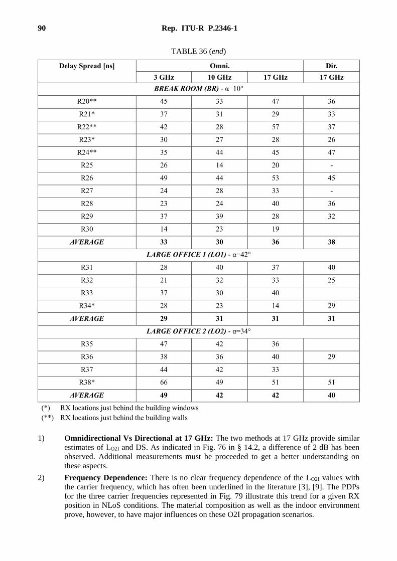
90 Rep. ITU-R P.2346-1
TABLE 36 (end)
Delay Spread [ns] Omni. Dir.
3 GHz 10 GHz 17 GHz 17 GHz
BREAK ROOM (BR) - α=10°
R20** 45 33 47 36
R21* 37 31 29 33
R22** 42 28 57 37
R23* 30 27 28 26
R24** 35 44 45 47
R25 26 14 20 -
R26 49 44 53 45
R27 24 28 33 -
R28 23 24 40 36
R29 37 39 28 32
R30 14 23 19
AVERAGE 33 30 36 38
LARGE OFFICE 1 (LO1) - α=42°
R31 28 40 37 40
R32 21 32 33 25
R33 37 30 40
R34* 28 23 14 29
AVERAGE 29 31 31 31
LARGE OFFICE 2 (LO2) - α=34°
R35 47 42 36
R36 38 36 40 29
R37 44 42 33
R38* 66 49 51 51
AVERAGE 49 42 42 40
(*) RX locations just behind the building windows
(**) RX locations just behind the building walls
1) Omnidirectional Vs Directional at 17 GHz: The two methods at 17 GHz provide similar
estimates of LO2I and DS. As indicated in Fig. 76 in § 14.2, a difference of 2 dB has been
observed. Additional measurements must be proceeded to get a better understanding on
these aspects.
2) Frequency Dependence: There is no clear frequency dependence of the LO2I values with
the carrier frequency, which has often been underlined in the literature [3], [9]. The PDPs
for the three carrier frequencies represented in Fig. 79 illustrate this trend for a given RX
position in NLoS conditions. The material composition as well as the indoor environment
prove, however, to have major influences on these O2I propagation scenarios.

Rep. ITU-R P.2346-1 91
FIGURE 79
PDPs across the frequency bands for R33
The DS values, lower than 50 ns for the most part (30 ns being approximately the delay spread in
LoS conditions) do not seem to display any dependence regarding the carrier frequency as well.
This observation is illustrated in Fig. 80 where the PDPs present overall the same shape.
FIGURE 80
Relative PDPs across the frequency bands for R33
14.4 Conclusion
In this paper, the propagation channel properties at 3, 10 and 17 GHz were studied for mmW
communication systems. For an O2I scenario, the building penetration losses and the channel delay
spread were determined.
The results revealed a strong variation in signal attenuation (from 10–40 dB) depending on the
room type and most definitely on the structure of the building exterior walls and/or windows.
Differences within the window glass compositions may explain such variations. Regarding the
frequency, the dependence is almost inexistent and is overshadowed by the variations caused by the
materials. The delay spread values are pretty low and also uniformly distributed (below 50 ns in
general for all the measurements) across the frequency bands.
At 17 GHz, the omnidirectional-equivalent characteristics (such as PDPs) obtained from directional
channel measurements were found similar to the characteristics extracted directly from
omnidirectional measurements. The utilized synthesizing procedure could be adopted at higher
frequencies where the use of directional antennas is required to compensate for the increased
propagation losses.
Measurements at higher frequency bands (60 GHz e.g.) are planned to extend the analysis of the
frequency-dependence for the O2I penetration losses and the channel delay spread.
3.8 3.9 4 4.1 4.2 4.3 4.4 4.5 4.6-50
-40
-30
-20
-10
0
Relative Delay Time (us)
No
rma
lize
d M
ag
nitu
de
(d
B)
3 GHz
10 GHz
17 GHz Omnidirectional
3.8 3.9 4 4.1 4.2 4.3 4.4 4.5 4.6-50
-40
-30
-20
-10
0
Relative Delay Time (us)
No
rma
lize
d (
Re
lative
) M
ag
nitu
de
(d
B)
3 GHz
10 GHz
17 GHz Omnidirectional
Threshold

92 Rep. ITU-R P.2346-1
14.5 References
[1] T. S. Rappaport, G. R. MacCartney, Jr., M. K. Samimi, and S. Sun, “Wideband Millimeter-Wave
Propagation Measurements and channel Models for future Wireless communication System
Design,” IEEE Transactions on Communications, vol. 63, no. 9, pp. 3029-3056, Sept. 2015.
[2] R. J. Weiler, M. Peter, W. Keusgen, and M. Wisotzki, “Measuring the Busy Urban 60 GHz Outdoor
Access Radio Channel,” IEEE International Conference on Ultra-Wideband (ICUWB), 2014.
[3] I. Rodriguez, H. C. Nguyen, N. T. K. Jorgensen, T. B. Sorensen and P. Mogensen, “Radio
Propagation into Modern Buildings: Attenuation Measurements in the Range from 800 MHz to
18 GHz,” IEEE, 2014.
[4] C. Larson, F. Harrysson, B.-E. Olsson and J.-E. Berg, “An Outdoor-to-Indoor Propagation Scenario
at 28 GHz,” IEEE European conference on antennas and Propagation (EuCAP), 2014.
[5] P. Okvist, H. Asplund, A. Simonsson, B. Halvarsson, J. Medbo and N. Seifi, “15 GHz Propagation
Properties Assessed with 5G Radio access Prototype,” IEEE on Personal , Indoor and Mobile Radio
Communications (PIMRC), 2015.
[6] J.-M. Conrat, P. Pajusco, and J. Y. Thiriet, "A Multibands Wideband Propagation Channel Sounder
from 2 to 60 GHz," in Instrumentation and Measurement Technology Conference (IMTC), Sorrento,
2006.
[7] S. Sun, G. R. MacCartney, M. K. Samimi, and T. S. Rappaport, “Synthesizing Omnidirectional
Antenna Patterns, Received Power and Path Loss from directional Antennas for 5G Millimeter-
Wave Communications,” in 2015 IEEE Global Communications Conference (GLOBECOM), Dec.
2015, pp. 3948-3953.
[8] A. Mitra, “Lecture Notes on Mobile Communications - Chapter 4: Free Space Radio Wave
Propagation,” Nov. 2009.
[9] H. Okamoto, K. Kitai and S. Ichitsubo, “outdoor-to-Indoor Propagation Loss Prediction in 800-
MHz to 8-GHz Band for an Urban Area,” IEEE Transactions on Vehicular Technology, vol. 58, no.
3, March. 2019.
15 Measurements in Stockholm in the 2-60 GHz frequency range
15.1 Introduction
In order to provide credible building entry loss modelling over the 5G frequency range,
experimental data in the mmWave range is required. Until recently, the amount of measurement
data available has been little. For this reason, an outdoor-to-indoor multi-frequency measurement
campaign was conducted in an eight stories tall office building in Kista covering the frequency
range 2 GHz to 60 GHz. Furthermore, Ericsson proposes a building entry loss model which is
validated and calibrated based on the herein presented measurement data.
The research leading to these results received funding from the European Commission H2020
programme under grant agreement No 671650 (mmMAGIC project).
15.2 Measurement campaign
A building entry loss measurement campaign was performed in an ‘old type’ of office building in
the Kista area of Stockholm, as depicted in Fig. 81. The transmitter was located in an open window
at the upper floor of the building and the received signal was measured at 2 slightly shifted (30 cm)
positions at 40 indoor locations across the inner yard on the same floor. Four different carrier
frequencies between 2.44 GHz and 58.68 GHz were measured at three different measurement
occasions over a few days. The basic details of the measurement set-up are given in Table 37. At
the upper floor of the building, the exterior wall is covered with metal. The windows are, however,

Rep. ITU-R P.2346-1 93
pure glass without metallization. It should be noted that there are three layers of glass in the window
frames resulting in some frequencies being substantially more attenuated than others with an
oscillating trend over the measured frequency range.
TABLE 37
Basic data of measurement setup
Carrier
frequency 2.44 GHz 5.8 GHz 14.8 GHz 58.68 GHz
Bandwidth 80 MHz 150 MHz 200 MHz 2 GHz
Transmit power 10 dBm 10 dBm 10 dBm 10 dBm
Antenna Tx (vert.
polar.) Patch ~7dBi Patch ~7dBi Open wave guide Open wave guide
Antenna Rx (vert.
polar.) Omni 2dBi Omni 2dBi Omni 2dBi Omni 2dBi
Tx Antenna height 1.5 m (ref : indoor floor)
Rx Antenna height 1.5 m (ref : indoor floor)
In order to avoid any bias due to the different bandwidths of the different frequencies, the measured
impulse responses are filtered down to 80 MHz for all frequencies. For some locations and
frequencies, 30 dB dynamic range was not possible to achieve. For these locations, the dynamic
range of the carrier frequency having the smallest dynamic range is used for all carrier frequencies
in order to avoid any frequency-dependent-bias.
FIGURE 81
Outdoor to indoor measurement scenario (left). The indoor Rx locations are marked with red-filled circles and the Tx
location is marked with a blue-filled circle. On the right hand side, a photograph of the building is shown
66 m
Tx

94 Rep. ITU-R P.2346-1
It can be observed from simulation and measurement, that for glass material, the penetration loss
will increase slowly with the increase of frequency. But for concrete material, the penetration loss
will increase sharply with the increase of the frequency.
Between 2.44 GHz and 14.8 GHz the building penetration loss ranges from around 0 dB up to
30 dB (Fig. 82). The lower end of penetration loss around 0 dB is similar for all frequencies while
the highest losses around 45 dB occur only at 58.68 GHz. Between 2.44 GHz and 14.8 GHz the
high end of penetration loss is between 25 dB and 30 dB. The proposed model (below) is based on
the exterior wall loss, due to penetration of the exterior wall only, combined with additional loss
due to further penetration into the building. Measurement locations of the Rx which are less than
4 m from the exterior wall facing the Tx experience exterior wall loss only, as there are no
obstructing objects between the Rx and the exterior wall. It is clear from Fig. 82 that the
corresponding exterior wall loss is in the range 0–20 dB over all frequencies.
FIGURE 82
Loss in excess of free space loss for the different frequencies in the outdoor to indoor measurements. On the left hand side,
the CDFs are shown and on the right hand side the loss as function of distance from the exterior wall which is in LOS with
respect to the transmitter is shown
The spread is substantially larger for the higher frequencies. In particular, the exterior wall loss at
58.68 GHz is over 20 dB at the 90 percentile level i.e. 10% of the locations experience more than
20 dB exterior wall loss. For 2.44 GHz and 14.8 GHz the 90 percentile level is only about 10 dB.
This difference may be explained by two effects. The first effect is interference due to multiple
layers of glass in the windows. The corresponding loss is particularly severe at 5.8 GHz (see
§ 15.3). The other effect is blocking by venetian blinds and window frames. As the blinds are at the
order of a couple of wavelengths at 58.68 GHz this effect becomes substantial at this frequency. At
locations where high building entry loss is experienced at 58.68 GHz it is likely that either the
blinds were down or that the window frame blocked line of sight. The window frame blocking
might explain why the loss actually goes down only at 58.68 GHz when the distance to exterior wall
increases.

Rep. ITU-R P.2346-1 95
FIGURE 83
Building penetration loss versus distance from exterior wall for the different frequencies at 10,
50 and 90 percentile levels
15.3 Monte Carlo simulation of multi-pane glass window transmission loss
To investigate the behaviour of how the multi-layered window glass impacts the frequency
dependency, a simulation has been made for a two-glass window with varied airspace in a realistic
interval. The result shows a strong frequency dependency and that the transmission loss (high or
low) seems quite stable for specific frequency bands. How and if this should be reflected in the BEL
model is still under consideration and may need more attention.
Simulation assumptions:
Two-pane layered standard glass with no metallization.
Airspace = 12-16 mm (uniformly distributed).
Glass thickness = 4 mm.
Relative permittivity of glass = 7.
Absorption loss of glass (tan 0.02.
Random polarization.
Penetr
atio
n lo
ss [dB
]
Distance from exterior wall [m] Distance from exterior wall [m] Distance from exterior wall [m]
10 percentile 50 percentile 90 percentile

96 Rep. ITU-R P.2346-1
FIGURE 84
Median +/- standard deviation (error bars) for a two-layer window simulation
16 Measurements at 5-31 GHz in China
16.1 Measurement scenarios
Two office buildings in China are measured, named as Building A, Building B, which have
different structure and material. Building A is with reinforced concrete shear wall and one-way
transparent glass which is with a thin metal coating. The thickness of the bearing wall is 35 cm ~
38 cm. In addition, the building's exterior wall is being equipped with thermal insulation material
whose structure is the foam polyethylene sheet and metal reflective layer. Building B is a modern
building combined the toughened glass with the reinforced concrete. The toughened glass is laid in
the wall which is known as a common toughened glass without metal coat.
16.1.1 Building A
Building A is with reinforced concrete shear wall structure, whose have exterior load-bearing walls
and some interior load-bearing walls. The thickness of the bearing walls is 35 cm ~ 38 cm. The
glass of windows of the building is known as one-way transparent glass which has a good visibility
from the inside to outside but a poor visibility from the outside to inside. This one-way transparent
glass is with a thin metal coating, so it will reflect the electromagnetic wave and bring big
penetration loss. In addition, the building's exterior wall is being equipped with thermal insulation
material whose structure is the foam polyethylene sheet and metal reflective layer.
The receiving antenna is on an outdoor platform which is on 4th floor. The pictures are shown in
Fig. 85. Only two operators are on the platform during the test, and they stay away from the
receiving antenna. The height of the transmitting antenna is 2.3 m, and the height of the receiving
antenna is 1.5 m.
The receiving point located on the 4th floor platform outdoor, the main receiving point is labelled as
R1, marked as blue point in Fig. 86. Some transmitting points on the 4th floor indoor are marked as

Rep. ITU-R P.2346-1 97
red point in Fig. 86. Other transmitting points on the 5th floor indoor are marked as red point shown
in Fig. 87. Furthermore the receiving points and transmitting points are marked with coordinate
values. R1 is the coordinate origin.
FIGURE 85
The receiving antenna located on the platform of Building A, 4th floor
Figure 85: The outdoor platform of the Building A: The building scene from the receiving point, the
thermal insulation layer is adding to the exterior wall of the Building A (Panoramic camera model.
Middle image of the building is slightly bent). There are no any other obstacles, e.g. trees between
the transmitter and receiver except the building.

98 Rep. ITU-R P.2346-1
FIGURE 86
The transmitting points indoor and the receiving points outdoor on the 4th floor,
the length of the platform is 28 m
FIGURE 87
The transmitting points indoor on the 5th floor
The coordinates of the receiving points and transmitting points in Building A are shown in
Table 38.

Rep. ITU-R P.2346-1 99
TABLE 38
The coordinates of the receiving points and transmitting points in Building A (unit: m)
Points x y z
R1 0 0 0
T1 0 29.6 4.7
T2 2.8 29.6 4.7
T3 2.8 33.4 4.7
T4 0.9 33.4 4.7
T5 5.1 34.2 4.7
T6 -6.8 35.3 4.7
T7 -10.6 35.5 4.7
T8 -18.1 35.4 4.7
T9 -14.9 32.6 4.7
T10 -11.7 31.4 4.7
T11 -15.4 38.3 4.7
T12 -37.9 36.9 4.7
T13 0 30.2 1.8
T14 2.8 30.5 1.8
T15 5.3 34.3 1.8
T16 5.9 35.5 1.8
T17 20.2 35.6 1.8
T18 19.1 40.6 1.8
T19 30.4 33.2 1.8
T20 33.7 17.8 1.8
T21 33.2 22.8 1.8
Some transmitting points’ pictures in Building A are shown in Figs 88 to 90.

100 Rep. ITU-R P.2346-1
FIGURE 88
The transmitting point in the corridor of the Building A

Rep. ITU-R P.2346-1 101
FIGURE 89
The transmitting point by the glass door of the Building A

102 Rep. ITU-R P.2346-1
FIGURE 90
The transmitting point in the stair channel of the Building A
16.1.2 Building B
Building B is a modern building combined the toughened glass with the reinforced concrete. The
toughened glass is laid in the wall which is known as a common toughened glass without metal
coat. Part of exterior wall is equipped with a brown ceramic tile. There is a parking lot outside the
building, the length of which is about 35 m. In order to avoid the influence of vehicle movement,
the method is:
– The test is taken at the weekend to make sure there are few vehicles and staffs.
– Make sure the receiving antenna away from the vehicle.
– The height of the receiving antenna is set to 2.3 m to ensure that the connection between the
transmitting antenna and the receiving antenna is not blocked by vehicles.
The main receiving point is R3, which is marked with blue point in Fig. 92, and the transmitting
points on the 1st floor are marked with red point in Fig. 92. The transmitting points on the 2nd floor
are marked with red points in Fig. 93. The transmitting points on the 3rd floor are marked with red
point in Fig. 94. The height of the transmitting antenna is 2.3 m and the height of the receiving
antenna is 2.3 m from the floors at that time.

Rep. ITU-R P.2346-1 103
FIGURE 91
Receiving antenna in the parking lot of Building B
Figure 91 Parking lot outside the Building B: The building scene from the receiving point. There
are no any other obstacles, e.g. trees between the transmitter and receiver except the building.

104 Rep. ITU-R P.2346-1
FIGURE 92
The transmitting points indoor and the receiving point outdoor on the 1st floor in Building B,
the length of the outdoor parking lot is 35 m

Rep. ITU-R P.2346-1 105
FIGURE 93
The transmitting points on the 2nd floor in Building B

106 Rep. ITU-R P.2346-1
FIGURE 94
The transmitting points on the 3rd floor in Building B
A coordinate system is formed with the R3 being a coordinate origin. The coordinates of the
transmitting points and receiving point are shown in Table 39.
TABLE 39
The coordinates of the receiving points and transmitting points in Building B (unit: m)
Points x y z
R3 0.0 0.0 0.0
T23 0.0 -45.5 0.0
T24 -13.5 -45.5 0.0
T25 -13.5 -37.5 0.0
T26 -14.4 -60.8 0.0
T27 -11.6 -62.7 0.0
T28 7.8 -45.5 0.0
T29 14.8 -49.7 0.0
T30 23.9 -38.7 0.0
T31 13.8 -38.7 0.0
T32 22.1 -31.3 4.6
T33 13.0 -34.7 4.6
T34 11.9 -34.5 4.6
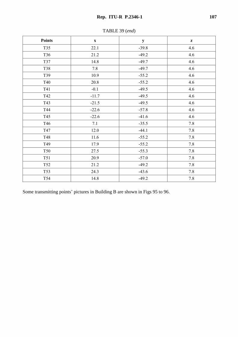
Rep. ITU-R P.2346-1 107
TABLE 39 (end)
Points x y z
T35 22.1 -39.8 4.6
T36 21.2 -49.2 4.6
T37 14.8 -49.7 4.6
T38 7.8 -49.7 4.6
T39 10.9 -55.2 4.6
T40 20.8 -55.2 4.6
T41 -0.1 -49.5 4.6
T42 -11.7 -49.5 4.6
T43 -21.5 -49.5 4.6
T44 -22.6 -57.8 4.6
T45 -22.6 -41.6 4.6
T46 7.1 -35.5 7.8
T47 12.0 -44.1 7.8
T48 11.6 -55.2 7.8
T49 17.9 -55.2 7.8
T50 27.5 -55.3 7.8
T51 20.9 -57.0 7.8
T52 21.2 -49.2 7.8
T53 24.3 -43.6 7.8
T54 14.8 -49.2 7.8
Some transmitting points’ pictures in Building B are shown in Figs 95 to 96.

108 Rep. ITU-R P.2346-1
FIGURE 95
The transmitting point in the lobby on the 1st floor in Building B
(In transmitting point the receiving point can be seen through glass)

Rep. ITU-R P.2346-1 109
FIGURE 96
The transmitting point next to the elevator on the 2nd floor in Building B
16.2 Test methodology
In Building A and B, 11 frequency points are selected for each frequency band, e.g. 3.5 GHz,
5 GHz, 15 GHz, 24 GHz, 28 GHz and 31 GHz.
16.2.1 Measuring system and instrument
The devices of measuring system are shown in Table 40.

110 Rep. ITU-R P.2346-1
TABLE 40
The antenna selection consideration
Transmitting antenna Omni-directional vertical polarization antenna (for 3.5 GHz)
Horn vertical polarization antenna for 5-31 GHz band
Receiving antenna Omni-directional vertical polarization antenna. (for 3.5 GHz)
Horn vertical polarization antenna for 5-31 GHz band
Transmitter Agilent E8267D signal generator
RF power amplifier The output power in the test is set to 33 dBm for 3.5 and 20 dBm for 5-
31 GHz band
Receiver Agilent N9030A signal analyser
We have developed an automatic program in order to control instruments and record test data by
LAN. In each location and frequency points, 500 continuous reading is got which will cost about
8 ~ 10 seconds.
16.3 Calculation method of building entry loss
The free space loss can be calculated as:
32.45 20lg 20lgf m GHzL d f (17)
Where d is defined in Fig. 97. f is carrier frequency in GHz. Set transmitted power be Pt (dBm) and
received power be Pr (dBm), the building entry loss is expressed as LE, transmitting antenna gain
and receiving antenna gain in transmission path are expressed as Gt and GR, relatively.
FIGURE 97
The location relationship between the receiving antenna and the transmitting antenna
TxAntenna
RxAntennad
EL RG
TG
rP
tP
Then we can get equation (18).
t f E rt dBm r dBmP G L L G P (18)
And then equation (19) can be deduced from equation (18).

Rep. ITU-R P.2346-1 111
E f t rt dBm r dBmL P P L G G (19)
For Omni-directional antenna used in the 3.5 GHz test, the antenna pattern is similar to half wave
dipole antenna whose gain is 2.15 dB, and the normalized directivity function of electric field of
half-wave dipole antenna is expressed as equation (20).
sinF (20)
Where θ is defined in Fig. 97. From equation (20), we can get equation (21).
4 44.3 10lg 4.3 10lg sint rG G F (21)
For horn antenna case, the receiving antenna gain is properly considered in calculation.
16.4 Measurement results
The median values of building entry loss measured above are shown in Table 41. The categories of
all links from transmitters and receivers can be separated as three types:
The ‘depth/penetration’ categories are as follows:
C1 Indoor terminal in a room/space with an external wall facing the outdoor terminal
C2 Indoor terminal in a room/space with no external walls (e.g. stairwell, corridor)
C3 Indoor terminal in a room/space with an external wall not facing the outdoor terminal
TABLE 41
The median value of entry loss (Building A, Unit: dB)
Frequency
(GHz)
3.5 5 15 24 28 31
Tx 1 31.71 39.48 34.62 25.24 41.60 37.13
Tx 2 20.98 26.58 47.64 52.40 58.95 59.32
Tx 3 24.19 24.73 36.62 26.38 42.39 39.75
Tx 4 26.17 33.61 41.32 20.88 46.78 41.96
Tx 5 43.42 50.08 54.95 48.49 69.15 58.14
Tx 6 43.98 52.40 72.23 69.60 75.33 73.98
Tx 7 45.74 55.09 71.84 74.96 73.03 70.91
Tx 8 47.11 54.52 59.66 65.61 65.67 64.31
Tx 9 29.69 31.90 45.00 43.92 53.55 57.68
Tx 10 27.23 36.83 38.19 38.28 49.65 51.44
Tx 11 58.84 61.20 65.08 70.28 68.39 66.84
Tx 12 55.97 21.92 13.01 57.45 49.40 47.36
Tx 13 35.15 36.99 37.20 28.10 34.32 37.38
Tx 14 33.71 27.57 36.34 42.14 54.65 59.05
Tx 15 52.22 48.11 57.93 54.80 57.00 64.71
Tx 16 54.55 60.79 69.57 57.49 65.33 62.61
Tx 17 49.92 41.14 52.48 62.43 63.89 62.00
Tx 18 68.64 57.09 60.54 65.79 65.88 64.82

112 Rep. ITU-R P.2346-1
Frequency
(GHz)
3.5 5 15 24 28 31
Tx 19 63.65 34.25 22.26 81.56 81.02 79.45
Tx 20 36.38 21.28 12.77 53.86 54.86 62.33
Tx 21 50.48 18.32 10.90 51.50 58.28 64.28
16.4.1 Measurement results and analysis of Building B scenario
After processing the original test data the entry loss of Building B can be got. The median value of
the entry loss measurement above is shown in Table 42. The categories of all links from
transmitters to receivers are the same with Building A. It should be noted that 5 GHz and 15 GHz
case is not been tested in this building.
TABLE 42
The median value of the Entry loss (Building B, Unit: dB)
Frequency
(MHz)
3.5 24 28 31
Tx 23 11.16 15.39 13.27 13.86
Tx 24 16.64 22.77 21.19 20.22
Tx 25 15.78 19.39 22.80 22.39
Tx 26 13.01 25.66 27.96 23.92
Tx 27 19.23 40.02 37.99 39.28
Tx 28 15.54 16.64 28.19 28.50
Tx 29 25.96 32.94 33.56 37.14
Tx 30 21.97 35.31 38.82 38.24
Tx 31 19.37 27.52 34.49 35.57
Tx 32 38.44 47.51 52.72 52.21
Tx 33 32.37 49.57 49.76 49.40
Tx 34 27.85 43.51 45.59 45.74
Tx 35 26.02 43.97 43.63 49.92
Tx 36 38.15 44.04 46.34 49.41
Tx 37 38.55 65.28 66.76 64.40
Tx 38 22.02 26.78 34.14 22.88
Tx 39 35.52 50.71 60.16 61.95
Tx 40 41.33 49.01 53.45 58.04
Tx 41 20.25 18.00 22.00 27.15
Tx 42 21.63 24.79 32.64 31.94
Tx 43 35.14 42.81 51.34 47.96
Tx 44 43.55 56.37 61.69 60.83
Tx 45 34.55 41.43 42.92 45.21
Tx 46 22.00 28.74 27.41 28.53
Tx 47 32.84 28.74 35.59 41.65
Tx 48 49.50 74.86 73.91 72.20

Rep. ITU-R P.2346-1 113
Frequency
(MHz)
3.5 24 28 31
Tx 49 56.38 25.98 30.90 37.13
Tx 50 56.66 61.68 61.63 60.21
Tx 51 64.87 -- -- --
Tx 52 56.09 57.05 59.31 57.69
Tx 53 44.73 49.92 52.58 54.96
Tx 54 53.67 72.10 70.34 68.34
17 Measurements below 6 GHz in a modern office building
17.1 Method
The method adopted was the same as that used in the previous study and follows the
recommendations given in § 4 of Recommendation ITU-R P.2040-1.
17.2 Locations
A major constraint in conducting measurements of building loss in urban areas is that it is very
difficult to ensure that the measurement path has a clear line-of-sight to the building under
investigation. If this condition is not met, the measured data will necessarily include an unknown
element of local clutter loss.
The waterfront location of Ofcom (“Riverside House”) offered an opportunity to avoid this
problem, and a building with a roof terrace was identified on the opposite side of the river, offering
a clear line-of-sight to the front of the target offices.
FIGURE 98
Riverside House seen from receiver location

114 Rep. ITU-R P.2346-1
As for the earlier tests, the receiver was at the fixed outdoor location (simply because of the bulk of
the spectrum analyser used), while the portable indoor terminal consisted of a set of compact CW
transmitters developed for the earlier work.
FIGURE 99
View towards receiver site (arrowed) from Floor 11 of Riverside House
FIGURE 100
View towards receiver site (arrowed) from Floor 3 of Riverside House
The receiver terminal was set up on the south-west corner of the terrace, with antennas supported on
a 1.6 m tripod. The height above the river (wrt chart datum) was 24 metres.

Rep. ITU-R P.2346-1 115
The 230 metre path between the receiver and the front of riverside House is shown in Fig. 101.
FIGURE 101
Showing 230 metre path from Riverside House (south) to 10 Queen Street Place (north)
A sketch of the locations in elevation is shown in Fig. 102. This Figure also indicates the direct and
river-reflected paths to a measurement location on the third floor of Riverside House (see discussion
below). The height of the measurement antennas above river level (chart datum) was 23 m (floor 2),
26 m (floor 3) and 52 m (floor 11).
FIGURE 102
Sketch of locations (not to scale)

116 Rep. ITU-R P.2346-1
17.3 Measurement procedure
Measurements were made at five frequencies9 , using the same equipment developed for the earlier
measurements. The frequencies used were 8710 MHz, 217 MHz, 69011 MHz, 2 410 MHz and
5 760 MHz.
Following the Recommendation ITU-R P.2040 method, the measurement approach was statistical,
in that no attempt was made to record the instantaneous position of the portable indoor terminal,
Instead, the statistical distribution of received power was recorded in a series of small areas
(‘zones’) within Riverside House. This will allow the parameterisation of building loss statistics in
terms of depth within the building. The median received power in each zone is compared with a
reference measurement made on the balcony of the relevant floor to derive the BEL.
Measurements were carried out on Floors 2, 3 and 11 of Riverside House. The two lower floors
were each divided into eight measurement zones, while three zones were used on the upper floor.
Plans showing the location of the zones are given in Annex C.
Measurements were made separately for each frequency, to avoid issues with antenna combining
and interaction. The transmitter was carried around each zone in turn, with the receiver12 logging
received power at a sampling interval of 78 ms. No attempt was made to follow precisely the same
path at different frequencies; earlier work has shown that median measured values are repeatable to
within <1 dB using this method.
FIGURE 103
Indoor measurements (5.7 GHz)
9 Measurements were also made at 3 550 MHz, using equipment funded under a separate study. The results
of these measurements have been submitted to CG 3J-3K-3M
10 Changed from previous frequency (88.8 MHz) due to local FM radio services
11 Changed from previous frequency (698 MHz) due to local digital TV services
12 A Rohde & Schwarz FSP13 spectrum analyser

Rep. ITU-R P.2346-1 117
At a typical walking pace of 1 m/s, the receiver was sampling 44 times in a wavelength at 87 MHz
and only 0.7 times at 5 760 MHz; reciprocally, only 23 wavelengths were explored at 87 MHz in a
typical measurement length of 80 metres, but 1 428 wavelengths were covered at 5 760 MHz. The
under-sampling at higher frequencies would be of concern if a record of median field along the path
were required, but is acceptable in the context of deriving loss statistics for the each ‘zone’ as a
whole.
FIGURE 104
Portion of data logged in Zone 5, floor 2 at low (left) and high (right) frequencies
These very different sampling regimes have implications for data processing, and in particular limit
the rigour with which multipath and shadow fading may be separated. In a more elaborate
experiment sampling at a constant spatial or wavelength interval might be arranged, but this was not
permitted by time and logistics. An alternative approach would be to employ a wideband channel
sounder, but the bandwidth available would be very limited at the lower frequencies.
The path length to Riverside House is 230 m and the depth of the building is 50 m. This would
correspond to an additional free space path loss of 1.7 dB. A small correction was made to each of
the measured median entry loss values to account for this additional spreading loss13.
17.4 Reference measurements
In line with the ITU-R Recommendation, and the measurements made in the earlier Ofcom study,
the building entry loss is defined relative to the median field measured immediately outside the
building, on the balcony of each floor.
These measurements were made by walking back and forth while holding the transmit antenna clear
of local obstructions, and in clear sight of the receive location. These ‘reference’ measurements
were made both before and after each set of indoor measurements as a check that no faults had
developed with the transmit or receive systems.
13 0.2 dB in zones 1 & 2, 0.4dB in zone 3, 0.5 dB in zones 4-6, 0.8 dB in stairwell, 0.9 dB in zone 7 and
1.4 dB in zone 8.

118 Rep. ITU-R P.2346-1
FIGURE 105
Reference measurement on 11th floor balcony, showing receiver terminal location
It can be seen that there are a number of metallic obstructions on and around the balcony, and the
received signal shows significant multipath effects as a result. As the intention is to confirm the
strength of the field incident on the face of the building, rather than to observe local effects, the
time-series record of received power was examined to identify portions where the received signal
showed no sign of shadow fading, and a median was taken through the multipath (see Fig. 106).
The value so derived should correspond to the free-space field (except, perhaps, at the lowest
frequencies where coherent ground/water reflections might distort the results).
FIGURE 106
Balcony reference measurement (floor 3)
Link budgets are given in an annex, and a comparison between the predicted free-space power at
the receiver and that actually measured is given in the Table below.

Rep. ITU-R P.2346-1 119
TABLE 43
Predicted and measured ‘outdoor reference’ powers
Frequency 87 MHz 217 MHz 690 MHz 2410 MHz 5760 MHz
RX power (free-space) −29.1 −41.2 −52.0 −50.4 −55.7
Measured floor 11 −32.1 −45.0 −51.1 −54.5 −57.0
Measured floor 3 −34.1 −41.2 −51.3 −51.4 −56.5
Measured floor 2 −34.8 −41.1 −51.2 −51.4 −56.3
In all cases except at 87 MHz, the measured and predicted fields on the lower floors agree to within
1 dB. The significant discrepancy (5.0-5.7 dB) at the lowest frequency may be due to coupling
between the transmit aerial and the large amount of metalwork on the balcony at distances less than
a wavelength.
Another possibility is that of destructive interference between the direct and river-reflected rays
sketched in Fig. 101. The impact of this is difficult to predict as the heights of the buildings relative
to the river vary with the tide, and the reflection point may fall in the river or on the bridge (see
Fig. 100). It is, nevertheless, instructive to plot the predicted path loss variation with terminal height
at Riverside House (see Fig. 107), which suggests that for certain transmit terminal heights the field
at the receiver may be more than 2 dB below free-space.
FIGURE 107
Loss as a function of transmitter height (87 MHz)
While the signals measured on the lower two balconies show a very close correspondence (with a
maximum discrepancy of 0.7 dB between measurements made on floor 2 and floor 3), the same is
not true for the 11th floor. In this case, only the 690 and 5 760 MHz results are close to those, and a
2-4 dB discrepancy at other frequencies. No explanation has been found for this – it cannot be

120 Rep. ITU-R P.2346-1
attributed to the modest increase in elevation angle, as the vertical beamwidth of none of the
antennas used would account for more than a fraction of one dB of additional attenuation.
Given the generally good agreement between prediction and the ‘balcony reference’ values, the
latter will be used to determine the BEL values on each floor, as in the previous study and as
recommended in Recommendation ITU-R P.2040. The uncertainties in the reference values at
87 MHz, and on the 11th floor should be borne in mind when examining the results, however.
17.5 Results
17.5.1 Building entry loss (median loss)
The ‘headline’ figure of interest is the difference between the median field that would be received in
the absence of the building, and that actually measured.
The median signal level was determined for each of the measurements sets made in each zone, and
these are plotted below.
FIGURE 108
Median loss values (floor 2)

Rep. ITU-R P.2346-1 121
FIGURE 109
Median loss values (floor 3)
FIGURE 110
Median loss values (floor 11)
It can be seen that, as would be expected, the median loss increases as the mobile terminal moves
further inside the building. In zone 1, by the windows facing the transmitter, losses are typically
20 dB less than at the back of the building.
The trend with frequency is interesting, with the highest losses seen at 87 MHz, falling to a
minimum at 2.4 GHz and increasing again at the highest frequency. This trend is made more
explicit in Fig. 111.

122 Rep. ITU-R P.2346-1
FIGURE 111
Trend of BEL with frequency
A similar non-monotonicity, although with the minimum around 217 MHz, was seen in the earlier
measurements in domestic buildings, and can be explained qualitatively by observing that building
apertures are too small to permit efficient propagation at longer wavelengths, while higher
frequencies will tend to suffer more absorption by building materials.
17.5.2 Building entry loss statistics
While the median loss value may be a useful ‘headline’ figure, a radio system designer concerned
with ensuring the availability of a wanted signal, or protection from a potential interfere, will
generally be interested in other points on the statistical distribution.
The measurements made in all zones on each floor have been aggregated and the cumulative
distributions of the BEL derived (Fig. 112).

Rep. ITU-R P.2346-1 123
FIGURE 112
CDF of building entry loss (floors 2 and 3)
In the Figure, it can be seen that the results for the two floors are broadly similar, though with
differences in detail. The interdecile range is about 30 dB at lower frequencies, falling to 20 dB at
5.7 GHz.
It should be borne in mind that these statistics include multipath fading, so the range of losses seen
for wideband signals will be rather smaller; further processing should be undertaken to estimate the
variability associated with flat fading (absorption and diffraction) alone.
The losses measured in the present study are significantly (20-30 dB) greater than those seen in the
measurements made of domestic buildings, presumably due to a combination of the much greater
depth of the building and the large amount of metalwork in the construction. Even in zones 1 and 2,
immediately adjacent to the windows, losses are 10-20 dB greater than seen in either the terraced
house or the mansion at BRE.
It would be expected that the office windows would be metallised for thermal efficiency, and these
results would appear to confirm this; no data has yet been obtained on the characteristics of the
glass, however.
17.6 Conclusions
The attenuation suffered by radio waves entering Riverside House is substantially greater than was
the case for the domestic buildings measured previously.
Median entry loss was found to vary monotonically with depth within the building, but non-
monotonically with frequency, with the highest losses observed at VHF frequencies and at 5.7 GHz.
Evaluated over each floor of the building, 90% of losses were greater than 20 dB (690 MHz,
2.4 GHz) – 30 dB (87 MHz).
In making use of this measurement data it should be borne in mind that Riverside House may not be
representative of the generality of urban office buildings.
17.7 Annex - link budgets
The Table below gives the link budgets for the equipment and reference locations used in the trials.

124 Rep. ITU-R P.2346-1
TABLE 44
Link budgets
Frequency 87 MHz 217 MHz 690 MHz 2410 MHz 5760 MHz
TX power (dBm) 27.0 19.0 18.4 25.4 27.5
Feeder loss (dB) 0.4 0.8 1.4 1.4 2.2
TX ant gain (dBi) 1.7 2.0 1.6 3.0 1.5
e.i.r.p. (dBm) 28.3 20.2 18.6 27.0 26.8
Isotropic path loss (dB) 58.5 66.4 76.5 87.3 94.8
RX ant gain (dBi) 1.3 5.3 6.4 11.0 14.0
Feeder loss (dB) 0.2 0.3 0.5 1.1 1.7
Free space Rx power
(dBm)
−29.1 −41.2 −52.0 −50.4 −55.7
17.8 Annex - measurement zones at Riverside House
FIGURE 113
Floor 2 measurement zones
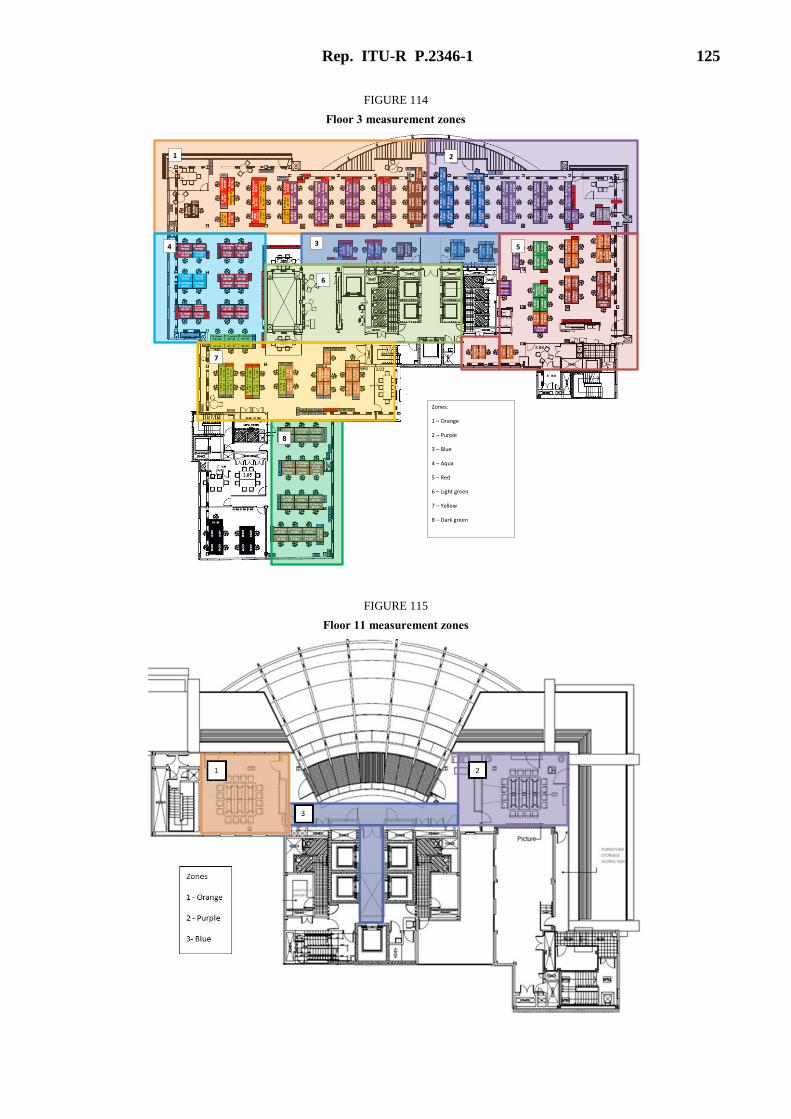
Rep. ITU-R P.2346-1 125
FIGURE 114
Floor 3 measurement zones
FIGURE 115
Floor 11 measurement zones
Zones:
1 – Orange
2 – Purple
3 – Blue
4 – Aqua
5 – Red
6 – Light green
7 – Yellow
8 – Dark green
4
1 2
3 5
6
6
7
8

126 Rep. ITU-R P.2346-1
18 Building loss in an urban environment (Japan, 0.8-37 GHz)
Measurements have been made of the building entry loss to an office building at six frequencies
between 0.8 and 37 GHz.
18.1 Measurement methods and parameters
This Section described the measurement method and parameters. Figures 116 to 118 respectively
show photographs of the measurement area taken at one of the Tx positions, at a corridor inside the
building and outdoor buildings. We regard as the glass window of the measurement route (marked
yellow point) as an LOS environment from a Tx position in the measurement environment. The tall
buildings surround the road in the measurement site. Figures 119 to 121 show the measurement
route and Table 45 summarizes the measurement parameters. To analyse the frequency
characteristics from microwave bands to millimeter wave bands, we set the measurement
frequencies at 0.8, 2.2, 4.7, 8.4, 26.3 and 37.0 GHz, respectively. The continuous waves (CW) were
simultaneously transmitted from the Tx antennas, which were set up on the roofs of cars positioned
on the roadside outside as shown in Fig. 116. Rx antenna was located in the indoor building. The Tx
antenna positions are shown as A1 and A2 in Fig. 119. We took repeated measurements on the 1st,
2nd, 4th, 6th and 8th floors (i.e. 1F, 2F, 4F, 6F and 8F). We also obtain the 3D incident angle
characteristics described in Fig. 6. Tx antennas were located at A-1 and A-2. Tx antenna height was
2.5 m above the ground. The Rx antenna was set up on a hand truck inside the building, and
measurements were carried out with the car running as shown in Figs 120 and 121. The Rx antenna
height was 1.5 m above the floor. The radiation patterns of the Tx and Rx antennas are omni-
directional in a horizontal plane. We note that vertically polarized waves were transmitted and
received in these measurements. The median value of path loss calculated every 1 metre.
FIGURE 116
Building from Tx position

Rep. ITU-R P.2346-1 127
FIGURE 117
Measurement route at indoor corridor
FIGURE 118
Outdoor building from 6F
FIGURE 119
Outdoor building layout and Tx positions
Tx positions
Building
of measurement
Building
Building
A1 A2

128 Rep. ITU-R P.2346-1
FIGURE 120
Top view of indoor environment and measurement route
FIGURE 121
Vertical view of indoor environment and measurement route
TABLE 45
Measurement parameters
Frequency (GHz) 0.8, 2.2, 4.7, 8.5, 26.4, 37.1
Tx antenna height 2.5 m
Rx antenna height 1.5 m
Floor number of measurement 1F, 2F, 4F, 6F and 8F
Tx/Rx antenna radiation pattern Omni-directional
18.2 Measurement results from 0.8 to 37.1 GHz band
In this section, we describe the measured path loss characteristics from the 0.8 to the 37.1 GHz
band. Figure 122 shows the path loss measurement results obtained at A-2 at 37.1 GHz for the route
for floors 1F, 2F, 4F, 6F and 8F. The horizontal axis indicates Rx moving distance along the
measurement route. The vertical axis indicates the normalized path loss. Figure 123 shows those
path loss slope of measurement results for each floor. Figure 124 shows the measurement results
obtained at A-2 on 8F for the 0.8, 2.2, 4.7, 8.5, 26.4 and 37.1 GHz frequency bands. Figure 125
shows the frequency dependence of measurement path loss. The horizontal axis indicates the
median value of path loss. The vertical axis indicates the frequency. In order to analyse the path loss
dependence on the frequency and 3D incident angle, the building entry loss BELmeas is normalized
27
.0 m
Mea
sure
men
t ro
ute
1.6 m 3.0 m
Yard
Glass window
18.4 m
Tx
Rx
Measurement
route
dout
din
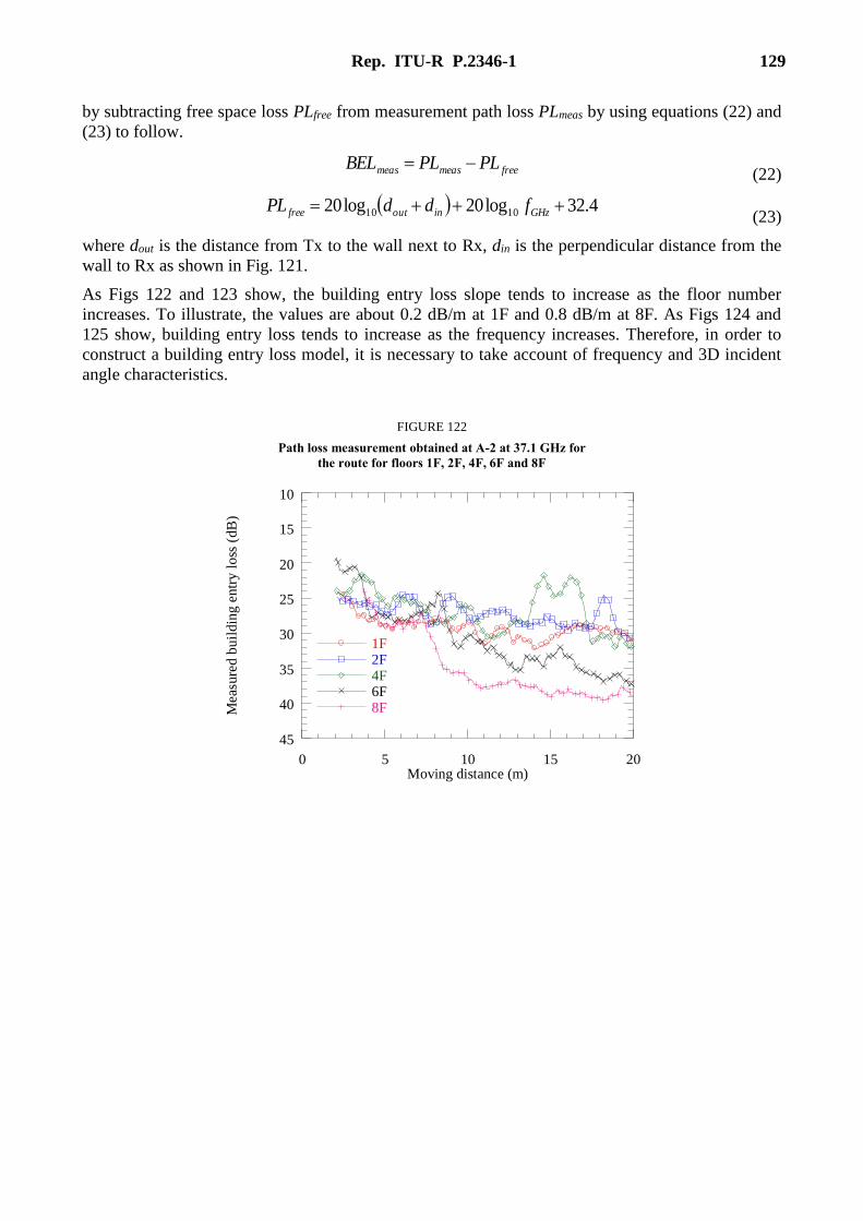
Rep. ITU-R P.2346-1 129
by subtracting free space loss PLfree from measurement path loss PLmeas by using equations (22) and
(23) to follow.
freemeasmeas PLPLBEL (22)
4.32log20log20 1010 GHzinoutfree fddPL
(23)
where dout is the distance from Tx to the wall next to Rx, din is the perpendicular distance from the
wall to Rx as shown in Fig. 121.
As Figs 122 and 123 show, the building entry loss slope tends to increase as the floor number
increases. To illustrate, the values are about 0.2 dB/m at 1F and 0.8 dB/m at 8F. As Figs 124 and
125 show, building entry loss tends to increase as the frequency increases. Therefore, in order to
construct a building entry loss model, it is necessary to take account of frequency and 3D incident
angle characteristics.
FIGURE 122
Path loss measurement obtained at A-2 at 37.1 GHz for
the route for floors 1F, 2F, 4F, 6F and 8F
10
15
20
25
30
35
40
45
0 5 10 15 20
1F2F4F6F8FM
eas
ure
d b
uil
din
g e
ntr
y l
oss
(d
B)
Moving distance (m)

130 Rep. ITU-R P.2346-1
FIGURE 123
Normalized path loss slope for floors 1F, 2F, 4F, 6F and 8F
FIGURE 124
Path loss measurement obtained at A-2 on 8F for the 0.8, 2.2,
4.7, 8.5, 26.4 and 37.1 GHz frequency bands
0.1
0.2
0.3
0.4
0.5
0.6
0.7
0.8
0.9
0 2 4 6 8 10
Buil
din
g e
ntr
y l
oss
slo
p (
dB
/m)
Floor number
10
15
20
25
30
35
40
45
0 5 10 15 20
0.8 GHz2.2 GHz8.5 GHz4.7 GHz26.4 GHz37.1 GHz
Mea
sure
d b
uil
din
g e
ntr
y l
oss
(d
B)
Moving distance (m)

Rep. ITU-R P.2346-1 131
FIGURE 125
Frequency dependence of median value of normalized path loss for the
0.8, 2.2, 4.7, 8.5, 26.4 and 37.1 GHz frequency bands
Annex 1
Building entry loss in point-to-area applications below 3 GHz
The following information has been found helpful in planning broadcast and other point-to-area
radio services.
For indoor reception two important parameters must also be taken into account. The first is the BEL
and the second is the variation of the BEL due to different building materials. The standard
deviations, given below, take into account the large spread of BEL but do not include the location
variability within different buildings. It should be noted that there is limited reliable information
and measurement results about BEL. Provisionally, BEL values that may be used are given in
Table A1.1.
TABLE A1.1
Building entry loss(1), Lbe, be
F Median value, Lbe
(dB)
Standard deviation, σbe
(dB)
0.2 GHz 9 3
0.6 GHz 11 6
1.5 GHz 11 6
(1) These values may have to be updated when more experimental data become available.
For frequencies below 0.2 GHz, Lbe = 9 dB, σbe = 3 dB; for frequencies above 1.5 GHz, Lbe = 11 dB,
σbe = 6 dB. Between 0.2 GHz and 0.6 GHz (and between 0.6 GHz and 1.5 GHz), appropriate values
24
26
28
30
32
34
36
38
0.1 1 10 100
Med
ian
valu
e o
f b
uil
din
g e
ntr
y l
oss
(dB
)
Frequency (GHz)

132 Rep. ITU-R P.2346-1
for Lbe and σbe can be obtained by linear interpolation between the values for Lbe and σbe given in
Table 7 for 0.2 GHz and 0.6 GHz (0.6 GHz and 1.5 GHz).
The field-strength variation for indoor reception is the combined result of the outdoor variation, L,
and the variation due to building attenuation, be. These variations are likely to be uncorrelated.
The standard deviation for indoor reception, i can therefore be calculated by taking the square root
of the sum of the squares of the individual standard deviations.
22beLi dB (24)
where σL is the standard deviation of location variability.
For example, for digital emissions with bandwidth greater than 1 MHz, at VHF, where the signal
standard deviations are 5.5 dB and 3 dB respectively, the combined value is 6.3 dB. In Band IV/V,
where the signal standard deviations are 5.5 dB and 6 dB, the combined value is 8.1 dB.
______________