complete solution of the three-compartment model in … · solution of three-compartment model in...

Complete solution of the three-compartment model in steady state after single injection of radioactive tracer1

S. M. SKINNER, R. E. CLARK, N. BAKER2 AND R. A. SHIPLEY Department of Chemistry and Chemical Engineering, Case Institute of Technology, the Radioisutu~e Service, Veterans Administration Hus/Gtal,

and Departments of Biochemistry and Medicine, Western Reserve Uni- versity School of Medicine, Cleveland, Ohio

SKINNER, S. M., R. E. CLARK, N. BAKER AND R. A. SwPu3Y. Complete solution of the thwe-compartment model in steady state after single injection of radioactive tracer. Am. J. Physiol. Ig6(2): 2@-244. Ig5g.-solutions of a general, three- compartment model in a nonisotopic steady state are developed. By means of these solutions, the investigator may analyze a great variety of kinetic flow relationships utilizing only algebraic procedures. Values of compartment sizes, rates of transport and specific activity-time curves are obtained for three typical hypothetical examples. Possible degrees of freedom and the use of parameters are examined. For those models where physical limitations prevent sufficient independent observations to allow completely determinate solutions, possible limiting values are established.

I N TRACER STUDIES of physiological and biochemical processes, the compartment or pool concept generally facilitates mathematical interpretation. The .potential complexity of many models and the attending mathematical treatment often invites simplification to the point that much meaningful information is obscured or lost entirely in the final analysis. Recently, however, Robertson (I) has presented an excellent comprehensive review of more complex solutions. The present analysis is intented to simplify the mathematical treatment of a general nonrestricted three-compartment model when a single injection of isotope is made into one compartment: It provides a straightforward method of analysis for a great variety of models, whether physiological, biochemical or physical. Values sought are those for individual pool sizes and rates of transport.

Received for publication. January 14, 1958. l This work was partially supported by the Office of Ordnance

Research, U. S. Army. Presented before the Radiation Research Society, Rochester Meeting, May I 4, 1957.

2 Present address : Radioisotope Service, Veterans Administra- tion Center, Los Angeles, Calif.

The pool system to be treated, as shown in figure I, includes all possible interconnections and routes of ingress and egress. By suppression of various channels of Aow so that the corresponding constants are zero the general model can be converted into one of many restricted forms such as are illustrated in figure 2. Setting all values of ingress and egress to zero gives a closed model. General solutions for the model under considera- tion have been developed in the brilliant matrix treatment of Berman and Schoenfeld (2). The actual analysis of experimental data by matrix methods, however, becomes complex, especially in cases where the number of measurable parameters is smaller than the number of variables. In such an instance the computational effort may be prohibitive. In the present analysis an alterna- tive direct method of obtaining the solution is carried through to the point at which only algebraic operations are necessary on the part of the experimenter.

FORMULATION OF FLOW EQUATIONS

The size of a compartment (labeled and unlabeled material) will be designated by Qi3 with its appropriate subscript, and the quantity of radioactive material instantaneously present in it by pi. Flow produces a dependence of pi on time, commencing with the known initial conditions, and ending in the final equilibrium.

No delay time or lag in mixing is assumed; the effects of such a delay may be treated by the introduction of additional compartments or by a more complex analysis. Let kdj be the value of the flow of total (labeled + unlabeled) material into compartment i from compartment j, i.e. the quantity per unit time passing into i from j. I f compartment j is of size Qi and contains ~j labeled material, the fraction of k;j which is labeled material is qj/Qj (specific activity), and the rate of de-

3 The subscript i or j is a nonspecific symbol which in final application of the formula becomes I, z or 3 according to the corresponding pool number.

23b

by 10.220.33.4 on June 18, 2017http://ajplegacy.physiology.org/

Dow

nloaded from

http://ajplegacy.physiology.org/

SOLUTION OF THREE-COMPARTMENT MODEL IN STEADY STATE 239

crease of labeled material in compartment j by flow into i is -(Q/Q&+ Th is, with sign changed, is also the rate of increase of labeled material in compartment i by flow from j. The rate constant Xij is defined by kij/Qj. Flow into the system, li, represents diluting material of zero activity (see fig. I). The flow equations are :

pool 1: - = dt

--x11 41 + x12 42 + x13 43

d42 Pool 2: - = x21 41 - x22 42 + x23 q3 dt 0 I

d43 pool 3: - = dt

x31 ql + x32 42 - x33 43 Y

where

x11 = x01 + x21 + x31

x22 = x02 + h2 + x32

x 33 = x03 + x13 + x23=

BOUNDARY CONDITIONS

When a single dose of radioactive tracer (q lo> is injected into co@zrtment I at t = o:

41 = 410; q2 = q3 = 0 0 2

The flow from one chamber to another need not be the same as its reverse flow. If the total flow into each chamber is the same as the total outflow (nonisotopic steady state), the following conditions exist:

II + X13Q3 + h2Q2 = ~QI

12 + h23Q3 + A2rQ1 = X22Q2 (31

13 + x31Q1 + x32Q2 = X33Q3

As a consequence of experimental observations or physiological inference other boundary conditions may be established. For example, one or more of the flows in figure I may be determinable or considered non- existent. Perhaps the net flow or ratio of flows between two compartments is known, or information is available as to the size or size ratio of one or more compartments.

It is assumed that the Xij are constant. Any deviation from this assumption can be permitted only to the extent

= 93 +-I3 cl - x03

Q3

FIG. I. General 3-compartment model,

FIG. 2. Typical partially restricted 3-compartment models.

that the solutions become approximations to the actual behavior. In the most general mathematical treatment the assumptions 3 need not apply, i.e. the total inflow k;j of labeled and unlabeled material into a compartment need not be equal to the total: outflow (pool sizes inconstant). The Qi of equations 3 would then be re- placed by Q(t). The treatment of this is not pursued in the present paper.

SOLUTION OF EQUATIONS

Using Laplace transforms, it may be shown that when no two gi are equal the solution of equations r for the injection of a quantity 410 of radioactive material att = o into the first compartment are:

q1/q10 = Hle--glt + H2e-gzt + H3e-gst

q2/q10 = K.le3t + IC2tPS + &e-Qd (4)

Qd410 = Lie-Qlt + L2e-get + L3ewQ3c

where

Hi = [( --gi + x22) (-& + h33) - h23h321/& (5)

K.. = [( --gi + x33) x21 + ~23~31]/& (61

Li = [( -gi + x22) x31 + ~21~32]/& (7)


Dow

nloaded from


S. M. SKINNER, R. E. CLARK, N. BAKER AND R, A. SHIPLEY

SOLUTION

I II

13Cl I(CI0’ Cl I) - C5+C4CI I

c2 (Cl0 - Cl I)

17 2 8

%‘C4Cil

CI12(C10’ClI) 1.64 7.3

c2c3 -‘5 0.15 0. I 5

c2

0 -

(cl(-)-c, 1) t$c3-c5) c2c3-‘c5-c3cI~*tc4clI

0.0086 0.059

0 -

C2C4-C5CIf

C2C3 -c5 -C3CI 12+c4cI I 0.0065 0.08C

Cll 0. I4 0.015

C3- C5 -c4clI 0.26 0.40

Cll KIO- Cl I)

0 -

% -C4Cu 0.24 0.11

Cll(Clo-Cl0

+b (c) I SOLUTION

II

C3K1l’w)-Cl2

ClOGA I -w

C3C5 -- C2C4

2.8 2; z 1.64 175; ) 7.3

0.15~ ; ‘r 0

0.0086~; - 0 -

O-= - ; 5 0.055

0.0065 5 ;

5 0.015

0 2 ; ~0.0086

0.086 5 ;

-=f 0.15 -

0.14 z ;

2 0.090

0.015 s l - 1

z 0.0065

0.26 2 ; ?O.Il 0.40 5 ;’ Z 0.24

-

0.24 2 ; 20.38 0.11~ ; SO.26

-

Q2’QI 4.78

Cl c3c4-c3c5-c4* 14.8

c2c4 Q3’Ql

Cl3 Cl2 :3 -----“(I--

clo clI w)

% WI

13’01 V 0 -

4 0 - ?0- C13Kll’W

C3(Cll-w- Cl2 x02

xo3 \ w

C4 0.073 1 C3

0 -

Cl3Kll -WI

C3 (clI-w-c,*

?I3 51 -w

,; C5-C4CH

c3-KII-w)K,*-q, 1 x21

x23 0

2 2 C3(CjCqC5-C2C4 X5 ) O.Of f

C4(CI c3c4 - c3c5- c4*,

x31 0

cIC3c4-c3c5-c4 2 - 0.066

C3C4

x32 0

Ranges shown in part C are the limiting values obtained with possible variations in the parameters u and ~41, Where two sets of values are shown, those in the lower left form a set, as do those in the upper right. Note that one of the limiting solutions of part C is that of part B.

and g1 + 92 + g3 = XI1 + x22 + A33

AI = (-gl + gz) c-g1 + 93)

g1g2 + g2g3 + g3gr = kl~22 + x22x33 + ~33hl - h23h32

- X13h31 - b2~21

A2 = (-g2 + 93) (-32 + sl> 919293 - hl~22~33 - (hl~23~32 + h22h31h3 + h33h2h21

A3 = (-93 + sl) (-93 + gz). + h2&3h31 + h3~32~21)*

The following identities emerge in the course of obtaining the solution:

Samples from that compartment into which the radioactivity is initially injected, i.e. compartment I, will al


Dow

nloaded from



XPOOL’Z

l POOL”3

+

x POOL” 2

aPooL’+

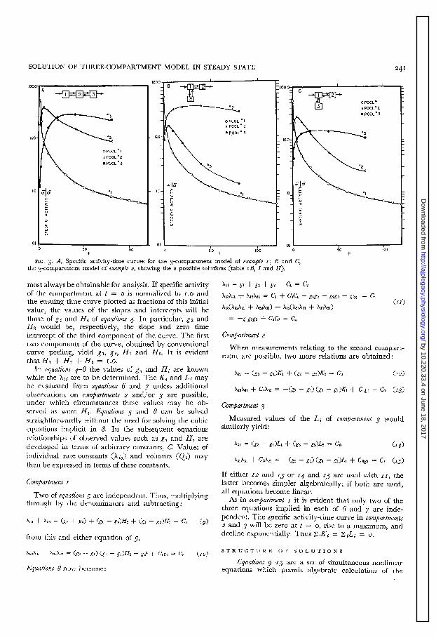
FIG. 3. A, Specific activity-time curves for the 3-compartment model of example I; I3 and C, the g-compartment model of example 2, showing the 2 possible solutions (table IB, I and 11).

most always be obtainable for analysis. I f specific activity of the compartment at t = o is normalized to 1.0 and the ensuing time curve plotted as fractions of this initial value, the values of the slopes and intercepts will be those of gi and Hi of equations 4. In particular, g3 and H3 would be, respectively, the slope and zero time intercept of the third component of the curve. The first two components of the curve, obtained by conventional curve peeling, yield g 1, g2, HI and Hz. It is evident that&+&+H3= 1.0.

In equations 4-8 the values of gi and Hi are known while the Xij are to be determined. The Ki and Li may be evaluated from equations 6 and 7 unless additional observations on compartments 2 and/or 3 are possible, under which circumstances these values may be .observed as were Hi. Equations 5 and 8 can be solved straightforwardly without the need for solving the cubic equations implicit in 8. In the subsequent equations relationships of observed values such as pi and Hi are developed in terms of arbitrary constants, C. Values of individual rate-constants (X& and volumes (Q;> may

then be expressed in terms of these constants.

Compartment 1

Two of equations 5 are independent. Thus, multiplying through by the denominators and subtracting:

X22 + x33 = (g2 + 93) + (91 - g2)H2 + (gl - g3)H3 = Cl (9)

from this and either equation of 5,

X22h - h&32 = (g2 - RI) (g2 - gs)rr, - g22 + c,g2 = c2 Go>

Equations 8 now become:

x11 = gr + g2 + g3 - Cl = c3

x13x31 + h2h21 = c2 + C3Cl - g1g2 - g2g3 - g3g1 = c4

&3@32~21 + h2~31) + h2(h23h31 + x33x21)

= -gig293 + c3c2 = cb

Compartment 2

When measurements relating to the second compartment are possible, two more relations are obtained:

x21 = (g 3 - gl)K; + (g3 - g2)K2 = c6 (4

h23h31 + c6h33 = - c? 2 - gl) (g3 - gl)K; + c,gI = c7 (13)

Comj.wrtment 3

Measured values of the Li of compurtment 3 would similarly yield :

X31 = (93 - g&l + (g3 - g2)L2 = C8 ( 4) I

x32x21 + c8x22 = - (g2 - g1) (g3 - gl)Ll + c8gl = c9 (15)

I f either r2 and 13 or 14 and r5 are used with or, the latter becomes simpler algebraically; if both are used, all equations become linear.

As in compartment I it is evident that only two of the three equations implied in each of 6 and 7 are independent. The specific activity-time curve in compartments 2 and 3 will be zero at t = o, rise to a maximum, and decline exponentially. Thus L:& = Z: & = o.

STRUCTURE OF SOLUTIONS

Equations g-15 are a set of simultaneous nonlinear equations which permit algebraic calculation of the


Dow

nloaded from


S. M. SKINNER, R. E. CLARK, N. BAKER AND R. A. SHIPLEY

I5 CI III1 r III 1 I

- Q3

IO

5

0

- -

- -

-

-

15

IO

i 5 II

P-- - 0.01 0.05

g2 0.1

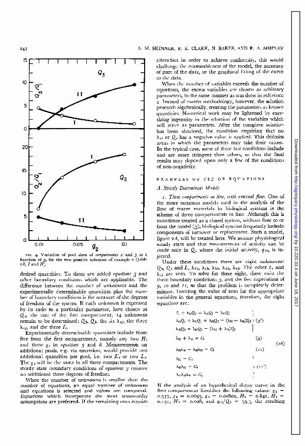
FIG. 4. Variation of pool sizes of compartments 2 and 3 as a function of g2 for the two possible solutions of example z (table I B, I and 11).

desired quantities. To them are added equafions 3 and other boundary conditions which are applicable. The difference between the number of unknowns and the experimentally determinable quantities plus the number of boundary conditions is the measure of the degrees of freedom of the system. If each unknown is expressed by its ratio to a particular parameter, here chosen as Qr, the size of the first compartment, 14 unknowns remain to be determined: Qs, Q3, the six X;j, the three X,i, and the three li.

Experimentally determinable quantities include those five from the first compartment, namely any two Hi and three gi in equations 5 and 6. Measurements on additional pools, e.g. via excretion, would provide two additional quantities per pool, i.e. two Ki or two Li. The gi will be the same in all three compartments. The steady state boundary conditions of equations 3 remove an additional three degrees of freedom.

When the number of unknowns is smaller than. the number of equations, an equal number of unknowns and equations is selected and values are computed. Equations which incorporate the most trustworthy assumptions are preferred. If the remaining ones require

alteration in order to achieve conformity, this would challenge the reasonableness of the model, the accuracy of part of the data, or the graphical fitting of the curve to the data.

When the number of variables exceeds the number of equations, the excess variables are chosen as arbitrary parameters, in the same manner as was done in reference 2. Instead of matrix methodology, however, the solution proceeds algebraically, treating the parameters as known quantities. Numerical work may be lightened by exer- cising ingenuity in the selection of the variables which will serve as parameters. After the complete solution has been obtained, the condition requiring that no Xij or Qi has a negative value is applied. This delimits areas in which the parameters may take their values. In the typical case, some of these last conditions include and are more stringent than others, so that the final results may depend upon only a few of the conditions of non-negativity.

EXAMPLES OF USE OF EQUATIONS

A. Strictly Determinate Models

I. Three comj.?artments in line, with external flow. One of the more common models used in the analysis of the flow of tracer materials in biological systems is the scheme of three compartments in line. Although this is sometimes treated as a closed system, without flow to or from the model (3), biological systems frequently include components of turnover or replacement. Such a model, figure 2A, will be treated here. We assume physiological steady state and that measurement of activity can be made only in Qr where the initial activity, q 10, is injected.

Under these conditions there are eight unknowns: Qz, Q3 and 11, X 21, X12, X23, X32, Xg3. The other Ji and Xii are zero. To solve for these eight, there exist the three boundary conditions 3, and the five expressions of 9, rb and II, so that the problem is completely determinate. Inserting the value of zero for the appropriate variables in the general equations, therefore, the eight equations are :

11 + xlzQ2’ = ~QI = X21Q1

X23(23 + X21Q1 = h22Q2 = (x12 + b)Q2 (3’)

x32Q2 = 133Q3 = (ha + bs>Q3

x22 + x33 = Cl

x22x33 - X23X32 = 472

x11 = c3

hh2 = cs

&2X33x21 = G 1 I f the analysis of an hypothetical decay curve in the first compartment furnishes the following values: gr = o*577, 92 = 0.0693, g3 = 0.00802, HI = 0.841, H2 = 0.131, Hs = 0.028, and qlo/Q1 = 53.5, the resulting


Dow

nloaded from



solution is shown in table r A. With certain modifica- tions of the general model a direct numerical substitu- tion in equations 3,9, 10 and I r may be simpler than the algebraic formulation of Xij and Qi in terms of the constants C.

Using the values (table ~4) of the variables, one may now compute the K’i and the Li, and therefore the time- wise course of specific activity in the second and third compartments. Figure 3A shows the specific activity in all three compartments semilogarithmically as a function of time.

2. One reserve compartment. The model used here is that of figure a& with 13 and X 03 equal to zero. In this case, the unknowns to be determined are:

With the same two assumptions as in the first example, the equations available for solving the model are:

11 + h3Qx + h2Q2 = X11Ql

x21Q1 = X22Q2

1

N (3 1

X31Q1 = x33Q3

x22 + x33 = Cl (9)

( 7) I &&3 = cz C~O3 x11 = (73

X31&3 + X21&2 = G I

I

(r I”)

h3~22h + h2x33x21 = GJ

As is evident from equations 9 and IO’, the solution will involve a quadratic, and two solutions may be possible:

x 22 = S(Cl zk -\/ciF32) = Cl0

x33 = $&l =I= z/c@=33 = Cl1

With the same values for the g; and Hi sohtz’ons I and 11 are obtained as shown in table IB. The & and the L,i may be computed and curves of specific activity drawn as shown in figures 3B and C. In this case, one must choose between the two solutions on some basis such as the reasonableness of pool sizes or rates as suggested by independent data. If the order of magnitude of any such additional criteria is known, decision between two solutions can be made even in the absence of exact values, since the choice is between solutions which themselves are mathematically explicit.

For example, if pool I in this hypothetical example is considered to be plasma, and pool 2, interstitial fluid (with the outflow h 02 indicating irreversible flow into cells), and if the material under study is known to penetrate readily through capillaries, the data of figure

gB might be eliminated in favor of that of figure 3C. Pool 2 (fig. 3B) is excessively large, and its specific activity-time curve is markedly divergent from that of pool r. Figure 4 indicates the variation in the size of compartments 2 and 3 as g 2 varies while g 1 and g3 remain fixed. This graphically predicts the uncertainty in Q2. and Q3 resulting from errors in estimate of g2.

t Eq. W W = 0.01516

Eq. W W=O.01176

W = 0.00862 3 -e

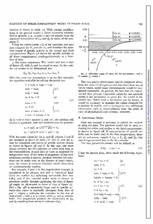
FIG. 5. Allowable range of values for the parameters v and w of exum$e 3, solution I.

The two strictly determinate models computed above from the same set of experimental data both show sets of values which, under many circumstances, would be considered reasonable. En general, the fact that the experimental data provide reasonable values for one assumed model is not acceptable as proof that the model is the correct one. Before such a conclusion can be drawn, it would be necessary to examine the values obtained for a number of models, and to incorporate any additional information such as reasonableness from the point of view of physiological and chemical processes.

B. Indeterminate Models

Only one example is necessary to exhibit the method of using the data. The previous model will be used, in- cluding the inflow and outflow at the third compartment, as shown in figure 2B. I f measurements of specific activity can be made only in the first compartment, there are I o unknowns, namely 6 Xii, 2 Ii, Q2 and Q3, but only 8 experimental data to fix the variables.

The two parameters chosen will be defined as

13/Q1 = v; x03 = w Cm

Using the known data, there result the following equations :

x22 + x33 = Cl (91 x22x33 = c2 (4

x11 = c3

X13X31 + h2X21 = c4 \

i

(I I")

h22h3h31 + h33h2h21 = c5

x21 + x31 = x11 I

&I2 + h2 = x22 I

I

c > I' ( 91 I

w -I- x13 = x33

11 + h2Q2 + h3Q3 = hQ1

x2iQ1 = X22Q2

I

(3’“)

(v + h)Ql = x33Q3


Dow

nloaded from


It may be noticed that the values of xii do not depend upon u or ZU. When C12, (713 are defined as (C&II - C,>/

CC 11 - GO), (G - GGo)/(CH - GO), respectively, one obtains the relationships shown below and in table IC.

xi-J3 = w 0 a

Is/Ql = ZJ w

x13 = Cl1 - w 0 C

x31 = cl2/h3 = h/(cll - w) (0

x21 = c3 - x31 = c3 - G2/CG - 4 0 e

x12 = cl3/h2l = cl3@& - w)Icc,(c,l - w> - Cl21 (f)

x02 = Go - Xl2 = Go - G3CGl - 4 (20)

C3Gl - w> - Cl2 (49

c

QdQl c3

= A&Tio = -- - Cl2

Go GOGl - 4 @I

Q3/Q1 = ‘+ = F + c (cc12 w> 0 i

11 1 11 11 -

Cl3 G2 Il/Ql = C3 - c - c - v 0 I-

10 11 ( > I - ;

11

To see how much variability in these quantities is introduced by permitting the flows X0 3 and 13, the values of the gi and Hi used in the last example are taken. In 20, a and b require that

v > 0, w 2 0. -

REFERENCES

I. ROBERTSON, J. S. Physiol. Rev. 37 : I 33, 1957. 2. BERMAN, M, AND R. SCHOENFELD. 3. A$J#. Phys. 27: II, 1956.

S. M. SKINNER, R. E. CLARK, N. BAKER AND R. A. SHIPLEY

Equation G requires that

w 5 0.01516, w < 0.1446

in which the values for the two alternate solutions, 1 and II, are shown. Equation d contributes nothing new, but equation G reduces the possible range of values to:

($ozzltion I) (~ozution II) v 2 o, o 5 w 5 0.01176 v > 0, 0 2 w < 0.07513.

Equation f again contributes nothing new, but equation g further reduces the range to:

v 2 o, o 5 w 2 0.008620 71 > o, o < w 2 0.05506

Equation h and i add nothing, but equation j contributes:

v I-- (

W

0.015162 > 2 0.1461 v(1 -5) so*1461

so that when tel = o,

o < v 5 0.1461 o 5 v 5 0.1461

and when w has its maximum value, in either case,

W = 0.008620, o 5 v 2 0.3387 w = 0.05506, o 5 u 5 0.2360

In figure 5, the possible values of u and zo resulting from solution I are plotted, and the regions eliminated by the various equations above are indicated. The numerical values for both solutions are given in table I C.

Analyses made in the fashion of the preceding examples provide explicit solutions for a great variety of flow problems. In cases such as example 3 above, where one or more degrees of freedom exist, one may investigate the sensitivity of any given variable (Qi, A ij, or r,> to changes in the parameters for which a range has been established.

3a ROBERTSON, J. S., D. C. TOSTESON AND J. L. GAMBLE. 3. Lub. & Clin. Med. 49: 497, 1957.


Dow

nloaded from


complete solution of the three-compartment model in … · solution of three-compartment model in...

Documents