completely recursive least squares and its applications
TRANSCRIPT

University of New OrleansScholarWorks@UNO
University of New Orleans Theses and Dissertations Dissertations and Theses
Summer 8-2-2012
Completely Recursive Least Squares and ItsApplicationsXiaomeng BianUniversity of New Orleans, [email protected]
Follow this and additional works at: https://scholarworks.uno.edu/td
Part of the Power and Energy Commons, and the Signal Processing Commons
This Dissertation is brought to you for free and open access by the Dissertations and Theses at ScholarWorks@UNO. It has been accepted for inclusionin University of New Orleans Theses and Dissertations by an authorized administrator of ScholarWorks@UNO. The author is solely responsible forensuring compliance with copyright. For more information, please contact [email protected].
Recommended CitationBian, Xiaomeng, "Completely Recursive Least Squares and Its Applications" (2012). University of New Orleans Theses and Dissertations.1518.https://scholarworks.uno.edu/td/1518
Completely Recursive Least Squares and Its Applications
A Dissertation
Submitted to the Graduate Faculty of the
University of New Orleans
in partial fulfillment of the
requirements for the degree of
Doctor of Philosophy
In
Engineering and Applied Science
Electrical Engineering
by
Xiaomeng Bian
B. S. Zhejiang University, China, 2000
August, 2012

ii
@Copyright 2012, Xiaomeng Bian

iii
Dedication
This dissertation is dedicated to all I have ever learnt from. Sincerely.

iv
Acknowledgement
First, I would like to give my sincere thanks to my families: my parents, uncles and aunties,
brothers and sisters, and my in-heaven grandparents. Their selfless love and firm support
encourage me to face all the challenges in my study-and-life time.
I would like to give my sincere thanks to Dr. George E. Ioup, Dr. Linxiong Li, Dr. Vesselin
P. Jilkov, Dr. Huimin Chen and Dr. Zhide Fang for the helpful guidance, suggestions and
comments, as well as the patience and time that you have provided. I would express my
gratitude to Professor Jiaju Qiu, Professor Deqiang Gan and Professor Meiqin Liu from
Zhejiang University, China. I do appreciate your kind instructions and encouragements in the
past years. I would also say special thanks to Dr. Huimin Chen for your insightful discussions
and comments on my papers and dissertation.
I would also like to express my gratitude to Dr. Ming Yang, Dr. Zhansheng Duan, Dr. Ryan
R. Pitre, Mr. Arther G Butz, Mr. Yu Liu, Mr. Rastin Rastgoufard, Mr. Jiande Wu, Mr. Gang
Liu, Dr. Bingjian Wang, Dr. Liping Yan, Miss Jing Hou and all the other colleagues and
classmates I have met. I do enjoy the “attacking” atmosphere in our Information & System Lab.
Your challenging questions do help me refine and improve my ideas.
Finally and foremost, I would like to thank my major advisor Dr. X. Rong Li for maturing
me academically and for teaching me the art of critical thinking [R. R. Piter]. It is because of
your strict and normative training and guidance that I can truly feel the beauty in the new
realm. Thank you.

v
Table of Contents
List of Figures .......................................................................................................................... viii
List of Tables .............................................................................................................................. ix
Abstract ....................................................................................................................................... x
1. Introduction and Literature Review .....................................................................................001
1.1 Classification of LS, WLS and GLS ..............................................................................001
1.2 Review of Batch LS/WLS/GLS Solutions.....................................................................002
1.2.1 Batch LS/WLS Methods .........................................................................................002
1.2.2 Batch GLS and LE-Constrained LS solutions ........................................................008
1.3 Recursive LS Approaches ..............................................................................................009
1.3.1 Recursive Methods..................................................................................................009
1.3.2 RLS Initialization and Deficient-Rank Problems ...................................................011
1.4 Completely Recursive Least Squares (CRLS) ...............................................................014
1.5 CRLS, LMMSE and KF.................................................................................................015
1.6 Power System State Estimation and Parameter Estimation ...........................................016
1.7 Our Work and Novelty ...................................................................................................017
1.8 Outline............................................................................................................................021
Nomenclature in Chapters 2-3 .................................................................................................022
2. Completely Recursive Least Squares—Part I: Unified Recursive Solutions to GLS..........024
2.1 Background ....................................................................................................................024
2.2 Problem Formulation .....................................................................................................026
2.3 Theoretical Support ........................................................................................................027
2.3.1 Preliminaries ...........................................................................................................027
2.3.2 Recursive solutions to unconstrained GLS .............................................................028
2.3.3 Recursive solutions to LE-constrained GLS ...........................................................031
2.3.4 Recursive imposition of LE constraints ..................................................................032
2.3.5 Recursive solution to coarse GLS ...........................................................................035
2.4 Unified Procedures and Algorithms .........................................................................................042
2.5 Performance analysis .....................................................................................................045
2.6 Appendix 046
2.6.1 Appendix A: Proof of Proposition 1........................................................................046
2.6.2 Appendix B: Proof of Theorem 1............................................................................047
2.6.3 Appendix C: Proof of Fact 4 ...................................................................................049
2.6.4 Appendix D: Proof of Theorem 2............................................................................050
2.6.5 Appendix E: Proof of Theorem 3 ............................................................................051
2.6.6 Appendix F: Proof of Proposition 2 ........................................................................053
2.6.7 Appendix G: Proof of Proposition 3........................................................................053
2.6.8 Appendix H: Proof of Theorem 5............................................................................054
3. Completely Recursive Least Squares—Part II: Recursive Initialization, Linear- Equality
vi
Imposition and Deficient-Rank Processing........................................................................055
3.1 Introduction ....................................................................................................................055
3.1.1 Background .............................................................................................................055
3.1.2 Our Work ................................................................................................................056
3.2 Problem Formulations....................................................................................................057
3.2.1 WLS and Its Batch Solutions ..................................................................................057
3.2.2 RLS Solutions .........................................................................................................059
3.2.3 Our Goals ................................................................................................................059
3.3 Derivations and Developments ......................................................................................060
3.3.1 Preliminaries ...........................................................................................................060
3.3.2 Development of Recursive Initialization ................................................................060
3.3.3 Deficient-Rank Processing......................................................................................068
3.4 Overall Algorithm and Implementation .........................................................................070
3.5 Performance Analysis.....................................................................................................072
3.6 Appendices .....................................................................................................................074
3.6.1 Appendix A: Proof of Theorem 2 ...........................................................................074
3.6.2 Appendix B: Proof of Theorem 5............................................................................076
3.6.3 Appendix C: Proof of Theorem 6............................................................................078
4. Linear Minimum Mean-Square Error Estimator and Unified Recursive GLS ....................079
4.1 Review of LMMSE Estimation and GLS ......................................................................079
4.1.1 LMMSE Estimator ..................................................................................................079
4.1.2 LMMSE Estimation Based on Linear Data Model .................................................080
4.2 Verification of Generic Optimal Kalman Filter .............................................................082
Nomenclature in Chapters 5-6 .................................................................................................087
5. Joint Estimation of State and Parameter with Synchrophasors—Part I: State Tracking .....088
5.1 Introduction ....................................................................................................................088
5.1.1 Background and Motivation....................................................................................088
5.1.2 Literature Review....................................................................................................089
5.1.3 Our Work.................................................................................................................089
5.2 Formulation and State-Space Models ............................................................................090
5.2.1 State Tracking with Uncertain Parameters ..............................................................091
5.2.2 Prediction Model for State Tracking.......................................................................091
5.2.3 Measurement Model of State Tracking...................................................................092
5.3 Adaptive Tracking of State.............................................................................................093
5.3.1 Basic Filter Conditioned on Correlation .................................................................093
5.3.2 Detection and Estimation of Abrupt Change in State .............................................095
5.4 Procedure and Performance Analysis.............................................................................096
5.4.1 Explanations on Prediction and Measurement Models...........................................096
5.4.2 Implementation Issues.............................................................................................098
5.4.3 On Observability, Bad-Data Processing and Accuracy ..........................................099
5.5 Comparative Experiments..............................................................................................100

vii
5.6 Conclusions ....................................................................................................................106
5.7 Appendices .....................................................................................................................106
5.7.1 Appendix A: Derivation of Filter on Correlated Errors and Noise .........................106
5.7.2 Appendix B: Derivation of Abrupt Change Estimation ..........................................109
6. Joint Estimation of State and Parameter with Synchrophasors—Part II: Para. Tracking ....111
6.1 Introduction ....................................................................................................................111
6.1.1 Previous Work .........................................................................................................111
6.1.2 Our Contributions....................................................................................................112
6.2 Parameter Estimation .....................................................................................................113
6.3 Formulation of Parameter Tracking ...............................................................................114
6.3.1 Prediction Model.....................................................................................................115
6.3.2 Measurement Model................................................................................................115
6.4 Tracking of Line Parameters ..........................................................................................116
6.4.1 Basic Filter ..............................................................................................................116
6.4.2 Adjustment of Transition Matrix ............................................................................118
6.5 Error Evolution and Correlation Calculation .................................................................119
6.6 Procedures and Performance Analysis...........................................................................122
6.6.1 Parameter Tracking and Overall Procedure ............................................................122
6.6.2 Accuracy and Complexity.......................................................................................122
6.6.3 A Practical Scheme .................................................................................................123
6.7 Simulations.....................................................................................................................124
6.7.1 Comparisons with Other Approaches .....................................................................124
6.7.2 Practical Two-Step Implementation of the Approach.............................................126
6.8 Conclusions ....................................................................................................................128
6.9 Appendix ........................................................................................................................128
7. Summary and Future Work ...................................................................................................130
References .................................................................................................................................133
Vita ............................................................................................................................................140

viii
List of Figures
Fig. 5.1 State tracking procedure with abrupt-change detection..............................................099
Fig. 5.2 Realistic 18-bus system ..............................................................................................101
Fig. 5.3 Comparison on effect of parameter uncertainty..........................................................103
Fig. 5.4 Comparison on effect of abrupt-state-change detection .............................................105
Fig. 5.5 Comparison with random-walk model .......................................................................105
Fig. 5.6 Comparison with forecasting model ...........................................................................106
Fig. 6.1 Joint state and parameter estimation procedure..........................................................123
Fig. 6.2 12-bus 500kV system..................................................................................................125
Fig. 6.3 Performance comparison with EKF............................................................................126
Fig. 6.4 Practical scheme based on 12-bus system ..................................................................127
Fig. 6.5 Practical scheme based on 12-bus system (zoomed in)..............................................128

ix
List of Tables
TABLE 5.1 Brach Parameter (18-Bus System) .......................................................................103
TABLE 5.2 RMSEs of First Experiment .................................................................................104
TABLE 5.3 RMSEs of Secon Experiment ...............................................................................104
TABLE 6.1 Parameters (Realistic System) ..............................................................................125

x
Abstract
The matrix-inversion-lemma based recursive least squares (RLS) approach is of a recursive
form and free of matrix inversion, and has excellent performance regarding computation and
memory in solving the classic least-squares (LS) problem. It is important to generalize RLS for
generalized LS (GLS) problem. It is also of value to develop an efficient initialization for any
RLS algorithm.
In Chapter 2, we develop a unified RLS procedure to solve the unconstrained/linear-equality
(LE) constrained GLS. We also show that the LE constraint is in essence a set of special
error-free observations and further consider the GLS with implicit LE constraint in
observations (ILE-constrained GLS).
Chapter 3 treats the RLS initialization-related issues, including rank check, a convenient
method to compute the involved matrix inverse/pseudoinverse, and resolution of
underdetermined systems. Based on auxiliary-observations, the RLS recursion can start from
the first real observation and possible LE constraints are also imposed recursively. The rank of
the system is checked implicitly. If the rank is deficient, a set of refined non-redundant
observations is determined alternatively.
In Chapter 4, base on [Li07], we show that the linear minimum mean square error (LMMSE)
estimator, as well as the optimal Kalman filter (KF) considering various correlations, can be
calculated from solving an equivalent GLS using the unified RLS.
In Chapters 5 & 6, an approach of joint state-and-parameter estimation (JSPE) in power
system monitored by synchrophasors is adopted, where the original nonlinear parameter
problem is reformulated as two loosely-coupled linear subproblems: state tracking and
parameter tracking. Chapter 5 deals with the state tracking which determines the voltages in
JSPE, where dynamic behavior of voltages under possible abrupt changes is studied. Chapter 6
focuses on the subproblem of parameter tracking in JSPE, where a new prediction model for
parameters with moving means is introduced. Adaptive filters are developed for the above two

xi
subproblems, respectively, and both filters are based on the optimal KF accounting for various
correlations. Simulations indicate that the proposed approach yields accurate parameter
estimates and improves the accuracy of the state estimation, compared with existing methods.

1
Chapter 1: Introduction and Literature Review
1.1 Classification of Linear LS, WLS and GLS
The principle of least squares (LS), which was first invented independently by a few
scientists and mathematicians such as C. F. Gauss, A. M. Legendre and R. Adrain
[Stigler86][Li07], is a classic and standard approach to obtaining the optimal solution of an
overdetermined system to minimize the sum of squared residuals.
The most popular and important interpretation of the LS approach is from the application in
data fitting. That is, the best fitting in the LS sense is to approximate a set of parameters
(estimands) such that the sum of squared residuals is minimized, where the residuals are
differences between the measured observation values and the corresponding fitted ones
[Wiki01]. In addition, the LS problem also has various names in different disciplines [Li07].
For instance, in some mathematical areas, LS may be treated as a special minimum l2-norm
problem [Bjorck96]. In statistics, it is also formulated as a probabilistic problem widely used
in regression analysis or correlation analysis [Freedman05] [Kleinbaum07]. In engineering, it
is a powerful tool adopted in parameter estimation, filtering, system identification, and so on
[Sorenson80] [Ba-Shalom01]. In particular, in the area of estimation, the LS formulation can
be derived from the maximum-likelihood (ML) criterion if the observation errors are normally
distributed. The LS estimator can also be treated as a moment estimator [Wiki01].
Roughly speaking, LS problems can be classified into linear and nonlinear cases, depending
on whether the involved observation quantities are linear functions of the estimand or not. It is
also well known that, with linearization techniques such as Gauss-Newton methods, a
nonlinear LS problem may be converted to linearized iterative refinements. This dissertation
focuses on linear LS solutions.
More generally, the object of the data fitting may be extended to minimize the sum of the
weighted residual squares, which leads to the definition of least squares with weights.
According to the features of their weighting matrices, linear LS problems with weights can be

2
largely categorized from the simple to the complex as LS, weighted LS (WLS), and
generalized LS (GLS), where linear-equality (LE) constraints may be imposed. Note that in
this dissertation the concept of WLS is limited to the case with a diagonal matrix while the
GLS has a non-diagonal weighting matrix [Amemiya85] [Greene00] [Wiki02]. In addition,
linear-inequality constraints may also be involved and can be treated as combinations of LE
constraints [Lawson95].
Note that in some statistics books, “weighted least squares” may be used for LS problems
with equal weights while those with distinguished weights are named generally- weighted least
squares. As the equally-weighted LS and the conventional LS has the same solution plus
mutually-proportional estimation-error covariances, we ignore their difference and follow the
convention in [Lawson95] [Bjorck96]: WLS is for LS with distinguished (not all-equal)
weights and GLS is for LS weighted by an arbitrary PD matrix.
In summary, we use the following LS/WLS categorizing list to present the LS solutions
from simplest to most complex problem setup:
� Unconstrained LS � LE-constrained LS
� Unconstrained/LE-constrained WLS
� Unconstrained GLS � LE-constrained GLS
� Implicitly-LE-constrained (ILE-constrained) GLS
We focus on the development of the recursive unconstrained/LE-constrained/
ILE-constrained LS/WLS/GLS solutions and the related initialization as well as deficient-rank
processing. The study starts from the conventional RLS and its exact initializations, which are
reviewed below.
1.2 Review of Batch LS/WLS/GLS Solutions
1.2.1 Batch LS/WLS Methods
As a classic minimization problem, the LS problem has been studied for more than two
centuries. Many methods and algorithms have been developed and well surveyed in the past.
Most commonly-recognized methods and algorithms are presented in well-known books, such

3
as [Lawson95] and [Bjorck96]. Among the exiting LS methods and topics, we will review
those issues related to our research in detail. Roughly speaking, the (unconstrained) linear LS
approach is to solve the following classic (unconstrained) linear LS problem:
ˆ arg min J=x
x (1.1a)
with1( ) ( ) ( ) ( )
M T T
m m m mmJ z H z H
== − − = − −∑ x x z Hx z Hx (1.1b)
where [ ]T
nx=x L L , [ ]T T
mH=H L L , and [ ]T
mz=z L L . n
x is the thn to-be-determined
quantity. mH and m
z are the coefficient (row vector) and value of the thm observation,
respectively, and M is the total observation number. Typically, x can be obtained via
normal-equation solution, QR-decomposition (of H ), Gauss elimination and so on. These
methods are reviewed as follows.
The solutions can come from solving the following normal equation:
ˆ( )T T=H H x H z (1.2a)
That is,
1 1
ˆ( )M MT T
m m m mm mH H H z
= ==∑ ∑x (1.2b)
Clearly, if and only if (iff) rank( ) N=H , (1.2b) has a unique solution and the batch solution is
1( )
ˆ
T
T
− =
=
C H H
x CH z (1.2c)
where estimation-error-covariance-like (EEC-like) matrix C is closely related to the covariance
of estimation errors in engineering applications. Matrix triangularization and diagonalization
techniques such as Cholesky decomposition (LLT
decomposition) can be used to decompose
TH H and thus compute C and x efficiently [Martin&Wilkinson65] [Passino98], where
the symmetric structure of TH H is advantageous. Several variants, as well as different ways to
sequencing the CD operations, were discussed in [George81]. Reference [Golub96] also shows
that LLT
decomposition and the QR decomposition method can lead to equal upper triangular
matrices if H has full column rank.

4
Actually, x can also be determined directly from the nonsymmetric linear equation =Hx z .
Gauss elimination with partial pivoting is used to solve =Hx z , and different
Gauss-elimination based methods are surveyed in [Nobel73]. Among the existing approaches,
the Peters-Wikinson method is a uniform one. It utilizes the LU factorization to reduce the
original LS problem to a simplified one with a lower triangular coefficient. Because the
solution is obtained from the triangularized coefficient and thus suffers less from rounding
error, this method is numerically more stable than those using the normal equation directly.
More popularly, the QR decomposition can be employed to decompose the observation
coefficient matrix into a product of an orthogonal square matrixQ and an upper triangular
matrix such that
0T
T T = H Q R (1.3)
where R is an upper triangular square matrix. Correspondingly, the observation-value
vector z is transformed into
1 2 T
T T = z Q z z% % (1.4)
Accordingly, the objective function in (1.1a) becomes as simple as
1 1 2 2( ) ( )T TJ = − − +z Rx z Rx z z% % % % (1.5)
Then x can be obtained conveniently by solving the following linear equation
1ˆ =Rx z% (1.6)
The solution can take advantage of the upper-triangular structure of R and can be obtained by
back substitution efficiently. Accordingly, the computational complexity of solving (1.6),
which is denoted by the number of the involved floating-point operations (flops), is only as
low as 2( )O N (order of 2N ). The computation accuracy is also high because the observation-
coefficient-matrix decomposition suffers little from rounding errors [Bjorck96] [Golub96].
Subsequently, the major work is on constructing appropriate orthogonal matrixQ . Many
classic methods have been utilized, such as Householder reflection, Givens rotation, and
classical or modified Gram-Schmidt [Horn85] [Press07] [Parlett00].
5
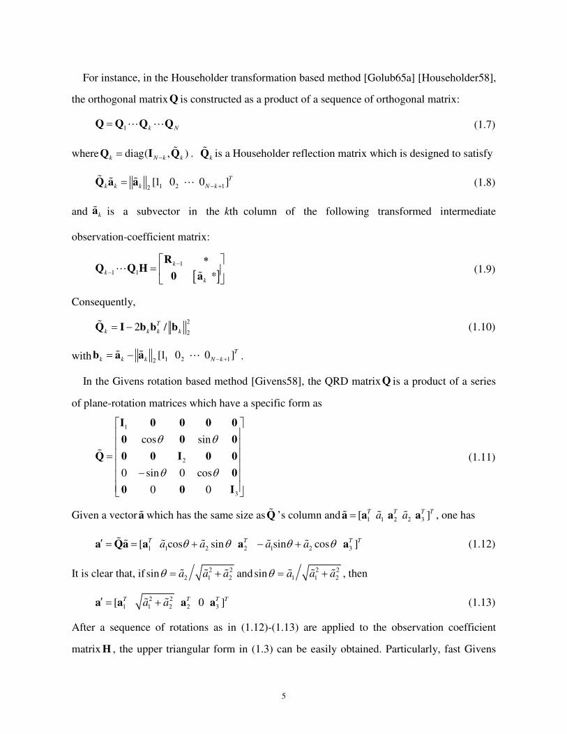
For instance, in the Householder transformation based method [Golub65a] [Householder58],
the orthogonal matrix Q is constructed as a product of a sequence of orthogonal matrix:
1 k N=Q Q Q QL L (1.7)
where diag( , )k N k k−=Q I Q% .
kQ% is a Householder reflection matrix which is designed to satisfy
1 2 12[1 0 0 ]T
k k k N k− +=Q a a% % % L (1.8)
and ka% is a subvector in the thk column of the following transformed intermediate
observation-coefficient matrix:
[ ]1
1 1 *
k
k
k
−−
∗ =
RQ Q H
0 aL
% (1.9)
Consequently,
2
22 /T
k k k k= −Q I b b b% (1.10)
with 1 2 12[1 0 0 ]T
k k k N k− += −b a a% % L .
In the Givens rotation based method [Givens58], the QRD matrixQ is a product of a series
of plane-rotation matrices which have a specific form as
1
2
3
cos sin
0 sin 0 cos
0 0
θ θ
θ θ
=
−
I 0 0 0 0
0 0 0
Q 0 0 I 0 0
0
0 0 I
% (1.11)
Given a vector a% which has the same size asQ% ’s column and 1 1 2 2 3[ ]T T T Ta a=a a a a% % % , one has
1 1 2 2 1 2 3[ cos sin sin cos ]T T T Ta a a aθ θ θ θ′ = = + − +a Qa a a a% % % % % % (1.12)
It is clear that, if 2 2
2 1 2sin a a aθ = +% % % and 2 2
1 1 2sin a a aθ = +% % % , then
2 2
1 1 2 2 3[ 0 ]T T T Ta a′ = +a a a a% % (1.13)
After a sequence of rotations as in (1.12)-(1.13) are applied to the observation coefficient
matrix H , the upper triangular form in (1.3) can be easily obtained. Particularly, fast Givens
6
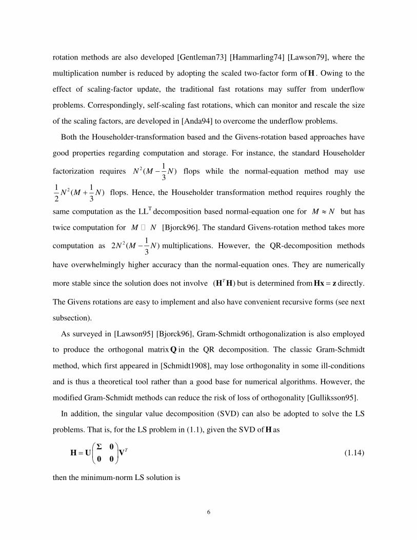
rotation methods are also developed [Gentleman73] [Hammarling74] [Lawson79], where the
multiplication number is reduced by adopting the scaled two-factor form of H . Owing to the
effect of scaling-factor update, the traditional fast rotations may suffer from underflow
problems. Correspondingly, self-scaling fast rotations, which can monitor and rescale the size
of the scaling factors, are developed in [Anda94] to overcome the underflow problems.
Both the Householder-transformation based and the Givens-rotation based approaches have
good properties regarding computation and storage. For instance, the standard Householder
factorization requires 2 1( )
3N M N− flops while the normal-equation method may use
21 1( )
2 3N M N+ flops. Hence, the Householder transformation method requires roughly the
same computation as the LLT
decomposition based normal-equation one for M N≈ but has
twice computation for M N� [Bjorck96]. The standard Givens-rotation method takes more
computation as 2 12 ( )
3N M N− multiplications. However, the QR-decomposition methods
have overwhelmingly higher accuracy than the normal-equation ones. They are numerically
more stable since the solution does not involve ( )TH H but is determined from =Hx z directly.
The Givens rotations are easy to implement and also have convenient recursive forms (see next
subsection).
As surveyed in [Lawson95] [Bjorck96], Gram-Schmidt orthogonalization is also employed
to produce the orthogonal matrix Q in the QR decomposition. The classic Gram-Schmidt
method, which first appeared in [Schmidt1908], may lose orthogonality in some ill-conditions
and is thus a theoretical tool rather than a good base for numerical algorithms. However, the
modified Gram-Schmidt methods can reduce the risk of loss of orthogonality [Gulliksson95].
In addition, the singular value decomposition (SVD) can also be adopted to solve the LS
problems. That is, for the LS problem in (1.1), given the SVD of H as
T =
Σ 0H U V
0 0 (1.14)
then the minimum-norm LS solution is

7
1 0
ˆ0 0
T
−+
= =
Σx H z V U z (1.15)
where superscript “+” stands for the Moore-Penrose pseudo inverse (MP inverse).
H1diag( , , )N
σ σ=Σ L , i
σ is the square root of the thi eignvalue of TH H , and Hrank( ) N=H .
The left and right singular vectors, which are stored in the orthogonal matrices U and V , are
the corresponding eignvectors of TH H and THH , respectively [Lawson95]. The first stable
algorithm based on SVD was presented in [Golub65b], where H is reduced to a bidiagonal
matrix via Householder transformation of a Lanczos process such that the singular values and
vectors refer to eignvalues and eignvectors of a special tridiagonal matrix [Bjorck96]. Later,
adaptation and improvement are made to the QR algorithm [Golub68] [Golub70]. Newer
Jacobi methods are also developed to improve the relative computation accuracy of the
singular values in bidiagonal matrices [Kogbetliantz55] [Hestenes58]. Note that, in (1.14),
HN N≤ . If HN N< , the SVD based solution leads to the minimum-norm LS solution, which is
a powerful tool for the deficient-rank analysis discussed in Sec. 1.3.2.
WLS is generalized from LS, in which each observation is assigned a positive weight:
ˆ arg min J=x
x (1.16)
with1( ) ( ) ( ) ( )
M T T
m m m m mmJ z H w z H
== − − = − −∑ x x z Hx W z Hx (1.17a)
Equivalently, ( ) ( )TJ = − −z Hx W z Hx , (1.17b)
where diag( , , )m
w=W L L (1.17c)
Theoretically speaking, sincem
w can be easily decomposed into1 12 2
m mw w , problem (1.16) can be
converted to an equivalent LS one without difficulty. As a result, all the batch LS methods,
such as the normal-equation based, the QRD based and the SVD based algorithms, are
applicable. The major issues arise from possible ill conditions deteriorated by significantly
large weight ratios and special efforts are made to treat the extremely ill-conditioned situations
[Vavasis94] [Hough94] [Bjorck80] [Duff94] [Gulliksson92] [Gulliksson95] [Anda94].

8
1.2.2 Batch GLS and LE-Constrained LS Solutions
Compared with WLS, GLS is a further generalized LS problem, where the weight W can
be an arbitrary positive definite (PD) matrix. Since a GLS problem can always be converted to
an equivalent LS form by decomposing W , those methods used for solving LS are all
applicable to GLS. For instance, the normal equation of GLS is
ˆ( )T T=H WH x H Wz (1.18)
where ( )TH WH remains symmetric. Then those normal-equation based methods used in LS,
such as LLT
decomposition based ones, can still be utilized.
Methods based on the decomposition of W are also widely adopted. That is,
T=W WW% % (1.19)
Based on (1.19), generalized QRD and SVD methods are developed, where the subsequent
decompositions of H and W% are performed separately to achieve better numerical accuracy
[Paige90] [Van76]. References [Anderson91], [De92] and [Paige81] further discuss the
implementation, application and extension of these generalized methods. In addition, how to
decompose W into the symmetric form (1.19) is also an issue. In principle, W% can be the
square root of W , which is unique since W is PD. The square root can be obtained by
orthogonal decomposition, Jordan decomposition, Denman-Beavers iteration, the Babylonian
method and so on [Higham86]. Particularly, W% can also be a lower triangular matrix.
Choleksy decomposition can be used. The computation can utilize W% ’s triangular structure.
In addition, in practical applications, constraints may be imposed to the LS solutions. For
example, in curve fitting, inequality constraints related to monotonicity, nonnegativety, and
convexity and equality constraints related to continuity and smoothness may be involved
[Zhu&Li07]. In the category of linear LS, linear-equality (LE) constrained problems are
widely investigated, in which problem (1.1) is subject to a set of consistent LE constraints as
=Ax B (1.20)

9
with AN N×∈A � and (without loss of generality) Arank( ) N=A . One natural way to handle
the LE-constrained LS is direct elimination, with which x is reduced to a lower dimensional
vector since the constraints imply that AN components of x are always linear combinations of
the left AN N− . Correspondingly, the original problem is then converted to an unconstrained
LS problem with reduced dimensions equivalently [Bjorck67] [Lawson95]. The most popular
practical methods to solve LE-constrained problems are based on the introduction of Lagrange
multiplier [Chong07]. The weighting method is also widely adopted, where each LE constraint
is treated as an observation with a “huge” weight [Anda96]. Although this method is very easy
to implement, it may lead to poor numerical condition. The LE-constrained LS solution can
also be obtained using the null-space method [Leringe70], based on which the close form of
the solution can be:
ˆ [ ( )] ( )B+ + + += + − −x A H I A A z HA B (1.21)
where +A stands for the Moore Penrose generalized inverse of A . If rank([ ] )T T T N=A H ,
(1.21) is the unique solution; otherwise, (1.21) leads to the minimum-norm solution in
rank-deficient problems [Wei92a] [Wei92b]. [Zhu&Li07] gives another null-space based form
as in (24), which is a useful tool for the subsequent derivations in this dissertation. In addition,
other techniques, such as the generalized SVD [Van85], are also introduced to solve and
analyze the LE-constrained LS problem. In this dissertation, our purpose is to develop
completely recursive LS which provides solutions (theoretically) identical to the batch ones.
The above batch methods will provide a solid foundation for the subsequent development.
1.3 Recursive Approaches
1.3.1 Recursive Methods
The above batch methods, such as QRD, SVD and normal-equation methods, can be
implemented recursively [Apolinario09]. That is, the current solution can be obtained by
updating the previously-processed one (using old observation data) with new observations.
10
In those observation-coefficient-matrix decomposition based methods, recursive procedures
mainly aim to construct the orthogonal matrix Q recursively [Gill74]. For instance, in the
Givens-rotation QRD methods, the rotations of the new observation coefficient can naturally
take advantage of the existing upper triangular matrix, where the computation complexity is at
2( )O N per cycle [Yang92]. The Gram-Schmidt decomposition can also be performed
recursively in a stable way with ( )O MN per-cycle computational operations [Daniel76]. The
recursion is still applicable to SVD, but the updating computation requires 2( )O MN flops at
each cycle [Bunch78], which is too much compared with recursive Givens rotation and
Gram-Schmidt orthogonalization.
Particularly, the matrix-inversion (MI) lemma based RLS, which is a recursive
normal-equation method, can obtain C (and x ) in another sequential way [Woodbury50]
[Chen85]. We will further investigate the MI-lemma-based RLS and generalize it to solve GLS
problems. The proposed recursive GLS (RGLS) techniques are also applicable to the
QRD-RLS.
Concretely, initialized by
0
0 0 0
1
1( ) ( )
M T T
M m m M MmH H
−′ ′′=
= =∑C H H (1.22)
the EEC-like matrix C of the unconstrained LS problem (1.2c) can be computed exactly by the
following recursion cycle:
1
1 1 1 1( 1)T T
m m m m m m m m mH H H H
−− − − −= − +C C C C C (1.23)
where 0M is the number of initial observations and the recursion/data index 0m M> . ˆm
x can
be calculated concurrently.
Furthermore, when a set of consistent LE constraints as in (1.20) is imposed, the unique
solution exists iff rank([ ] )T T T N=A H :
1
1[ ( ) ]
ˆ ( )
MT T T
m mm
T
H H−
=
+ +
=
= + −
∑C U U U U
x A B CH z HA B (1.24)

11
where 1[ ]T T T
M MH H= =H H L , 1[ ]T
M Mz z= =z z L , U satisfies [ ][ ]T =U U U U I% % and
col( ) col( )T=U A% [Zhu&Li07]. Here “ col( )X ” denotes the space spanned by all the columns
of X . Reference [Zhu&Li07] also shows that, the recursion formula in (1.23) is still applicable
for the LE case once the LE constraint (1.20) has been imposed on the initialization
appropriately. For instance, the recursion procedure for the EEC-like matrix should be
initialized as
0
0
1
1[ ( ) ]
MT T T
M m mmH H
−′ ′′=
= ∑C U U U U (1.25)
where the iff condition 0
rank([ ] )T T T
M N=A H is implicitly satisfied.
In addition, fast RLS methods are also developed [Ljung78] [Cioffi84], where the
computation is reduced from some convenient properties of the data, such as the involved
matrices’ Toeplitz structure.
The RLS is particularly suitable for real-time applications since sequential algebraic
operations at each cycle require low computation as well as fixed storage [Zhou02]. It has been
widely applied to such areas as signal processing, control and communication [Mikeles07]. In
adaptive-filtering applications, “RLS algorithms” are even referred in particular to RLS-based
algorithms for problems with fading-memory weights [Haykin01]. As a normal-equation
method, a major disadvantage of the RLS methods is that they have relatively poor numerical
stability (for getting x ), compared with direct observation-function coefficient factorization
methods. Fortunately, recursive QRD methods, such as Givens rotations, can be combined to
improve numerical stability [Proudler88] [Cioffi90a] [Cioffi90b] [Li07].
1.3.2 RLS Initialization and Deficient-Rank Problems
In the MI-lemma based RLS, to guarantee that the LS solutions at each recursion cycle are
identical to the corresponding batch ones, the procedure needs to start from an exact LS
initialization, which leads to the RLS initialization problem. However, although RLS has been
well studied and applied in the past decades, less attention has been paid to the RLS
initialization. It is because RLS is mainly applied to low-dimensional and high-redundancy

12
problems in areas such as signal processing, where the calculations for the batch LS solutions
based on a small number of initial observations may not be so costly in quite a few cases.
However, a simple initialization is still desired. In the original work, the following
approximation is adopted [Albert65]:
1
0
0ˆ
α − =
=
C I
x 0 (1.26)
whereα is a tiny positive number. With (1.26), the recursion (1.23) for the unconstrained RLS
can start from the first piece of observation data. It is clear that the recursion initialized by
(1.26) leads to the exact LS solution iff 0α → . Although it is hard to implement such
an 1α − exactly, (1.26) is widely adopted where the effect of the approximate α may be trivial
when observations keep accumulating. However, in some practical applications, the negative
effect caused by 0α ≠ may not be ignored and a too small α may deteriorate numerical
conditions. In [Hubing91], an exact initialization scheme is studied, which makes full use of
the special form of the initial observations in recursion-based adaptive filtering:
0
0
0
=
xM
M,
1
1
0
x =
xM
M,
2
1
20
x
x
=
x
M
, L , 1
1
N
N
N
x
x
x
−
=
xM
(1.27)
Furthermore, recursive QR-decomposition methods can also be used to transform the
coefficient matrix of initial observations into the upper triangular form, based on which the
initialization is recursive and easier to be determined [Haykin01]. Reference [Zhou02]
introduces variants of the Greville formula (order recursion) to develop recursive
initializations for RLS, where the recursion can also start from the first piece of data. We will
study a simple recursive exact RLS initialization method using the RLS formulae. We will also
apply the newly-developed method to solve high-dimensional and low-redundancy problems
such as power system state estimation, where recursive initialization does play an important
role in solving the LS state estimation problems. In addition, two accessorial issues should also
be studied. One is whether and when the foregoing observations can support an exact and

13
unique RLS initialization, namely (parameter) observability analysis (or rank check) in
engineering. In previous work, observability analysis usually requires extra numerical or
topological analysis [Chan87] [Chan94] [Monticelli00]. Correspondingly, if all the
observations can not uniquely determine a LS solution, then it leads to deficient-rank LS
problems. There are two possible deficient-rank situations: (a) there are no sufficient
observations, so that some to- be-determined quantities can not be uniquely determined (or the
estimand is unobservable); (b) although the observations are sufficient in theory, the estimand
is numerically unobservable due to ill conditions caused by round-off error, e.g., the involved
matrix inverses exist in theory but can not be computed numerically. The first situation is
theoretical rank deficiency while the second one is numerical rank deficiency [Stewart84]. In
addition, the other ill-conditioned case is also treated as numerical rank deficiency, in which
the observations are not sufficient in theory but still make the estimand observable due to the
effect of round-off error. Topological analysis can detect theoretical deficiency of observations
[Monticelli00] while numerical analysis can disclose the implementation details. The latter is
well investigated in the past. For instance, SVD based method is used to determine the
numerical rank of a matrix, where the singular values in Σ reveal the numerical condition of
the LS problem [Manteuffel81]. Cholesky decomposition and QRD methods, such as
Householder transformation, Givens rotation and modified Gram-Schmidt orthogonalizations,
are also used to examine the numerical rank of the LS problem, where column pivoting is
widely used [Golub65a]. Among these decomposition based methods, the SVD is the most
reliable one to reveal the matrix rank in general [Bjorck96]. Once numerical rank deficiency is
detected, caution has to be taken to fix or avoid this ill-conditioned situation [Dongarra79].
The second issue is how to handle problems with theoretically insufficient observations.
Note that, at this stage, the concepts of solving LS problem and performing LS estimation are
different. For a deficient-rank LS problem, there exist infinitely many feasible solutions to
minimize the squared sum, among which the one having the minimum norm and a simple
analytical form in batch is widely adopted [Lawson95] [Zhou02]. However, for LS estimation,

14
a deficient-rank situation means the estimand is not observable and no estimate exists. We
treat the deficient-rank problem from the viewpoint of LS estimation and introduce a
reduced-dimensional alternative estimate which is observable and has specific physical
interpretations.
1.4 Completely Recursive Least Squares (CRLS)
The RLS is originally applied to solve unconstrained LS problems [Albert65]. Recently,
[Zhu&Li07] found that the exact solution of LE-constrained LS can be obtained by the same
recursion as for the unconstrained problem, provided that the RLS procedure is appropriately
initialized. Owing to the excellent performance of the RLS regarding efficient real-time
computation and low memory, it is worthwhile to apply the RLS techniques to perform the
initialization of RLS recursively. It is also of value to generalize the conventional RLS as well
as the corresponding recursive initialization method and develop an integrated solution for
LE-constrained GLS problems. Consequently, there are two major issues worth studing. The
first issue is how to generalize the RLS method and solve the WLS and GLS problems in
similar recursive/sequential ways. It is clear that the square-root values of the diagonal
elements of the diagonal weighting matrix in the WLS can be simply multiplied into the
coefficient matrices. The WLS problem is thus converted to an LS one. In other words, a
recursive WLS (RWLS) method can be developed from the RLS easily. Therefore, the major
focus will be on the development of the recursive GLS (RGLS). The second issue is a
recursive initialization applicable to all the RLS, RWLS and RGLS. Actually, in the
RLS/RWLS and the newly-developed RGLS, the determination of exact solutions relies on
appropriate initializations. We will study a simpler recursive initialization method for the
RGLS as well as the RLS/RWLS, which is still based on the RLS formulae. In brief, with such
a generalized RLS approach, the recursion can start from the first piece of data no matter what
dependence the newly-arriving data have on the old data. The recursion can also be
implemented for both unconstrained and explicitly/implicitly LE-constrained cases. In these
senses, the newly-developed approach is named Completely Recursive Least Squares (CRLS).

15
1.5 CRLS, LMMSE and KF
In statistics and signal processing, the widely-used linear minimum mean-square error
(LMMSE) estimator is a linear function, in fact, an affine function of the observation that
achieves the smallest means-square error among all linear/affine estimators [Johnson04].
LMMSE estimator is the theoretical fundament of linear filtering: Kalman filtering, LMMSE
filtering (for nonlinear problems), (steady-state) Wiener filtering, and so on [Li07].
As is known in [Li07] that, given a linear data model, an LMMSE estimator with
complete/partial prior knowledge (i.e., prior mean, prior covariance and the cross- covariance
between the random estimand and the measurement noise) can always be treated as the
LMMSE estimator without prior information by unifying the prior mean as extra data. It is also
true that a linear-data-model-based LMMSE estimator without prior knowledge may be a
unification of Bayesian and classic linear estimation [Li07]. In other words, a
linear-data-model-based LMMSE estimator for a random estimand may be mathematically
identical to a linear WLS/GLS estimator using the PD joint covariance of the estimand and the
measurement noise as the weight inverse. In addition, the GLS with a positive semi-definite
(PSD) observation-error-covariance like (OEC-like) matrix has not been well posed, although
the LMMSE estimator with PSD measurement-noise covariance has been studied. We will
convert the LS with a PSD OEC-like matrix to an LE constrained GLS with implicit constraint.
As a result, the linear-data-model-based LMMSE estimation with a PSD measurement-noise
covariance, or more generally, the linear-data-model-based LMMSE estimator with a unified
PSD joint covariance of the estimand and the measurement noise can also be obtained by
solving the corresponding LS problems.
Furthermore, in the Kalman filter applied to linear systems with linear measurements, the
prediction is from an LMMSE estimator using the data up to the most recent time while the
update can be implemented from another LMMSE estimator using all the data up to the current
time. Owing to the mathematical equivalence between the linear-data-model based LMMSE
(without prior and with PD measurement error covariance) estimator and the GLS, the CRLS

16
can be applied to:
1) Verify the optimal Kalman filter accounting for the correlation between the prediction
error and the measurement noise, which was first derived in the LMMSE sense [Li07].
2) Apply the CRLS to improve the sequential data-processing scheme for the optimal
Kalman filter and to deal with various complicated situations caused by data correlation, PSD
covariance, etc.
Furthermore, we will apply the correlation-accounting KF to develop a series of adaptive
filtering techniques and to solve practical problems such as power system state estimation and
parameter estimation.
1.6 Power System State Estimation and Parameter Estimation
Power system state estimation, introduced to power systems in 1960s [Schweppe69], is to
estimate the involved bus voltages of a power system under steady-state conditions using
real-time voltage/power/current data collected by the supervisor control and data acquisition
(SCADA) system, where the steady-state system is usually modeled as a single-frequency,
balanced and symmetric one and the measured quantities, such as voltage magnitude,
active/reactive branch flow and active/reactive injection power, are all linear/nonlinear
functions of the bus voltages (system state) [Monticelli00] [Meliopoulos01]. Most of the
existing power system state estimation (SE) programs are formulated as static WLS problems
with one-scan data [Monticelli00]. Dynamic state estimation (DSE) is not popularly applied
due to practical limitations such as the complexity of measurement system and the inaccuracy
of dynamic and measurement models. Parameter estimation (PE) is responsible for calibrating
the suspicious measurement model parameters [Abur04], within which the bus voltages of
interest and the unknown parameters are usually stacked as an augmented state [Zarco00].
Correspondingly, dynamic-estimation methods are preferred since they exploit data from
multiple scans and take advantage of dynamic models [Leite87]. Unfortunately, similar
obstacles as in the DSE for bus voltages are encountered and the estimation accuracy is not
guaranteed. These dilemmas can be avoided in power systems metered by synchrophasors.

17
The invention of synchrophasor, also known as synchronized phasor measurement unit
(PMU), has led a revolution in SE since it yields linear measurement functions as well as
accurate data within three to five cycles [Phadke93]. In spite of the involved instrumental
channel errors [Sakis07] and the high cost, PMU has been tentatively used in centralized or
distributed estimators [Phake86] [Zhao05] [Jiang07] and in bad-data detection [Chen06].
We aim at performing accurate parameter and state estimation in complex situations using
synchrophasor data. An approach of joint state-and-parameter estimation, which is different
from the state augmentation, is adopted, where the original nonlinear PE problem is
reformulated as two loosely-coupled linear subproblems: state tracking and parameter tracking.
First, as a result of the reformulation, the state tracking with possible abrupt voltage changes
and correlated prediction-measurement errors is investigated, which can be applied to
determine the voltages in a PE problem or to estimate the system state in a conventional DSE
problem. Second, the parameter calibration of transmission network is also studied. For this
high-dimension low-redundancy nonlinear parameter estimation, we propose a balanced
method which adopts merits from both the extended Kalman filter (EKF) and the particle filter
(PF). It follows the simple structure of EKF but further accounts for the uncertain effects such
as involved bus voltages and high-order terms (of Taylor’s expansion) in EKF as pseudo
measurement errors correlated with prediction errors. Correspondingly, the recently-developed
optimal filtering technique that can handle correlation is introduced. We also introduce random
samples from the idea of PF to evolve the pseudo-error ensembles and to evaluate the statistics
related to the pseudo errors, where the error-ensemble sampling does not rely on the
measurement redundancy and is much easier to implement than PF. Based on this balanced
method, the joint state-and-parameter estimation considering complicated behavior of voltages
and parameters is discussed.
1.7 Our Work and Novelties
As reviewed in Sec. 1.3, the RLS is of a recursive form and free of matrix inversion, and
thus is excellent regarding efficient real-time computation and low memory. It is worthwhile to
18
generalize the above RLS procedure and to solve the unconstrained/LE-constrained GLS
problem in a similar recursive way. It is also of value to apply the RLS method for all the
involved RLS initializations. Consequently, the work of this dissertation includes: 1) to extend
the use of conventional to solve GLS problems in a similar recursive way; 2) to find efficient
recursive methods to initialize the RLS as well as the newly-developed recursive GLS
procedures; 3) to use the unified recursive GLS to improve the corresponding
sequential-data-processing procedures of the optimal KF considering various correlations; 4)
to exploit correlation-accounting KF based adaptive filtering approaches to perform power
system state estimation with synchrophasor measurements and treat parameter calibration of
the transmission network.
The generalization of the RLS for solving GLS problems is discussed in Chapter 2. Starting
from the unconstrained/LE-constrained RLS, we will develop a recursive procedure to solve
the unconstrained GLS, develop a similar recursive procedure applicable to the LE-constrained
GLS, and show that the LE constraint is in essence a set of special observations free of
observation errors and can be processed sequentially in any place in the data sequence. More
generally, we will consider recursive ILE-constrained GLS. A unified recursive procedure is
developed, which is applicable to ILE-constrained GLS as well as all the
unconstrained/LE-constrained LS/WLS/GLS.
In Chapter 3, a recursive exact initialization applicable to all the RLS, RWLS and RGLS, is
investigated. This chapter treats the RLS initialization-related issues, including rank check, a
convenient method to compute the involved matrix inverse/pseudoinverse, and resolution of
underdetermined systems. No extra non-RLS formula but an auxiliary-observation based
procedure is utilized. The RLS recursion can start from the first real observation and possible
LE constraints are also imposed recursively/sequentially. The rank of the system is checked
implicitly. If the rank is full, the initialization and the subsequent RLS cycles can be integrated
as a whole to yield exact LS estimates. If the rank is deficient, the procedure provides a
mapping from the unobservable (original) estimand to a reduced-dimensional set of alternative
19
quantities which are linear combinations of the original quantities and uniquely determined.
The consequent estimate is a set of refined non-redundant observations. The refinement is
lossless in the WLS sense: if new observations are available later, it can take the role of the
original data in the recalculation.
As shown in [Li07], the linear-data-model based linear minimum-mean-square-error
(LMMSE) estimator without prior with PD measurement-error covariance is mathematically
equivalent to the LS problem weighted by the measurement-error covariance. In Chapter 4, we
show that the linear-data-model based linear minimum-mean- square-error (LMMSE)
estimator can always be calculated from solving a unified ILE-constrained GLS. Consequently,
the recursive GLS can be used to improve the sequential procedure of the optimal KF
considering various correlations.
In Chapters 5 & 6, we aim at performing accurate parameter (and state) estimation in
complex situations using synchrophasor data, based on the optimal KF accounting for the
correlation between the measurement noise and the prediction error. An approach of joint
state-and-parameter estimation, which is different from the state augmentation, is adopted,
where the original nonlinear PE problem is reformulated as two loosely-coupled linear
subproblems: state tracking and parameter tracking, respectively.
Chapter 5 focuses on the state tracking, which can be used to determine bus voltages in
parameter estimation or to track the system state (dynamic state estimation). Dynamic
behavior of bus voltages under possible abrupt changes is studied, using a novel and accurate
prediction model. The measurement model is also improved. An adaptive filter based on
optimal tracking with correlated prediction-measurement errors, including the module for
abrupt-change detection and estimation, is developed. With the above settings, accurate
solutions are obtained.
In Chapter 6, we study the parameter tracking and the techniques dealing with the coupling.
A new prediction model for parameters with moving means is adopted. The uncertainty in the
voltages is covered by pseudo measurement errors resulting in prediction-measurement-error

20
correlation. An error-ensemble-evolution method is proposed to evaluate the correlation. An
adaptive filter based on the optimal filtering with the evaluated correlation is developed, where
a sliding-window method is used to detect and adapt the moving tendency of parameters.
Simulations indicate that the proposed approach yields accurate parameter estimates and
improves the accuracy of the state estimation, compared with existing methods.
In brief, our contributions include:
1) Combining RLS formulae with a recursive decorrelation method and developing a recursive
procedure for GLS;
2) Showing that an LE constraint is in essence a special observation free of error and can be
processed using RLS formulae at any place in the observation sequence;
3) Developing a unified recursive GLS procedure which is also used for ILE-constrained GLS;
4) Designing a simple auxiliary observation based RLS initialization procedure which allows
the recursion to start from the first piece of real observation data, where no extra technique
but the RLS formulae is used;
5) Inventing a new method to handle a deficient-rank LS problem, with which a set of
reduced-dimensional alternative estimates is provided for practical use;
6) When introducing the optimal KF accounting for prediction-measurement-error correlation
to solve joint state and parameter estimation in power systems monitored by synchrophasors,
we separate the original nonlinear problem as two coupled linear subproblems of state
tracking and parameter tracking.
7) In state tracking, we propose a new pair of prediction model and measurement model;
Develop a filtering method which can also detect the abrupt change; develop a new adaptive
filtering algorithm based on optimal tracking with correlated prediction-measurement errors,
including the module for the abrupt-change detection.
8) In parameter tracking, a new prediction model accounting for the effect of prior knowledge
and moving parameter means is proposed; a new adaptive filter is developed, based on the
optimal filtering with correlated prediction-measurement errors; a sliding-window method is

21
proposed to detect the moving tendency of parameters and adjust the transition matrix
adaptively; a sample-based method, namely, error-ensemble evolution, is used to evaluate
the correlation between pseudo measurement errors and prediction errors.
1.8 Outline
The rest of the dissertation is organized as follows. In Chapter 2, for the first part of the
CRLS approach, we will investigate the unified recursive GLS. The second part of CRLS,
which is on the exact recursive initialization and deficient-rank processing, is presented in
Chapter 3. In Chapter 4, the CRLS is then applied to verify the optimal KF (based on the
LMMSE criterion) which can handle the correlation between the prediction error and the
measurement noise. In Chapters 5 and 6, the correlation-accounting KF is applied to develop a
series of nonlinear filtering techniques to solve the problem of joint state and parameter
estimation in power systems metered by synchrophasors, where the original joint problem is
divided into two coupled subproblems as state tracking and parameter tracking.

22
Nomenclature in Chapters 2-3
The major notations used in Chapters 2 and 3 are listed below for quick reference.
i. Variables and Numbers
C estimation-error-covariance like (EEC-like) matrix
H (observation) coefficient (vector) in real-observation function
H (observation) coefficient (matrix) and mH
=
H
M
M
R observation-error-covariance-like (OEC-like) matrix; weight inverse if PSD
x estimand, full-/reduced-dimensional vector of to-be-determined quantities
z observation
z observation vector containing all z ’s
M total number of observations
N dimension of the estimand, row number of x
T total number of constraints
ii. Overlines
Let X be an original vector/matrix, then
X estimated X
X(
augmentation from X
X% temporarily-used quantities
X ′ after an LRC decorrelation
X ′′ related to the maximum-rank PD principal minor
DX used in an LRC decorrelation
X ∗ related to observations excluding implicit constraints

23
X o related to implicit LE constraints
iii. Subscripts and Indices
au of auxiliary observations
b of the (selected) basis of the row space of H(
lec linear-equality constrained
left of the left (undeleted) auxiliary observations
sim of a simple basis mapping x to an simx containing udx
tran after an equivalent linear transformation
uc unconstrained
k time index in Kalman filter
m% recursion index
m observation (data) index
s auxiliary-observation index
t constraint index
In addition, notations not listed here are for temporary use only and are thus explained
where they first appear.
24
Chapter 2: Completely Recursive Least Squares—Part I: Unified
Recursive Solutions to Generalized Least Squares
2.1 Background
It is well known that, if and only if rank( ) N=H , the following LS problem has a unique
solution:
ˆ arg min J=x
x (2.1)
with1( )( )
M
m m m mmJ z H z H
== − −∑ x x (2.2)
where estimand x is a vector containing all the N to-be-determined variables and x the
estimated x . scalar z is observation and H observation coefficient (vector) in real-observation
function. Observation-value vector z contains all z ’s and the rows of observation coefficient
(matrix) H contain the corresponding H ’s. The total number of observation is M and m
is observation (data) index.
The unique solution can be determined using a recursive procedure described by the
following fact:
Fact 1 (Unconstrained RLS [Bjorck96]): In the unconstrained LS problem (2.1), if
0M M< and0
rank( )M
N=H , the problem has the following recursive solution:
1
1 1ˆ ˆ ˆ( )
T
m m m m m
m m m m m mz H
−
− −
= −
= + −
C C K S K
x x K x (2.3)
for 0M m M< ≤ with
1
1
1
1T
m m m m
T
m m m m
H H
H
−
−−
+
S C
K C S
≜
≜ (2.4)
and
0 0 0
0 0 0 0
1( )
ˆ
T
M M M
T
M M M M
−
C H H
x C H z
≜
≜ (2.5)

25
where 0M is the number of initial observations uniquely determining the values in (2.5).
Furthermore, problem (2.1) may be subject to a set of consistent LE constraints as
=Ax B (2.6)
with AN N×∈A � and (without loss of generality) rank( )A
N=A . Correspondingly, the unique
solution, which exists iff rank([ ] )T T T N=A H , can be obtained recursively as follows:
Fact 2 (LE-constrained RLS [Zhu&Li07]): In the LE-constrained LS problem (2.1) subject
to (2.6), if 0M M< and0
rank( )M N=H(
, the problem has the following recursive solution:
1
1 1ˆ ˆ ˆ( )
T
m m m m m
m m m m m mz H
−
− −
= −
= + −
C C K S K
x x K x (2.7)
for 0M m M< ≤ with
1
1
1
1T
m m m m
T
m m m m
H H
H
−
−−
+
S C
K C S
≜
≜ (2.8)
and
0 0 0
0 0 0 0 0
1[ ]
ˆ [ ]
T T T
M M M
T
M M M M M
−
+ +
+ −
C U U H H U U
x A B C H z H A B
�
� (2.9)
where00
[ ]M
T T T
M =H A H(
.
As shown in [Zhu&Li07], the above two recursive solutions have the same procedure except
that the initializations are different. As reviewed in Chapter 1, the RLS is of a recursive form
and free of matrix inversion, so it has efficient real-time computation and low memory storage.
It is worthwhile to generalize the above RLS procedure and to solve the
unconstrained/LE-constrained GLS problems in a similar recursive way. It is also of value to
apply the RLS method for the involved initialization. Consequently, there are two major issues:
(a) generalization of the RLS to solve GLS problems in similar recursive/sequential ways,
which is discussed in this chapter; (b) recursive initialization applicable to the unified RLS,
which is to be handled in Chapter 3.

26
2.2 Problem Formulations
For the convenience of description and practical applications, rather than the direct
weighting matrix, an observation-error-covariance-like (OEC-like) matrix is preferred. In
essence, an OEC-like matrix is the weight inverse if it is positive-definite (PD). In the reverse,
a positive-semi-definite (PSD) OEC-like matrix means that the constraint data have not been
explicitly distinguished from the observation data, which leads to the problem of LS with
implicit LE constraint (ILE constrained LS).
The discussion begins with GLS with a PD OEC-like matrix. That is, given a PD matrix R ,
the linear GLS weighted by 1−R is to solve
ˆ arg min J=x
x (2.10)
with 1( ) ( )TJ −= − −z Hx R z Hx (2.11)
In general, R can be a non-diagonal matrix. That is, for 1 m M< ≤ ,
1m m
m T
m m
R
R r
− =
RR (2.12)
First, when there is no constraint, the solution to problem (2.10) can be determined from the
following normal equation:
1 1ˆ( )T T− −=H R H x H R z (2.13)
Second, when there is a set of (consistent) LE constraints
=Ax B (2.14)
with AN N×∈A � and (without loss of generality) rank( )A
N=A , the normal equation becomes
1 1ˆ( )T T T− −
=
xH R H A H R z
λA 0 B (2.15)
where λ is a Lagrange multiplier.
Subsequently, we aim to solving (2.13) and (2.15) in a recursive way similar to RLS, where
a recursive decorrelation technique is adopted to perform a last-row-column decorrelation to
27
make m
R diagonal prior to the application of the RLS formulae. Specifically, starting from
the unconstrained/LE-constrained RLS, we will
1) Develop a recursive procedure to solve the unconstrained GLS as in (2.13);
2) Develop a similar recursive procedure applicable to the LE-constrained GLS as in (2.15);
3) Show that the LE constraint is in essence a set of special observations free of observation
errors and can be processed sequentially in any place in the data sequence;
4) More generally, we will consider the GLS with implicit LE constraint (ILE-constrained
GLS) in which R is PSD. A unified recursive procedure is developed, which is applicable to
ILE-constrained GLS as well as all the unconstrained/LE-constrained LS/WLS/GLS.
2.3 Theoretical Foundation and Results
The theoretical foundations and derivations for the recursive GLS are presented as follows.
2.3.1 Preliminaries
The following important identities and lemmas are crucial to the development of the
recursive GLS.
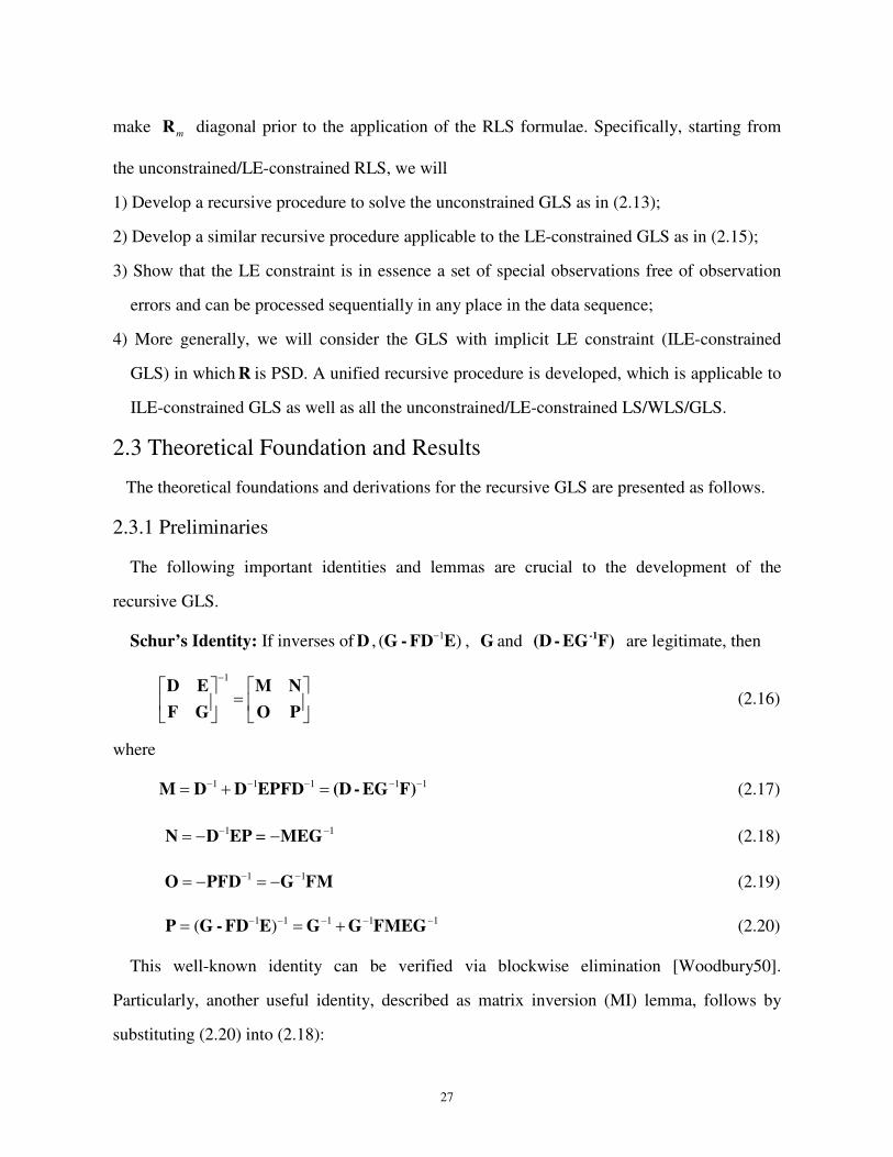
Schur’s Identity: If inverses of D , 1( )−G - FD E , G and -1(D - EG F) are legitimate, then
1−
=
D E M N
F G O P (2.16)
where
1 1 1 1 1− − − − −= + =M D D EPFD (D - EG F) (2.17)
1 1=
− −= − −N D EP MEG (2.18)
1 1− −= − = −O PFD G FM (2.19)
1 1 1 1 1( )− − − − −= = +P G - FD E G G FMEG (2.20)
This well-known identity can be verified via blockwise elimination [Woodbury50].
Particularly, another useful identity, described as matrix inversion (MI) lemma, follows by
substituting (2.20) into (2.18):

28
MI Lemma: If inverses of matrices D , G and 1( )−G - FD E exist, then
1 1 1( )− − −= +-1 -1 -1 -1(D - EG F) D D E G - FD E FD (2.21)
The MI lemma has the following important corollary which is the basis of the conventional
RLS:
Corollary of MI Lemma: If inverses of matrices D ,G and 1( )T −+G E D E exist, then
1 1 1 1 1 1 1( )T T T− − − − − − −+ = − +(D E G E) D D E ED E G ED (2.22)
Actually, this corollary contains such a bidirectional causal relation as: Given 1−D and 1−G ,
the existence of 1 1( )T − −G - E D E is equivalent to the existence of 1 1T − −+(D E G E) , which is an
important basis for Facts 1 and 2 regarding the conventional unconstrained and LE-constrained
RLS solutions, respectively (see the Introduction).
2.3.2 Recursive solutions to unconstrained GLS
First, the recursive solution to the unconstrained GLS is investigated, which is identical to
the following batch one:
Fact 3 (Batch solution to unconstrained GLS): Iff rank( ) N=H , the normal equation
(2.13) has a unique solution:
1( )
ˆ
T
T
− =
=
C H WH
x CH Wz (2.23)
In general, iff rank( )m
N=H , the GLS problem with data up to m has a unique solution:
1( )
ˆ
T
m m m m
T
m m m m m
− =
=
C H W H
x C H W z (2.24)
The batch solutions, as in (2.23) and (2.24), can be computed in the same recursive way as
the conventional RLS as long as the following decorrelation is applied.
Definition 1 (Last-row-column (LRC) decorrelation): Given PDm
R (2.12), the following
pair of nonsingular matricesm
Q and T
mQ can diagonalize the last row and column of
mR :

29
T
m m m m′ =R Q R Q
1diag{ , }T
m m m mr D R−= −R (2.25)
with( 1) ( 1)
1
m m m
m T
D− × − − =
IQ
0 and 1
1m m mD R
−−= R (2.26)
Equation (2.25) can be easily verified. In addition, using a series of successive LRC
decorrelations, m
R can be transformed into a diagonal matrix, as in Proposition 1.
Proposition 1 (Inverse decomposition of a PD matrix): Given PD m
R (2.12), the
following equality holds for 1 m M< ≤ :
1: 1: 1 2diag{ , , , }T
m m m mr r r′ ′=Q R Q L (2.27)
with
2
1:
1
0 1
0 0 1
m
m
D D− − =
Q
L
M O O
L
(2.28a)
T
m m m mr r D R′ = − (2.28b)
and 1
1m m mD R
−−= R (2.28c)
A proof of this proposition is given in Appendix A. Note that, althoughm
R is transformed
into a diagonal matrix, the transformation in (2.27) is conceptually different from the
conventional matrix diagonalization where the pairwise transformation matrices are mutual
inverses. In fact, the one in (2.27) is in essence an inverse process of the symmetric indefinite
factorization which is an alternative form of the Cholesky decomposition (factorization)
[Watkins91] [Ogita12]. In previous work as in [Petkovic09] [Karlsson06], this inverse
transformation is usually treated as a two-stage procedure of decomposition and inversion
[Ogita10]. Proposition 1 provides a method to obtain the inverse decomposition directly.
Actually, as shown in (2.25), the transformation in (2.27) is not only a mathematical inversion

30
process of the Cholesky decomposition. It has specific interpretations of error-correlation
deduction in practical applications where R is set as observation error covariance (see Chapter
4). In particular, it is clear that 1:mQ in (2.28a) can be computed recursively as
1
1:( 1) 1:( 1) 1
1:0 1 0 1
m m m m m
m
D R−
− − −− − = =
Q Q RQ (2.28d)
which is similar to the recursive (inverse) Cholesky decomposition [Gustavson00] [Bjarne01]
[Bjarne02]. In fact, the recursive computation in (2.28d) can be further simplified. Applying
this recursive transformation as well as the RLS formulae to the unconstrained GLS, the
recursive solution can thus be developed as follows.
Theorem 1 (Recursive GLS): If0
rank( )M
N=H and 0M M< , the unconstrained GLS
problem (2.10) has the following recursive solution:
1 1
1
ˆ ˆ ˆ( )m m m m m m
T
m m m m m
z H− −
−
′ ′= + −
= −
x x K x
C C K S K (2.29)
for 0M m M< ≤ with
1
1
1
T
m m m m m
T
m m m m
H H r
H
−
−−
′ ′ ′ +
′
S C
K C S
≜
≜ (2.30)
1
1
T
m m m m
T
m m m m
T
m m m m
H H D
r r D R
z z D
−
−
′ ′ ′ −′ ′ ′−
′ ′ ′−
H
z
�
�
�
(2.31a)
1:( 1)
1
T
m m m
m m m
R R
D R
−
−
′ =
′ ′
Q
Di� (2.31b)
1:( 1) 1:( 1)
1:1
m m m
m T
D− − ′− =
Q QQ
0 (2.32a)
1
1
1
1
[ ]
diag( , )
[ ]
T T T
m m m
m m m
T T T
m m m
H
r
z
−
−−
−
′ ′ ′ =
′= ′ ′ ′=
H H
Di Di
z z
(2.32b)
and
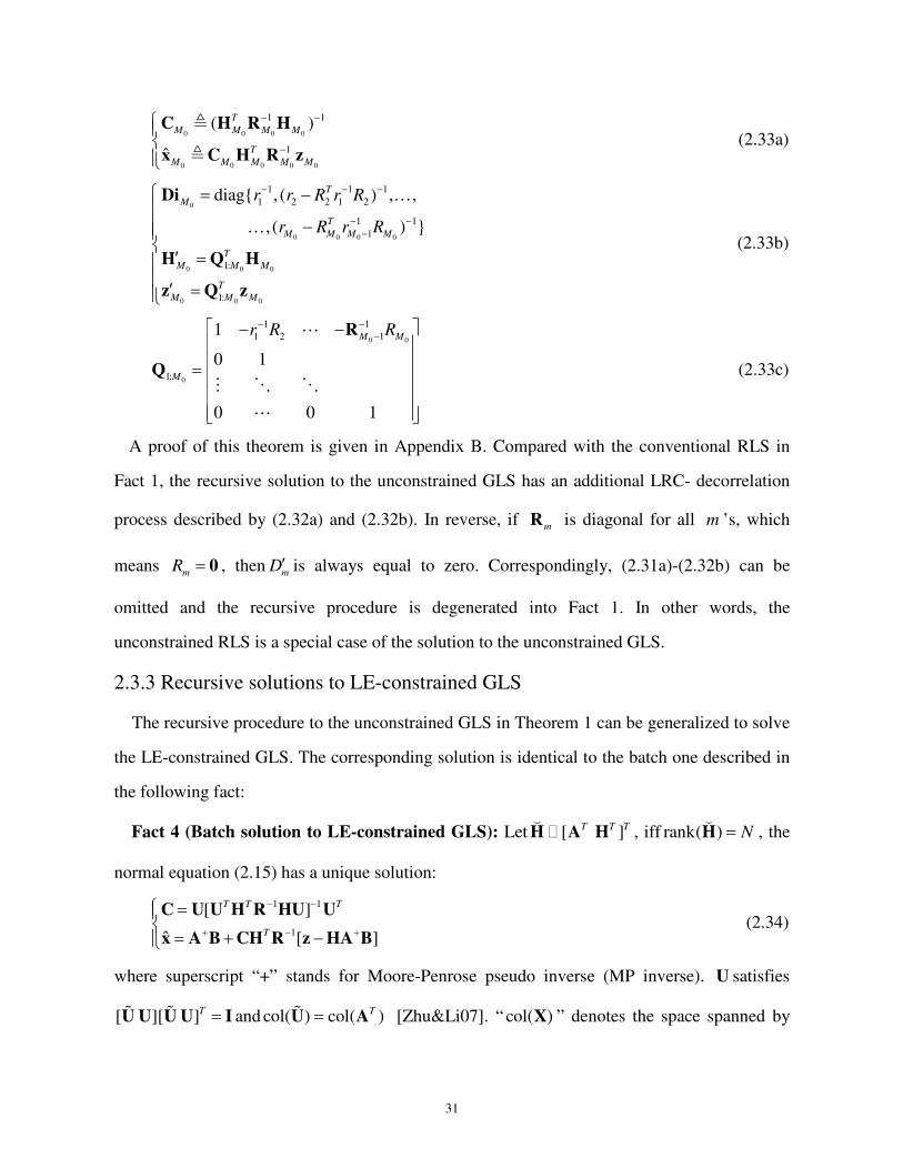
31
0 0 0 0
0 0 0 0 0
1 1
1
( )
ˆ
T
M M M M
T
M M M M M
− −
−
C H R H
x C H R z
≜
≜ (2.33a)
0
0 0 0 0
0 0 0
0 0 0
1 1 1
1 2 2 1 2
1 1
1
1:
1:
diag{ , ( ) , ,
, ( ) }
T
M
T
M M M M
T
M M M
T
M M M
r r R r R
r R r R
− − −
− −−
= −
−
′ = ′ =
Di
H Q H
z Q z
K
K (2.33b)
0 0
0
1 1
1 2 1
1:
1
0 1
0 0 1
M M
M
r R R− −− − −
=
R
Q
L
M O O
L
(2.33c)
A proof of this theorem is given in Appendix B. Compared with the conventional RLS in
Fact 1, the recursive solution to the unconstrained GLS has an additional LRC- decorrelation
process described by (2.32a) and (2.32b). In reverse, if m
R is diagonal for all m ’s, which
means m
R = 0 , thenm
D′ is always equal to zero. Correspondingly, (2.31a)-(2.32b) can be
omitted and the recursive procedure is degenerated into Fact 1. In other words, the
unconstrained RLS is a special case of the solution to the unconstrained GLS.
2.3.3 Recursive solutions to LE-constrained GLS
The recursive procedure to the unconstrained GLS in Theorem 1 can be generalized to solve
the LE-constrained GLS. The corresponding solution is identical to the batch one described in
the following fact:
Fact 4 (Batch solution to LE-constrained GLS): Let [ ]T T TH A H(� , iff rank( ) N=H
(, the
normal equation (2.15) has a unique solution:
1 1
1
[ ]
ˆ [ ]
T T T
T
− −
+ − +
=
= + −
C U U H R HU U
x A B CH R z HA B (2.34)
where superscript “+” stands for Moore-Penrose pseudo inverse (MP inverse). U satisfies
[ ][ ]T =U U U U I% % and col( ) col( )T=U A% [Zhu&Li07]. “ col( )X ” denotes the space spanned by
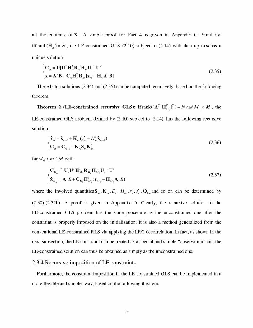
32
all the columns of X . A simple proof for Fact 4 is given in Appendix C. Similarly,
iff rank( )m
N=H(
, the LE-constrained GLS (2.10) subject to (2.14) with data up to m has a
unique solution
1 1
1
[ ]
ˆ [ ]
T T T
m m m m
T
m m m m m
− −
+ − +
=
= + −
C U U H R H U U
x A B C H R z H A B (2.35)
These batch solutions (2.34) and (2.35) can be computed recursively, based on the following
theorem.
Theorem 2 (LE-constrained recursive GLS): If0
rank([ ] )T T T
M N=A H and 0M M< , the
LE-constrained GLS problem defined by (2.10) subject to (2.14), has the following recursive
solution:
1 1
1
ˆ ˆ ˆ( )m m m m m m
T
m m m m m
z H− −
−
′ ′= + −
= −
x x K x
C C K S K (2.36)
for 0M m M< ≤ with
0 0 0 0
0 0 0 0 0
1 1[ ]
ˆ ( )
T T T
M M M M
T
M M M M MB B
− −
+ +
= + −
C U U H R H U U
x A C H z H A
≜ (2.37)
where the involved quantitiesm
S ,m
K ,m
D ,m
H ′ ,m
r′ ,m
z′ , 1:mQ and so on can be determined by
(2.30)-(2.32b). A proof is given in Appendix D. Clearly, the recursive solution to the
LE-constrained GLS problem has the same procedure as the unconstrained one after the
constraint is properly imposed on the initialization. It is also a method generalized from the
conventional LE-constrained RLS via applying the LRC decorrelation. In fact, as shown in the
next subsection, the LE constraint can be treated as a special and simple “observation” and the
LE-constrained solution can thus be obtained as simply as the unconstrained one.
2.3.4 Recursive imposition of LE constraints
Furthermore, the constraint imposition in the LE-constrained GLS can be implemented in a
more flexible and simpler way, based on the following theorem.
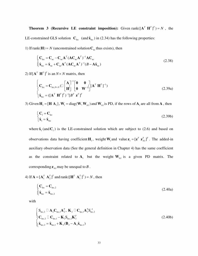
33
Theorem 3 (Recursive LE constraint imposition): Given rank([ ] )T T T N=A H , the
LE-constrained GLS solution lecC (and lecx ) in (2.34) has the following properties:
1) If rank( ) N=H (unconstrained solution ucC thus exists), then
1
lec uc uc uc uc
1
lec uc uc uc uc
( )
ˆ ˆ ˆ( ) ( )
T T
T TB
−
−
= −
= + −
C C C A AC A AC
x x C A AC A Ax (2.38)
2) If[ ]T T TA H is an N N× matrix, then
1
1
lec lec, 1
1
lec
( [ ] )
ˆ ([ ] ) [ ]
T T
N N
T T T T T TB
−
−× −
−
=
=
A 0 0C C A H
H 0 W
x A H z
� (2.39a)
3) Given 1 1[ ]=H H A , 1 A1diag( , )=W W W and A1W is PD, if the rows of 1A are all from A , then
1 lec
1 lecˆ ˆ
=
=
C C
x x (2.39b)
where 1x (and 1C ) is the LE-constrained solution which are subject to (2.6) and based on
observations data having coefficient 1H , weight 1W and value 1 A1[ ]T T T=z z z . The added-in
auxiliary observation data (See the general definition in Chapter 4) has the same coefficient
as the constraint related to 1A but the weight A1W is a given PD matrix. The
corresponding A1z may be unequal to B .
4) If 1 2[ ]T T T=A A A and 1rank([ ] )T T TN=H A , then
lec lec,2
lec lec,2ˆ ˆ
=
=
C C
x x (2.40a)
with
1
lec,2 2 lec,1 2 2 lec,1 2 lec,2
lec,2 lec,1 2 lec,2 2
lec,2 lec,1 2 2 2 lec,1
S , S
S
ˆ ˆ ˆ( )
T T
T
−
− = + −
A C A K C A
C C K K
x x K B A x
� �
� (2.40b)

34
and
1 1
lec,1 1 1 1 1
lec,1 1 1 lec,1 1 1
( )
ˆ ( )
T T T
TB B
− −
+ +
=
= + −
C U U H R HU U
x A C H z HA (2.40c)
where 1 1 1 1[ ][ ]T =U U U U I% % and 1 1col( ) col( )T=U A% .
A proof of Theorem 3 is in Appendix E. In this theorem, Statement 1) provides a formula to
compute the LE-constrained solution from the corresponding unconstrained solution (if the
latter exists). Statement 2) presents the specific solution which is exactly determined by the
observation and constraint. Statement 3) shows that those observations which have the same
coefficient as the constraint have no effect on the solution. Statement 4) indicates that multiple
LE constraints can be imposed sequentially.
In addition, ucC in Statement 1) and lec,1C Statement 4) can both be viewed as special
initializations for the recursive GLS, within which no constraint or only a part of constraints,
accompanied by a part of observations, are processed. In Statement 4), the constraints related
to 2A can be inserted into any place in the remaining-observation sequence. It is because: the
observations prior to the constraint 2A plus the existing initialization form a new augmented
initialization with partial constraints; according to statement 4), after being processed,
the 2A constraints and the previous observations & constraints compose another new
initialization. Correspondingly, the fact that the overall procedure leads to the exact GLS
solution can be shown by Theorem 2.
In summary, combining Theorems 2 and 3, it can be concluded that the LE constraints can
be wholly or partially imposed onto the initialization, and they can also be processed posterior
to the initialization if the corresponding unconstrained solution exists. After the initialization,
the remaining constraints can be processed sequentially at any place in the to-be-processed
observation sequence. In other words, an LE constraint plays a role of a special observation
free of error: 0A
r = , and the crossing terms between the constraint and other
35
observations/constraintsA
R = 0 . When the constraint is processed in the recursive GLS,
lec -1 -1 -10
limT T T
rr
→′ ′= = = +S AC A A C A AC A I (2.41)
where 1−C is the unconstrained/LE-constrained covariance-like matrix prior to the current
constraint imposition.
2.3.5 Recursive solution to GLS with Implicit LE constraint
According to the above observation-constraint unification, the unified observations in the
LE-constrained GLS problem defined by (2.10) subject to (2.14) has [ ]T T T=H H A(
and
[ ]T T T=z z B(
, and the corresponding unified weight is
1diag{ ,[ ]}−= +∞ +∞W R(
L (2.42a)
One major challenge using W(
is that “ +∞ ” may not be exactly expressed in practical
applications. Alternatively, if we start from the OEC-like matrix
diag{ , }=R R 0(
(2.42b)
then the unified form of the LE-constrained GLS, as well as the solution, can take advantage of
the recursive-constraint-imposition formula (2.41) and can thus avoid the possible numerical
problem caused by infinite weights.
More generally, starting from a PSD OEC-like matrix, the unified form of the
LE-constrained GLS can be extended to resolve some application problems where the LE
constraint is embedded in the data sequence implicitly. Correspondingly, an equivalent explicit
GLS formulation and the (recursive) solutions are exploited. This combination of GLS
formulation and solution is in essence a GLS problem with a set of implicit LE constraints.
The recursive solution to the GLS with implicit LE constraint (ILE-constrained GLS) is
investigated, which is based on the following decorrelation techniques.
Proposition 2 (LRC decorrelation of a special PSD matrix): Consider the following
special matrix
36
1 2
2
2 2
a a
a T
a a
R
R r
+ ++
+ +
=
RR (Note: not as generic as 1m a= +R ) (2.43a)
with, 1
1
, 1 1, 1
a a a
a T
a a a a
++
+ + +
=
R RR
R Rand 2 2 1, 2
TT T
a a a aR R R+ + + +′′ = , where 2a
r + is a scalar, 1, 1a a+ +R is a
scalar/square matrix, and vector 2aR +′′ occupies the same rows as
aR . If 1a+R is PSD,
aR is PD,
and 1rank( ) rank( )a a+ =R R , then
1
2 2 2 1 2 2 2diag( , )T T
a a a a a a a ar R R
−+ + + + + + +′′ ′′= −Q R Q R R
( ( (2.43b)
with
1
2
1
2
1
a a
a
a
T
R−
++
+
′′ − =
RI
Q 0
0
(.
This proposition discloses that the last row and column of the PSD matrix 2a+R defined in
(2.43a) can be diagonalized usinga
R , the leading maximum-rank PD principal minor of 1a+R ,
and the corresponding cross subvector 2aR +′′ only. A proof is given in Appendix F.
Furthermore, from [Meyer00], for an arbitrary PSDm
R as in (2.12), there exists a pair of
permutation matrices T
mQ% and
mQ% with which the orders of the rows and columns of 1m−R can
be symmetrically adjusted such that
1T m m
m m m mT
m m
R
R r
− = =
RQ R Q R
% %% % %
% with
1
1
*
* *
m
m
−−
′′ =
RR% ,
and 1 1rank( ) rank( )m m− −′′ =R R , where
*
m
m
RR
′′ =
% andm
R′′ comes from the same rows (of 1m−R ) as
1m−′′R . In other words, 1m−′′R is a maximum-rank PD principal minor of 1m−R and is promoted
forwards as in 1m−R% (with accordance to Proposition 2). All the not-shown terms are marked
by “* ”. Applying Proposition 2 tom
R% , we have
1diag( , )T T
m m m m m m mr−′ ′ ′=Q Q R Q Q R
( (% % % (2.44)
37
with 1
1
m m
m T
D− −′ =
IQ
0
%(,
1
1m m
m
RD
−−′′ ′′ −
=
R
0% (2.45a)
and 1
1
T
m m m m mr r R R
−−′ ′′ ′′ ′′= − R (2.45b)
Note that the permutation-matrix pair of T
mQ% and
mQ% only adjusts the orders of
mR ’s rows and
columns and thus turnsm
R and 1m−R intom
R% and 1m−R% , respectively. The other pair of T
m′Q
( and
m′Q
( has no effect on the orders of
mR% ’s rows and columns. Therefore, the reverse pair of
mQ%
and T
mQ% can recover the original orders of the adjusted rows and columns of
mR . Obviously,
the adjustment also turns 1m−R% into 1m−R . That is,
1diag( , )T T T
m m m m m m m m mr−′ ′ ′=Q Q Q R Q Q Q R
( (% % % % (2.46a)
Namely,
1diag( , )T
m m m m mr− ′=Q R Q R
( ( (2.46b)
with 1
1
T m m
m m m m T
D− −
′= =
IQ Q Q Q
0
(( (
% % . (2.47a)
Here, the thm row of m
Q% has always a form as[ 1]T0 , so it can be easily verified that
1
1
11
m m
m
m
RD
−−′′ ′′ −
− =
R
Q 0
(
% (2.47b)
In other words, m
D(
is adjusted fromm
D% in such a way: keeping the orders of 1
1m mR
−−′′ ′′−R ’s entries
and inserting these zeros in the “0” of m
D% to those rows which are not occupied by 1m−′′R .
Actually, these zero rows have no effect on the LRC decorrelation. That is,
1
1
T T
m m m m m m m mr r D R r R R
−−′ ′′ ′′ ′′= − = − R
( (2.48a)
Similarly,
1
1 1 1
1
1 1 1
T T
m m m m m m m m
T T
m m m m m m m m
H H D H R
z z D z R
−− − −
−− − −
′ ′′ ′′ ′′− = −′ ′′ ′′ ′′− = −
H R H
z R z
(�
(�
(2.48b)
38
where 1m−′′H occupies the rows of 1m−H which have the same (row) numbers as those of 1m−′′R in
1m−R , so is 1m−′′z . In brief, the last row and column of a PSD matrixm
R can always be
diagonalized using a pair of T
mQ(
andm
Q(
. m
D(
inm
Q(
, as well asm
D% , depends only on 1m−′′R (a
maximum-rank PD principal minor of 1m−R ) and the corresponding cross subvectorm
R′′ . To
determine 1m−′′R , the following proposition can be utilized.
Proposition 3 (Determination of maximum-rank PD principal minor): Consider the
following PSD (or PD) matrix
1
1
1 1
a a
a T
a a
R
R r
++
+ +
=
RR
Suppose that a′′R is a maximum-rank PD minor of
aR . Correspondingly, 1a
R + ’s subvector
1aR +′′ occupies the same rows as
a′′R does. If 1
1 1 1 1( ) 0T
a a a a ar r R R
−+ + + +′ ′′ ′′ ′′− ≠R� , then
1
1
1 1
a a
a T
a a
R
R r
++
+ +
′′ ′′ ′′ = ′′
RR is a maximum-rank PD minor of 1a+R ; otherwise, if 1 0
ar +′ = , then
a′′R is a
maximum-rank PD principal minor of 1a+R .
A proof of Proposition 3 is given in Appendix G. Using Proposition 3, a maximum-rank PD
principal minor of each m
R can be determined recursively. The implementation of
Proposition 3 is presented in Procedure 1 in Sec. 2.4. Based on Propositions 2 and 3, we define
the generalized LRC decorrelation as follows.
Definition 2 (Generalized LRC decorrelation): Given a PSD m
R as in (2.12), the pair of
T
mQ(
and m
Q(
defined by (2.47a) can perform a decorrelation over the last row and column (as
in (2.46b)).
Clearly, after applying a set of successive generalized LRC decorrelations tom
R , we can
draw a conclusion similar to Proposition 1 as follows.
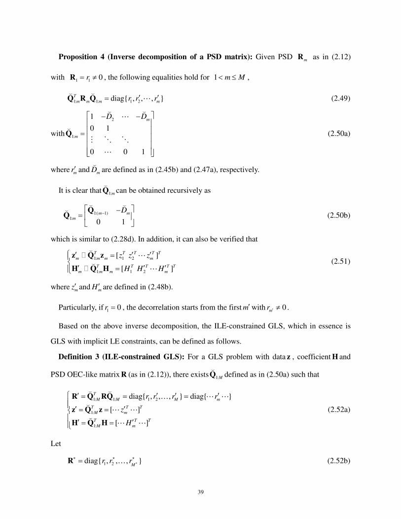
39
Proposition 4 (Inverse decomposition of a PSD matrix): Given PSD m
R as in (2.12)
with 1 1 0r= ≠R , the following equalities hold for 1 m M< ≤ ,
1: 1: 1 2diag{ , , , }T
m m m mr r r′ ′=Q R Q
( (L (2.49)
with
2
1:
1
0 1
0 0 1
m
m
D D − − =
Q
( (L
(
M O O
L
(2.50a)
wherem
r′ andm
D(
are defined as in (2.45b) and (2.47a), respectively.
It is clear that 1:mQ(
can be obtained recursively as
1:( 1)1:
0 1
m m
m
D− −
=
( ((
(2.50b)
which is similar to (2.28d). In addition, it can also be verified that
1: 1 2
1: 1 2
[ ]
[ ]
T T T T T
m m m m
T T T T T
m m m m
z z z
H H H
′ ′ ′=
′ ′ ′=
z Q z
H Q H
(� L
(� L
(2.51)
wherem
z′ andm
H ′ are defined in (2.48b).
Particularly, if 1 0r = , the decorrelation starts from the first m′with 0m
r ′ ≠ .
Based on the above inverse decomposition, the ILE-constrained GLS, which in essence is
GLS with implicit LE constraints, can be defined as follows.
Definition 3 (ILE-constrained GLS): For a GLS problem with data z , coefficient H and
PSD OEC-like matrix R (as in (2.12)), there exists 1:MQ(
defined as in (2.50a) such that
1: 1: 1 2
1:
1:
diag{ , , , } diag{ }
[ ]
[ ]
T
M M M m
T T T
M m
T T T
M m
r r r r
z
H
′ ′ ′ ′= = = ′ ′= = ′ ′= =
R Q RQ
z Q z
H Q H
( (K L L
(L L
(L L
(2.52a)
Let
1 2diag{ , , , }M
r r r ∗∗ ∗ ∗=R K (2.52b)
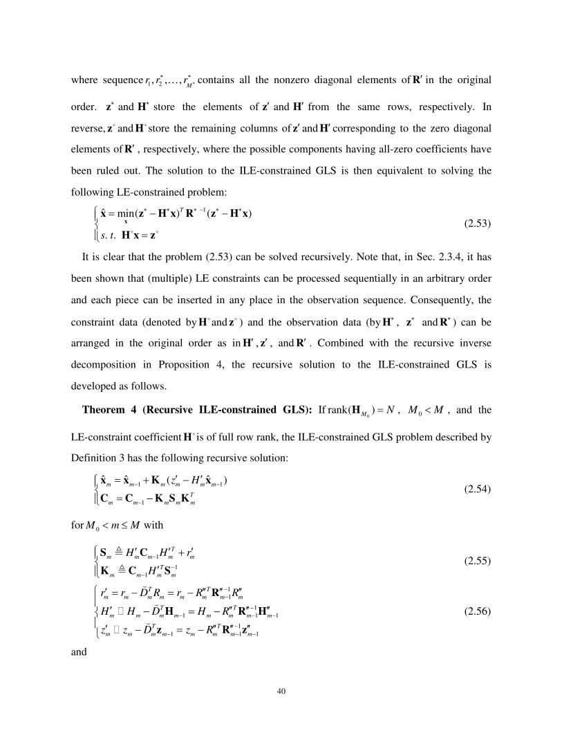
40
where sequence 1 2, , ,M
r r r ∗∗ ∗K contains all the nonzero diagonal elements of ′R in the original
order. ∗z and ∗H store the elements of ′z and ′H from the same rows, respectively. In
reverse, zo and Ho store the remaining columns of ′z and ′H corresponding to the zero diagonal
elements of ′R , respectively, where the possible components having all-zero coefficients have
been ruled out. The solution to the ILE-constrained GLS is then equivalent to solving the
following LE-constrained problem:
1ˆ min( ) ( )
. .
T
s t
∗ ∗ ∗ − ∗ ∗ = − −
=
xx z H x R z H x
H x zo o
(2.53)
It is clear that the problem (2.53) can be solved recursively. Note that, in Sec. 2.3.4, it has
been shown that (multiple) LE constraints can be processed sequentially in an arbitrary order
and each piece can be inserted in any place in the observation sequence. Consequently, the
constraint data (denoted by Hoand zo ) and the observation data (by ∗H , ∗z and ∗R ) can be
arranged in the original order as in ′H , ′z , and ′R . Combined with the recursive inverse
decomposition in Proposition 4, the recursive solution to the ILE-constrained GLS is
developed as follows.
Theorem 4 (Recursive ILE-constrained GLS): If0
rank( )M
N=H , 0M M< , and the
LE-constraint coefficient Ho is of full row rank, the ILE-constrained GLS problem described by
Definition 3 has the following recursive solution:
1 1
1
ˆ ˆ ˆ( )m m m m m m
T
m m m m m
z H− −
−
′ ′= + −
= −
x x K x
C C K S K (2.54)
for 0M m M< ≤ with
1
1
1
T
m m m m m
T
m m m m
H H r
H
−
−−
′ ′ ′ +
′
S C
K C S
≜
≜ (2.55)
1
1
1
1 1 1
1
1 1 1
T T
m m m m m m m m
T T
m m m m m m m m
T T
m m m m m m m m
r r D R r R R
H H D H R
z z D z R
−−
−− − −
−− − −
′ ′′ ′′ ′′= − = −
′ ′′ ′′ ′′− = − ′ ′′ ′′ ′′− = −
R
H R H
z R z
(
(�
(�
(2.56)
and
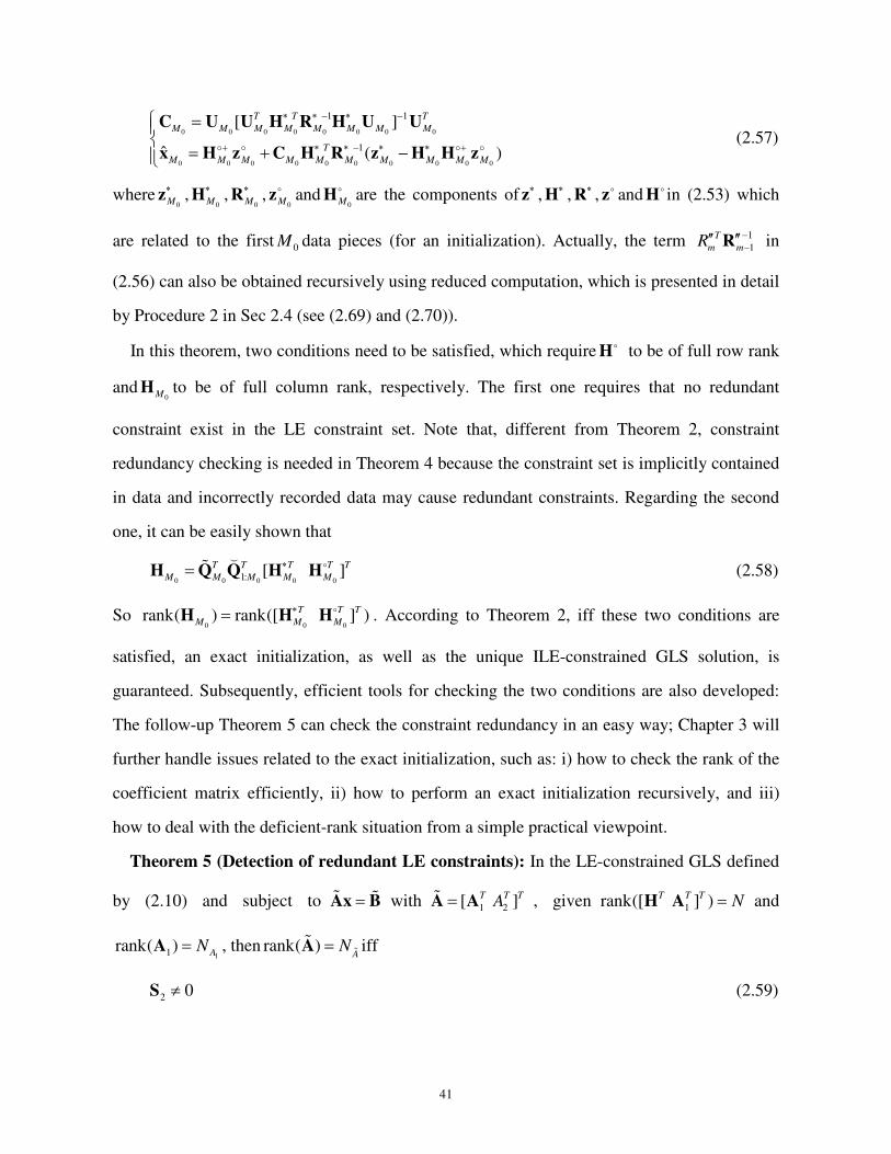
41
0 0 0 0 0 0 0 0
0 0 0 0 0 0 0 0 0 0
1 1
1
[ ]
ˆ ( )
T T T
M M M M M M M M
T
M M M M M M M M M M
∗ ∗ − ∗ −
+ ∗ ∗ − ∗ ∗ +
=
= + −
C U U H R H U U
x H z C H R z H H z� � � � (2.57)
where0M
∗z ,0M
∗H ,0M
∗R ,0Mzo and
0MHo are the components of ∗z , ∗H , ∗R , zo and Ho in (2.53) which
are related to the first 0M data pieces (for an initialization). Actually, the term 1
1
T
m mR
−−′′ ′′R in
(2.56) can also be obtained recursively using reduced computation, which is presented in detail
by Procedure 2 in Sec 2.4 (see (2.69) and (2.70)).
In this theorem, two conditions need to be satisfied, which require Ho to be of full row rank
and0M
H to be of full column rank, respectively. The first one requires that no redundant
constraint exist in the LE constraint set. Note that, different from Theorem 2, constraint
redundancy checking is needed in Theorem 4 because the constraint set is implicitly contained
in data and incorrectly recorded data may cause redundant constraints. Regarding the second
one, it can be easily shown that
0 0 0 0 01: [ ]T T T T T
M M M M M
∗=H Q Q H Ho(
% (2.58)
So 0 0 0
rank( ) rank([ ] )T T T
M M M
∗=H H Ho . According to Theorem 2, iff these two conditions are
satisfied, an exact initialization, as well as the unique ILE-constrained GLS solution, is
guaranteed. Subsequently, efficient tools for checking the two conditions are also developed:
The follow-up Theorem 5 can check the constraint redundancy in an easy way; Chapter 3 will
further handle issues related to the exact initialization, such as: i) how to check the rank of the
coefficient matrix efficiently, ii) how to perform an exact initialization recursively, and iii)
how to deal with the deficient-rank situation from a simple practical viewpoint.
Theorem 5 (Detection of redundant LE constraints): In the LE-constrained GLS defined
by (2.10) and subject to =Ax B% % with 1 2[ ]T T TA=A A% , given 1rank([ ] )T T T
N=H A and
11rank( )A
N=A , then rank( )A
N=A %% iff
2 0≠S (2.59)

42
where 2 2 1 2
TA AS C� , 1 1
1 1 1 1 1 1 1 1[ ( ) ]T T T− −=C U U H R H U U , and 1U satisfies 1 1 1 1[ ][ ]T =U U U U I% % and
1 1col( ) col( )T=U A% .
A proof of Theorem 5 is given in Appendix H. This theorem indicates that no extra work but
simply calculating m
S can tell whether a piece of new LE constraint is redundant with respect
to the processed ones or not. Once a redundant constraint is detected, a further judgment on
constraint consistency can be made by comparing 2 1ˆA x and 2B . That is, if 2 1 2
ˆA B=x , then the
constraint 2 2A B=x has already been previously “imposed” and can thus be ignored.
Otherwise, if 2 1 2ˆA B≠x , then the constraint is inconsistent with one or more
previously-imposed constraint. Note that, in practical applications, the constraint inconsistency
is mostly caused by incorrectly-recorded data. Therefore, data correctness needs to be
rechecked if an inconsistent LE constraint is found. Finally, it can be verified that the solution
of the LE-constrained GLS is identical to that of the corresponding ILE-constrained GLS with
a PSD OEC-like matrix. Therefore, the latter is a unified and generalized recursive GLS.
2.4 Unified Procedures and Algorithms
During the course of decorrelating the PSD OEC-like matrix, the LRC decorrelation
employs only a maximum-rank PD principal minor of the to-be-decorrelated matrix as well as
the corresponding cross subvector. Therefore, the determination of a maximum-rank PD
principal minor is crucial. This work can be handled by the following recursive procedure
efficiently.
Procedure 1: Determination of maximum-rank PD principal minor
1) 1m = , 1m∗ = ,
D
1 1mmr∗ ′′= = =R R R ( 1 0r ≠ )
R_o 1m=
2) : 1m m= + :

43
Using the row numbers in 1R_om− , pick
mR′′ out of
mR ;
1
1
T
m m m m mr r R R
−−′ ′′ ′′ ′′= − R
2.1) If 0m
r′ = , then
1m m−′′ ′′=R R
2.2) If 0m
r′ ≠ , then : 1m m∗ ∗= + :
D
mmR R∗ ′′= (2.60a)
1D m m
m Tmm m
R
R r∗
−′′ ′′ ′′= = ′′
RR R (2.60b)
R_o [R_o ]m m
m=
3) Repeat 2) till m M= .
Here, m∗ is used to index different recorded maximum-rank PD principal minors. This
indexing method can bring convenience to the follow-up procedure design.
Note that Procedure 1 is mainly for the use of illustrating the determination ofm′′R . In fact,
in the recursive ILE-constrained GLS, it is 1
m
−′′R (or D -1( )m∗R identically) that is directly involved
in the computation. According to Proposition 1, there exists
D D D 1 D
1 2 1 1
D
1:( )
1 ( )
0 1
0 0 1
m m
m
R R∗ ∗
∗
−
− − − − =
R R
Q
L
M O O
L
- 1( )
(2.61)
such that
D -1 D 1 D 1 D 1 D
1 21:( ) 1:( )( ) diag{ , ( ) , , ( ) } T
m m m mr r r∗ ∗ ∗ ∗− − −= ⋅ ⋅R Q QK (2.62)
where it can be easily verified that, for 1 i m∗< ≤ ,
D
i ir r
∗= (2.63)
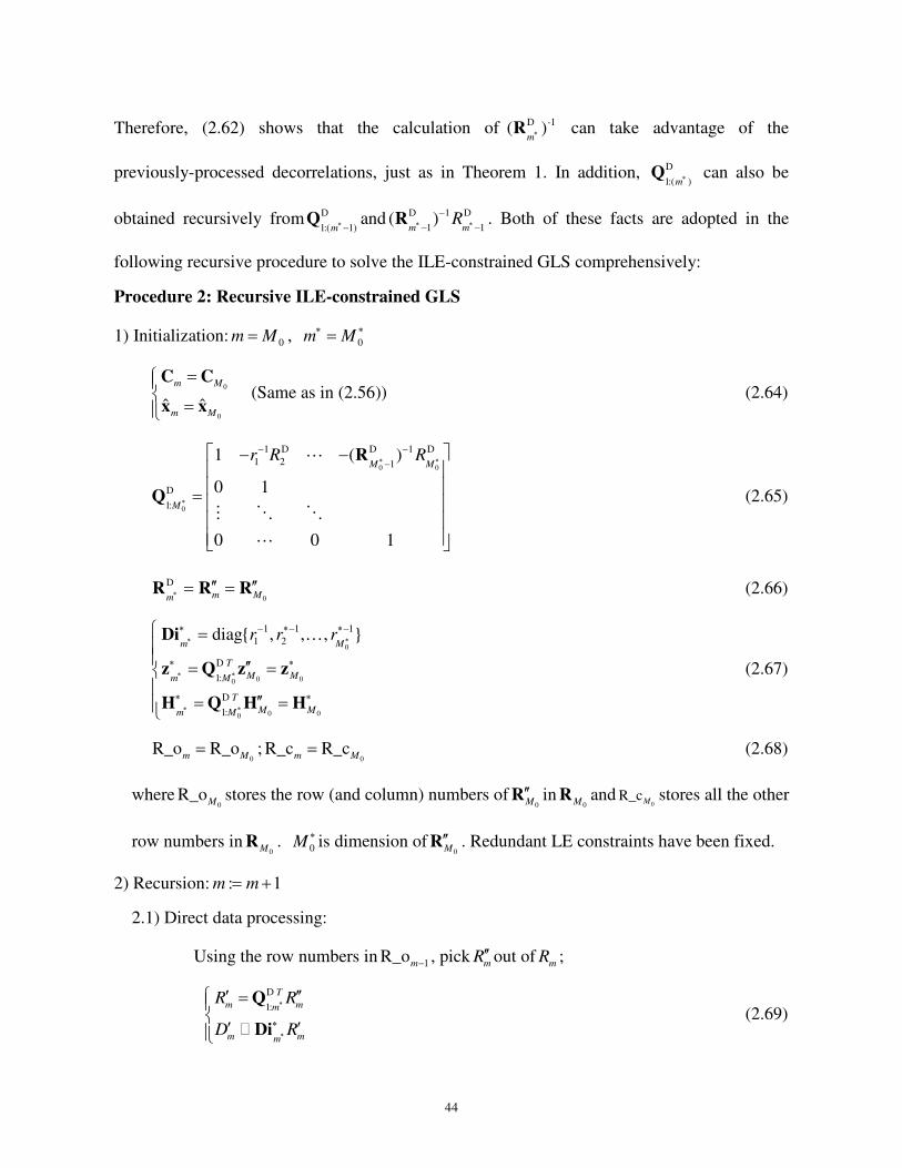
44
Therefore, (2.62) shows that the calculation of D -1( )m∗R can take advantage of the
previously-processed decorrelations, just as in Theorem 1. In addition, D
1:( )m∗Q can also be
obtained recursively from D
1:( 1)m∗−
Q and D 1 D
1 1( )
m mR∗ ∗
−
− −R . Both of these facts are adopted in the
following recursive procedure to solve the ILE-constrained GLS comprehensively:
Procedure 2: Recursive ILE-constrained GLS
1) Initialization: 0m M= , 0m M∗ ∗=
0
0ˆ ˆ
m M
m M
=
=
C C
x x (Same as in (2.56)) (2.64)
0 0
0
1 D D 1 D
1 2 1
D
1:
1 ( )
0 1
0 0 1
M M
M
r R R∗ ∗
∗
− −
− − − =
R
Q
L
M O O
L
(2.65)
0
D
m Mm∗ ′′ ′′= =R R R (2.66)
0
0 00
0 00
1 1 1
1 2
D
1:
D
1:
diag{ , , , }m M
T
M Mm M
T
M Mm M
r r r∗ ∗
∗ ∗
∗ ∗
∗ − ∗− ∗−
∗ ∗
∗ ∗
= ′′= =
′′= =
Di
z Q z z
H Q H H
K
(2.67)
0R_o R_o
m M= ;
0R_c R_c
m M= (2.68)
where0
R_oM
stores the row (and column) numbers of0M
′′R in0M
R and0
R_cM stores all the other
row numbers in0M
R . 0M∗ is dimension of
0M′′R . Redundant LE constraints have been fixed.
2) Recursion: : 1m m= +
2.1) Direct data processing:
Using the row numbers in 1R_om− , pick
mR′′ out of
mR ;
D
1:
T
m mm
m mm
R R
D R
∗
∗∗
′ ′′ =
′ ′
Q
Di� (2.69)
45
T
m m m m
T
m m m m
T
m m m m
r r R D
H H D
z z D
∗
∗
∗
∗
′ ′ ′= − ′ ′= −′ ′= −
H
z
(2.70)
1
1
1
T
m m m m m
T
m m m m
H H r
H
−
−−
′ ′ ′ +
′
S C
K C S
≜
≜ (2.71)
2.1.1) If 0m≠S ,
1 1
1
ˆ ˆ ˆ( )m m m m m m
T
m m m m m
z H− −
−
′ ′= + −
= −
x x K x
C C K S K (2.72)
2.1.2) If 0m=S ( redundant LE constraint),
Fix the constraint set recorded by R_cm
;
2.2) Reserve-data processing:
2.2.1) If 0m
r′ = (constraint),
1R_o R_om m−= ; 1R_c [R_c ]
m mm−= (2.73)
2.2.2) If 0m
r′ ≠ (observation),
1R_o [R_o ]m m
m−= ; 1R_c R_cm m−= (2.74)
: 1m m∗ ∗= + (2.75)
D D
D 1:( 1) 1:( 1)
1:1
mm m
m T
D∗ ∗
∗− −
′ −=
Q QQ
0 (2.76)
1
1
1
1
diag{ , }
[ ]
[ ]
m m m
T T T
m m m
T T T
m m m
r
H
z
∗ ∗ −∗ ∗−
∗ ∗∗ ∗−
∗ ∗∗ ∗−
′ =
′= ′=
Di Di
H H
z z
(2.77)
3) Go to 2) till m M= .
Particularly, in the Initialization described by step 1), the determination of the initial values
0MC and
0ˆ
Mx in (2.64) can be completed by the work in Chapter 3.
46
2.5 Performance Analysis
As a generalized approach, the recursive GLS inherits the recursion-oriented advantages of
the conventional RLS [Zhu&Li07]. It remains a recursive form. The overall computation is
free of direct matrix-inverse operation although matrix inverses are involved in both the
EEC-like matrices and the weight calculations. Particularly, it is also revealed that the LE
constraint can be recursively imposed as a special and even simplified observation set without
resorting to MP-inverse operation. Therefore, the recursive GLS has much more reduced
computational complexity than traditional LE-constrained GLS methods and is thus suitable
for real-time applications. That is, the number of algebraic operations, as well as that of the
required memory locations, is of 2( )O m (order of 2m ) at the thm recursion cycle while the
corresponding batch solutions can cost as high as 2( )O M N . Note that, because of the
increment of nonzero elements contained in each m
R (i.e.,m
R ) amounts to m , the operations
in each cycle may not remain fixed but increase with m . It is because the terms D
1:
T
m mmR R∗′ ′′=Q in
(2.69) and T
m m m mH H D ∗
∗′ ′= − H introduce increasingly more computation during the course of
data accumulation. In particular, the major computation in the step of reserve-data processing
as in 2.2) can be handled in two parallel threads since the formulae (2.70)-(2.72) and the
formulae (2.74)-(2.77) do not rely on each other.
2.6 Appendix
2.6.1 Appendix A
Proof of Proposition 1:
According to (2.25), for 1 m M< ≤ , we have
T
m m m m′=Q R Q R
So 1 1( )T
m m m m
− −′=R Q R Q
1 1
1( ) diag{ , }T
m m m mr
− −− ′= ⋅ ⋅Q R Q

47
1 1
1 11 1
1
( )( ) diag{ , }
1 1
T
T m m
m m m mT Tr
− −− −− −
−
′ ′= ⋅ ⋅
Q 0 Q 0Q R Q
0 0 (2.78)
Further diagonalizing 1m−′R in the similar way, we can get that
1 1
1: 1 2 1:( ) diag{ , , , }T
m m m mr r r
− −′ ′= ⋅ ⋅R Q QL (2.79)
with
1 1
1 12 1
1:1
m
m mT T
− −− −−
Q 0 Q 0Q Q
0 I 0� L
Equivalently,
1 2
1:1
m
m m T T
−
Q 0 Q 0Q Q
0 0 I� L
21
0 1
0 0 1
mD D− − =
L
M O O
L
(2.80)
From (2.79),
1: 1: 1 2diag{ , , , }T
m m m mr r r′ ′=Q R Q L . Done.
2.6.2 Appendix B
Proof of Theorem 1:
According to (2.78),
1 1 1
1diag{ , } T
m m m m mr
− − −− ′= ⋅ ⋅R Q R Q
Then it can be verified that
1T
m m m
−H R H
1 1
1 1 1[ ] diag{ , } [ ]T T T T T T
m m m m m m m mH r H
− −− − −′= ⋅ ⋅H Q R Q H
1 1
1 1 1
T T
m m m m m mH r H
− −− − − ′ ′ ′= +H R H (2.81)

48
with
1
1 1
1
1
1
1 1
T
m m m m m
T
m m m m m
T
m m m m m
H H R
r r R R
z z R
−− −
−−
−− −
′ = −′ = −
′ = −
R H
R
R z
(2.82)
Furthermore, the fact that0
rank( )M
N=H ensures the existence of 1m−C (for 0M m M< ≤ ).
Therefore, similar to the conventional RLS in Fact 1 [Zhu&Li07], we can show from (2.22)
that
1 1( )T
m m m m
− −C H R H�
1 1 1
1 1 1( )T T
m m m m m mH r H
− − −− − − ′ ′ ′= +H R H
1
1 1 ( )T T
m m m m m m m m mH H H r H
−− − ′ ′ ′ ′ ′= − +C C C C
1 1 1
T
m m m m m m m mH− − −′= − = −C K C C K S K (2.83)
and
1ˆ T
m m m m m
−=x C H R z
1 1
1 1 1[ ] diag{ , } [ ]T T T T T T
m m m m m m m m mH r z
− −− − −′= ⋅ ⋅C H Q R Q z
1 1
1 1 1[ ] diag{ , } [ ]T T T T T
m m m m m m mH r z
− −− − −′ ′ ′= ⋅ ⋅C H R z
1 1
1 1 1
T T
m m m m m m m mH r z
− −− − − ′ ′ ′= +C H R z C
According to (2.83),
1 1
1 1 1 1 1 1 1 1( )T T
m m m m m m m m m m mH
− −− − − − − − − −′= −C H R z I K C H R z
1 1ˆ( )
m m m mH− −′= −I K x
1 1 1
1 1 1 1[ ( ) ]T T T T
m m m m m m m m m m m m m m m mH r z H H H r H H r z
− − −− − − −′ ′ ′ ′ ′ ′ ′ ′ ′ ′ ′= − +C C I C C
1 1
1 1 1 1( ) [ ]T T T T
m m m m m m m m m m m m m m mH H H r H H r H H r z
− −− − − −′ ′ ′ ′ ′ ′ ′ ′ ′ ′ ′= + + −C C C C
m mz′= K
As a result, for 0M m M< ≤ ,
49
1 1ˆ ˆ ˆ( )
m m m m m mz H− −′ ′= + −x x K x
Eventually,
1 1 1
1 1
1 1
1
ˆ ( )
ˆ ˆ ( )
( )
T T
M
M M M M M
T T
M M M M M
z H
− − −
− −
− −−
= ′ ′= + − = = −
x H R H H R z
x K x
C H R H C K S K
(2.84)
which is identical to the batch solution (2.23).
Furthermore, according to Proposition 1, for1 m M< ≤ ,
1
1m m mD R
−−= R
1:( 1) 1 1:( 1)
T
m m m mR− − −=Q Di Q
1:( 1) 1 1:( 1)m m m m mR D− − −′ ′= =Q Di Q (2.85)
So in (2.83),
1
1 1
T
m m m m mH H R
−− −′ = − R H 1:( 1) 1 1
T T T
m m m m m m mH D H D− − −′ ′ ′= − = −Q H H
T
m m m mr r D R′ ′ ′= − , and 1
T
m m m mz z D −′ ′ ′= − z
Correspondingly,
1:( 1) 1:( 1) 1:( 1)
1:1 1
m m m m m
m T T
D D− − − ′− − = =
Q Q QQ
0 0
and the formulae at 0m M= come from the definitions.
2.6.3 Appendix C
Proof of Fact 4:
Since R is PD, there exists12
−R such that
1 12 2( )T− −=R R and
1 12 2 1− − −=R R R . Then (2.15) can be
rewritten as
ˆ( )T T T
B
′ ′ ′ ′ =
xH H A H z
λA 0 (2.86)
with12
−′ =H R H and12
−′ =z R z . Applying (1.11) (according to [Zhu&Li07]), iff

50
rank([ ] )T T T N′ =A H , (2.86) as well as (2.15) has a unique solution as
1
1[ ( ) ]
ˆ ( )
MT T T
m mm
T
H H
B B
−
=
+ +
′ ′=
′ ′ ′= + −
∑C U U U U
x A CH z H A (2.87)
Here, (2.87) is identical to (2.34). In addition,
12[ ] diag( , )[ ]T T T T T T−′ =A H I R A H .
Therefore,
rank([ ] ) rank([ ] )T T T T T T′ =A H A H (2.88)
Fact 4 is thus proven.
2.6.4 Appendix D
Proof of Theorem 2:
Since0
rank([ ] )T T T
M N=A H , m
T ( 1 1( )T T
m m m
− −U H R H U� ) exists for 0M m M< ≤ . Similar to
(2.83), we have
1 1 1
1 1 1
T T T
m m m m m m m m mH r H
− − −− − − ′ ′ ′= +H R H H R H
So
1 1[ ]T T T
m m m m
− −=C U U H R H U U
1 1 1
1 1 1[ ]T T T T T
m m m m m mH r H
− − −− − − ′ ′ ′= +U U H R H U U U U (2.89)
Applying (2.22) to the matrix inverse in (2.89), we get
1
1 1 1 1[ ( ) ]T T T T T
m m m m m m m m mH H H r
−− − − −′ ′ ′ ′= − +C U T T U UT U UT U
Note that 1 1
T
m m− −=UT U C . Therefore,
1
1 1 1 1( )T T
m m m m m m m m m mH H H r H
−− − − −′ ′ ′ ′ ′= − +C C C C C
1
T
m m m m−= −C K S K (2.90)
According to (2.35),
1ˆ [ ]T
m m m m m mB B
+ − += + −x A C H R z H A

51
Similar to the proof of Theorem 1, by substitutingm
C with (2.90), we can show that
1 1ˆ ˆ ˆ( )
m m m m m mz H− −′ ′= + −x x K x (2.91)
2.6.5 Appendix E
Proof of Theorem 3:
Statement 1):
This well-known result can be verified from the normal equation (2.15) explicitly. It
discloses that, if rank( ) N=H , lecC can be computed from ucC ( 1 1( )T − −= H R H ) conveniently
via “deducting” a constraint-related term.
Statement 2):
Since[ ]T T TA H is a full-rank square matrix, lecx is an exactly-determined GLS solution:
1
lec 1 2 1 2ˆ ([ ] ) [ ] [ ][ ]T T T T T T T T T−= = +x A H B z T T B z TB T z� (2.93)
According to (2.34), we also have
1 1
lec lec lecˆ ( )T T+ − + −= − +x A C H R HA B C H R z (2.94)
These two lecx ’s are identical for arbitrary z and B , so
1
1 lec
T+ − += −T A C H R HA , 1
2 lec
T −=T C H R
In lec,N N×C defined in (2.39a), replace 1([ ] )T T T −A H with 1 2[ ]T T , then
1
lec, 2 2 lec lec
T T
N N
−× = =C T RT C H R HC (2.95)
Substituting 1 1[ ( ) ]T T T− −U U H R H U U for lecC , we get
1 1
lec, lec[ ( ) ]T T T
N N
− −× = =C U U H R H U U C .
Similarly, lec, lecˆ ˆ
N N× =x x .
Statement 3):
We have
52
1
1 lec 1 1 1 1[ ( ) ]T T T−=A C A U U H W H U U (2.96)
where[ ][ ]T =U U U U I% % and col( ) col( )T=U A% .
Since the rows of 1A are all from A ,
1 =A U 0 , 1 lec =A C 0 . (2.97)
Compute 1C from lecC :
1 1
1 lec lec 1 1 lec 1 1 1 lec( )T T
A
− −= − +C C C A A C A W A C (2.98)
Taking (2.97) in, we get
1 lec=C C (2.99)
Similarly, 1 lecˆ ˆ=x x . End.
Statement 4):
Let12
−′ =H R H and12
−′ =z R z . Then the original LE-constrained GLS is equivalently
transformed to the following LE-constrained LS:
ˆ arg min J=x
x (2.100a)
with ( ) ( )TJ ′ ′ ′ ′= − −z H x z H x (2.100b)
subject to
=Ax B (2.100c)
Correspondingly, we also have
1 1 1
lec,1 1 1 1 1 1 1 1 1
lec,1 1 1 lec,1 1 1 1 1 lec,1 1 1
( ) ( )
ˆ ( ) ( )
T T T T T T
T TB B B B
− − −
+ + + +
′ ′ = =
′ ′ ′= + − = + −
C U U H R HU U U U H H U U
x A C H z HA A C H z H A (2.101)
Then the Statement 2) is equivalent to that
lec lec,2
lec lec,2ˆ ˆ
′ = ′ =
C C
x x (2.102)
A proof of this LS problem will be presented in Chapter 3.

53
2.6.6 Appendix F
Proof of Proposition 2:
Let1
, 1
1
a a a a
a T
−+
+
−=
I R RQ
0 I
(and
1 1
, 1 2
1
a a a a a a
T
T
R− −
+ +′′ − −
=
I R R R
Q 0 I 0
0 0
(.
Clearly, 1a+Q(
, 2a+Q(
andQ(
all have full rank. We have
1
1 1 1 1, 1 , 1 , 1diag( , )T T
a a a a a a a a a a a
−+ + + + + + += −Q R Q R R R R R
( ( (2.103)
Since 1rank( ) rank( )a a+ =R R ,
1
1, 1 1, 1 , 1 , 1
T
a a a a a a a a a
−+ + + + + +′ = − =R R R R R 0 (2.104)
Furthermore,
2 1, 1 1, 2
1
1, 2 2 2 2
a
T T
a a a a a
T T T
a a a a a a
R
R r R R
+ + + + +−
+ + + + +
′ ′= ′ ′′ ′′−
R 0 0
Q R Q 0 R
0 R
( ( (2.105)
with 1
1, 2 1, 2 , 1 2
T
a a a a a a a aR R R−
+ + + + + +′ ′′= −R R and 1, 1 0a a+ +′ =R (from (2.104)). If 1, 2a a
R + +′ ≠ 0 ,
1, 1 1, 2
1
1, 2 2 2 2
rank 2a a a a
T T
a a a a a a
R
R r R R
+ + + +−
+ + + + +
′ ′ ≥ ′ ′′ ′′−
R
R
which implies that 1rank( ) rank( ) 2m m+ ≥ +R R . It is a contradiction. Therefore,
1
1, 2 1, 2 , 1 2
1
1, 2 2 , 1
T
a a a a a a a a
T T T
a a a a a a
R R R
R R
−+ + + + + +
−+ + + +
′ ′′ = − =
′′− =
R R 0
R R 0 (2.106)
Applying (2.106) to 2 2 2
T
a a a+ + +Q R Q( (
, (2.43b) is thus proven.
2.6.7 Appendix G
Proof of Proposition 3:
Since 1 0r ≠ , we have

54
1
1 1
1 1 1 11 1
T
a a a
T T T T
a a a a a a
R
R r R R r
+− −
+ + + +
′′ ′′ ′′ = ′′ ′′ ′ ′′ ′′ ′′
I 0 R 0 I 0 R
R 0 R
It is clear that1
1 1T
a aR−
+
′′ ′′
I 0
Ris a full-rank square matrix.
Therefore, if 1 0a
r +′ ≠ , then 1
a
T
ar +
′′ ′
R 0
0, as well as
1
1
a a
T
a
R
R r
+
+
′′ ′′ ′′
R, is PD. Thus,
1
1
1
a a
a T
a
R
R r
++
+
′′ ′′ ′′ = ′′
RR is a maximum-rank PD principal minor of 1a+R .
If 1 0a
r +′ = , then 1a+R can be diagonalized as diag( , 0)a
R . Thus, 1rank( ) rank( )a a+ =R R .
a′′R is still a maximum-rank PD principal minor of 1a+R .
2.6.8 Appendix H
Proof of Theorem 5:
1 1 1 1[ ][ ]T =U U U U I% % and 1 1col( ) col( )T=U A% imply that, for an arbitrary row vectora
A ,
1
T
aA =U 0 ⇔ 1col( )T T
aA ∈ A . (2.107)
First, if A% has full row rank, then 2 1col( )T TA ∉ A . According to (2.107), we have 2 1
TA ≠U 0 .
As a result,
1 1
2 2 1 1 1 1 2( ) 0T T T TA A
− −= ≠S U U H R HU U .
Second, if A% does not have full row rank but 1A does, then 2 1col( )T TA ∈ A . So 2 1
TA =U 0 and
1 1
2 2 1 1 1 1 2( ) 0T T T TA A
− −= =S U U H R HU U
Hence, the theorem is proven.
55
Chapter 3: Completely Recursive Least Squares—Part II:
Recursive Initialization and Deficient-Rank Processing
3.1 Introduction
3.1.1 Background
As reviewed in Chapter 1, a great many methods have been developed to solve the
fundamental and classic problem of linear LS, among which the matrix-inversion-lemma (MI
lemma) based recursive least-squares (RLS) is a milestone. The RLS provides LS solutions in
a sequential way and is thus excellent in computation and storage [Albert65]. It is very suitable
to real-time LS applications and has been widely applied into such areas as signal processing,
control and communication [Goodwin77] [Ljung87] [Chen85] [Haykin01] [Passion98]
[Mikles07].
The RLS was originally applied to solve unconstrained LS problems [Albert65], in which
the equivalency between the recursive and the corresponding batch LS solutions is guaranteed
once the MI-lemma based recursion starts from an exact LS solution on the full-rank initial
data. Recently, reference [Zhou&Li07] discovers that the exact solutions of the linear-equality
(LE) constrained LS problem can be obtained by the same (unconstrained) recursion cycle,
provided that the RLS procedure is appropriately initialized. We aim to make the
unconstrained RLS “complete” in two aspects: in Chapter 2 (Part I), a unified recursive
procedure for all LS, WLS and GLS problems with or without LE constraints is developed,
where an accompanying recursive decorrelation procedure is utilized; in this chapter, we
continue discussing appropriate RLS initialization techniques. As reviewed in Sec. 1.4.2, less
attention has been paid to the RLS initialization in the low-dimensional and high-redundancy
environment. However, for high-dimensional and low-redundancy applications, such as power
system state estimation, it is necessary to develop an efficient exact RLS initialization. In the
existing methods reviewed in Sec. 1.4.2, approximate ones usually are not robust because a
56
better approximation can lead to a poorer numerical condition [Albert65]; it is also not always
realistic to start the recursion with forgoing data having special observation functions for
simple exact initializations [Haykin01] [Hubing91] [Albert65]. Reference [Zhou02] introduces
variants of the Greville formula (order recursion) to develop recursive initializations for RLS.
We will study a simple recursive initialization method for RLS, where only the RLS formulae
are used. In addition, two accessorial issues should also be studied. One is whether and when
the foregoing observations can support an exact and unique RLS initialization, namely
(parameter) observability analysis (or rank check) in engineering. A good practical
observability analysis tool is expected to distinguish theoretical rank deficiency and numerical
rank deficiency (see Sec. 1.4.2). The second issue is how to deal with problems with
insufficient observations. Although the minimum-norm solution, which is the one (among
infinitely many feasible estimates) has the minimum norm and also has a simple analytical
form in batch, is widely adopted in theory [Lawson95] [Zhou02], other choices that may bring
more convenience in practice should also be considered.
Exploiting an efficient and exact initialization for RLS, including the implicit rank check
and deficient-rank processing, is worthwhile and expected to make the RLS more applicable to
large-dimensional applications where exact initializations are costly.
3.1.2 Our Work
This chapter treats the initialization-related issues in the RLS problems, including rank
check, a convenient method to compute the involved matrix inverse/pseudoinverse, and
resolution of underdetermined systems. No extra non-RLS formula but an
auxiliary-observation based procedure is utilized.
The main ideas include: a) introducing a set of simple auxiliary observations to construct a
simple fake RLS initialization; b) developing a series of simple tools to detect and remove
these auxiliary observations as soon as possible (ASAP). More concretely, with our method,
1) The RWLS recursion can start from the first real observation and possible LE constraints
are also imposed recursively;
57
2) The rank of the system is checked implicitly. If the rank is full, the initialization and the
subsequent RLS cycles can be integrated as a whole to yield exact LS solutions;
3) If the rank is deficient, the procedure provides a mapping from the unobservable
(original) estimand to a reduced-dimensional set of alternative variables which are linear
combinations of the original variables and uniquely determined. The consequent estimate is a
set of refined non-redundant observations. The refinement is lossless in the WLS sense: if new
observations are available later, it can take the role of the original data in the recalculation.
4) Furthermore, other simple mapping matrices, which lead to alternative-variable sets
reserving all the uniquely-determined original variables, can also be easily constructed from
the output of the procedure.
With the above settings, our recursive initialization is efficient and the RLS is thus more
applicable to large-scale applications where exact initializations are costly.
In addition, this set of techniques is also applicable to the recursive GLS (RLS) discussed in
Chapter 2 because the proposed initialization is free of the diagonalization process in the GLS.
3.2 Problem Formulation
The purpose is to present a series of initialization techniques to complement the RLS and
solve linear WLS problems with or without LE constraint in a completely recursive manner.
The deficient-rank case in which the estimand can not be uniquely determined by the
observation-and-constraint set is also considered.
3.2.1 WLS and Its Batch Solutions
In a WLS problem
1: 1diag( ) diag([ ])M M
w w= =W w L (3.1a)
Correspondingly,
1: 1
1: 1
[ ]
[ ]
T
M M M
T T T
M M M
z z
H H
= = =
= = =
z z z
H H H
L
L (3.1b)
The objective is to solve

58
ˆ min J=x
x (3.2)
with1( ) ( )
MT T
m m m m mmJ z H w z H
== = − −∑H WH x x (3.3)
where estimand x is a vector containing all the N to-be-determined variables and x the
estimated x . H is observation coefficient (vector) in real-observation function, and z
observation value. Correspondingly, observation coefficient (matrix) H contains all H ’s and
observation-value vector z contains all z ’s. The total number of observation is M and m is
observation (data) index.
First, when there is no constraint, the normal equation is
1 1ˆ( )
M MT T
m m m m m mm mH w H H w z
= ==∑ ∑x (3.4)
which has a unique solution if and only if rank( ) N=H :
1 1
uc 1
1
uc uc 1
( ) ( )
ˆ ( )
MT T
m m mm
MT T T
m m mm
H w H
H w z
− −
=
−
=
= =
= =
∑∑
C H WH
x H WH H Wz C (3.5)
Second, when there is a set of (consistent) LE constraints
B=Ax (3.6)
with constraint coefficient T N×∈A � , constant 1TB ×∈� , and (without loss of generality)
rank( ) T=A , the normal equation is
1 1ˆ( )
M MT T T
m m m m m mm mH w H H w z
B
= =
=
∑ ∑xA
λA 0 (3.7)
which has a unique solution if and only if rank( ) N=H(
:
1
lec
lec lec
[ ]
ˆ [ ]
T T T
TB B
−
+ +
=
= + −
C U U H WHU U
x A C H W z HA (3.8)
where [ ]T T TH A H(� . λ is Lagrange’s multiplier. Superscript “+” stands for the
Moore-Penrose (MP) inverse. U satisfies [ ][ ]T =U U U U I% % and col( ) col( )T=U A% , where
“ col( )X ” denotes the space spanned by all the columns of X .

59
3.2.2 RLS Solutions
The RLS computes the unconstrained WLS solution recursively. That is, the solution in
(3.5) can be calculated by repeating the following recursion cycle (and increasing m% )
sequentially:
0 0 0
0
0 0
1
uc, uc, 1
1
uc, uc, 1 uc,
uc, uc, 1 uc, uc, 1
uc, uc, 1 uc, uc, uc,
ˆ ˆ ˆ( )
T
m m M m m M m M
T
m m m M m
m m m m M m M m
T
m m m m m
H H w
H
z H
−+ − + +
−− +
− + + −
−
+
= + −
= −
S C
K C S
x x K x
C C K S K
ɶ ɶ ɶ ɶ ɶ
ɶ ɶ ɶ ɶ
ɶ ɶ ɶ ɶ ɶ ɶ
ɶ ɶ ɶ ɶ ɶ
≜
≜ (3.9)
where01:rank( )
MN=H and the initial values are
0
0
1
uc,0 1
uc,0 uc,0 1
( )
ˆ
M T
m m mm
M T
m m mm
H w H
H w z
−
=
=
=
=
∑∑
C
x C (3.10)
which are identical to the batch solution with the first 0M data.
Furthermore, reference [Zhu&Li07] shows that the recursion (3.9) is also exact for (3.8),
provided that the constraints are imposed initially:
0
0
1
lec,0 1
lec,0 lec,0 1
[ ( ) ]
ˆ ( )[ ]
MT T T
m m mm
M T
m mm
H w H
B H w B
−
=
+ +
=
=
= + −
∑∑
C U U U U
x A C z HA (3.11)
where01:rank([ ] )T T T
M N=A H .
3.2.3 Our Goals
It is not always easy to find the initial values uc,0C and uc,0x from the forgoing data, and much
less for lec,0C and lec,0x since lec,0C is positive semi-definite (PSD) and thus the MP inverse is
involved. The proposed initialization is to overcome these difficulties. It performs
initializations, imposes LE constraints, and determines the minimal initial data set, in a simple
and totally recursive way. In addition, the rank of the system is checked implicitly. If the rank
is full, an exact initialization is obtained. If the rank is deficient, a practical deficient-rank

60
processing method is proposed to provide a set of refined non-redundant observations.
3.3 Derivations and Developments
The theoretical foundations and derivations for the recursive initialization are still based on
those for the RLS, which include the following preliminaries.
3.3.1 Preliminaries
As reviewed in Sec. 2.3.1, the Schur’s Identity leads to the matrix-inversion (MI) lemma.
The MI lemma has a well-known corollary which is the basis of RLS:
Corollary of MI Lemma: If inverses of matrices D ,G and 1( )T −G - E D E exist, then
1 1 1( )T T T− − −+ = − +-1 -1 -1 -1(D E G E) D D E ED E G ED (3.18)
Particularly, it contains a bidirectional causal relation:
Given 1−D and 1−G , 1 1( )T T− − ⇔ + -1 -1G - E D E (D E G E)
which is an important base to the subsequent development.
3.3.2 Development of Recursive Initialization
In our recursive initialization method, we will first introduce a set of simple auxiliary
observations to construct a fake initialization which allows the RLS recursion to start from the
piece of observation data. Then during the course of real observation data processing, we
delete these auxiliary observations ASAP using the corresponding canceling observations.
Therefore, to present the recursive initialization, three types of unconventional observations
are introduced first:
Simple auxiliary observation (SAO) – a make-up simple observation (direct measurement
of estimand component) utilized for simplicity. Specifically, N different SAO’s are adopted in
this chapter, among which the ths one has the following observation coefficient, data, and
(simple) weight:
au,sH ( 1[0 0 1 0 0 ]s s N
I= � L L ), au,sz , 1
au,s sw p−= (3.19)
where s is SAO index. 0s
p > and the values of au,sz ands
p can be assigned by the user for

61
convenience.
Canceling observation (CO) – a fake observation utilized to counteract the influence of a
specific auxiliary or real observation (RO). Specifically, suppose that the coefficient, value and
weight of the to-be-removed simple observation are H&& , z&&and w&& ( 0> ). Then the corresponding
simple canceling observation (SCO) are H&& , z&& and w− && , respectively.
Pseudo observation (PO) – an “observation” that corresponds to a LE constraint.
Specifically, the tht constraint is a PO havingt
b , t
A and +∞ as data, observation coefficient
and weight, respectively.
Basic Tools
An observation may be removed from the processed observation set using the RLS-based
method conveniently [Albert65]. We introduce the concept of CO and further consider
whether an observation is removable in LE-constrained/unconstrained problems, which leads
to the following tool.
Theorem 1 (Observation removal): In the LE-constrained WLS problem (3.2) with (3.6),
given 1C ( 1( )T T T−U U H WHU U� ) with 1 1 1 2 2 2
T T T= +H WH H W H H W H ,
2C ( 1
1 1 1( )T T T−U U H W H U U� ) exists if and only if 1 1
2 1 2 2( )T − −−H C H W exists. If 2C exists, then
1 1
2 1 1 2 2 1 2 2 2 1( )T T − −= − −C C C H H C H W H C (3.20)
Proof:
In Theorem 1, 1C exits if and only if rank( ) N=H(
(see the derivation for (3.8) in
[Zhu&Li07]). The MI Lemma is applied to expand 2C and the if-and-only-if condition requires
that rank( )H(
remain N after 2 2 2
TH W H is removed.
Theorem 1 has the following corollary:
Corollary 1.1 (Simple observation removal): In the LE-constrained WLS problem (3.2)

62
with (3.6), given 1C ( 1( )T T T−U U H WHU U� ) with 1 1 1 2 2 2
T T TH w H= +H WH H W H ,
2C ( 1
1 1 1( )T T T−U U H W H U U� ) exists if and only if 1
2 1 2 2
TH H w
−≠C holds. If 2C exists, then
1 1
2 1 1 2 2 1 2 2 2 1( )T TH H H w H
− −= − −C C C C C (3.21)
Clearly, this corollary is a simplified case of Theorem 1 and is to remove a single
observation. It indicates that removing a simple observation is equivalent to adding in the
corresponding SCO with the “negative weight”. It is clear that the theorem and corollary is
also applicable to the unconstrained WLS problem. This is the key to the unification of the
unconstrained and LE-constrained RLS.
The Initialization Procedure
Our recursive initialization utilizes the above basic tools to introduce and remove auxiliary
observations. Consequently, an initializing procedure, which is the major focus to be
discussed, is developed to perform a recursive and exact initialization for the LE-constrained
linear LS. The development takes advantage of the following properties of the LE-constrained
WLS solutions:
Theorem 2 (Properties of LE-constrained WLS): Given rank([ ] )T T T N=A H ,
lecC (and lecx ) in (3.8) has the following properties:
1) If rank( ) N=H ( ucC thus exists), then
1
lec uc uc uc uc
1
lec uc uc uc uc
( )
ˆ ˆ ˆ( ) ( )
T T
T TB
−
−
= −
= + −
C C C A AC A AC
x x C A AC A Ax (3.22)
2) If [ ]T T TA H is an N N× matrix, then
1
1
lec lec, 1
1
lec
( [ ] )
ˆ ([ ] ) [ ]
T T
N N
T T T T T TB
−
−× −
−
=
=
A 0 0C C A H
H 0 W
x A H z
� (3.23a)
3) Given 1 1[ ]=H H A , 1 A1diag( , )=W W W , and A1W is PD, if the rows of 1A are all from A ,
63
then
1 lec
1 lecˆ ˆ
=
=
C C
x x (3.23b)
where 1x (and 1C ) is the LE-constrained solution subject to (3.6) and using real observation
data having 1H , 1W and 1 A1[ ]T T T=z z z as the coefficient, weight and value, respectively.
4) If 1 2[ ]T T T=A A A and 1rank([ ] )T T TN=H A , then
lec lec,2
lec lec,2ˆ ˆ
=
=
C C
x x (3.24a)
with
1
lec,2 2 lec,1 2 2 lec,1 2 lec,2
lec,2 lec,1 2 lec,2 2
lec,2 lec,1 2 2 2 lec,1
S , S
S
ˆ ˆ ˆ( )
T T
T
−
− = + −
A C A K C A
C C K K
x x K B A x
� �
� (3.24b)
and
1
lec,1 1 1 1 1
lec,1 1 1 lec,1 1 1
( )
ˆ ( )
T T T
TB B
−
+ +
=
= + −
C U U H WHU U
x A C H W z HA (3.24c)
where 1 1 1 1[ ][ ]T =U U U U I% % and 1 1col( ) col( )T=U A% .
A proof of Theorem 2 is given in Appendix A. In fact, this theorem is a corollary of
Theorem 3 in Part I (Chapter 2), where Statement 1) provides a way to compute lecC from ucC ,
and Statement 2) presents a specific lecC . Statement 3) shows that, if observation coefficient 1H
and constraint coefficient A have common rows 1A , then the observations related to 1A have
no effect on the eventual solution. Statement 4) indicates that multiple constraints can be
imposed recursively (sequentially). Just as Chapter 2 declares, these properties imply that the
LE constraints can be treated as special observations (POs) with +∞ as weights (or
equivalently the observation errors are zero). Each constraint can be processed sequentially in
any place in the overall observation-and-constraint data sequence. Correspondingly,

64
1
lec uc uclim T T
ww
−
→+∞= + =S AC A I AC A (3.25)
In this chapter, for the convenience of description, it is assumed that the LE constraint is
explicitly given and is imposed in the initialization. In fact, the consequent initialization
techniques can be applied to solve problems with implicit LE constraints.
Based on the above theorems and corollaries, an LE-constrained Initialization (LECI)
procedure is designed to initialize the RLS with LE constraint, which is also applicable to
unconstrained problems after omitting the Constraint and SCO recursion in its step 2) bellows.
LECI Procedure
1) Auxiliary initialization: 0m =% , 0t = , 0m =
1
0 au, au, au, 11
0 au,1 au,
1 b, 0
( ) diag([ ])
ˆ [ ]
Rec_au [0 0] ,
N T
m s s s Ns
T
m N
N m
H w H p p
z z
−= =
=
× =
= =
=
= =
∑C
y
H I
ɶ
ɶ
ɶ
ɶ …
⋯
ɶ⋯
(3.26)
2) Constraint and SCO (C&S) recursion: : 1t t= +
2.1) Constraint imposing: : 1m m= +% %
1
1
1
1 1
1
b, b, 1
ˆ ˆ ˆ( )
T
m t m t
T
m m t m
m m m t t m
T
m m m m m
m m
A A
A
C A
−
−−
− −
−
−
= + − = − =
S C
K C S
y y K y
C C K S K
H H
% %
% % %
% % % %
% % % % %
% %
% %�
% %% �
%
% % %% %
% %
(3.27)
2.2) Conditional SCO processing:
For s from 1 to N , if Rec_au( ) 1s = and the (current) 'sm
C ɶɶ ths diagonal entry
,s s sc p≠% : : 1m m= +% %
,
1
1 au,
1 au, au , 1
1
ˆ ˆ ˆ( )
m s s s
T
m m s m
m m m s s m
T
m m m m m
c p
H
z H
−−
− −
−
−
= + −
= −
S
K C S
y y K y
C C K S K
%
% % %
% % % %
% % % % %
% %�
% %% �
%
% % %% %
(3.28a)
65
b, b, 1
au, b,
Rec_au 1, [ ]
remove out of
T T T
s m m t
s m
A
H
− = =
H H
H
% %
%
% %
% (3.28b)
The C&S recursion is completed at t T= .
3) RO and SCO (R&S) recursion: : 1m m= +
3.1) Real-observation (RO) processing: : 1m m= +% %
1
1
1
1
1 1
1
b, b, 1
ˆ ˆ ˆ( )
T
m m m m m
T
m m m m
m m m m m m
T
m m m m m
m m
H H w
H
H
−−
−−
− −
−
−
+
= + − = − =
S C
K C S
y y K z y
C C K S K
H H
ɶ ɶ
ɶ ɶ ɶ
ɶ ɶ ɶ ɶ
ɶ ɶ ɶ ɶ ɶ
ɶ ɶ
ɶ ɶ≜
ɶ ɶɶ ≜
ɶ
ɶ ɶ ɶɶ ɶ
ɶ ɶ
(3.29)
3.2) Conditional SCO processing:
Same as in 2.2)
The R&S recursion is stopped after Rec_au [1 1]= L or m M= .
4) Output Rec_au , M% ( m� ), bH% ( b,mH%
%� ), y ( ˆm
y ɶ≜ ) andCɶ (m
C ɶɶ≜ ).
Here, t is constraint index and m% recursion index.
Analysis (and proof):
In the LE-constrained WLS, a full column rank [ ]T T TA H% ⇔ existence of lecC% . Therefore,
the existence ofm
C ɶɶ is equivalent to the full rank of
mH
%% ( au,left 1: 1:[ ]T T T T
t mH A H� ).
In the procedure, step 1) introduces N SAO’s to build an auxiliary initialization with 0 =H I% ,
which starts the RLS recursion from the first constraint or RO. In the constraint-processing,
T constraints are imposed sequentially according to the statement 2) of Theorem 2. After each
constraint processing in step 2.1), step 2.2) checks whether one (at most one, shown later) of
the remaining SAO’s is removable, based on Corollary 1.1. If yes, the corresponding SCO is
added. Similarly, in the subsequent data-processing recursion, step 3.1) processes a new RO
while step 3.2) checks (and deletes) a removable SAO. Note that the checking-and-deleting
mechanism adopted in both C&S and R&S recursions removes the N auxiliary rows in 0H% as
66
soon as possible (ASAP), provided that rank( )m
H%
% remains N for all m% . Therefore,
before Rec_au flips to all-ones, a recursion cycle to process a new constraint or RO is always
executable since the MI-lemma conditions for updating m
C%
% is always satisfied. In particular,
the “for” loops in 2.2) and 3.2) keep checking all the remaining SAO’s for removable one in
each cycle. The found SAO is deleted at once. As a result, “ASAP” is guaranteed. In this
design, b,mH%
% , which is to store a set of base rows (fromm
H%
% ) spanning the N-dimensional space,
can be constructed as follows:
i) b,0 =H I% with rows from the N SAO’s; ii) When a new constraint or RO is
processed, b, b, 1m m−=H H% %
% % since the rows in 1m−H%
% are all passed tom
H%
% ; iii) Once a SAO is
removed after a constraint or RO processing, the new rowt
A (orm
H ) plus the 1N − rows
(excluding the newly-removed SAO row) in b, 1m−H%
% composes a new basis b,mH%
% .
In iii), the newly-constructed b,mH%
% must be a basis. Otherwise, b,rank( ) 1m N= −H%
% since
b,mH%
% inherits 1N − base rows from b, 1m−H%
% , which means that t
A (orm
H ) is a linear
combination of the 1N − base rows. Accordingly, rank( )m
H%
% should remain N if t
A (orm
H )
is removed from m
H%
% . However, after the removal, the newm
H%
% is equal to a fake 1m−H%
% formed
by deleting the SAO row which is undeletable at 1m −% . This is a contradiction.
The above analysis also implies that no more than one SAO can be removed within each
C&S or R&S recursion cycle. Thus the “for” loop in steps 2.2) and 3.2) can find at most one
removable SAO.
Furthermore, when the overall procedure is terminated, the constraint or RO rows stored in
bH% must compose a basis of 1:row([ ] )T T T
MA H since the SAO rows left in the eventual
mH
%%
(and so bH% ) are not removable. In particular, if the N SAO rows are all removed, then
67
bH% contains N constraint or RO rows and the corresponding 1:[ ]T T T
mA H has full column
rank. End of Analysis.
Clearly, the above initialization procedure does not require extra work to check the rank of
H(
in advance. It gets rank( )H(
as a byproduct. In brief, the outputs of the procedure are
summarized by the following theorems.
Theorem 3 (Rank check by LECI): In the LECI for the LE-constrained WLS defined by
(3.2) with (3.6), if the output bH% contains 1N ( N≤ ) constraint or RO rows, then 1rank( ) N=H(
and the 1N ( N≤ ) rows compose a basis of row( )H(
.
In the case that rank( ) N=H(
, we have
Theorem 4 (Full-rank initialization by LECI): In the LECI for the LE-constrained WLS
defined by (3.2) with (3.6), if rank( ) N=H(
, then M% and C% are identical to the minimal 0M
such that 01:rank([ ] )T T T
M N=A H and the corresponding initial estimation error covariance
like matrix lec,0C (0 0 0
1
1: 1: 1:( )T T T
M M M
−U U H W H U U� ) exists, respectively.
In the deficient-rank case (i.e., rank( ) N<H(
), a reduced-dimensional alternative estimand,
which comes from the basis of row( )H(
and has a dimension of 1N ( N< ), can be determined
using bH and C% conveniently. The corresponding estimate is for a set of refined constraints
and RO’s. Once new observations are available later, the estimate plus the corresponding
estimation-error covariance like matrix can take the role of the original data in the
recalculation (according to the two-step LS [Haupt96]). In this sense, the refinement is lossless
in WLS processing (see Theorem 5). Actually, this reducing-dimension mapping can provide
good practical resolutions to the deficient problem which is discussed next. Rather than the
conventional minimum-norm solution which has great value in theoretical development, the
proposed reducing-dimension mapping may be directly applied to many practical problems.
68
3.3.3 Deficient-Rank Processing
To study the deficient-rank WLS, the problem after a linear equivalent transformation is
first investigated as follows.
Fact 1: In the LE-constrained WLS defined by (3.2) with (3.6), if T is a nonsingular square
matrix and tran =x Tx , then
tran
tran lec
ˆ ˆ
T
=
=
x Tx
C TC T (3.30)
Here, if tranx is treated as the new estimand, then 1
tran
−=H HT , 1
tran
−=A AT , tran =U TU
and tran =W W in the new formulation. Using (3.8), (3.30) is verified.
Base on Fact 1, the following theorem can be derived to estimate the reduced- dimensional
alternative estimand for a set of refined and lossless constraints and RO’s.
Theorem 5 (Reduced-dimensional WLS): In the LECI procedure for the LE-constrained
WLS defined by (3.2) with (3.6), if rank( ) N<H(
and the rows of arbH(
compose the basis
of row( )H(
, then arbx ( arbH y(
� ) is uniquely determined, and
arb arb arb
arb arbˆ ˆ
T =
=
C H CH
x H y
( (%
( , (3.31)
Clearly, the LECI procedure has provided bH(
which stores a basis of row( )H(
.
Consequently, the alternative estimand bx which is a set of refined (and constrained) RO’s can
be easily estimated by Theorem 5. Note that, from (3.52), we also have
left left left[ ] [ ]T=C 0 I C 0 I% % (3.32)
Based on (3.31) and (3.32), it can be easily verified that
arb arb arb
left left left
T
=
C 0 H HC
0 C 0 I 0 I
( (
%%
(3.33)
69
where arb
left
H
0 I
(
, as well as b
left
H
0 I
(
, has full rank. From (3.33), it can be stated that,
given arbH(
, arbC , left[ ]0 I and the corresponding leftC% , C% can be recovered, based on which the
LECI can go on whenever new data arrive. Here, the coefficient of the remaining SAO by the
LECI procedure, which is assumed to be left[ ]0 I (for simplicity without loss of generality), is
determined by bH(
. leftC is also from the output of the LECI. In fact, neither of these conditions
is mandatory. First, leftC% can be an arbitrary positive diagonal matrix since it is always
identical to -1
leftW which is a set of originally-given arbitrary positive numbers (see (3.53)).
Furthermore, we can construct a different SAO set which has the minimum number of
elements to augment arbH(
till full rank. The only difference is that the diagonal elements of
leftC% will occupy new diagonal positions of (new) C% . Therefore, it can be concluded that the
refined data according to (3.54) is lossless in the WLS sense.
Furthermore, due to the rank deficiency of H(
, some components of x may be uniquely
determined while some others can not. Denote all the uniquely-determined components as udx ,
and then the next question is: How to find udx and further construct a basis of row( )H(
, stored
in simH(
, to make simx ( simH y(
� ) contain udx .
Based on the LECI, the following theorem provides a way to finding udx :
Theorem 6 (Simple basis determination): In the LECI procedure for the LE-constrained
WLS defined by (3.2) with (3.6), if rank( ) N<H(
and the undeletable-SAO-row index-number
set is leftS , theni
I ( 1 1 1[0 0 1 0 0 ]i i i N− +� L L ) ∉ row( )H
( if and only if C% ’s entry ,i j
c is not zero
for at least one j ( leftS∈ ).
70
A proof of Theorem 6 is given in Appendix C. This theorem shows that ,leftiC = 0 ⇔
row( )i
I ∈ H(
⇔ udi∈x x . Suppose that udx contains udN entries. Then the corresponding
udN differenti
I ’s should be in simH(
. Accordingly, the other 1 udN N− rows of simH(
can be
found from bH(
as follows:
a) Delete (from bH(
) the udN columns storing the coefficients of udx ; b) Delete (from the
modified bH(
) the 1-N N columns storing the coefficients of leftx ; c) Find 1 udN N− linearly-
independent rows in the “shrunk” bH(
; d) Augment the linearly-independent rows: the
coefficients of udx are set zero while those of leftx are assigned the original values (in the
original bH(
). Note that the rank of the shrunk bH(
is 1 udN N− after the deleting operations in a)
and b). Thus the operation to find a basis of brow( )H(
is always valid in c). Obviously, with
this method, finding simH(
is equivalent to finding the basis of the shrunk bH(
. In general, the
latter has a smaller dimension. Existing rank-check methods [Chan87], including the one
proposed in Theorem 3, can be employed.
3.4 Overall Algorithm and Implementation
The overall CRLS algorithm, which includes the initialization, LE-constraint imposition and
rank check in the LECI procedure as well as the conventional RLS cycles, can obtain the exact
recursive solutions (up to current data) ASAP. It comprises the following steps:
1) Auxiliary initialization:
Same as step 1) in the LECI procedure;
2) C&S recursion:
Same as step 2) in the LECI procedure;
3) Initial R&S recursion:
Same as step 3) in the LECI procedure, except that the recursion is completed
71
if Rec_au [1 1]= L or m M= . If Rec_au [1 1]= L and m M< , turn to 4);
if Rec_au [1 1]= L and m M= , turn to 5); if Rec_au [1 1]≠ L , turn to 6).
4) Conventional RO recursion: : 1m m= + , : 1m m= +% %
1 1
1 1
1 1
1
,
ˆ ˆ ˆ( )
T T
m m m m m m m m m
m m m m m m
T
m m m m m
H H w H
z H
− −− −
− −
−
+
= + − = −
S C K C S
y y K y
C C K S K
ɶ ɶ ɶ ɶ ɶ
ɶ ɶ ɶ ɶ
ɶ ɶ ɶ ɶ ɶ
ɶ ɶ ɶ ɶɶ≜ ≜
ɶ
ɶ ɶ ɶɶ ɶ
(3.35)
This recursion is completed at m M= .
5) Termination. Output lecˆ ˆ
m=x y
%and lec m
=C C ɶɶ .
6) Reduced-dimensional processing:
b b,
b b, b,
ˆ ˆm m
T
m m m
=
=
x H y
C H C H
% %
% % %
(
( (%
(3.36)
7) Termination. Output bx , bC and b,mH%
(.
In particular, if the numerical condition of the observation set is not poor, 0C% in step 1) can
be simply set to the identity matrix I . Otherwise, simple values, which may be close to the
diagonal numbers in lecC , can be assigned to eachs
p individually, which will guarantee that the
introduction of SAO’s does not degrade the numerical condition of the RO set. In step 3), if
the eventual Rec_au [1 1]= L , then the minimal 0M making 01:[ ]T T T
MA H full-column-rank is
thus determined and 0M m= . Otherwise, if Rec_au [1 1]≠ L after M RO’s are all processed,
then the RO set is insufficient to determine x uniquely. Correspondingly, the
reduced-dimensional estimand bH x(
can be estimated alternatively in 6). As Theorem 5
states, bH(
is not the only mapping matrix. In fact, all the bases of row( )H(
are candidates. In
particular, Theorem 7 provides an easy way to find the uniquely- determined components
(of x ) stored as udx . Consequently, simx , which contains udx and is identical to bx through an
equivalent linear transform, can be used as the new reduced- dimensional alternative estimand.
72
Note that step 6) is not necessarily implemented recursively. In essence, it is a batch
problem and a recursive method could be employed as long as the method has good
performance in the application.
3.5 Performance Analysis
The RLS has well-known advantages in time and storage. Its recursion does not involve any
matrix inversion operation and thus has a lower computational complexity. In general, without
considering the initialization, the computation of the RLS is 2( )O N (order of 2N ) per cycle
while those of batch LS algorithms are usually 3( )O N (or with a lower order but a much larger
leading coefficient [Stoer02] [Golub96] [Horn85]). In some specific applications, the
computation of the fast RLS algorithms can even be reduced to ( )O N . Furthermore, both the
number of algebraic operations and the amount of required memory locations at each cycle are
fixed. Particularly, the sequential data processing can make use of the time over the
data-accumulation period flexibly. Thus the RLS is particularly suitable to real-time
low-dimensional applications where high-redundancy data are involved.
In the CRLS, via introducing SAO’s, the initialization of the RLS is performed by the
simple auxiliary initialization plus the minimum C&S and R&S cycles. Clearly, the CRLS
inherits and enhances good properties of the RLS since the recursion starts from the first piece
of (real) data and the LE constraints are also imposed recursively. To our knowledge, the
CRLS initialization is the simplest among the recursive methods to initializing the RLS
exactly. On the other hand, owing to the recursion, the CRLS initialization has better
performance than those by batch methods. For instance, Cholesky decomposition (CD) has
been commonly used as an efficient tool to compute the inverse of a symmetric PD matrix.
Compared with a batch initialization using the CD-based matrix inversion, the superiority of
the CRLS (initialization) arises from the following aspects:
1) The proposed method can distribute the processing time over the data-accumulation
period while the CD-based batch one usually has to wait till all data are available.
73
2) In general, the computation of processing a RO (or a LE constraint) consists of 232
N
multiplications and 232
N additions per cycle, and that of a SCO requires 212
N multiplications
and 212
N additions per cycle only. Therefore, without considering the effect of accumulating
data, the CRLS still has a low computational complexity relative to the CD-based one (see
[Golub96]).
3) With the CRLS, the initialization of LE-constrained RLS solution, which (in the batch
form) usually involves MP inverses, is made as simple as for the unconstrained ones now.
4) In sparse applications, the CRLS can benefit more from the sparsity because its recursion
can make full use of the sparse structure of the observation coefficients.
5) The observability analysis in the CRLS requires no extra computation while the batch one
usually needs additional pre-processing to check the rank of H (or[ ]T T TA H ). The result by
the CRLS is numerically consistent with the existence of C in calculation.
Obviously, the CRLS is still applicable to the traditional RLS problems, such as adaptive
filtering [Haykin01], which are usually of a low dimension but have high-redundancy data.
Then the efficiency can be enhanced to some extent since the computation can benefit from a
generically simpler initialization.
For high-dimensional WLS applications, partly limited by the costly batch initialization, the
RLS has not been widely adopted. Particularly, in high-dimensional but low-redundancy cases,
the initialization procedure can take over most of the processing period and the RLS thus helps
little. Fortunately, the CRLS now provides a simple and recursive initialization for the RLS
and starts the recursion from the first RO. Therefore, the CRLS approach, when applied to
real-time high-dimensional applications can shorten the data-processing period significantly.
In addition, the concept of auxiliary observations, with which the initialization of the CRLS
has been simplified significantly, can also be extended and utilized to improve the detection
and identification of outliers and also to ease a possible wrong-data correction (see [Albert65]
for details).

74
3.6 Appendices
3.6.1 Appendix A
Proof of Theorem 2:
Statement 1):
This well-know existing result can be derived from the normal equation (3.7) explicitly.
Statement 2):
This statement is a corollary of Statement 2) in Theorem 3 of Part I (Chapter 3) since LS is a
special WLS with all-one weights.
Statement 3):
This statement is a corollary of Statement 3) in Theorem 3 of Part I (Chapter 3).
Statement 4):
First, if rank( ) N=H , then lecC is given by (3.22), where
1 uc 1 1 uc 2
uc
2 uc 1 2 uc 2
T T
T
T T
= =
D EA C A A C AAC A
F GA C A A C A
It is clear that D and G are PD since ucC is PD and A , 1A and 2A are of full row rank. We also
have
1 1
2 uc uc 1 1 uc 1 1 uc 2[ ( ) ]T T T− −= −G - FD E A C C A A C A A C A
According to (3.8),
1 1
lec,1 1 1 1 1 uc uc 1 lec,1 1 uc( )T T T T− −= = −C U U H WHU U C C A S A Co (3.37)
So
1 1
2 1 1 1 1 2( )T T T T− −=G - FD E A U U H WHU U A (3.38)
According to [Meyer00],
2 1 2 1 2rank( ) rank( ) dim(Null( ) col( ))T T= − ∩A U A U A
Here, 1 1 1 1[ ][ ]T =U U U U I% % , 1 1col( ) col( )T=U A% , and A , 1A and 2A are all of full row rank.
75
Thus,
1 1 1Null( ) col( ) col( )T T= =U U A%
Clearly, 1 2col( ) col( )T T T∩ =A A 0 . Therefore,
2 1 2rank( ) rank( )=A U A (3.39)
As a result, 1−G - FD E is PD. Similarly, we can also show that 1−−D EG F is also PD.
Since D ,G , 1−G - FD E and 1−−D EG F are all PD, Schur’s identity is applicable. That is,
1
11 121 1 uc 1 1 uc 2
uc
21 222 uc 1 2 uc 2
( )
T T
T
T T
−
− = =
T TA C A A C AAC A
T TA C A A C A
with
1 1 1 1
11 lec,1 lec,1 1 uc 2 lec,2 2 uc 1 lec,1
T T− − − −= −T S S A C A S A C A So o o o
1
22 lec,2
−=T So
1 1
12 lec,1 1 uc 2 lec,2
T− −= −T S A C A So o
1 1
21 lec,2 2 uc 1 lec,1
T− −= −T S A C A So o
where
lec,1 1 uc 1
TS A C Ao� (PD, the inverse thus exists)
1 1
lec,2 2 uc uc 1 lec,1 1 uc 2( )T T− −− =S A C C A S A C A G - FD Eo o�
Substituting 11T , 12T , 21T and 22T into lecC in (3.22) and substituting lec,1C in (3.37) into lec,2C in
(3.24), we can verify that
lec lec,2=C C (3.40)
Second, if rank( ) N<H , then introduce a set of auxiliary observations which have 1A , 1I ,
and 1z as the coefficient, weight and value, respectively. Clearly, 1[ ]T T T=H H A% has full
column rank:

76
1
lec,1 1 1 1 1 1 1
1
lec 1 1
[ ( ) ]
[ ( ) ]
T T T T
T T T T
−
−
+
+
C U U H WH A A U U
C U U H WH A A U U
% �
% � (3.41)
According to (3.40), lecC% can also be calculated recursively as:
lec,1C% � lec,2 lec=C C% % (3.42)
Furthermore, since 1A is a part of the constraint coefficient, according to Statement 3, the effect
of the auxiliary observations “disappear” automatically. That is,
lec,1 lec,1
lec lec
=
=
C C
C C
%
% (3.43)
Therefore, the following recursive procedure is exact:
lec,1C% � lec,2 lec=C C (3.44)
Combining (3.40) and (3.44) yields lec lec,2=C C . Similarly, lec lec,2ˆ ˆ=x x . This completes the
proof.
3.6.2 Appendix B
Proof of Theorem 5:
First, suppose that arb b=H H( (
and bx ( bH y(
� ) is to be determined. Without loss of generality,
assuming that the undeleted SAO rows in bH% is left[ ]0 I , then
b b
b
left left
= =
H HH
H 0 I
( (
% , b
b b
left
= =
xy H y
x% (3.45)
Reformulate the WLS problem using by as the estimand:
bb yb b yb b
left left b left left left b
yb b
ˆ min ( ) ( )
( ) ( )
s. t.
T
T
J
B
= = − −
+ − − =
yy z H y W z H y
z H y W z H y
A y
(3.46)
with yb b =H y Hy , yb b =A y Ay , and left b left=H y x . The rows of H and A are linear combinations
77
of the rows of bH(
, so yb yb1[ ]=H H 0 , yb yb1[ ]=A A 0 , left left[ ]=H 0 I (3.47)
and yb1 yb1rank([ ] ) rank( )T T T =A H H(
since yb yb b[ ]T T T =A H H H(
% . Then (3.46) is equivalent to the
following two independent subproblems that are over and exactly determined, respectively,
bb b yb1 b yb1 b
yb1 b
ˆ min ( ) ( )
s. t.
TJ
B
= = − −
=
xx z H x W z H x
A x (3.48)
andleft
left left left left left left leftˆ min ( ) ( )TJ= = − −
xx z x W z x (3.49)
Apply the RLS to solve (3.48) and (3.46) concurrently. In particular, select bH(
and bH% for
the initializations, respectively:
b,0 1
Hb
−
=
0 0C
0 W,
b,0
yb,0 1
left
−
=
C 0C
0 W% (3.50)
which are based on (3.23). Using (3.9) and (3.47), it is verified that b,
yb, 1
left
m
m −
=
C 0C
0 W
%
% for
all m% and eventually
b
yb 1
left
−
=
C 0C
0 W% (3.51)
According to Fact 1,
b b
yb b b
left
T
T
= =
H CH 0C H CH
0 C
( (%
% %% %%
(3.52)
Thus, b b b
1
left left
T
−
=
=
C H CH
C W
( (%
% (3.53)
Second, solve arb arb=x H y(
. Since the rows in both arbH(
and aH(
compose basis of row( )H(
,
there exists a nonsingular square matrix T such that arb b=H TH( (
. According to Fact 1 and
(3.53),
arb b arb arb
T T= =C TC T H CH( (
% (3.54)
arbx can be verified similarly.

78
3.6.3 Appendix C
Proof of Theorem 6:
Without loss of generality, assume that bH% has the same simple form as in (3.45). Now
recalculate C% from ybC given by (3.51). Since 1 rank( )N N= <H(
, there exists ai
I such that
brow( )i
I ∈ H% but row( )i
I ∉ H(
. Let
b b left[ ]i i i i i
I = = +α β H α H β H(
%
Then b[ ]i i i
y = α β y , left left left b[ ]= =y x 0 I y .
According to (3.30), C% ’s cross entries betweeni
y and lefty form a vector as:
-1
,left b left left[ ] [ ]T
i i i iC = =α β C 0 I β W%
Clearly, ,leftiC ≠ 0 ⇔
i≠β 0 ⇔ row( )
iI ∉ H
(.
79
Chapter 4: Linear Minimum Mean-Square Error Estimator and
Unified Recursive GLS
4.1 Overview of LMMSE Estimation and LS
4.1.1 LMMSE Estimation
Following [Li07] closely, the widely-used linear minimum mean-square error (LMMSE)
estimator can achieve the smallest means-square error among all linear/affine estimators
[Johnson04]. That is, the LMMSE estimator of a random estimand x is
LMMSEˆ
ˆ ˆarg min MSE( )= +
=x Az b
x x (4.1a)
which is also equivalent to
LMMSEˆ ˆ
ˆ ˆ ˆarg min mse( ) arg min -= + = +
= =x Az b x Az b
x x x x (4.1b)
where z is observation data, and A and b are parameters to be determined. The orthogonality
principle for a random estimand can be applied to solve problem (4.1), where the
solution x should be an unbiased estimate first [Li07]. As a result,
LMMSEˆ ( )= + −x x A z z (4.2a)
and A is determined by the following normal equation:
xz z− =C AC 0 (4.2b)
where x and xC are mean and covariance of x , z and zC are mean and covariance of the
observation z , and xzC is the crosscovariance between x and z . Consequently, in general,
+
xz z=A C C (4.3)
In most cases, zC is PD. Then the LMMSE estimator becomes
-1
LMMSE xz zˆ ( z)= + −x x C C z (4.4)
with which the mean-square error (MSE) matrix is
80
-1
x xz z xzˆMSE( ) T= −x C C C C (4.5)
Actually, if all the involved mean-and-covariance information is given, then (4.2) is the
formula of the LMMSE estimator with complete prior (the mean and covariance of x ).
However, it is also possible that no prior information but only data is available in some
practical applications. This LMMSE estimator with no prior will be discussed as follows,
based on the linear data model.
4.1.2 LMMSE Estimation Based on Linear Data Model
Furthermore, consider that the data model is linear:
= +z Hx v (4.6)
where the mean and covariance of observation error v are v and vC and the crosscovariance
between x and v is xvC . Based on this linear model, the mean, covariance and crosscovariance
related to data can be derived as
z x v xv xv
xz x xv
( )T T
T
= +
= + + + = +
z Hx v
C HC H C HC HC
C C H C
(4.7)
Correspondingly, the LMMSE estimator can be obtained by substituting z , zC and xzC in
(4.2a) and (4.2b) with those in (4.7), which is also known as the best linear unbiased
estimation (BLUE) for an random estimand:
LMMSE x xv x v xv xv
x x xv x v xv xv
x xv
ˆ ( )[ ( ) ] ( )
ˆMSE( ) ( )[ ( ) ]
( )
T T T
T T T
T T
+
+
= + + + + + − −
= − + + + + ⋅ +
x x C H C HC H C HC HC z Hx v
x C C H C HC H C HC HC
C H C
(4.8)
In the that zC is PD:
1
LMMSE x xv x v xv xv
1
x x xv x v xv xv
x xv
ˆ ( )[ ( ) ] ( )
ˆMSE( ) ( )[ ( ) ]
( )
T T T
T T T
T T
−
−
= + + + + + − −
= − + + + + ⋅ +
x x C H C HC H C HC HC z Hx v
x C C H C HC H C HC HC
C H C
(4.9)
Here, (4.8) is exactly the formula of the BLUE estimator with complete prior of x , where the

81
mean and covariance of x , as well as the crosscovariance xvC , are assumed to be given. When
x , xC , and xvC are all unknown, the existence of the LMMSE estimator can be checked by the
following fact [Li03]:
Fact 4.1: If the prior of an estimand x is unknown, an LMMSE estimator based on linear
data model = +z Hx v with known E( ) =v v exists if and only if H has full column rank; if
exists, the estimator is given by:
ˆ ( )= −x K z v (4.10)
where K is the solution of the following constrained minimization problem:
v
ˆarg min MSE( )
s. t.
T = =
=
KK x KC K
KH I
%
% %
(4.11)
If the observation-error covariance vC is PD, then
-1 1 -1
v v( )T T−=K H C H H C (4.12)
Correspondingly,
-1 1 -1
v vˆ ( ) ( )T T−= −x H C H H C z v (4.13)
and -1 1
LMMSE vˆMSE( ) ( )T −=x H C H (4.14)
On the other hand, if vC is PSD, then
{ [( ) ( )] }+ + + += − − −v v
K H I C I HH C I HH (4.15)
In fact, as discussed in [Li07], a linear-data-model based LMMSE estimator with complete or
partial prior can be converted into another one with no prior by treating the prior mean as data
using the following formula:
′
=
xz
z
(,
=
IH
H
(, ( )
=
0E v
v
(,
x x v
x v
′ ′
′
− = −
v
v
C CC
C C
( (4.16)
where ′x contains complete/partial components of x . ′x , x′C and x v′C are prior mean, covariance
and crosscovariance (between ′x and v ) of ′x , respectively. I and 0 are of the appropriate

82
dimensions. Therefore, it can be concluded that, under a linear data model, the LMMSE
estimator with no prior is a unification of LMMSE estimators with complete/partial/no prior
knowledge.
In addition, it is clear that, under the condition that the observation-error covariance zC is
PD, the LMMSE estimator with no prior in (4.12)-(4.14), is mathematically identical to a GLS
solution which is based on the same linear data model as in (4.6) except that the estimand x
is nonrandom. Furthermore, it can also be verified that, if zC is PSD, the LMMSE estimator
with no prior, which is described by (4.15), is mathematically equivalent to the GLS with
implicit LE constraint (ILE constrained GLS) defined in Chapter 2. Actually, [Li07] has
presented a quasi-recursive form the LMMSE estimator. It can be shown that, based on the
linear data model in (4.6), the quasi-recursive form of the LMMSE estimator mathematically
coincides with the LRC-decorrelation in the recursive ILE-constrained GLS. As a result, the
solution to a linear-data-model LMMSE estimation without prior is also mathematically
identical to a unified GLS solution. Therefore, the linear-data-model-based LMMSE
estimation without prior with a PD/PSD measurement noise covariance, or more generally, the
linear-data-model-based LMMSE estimator with a unified PD/PSD joint covariance of the
estimand and the measurement noise can be obtained by solving the corresponding LS
problems studied in Chapter 2. The calculation can thus take advantage of the recursive
procedure of the unified GLS.
4.2 Verification of Optimal Kalman Filter with Various Correlations
It is well known that LMMSE estimation is the theoretical basis for linear filtering, such as
Kalman filter, LMMSE filter (for nonlinear problems) and (steady-state) Wiener filter. For
instance, in the Kalman filter for linear systems with linear measurements, the prediction is
from an LMMSE estimator using the data up to the most recent time while the update can be
implemented from another LMMSE estimator using all the data up to the current time. Owing
to the mathematical equivalence between the linear-data-model based LMMSE and the GLS,

83
the LMMSE estimators, as well as the Kalman filter, can make full use of the improvement of
the LS computation. The detailed discussion is presented as follows.
According to [Li07], consider the following stochastic linear discrete-time system,
1 1 1 1 1 1k k k k k k k− − − − − −= + +x F x G u Γ w (4.17)
k k k k k k
x= + +z H v E u (4.18)
where k is time index. x and u are system state and (possible) input, respectively. w and v are
process noise and measurement noise, respectively. F ,G and E are transition matrix, input
gain matrix, and input-output matrix, respectively. H is output (measurement coefficient)
matrix andΓ is process-noise coefficient matrix. Here, the mean-and- covariance assumptions
are crucial:
[ ]
cov( , )
k k
i j i i j
E
δ −
= =
w w
w w Q (4.19)
,
1
0 i j
i j
i jδ
==
≠ (4.20)
0
0
cov( , )
cov( , )
k
k
=
=
x w 0
x v 0 (4.21)
[ ]
cov( , )
k k
i j i i j
E
δ −
= =
v v
v v R (4.22)
and
cov( , )i j
=v w 0 (4.23)
wherei
Q andi
R are PD matrices. (4.19) means that process noises at different instants are
uncorrelated. Similarly, (4.22) requires that the measurement noises at different instants be
uncorrelated. (4.22) and (4.23) indicate that the crosscovariance, such as the one between the
initial state 0x and process noisek
w , between 0x and measurement noisek
v , and between
iv and
jw , are all zero. When the above assumptions are satisfied, the standard Kalman filter,
84
of which the predictor-and-corrector form is described by the following formulae, can estimate
the statek
x optimally in the sense of LMMSE:
Prediction:
| 1 1 1| 1 1 1 1 1
| 1 | 1
| 1 1 1| 1 1 1 1 1
ˆ ˆ
ˆ ˆ
k k k k k k k k k
k k k k k k k k
T T
k k k k k k k k k
− − − − − − − −
− −
− − − − − − − −
= + +
= + +
= +
x F x G u Γ w
z H x v E u
P F P F Γ Q Γ
(4.24)
Update:
| 1
1
| 1
T
k k k k k k
T
k k k k k
−
−−
= +
=
S H P H R
K P H S (4.25)
| | 1 | 1
| | 1
ˆ ˆ ˆ( )k k k k k k k k
T
k k k k k k k
− −
−
= + −
= −
x x K z z
P P K S K (4.26)
In particular, under the given assumptions, the prediction error and the measurement noise
are also uncorrelated:
| 1ˆcov( , )T
k k k k−− =x x v 0 (4.27)
However, it is likely that (4.27) does not hold due to some accidental reasons such
as cov( , )T
k k≠w v 0 . Denote that
| 1ˆcov( , )T
k k k k k−− = ≠x x v M 0 (4.28)
Then [Li07] shows that Kalman filter still work – both the prediction and the update are
optimal in the LMMSE sense.
Theorem 4.1 (Optimal Kalman filter considering prediction-measurement correlation):
In the linear system described by (4.17)-(4.18), given that the requirements in (4.19)-(4.23) are
all satisfied up to 1k k= −% and (4.19) and (4.20) are still valid at k k= % , even if at least one of
the requirements in (4.21) and (4.22) is not satisfied, which leads
to| 1
ˆcov( , )T
k k k k k−− = ≠x x v M 0% % % % % , then the state
kx % can be still estimated optimally in the
LMMSE sense:
85
Prediction:
| 1 1 1| 1 1 1 1 1
| 1 | 1
| 1 1 1| 1 1 1 1 1
ˆ ˆ
ˆ ˆ
k k k k k k k k k
k k k k k k k k
T T
k k k k k k k k k
− − − − − − − −
− −
− − − − − − − −
= + +
= + +
= +
x F x G u Γ w
z H x v E u
P F P F Γ Q Γ
% % % % % % % % %
% % % % % % % %
% % % % % % % % %
(4.29)
Update:
| 1
1
| 1
( )
( )
T T
k k k k k k k k k k
T
k k k k k k
−
−−
= + + +
= +
S H P H R H M H M
K P H M S
% % % % % % % % % %
% % % % % %
(4.30)
| | 1 | 1
| | 1
ˆ ˆ ˆ( )k k k k k k k k
T
k k k k k k k
− −
−
= + −
= −
x x K z z
P P K S K
% % % % % % %
% % % % % %
(4.31)
In fact, Theorem 4.1 has been shown in [Li07] by treating the update as an LMMSE
estimator based on the prediction and the current data. We want to verify this theorem using
the recursive GLS formulae since the LMMSE estimation and GLS (considering ILE
constraint) are mathematically equivalent. Subsequently, the sequential computation of the
optimal KF considering correlation can take advantage of the recursive GLS.
Verification (of the optimal KF considering prediction-measurement correlation):
Since the requirements in (4.19)-(4.23) are all satisfied up to 1k k= −% and those in (4.19) and
(4.20) are still valid at k k= % , the prediction should be the same as the standard KF, which is
given by (4.29).
The update also comes from an LMMSE estimator based on the current data and the
predicted estimate which is the prior. According to the unification of LMMSE estimators in
(4.16):
| 1k k
k
k
−′
=
xz
z
% %
%
%
(,
k
k
=
IH
H%
%
(, ( )
k
k
=
0E v
v%
%
(,
| 1k k
k T
k
−−
= −
P MR
M R
% %
%
%
( (4.32)
Applying Theorem 2.1, we have
| 1
1
| 1
T
k k k k k k
T
k k k k k
−
−−
′ ′ ′ = +
′=
S H P H R
K P H S
ɶ ɶ ɶ ɶ ɶ ɶ
ɶ ɶ ɶ ɶ ɶ
(4.33)

86
with
1
| 1
1
| 1
1
| 1 | 1ˆ
T
k k k k
T
k k k k
T
k k k k k k
−−
−−
−− −
′ = + ′ = +
= +
H H M P I
R R M P M
z z M P x
% % % %
% % % %
% % % % % %
(4.34)
which comes from (2.82). Accordingly,
| 1 | 1
1 1
| 1 | 1( )
T T T T
k k k k k k k k k k k k k
T T
k k k k k k k k k k
− −
− −− −
′ ′ ′ = + = + + +
′= = +
S H P H R H P H M H H M R
K P H S P H M S
ɶ ɶ ɶ ɶ ɶ ɶ ɶ ɶ ɶ ɶ ɶ ɶ ɶ
ɶ ɶ ɶ ɶ ɶ ɶ ɶ ɶ ɶ ɶ
(4.35)
which is identical to (4.30). The subsequent (4.31) can be shown similarly.
Correspondingly, we can apply the CRLS to implement a sequential data processing scheme
for the optimal KF considering correlation. In addition, we can also use the recursive GLS to
deal with various complicated situations caused by data correlation, PSD covariance, and so
on.
Actually, the formulae of the optimal KF considering correlation can be adopted in
nonlinear filtering applications where the predicted state and the current measurement error are
widely correlated due to linearization. For instance, we will apply the optimal KF considering
correlation to develop a series of adaptive filtering techniques and solve practical problems
such as power system state estimation and parameter estimation.

87
Nomenclature in Chapters 5-6
Subscripts in Chapters 5-6 are listed below for quick reference:
c related to the center of x orp
k time index
| 1k k − time index for prediction from instant 1k − to k
|k k time index for update at instant k
mn to-be-calibrated line connecting nodes m and n
0mn m side (to the ground) of the line connecting nodes m and n
p related to the unknown parameter vector p
r and i real and imaginary components
st arbitrary line connecting nodes s and t
0st s side (to the ground) of the line connecting nodes s and t
x related to voltage state x
Multiple subscripts are separated by a comma.
In addition, some variables and symbols, which have been adopted in previous Chapters 2-4,
may be used again but have specific or different interpretations in Chapter 5-6. These specific
interpretations are used by default unless the variables adopted in Chapters 2-4 are really
involved in Chapters 5-6.

88
Chapter 5: Joint Estimation of State and Parameter with
Synchrophasors—Part I: State Tracking
5.1 Introduction
5.1.1 Background and Motivation
Most power system state estimation (SE) programs are formulated as static
weighted-least-squares (WLS) problems with one-scan data [Monticelli00]. Dynamic state
estimation (DSE) is not popularly applied due to practical limitations such as the complexity of
the measurement system and the inaccuracy of dynamic and measurement models. In fact,
parameter estimation (PE) is responsible for calibrating the suspicious measurement model
parameters [Abur04], within which the bus voltages of interest and the unknown parameters
are usually stacked as an augmented state [Zarco00]. Correspondingly, dynamic-estimation
methods are preferred since they exploit data from multiple scans and take advantage of
dynamic models [Leite87]. Unfortunately, similar obstacles as in the DSE for bus voltages are
encountered and the estimation accuracy is not guaranteed. These dilemmas can be avoided in
power systems metered by synchrophasors.
The invention of synchrophasor, also known as synchronized phasor measurement unit
(PMU), has led a revolution in SE since it yields linear measurement functions as well as
accurate data within three to five cycles [Phadke93] [Phadke02]. In spite of the involved
instrumental channel errors [Sakis07] and the high cost, PMU has been tentatively used in
centralized or distributed estimators [Phadke86] [Zhao05] [Jiang07] and in bad-data detection
[Chen06].
In Chapters 5 & 6, we aim at performing accurate parameter (and state) estimation in
complex situations using synchrophasor data. An approach of joint state-and-parameter
estimation, which is different from the state augmentation, is adopted, where the original
nonlinear PE problem is reformulated as two loosely-coupled linear subproblems: state
89
tracking and parameter tracking, respectively. This chapter is on the state tracking with
possible abrupt voltage changes and correlated prediction-measurement errors, which can be
applied to determine the voltages in a PE problem or to estimate the system state in a
conventional DSE problem.
5.1.2 Literature Review
DSE appeared soon after the static SE was introduced in the 1970s. Reference [Debs70]
employs the extended Kalman filter (EKF) and uses the random-walk based prediction model
1k k k−= +x x w (5.1)
to predict the state x from time 1k − to k , where the state offset w may be nonwhite. (5.1) is
later adopted in parameter estimation with w simplified as zero-mean white noise [Zarco00]. It
has several limitations (see Sec. 5.4.1). Furthermore, an improved model incorporating the
dynamic nature of the system via forecasting is suggested as
1 1 1k k k k k− − −= + +x F x G w (5.2)
where w is now zero-mean white noise. Coefficients F andG can be determined by the linear
exponential smoothing method [Leite83]. With this model, EKF is also applicable [Leite87].
In addition, [Shih02] improves the robustness of the filtering algorithm using an exponential
weight function. In [Mandal95] [Sinha99], G is interpreted as known control actions, and
[Sinha99] applies artificial neural network (ANN) to estimate G . However, (5.2) can not
handle a possible abrupt change between instants 1k − and k [Lin03], since F andG only depend
on the past estimates. References [Lin03] and [Huang04] introduce techniques of fuzzy control
to relieve this difficulty. Nevertheless, (5.1) and (5.2) are not very applicable (see Sec. 5.4.1).
We prefer to find an efficient method from a different point of view.
5.1.3 Our Work
The purpose is to track the bus voltages using multiple-scan synchrophasor data.
Contributions of our work are summarized as follows:
1) The system dynamic behavior is reanalyzed, which results in an improved prediction model.

90
2) A prediction model is proposed, which accounts for the effects of minor shifts and abrupt
changes comprehensively.
3) The measurement model is improved via introducing a concept of pseudo measurement
error for the uncertainty in line parameters.
4) A method for detecting the abrupt change is proposed. It makes use of an inherent property
of the filter: estimation-error covariance is independent of the state.
5) An adaptive filtering algorithm based on optimal tracking with correlated prediction-
measurement errors, including the module for the abrupt-change detection, is developed.
The solutions in the above setting yield accurate results and provide a reliable support for
the parameter tracking presented in chapter 6. The work has been published in [Bian11a].
5.2 Formulation and State-Space Models
5.2.1 State Tracking with Uncertain Parameters
Multiscan synchrophasor data are used to estimate voltages of interest. Some steady-state
parameters of transmission lines may also need to be calibrated. A generic measurement model
(at time k ) can be written as
( , )k k k k= +z h x p v (5.3)
where
z vector including all one-scan measurements
x state containing node voltages of interest, ,1 ,2 ,2 , ,[ ]T
r r i r N i Nx x x x x=x ⋯
p vector containing uncertain line admittance, e.g., uncertain admittance of a single line
(by the -typeπ circuit) is [ ]0 0 T
mn mn mn mng g b b
mng serial conductance in the -typeπ circuit for a line connecting nodes m and n
0mng half shunt conductance in the -typeπ circuit for a line connecting nodes m and n
mnb serial susceptance of the -typeπ circuit for a line connecting nodes m and n

91
0mnb half shunt susceptance of the -typeπ circuit for a line connecting nodes m and n
v vector of total measurement noise
Assuming that the state and the measured data are in (or have been preprocessed into) the
rectangular form (see Sec. 5.4.1), the measurement function ( , )h x p contains four types of
scalar functions (represented by h ) as follows.
Bus-voltage complex synchrophasors:
, ,
, ,
r s r s
i s i s
h x
h x
=
= (5.4)
Branch-current complex synchrophasors:
, , , , , , 0 , 0
, , , , , , 0 , 0
( ) ( )
( ) ( )
r st r s r t st i s i t st r s st i s st
i st i s i t st r s r t st i s st r s st
h x x g x x b x g x b
h x x g x x b x g x b
= − − − + −
= − + − + + (5.5)
( , )h x p is nonlinear if x is augmented with p . Our approach treats this nonlinear problem as
two loosely-coupled linear subproblems, namely, state tracking and parameter tracking. With
this approach, p is roughly estimated in advance for the use of the state tracking. In other
words, it is uncertain rather than unknown. To our knowledge, state tracking with uncertain
line parameters is first discussed in this paper. In addition, the proposed approach can be
simplified and applied to the conventional cases wherep is exactly known.
5.2.2 Prediction Model for State Tracking
We introduce a new prediction model
, 1 ,k c k k x k−= + +x x u w (5.6a)
, , 1c k c k k−= +x x u (5.6b)
Substituting (5.6b) into (5.6a), the model is equivalent to
, ,
, , 1
k c k x k
c k c k k−
= +
= +
x x w
x x u (5.7)
where
92
cx mean (center) of x
xw vector of zero-mean white process noise
u abrupt change to be detected
Here, (5.6a)-(5.6b) describe the standard dynamics of the system while (5.7) clearly reveals
two facts: (a) k
x varies around ,c kx over time, and (b) ,c k
x may change abruptly. Detailed
explanation of this model is given in Sec. 5.4.1.
5.2.3 Measurement Model of State Tracking
The standard measurement model with known admittance is
, ,x k x k x k= +z H x v (5.8)
where
xH coefficient matrix derived from (5.4)-(5.5) by treating all conductance and
susceptance as constants
xz vector of measurements in state tracking
xv vector of measurement noise in state tracking
Sincex
H may contain uncertain admittance parameters, equation (5.8) can be expressed as
, , ,x k x k k x k= +z H x vo o (5.9)
where
, , | 1 | 1 ,ˆ( )x k x k k k k k x k− −= ∆ + ∆ +v H x x vo (5.10)
, ,x k x x k∆ = −H H Ho , | 1 | 1ˆ
k k k k k− −∆ = −x x x
| 1ˆ
k k−x predicted x
xH
o (time-dependent) coefficient matrix obtained fromx
H by replacing p with an
estimate p .

93
Note that the original noisesx
w andx
v are zero-mean, white Gaussian, and mutually
independent.
5.3 Adaptive Tracking of State
5.3.1 Basic Filter Considering Correlation
The mean of the (pseudo) measurement noise ,x kvo in (5.10) is not necessarily zero. ,x kvo and
the prediction error | 1k k−∆x may be correlated. Thus the following quantities are considered:
, ,x k x kE = v vo o , , ,cov
x k x k = R vo o (5.11)
| 1 ,
, , | 1 ,
cov( , )
cov( , )
k k k x k
k
c k c k k x k
−
−
∆ = = ∆
A x vA
A x v
o
o
( (5.12)
The optimal Kalman filter considering the correlation between errors in the prediction and
the measurements, which is recently developed in [Li07], is used to develop the state-tracking
procedure (see Appendix A). The following is the algorithm in the predictor-corrector form,
which is convenient for implementation and coding:
1) Initialization: 0k =
0|0 ,0|0ˆ ˆ
c=x x ; 0|0 ,0|0c
=P P (5.13)
2) Recursion: : 1k k= +
a) Prediction:
Assume ˆk=u 0
| 1 , 1| 1ˆ ˆ
k k c k k− − −=x x ; , | 1 , 1| 1ˆ ˆ
c k k c k k− − −=x x (5.14)
| 1 , 1| 1 ,k k c k k x k− − −= +P P Q ; , | 1 , 1| 1c k k c k k− − −=P P (5.15)
, | 1 , | 1 ,ˆ ˆ
x k k x k k k x k− −= +z H x vo o (5.16)
b) Update:
, | 1 , , , ,( ) ( )T T
k x k k k x k x k x k k x k k−= + + +S H P H R H A H Ao o o o o (5.17)
94
1
| 1 ,
1
, , | 1 , ,
( )
( )
T
k k k x k k k
T
c k c k k x k c k k
−−
−−
= +
= +
K P H A S
K P H A S
o
o (5.18)
As a result,
, , , | 1ˆ
x k x k x k k−∆ = −z z z (5.19)
| | 1 ,
, | , | 1 , ,
ˆ ˆ
ˆ ˆ
k k k k k x k
c k k c k k c k x k
−
−
= + ∆
= + ∆
x x K z
x x K z (5.20)
| | 1
, | , | 1 , ,
T
k k k k k k k
T
c k k c k k c k k c k
−
−
= −
= −
P P K S K
P P K S K (5.21)
c) Adaptation:
Reset , | 1 , 1| 1ˆ ˆ ˆ
c k k c k k k− − −= +x x u if ˆk
u is detected and estimated; (see Sec. 5.3.2 for details)
where
P covariance of estimation errors in x
cP covariance of estimation errors in ˆ
cx
S covariance of measurement prediction error
K filter gain
xQ covariance of process noise
xw , assumed known
Subscript | 1k k − is time index for prediction from instant 1k − to k and |k k is time index for
update at instant k .
In particular, ,x kvo , ,x kRo andk
A⌣
are assumed known in the above procedure. An error-
ensemble-evolution method is used to evaluate these quantities. First, this method generates
ensembles of random quantities such as 0|0∆x , ,0|0c∆x , ,x k
w and ,x kv using given mean and
covariance information. Consequently, the ensembles of predicted and updated estimation
errors evolve as follows:
95
( ) ( )
, | 1 , 1| 1
( ) ( ) ( )
| 1 , | 1 ,
j j
c k k c k k
j j j
k k c k k x k
− − −
− −
∆ = ∆∆ = ∆ +
x x
x x w (5.22)
( )( ) ( ) ( ) ( )
, | , | 1 , , | 1 , ,
( ) ( ) ( )
| | 1 , | 1 , ,( )
j j j j
c k k c k k c k x k k k x k x k
j j j j
k k k k k x k k k x k x k
− −
− −
∆ = ∆ − ∆ + −∆ = ∆ − ∆ + −
x x K H x v v
x x K H x v v
o o o
o o o (5.23)
where superscript j is a sample index in ensemble. Second, using (5.10), the ensemble of
,x kvo can be obtained from the (derived or given) parameter-error ensemble. Finally, sample
mean and sample covariance are used for ,x kvo , ,x kRo andk
A(
, respectively. Details of this method
and the derivation for (5.22)-(5.23) can be found in Chapter 6.
5.3.2 Detection and Estimation of Abrupt Change in State
Two hypotheses are considered for abrupt change detection, and the decided one is used in
the above filter. That is,
0 : 0k
H =u vs. 1 : 0k
H ≠ u
As shown in Appendix B, the possible abrupt change and the different innovations under the
two hypotheses form an important linear “measurement equation” as
, , ,x k x k k x k
−∆ = + ∆z H u zo (5.24)
wherex
−∆z is vector of innovations under 0H , andx
∆z is under 1H . Consequently, k
u is
estimated as
1 1 1
, , ,ˆ [( ) ] ( )T T
k x k k x k x k k x
− − − −= ∆u H S H H S zo o o (5.25)
Note thatk
S holds the same value under both hypotheses. This important fact comes from the
property of the Kalman filter: Estimation error covariance is independent of the state.
Under 0H , ˆk
u is approximately Gaussian:
ˆ ~ (0, )k
Nu L , with 1 1
, ,[( ) ]T
x k k x k
− −=L H S Ho o (5.26)
Accordingly, a significance test can be performed as

96
1ˆ ˆT
u k kT c
−= ≥u L u (5.27)
where the test statisticu
T is chi-square distributed under 0H , the threshold c is determined by
{ }u
P T c α≥ = (5.28)
andα is the desired probability of false alarm.
If (5.27) is not satisfied, 1H is rejected and ˆk
u is declared to be zero. Otherwise, 0H is
rejected and ˆk
u is estimated by (5.25).
In addition, calculatedk
S may be affected by ˆk
u through k
A(
and ,x kRo . Iteration can be
applied if necessary.
5.4 Procedure and Performance Analysis
5.4.1 Explanations on Prediction and Measurement Models
In essence, the prediction model (5.6) (withoutk
u ) is an improved random-walk model. In
the model of (5.1), the state is
1 , 0 ,1
k
k k x k x jj− == + = = +∑x x w x wL (5.29)
where the covariance of cumulative noise ,1
k
x jj=∑ w increases with k . This is inconsistent
with the fact that the normal state does not deviate far from the nominal center due to the effect
of the control system. The new model assumes thatk
x varies around a deterministic
center ,c kx by ,x k
w . k
x does not deviate far from 1k−x since the noise , , 1x k x k−−w w still has
constant covariance. Clearly, this model is better over a long time horizon.
The forecasting model in (5.2) introduces the coefficientsk
F andk
G into the random-walk
model. However, in power systems, especially in those monitored by synchrophasors,
measurement redundancy is not high. It is not easy to accurately determine excessive
additional model parameters since they indirectly reduce the measurement redundancy. As a
result, a “smooth” but inaccurate trajectory may be obtained with this model. Furthermore, the

97
forecasting model has a risk of instability. In fact, F andG totally rely on the past data and
they may mismatch the current true model. In the filtering procedures, the filter also assigns
increasing weights to the prediction. Thus the past data are over weighted. When the filter
update does not mitigate a serious mismatch error using new data with incorrectly lower
weights, F and G are adapted worse. Consequently, the prediction at the next instant deviates
further away from the true state, especially when there is an abrupt change. In extreme cases,
the filter will diverge. In contrast, the new model in (5.6) accounts for the effects of the control
system, the small state shifting and the abrupt state change, which can describe the behavior of
the realistic system accurately. It also assigns relatively higher weights to new data. Moreover,
it is much more concise and easier to utilize in the filtering procedure.
Practical implementations can also take advantage of the conciseness of the new model. For
instance,x
Q , the covariance of x
w , can be evaluated easily with (5.6): The estimated state
based on static WLS estimation methods can be used as samples; the sample covariance minus
the covariance of (static) estimation error is roughly equal tox
Q . On the contrary, with (5.2)
and even with (5.1), xQ is not easy to evaluate. Furthermore, ku , which is for an abrupt
change that exists in reality but was ignored in previous work, also plays a beneficial role.
Once it is detected correctly, it does compensate the effect of the change. However, even if it
responds to a false alarm, which ought to be avoided in the design, the misoperations may also
improve estimation accuracy, especially when the process noise is much larger than
measurement errors. In addition, the estimated ku can be used to process bad data (see Sec.
5.4.2).
To obtain a linear measurement model in (5.8) and simplify the filtering procedure, both the
bus voltage variables and the measured voltage and current phasors are assumed in the
rectangular form. The theoretical synchrophasor measurements are inherently in the
rectangular form [Phadke08]. The IEEE standard C37.118-2005 suggests that synchrophasors
provide data in both rectangular and angular forms [IEEEStd05]. However, some types of

98
synchrophasors may be manufactured to provide angular-formed data only. Then the
coordinate transformation for the data and accompanying amplified measurement errors, which
is investigated in [Bi08], can be employed. Eventually, for the practical use, the estimated state
can almost be converted into the angular form without loss of accuracy.
5.4.2 Implementation Issues
The proposed approach performs DSE for power systems in generic situations where
uncertain line parameters are involved. The state tracking procedure is depicted in Fig. 5.1.
The two modules in the dashed box, regarding covariance calculation and parameter tracking,
will be discussed in Chapter 6.
In fact, this approach can be simplified to solve conventional DSE problems, where all the
line parameters are known and no correlation exists between the prediction and the
measurement errors. That is, ,x k x=H Ho , ,x k x=R Ro , ,x kvo andk=A 0
(. Correspondingly, in Fig.
5.1, the modules in the dashed box are not needed any more.
Particularly, the Kalman filter, including the recently-introduced considering-correlation
one, has another important property which can benefit practical issues related to large system
scale, observability analysis, bad-data processing and so on. That is, the updated state |ˆ
k kx is
mathematically equivalent to a WLS estimate which takes both ,x kz and the predicted state
| 1ˆ
k k−x as data. Correspondingly, ,x kvo and | 1k k−∆x are taken as measurement errors. In this sense,
when the proposed approach is applied to large-scale systems, existing WLS-based distributed
computation techniques can be applied. For instance, the multiarea state-estimation technique
in [Conejo07] and [Ebrahimian00] can be employed to complete the update in the filter.
Moreover, the system now is linear. The distributed estimation can be handled much more
easily and quickly since iteration may be avoided. Furthermore, the sparsity of ,x kH can even
improve the efficiency more significantly because the measured data now are processed in
small blocks.

99
Change Detection
State Prediction
without Change
Add to
State Prediction
State Update
Filter End?
Y
N
Y
End
N
Initialization
| ,ˆ , ,
k k c k kx K K
1k k= +
ˆku
| 1ˆ
k k−p
Covariance
Calculation
Parameter
Tracking
, , ,, ,x k x k c k kv R A Ao o
Fig. 5.1 State tracking procedure with abrupt-change detection
For systems with hybrid synchrophasor and (conventional) SCADA data or with SCADA
data only, the proposed dynamic model is still applicable. To preserve the linearity of
measurements, the SCADA data can be preprocessed by traditional state estimators and the
estimated voltages can be treated as refined linear measurements [Zhou06]. The proposed
approach and models are then applied with synchrophasor data plus the refined voltages. For
SCADA-data only systems, the iterative EKF [Bar-Shalom01], which usually performs better
than EKF, can be adopted for filtering. With the model in (5.6), the computation at each instant
is almost the same as that of the static WLS estimation.
5.4.3 On Observability, Bad-Data Processing and Accuracy
In the static SE, although the measurement system in design always guarantees the
observability, sometimes missing data may make the system unobservable. With

100
synchrophasors, observability analysis becomes easy since the bus-voltage and branch-current
phasors are metered directly [Gou01]. The mathematical equivalence between the filter’s
update and the WLS estimation implies that the requirement for observability in our approach
is similar to but simpler than that in the static SE. In fact, with the proposed approach,
observability analysis is almost dispensable. When missing data occur occasionally, a
predicted state still makes the system state observable at the current time instant.
Traditional bad-data processing techniques [Monticelli00] [Abur04] are still applicable to
preprocess the data if the one-scan redundancy is adequate. However, the proposed approach
itself can reduce the effect of bad data through the estimated change ˆk
u . For example, if a
bad-data situation occurs at time k , it results in a detected ˆk
u . At time 1k + , it is very likely that
another 1ˆ
k+u , which balances ˆk
u out, is detected. If found, the state at time k be recalculated.
The solutions at each stage are obtained based on the best linear unbiased estimation (BLUE)
criterion [Li03]: The state estimates are optimal in the sense of linear minimum-mean-square-
error if there is no abrupt change; if abrupt changes occur and are detected, the overall solution
is not necessarily optimal but the linear WLS estimates of the changes do improve the
state-tracking accuracy.
5.5 Comparative Experiments
Simulations are performed on a realistic 18-bus system, where comparative experiments
regarding estimation accuracy and tracking convergence in three scenarios, such as (a) an
abrupt state change occurs and the line parameters are all known; (b) no abrupt change occurs
but one branch contains uncertain admittance; and (c) both abrupt state changes and uncertain
parameters are involved, are carried out.
In the following examples, the involved parameter estimates do not change. Cases with
varying parameter estimates will be tested in Chapter 6 where parameter-tracking techniques
are discussed. The true, measured and estimated (voltage and current) phasors are all in the
rectangular form and the output (estimates) may be converted into the angular form without

101
loss of accuracy. The true states are simulated by adding zero-mean Gaussian noise to the
base-case network data. The synchronous measurements of bus voltages and branch currents
are generated similarly, where the errors outside the3σ region are discarded to exclude the
effect of bad data.
The realistic system depicted in Fig. 5.2, which is from a 220kV network supplying power
for a major city in East China, is employed. The line parameters are listed in Table 5.1.
1 2 3
45 67 8 9
10
12
11
1314
15
1617
18
Fig. 5.2 Realistic 18-bus system
In the experiments, bus 1 is designated as the reference bus. The standard deviations of the
real and imaginary voltage process noises are 0.005 and 0.01, respectively. All the bus
voltages and branch currents are metered by synchrophasors (SMU-type PMU) and the
covariance matrices of the errors in voltage and current measurements are
64 0.4
100.4 1
v
− = ×
R and 625 2.25
102.25 2.25
c
− = ×
R
which are set to be greater than manufacturer’s specifications.
The classic measure, root mean square errors (RMSE), which evaluates the average
performance (or accuracy) of the state tracking, is adopted, whererun
N is the total number of
Monte-Carlo runs:
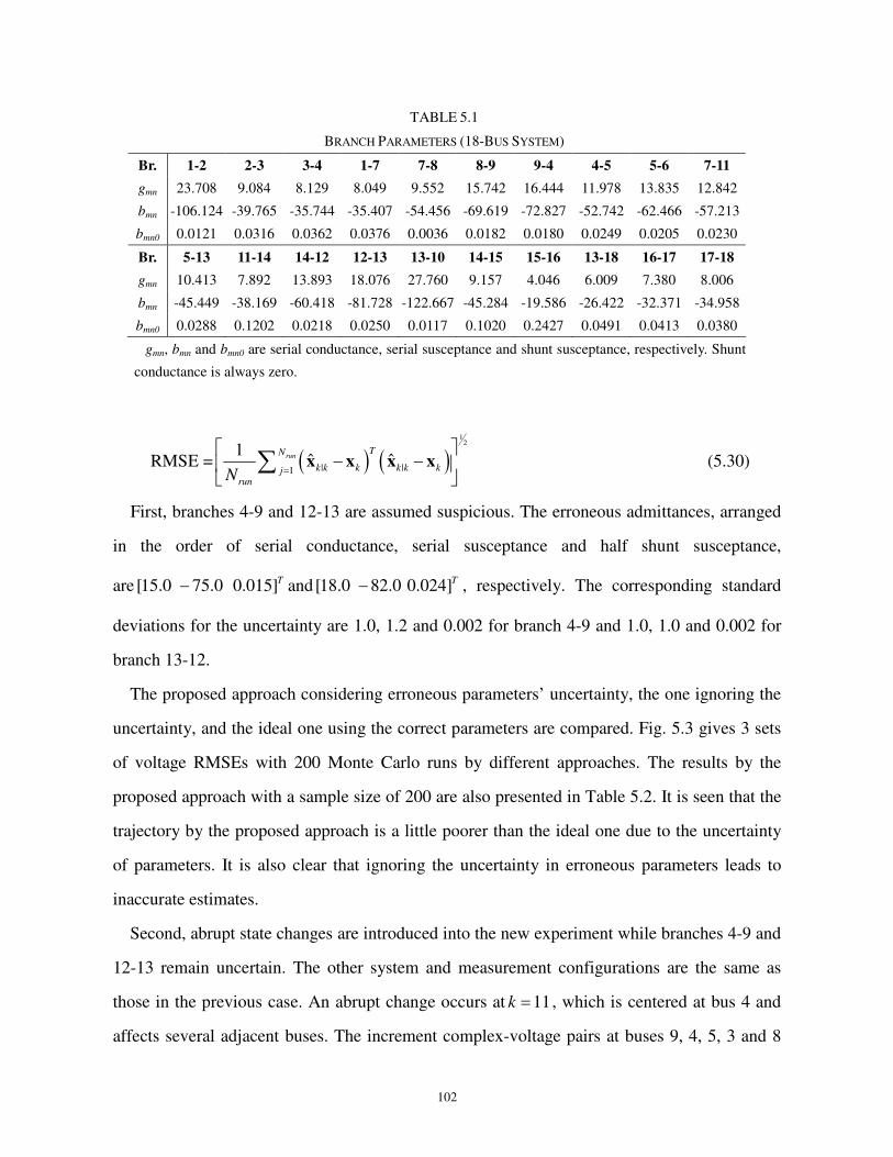
102
TABLE 5.1
BRANCH PARAMETERS (18-BUS SYSTEM)
Br. 1-2 2-3 3-4 1-7 7-8 8-9 9-4 4-5 5-6 7-11
gmn 23.708 9.084 8.129 8.049 9.552 15.742 16.444 11.978 13.835 12.842
bmn -106.124 -39.765 -35.744 -35.407 -54.456 -69.619 -72.827 -52.742 -62.466 -57.213
bmn0 0.0121 0.0316 0.0362 0.0376 0.0036 0.0182 0.0180 0.0249 0.0205 0.0230
Br. 5-13 11-14 14-12 12-13 13-10 14-15 15-16 13-18 16-17 17-18
gmn 10.413 7.892 13.893 18.076 27.760 9.157 4.046 6.009 7.380 8.006
bmn -45.449 -38.169 -60.418 -81.728 -122.667 -45.284 -19.586 -26.422 -32.371 -34.958
bmn0 0.0288 0.1202 0.0218 0.0250 0.0117 0.1020 0.2427 0.0491 0.0413 0.0380
gmn, bmn and bmn0 are serial conductance, serial susceptance and shunt susceptance, respectively. Shunt
conductance is always zero.
( ) ( )1
2
| |1
1ˆ ˆRMSE =
runTN
k k k k k kjrun
N =
− −
∑ x x x x (5.30)
First, branches 4-9 and 12-13 are assumed suspicious. The erroneous admittances, arranged
in the order of serial conductance, serial susceptance and half shunt susceptance,
are [15.0 75.0 0.015]T− and[18.0 82.0 0.024]T− , respectively. The corresponding standard
deviations for the uncertainty are 1.0, 1.2 and 0.002 for branch 4-9 and 1.0, 1.0 and 0.002 for
branch 13-12.
The proposed approach considering erroneous parameters’ uncertainty, the one ignoring the
uncertainty, and the ideal one using the correct parameters are compared. Fig. 5.3 gives 3 sets
of voltage RMSEs with 200 Monte Carlo runs by different approaches. The results by the
proposed approach with a sample size of 200 are also presented in Table 5.2. It is seen that the
trajectory by the proposed approach is a little poorer than the ideal one due to the uncertainty
of parameters. It is also clear that ignoring the uncertainty in erroneous parameters leads to
inaccurate estimates.
Second, abrupt state changes are introduced into the new experiment while branches 4-9 and
12-13 remain uncertain. The other system and measurement configurations are the same as
those in the previous case. An abrupt change occurs at 11k = , which is centered at bus 4 and
affects several adjacent buses. The increment complex-voltage pairs at buses 9, 4, 5, 3 and 8

103
are:
-0.02500 - 0.01745j , 0.04000 - 0.03490j , 0.02000 - 0.01396j ,
-0.01200 - 0.00872j , -0.01500 - 0.00872j
The change-detection threshold is 0.01α = . A simulation with 200 runs is conducted. The
RMSE results by the proposed one are in Table 5.3. Fig. 5.4 also shows two sets of voltage
RMSEs using the proposed state tracking and the one without detection and estimation of
change, respectively.
0 1 2 3 4 5 6 7 8 9 10 11 12 13 14 15 16 171
1.5
2
2.5
3
3.5
4
4.5
5x 10
-3
Time
RM
SE
(per
unit)
Ignored
Considered
Ideal
Fig. 5.3 Comparison on effect of parameter uncertainty
At 11k = , the values in the ‘Accounted’ trajectory are much smaller than those in the
‘Unaccounted’ one. In addition, at instants 5-10, the ‘Accounted’ values, which should
coincide with the ‘Unaccounted’, are still smaller. It implies that the change-detection-and-
estimation process has responded to false alarms, as discussed in Sec. 5.4.1. These
‘unexpected’ operations help improve the estimation accuracy. Thus it is shown that the

104
TABLE 5.2
RMSES OF FIRST EXPERIMENT (BY PROPOSED APPROACH)
Time 0 1 2 3 4 5 6 7 8
Value 0.00942 0.00210 0.00166 0.00191 0.00191 0.00200 0.00201 0.00177 0.00195
Time 9 10 11 12 13 14 15 16 17
Value 0.00205 0.00191 0.00184 0.00182 0.00176 0.00198 0.00186 0.00204 0.00170
TABLE 5.3
RMSES OF SECOND EXPERIMENT (BY PROPOSED APPROACH)
Time 0 1 2 3 4 5 6 7 8
Value 0.00910 0.00249 0.00246 0.00224 0.00246 0.00231 0.00213 0.00248 0.00220
Time 9 10 11 12 13 14 15 16 17
Value 0.00228 0.00212 0.00206 0.00207 0.00223 0.00223 0.00214 0.00217 0.00201
method of change detection and estimation is necessary and effective. In particular, in this
most complicated case, the average processing time for each prediction-update cycle (one
instant) is less than 0.05 second when the approach is implemented via MATLAB on a
computer with a single-core 3.0GHz CPU.
Third, the proposed approach accompanied by the newly-introduced dynamic model in (5.6)
is compared with a traditional approach using the random-walk model in (5.1) and an approach
using the forecasting model in (5.2). In the forecasting model, the coefficients F and G are
determined by the classic linear exponential smoothing method [Leite83].
The existing approaches do not consider the abrupt state changes and the possible uncertain
parameters, on which the proposed approach has already won out. To make a ‘fair’
comparison, only the case without abrupt changes and uncertain parameters is tested. All the
other system and measurement configurations are the same as those in the first test of Sec.
5.5.5. The RMSE trajectories by the proposed approach and the random-walk model based
approach are presented in Fig. 5.5. The plots indicate that the random-walk model leads to
results inferior to those by the proposed one.

105
0 1 2 3 4 5 6 7 8 9 10 11 12 13 14 15 16 172
2.2
2.4
2.6
2.8
3x 10
-3
Time
RM
SE
(per
unit)
Unaccounted
Accounted
Fig. 5.4 Comparison on effect of abrupt-state-change detection
0 5 10 15 201.5
2
2.5x 10
-3
Time
RM
SE
(per
unit)
RW
Exact
Fig. 5.5 Comparison with random-walk model
Fig. 5.6 plots the RMSE trajectories to compare the proposed approach with the forecasting
model based approach. The setting for the forecasting model is the same as that in [Leite83].
Clearly, the results are consistent with the analysis in Sec. 5.4.1 and the proposed approach has
better accuracy. In field applications, the PMU accuracy and the number of measurements may
not be as high as in the simulation setting, and it is also possible that some measured data are
not valid at some instants. In these realistic situations, the improved performance of the

106
proposed approach over the compared ones in Figs. 5.4, 5.5 and 5.6 will be more significant
since the estimation accuracy now relies more on the prediction model.
0 5 10 15 201.5
2
2.5x 10
-3
Time
RM
SE
(per
unit)
Forecasting
Exact
Fig. 5.6 Comparison with forecasting model
5.6 Conclusions
This chapter presents a novel approach to state tracking with correlated prediction-
measurement errors and possible abrupt state change. Prediction models have been analyzed,
leading to a new model. An adaptive filtering procedure, accompanied by detection and
estimation of abrupt changes, has been developed, which also considers the correlation
between the prediction and the pseudo measurement errors. Simulations illustrate the
performance of the approach under multiple conditions. High estimation accuracy is achieved
with this approach. In addition, the approach can be simplified and applied to conventional
DSE problems with synchrophasor data. It can also be introduced to other state estimation
problems with conventional SCADA data.
5.7 Appendices
5.7.1 Appendix A: Derivation of Filter on Correlated Errors and Noise
The linear system tracked by the standard Kalman filter (KF) usually assumes whiteness and
non-correlation. Reference [Li07] presents an optimal KF dealing with various correlations.
The following derivation, which follows [Li07] and adopts the predictor-corrector form of KF
[Bar-Shalom01] that is easy for implementation and coding, assumes that the prediction and

107
the measurement errors are correlated. For the system described by
1
1
, 1
k k k k
k k
c k k k
−−
−
= = + +
x 0 F M wx x
x 0 F M 0
( ( (5.31)
[ ]k k k k k k k= + = +z H x v H 0 x v( ( (
(5.32)
with M for a general input and w for zero-mean white noise, one predictor-corrector cycle (at
one time instant) of the filter includes prediction and update as follows.
1) Prediction:
The prediction is exactly the same as that in the standard KF. That is,
1| 11
| 1
, 1| 11
ˆˆ
ˆ
k kk k
k k
c k kk k
− −−−
− −−
= +
x0 F Mx
x0 F M
(
or | 1 , | 1 1 , 1| 1ˆ ˆ ˆ
k k c k k k c k k k− − − − −= = +x x F x M (5.33)
The corresponding mean-square error (MSE) matrix is
| 1 | 1 1 1| 1 1ˆcov( ) diag( , )T
k k k k k k k k k k− − − − − −= − = +P x x F P F Q 0( ( (( (
1 , 1| 1 1 1 , 1| 1 1
1 , 1| 1 1 1 , 1| 1 1
T T
k c k k k k k c k k k
T T
k c k k k k c k k k
− − − − − − − −
− − − − − − − −
+=
F P F Q F P F
F P F F P F
| 1 , | 1
, | 1 , | 1
k k c k k
c k k c k k
− −
− −
=
P P
P P
where cov( )⋅ is for covariance.
In other words,
| 1 , | 1
, | 1 1 , 1| 1 1
k k c k k k
T
c k k k c k k k
− −
− − − − −
= +
=
P P Q
P F P F (5.34)
2) Update:
The update includes the following steps similar to those in the standard KF.
The predicted measurement is
| 1 | 1 | 1ˆˆ ˆ
k k k k k k k k k k− − −= + = +z H x v H x v( (
(5.35)
where v is the mean of v . By definition, the innovation is
| 1ˆ
k k k k−∆ = −z z z (5.36)
108
The covariance of the innovation (assuming measurement-prediction-error correlation exits) is
| 1cov( ) ( )T T
k k k k k k k k k k k−= ∆ = + + +S z H P H R H A H A( (( ( ( ( (
| 1 ( )T T
k k k k k k k k k−= + + +H P H R H A H A (5.37)
where ( )T
k k k k+H A H A
( (( (is introduced by the newly-counted correlation. The filter gain is also
modified with kA(
. That is,
1
| 1( )T
k k k k k k
−−= +K P H A S
(( ( (
| 1 , | 1 1
, | 1 , | 1 ,
Tk k c k k kk
k
c k k c k k c k
− − −
− −
= +
P P AHS
P P A0
| 1 1
,, | 1 ,
T
kk k k k
kT
c kc k k k c k
− −
−
+ = = +
KP H AS
KP H A
In other words,
| 1
, , | 1 ,
T
k k k k k
T
c k c k k k c k
−
−
= +
= +
K P H A
K P H A (5.38)
Then the updated estimate and its MSE matrix are
| | , | | 1ˆ ˆˆ ˆ
TT T
k k k k c k k k k k k− = = + ∆ x x x x K z(( (
| 1
, | 1 ,
ˆ
ˆ
k k k
k
c k k c k
−
−
= + ∆
x Kz
x K (5.39)
| | | 1ˆcov( ) T
k k k k k k k k k k−= − = −P x x P K S K( ( ( (( (
| 1 , | 1
, | 1 , | 1 , ,
T
k k c k k k k
k
c k k c k k c k c k
− −
− −
= −
P P K KS
P P K K
| 1211 12
21 , |21 22
k k
c k k
= =
P DD D
D PD D (5.40)
with 11 | 1
T
k k k k k−= −D P K S K ,
21 , | 1 ,
T
c k k c k k k−= −D P K S K ,
12 , | 1 ,
T
c k k k k c k−= −D P K S K ,
and 22 , | 1 , ,
T
c k k c k k c k−= −D P K S K . In summary,

109
| | 1
, | , | 1 ,
| | 1
, | , | 1 , ,
ˆ ˆ
ˆ ˆ
k k k k k k
c k k c k k c k k
T
k k k k k k k
T
c k k c k k c k k c k
−
−
−
−
= + ∆
= + ∆
= − = −
x x K z
x x K z
P P K S K
P P K S K
(5.41)
5.7.2 Appendix B: Derivation of Abrupt Change Estimation
This derivation, inspired by the input estimation approach in [Bar-Shalom01], is based on
the model in (5.6). Hypotheses 0H and 1H are considered as follows.
1) 0H : 0k=u
According to (5.14), the prediction is
| 1 , 1| 1ˆ ˆ
k k c k k
− −− − −=x x (5.42)
Then the corresponding innovation is
, , , | 1ˆ
x k x k x k k k
− −−∆ = −z z H xo
, , , 1| 1ˆ
x k x k c k k
−− −= −z H xo (5.43)
2) 1H : 0k≠u ,
From (5.14), the prediction is
| 1 , 1| 1ˆ ˆ
k k c k k k− − −= +x x u (5.44)
The innovation under 1H is
, , , | 1ˆ
x k x k x k k k−∆ = −z z H xo
, , , 1| 1 ,ˆ
x k x k c k k x k k− −= − −z H x H uo o (5.45)
Comparing (5.43) with (5.45), and also considering the initial condition , 1| 1 , 1| 1ˆ ˆ
c k k c k kx−
− − − −=x , we
have
, , ,x k x k k x k
−∆ = + ∆z H u zo (5.46)
which implies that ,x k
−∆z and ,x k∆z form a measurement-and-noise pair with respect to
ku .
In the filter in Sec. 5.3, the covariancek
S does not depend on the concrete state values in the

110
filter. Thus ,x k
−∆z and ,x k∆z have the same covariance. Accordingly, the WLS estimate of
ku is
1 1 1
, , , ,ˆ [( ) ]T
k x k k x k x k k x kz− − − −=u H S H H S ∆
o o o (5.47)
111
Chapter 6: Joint Estimation of State and Parameter with
Synchrophasors—Part II: Parameter Tracking
6.1 Introduction
6.1.1 Previous Work
In more and more modern power systems, synchrophasors are deployed to meter bus
voltages directly, and branch-current phasors are also collected to maintain measurement
redundancy [Phadke02] [Martin08]. Consequently, accurate model parameters are required by
state estimators. Unfortunately, incorrect parameters exist and their percentage can be up to
30% in some utilities’ database [Kusic04]. Thus parameter estimation is crucial for power
system state estimation and other steady-state applications.
As surveyed by [Zarco00], parameter-estimation methods using residual sensitivity analysis
or augmenting the parameters into the state vector, with data from a single scan, have been
proposed [Liu92] [Liu95] [Alsac98]. These static-estimation methods are usually limited
because the measurement redundancy is inadequate in practice. Dynamic-estimation methods
using multi-scan data are generally preferred [Debs74]. They have better performance, but
require accurate dynamic models and relatively more computation. Typically, the dynamic
state vector is augmented [Debs74] [Slutsker96] and the extended Kalman filter (EKF) is
applied since the measurement functions are nonlinear. However, EKF-based approaches do
not perform well if the problems are highly nonlinear or some components of the augmented
state set are sensitive to measurement noise [Li04]. In addition, although several artificial
intelligent techniques have been introduced to improve prediction models in state estimation
[Sinha99] [Lin03] [Huang04], less attention has been paid to the dynamic behavior of the
involved voltages and parameters in parameter estimation. An inappropriate model may lead to
serious model mismatch errors, especially for filtering over a long period.

112
In essence, the EKF-based approaches (in power system state estimation) are industrial
applications of nonlinear filtering techniques which are largely classified into two categories:
point estimation and density estimation [Debs74]. In addition to EKF, other point estimation
methods, such as unscented filter [Julier04] and Gaussian filter [Ito00], employ different
approximation techniques to track nonlinear systems. Their performance is limited if the
specific system is not well approximated. Density-estimation methods, such as Fokker-Planck
equation based methods [Ahmed98] and particle filtering (PF) [Djuric03], try to provide exact
or approximate posterior probability density functions. However, they require sufficient
one-scan measurements and the computational requirements are demanding, especially in
high-dimensional cases.
For high-dimension low-redundancy nonlinear parameter estimation, we propose a balanced
method which adopts merits from both EKF and PF. It follows the simple structure of EKF but
further accounts for the uncertain effects such as involved bus voltages and high-order terms
(of Taylor’s expansion) in EKF as the pseudo measurement errors correlated with the
prediction errors. Correspondingly, a recently-developed optimal filtering technique that can
handle correlation [Li07] is introduced (see Chapter 5). We also introduce random samples
from the idea of PF to evolve the pseudo-error ensembles and to evaluate the statistics related
to the pseudo errors, where the error-ensemble sampling does not rely on the measurement
redundancy and is much easier to implement than PF. Based on this balanced method, the joint
state-and-parameter estimation considering complicated behaviors of voltages and parameters
is discussed.
6.1.2 Our Contributions
The problem of parameter estimation with synchrophasor data is formulated as two
loosely-coupled subproblems: state tracking (presented in Chapter 5) and parameter tracking.
This chapter focuses on the parameter tracking, where only line parameters are estimated and
the involved bus voltages are now treated as uncertain “measurement- function coefficients”.
The work includes:

113
1) A new prediction model accounting for the effect of prior knowledge and moving
parameter means is proposed. The measurement model is also improved by introducing a
concept of pseudo measurement error to cover the uncertainty in the estimated voltages,
high-order terms and measurement errors.
2) An adaptive filter is developed, based on the optimal filtering with correlated
prediction-measurement errors.
3) A sliding-window method is proposed to detect the moving tendency of parameters and
adjust the transition matrix adaptively. It is embedded in the adaptive filter.
4) A sample-based method, namely, error-ensemble evolution, is used to evaluate the
correlation between pseudo measurement errors and prediction errors.
5) In addition, a refinery-and-adaptation method is suggested for the use of realistic systems
where the data-acquisition rate is high. Specifically, with the above setting, parameters from
different lines can be accurately calibrated in parallel.
In particular, the work of this chapter has been published in [Bian11b].
6.2 Parameter Estimation
The goal is to calibrate the steady-state parameters in the -typeπ equivalent circuits
(Pi-Model) of transmission lines using multi-scan synchrophasor data. The bus voltages at the
nodes connected by these lines, which are included in the measurement function, also need to
be determined. To obtain accurate estimates of the two voltages, a few adjacent buses usually
are involved. Accordingly, the overall measurement equation can be written as
( , )k k k k= +z h x p v (6.1)
where
z vector of measurements forp and x
p vector of admittance over to-be-calibrated lines, e.g., admittance of a single line
(by the -typeπ circuit) is [ ]0 0 T
mn mn mn mng g b b

114
mng serial conductance in the -typeπ circuit for a line connecting nodes m and n
0mng half shunt conductance in the -typeπ circuit for a line connecting nodes m and n
mnb serial susceptance of the -typeπ circuit for a line connecting nodes m and n
0mnb half shunt susceptance of the -typeπ circuit for a line connecting nodes m and n
x bus voltages
( )⋅h function (set) relatingp and x with measurements
v vector of measurement noise
In conventional parameter estimation, p and x are solved as an augmented state, which leads
to a typical nonlinear estimation problem and estimation accuracy is not guaranteed. We
formulate this problem as two loosely-coupled subproblems: state tracking and parameter
tracking, incorporated by an error-ensemble-evolution method dealing with the coupling. In
one (state or parameter) tracking procedure, the other estimand (p or x ) is taken as uncertain
“coefficients” in measurement function related to the current one. Consequently, the dynamic
behaviors of the state and the parameters are studied separately since they do act differently in
reality and the effect of the uncertain coefficients is represented by pseudo measurement
errors. Specific filters are also developed. Specifically, in parameter tracking, the measurement
set includes the involved branch-current data only and each current phasor pair is exclusively
incident to one branch. This implies that parameters from different lines can be calibrated
separately.
The state tracking has been presented in Chapter 5. This chapter discusses the overall
approach and focuses mainly on the adaptive parameter tracking with uncertain voltages and
the method to evaluate the involved correlation.
6.3 Formulation of Parameter Tracking
As discussed in Sec. 6.2, admittances from different transmission lines can be processed in
parallel. Thus, a single transmission line is considered in the subsequent discussion.

115
6.3.1 Prediction Model
The dynamic behavior of line parameters is modeled as
, ,
, , 1( , )
k c k p k
c k c kf k−
= +
=
p p w
p p (6.2)
where
cp mean (center) of p
pw vector of zero-mean process noise in p , caused by small disturbances (e.g., wind or
rain)
( )f ⋅ function for deterministic moving tendency ofc
p
This prediction model emphasizes two facts: (a) rather than a random walk, the true values
vary randomly around a deterministic “center”; (b) the center is not necessarily constant. It
may move over time since the transmission line can shrink or expand from heat, moisture, etc.
Specifically, an adaptive model is utilized to approximate this moving tendency:
, , 1 , 1c k p k c k− −=p F p , (6.3)
where transition matrixp
F is adjusted by the sliding-window method (see Sec. 6.4.2).
6.3.2 Measurement Model
The voltages have been estimated using the scheme presented in Chapter 5. Thus only the
synchronized branch currents through the to-be-calibrated line are considered in the
measurement set. All the data are in the rectangular form. For those synchrophasors providing
data in the angular-form only, the coordinate transformation used in [Bi08] can be employed to
preprocess the data. The measurement model is
, , ,p k p k k p k= +z H p v , (6.4)
where

116
, , , , , ,
, , , , , ,
,
, , , , , ,
, , , , , ,
r m r n i n i m r m i m
i m i n r m r n i m r m
p k
r n r m i m i n r n i n
i n i m r n r m i n r n k
x x x x x x
x x x x x x
x x x x x x
x x x x x x
− − − − − = − − −
− −
H (6.5)
pz vector of branch-current measurements
pv vector of branch-current measurement noise
x entry of x
Note that (6.5) is for two pairs of complex branch currents in reverse directions. For more
redundant current observations, (6.5) will be extended. Furthermore, since notk
x but its
estimate ˆk
x is available, (6.4) is refined as
, , ,p k p k k p k= +z H p vo o , (6.6)
where ,p kHo is a coefficient matrix obtained from ,p kH by replacing
kx with ˆ
kx . The pseudo
measurement noise is
, , | 1 | 1 ,ˆ( )p k p k k k k k p k− −= ∆ + ∆ +v H p p vo , (6.7)
where | 1ˆ
k k−p is predicted estimate of p . | 1 | 1ˆ
k k k k k− −∆ = −p p p , , , ,p k p k p k∆ = −H H Ho , and ,p k∆H
depends on ˆk k k
∆ = −x x x .
The updated estimate |ˆ
k kx is used as ˆ
kx in this chapter. The process and (original)
measurement noises are assumed zero-mean, white Gaussian, and mutually independent.
6.4 Tracking of Line Parameters
6.4.1 Basic Filter
The adaptive filter for the parameter tracking is arranged in the predictor-corrector form and
includes recursive steps as below (also see Fig. 6.1).
1) Initialization: 0k =
0|0 ,0|0ˆ ˆ
c=p p ; 0|0 ,0|0 c=P P% % (6.8)
117
2) Recursion: : 1k k= +
Determine , 1p k−F (see Sec. 6.4.2)
Prediction:
| 1 , | 1ˆ ˆ
k k c k k− −=p p ; , | 1 , 1 , 1| 1ˆ ˆ
c k k p k c k k− − − −=p F p (6.9)
| 1 , | 1 ,
, | 1 , 1 , 1| 1 , 1
k k c k k p k
T
c k k p k c k k p k
− −
− − − − −
= +
=
P P Q
P F P F
% %
% % (6.10)
, | 1 , | 1 ,ˆˆ
p k k p k k k p k− −= +z H p vo o (6.11)
Update:
, | 1 , , , ,
T T T
k p k k k p k p k p k k k p k−= + + +S H P H R H A A Ho o o o o% % %% (6.12)
( )( )
1
| 1 ,
1
, , | 1 , ,
T
k k k p k k k
T
c k c k k p k c k k
−−
−−
= +
= +
K P H A S
K P H A S
o
o
% %% %
% %% % (6.13)
, , , | 1ˆ
p k p k p k k−∆ = −z z z (6.14)
Finally,
| | 1 ,
, | , | 1 , ,
ˆ ˆ
ˆ ˆ
k k k k k p k
c k k c k k c k p k
−
−
= + ∆
= + ∆
p p K z
p p K z
%
% (6.15)
| | 1
, | , | 1 , ,
T
k k k k k k k
T
c k k c k k c k k c k
−
−
= −
= −
P P K S K
P P K S K
%% % % %
%% % % % (6.16)
Here,
P% covariance of estimation error in p
cP% covariance of estimation error in ˆ
cp
The following quantities are assumed known:
pQ covariance of parameter process noise
pw
pR covariance of original measurement noise
pv

118
In addition, the mean and covariance of ,p kvo ( pvo and pRo ), and the correlation between the
prediction and the pseudo measurement errors which includes
| 1 ,cov( , )k k k p k−= ∆A p vo% , (6.17)
, , | 1 ,cov( , )c k c k k p k−= ∆A p vo% , (6.18)
should be preprocessed. It is discussed in detail in Sec. 6.5.
6.4.2 Adjustment of Transition Matrix
Detection of the moving tendency in the parameter center is based on the following fact: As
opposite to that the mismatched prediction model drives the predicted values farther and
farther away, the newly-arrived measurements tend to pull the updated values back toward the
truth. Consequently, a sliding-window method based on evidence from detN successive instants
is proposed, which contains two hypotheses as
0H : The center keeps increasing in the current window;
1H : The center keeps decreasing in the current window.
In the case that neither 0H nor 1H is correct, the center is assumed to remain constant in the
current window.
pF is usually assumed diagonal and all the diagonal elements can be adjusted in a similar
way. Let p be a representative element in p andp
f be the corresponding diagonal entry ofp
F ,
respectively. Three decision rules are designed as follows:
1) Decide 0H if | | 1ˆ ˆ 1
k k k kp p − > occurs at least 1
0 det2N N+ times within a window of swN
instants.
2) Decide 1H if | | 1ˆ ˆ 1
k k k kp p − < occurs at least 1
1 det2N N+ times within the current window.
3) Slide the window forward by one step if neither 0H nor 1H is decided.
119
To obtain a smooth parameter-tracking trajectory, we propose a scheme to tunep
f after
either 0H or 1H is declared:
a) 0N and 1N can be set equal, and a small value such as 1, 2 and 3 can be used;
b) detN is preset according to field experience (by observing the tracking trajectory);
c) Past data can be used to reduce the false-alarm probability and eliminate possible delay.
That is, an adjustment window may have adjN ( detN> ) instants. If 0H (or 1H ) still holds within
the adjustment window, continue tuningp
f ; otherwise, end and move the detection window.
d) In the adjustment window, p
f is turned up (or down) conservatively. For instance, if
| | 1ˆ ˆ 1
k k k kp p − > occurs tempN ( 1
0 det2N N≥ + ) times,
pf should be turned up until tempN is reduced
by 1. This stop criterion is milder than those in 0H and 1H . In addition, the calculated prediction
covariance at the first instant of the window is multiplied byβ ( 1.0> ) , which assigns more
weight to the data than to the prediction since the prediction model is detected to be inaccurate.
In fact, the introduction of 0N , 1N , detN , adjN , and β makes the adjustment flexible to
handle. The well-fitted trajectory is expected to be smooth. Otherwise, when the tunedp
f
vibrates frequently, 0N and 1N have to be turned up to reduce the false-alarm probability; when
pf does not vibrate frequently but has abrupt increments, 0N and 1N have to be turned down to
reduce the missing probability.
6.5 Error Evolution and Correlation Calculation
This section deals with the coupling between the state tracking and the parameter tracking.
Specifically, it calculates pvo , pRo , A% andc
A% . It also evaluatesx
vo , A ,
cA and
xR
o for the state
tracking in Chapter 5. We will not calculate the above quantities analytically. An
error-ensemble-evolution method is used to evaluate them numerically. The main ideas

120
include: (i) evolve the ensemble of estimation errors for the coupled state and parameter via
error evolution; (ii) combine two sets of error samples to get the ensemble of pseudo errors;
and (iii) evaluate the relevant quantities.
Details of the error evolution are given in the Appendix. The correlation calculation consists
of the following steps:
First, perform initialization: 0k =
a) Obtain ( )
,0|0
j
c∆x by sampling from ,0|0(0, )c
N P
b) Obtain ( )
,0|0
j
c∆p by sampling from ,0|0(0, )cN P%
Second, begin recursion:
1) Set : 1k k= +
2) Obtain ( )
,
j
x kvo when | 1ˆ
k k−p and | 1ˆ
k k−x are ready:
a) Obtain ( )
,
j
p kw by sampling from ,(0, )p k
N Q
b) Evolve
( ) ( )
, | 1 , 1 , 1| 1
( ) ( ) ( )
| 1 , | 1 ,
j j
c k k p k c k k
j j j
k k c k k p k
− − − −
− −
∆ = ∆∆ = ∆ +
p F p
p p w
c) Obtain ( )
,
j
x kw by sampling from ,(0, )x k
N Q
d) Evolve
( ) ( )
, | 1 , 1| 1
( ) ( ) ( )
| 1 , | 1 ,
j j
c k k c k k
j j j
k k c k k x k
− − −
− −
∆ = ∆∆ = ∆ +
x x
x x w
e) Obtain ( )
,
j
x kv by sampling from ,(0, )x k
N R
f) Obtain ( ) ( ) ( ) ( )
, , | 1 | 1 ,ˆ( )j j j j
x k x k k k k k x k− −= ∆ + ∆ +v H x x vo , where ( )
,
j
x k∆H only depends on ( )
| 1
j
k k−∆p
3) Calculate
( )
, ,
1 j
x k x kjsample
N= ∑v vo o (6.19)
( ) ( )
, , , , ,
1( )( )j j T
x k x k x k x k x kjsample
N= − −∑R v v v vo o o o o (6.20)

121
( ) ( )
| 1 , ,
1( )j j T
k k k x k x kjsample
N−= ∆ −∑A x v vo o (6.21)
( ) ( )
, , | 1 , ,
1( )j j T
c k c k k x k x kjsample
N−= ∆ −∑A x v vo o (6.22)
4) Obtain ( )
,
j
p kvo when | 1ˆ
k k−p and |ˆ
k kx are ready:
a) Update ( )
|
j
k k∆x via error evolution
( ) ( ) ( )
, | 1 , ,
j j j
k x k k k x k x k−∆ = ∆ + −z H x v vo o o
( ) ( ) ( )
, | , | 1 ,
( ) ( ) ( )
| | 1
j j j
c k k c k k c k k
j j j
k k k k k k
−
−
∆ = ∆ − ∆∆ = ∆ − ∆
x x K z
x x K z
b) Obtain ( ) ( ) ( ) ( )
, , | 1 | 1 ,ˆ( )
j j j j
p k p k k k k k p k− −= ∆ + ∆ +v H p p vo o , where ( )
,
j
p k∆H
o depends only on ( )
|
j
k k∆x , and ( )
,j
p kv is a
part of ( )
,
j
x kv
5) Calculate
( )
, ,
1 j
p k p kjsample
N= ∑v vo o , (6.23)
( ) ( )
, , , , ,
1( )( )j j T
p k p k p k p k p kjsample
N= − −∑R v v v vo o o o o (6.24)
( ) ( )
| 1 , ,
1( )j j T
k k k p k p kjsample
N−= ∆ −∑A p v vo o% (6.25)
( ) ( )
, , | 1 , ,
1( )j j T
c k c k k p k p kjsample
N−= ∆ −∑A p v vo o% (6.26)
6) Update ( )
|
j
k k∆p
( ) ( ) ( )
, | 1 , ,
j j j
k p k k k p k p k−∆ = ∆ + −z H p v vo o o (6.27)
( ) ( ) ( )
, | , | 1 ,
( ) ( ) ( )
| | 1
j j j
c k k c k k c k k
j j j
k k k k k k
−
−
∆ = ∆ − ∆∆ = ∆ − ∆
p p K z
p p K z
%
% (6.28)

122
Here the recursion ends if k reaches the maximum number. j is the sample index, sample
N
the total sample size, and ( )N ⋅ Gaussian probability density function.
6.6 Procedures and Performance Analysis
6.6.1 Parameter Tracking and Overall Procedure
We have presented three major components of the joint state and parameter estimation.
From the viewpoint of parameter tracking, the estimated voltages are uncertain “measurement
coefficients” and the uncertainty is represented by pseudo measurement errors. A similar
strategy holds when discussed from the viewpoint of state tracking. The error ensemble keeps
evolving errors for the evaluation of the statistics related to pseudo errors in both tracking
procedures.
Furthermore, the dynamic behaviors of the voltages and the parameters are different. The
former may jump abruptly while the latter may increase (or decrease) slowly but persistently.
Correspondingly, appropriate detection and adaptation techniques have been developed.
The overview for the joint state-and-parameter estimation is depicted in Fig. 6.1. The
proposed method consists of parameter-tracking, state-tracking (in Chapter 5) and
correlation-calculation. The parameter tracking procedure is located on the left side.
6.6.2 Accuracy and Complexity
The filtering is based on the newly-developed optimal Kalman filter considering
prediction-measurement-error correlation. When the parameter center moves persistently, the
adaptation mechanism works out (not necessarily optimal yet) accurate results.
In practice, several detailed modules can still be simplified to save computation. For
instance, when estimation errors of parameters are large, the related branch-current
measurements contribute little to the state tracking. If the one-scan measurement redundancy
allows, the currents can be discarded temporarily to simplify the ensemble evolution.
Based on the fact that the calibration of the serial and shunt admittance of a transmission
line only involves the incident branch currents and the bus voltages at two ends, parameters of
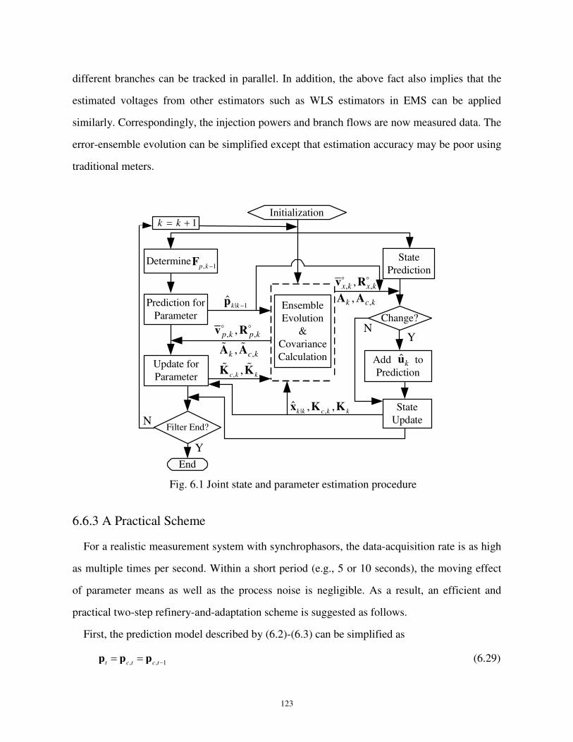
123
different branches can be tracked in parallel. In addition, the above fact also implies that the
estimated voltages from other estimators such as WLS estimators in EMS can be applied
similarly. Correspondingly, the injection powers and branch flows are now measured data. The
error-ensemble evolution can be simplified except that estimation accuracy may be poor using
traditional meters.
Determine
Update for
Parameter
Filter End?
Y
End
N
| 1ˆ
k k−p
1k k= +
, ,,p k p kv Ro o
,,k c kA A% %
Prediction for
Parameter
, 1p k−F
Ensemble
Evolution
&
Covariance
Calculation
Change?
State
Prediction
Add to
Prediction
State
Update
YN
Initialization
| ,ˆ , ,k k c k kx K K
ˆku
, ,,x k x kv Ro o
,,k c kA A
, ,c k kK K% %
Fig. 6.1 Joint state and parameter estimation procedure
6.6.3 A Practical Scheme
For a realistic measurement system with synchrophasors, the data-acquisition rate is as high
as multiple times per second. Within a short period (e.g., 5 or 10 seconds), the moving effect
of parameter means as well as the process noise is negligible. As a result, an efficient and
practical two-step refinery-and-adaptation scheme is suggested as follows.
First, the prediction model described by (6.2)-(6.3) can be simplified as
, , 1t c t c t−= =p p p (6.29)

124
The (simplified) basic filter and error-ensemble evolution can be utilized to roughly
estimatep using data within each period, where the filter is reinitialized at each first instant to
release the dependence on the previous period. Second, |ˆ
t tp and |t tP% at the last instant of each
period can be treated as the refined data and put into the adaptive filter (including the
adaptation mechanism) with the model
, ,
, , 1 , 1
k c k p k
c k p k c k− −
= +
=
p p w
p F p (6.30)
At this step, |ˆ
t tp are direct “measurement” of
kp and no correlation calculation is needed.
6.7 Simulations
The purposes are to show the performance of the parameter tracking, the effectiveness of the
correlation calculation, and the performance of the overall approach. Tests were carried out on
a realistic system for comparison. In the tests, the system states and to-be-determined
parameters at different times were simulated by adding zero-mean Gaussian noise to the
base-case network data. The synchronously-measured data were also generated in this way.
6.7.1 Comparisons with Other Approaches
The proposed approach is compared with an improved EKF approach and an ideal approach
to be explained next.
In the standard EKF approach, the predicted values of the augmented state (voltages and
parameters) are used in the Jacobian matrix during the linearization. In this example, it is
improved by a stepwise strategy which estimates the voltages and the parameters one by one.
Then the updated voltages are available to the Jacobian matrix in the parameter tracking.
In the ideal approach, the system state is assumed to be known “perfectly”, which is not
feasible in practice but provides a reference for comparison.
The experiment is on a realistic system depicted in Fig. 6.2. This system is a 550kV bulk
network supplying power for a major city in China. The line parameters are listed in Table 6.1.
Bus 1 is the reference bus. The standard deviations of the real and imaginary voltage process
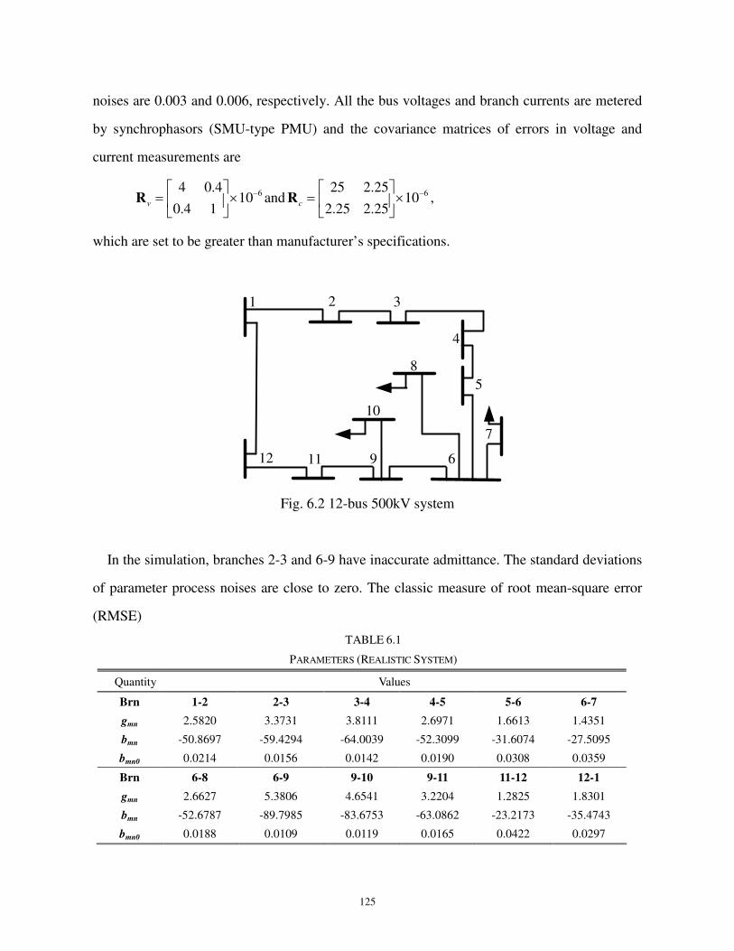
125
noises are 0.003 and 0.006, respectively. All the bus voltages and branch currents are metered
by synchrophasors (SMU-type PMU) and the covariance matrices of errors in voltage and
current measurements are
64 0.4
100.4 1
v
− = ×
R and 625 2.25
102.25 2.25
c
− = ×
R ,
which are set to be greater than manufacturer’s specifications.
1 2 3
4
5
6
7
8
9
10
1112
Fig. 6.2 12-bus 500kV system
In the simulation, branches 2-3 and 6-9 have inaccurate admittance. The standard deviations
of parameter process noises are close to zero. The classic measure of root mean-square error
(RMSE)
TABLE 6.1
PARAMETERS (REALISTIC SYSTEM)
Quantity Values
Brn 1-2 2-3 3-4 4-5 5-6 6-7
gmn 2.5820 3.3731 3.8111 2.6971 1.6613 1.4351
bmn -50.8697 -59.4294 -64.0039 -52.3099 -31.6074 -27.5095
bmn0 0.0214 0.0156 0.0142 0.0190 0.0308 0.0359
Brn 6-8 6-9 9-10 9-11 11-12 12-1
gmn 2.6627 5.3806 4.6541 3.2204 1.2825 1.8301
bmn -52.6787 -89.7985 -83.6753 -63.0862 -23.2173 -35.4743
bmn0 0.0188 0.0109 0.0119 0.0165 0.0422 0.0297

126
( ) ( )1
2
| |
1
1ˆ ˆRMSE =
runNT
k k k k k k
jrunN =
− −
∑ p p p p (6.31)
is adopted, whererun
N is the total number of Monte-Carlo runs.
The resultant trajectories averaged over 200 runs are plotted in Fig. 6.3. It shows that the
proposed approach is much better than the improved EKF approach. The RMSE values from
the proposed approach converge faster. The difference between the proposed and the ideal
trajectories, caused by the uncertainty in the state estimates, is not large.
0 10 20 30 40 50 600
0.2
0.4
0.6
0.8
1
Time
RM
SE
Proposed
Ideal
EKF
Fig. 6.3 Performance comparison with EKF
6.7.2 Practical Two-Step Implementation of the Approach
This part contains a particular test on the practical refinery-and-adaptation scheme discussed
in Sec. 6.6.3. The experiment is implemented on the realistic system in Fig. 6.2, where the
centers of line parameters move persistently. All the other system and measurement
configurations are the same as those in Sec. 6.7.1. The data-acquisition rate is 5 times per
second, and the observation interval covers 25 minutes. That is, 7500 pieces of data are
recorded. Specifically, the line parameter in branch 6-9 moves at rates of 0.99999, 0.99997 and
0.99998 over intervals 1500-3200, 3201-4600 and 4601-6000, respectively.
First, the parameters are refined every 20 instants by the simplified tracking procedure using
the model (6.29) and the error ensemble evolution method. Second, the simplified adaptive

127
tracking procedure with the model (6.30) is applied with the 375 pieces of refined data. The
lengths of windows are det 20N = and adj 30N = , respectively. The thresholds are 0 1 2N N= = .
The amplification rate is 1.02β = . In contrast, another tracking procedure ignoring the
possible center moving is also applied.
Fig. 6.4 plots the comparison results by the two approaches. In practice, the ratio of
estimation errors to the true values may also be interested. As a result, the RMSE measure
defined in (6.31) is modified: each component of |ˆ
k k k−p p is divided by the corresponding true
value and the eventual result is averaged over the components. Fig. 6.5 is a zoomed-in version
of Fig. 6.4. Clearly, the ‘Proposed’ trajectory can reach as low as 0.2% and is significantly
better than the ‘Ignored’ one.
In addition, the processing time is less than 0.01 second per instant on a computer with a
single-core 3.0GHz CPU.
1000 2000 3000 4000 5000 6000 70000
0.02
0.04
0.06
Time
Modifie
d R
MS
E
Proposed
Ignored
Fig. 6.4 Practical scheme based on 12-bus system
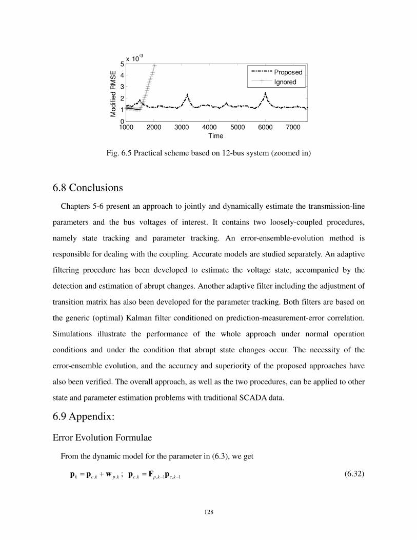
128
1000 2000 3000 4000 5000 6000 70000
1
2
3
4
5x 10
-3
Time
Modifie
d R
MS
E
Proposed
Ignored
Fig. 6.5 Practical scheme based on 12-bus system (zoomed in)
6.8 Conclusions
Chapters 5-6 present an approach to jointly and dynamically estimate the transmission-line
parameters and the bus voltages of interest. It contains two loosely-coupled procedures,
namely state tracking and parameter tracking. An error-ensemble-evolution method is
responsible for dealing with the coupling. Accurate models are studied separately. An adaptive
filtering procedure has been developed to estimate the voltage state, accompanied by the
detection and estimation of abrupt changes. Another adaptive filter including the adjustment of
transition matrix has also been developed for the parameter tracking. Both filters are based on
the generic (optimal) Kalman filter conditioned on prediction-measurement-error correlation.
Simulations illustrate the performance of the whole approach under normal operation
conditions and under the condition that abrupt state changes occur. The necessity of the
error-ensemble evolution, and the accuracy and superiority of the proposed approaches have
also been verified. The overall approach, as well as the two procedures, can be applied to other
state and parameter estimation problems with traditional SCADA data.
6.9 Appendix:
Error Evolution Formulae
From the dynamic model for the parameter in (6.3), we get
, ,k c k p k= +p p w ; , , 1 , 1c k p k c k− −=p F p (6.32)

129
According to (6.9), the prediction at time k is
| 1 , | 1 , 1 , 1| 1ˆ ˆ ˆ
k k c k k p k c k k− − − − −= =p p F p . (6.33)
Then the prediction errors are
, | 1 , , | 1ˆ
c k k c k c k k− −∆ = −p p p , 1 , 1 , 1| 1ˆ( )
p k c k c k k− − − −= −F p p
, 1 , 1| 1p k c k k− − −= ∆F p , (6.34)
| 1 | 1ˆ
k k k k k− −∆ = −p p p
, , , | 1 , | 1 ,ˆ
c k p k c k k c k k p k− −= + − = ∆ +p w p p w . (6.35)
From (6.15) and (6.16), the updated parameters at time k is
| | 1 ,
, | , | 1 , ,
ˆ ˆ
ˆ ˆ
k k k k k p k
c k k c k k c k p k
−
−
= + ∆
= + ∆
p p K z
p p K z
%
%. (6.36)
Then the corresponding estimation errors are
| |ˆ
k k k k k∆ = −p p p | 1 ,
ˆk k k k p k−= − − ∆p p K z% ( )| 1 , | 1 ,
ˆ ˆk k k k p k p k k p k− −= − − − −p p K z H p vo o%
( )| 1 , | 1 ,ˆ
k k k p k p k p k k p k− −= ∆ − + − −p K H p v H p vo o o o%| 1 | 1 , ,( )k k k p k k p k p k− −= ∆ − ∆ + −p K H p v vo o o%
( ), | , | 1 , | 1 , ,ˆ
c k k c k k c k p k k p k p k− −∆ = ∆ − ∆ + −p p K H p v vo o o%
In summary,
( )
, | 1 , 1 , 1| 1
| 1 , | 1 ,
, | , | 1 , | 1 , ,
| | 1 | 1 , ,( )
c k k p k c k k
k k c k k p k
c k k c k k c k p k k p k p k
k k k k k p k k p k p k
− − − −
− −
− −
− −
∆ = ∆∆ = ∆ +∆ = ∆ − ∆ + −∆ = ∆ − ∆ + −
p F p
p p w
p p K H p v v
p p K H p v v
o o o
o o o
%
%
(6.37)
Similarly, for the bus-voltage state in Chapter 5, we can get
( )
, | 1 , 1| 1
| 1 , | 1 ,
, | , | 1 , | 1 , ,
| | 1 | 1 , ,( )
c k k c k k
k k c k k x k
c k k c k k c k x k k x k x k
k k k k k x k k x k x k
− − −
− −
− −
− −
∆ = ∆∆ = ∆ +∆ = ∆ − ∆ + −∆ = ∆ − ∆ + −
x x
x x w
x x K H x v v
x x K H x v v
o o o
o o o
(6.38)

130
Chapter 7: Summary and Future Work
The least-squares (LS) principle, including the weighted least-squares (WLS), is widely
introduced to various scientific and technological fields. A great many methods have been
developed to solve the fundamental and classic LS problem, among which the
matrix-inversion-lemma based recursive least-squares (RLS) is a milestone. The RLS is of
recursive form and free of matrix inversion, and thus has excellent performance regarding the
efficient real-time computation and low memory storage. We generalize the RLS procedure
and to solve the unconstrained/ LE-constrained generalized LS (GLS) problem in a similar
recursive way. We also apply the RLS method for all the involved initializations. The
newly-developed methods are integrated as completely-recursive LS (CRLS).
Correspondingly, in Chapter 2, the generalization of the RLS for solving GLS problems is
discussed. Concretely, starting from the unconstrained/LE-constrained RLS, we develop
recursive procedures applicable to the unconstrained/LE-constrained GLS, and show that the
LE constraint is in essence a set of special observations free of observation errors and can be
processed sequentially in any place in the data sequence. More generally, we also treat the
ILE-constrained GLS. A unified recursive procedure is developed, which is applicable to
ILE-constrained GLS as well as all the unconstrained/LE-constrained LS/WLS/GLS.
In Chapter 3, a recursive exact initialization applicable to all the RLS, RWLS and RGLS, is
investigated. This chapter treats the RLS initialization-related issues, including rank check, a
convenient method to compute the involved matrix inverse/pseudoinverse, and resolution of
underdetermined systems. No extra non-RLS formula but an auxiliary-observation based
procedure is utilized. The RLS recursion can start from the first real observation and possible
LE constraints are also imposed recursively; the rank of the system is checked implicitly. If the
rank is full, the initialization and the subsequent RLS cycles can be integrated as a whole to
yield exact LS solutions. If the rank is deficient, the procedure provides a mapping from the
unobservable (original) estimand to a reduced-dimensional set of alternative variables which

131
are linear combinations of the original variables and uniquely determined. The consequent
estimate is a set of refined non-redundant observations. The refinement is lossless in the WLS
sense: if new observations are available later, it can take the role of the original data in the
recalculation.
In summary, the CRLS approach has the following good properties: The proposed method
can distribute the processing time (including the initialization) over the data-accumulation
period; The CRLS has a low computational complexity; With the CRLS, the initialization of
LE-constrained RLS solution, which (in the batch form) usually involves MP inverses, is made
as simple as for the unconstrained ones now; In sparse applications, the CRLS can benefit
more from the sparsity because its recursion can make full use of the sparse structure of the
observation coefficients; The observability analysis in the CRLS requires no extra
computation. The result by the CRLS is numerically consistent with the existence ofC in
calculation.
In Chapter 4, we demonstrate the mathematical equivalence between the linear-data-model
based linear minimum-mean-square-error (LMMSE) estimator and the ILE-constrained GLS.
We also suggest to use the recursive ILE-constrained GLS to improve the sequential procedure
of the optimal KF considering prediction-measurement-error correlation.
In Chapters 5 & 6, we perform accurate parameter (and state) estimation in complex
situations using synchrophasor data, based on the optimal KF considering the correlation
between the measurement noise and the prediction error. An approach of joint
state-and-parameter estimation, which is different from the state augmentation, is adopted,
where the original nonlinear PE problem is reformulated as two loosely-coupled linear
subproblems: state tracking and parameter tracking, respectively.
An error-ensemble-evolution method is responsible for dealing with the coupling between
the state tracking and the parameter tracking. Accurate models are studied separately. An
adaptive filtering procedure has been developed to estimate the voltage state, accompanied by
the detection and estimation of abrupt changes. Another adaptive filter including the

132
adjustment of transition matrix has also been developed for the parameter tracking. Both filters
are based on the optimal KF conditioned on prediction-measurement-error correlation.
Simulations illustrate the performance of the whole approach under normal operation
conditions and under the condition that abrupt state changes occur. The necessity of the
error-ensemble evolution, and the accuracy and superiority of the proposed approaches have
also been verified. The overall approach, as well as the two procedures, can be applied to other
state and parameter estimation problems with traditional SCADA data.
As declared in this dissertation, we have great interest in applying the newly-developed
CRLS approach to solve practical applications. For instance, the joint-state-and-parameter
estimation in power system based on synchrophasors is an application of the optimal KF
considering prediction-measurement-error correlation, where the filter can be verified and the
corresponding sequential procedure can be improved by the CRLS. In the future, we also aim
to utilizing the proposed recursive RLS initialization technique to solve high-dimensional and
low-redundancy practical problems. For instance, the application to power system state
estimation with synchrophasors is quite attractive.
133
References
[001] A. Abur and A. G. Exposito, Power System State Estimation: Theory and Implementation, Marcel Dekker,
NY, 2004
[002] N. U. Ahmed, Linear and Nonlinear Filtering for Scientists and Engineers, World Scientific, Singapore,
1998
[003] A. Albert and R. W. Sittler, “A method for computing least squares estimators that keep up with the data,”
SIAM Journal on Control and Optimization, vol. 3, no. 3, pp. 384-417, 1965
[004] O. Alsac, N. Vempati, B. Stott, and A. Monticelli, "Generalized state estimation," IEEE Trans. Power Syst.,
vol. 13, no.3, pp. 1069-1075, Aug. 1998
[005] T. Amemiya, Advanced Econometrics, Cambridge, Harvard University Press, MA, 1985
[006] A. A. Anda and H. Park, “Fast plane rotations with dynamic scaling”, SIAM J. Matrix Anal. Appl., vol.15,
pp. 162-174, 1994
[007] A. A. Anda and H. Park, “Self-scaling fast rotations for stiff least squares problems”, Linear Algebra Appl. ,
vol. 234, pp. 137-162, 1996
[008] E. Anderson, Z. Bai, and J. Dongarra, “Generalized QR factorization and its applications,” Tech. Report
CS-91-131, Computer Science Department, University of Tennessee, Knoxville, TN, 1991
[009] B. S. Andersen, J. A. Gunnels, F. G. Gustavson, J. Wasniewski, “A recursive formulation of the inversion
of symmetric positive definite matrices in packed storage data format,” in Proc. 2002 (6th
) Intern. Conf.
Applied Parallel Computing Advanced Scientific Computing, PARA 2002, pp. 287-296, 2002
[010] B. S. Andersen, J. Wasniewski, F. G. Gustavson, “A recursive formulation of Cholesky factorization of a
matrix in packed storage,” ACM Trans. Math. Softw. vol. 27, no. 2, pp. 214-244, 2001
[011] J. A. Apolinario, QRD-RLS Adaptive Filtering, 1st Edition, Springer, NY, 2009
[012] J. L. Barlow and S. L. Handy, “The direct solution of weighted and equality constrained least squares
problems,” SIAM J. Sci. Statist. Comput, vol. 9, pp. 704-716, 1988
[013] Y. Bar-Shalom, X. R. Li, and T. Kirubarajan, Estimation with Applications to Tracking and Navigation,
John Wiley and Sons, NY, 2001
[014] T. S. Bi, X. H. Qin, and Q. X. Yang, “A novel hybrid state estimator for including synchronized phasor
measurements,” Electric Power Systems Research, vol. 78, no. 8, pp. 1343-1352, Aug. 2008
[105] X. Bian, X. R. Li, H. Chen and D. Gan, “Joint estimation of state and parameter with synchrophasors – part
I: state tracking,” IEEE Trans. Power Syst., vol. 26, no. 3, pp. 1196-1208, 2011a
[016] X. Bian, X. R. Li, H. Chen and D. Gan, “Joint estimation of state and parameter with synchrophasors – part
II: parameter tracking,” IEEE Trans. Power Syst., vol. 26, no. 3, pp. 1209-1220, 2011b
[017] A. Bjorck and G. H. Golub, “Iterative refinement of linear least squares solution by Householder
transformation,” BIT, vol. 7, pp. 322-337, 1967
[018] A Bjorck and I. S. Duff, “A direct method for the solution of sparse linear least squares problems,” Linear
Algebra Appl., vol. 34, pp. 43-67, 1980
[019] A. Bjorck, Numerical Methods for Least Squares Problems, SIAM, Philadelphia, PA, 1996
[020] O. Bretscher, Linear Algebra With Applications, 3rd Edition. Prentice Hall, Upper Saddle River, NJ, 1995

134
[021] J. R. Bunch and C. P. Nielsen, “Updating the singular value decomposition,” Numer. Math., vol. 31,
pp.111-129, 1978
[022] T. Chan, “Rank revealing QR-factorizations,” Linear Algebra Applications, vol. 88/89, pp. 67-82, 1987
[023] T. Chan, “Low-rank revealing QR-factorizations,” Numerical Linear Algebra Applications, vol. 1, pp.
33-44, 1994
[024] H. F. Chen, Recursive estimation and control for stochastic systems, John Wiley and Sons, NY, 1985
[025] J. Chen and A. Abur, “Placement of PMUs to enable bad data detection in state estimation,” IEEE Trans.
Power Syst., vol. 21, no. 4, pp. 1608-1615, May 2006
[026] E. K. P. Chong and S. H. Zak, An Introduction to Optimization (3rd
edition), John Wiley & Sons, NY, 2008
[027] J. M. Cioffi and T. Kailath, “Fast, Recursive-least-squares Transversal Filters for Adaptive filtering,” IEEE
Trans. Acoustic, Speech Signal Processing, vol. ASSP-32, pp. 304-337, 1984
[028] J. M. Cioffi, “The fast adaptive ROTOR’s RLS algorithm,” IEEE Trans. Acoustic, Speech Signal
Processing, vol. ASSP-38, pp. 631-653, 1990
[029] J. M. Cioffi, “The fast Householder RLS Adaptive Filter,” in Proc. ICASSP, Albuquerque, NM. Apr. 1990
[030] A. J. Conejo, S. de la Torre, and M. Canas, “An optimization approach to multiarea state estimation”, IEEE
Trans. Power Syst., vol. 22, no. 1, pp. 213-221, Feb 2007
[031] A. S. Debs and R. E. Larson, “A dynamic estimator for tracking the state of a power system,” IEEE Trans.
Power Apparatus and Systems, vol. PAS-89, no. 7, pp. 1670-1678, Oct. 1970
[032] A. S. Debs, "Estimation of steady-state power system model parameters," IEEE Trans. Power Apparatus
and Syst., vol. PAS 93, pp. 1260-1268, 1974
[033] J. Daniel, W. B. Gragg, L. Kaufman, and G. W. Stewart, “Reorthogonalization and stable algorithms for
updating the Gram-Schmidt QR factorization,” Math. Comp., vol. 30, pp. 772-795, 1976
[034] B. De Moor and P. Van Dooren, “Generalizations of the singular value and QR decompositions,” SIAM J.
Matrix Anal. Appl., vol. 13, pp.993-1014, 1992
[035] P. M. Djuric, J. H. Kotecha, and J. Zhang, "Particle filtering," IEEE Signal Processing Magazine, vol. 20,
no. 5, pp. 19-38, Sep. 2003
[036] J. Dongarra, J. Bunch, C. B. Moler, and G. W. Stewart, LINPACK Users’ Guide, SIAM, Philadelphia, 1979
[037] I. S. Duff, “The solution of augmented systems,” in Numerical Analysis 1993: Proceedings of the 15th
Dundee Conference, June 1993; D. F. Griffiths and G. A. Watson, Pitman Research Notes in Mathematics,
Longman Scientific and Technical, Harlow, UK, 1994
[038] R. Ebrahimian and R. Baldick, “State estimation distributed processing”, IEEE Trans. Power Syst., vol. 15,
no. 4, pp. 1240-1246, Nov. 2000
[039] D. A. Freedman, Statistical Models: Theory and Practice, Cambridge University Press, 2005
[040] W. M. Gentleman, “Least squares computations by Givens transformations without squares roots,” J. Inst.
Maths. Applic., vol.12, pp. 329-336, 1973
[041] J. A. George and J. W.-H. Liu, Computer Solution of Large Scale Positive Definite Systems, Prentice-Hall,
Englewood Cliffs, NJ, 1981
[042] P. E. Gill, G. H. Golub, W. Murry, and M. Saunders, “Methods for modifying matrix factorizations,” Math.
Comp., vol. 28, pp. 505-535, 1974
[043] W. Givens, “Computation of plane unitary rotations transforming a general matrix to triangular form,”
SIAM J. Appl. Math., vol. 6, pp. 26-50, 1958
135
[044] G. H. Golub, “Numerical methods for solving least squares problems,” Numer. Math., vol. 7, pp. 206-216,
1965
[045] G. H. Golub and W. Kahan, “Calculating the singular values and pseudo-inverse of a matrix,” SIAM J.
Numer. Anal. Ser. B, vol. 2, pp. 205-224, 1965
[046] G. H. Golub, “Least squares, singular values and matrix approximations,” Aplikace Matematiky, vol. 13, pp.
44-51, 1968
[047] G. H. Golub and C. Reinsch, “Singular value decomposition and least squares solution,” Numer, Math., vol.
14, pp. 403-420, 1970
[048] M. Gulliksson and P. –A. Wedin, “Modifying the QR decomposition to constrained and weighted linear
least squares,” SIAM J. Matrix. Anal. Appl. vol. 13, no. 4, pp. 1298-1313, 1992
[049] M. Gulliksson, “On modified Gram-Schmidt for weighted and constrained linear least squares,” BIT, vol.
35, pp. 458-473, 1995
[050] G. Golub, C. Van Loan, Matrix Computations, John Hopkins, 1996
[051] B. Gou and A. Abur, “An improved measurement placement algorithm for network observability”, IEEE
Trans. Power Syst., vol. 16, no. 4, pp. 819-824, Nov. 2001
[052] W. H. Greene. Econometric Analysis, 4th
Edition, Macmillan, NY, 2000
[053] F. G. Gustavson and I. Jonsson, “Minimal-storage high-performance Cholesky factorization via recursion
and blocking,” IBM J. Res. Develop., vol. 44, no. 6, pp. 823-850, 2000
[054] S. Hammarling, “A note on modifications to the Givens plane rotation,” J. Inst. Maths. Applic. vol. 13, pp.
215-218, 1974
[055] G. T. Haupt, N. J. Kasdin, G. M. Keiser and B. W. Parkinson, “Optimal recursive iterative algorithm for
discrete nonlinear least-squares estimation”, AIAA Journal of Guidance, Control, and Dynamics, vol. 19, no.
3, pp.643-649, 1996
[056] S. Haykin, Adaptive Filter Theory, 4th
Edition, Prentice-Hall, Englewood Cliffs, NJ, 2001
[057] M. R. Hestenes, “Inversion of matrices by biorthogonalization and related results,” J. Soc. Indust. Appl.
Math., vol. 6, pp. 51-90, 1958
[058] N. J. Higham, “Newton’s method for the Matrix Square Root,” Mathematics of Computation, vol. 46, 1986
[059] R. A. Horn, C. R. Johnson, Matrix analysis, Cambridge University Press, NY, 1985
[060] P. D. Hough and S. A. Vavasis, “Complete orthogonal decomposition for weighted least squares,” Tech.
Report CTC93-TR203, Advanced Computing Research Institute, Cornell University, Ithaca, NY, 1994
[061] A. S. Householder, “Unitary triangularization of a nonsymmetric matrix,” J. Assoc. Comput. Mach., vol. 5,
pp. 339-342, 1958
[062] S.-J. Huang and J.-M. Lin, “Enhancement of anomalous data mining in power system predicting-aided state
estimation,” IEEE Trans. Power Syst., vol. 19, no. 1, pp. 610-619, Feb 2004
[063] N. Hubing and S. Alexander, “Statistical analysis of initialization methods for RLS adaptive filters,” IEEE
Transactions on Signal Processing, vol. 39, pp. 1793-1804, 1991
[064] IEEE Standard for Synchrophasors for Power Systems, IEEE Std. C37. 118-2005
[065] K. Ito and K. Xiong, "Gaussian filters for nonlinear filtering problems," IEEE Trans. Automatic Control,
vol. 45, no. 3, pp. 910-927, May 2000
[066] W. Jiang, V. Vittal, and G. T. Heydt, “A distributed state estimator utilizing synchronized phasor
measurments,” IEEE Trans. Power Syst., vol. 22, no. 2, pp. 563-570, May 2007

136
[067] S. J. Julier and J. K. Uhlmann, "Unscented filtering and nonlinear estimation," Proceedings of the IEEE,
vol. 92, no.3, pp. 401-422, 2004
[068] D. Johnson, “Minimum mean squared error estimators”, Connexions, Nov. 2004
[069] L. Karlsson, Computing Explicit Matrix Inverses by recursion, Master’s Thesis in Computing Science,
Department of Computer Science, Umea University, Sweden, Feb. 2006
[070] D. G. Kleinbaum, L. L. Kupper, A. Nizam, and K. E. Muller, Applied Regression Analysis and
Multivariable Methods, 4th
Edition, Duxbury Press, Belmont, CA, 2007
[071] E. G. Kogbetliantz, “Solution of linear equations by diagonalization of coefficients matrix,” Quart. Appl.
Math., vol. 13, pp. 123-132, 1955
[072] G. L. Kusic and D. L. Garrison, "Measurement of transmission line parameters from SCADA data," in
Power Systems Conf. and Exposition 2004, IEEE/PES, vol.1, pp. 440-445
[073] C. L. Lawson, R. J. Hanson, D. R. Kincaid, and F. T. Krogh, “Basic linear algebra subprograms for Fortran
usage,” ACM Trans. Math. Software, vol. 5, pp. 308-323, 1979
[074] C. L. Lawson, R. J. Hanson, Solving Least Squares Problems, SIAM, Philadelphia, PA, 1995
[075] A. M. Leite da Silva, M. B. Co Coutto Filho, and J. M. C. Cantera, “An efficient dynamic state estimation
algorithm including bad data processing,” IEEE Trans. Power Syst., vol. 2, no. 4, pp. 1050-1058, Nov. 1987
[076] A. M. Leite da Silva, M. B. Co Coutto Filho, and J. F. de Queiroz, “State forecasting in electric power
systems,” IEEE Proceedings, vol. 130, no. 5, pp. 237-244, Sep. 1983
[077] O. Leringe and P.-A. Wedin, “A comparison between different methods to compute a vector x which
minimizes ||Ax-b||2 when Gx=h,” Tech. Report, Department of Computer Science, Lund University, Lund,
Sweden, 1970
[078] L. Ljung, M. Morf, and D. Falconer, “Fast calculation of Gain Matrices for recursive estimation schemes,”
Int. J. Control, vol. 27, pp. 1-19, 1978
[079] X. R. Li, Fundamentals of Applied Estimation and Filtering, Course notes, University of New Orleans,
2007, Ch. 15
[080] X. R. Li, Y. Zhu, J. Wang, and C. Han, “Optimal linear estimation fusion—part I: unified fusion rules,”
IEEE Trans. Information Theory, vol. 49, no. 9, pp. 2192-2208, Sep. 2003
[081] X. R. Li and V. P. Jilkov, "A survey of maneuvering target tracking: approximation techniques for
nonlinear filtering," in Proc. 2004 SPIE Conf. Signal and Data Processing of Small Targets, vol. 5428, pp.
537-550, 2004
[082] J.-M. Lin, S.-J. Huang, and K.-R. Shih, “Application of sliding surface-enhanced fuzzy control for dynamic
state estimation of a power system,” IEEE Trans. Power Syst., vol. 18, no. 2, pp. 570-577, May 2003
[083] J.-M. Lin, S.-J. Huang, and K.-R. Shih, "Application of sliding surface-enhanced fuzzy control for dynamic
state estimation of a power system," IEEE Trans. Power Syst., vol. 18, no. 2, pp. 570-577, May 2003
[084] W.-H. E. Liu, F. F. Wu, and S.-M. Lun, "Estimation of parameter errors from measurement residuals in
state estimation," IEEE Trans. Power Syst., vol. 7, no. 1, pp. 81-89, Feb. 1992
[085] W.-H. E. Liu and S.-L. Lim, "Parameter error identification and estimation in power system state
estimation," IEEE Trans. Power Syst., vol. 10, no.1, pp. 200-209, Feb. 1995
[086] J. K. Mandal, A. K. Sinha, and L. Roy, “Incorporating nonlinearities of measurement function in power
system dynamic state estimation,” IEE Proc. Gener. Transm. Distrib., vol. 142, no. 3, pp. 289-296, May
1995
137
[087] T. A. Manteuffel, “An interval analysis approach to rank determination in linear least squares problems,”
SIAM J. Sci. Statist. Comp., vol. 2, pp. 335-348, 1981
[088] R. S. Martin and J. H. Wilkinson, “Handbook series linear algebra: symmetric decomposition of positive
definite band matrices,” Numerical Mathematci, vol. 7, no. 5, pp.355-361, 1965
[089] K. E. Martin, D. Hamai, M. G. Adamiak, et al, “Exploring the IEEE standard C37.118-2005
synchrophasors for power systems,” IEEE Trans. Power Delivery, vol. 23, no. 4, pp. 1805-1811, Oct. 2008
[090] A. Meliopoulos, B. Fardanesh, S. Zelingher, “Power system state estimation: modeling error effects and
impact on system operation”, HICSS ’01 Proceedings of the 34th
annual Hawaii international conference on
system sciences, vol. 2, pp. 2012, 2001; www.hicss.hawaii.edu/hicss_34/pdfs/cssar06.pdf
[091] C. D. Meyer, Matrix Analysis and Applied Linear Algebra, SIAM, Philadelphia, PA, 2000
[092] J. Mikles and M. Fikar, Process modeling, identification, and control II: identification and optimal control,
Springer-Verlag Berlin Heidelberg, NY, 2007
[093] A. Monticelli, “Electric power system state estimation,” Proceedings of the IEEE, vol. 88, no.2, Feb. 2000
[094] B. Nobel, “Methods for computing the Moore-Penrose generalized inverse and related matters,” in
Generalized Inverses and Applications, Proceedings of an Advanced Seminar, the University of
Wisconsin-Madison, 1973
[095] T. Ogita, “Accurate matrix factorization: Inverse LU and inverse QR factorizations,” SIAM J. Matrix Anal.
Appl., vol.31 (5): pp. 2477-2497, 2010
[096] T. Ogita and S. Oishi, “Accurate and robust inverse Cholesky factorization,” Nonlinear Theory and Its
Applications, IEICE, vol.3, no.1, pp.103-111, 2012
[097] C. C. Paige and M. A. Saunders, “Toward a generalized singular value decomposition,” SIAM J. Numer.
Anal. vol.18, pp. 398-405, 1981
[098] C. C. Paige, “Some aspects of generalized QR factorizations,” in Reliable Numerical Computation,
Clarendon Press, Oxford, UK, pp. 71-91, 1990
[099] B. N. Parlett, “The QR algorithm,” Computing Sci. Eng., no. 2, pp. 38–42, 2000
[100] K. M. Passino and S. Yurkovich, Fuzzy control, Addison-Wesley, Menlo Park, California, 1998
[101] A. G. Phadke, “Synchronized phasor measurements in power system,” IEEE Computer Applications in
Power, vol. 6, no. 2, pp. 10-15, Apr. 1993
[102] M. D. Petkovic, P. S. Stanimirovic, “Generalized inversion is not harder than matrix multiplication,”
Journal of Computational and Applied Mathematics, v.230 (1), 270-282, 2009
[103] A. G. Phadke, “Synchronized phasor measurements ~ a historical overview,” in Transmission and
Distribution Conf. and Exhibition 2002: Asia Pacific, IEEE/PES, vol. 1, pp. 476-479
[104] A. G. Phadke, J. S. Thorp, and K. J. Karimi, “State estimation with phasor measurements,” IEEE Trans.
Power Syst., vol. 1, no. 1, pp. 233-240, Feb. 1986
[105] A. G. Phadke and J. S. Thorp, Synchronized Phasor Measurements and Their Applications, Springer
Science + Business Media, NY, 2008
[106] A. G. Phadke, "Synchronized phasor measurements ~ a historical overview," in Transmission and
Distribution Conf. and Exhibition 2002: Asia Pacific, IEEE/PES, vol. 1, pp. 476-479, 2002
[107] W. H. Press, S. A. Teukolsky, W. T. Vetterling, B. P. Flannery, Numerical recipes: The art of scientific
computing (3rd
edition), Cambridge University Press, NY, 2007
[108] I. K. Proudler, J. G. McWhirter, and T. J. Shepard, “Fast QRD-based Algorithms for least-squares linear

138
prediction,” in IMA Conf. Proc., Warwick, England, 1988
[109] A. P. Sakis Meliopoulos, G. J. Cokkinides, and F. Galvan, “Advances in the supercalibrator
concept-practical implementations,” in Proc. 2007 40th Hawaii Intern. Conf. Systems Sciences, pp. 01-10,
2007
[110] E. Schmidt, “Uber die Auflosung linearer Gleichungen mit unendlich vielen Unbekannten,” Rend. Circ.
Mat. Palermo. Ser. 1, vol. 25, pp. 53-77, 1908
[111] K.-R. Shih and S.-J. Huang, “Application of a robust algorithm for dynamic state estimation of a power
system,” IEEE Trans. Power Syst., vol. 17, no. 1, pp. 141-147, Feb 2002
[112] A. K. Sinha and J. K. Mondal, “Dynamic state estimator using ANN based bus load prediction,” IEEE
Trans. Power Syst., vol. 14, no. 4, pp. 1219-1225, Nov. 1999
[113] I. W. Slutsker, S. Mokhtari, and K. A. Clements, "Real time recursive parameter estimation in energy
management system," IEEE Trans. Power Syst., vol. 11, no.3, pp. 1393-1399, Aug. 1996
[114] H. W. Sorenson, Parameter Estimation, Marcel Dekker, NY, 1980
[115] G. W. Stewart, “Rank degeneracy,” SIAM J. Sci. Statist. Comput., vol.5, pp. 403-413, 1984
[116] S. M. Stigler, The History of Statistics: The Measurement of Uncertainty Before 1900, Cambridge, Belknap
Press of Harvard University Press, MA, 1986
[117] C. F. Van Loan, “Generalizing the singular value decomposition,” SIAM J. Numer. Anal., vol. 13, pp. 76-83,
1976
[118] C. F. Van Loan, “On the method of weighting for equality constrained least squares,” SIAM J. Numer. Anal.,
vol. 22, pp. 851-864, 1985
[119] S. A. Vavasis, “Stable numerical algorithms for equilibrium systems,” SIAM J. Matrix Anal. Appl., vol. 15,
pp. 1108-1131, 1994
[120] D. Watkins, Fundamentals of Matrix Computations, Wiley, NY, 1991
[121] M. Wei, “Algebraic properties of rank-deficient equality constrained and weighted least squares problem,”
Linear Algebra Appl., 161, pp. 27-43, 1992
[122] M. Wei, “Perturbation theory for the rank-deficient equality constrained and weighted least squares
problem,” SIAM J. Numer. Anal., vol. 29, pp. 1462-1481, 1992
[123] Wiki01: http://en.wikipedia.org/wiki/Least_squares
[124] Wiki02: http://en.wikipedia.org/wiki/Generalized_least_squares
[125] M. Woodbury,” Inverting Modified Matrices”, Memorandum Rept. 42, Statistical Research Group,
Princeton University, NJ, 1950
[126] B. Yang and J. F. Bohme, “Rotation-based RLS algorithms: Unified derivations, numerical properties, and
parallel implementations,” IEEE Trans. Signal Processing, vol. 40, pp. 1151-1167, May 1992
[127] P. Zarco and A. G. Exposito, “Power system parameter estimation: a survey,” IEEE Trans. Power Syst.,
vol. 15, no. 1, pp. 216-222, Feb. 2000
[128] L. Zhao and A. Abur, “Multiarea state estimation using synchronized phasor measurements,” IEEE Trans.
Power Syst., vol. 20, no. 2, pp. 611-617, May 2005
[129] J. Zhou, Y. Zhu, X. R. Li and Z. You, “Variants of the Greville formula with applications to exact recursive
least squares,” SIAM Journal on Matrix Analysis and Applications, vol. 24, no. 1, pp. 150-164, 2002
[130] M. Zhou, V. A. Centeno, J. S. Thorp and A. G. Phadke, “An alternative for including phasor measurements
in state estimators”, IEEE Trans. Power Syst., vol. 21, no. 4, pp. 1930-1937, Nov. 2006

139
[131] Y. Zhu and X. R. Li, “Recursive least squares with linear constraints,” Communication in Information and
Systems, vol. 7, no.3, pp. 287-312, 2007

140
Vita
The author was born in Yangzhou, Jiangsu, China. He obtained his Bachelor’s degree of
engineering from Zhejiang University, China in 2000. He joined the University of New
Orleans graduate program to pursue a PhD in Engineering and Applied Science, Electrical
Engineering, and became a member of Professor X. Rong Li’s research group in 2006.