complex algebraic varieties and their cohomology
TRANSCRIPT
Complex Algebraic Varieties and their
Cohomology
Donu Arapura
July 16, 2003

Introduction
In these notes, which originated from various “second courses” in algebraicgeometry given at Purdue, I study complex algebraic varieties using a mixtureof algebraic, analytic and topological methods. I assumed an understanding ofbasic algebraic geometry (around the level of [Hs]), but little else beyond stan-dard graduate courses in algebra, analysis and elementary topology. I haven’tattempted to prove everything, often I have been content to give a sketch alongwith a reference to the relevent section of Hartshorne [H] or Griffiths and Harris[GH]. These weighty tomes are, at least for algebraic geometers who came ofage when I did, the canonical texts. They are a bit daunting however, and Ihope these notes makes some of this material more accessible.
These notes are pretty rough and somewhat incomplete at the moment.Hopefully, that will change with time. For updates check
http://www.math.purdue.edu/∼dvb
1
Contents
1 Manifolds and Varieties via Sheaves 51.1 Sheaves of functions . . . . . . . . . . . . . . . . . . . . . . . . . 51.2 Manifolds . . . . . . . . . . . . . . . . . . . . . . . . . . . . . . . 61.3 Algebraic varieties . . . . . . . . . . . . . . . . . . . . . . . . . . 91.4 Stalks and tangent spaces . . . . . . . . . . . . . . . . . . . . . . 111.5 Nonsingular Varieties . . . . . . . . . . . . . . . . . . . . . . . . . 131.6 Vector fields . . . . . . . . . . . . . . . . . . . . . . . . . . . . . . 14
2 Generalities about Sheaves 162.1 The Category of Sheaves . . . . . . . . . . . . . . . . . . . . . . 162.2 Exact Sequences . . . . . . . . . . . . . . . . . . . . . . . . . . . 172.3 The notion of a scheme . . . . . . . . . . . . . . . . . . . . . . . 192.4 Toric Varieties . . . . . . . . . . . . . . . . . . . . . . . . . . . . 202.5 Sheaves of Modules . . . . . . . . . . . . . . . . . . . . . . . . . . 222.6 Direct and Inverse images . . . . . . . . . . . . . . . . . . . . . . 24
3 Sheaf Cohomology 263.1 Flabby Sheaves . . . . . . . . . . . . . . . . . . . . . . . . . . . . 263.2 Cohomology . . . . . . . . . . . . . . . . . . . . . . . . . . . . . . 273.3 Soft sheaves . . . . . . . . . . . . . . . . . . . . . . . . . . . . . . 283.4 Mayer-Vietoris sequence . . . . . . . . . . . . . . . . . . . . . . . 30
4 De Rham’s theorem 324.1 Acyclic Resolutions . . . . . . . . . . . . . . . . . . . . . . . . . . 324.2 De Rham’s theorem . . . . . . . . . . . . . . . . . . . . . . . . . 334.3 Poincare duality . . . . . . . . . . . . . . . . . . . . . . . . . . . 354.4 Fundamental class . . . . . . . . . . . . . . . . . . . . . . . . . . 374.5 Examples . . . . . . . . . . . . . . . . . . . . . . . . . . . . . . . 39
5 Riemann Surfaces 405.1 Topological Classification . . . . . . . . . . . . . . . . . . . . . . 405.2 Examples . . . . . . . . . . . . . . . . . . . . . . . . . . . . . . . 425.3 The ∂-Poincare lemma . . . . . . . . . . . . . . . . . . . . . . . . 435.4 ∂-cohomology . . . . . . . . . . . . . . . . . . . . . . . . . . . . . 44
2
5.5 Projective embeddings . . . . . . . . . . . . . . . . . . . . . . . . 475.6 Automorphic forms . . . . . . . . . . . . . . . . . . . . . . . . . . 49
6 Simplicial Methods 526.1 Simplicial and Singular Cohomology . . . . . . . . . . . . . . . . 526.2 H∗(Pn, Z) . . . . . . . . . . . . . . . . . . . . . . . . . . . . . . . 566.3 Cech cohomology . . . . . . . . . . . . . . . . . . . . . . . . . . . 576.4 Cech versus sheaf cohomology . . . . . . . . . . . . . . . . . . . . 606.5 First Chern class . . . . . . . . . . . . . . . . . . . . . . . . . . . 61
7 The Hodge theorem 637.1 Hodge theory on a simplicial complex . . . . . . . . . . . . . . . 637.2 Harmonic forms . . . . . . . . . . . . . . . . . . . . . . . . . . . . 647.3 Heat Equation . . . . . . . . . . . . . . . . . . . . . . . . . . . . 66
8 Toward Hodge theory for Complex Manifolds 708.1 Riemann Surfaces Revisited . . . . . . . . . . . . . . . . . . . . . 708.2 Dolbeault’s theorem . . . . . . . . . . . . . . . . . . . . . . . . . 718.3 Complex Tori . . . . . . . . . . . . . . . . . . . . . . . . . . . . . 73
9 Kahler manifolds 759.1 Kahler metrics . . . . . . . . . . . . . . . . . . . . . . . . . . . . 759.2 The Hodge decomposition . . . . . . . . . . . . . . . . . . . . . . 769.3 Picard groups . . . . . . . . . . . . . . . . . . . . . . . . . . . . . 78
10 Homological methods in Hodge theory 8010.1 Pure Hodge structures . . . . . . . . . . . . . . . . . . . . . . . . 8010.2 Canonical Hodge Decomposition . . . . . . . . . . . . . . . . . . 8110.3 The ∂∂-lemma . . . . . . . . . . . . . . . . . . . . . . . . . . . . 8410.4 Hypercohomology . . . . . . . . . . . . . . . . . . . . . . . . . . . 8610.5 Holomorphic de Rham complex . . . . . . . . . . . . . . . . . . . 88
11 Algebraic Surfaces 9011.1 Examples . . . . . . . . . . . . . . . . . . . . . . . . . . . . . . . 9011.2 Castenuovo-de Franchis’ theorem . . . . . . . . . . . . . . . . . . 9211.3 The Neron-Severi group . . . . . . . . . . . . . . . . . . . . . . . 9311.4 The Hodge index theorem . . . . . . . . . . . . . . . . . . . . . . 95
12 Topology of families 9712.1 Fiber bundles . . . . . . . . . . . . . . . . . . . . . . . . . . . . . 9712.2 A family of elliptic curves . . . . . . . . . . . . . . . . . . . . . . 9812.3 Local systems . . . . . . . . . . . . . . . . . . . . . . . . . . . . . 9912.4 Higher direct images . . . . . . . . . . . . . . . . . . . . . . . . . 102
3
13 The Hard Lefschetz Theorem 10413.1 Hard Lefschetz and its consequences . . . . . . . . . . . . . . . . 10413.2 More identities . . . . . . . . . . . . . . . . . . . . . . . . . . . . 10513.3 Lefschetz Pencils . . . . . . . . . . . . . . . . . . . . . . . . . . . 10713.4 Barth’s theorem . . . . . . . . . . . . . . . . . . . . . . . . . . . 10813.5 Hodge conjecture . . . . . . . . . . . . . . . . . . . . . . . . . . . 10913.6 Degeneration of Leray . . . . . . . . . . . . . . . . . . . . . . . . 110
14 Coherent sheaves on Projective Space 11214.1 Cohomology of line bundles on Pn . . . . . . . . . . . . . . . . . 11214.2 Coherence in general . . . . . . . . . . . . . . . . . . . . . . . . . 11414.3 Coherent Sheaves on Pn . . . . . . . . . . . . . . . . . . . . . . . 11514.4 Hilbert Polynomial . . . . . . . . . . . . . . . . . . . . . . . . . . 11714.5 GAGA . . . . . . . . . . . . . . . . . . . . . . . . . . . . . . . . . 119
15 Computation of some Hodge numbers 12015.1 Hodge numbers of Pn . . . . . . . . . . . . . . . . . . . . . . . . 12015.2 Hodge numbers of a hypersurface . . . . . . . . . . . . . . . . . . 12115.3 Machine computations . . . . . . . . . . . . . . . . . . . . . . . . 122
16 Deformation invariance of Hodge numbers 12416.1 Families of varieties via schemes . . . . . . . . . . . . . . . . . . 12416.2 Cohomology of Affine Schemes . . . . . . . . . . . . . . . . . . . 12516.3 Semicontinuity of coherent cohomology . . . . . . . . . . . . . . . 12716.4 Smooth families . . . . . . . . . . . . . . . . . . . . . . . . . . . . 12916.5 Deformation invariance of Hodge numbers . . . . . . . . . . . . . 130
17 Mixed Hodge Numbers 13317.1 Mixed Hodge numbers . . . . . . . . . . . . . . . . . . . . . . . . 13317.2 Cohomology of the complement of a smooth hypersurface . . . . 13517.3 Counting points over finite fields . . . . . . . . . . . . . . . . . . 13717.4 A transcendental analogue of Weil’s conjecture . . . . . . . . . . 138
4

Chapter 1
Manifolds and Varieties viaSheaves
As a first approximation, a manifold is a space, like the sphere, which lookslocally like Euclidean space. We really want to make sure that the functiontheory of a manifold is locally the same as for Euclidean space. Sheaf theoryis a natural language in which to make such a definition, although it’s rarelypresented this way in introductory texts (e. g. [Spv, Wa]). An algebraic varietycan be defined similarly as a space which looks locally like the zero set of a col-lection of polynomials. The sheaf theoretic approach to varieties was introducedby Serre in the early 1950’s, and algebraic geometry has never been the samesince.
1.1 Sheaves of functions
In many parts of mathematics, one is interested in some class of functions sat-isfying some condition. We will be interested in the cases where the conditionis local in the sense that it can be checked in a neighbourhood of a point.Formulating this precisely leads almost immediately to the concept of a sheaf.
Let X be a topological space, and Y a set. For each open set U ⊆ X, letMapY (U) be the set of maps from X to Y .
Definition 1.1.1. A collection of subsets P (U) ⊂MapY (U) is called a presheafof (Y -valued) functions on X, if it is closed under restriction, i. e. f ∈ P (U)⇒f |U ∈ P (V ) when U ⊂ V .
Definition 1.1.2. A presheaf of functions P is called a sheaf if f ∈ P (U)whenever there is an open cover Ui of U such that f |Ui
∈ P (Ui).
Example 1.1.3. Let PY (U) be the set of constant functions to Y . This is apresheaf but not a sheaf in general.
5
Example 1.1.4. A function is locally constant if it is constant in a neigh-bourhood of a point. The set of locally constant functions, denoted by Y (U) orYX(U), is a sheaf. It is called the constant sheaf.
Example 1.1.5. Let Y be a topological space, then the set of continuous func-tions CY (U) from U to Y is a sheaf. When Y is discrete, this is just the previousexample.
Example 1.1.6. Let X = Rn, the sets C∞(U) of C∞ real valued functionsforms a sheaf.
Example 1.1.7. Let X = C (or Cn), the sets O(U) of holomorphic functionson U forms a sheaf.
Example 1.1.8. Let L be a linear differential operator on Rn with C∞ coef-ficients (e. g.
∑∂2/∂x2
i ). Let S(U) denote the space of C∞ solutions in U .This is a sheaf.
Example 1.1.9. Let X = Rn, the sets L1(U) of L1-functions forms a presheafwhich is not a sheaf.
We can always force a presheaf to be become a sheaf by the following con-struction.
Example 1.1.10. Given a presheaf P of functions to Y . Define the
P+(U) = f : U → Y | ∀x ∈ U,∃ a nbhd Ux of x, such that f |Ux∈ P (Ux)
This is a sheaf called the sheafification of P .
When P is a sheaf of constant functions, P+ is exactly the sheaf of locallyconstant functions. When this construction is applied to the presheaf L1, weobtain the sheaf of locally L1 functions.
1.2 Manifolds
Let k be a field.
Definition 1.2.1. Let R be sheaf of k-valued functions on X. We call R asheaf of algebras if each R(U) ⊆Mapk(U) is a subalgebra.
Definition 1.2.2. With the above notation, we call the pair (X, R) a concreteringed over k, or simply a k-space.
(Rn, CR), (Rn, C∞) and (Cn,O) are examples of R and C spaces. An affinevariety over k is a k-space.
Definition 1.2.3. A morphism of k-spaces (X, R) → (Y, S) is a continuousmap F : X → Y such that f ∈ S(U) implies f F ∈ R(f−1U).
6
The collection of k-spaces and morphisms form a category. In any category,one has a notion of an isomorphism. Let’s spell it out in this case.
Definition 1.2.4. An isomorphism of k-spaces (X, R) ∼= (Y, S) is a homeomor-phism F : X → Y such that f ∈ S(U) if and only if f F ∈ R(F−1U).
Given a sheaf S on X and and open set U ⊂ X, let S|U denote the sheaf onU defined by V 7→ S(V ) for each V ⊆ U .
Definition 1.2.5. An n-dimensional C∞ manifold is an R-space (X, C∞X ) such
that
1. The topology of X is given by a metric1.
2. X admits an covering Ui such that each (Ui, C∞X |Ui) is isomorphic to
(Bi, C∞|Bi
) for some open ball B ⊂ Rn.
The isomorphisms (Ui, C∞|Ui
) ∼= (Bi, C∞|Bi
) correspond to coordinate chartsin more conventional treatments. The whole collection of data is called an atlas.There a number of variations on this idea:
1. An n-dimensional topological manifold is defined as above but with (Rn, C∞)replaced by (Rn, CR).
2. An n-dimensional complex manifold can be defined by replacing (Rn, C∞)by (Cn,O).
One dimensional complex manifolds are usually called Riemann surfaces.
Definition 1.2.6. A C∞ map from one C∞ manifold to another is just amorphism of R-spaces. A holomorphic map between complex manifolds is definedin the same way.
C∞ (respectively complex) manifolds and maps form a category; an isomor-phism in this category is called a diffeomorphism (respectively biholomorphism).By definition any point of manifold has neighbourhood diffeomorphic or biholo-morphic to a ball. Given a complex manifold (X,OX), call f : X → R C∞ ifand only if f g is C∞ for each holomorphic map g : B → X from a ball inCn. We can introduce a sheaf of C∞ functions on any n dimensional complexmanifold, so as to make it into a 2n dimensional C∞ manifold.
Let consider some examples of manifolds. Certainly any open subset of Rn
(Cn) is a (complex) manifold. To get less trivial examples, we need one moredefinition.
1 It’s equivalent and perhaps more standard to require that the topology is Hausdorff andparacompact. (The paracompactness of metric spaces is a theorem of Stone. In the oppositedirect use a partition of unity to construct a Riemannian metric, then use the Riemanniandistance.)
7

Definition 1.2.7. Given an n-dimensional manifold X, a closed subset Y ⊂ Xis called a closed m-dimensional closed submanifold if for any point x ∈ Y , thereexists a neighbourhood U of x in X and a diffeomorphism of to a ball B ⊂ Rn
such that Y ∩U maps to a the interesection of B with an m-dimensional linearspace.
Given a closed submanifold Y ⊂ X, define PY to be the presheaf whichfunctions on Y which extend to C∞ functions on X. More precisely, for eachopen U ⊂ Y , f ∈ PY (U) in a there exists an open U ⊂ V ⊂ X such that andg ∈ C∞
X (V ) such that f = g|V . Let C∞Y = P+
Y . In other words, C∞Y is the sheaf
functions which are locally extendible to C∞ functions on X.
Lemma 1.2.8. (Y, C∞Y ) is a manifold.
We can make an analogous definition for complex manifolds. One can show,using partitions of unity, that locally extendible C∞ functions are globally ex-tendible, i.e. C∞
Y = PY . However, the corresponding statement for holomorphicfunctions on complex manifolds is usually false, as the following example shows.
Example 1.2.9. Let Let PnC = CPn be the set of one dimensional subspaces
of Cn+1. Let π : kn+1 − 0 → PnC be the natural projection (in the sequel,
we often denote π(x0, . . . xn) by [x0, . . . xn]). The topology on this is defined insuch a way that U ⊂ Pn is open if and only if π−1U is open. Define a functionf : U → k to be holomorphic exactly when f π is holomorphic. Then thepresheaf of holomorphic functions OPn is a sheaf, and the pair (Pn,OPn) is ancomplex manifold. In fact, if we set
Ui = [x0, . . . xn] | xi 6= i
Then the map[x0, . . . xn] 7→ (x0/xi, . . . xi/xi . . . xn/xi)
induces an isomomorphism Ui∼= Cn.
Example 1.2.10. Let Y ⊂ P1 be a finite set of at least 2 points p1, p2, . . . pn.Then the function which takes the value 1 on p1 and 0 on p2, . . . pn is cannotbe extended to global holomorphic function on P1 since all such functions areconstant (this follows from Liouville’s theorem).
With this lemma in hand, it’s possible to produce many interesting examplesof manifolds starting from Rn.
Exercise 1.2.11.
1. Let T = Rn/Zn be a torus. Let π : Rn → T be the natural projection.Define f ∈ C∞(U) if and only if the pullback f π is C∞ in the usualsense. Show that (T,C∞) is a C∞ manifold.
2. Let τ be a nonreal complex number. Let E = C/(Z + Zτ) and π denotethe projection. Define f ∈ OE(U) if and only if the pullback f π isholomorphic. Show that E is a Riemann surface. Such a surface is calledan elliptic curve.
8
3. Prove lemma 1.2.8 .
4. Check that the quadric defined by x21 + x2
2 + . . . + x2k − x2
k+1 . . . − x2n = 1
is a closed n− 1 dimensional submanifold of Rn.
1.3 Algebraic varieties
Let k be an algebraically closed field. Write Ank = kn. When k = C, we can
use the standard metric space topology on this space, and we will refer to thisas the classical topology. In general, one has only the Zariski topology, but wemay use it even when k = C. This topology can be defined to be the weakesttopology which makes the polynomials continuous. The closed sets are preciselythe sets of zeros
V (S) = a ∈ An | f(a) = 0 ∀f ∈ S
of sets of polynomials S ⊂ k[x0, . . . xn]. Sets of this form are also called alge-braic. By Hilbert’s nullstellensatz the map I 7→ V (I) is a bijection between thecollection of radical ideals of k[x0, . . . xn] an algebraic subsets of An. Will callan algebraic set X ⊂ An an affine variety if it is irreducible, which means thatX is not a union of proper closed subsets, or equivalently if X = V (I) with Iprime. The Zariski topology of X has a basis given by affine sets of the formD(g) = X − V (g), g ∈ k[x1, . . . xn] Call a function F : D(g) → k regular if itcan be expressed as a the rational function with a power of g in the denomi-nator i.e. an element of k[x1, . . . xn][1/g]. For a general open set U ⊂ X, wedetermine regularity of F : U → k by restricting to the basic open sets. Withthis notation, then:
Example 1.3.1. Let OX(U) denote the set of regular functions. Then this isa sheaf.
The irreduciblity guarrantees that O(X) is an integral domain called thecoordinate ring of X. This ring determines X completely. Thus (X,OX) is ak-space. In analogy with manifolds, we define:
Definition 1.3.2. A prevariety over k is a k-space (X,OX) such that X isconnected and there exists a finite open cover Ui such that each (Ui,OX |Ui
)is isomorphic to an affine variety.
This is “pre” because we’xre missing a “Hausdorff condition”. Before ex-plaining what this means, let’s do the example of projective space. Let Pn
k bethe set of one dimensional subspaces of kn+1. Let π : An+1 − 0 → Pn bethe natural projection. The Zariski topology on this is defined in such a waythat U ⊂ Pn is open if and only if π−1U is open. Equivalently, the closed setsare zeros of sets of homogenous polynomials in k[x0, . . . xn]. Define a functionf : U → k to be regular exactly when f π is regular. Then the presheaf ofregular functions OPn is a sheaf, and the pair (Pn,OPn) is easily seen to be aprevariety with affine open cover Ui as in example 1.2.9.
9
Now let’s make the seperation axiom precise. The Hausdorff condition for aspace X is equivalent to the requirement that the diagonal ∆ = (x, x) |x ∈ Xis closed in X×X with its product topology. In the case (pre)varieties, we haveto be careful about we mean by products. We certainly expect An×Am = An+m,but notice that topology on this space is not the product topology. In general,the safest way to define products is terms of a universal property. We definea morphism of prevarieties simply as a morphism of k-spaces. This makes thecollection of prevarieties into a category. The following can be found in [M]:
Proposition 1.3.3. Let (X,OX) and (Y,OY ) and be prevarieties. Then theCartesean product X×Y carries a topology and a sheaf of functions OX×Y suchthat the projections to X and Y are morphisms. If (Z,OZ) is any prevarietywhich maps via morphisms f and g to X and Y then there the map f ×g : Z →X × Y is a morphism.
In outline, the argument goes as follows. If X ⊂ An and Y ⊂ Am, then theone checks that the prevariety structure associated to X × Y ⊂ An+m is theright one. If X and Y have affine coverings Ui and Vj respectively, thenone constructs X × Y so that Ui × Vj gives an open affine covering for it.
Definition 1.3.4. A prevariety X is a variety if the diagonal ∆ ⊂ X × X isclosed.
Clearly affine varieties are varieties in this sense. To show that Pn is avariety, one needs to check that the topology on Pn×Pn coincides with the oneinduced by the Segre embedding Pn × Pn ⊂ P(n+1)(n+1)−1.
Further example s can be obtained by taking open or closed subvarieties.Let (X,OX) be an algebraic variety over k. A closed irreducible subset Y ⊂ Xis called a closed subvariety. Imitating the construction for manifolds, given anopen set U ⊂ Y OY (U) to be the set functions which extend to a locally to aregular function on X. Then
Proposition 1.3.5. (Y,OY ) is an algebraic variety.
It is worth making this explicit for closed subvarieties of projective space.Let X ⊂ Pn
k be an irreducible Zariski closed set. The affine cone of X is theaffine variety CX = π−1X ∪ 0. Now let π denote the restriction of this mapto CX − 0. Define a function f on an open set U ⊂ X to be regular whenf π is regular.
When k = C, we can use the stronger topology on PnC introduced in 1.2.9,
and inhereted by subvarieties will be called the classical topology.
Exercise 1.3.6.
1. Check that Pn is an algebraic variety.
2. Given an open subset U of an algebraic variety X. Let OU = OX |U . Provethat (U,OU ) is a variety.
3. Prove proposition 1.3.5.
10
1.4 Stalks and tangent spaces
Given two functions defined in possibly different neighbourhoods of a pointx ∈ X, we say they have the same germ at x if their restrictions to somecommon neigbourhood agree. This is is an equivalence relation. The germ at xof a function f defined near X is the equivalence class containing f . We denotethis by fx. The stalk Px of a presheaf of functions P at x, is the set of germs offunctions of contained in some P (U). From a more abstract point of view, Px
is nothing but the direct limitlim→
P (U)
as U varies over neighbourhoods of x.When R is a sheaf of algebras of functions, then Rx is a commutative ring.
In most of the examples considered earlier, Rx is a local ring, i. e. it has aunique maximal ideal.
Lemma 1.4.1. Rx is a local ring if and only if the following property holds: Iff ∈ R(U) with f(x) 6= 0, then 1/f is defined and lies in R(V ) for some openset x ∈ V ⊆ U .
Proof. Let m be the set of germs of functions vanishing at x. Then any f ∈Rx −m is invertible which implies that m is the unique maximal ideal.
We’ll say that a k-space is locally ringed if each of the stalks are local rings.Manifolds (in all of the above senses) and algebraic varieties are locally ringed.When (X,OX) is an n-dimensional complex manifold, the local ring OX,x canbe identified with ring of convergent power series in n variables. When X isvariety, the local ring OX,x is also well understood. We may replace X by anaffine variety with coordinate ring R. Consider the maximal ideal
mx = f ∈ R | f(x) = 0
then
Lemma 1.4.2. OX,x is isomorphic to the localization Rmx.
Proof. Let K be the field of fractions of R. A germ in OX,x is represented by aby regular function in a neighbourhood of x, but this is fraction f/g ∈ K withg /∈ mx.
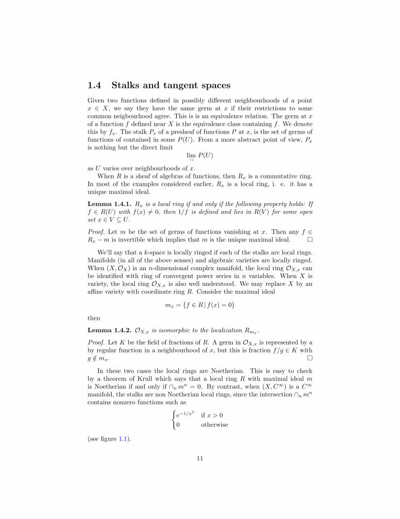
In these two cases the local rings are Noetherian. This is easy to checkby a theorem of Krull which says that a local ring R with maximal ideal mis Noetherian if and only if ∩n mn = 0. By contrast, when (X, C∞) is a C∞
manifold, the stalks are non Noetherian local rings, since the intersection ∩n mn
contains nonzero functions such ase−1/x2
if x > 00 otherwise
(see figure 1.1).
11
Figure 1.1: function in ∩n mn
However, the maximal ideals are finitely generated.
Proposition 1.4.3. If R is the ring of germs at 0 of C∞ functions on Rn.Then its maximal ideal m is generated by the coordinate functions x1, . . . xn.
If R is local ring with ring with maximal ideal m (which will denote by a pair(R,m)), then R/m is a field called the residue field. The cotangent space of Ris the R/m-vector space m/m2 ∼= m⊗R R/m, and the tangent space is its dual(over R/m). When m is finitely generated, these spaces are finite dimensional.When X is C∞ or complex manifold or an algebraic variety over k respectively,the local ring R = OX,x is an algebra over R, C or k and the map k → R→ R/mis an isomorphism. In these cases, we denote the tangent space - which is finitefdimensional - by TX,x or simply Tx. When R is the local ring of a manifold orvariety X at x, then R/m2 splits canonically into k ⊕ T ∗x . Given the germ of afunction f , let df be the projection to T ∗x . In other words, df = f − f(x).
Lemma 1.4.4. d : R→ T ∗x is a k-linear derivation, i. e. it satisfies the Leibnitzrule d(fg) = f(x)dg + g(x)df .
As a corollary, it follows that a tangent vector v ∈ Tx = T ∗∗x gives rise toa derivation v d : R → k. Conversely, any such derivation corresponds to atangent vector. In particular,
Lemma 1.4.5. If (R,m) is the ring of germs at 0 of C∞ functions on Rn.Then a basis for the tangent space T0 is given
Di =∂
∂xi
∣∣∣∣0
i = 1, . . . n
Exercise 1.4.6.
1. Prove proposition 1.4.3 (hint: given f ∈ m, let
fi =∫ 1
0
∂f
∂xi(tx1, . . . txn) dt
12
show that f =∑
fixi.)
2. Prove lemma 1.4.4.
3. Let F : (X, R) → (Y, S) be a morphism of k-spaces. If x ∈ X and y =F (x), check that the homorphism F ∗ : Sy → Rx taking a germ of f to thegerm of f F is well defined. When X and S are both locally ringed, showthat F ∗(my) ⊆ mx where m denotes the maximal ideals.
4. When F : X → Y is a C∞ map of manifolds, use the previous exerciseto construct the induced linear map dF : Tx → Ty. Calculate this for(X, x) = (Rn, 0) and (Y, y) = (Rm, 0) and convince yourself that thisreally is the derivative.
5. Check that with the appropriate identification given a C∞ function on Xviewed as a C∞ map from f : X → R. df in the sense of 1.4.4 and in thesense of the previous exercise coincide.
1.5 Nonsingular Varieties
Manifolds are locally quite simple. By contrast algebraic varieties can be locallyvery complicated. For example, any neighbourhood of the vertex of the coneover a projective variety is as complicated as the variety itself.
We want to say that a point of a variety is nonsingular if it looks like affinespace at a microscopic level. The precise definition requires some commutativealgebra:
Theorem 1.5.1. Let X ⊂ ANk be a closed subvariety defined by the ideal
(f1, . . . fr). Choose x ∈ X and let R = OX,x. Then the following statementsare equivalent
1. R is a regular local ring i.e. dim Tx equals the Krull dimension of R.
2. The rank of the Jacobian (∂fi/∂xj |x) is N − dim X.
3. The completion R is isomorphic to a ring of formal power series over k.
If these conditions are fulfilled, x is called a nonsingular point of X. Notethat the equivalence of (2) and (3) amounts to a formal implicit function theo-rem. When k = C, we can apply the holomorphic implicit function theorem todeduce an additional equivalent statement:
4 There exists a neighbourhood U of x ∈ CN in the usual Euclidean topology,and a biholomorphism (i. e. holomorphic isomorphism) of U to a ball Bsuch that X∩U maps to the intersection of B and an n-dimensional linearsubspace.
A variety is called nonsingular or smooth if all of its points are nonsingular.Affine and projective spaces are examples of nonsingular varieties. It followsfrom (4) that a nonsingular affine or projective variety is a complex submanifoldof affine or projective space.
13
1.6 Vector fields
A vector field on a manifold X is a choice vx ∈ Tx for each x ∈ X. Of course,we really want this function x→ vx to be C∞ in the appropriate sense. Thereare a few ways to make this precise. For the moment, we will rely on the crutchof coordinates. Choose an atlas
Fj : (Uj , C∞|Uj
) ∼= (Bj , C∞|Bj
)
then using the construction of the previous exercise, we can push the vectorfield onto the ball Bj . When we expand this in the basis
dFjvx =∑
fi(x)∂
∂xi
we require that the components are C∞ functions. The dual notion is that of1-form (or covector field). It is a choice of ωx ∈ T ∗x varying in a C∞ way. Thisdual notion is perhaps the more fundamental of the two. Given a Ci-functionf on X, we can define df = x 7→ dfx. This is a C∞ 1-form. This allows fora coordinate free formulation of the above notion. A vector field vx is C∞
exactly when the map x 7→ vx df ∈ C∞(X) for each f ∈ C∞(X).Let T (X) and E1(X) denote the space of C∞ vector fields on X. Then U 7→
T (U) and U 7→ E1(U) are easily seen to be sheaves on X denoted by TX and E1X
respectively. These are prototypes of sheaves of locally free C∞-modules: EachT (U) is a C∞(U)-module, and hence a C∞(V )-module for any U ⊂ V and therestriction T (V )→ T (U) is C∞(V )-linear. Every point has a neighbourhood Usuch that are T (U) and E1(U) are free C∞(U)-modules. More specifically, if U isa coordinate neighbourhood with coordinates x1, . . . xn, then ∂/∂x1, . . . ∂/∂xnand dx1, . . . dxn are bases for T (U) and E1(U) respectively.
These notions are usually phrased in the equivalent language of vector bun-dles. A rank n (C∞ real, holomorphic, algebraic) vector bundle is a morphismof C∞ or complex manifolds or algebraic varieties π : V → X such that thereexists an open cover Ui of X and commutatitve diagrams
φi : π−1Ui
∼=−→ Ui × kn
Ui
such that pi p−1j are linear on each fiber. Here k = R or C in the first two
cases. Given a vector bundle π : V → X, define the presheaf of sections
V (U) = s : U → π−1U | s is C∞, π s = idU
This is easily seen to be a sheaf of locally free modules. Conversely, we willsee in section 6.3 that every such sheaf arises this way. The vector bundlecorresponding to TX is called the tangent bundle of X.
Parallel constructions can be carried out for holomorphic (respectively reg-ular) vector fields and forms on complex manifolds and nonsingular algebraicvarieties. The corresponding sheaf of forms will be denoted by Ω1
X .
14
An explicit example of a nontrivial vector bundle is the tautological bundle.Projective space Pn
k is the set of lines through 0 in kn+1. Let
T = (x, l) ∈ kn+1 × Pnk |x ∈ l
Let P : T → Pnk be given by projection onto the second factor. Then T is rank
one algebraic vector bundle, or line bundle, over Pnk . When k = C this can also
be regarded as holomorphic line bundle.
Exercise 1.6.1.
1. Let S = Sn−1 ⊂ Rn denote the unit sphere. Let
TS = (v, w) ∈ Rn × S | v · w = 0
where · is the usual dot product. Check that the map TS → S given by thesecond projection makes, TS into a rank n − 1 vector bundle. This is anexplicit model for the tangent bundle of the sphere.
2. Check that T really is an algebraic line bundle.
15
Chapter 2
Generalities about Sheaves
Up to now, we have been dealing with sheaves primarily as a linguistic device; assets of functions with some properties. Here we want to do sheaf theory proper.
2.1 The Category of Sheaves
It will be convenient to define sheaves of things other than functions. Forinstance, one might consider sheaves of equivalence classes of functions. Forthis more general notion of presheaf, the restrictions maps have to be includedas part the data:
Definition 2.1.1. A presheaf P on a topological space X consists of a set P (U)for each open set U , and maps ρUV : P (U) → P (V ) for each inclusion V ⊂ Usuch that:
1. ρUU = idP (U)
2. ρV W ρUV = ρUW
We will usually write f |V = ρUV (f).
Definition 2.1.2. A presheaf P is a sheaf if for any open covering Ui of U ,given fi ∈ P (Ui) satisfying fi|Ui∩Uj = fj |Ui∩Uj , there exists a unique f ∈ P (U)with f |Ui
= fi.
Definition 2.1.3. A morphism of presheaves fU : P → P ′ is collection ofmaps fU : P (U)→ P ′(U) which commute with the restrictions. A morphism ofsheaves is defined exactly in the same way.
A special case of a morphism is the notion of a subsheaf of sheaf. Thisis a morphism of sheaves where each fU : P (U) ⊆ P ′(U) is an inclusion. Forexample, the sheaf of C∞-funtions on Rn is a subsheaf of the sheaf of continuousfunctions.
16
Example 2.1.4. Given a sheaf of rings of functions R over X, and f ∈ R(X),the map R(U)→ R(U) given multipication by f |U is a morphism.
Example 2.1.5. Let X be a C∞ manifold, then d : C∞ → E1 is a morphismof sheaves.
We now can define the category of presheaves of abelian groups PAb(X)on a topological space X, where we require the maps fU : P (U) → P ′(U) tobe homomorphisms. Let Ab(X) be the full subcategory of sheaves of abeliangroups on X. Let Ab denote the category of abelian groups. There are numberof functors from PAb(X) to Ab. The global section functor Γ(P ) = Γ(X, P ) =P (X). For any x ∈ X, define the stalk Px of the presheaf P at x, as the directlimit lim P (U) over neighbourhoods of x. Then P → Px determines a functorfrom PSh(X)→ Ab.
There is a functor going backwards from PAb(X)→ Ab(X) called sheafica-tion generalizating the previous construction.
Theorem 2.1.6. The sheafification functor P 7→ P+ has the following proper-ties:
1. There is a canonical morphism P → P+.
2. If P is a sheaf then this morphism is an isomomorphism
3. Any morphism from P to a sheaf factors uniquely through P → P+
4. The map P → P+ induces an isomorphism on stalks.
We sketch the construction under a mild (an unnecessary assumption) thatP (X) contains at least one element, which we will call 0. The construction willbe done in two steps. First, we construct presheaf of functions, then we previousconstruction to make this sheaf.
Set Y =∏
Px. We define a morphism from P to a sheaf P ′ of Y -valuedfunctions as follows. There is a canonical map σx : P (U)→ Px if x ∈ U ; if x /∈ Uthen send everything to 0. Then f ∈ P (U) defines a function f ′(x) = σx(f).Let P ′(U) be the set of f ′ with f ∈ P (U). Now we define P+ = (P ′)+.
2.2 Exact Sequences
We want to point out, for those who like this sort of thing, that the categoryAb(X) is an abelian category [GM, Wl] which means, roughly speaking, thatit possesses many of the basic constructions and properties of the category ofabelian groups. In particular, there is an intrinsic notion of an exactness in thiscategory. We give a nonintrinsic, but equivalent, formulation of this notion. Asequence of sheaves on X
A→ B → C
is called exact if and only if
Ax → Bx → Cx
17
is exact for every x ∈ X.
Lemma 2.2.1. Let f : A → B and g : B → C, then A → B → C is exact ifand only if for any open U ⊆ X
1. gU fU = 0.
2. Given b ∈ B(U) with g(b) = 0, there exists an open cover Ui of U andai ∈ A(Ui) such that f(ai) = b|Ui
.
Proof. We will prove one direction. Suppose that A→ B → C is exact. Givena ∈ A(U), g(f(a)) = 0, since g(f(a))x = g(f(ax)) = 0 for all x ∈ U .
For each x ∈ U , bx is the image of a germ in A at x. Choose a representativefor this germ in some A(Ux) where Ux is a neighbourhood of x.
Corollary 2.2.2. If A(U)→ B(U)→ C(U) is exact for every open set U , thenA→ B → C is exact.
The converse is false, but we do have:
Lemma 2.2.3. If0→ A→ B → C → 0
is an exact sequence of sheaves, then
0→ A(U)→ B(U)→ C(U)
is exact for every open set U .
Proof. Let f : A→ B and g : B → C denote the maps. By lemma 2.2.1,gf = 0.Suppose a ∈ A(U) maps to 0 under f , then f(ax) = f(a)x = 0 for each x ∈ U .Therefore ax = 0 for each x ∈ U , and this implies that a = 0.
Suppose b ∈ B(U) satisfies g(b) = 0. Then by lemma 2.2.1, there exists anopen cover Ui of U and ai ∈ A(Ui) such that f(ai) = b|Ui
. Then f(ai−aj) = 0,which implies ai − aj = 0 by the first part. Therefore ai − aj patch together toyield an element of A(U).
Example 2.2.4. Let X denote the circle S1 = R/Z. Then
0→ RX → C∞X
d−→ E1X → 0
is exact. However C∞(X)→ E1(X) is not surjective.
To see the first statement, let U ⊂ X be an open set diffeomorphic to anopen interval. Then the sequence
0→ R→ C∞(U)f→f ′−→ C∞(U)dx→ 0
is exact by calculus. Thus one gets exactness on stalks. For the second, notethat the constant form dx is not the differential of a periodic function.
18
Example 2.2.5. Let (X,OY ) be C∞ or complex manifold or algebraic varietyand Y ⊂ X a submanifold or subvariety. Let
IY (U) = f ∈ OX(U) | f |Y = 0
then0→ IY → OX → OY → 0
is exact. Example 1.2.10 shows that OX(X)→ OY (X) need not be surjective.
Given a sheaf S and a subsheaf S′ ⊆ S, we can define a new presheaf withQ(U) = S(U)/S′(U) and restriction maps induced from S. In general, this isnot a sheaf.
Exercise 2.2.6.
1. Finish the proof of lemma 2.2.1.
2. Give an example of a subsheaf S′ ⊆ S, where Q(U) = S(U)/S′(U) fails tobe a sheaf. Check that
0→ S′ → S → S/S′ → 0
is an exact sequence of sheaves.
3. Given a morphism of sheaves f : S → S′, define ker f to be the subpresheafof S with ker f(U) = ker[fU : S(U)→ S′(U)]. Check that ker f is a sheaf,and check that (ker f)x
∼= ker[Sx → S′x].
2.3 The notion of a scheme
A scheme is a massive generalization of the notion of an algebraic variety due toGrothendieck. We will give only the basic flavour of the subject. The canonicalreference is [EGA]. Hartshorne’s book [H] has become the standard introductionto these ideas for a more most people.
Let R be a commutative ring. Let SpecR denote the set of prime ideals ofR. For any ideal, I ⊂ R, let
V (I) = p ∈ SpecR | I ⊆ p.
Lemma 2.3.1. 1. V (IJ) = V (I) ∪ V (J).
2. V (∑
Ii) = ∩i V (Ii),
As a corollary, it follows that the sets of the form V (I) form the closedsets of a topology on Spec R called the Zariski topology. Note that when R isthe coordinate ring of an affine variety Y over an algebraically closed field k.The Hilbert Nullstellensatz shows that any maximal ideal of R is of the formmy = f ∈ R | f(y) = 0 for a unique y ∈ Y . Thus we can embed Y into Spec R
19
by sending y to my. Under this embedding V (I) pulls back to the algebraicsubset
y ∈ Y | f(y) = 0, ∀f ∈ I
Thus this notion of Zariski topologu is an extension of the classical one.A basis is the Zariski topology on X = Spec R is given by D(f) = X−V (f).
Thus any open set U ⊂ X is a union of such sets. Define
OX(U) = lim→
R[1f
]
When R is an integral domain with fraction field K, OX(U) ⊂ K consists of theelements r such that for any p ∈ U , r = g/f with f /∈ p. This remark applies,in particular, to the case where R is the coordinate ring of an algebraic varietyY . In this case, OX(U) can be identified with the ring of regular functions onU ∩ Y under the above embedding.
Lemma 2.3.2. OX is a sheaf of commutative rings such that OX,p∼= Rp for
any p ∈ X.
Proof. We give the proof in the special case where R is a domain. This impliesthat X is irreducible, i. e. any two nonempty open sets intersect, because
D(gi) ∩D(gj) = D(gigj) 6= ∅
if gi 6= 0. Consequently the constant presheaf KX with values in K is already asheaf. OX is a subpresheaf of KX . Let U = ∪Ui be a union of nonempty opensets, and fi ∈ OX(Ui). Then fi = fj as elements of K. Call the common valuef . Since p ∈ U lies in some Ui, f can be written as a fraction with denominatorin R− p. Thus f ∈ OX(U), and this shows that OX is a sheaf.
One sees readily that the stalk OX,p is the subring of K of fractions wherethe denominator can be chosen in R− p. Thus OX,p
∼= Rp.
The pair (X,OX) is called the affine scheme associated to R. A schemeconsists of a topological space together with a sheaf of rings which is locallyisomorphic to an affine scheme. We have seen how to associate an affine schemeto an affine variety. More generally, given a (pre)variety Y over a field k, thereexists a scheme X and embedding Y → X such that OX restricts to the sheafof regular functions on Y . In particular, all the information about Y can berecovered from X. At this point, one can redefine the varieties as special kindsof schemes. We will take up these ideas again in section 16.1.
2.4 Toric Varieties
Toric varieties are an interesting class of varieties that are explicitly constructedby gluing of affine schemes. The beauty of the subject stems from the inter-play between the algebraic geometry and the combinatorics. See [F] for furtherinformation (including an explanation of the name).
20
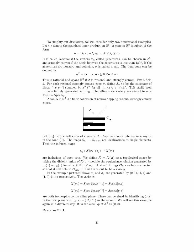
To simplify our discussion, we will consider only two dimensional examples.Let 〈, 〉 denote the standard inner product on R2. A cone in R2 is subset of theform
σ = t1v1 + t2v2 | ti ∈ R, ti ≥ 0
It is called rational if the vectors vi, called generators, can be chosen in Z2,and strongly convex if the angle between the generators is less than 180o. If thegenerators are nonzero and coincide, σ is called a ray. The dual cone can bedefined by
σ∨ = v | 〈v,w〉 ≥ 0,∀w ∈ σ
This is rational and spans R2 if σ is rational and strongly convex. Fix a fieldk. For each rational strongly convex cone σ, define Sσ to be the subspace ofk[x, x−1, y, y−1] spanned by xmyn for all (m,n) ∈ σ∨ ∩ Z2. This easily seento be a finitely generated subring. The affine toric variety associated to σ isX(σ) = Spec Sσ.
A fan ∆ in R2 is a finite collection of nonoverlapping rational strongly convexcones.
σ
σ1
2
Let σi be the collection of cones of ∆. Any two cones interest in a ray orin the cone 0. The maps Sσi
→ Sσi∩σjare localizations at single elements.
Thus the induced maps
ιij : X(σi ∩ σj)→ X(σi)
are inclusions of open sets. We define X = X(∆) as a topological space bytaking the disjoint union of X(σi) modulo the equivalence relation generated byιij(x) ∼ ιji(x) for all x ∈ X(σi ∩ σj). A sheaf of rings OX can be constructedso that it restricts to OX(σi). This turns out to be a variety.
In the example pictured above σ1 and σ2 are generated by (0, 1), (1, 1) and(1, 0), (1, 1) respectively. The varieties
X(σ1) = Spec k[x, x−1y] = Spec k[x, t]
X(σ2) = Spec k[y, xy−1] = Spec k[y, s]
are both isomorphic to the affine plane. These can be glued by identifying (x, t)in the first plane with (y, s) = (xt, t−1) in the second. We will see this exampleagain in a different way. It is the blow up of A2 at (0, 0).
Exercise 2.4.1.
21
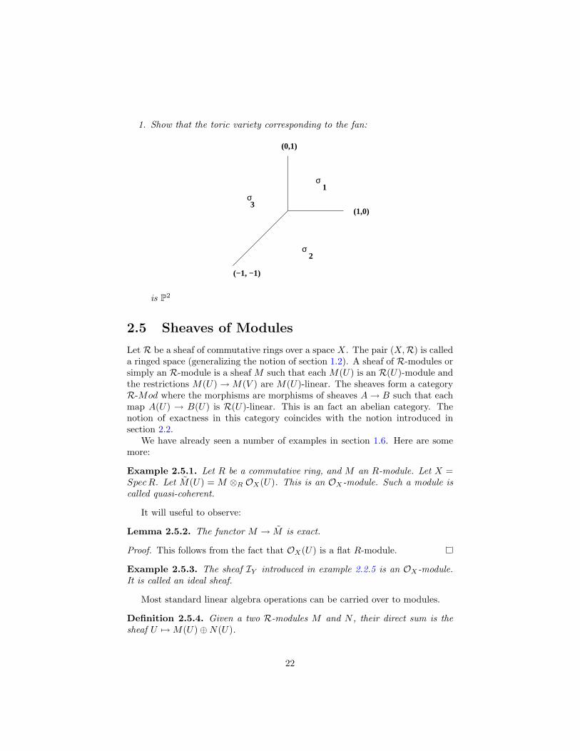
1. Show that the toric variety corresponding to the fan:
(1,0)
(0,1)
(−1, −1)
σ
σ
σ
1
2
3
is P2
2.5 Sheaves of Modules
Let R be a sheaf of commutative rings over a space X. The pair (X,R) is calleda ringed space (generalizing the notion of section 1.2). A sheaf of R-modules orsimply an R-module is a sheaf M such that each M(U) is an R(U)-module andthe restrictions M(U)→M(V ) are M(U)-linear. The sheaves form a categoryR-Mod where the morphisms are morphisms of sheaves A→ B such that eachmap A(U) → B(U) is R(U)-linear. This is an fact an abelian category. Thenotion of exactness in this category coincides with the notion introduced insection 2.2.
We have already seen a number of examples in section 1.6. Here are somemore:
Example 2.5.1. Let R be a commutative ring, and M an R-module. Let X =SpecR. Let M(U) = M ⊗R OX(U). This is an OX-module. Such a module iscalled quasi-coherent.
It will useful to observe:
Lemma 2.5.2. The functor M → M is exact.
Proof. This follows from the fact that OX(U) is a flat R-module.
Example 2.5.3. The sheaf IY introduced in example 2.2.5 is an OX-module.It is called an ideal sheaf.
Most standard linear algebra operations can be carried over to modules.
Definition 2.5.4. Given a two R-modules M and N , their direct sum is thesheaf U 7→M(U)⊕N(U).
22
Definition 2.5.5. The dual M∗ of a R-module M is the sheaf associated toU 7→ HomR(U)(M(U),R(U)).
For example the sheaf of 1-forms on a manifold is the dual of the tangentsheaf.
Definition 2.5.6. Given two R-modules M and N , their tensor product is thesheaf associated to U 7→M(U)⊗R(U) N(U).
Given a module M over a commutative ring R, recall that the exterior al-gebra ∧∗M (respectively symmetric algebra S∗M) is the quotient of the freeassociative algebra with multiplication ∧ (resp. ·) by the two sided ideal gen-erated m ∧ m (resp. (m1 · m2 − m2 · m1)). ∧kM (SkM) is the submodulegenerated by products of k elements. If V is a finite dimensional vector space,∧kV ∗ (SkV ∗) can be identified with the set of alternating (symmetric) multilin-ear forms on V in k-variables. After choosing a basis for V , one sees that SkV ∗
are degree k polynomials in the coordinates.
Definition 2.5.7. When M is an R-module, the kth exterior power ∧kM issheaf associated to U 7→ ∧kM(U) When X is manifold the sheaf of k-forms isEk
X = ∧kE1X .
Definition 2.5.8. A module M is locally free (of rank n) if for every point hasa neighbourhood U , such that M |U is isomorphic to a finite (n-fold) direct sumR|U ⊕ . . .⊕R|U
Given an R-module M over X, the stalk Mx is an Rx-module for any x ∈ X.If M is locally free, then each stalk is free of finite rank. Note that the conversemay fail.
As noted in section 1.6, locally free sheaves arise from vector bundles. Let Tbe the tautological line bundle on projective space P = Pn
k over an algebraicallyclosed field k. The sheaf of regular sections is denoted by OP(−1) = OPn
k(−1).
OP(1) is the dual and
OP(m) =
SmO(1) = O(1)⊗ . . . O(1) (m times) if m > 0OP if m = 0S−mO(−1) = O(−m)∗ otherwise
Let V = kn+1. By construction T ⊂ V × Pn, so OP(−1) is a subsheaf of then+1-fold sum OP⊕. . .⊕OP which can be expressed more canonically as V ⊗kOP.Dualizing, gives
V ∗ ⊗OP → OP(1)→ 0
Taking symmetric powers gives a map, in fact an epimorphism
SmV ∗ ⊗OP → OP(m)→ 0
when m ≥ 0. Taking global sections gives maps
SmV ∗ → SmV ∗ ⊗ Γ(OP)→ Γ(OP(m))
23

We will see later that these maps are isomorphisms. Thus the global sections ofOP(m) are homogenous degree m polynomials in the homogeneous coordinatesof m.
Exercise 2.5.9.
1. Show that the stalk of M at p is precisely the localization Mp.
2. Show that direct sums, tensor products, exterior, and symmetric powersof locally free sheaves are locally free.
2.6 Direct and Inverse images
Given any subset S ⊂ X of a topological space and a presheaf F , define
F(S) = lim→F(U)
as U ranges over all open neigbourhoods of S. If S is point, this is just thestalk.
Let F : X → Y be a continous map of topological spaces. Given a sheaf Aon X, define the the direct image sheaf F∗A on Y by F∗A(U) = A(F−1U) withobvious restrictions. If B is a sheaf on Y , define F−1B(V ) = B(F (V )). (Thelack of symmetry in the notation will be fixed in a moment.) These operationsare clearly functors f∗ : Ab(X) → Ab(Y ) and f−1 : Ab(Y ) → Ab(X). Therelationship is given by the adjointness property:
Lemma 2.6.1. There is a natural isomorphism
HomAb(X)(f−1A,B) ∼= HomAb(Y )(A, f∗B)
Given a morphism F of k-spaces (X,R) → (Y,S) (section 1.2), we get amorphism of sheaves rings S → F∗R given by f 7→ f F . More generally,we can define a morphism of ringed spaces to be a continuous map togethera morphism of rings S → F∗R. Let f−1S → R be the adjoint map. Givenan R-module M , f∗M is naturally an f∗R-module, and hence an S-module byrestriction of scalars. Similarly given an S-module N , f−1N is naturally anf−1S-module. We define the R-module
f∗N = R⊗f−1S f−1N
The inverse image of a locally sheaf is locally free. This has an an interpre-tation in the context of vector bundles 1.6. If π : V → Y is a vector bundle,then the vector bundle f∗V → X can be defined in the context of manifolds orvarieties. Set theoretically, it is the projection
f∗V = (v, x) |π(v) = f(x) → X
Thenf∗(sheaf of sections of V ) = (sheaf of sections of f∗V )
24
Exercise 2.6.2.
1. Check that f∗A and f−1B are really sheaves.
2. Prove lemma 2.6.1.
3. Generalize lemma 2.2.3 to show that an exact sequence 0 → A → B →C → 0 of sheaves gives rise to an exact sequence 0→ f∗A→ f∗B → f∗C.
25

Chapter 3
Sheaf Cohomology
In this chapter, we give a rapid introduction to sheaf cohomology. It lies at theheart of everything else in these notes.
3.1 Flabby Sheaves
A sheaf F on X is called flabby (or flasque) if the restriction maps F(X)→ F(U)are surjective for any nonempty open set. Their importance stems from thefollowing:
Lemma 3.1.1. If 0 → A → B → C is an exact sequence of sheaves with Aflabby, then B(X)→ C(X) is surjective.
Proof. We will prove this by the no longer fashionable method of transfiniteinduction1. Let γ ∈ C(X). By assumption, there is an open cover Uii∈I ,such that γ|Ui lifts to a section βi ∈ B(Ui). By the well ordering theorem, wecan assume that the index set I is the set of ordinal numbers less than a givenordinal κ. We will define
σi ∈ B(∪j<iUj)
inductively, so that it maps to the restriction of γ. Set σ1 = β0. If σi exists, letαi be an extension of βi − σi to A(X). Then set σi+1 to be σi on the Uj , j < i,and βi − αi|Ui
on Ui. If i is a limit (non-successor) ordinal, then the previousσ’s patch to define σi. Then σκ is a global section of B mapping to γ.
Corollary 3.1.2. The sequence 0 → A(X) → B(X) → C(X) → 0 is exact ifA is flabby.
Example 3.1.3. Let X be a space with the property that any open set is con-nected (e.g. X is irreducible). Then any constant sheaf is flabby.
1For most cases of interest to us, X will have a countable basis, so ordinary induction willsuffice
26
Let F be a presheaf, define the presheaf G(F) by
U 7→∏x∈U
Fx
with the obvious restrictions. There is a canonical morphism F → G(F).
Lemma 3.1.4. G(F) is a flabby sheaf, and the morphism is F → G(F) is amonomorphism if F is a sheaf.
Lemma 3.1.5. G and Γ G are exact functors on the category of sheaves i. e.they preserves exactness.
Exercise 3.1.6.
1. Find a proof of lemma 3.1.1 which uses Zorn’s lemma.
2. Prove that the sheaf of bounded continous real valued functions on R isflabby
3. Prove the same thing for the sheaf of bounded C∞ functions on R.
4. Prove that if 0→ A→ B → C is exact and A is flabby, then 0→ f∗A→f∗B → f∗C → 0 is exact for any continuous map f .
3.2 Cohomology
Define C0(F) = F , C1(F) = coker[F → G(F)] and Cn+1(F) = C1Cn(F).Now cohomology can be defined by:
H0(X,F) = Γ(X,F)H1(X,F) = coker[Γ(X, G(F))→ Γ(X, C1(F))]
Hn+1(X,F) = H1(X, Cn(F))
Hi(X,−) is clearly a functor from Ab(X)→ Ab. Another basic property isthe following which says in effect that these form a “delta functor” [Gr, H].
Theorem 3.2.1. Given an exact sequence of sheaves
0→ A→ B → C → 0,
there is a long exact sequence
0→ H0(X, A)→ H0(X, B)→ H0(X, C)→
H1(X, A)→ H1(X, B)→ H1(X, C)→ . . .
First we need:
27

Lemma 3.2.2. There is a commutative diagram with exact rows
0 0 0↓ ↓ ↓
0 → A → B → C → 0↓ ↓ ↓
0 → G(A) → G(B) → G(C) → 0↓ ↓ ↓
0 → C1(A) → C1(B) → C1(C)
Proof. By lemma 3.1.5, there is a commutative diagram with exact rows
0 0 0↓ ↓ ↓
0 → A → B → C → 0↓ ↓ ↓
0 → G(A) → G(B) → G(C) → 0
The snake lemma [AM, GM] (which holds in any abelian category) gives therest.
Proof. From the previous lemma and lemmas 2.2.3 and 3.1.5, we get a commu-tative diagram with exact rows:
0 → Γ(G(A)) → Γ(G(B)) → Γ(G(C)) → 0↓ ↓ ↓
0 → Γ(C1(A)) → Γ(C1(B)) → Γ(C1(C))
From the snake lemma, we obtain a 6 term exact sequence
0→ H0(X, A)→ H0(X, B)→ H0(X, C)
→ H1(X, A)→ H1(X, B)→ H1(X, C)
Repeating this with A replaced by C1(A), C2(A) . . . allows us to continue thissequence indefinitely.
Corollary 3.2.3. B(X)→ C(X) is surjective if H1(X, A) = 0.
Exercise 3.2.4.
1. If F is flabby prove that Hi(X,F) = 0 for i > 0. (Prove this for i = 1,and that F flabby implies that C1(F) is flabby.)
3.3 Soft sheaves
Up to now, the discussion has been abstract. In this section, we will actuallydo some computations. We first need to introduce a class of sheaves which aresimilar to flabby sheaves, but much more plentiful. We assume through out thissection that X is a metric space although the results hold under the weakerassumption of paracompactness.
28
Definition 3.3.1. A sheaf F is called soft if the map F(X)→ F(S) is surjectivefor all closed sets.
Lemma 3.3.2. If 0 → A → B → C is an exact sequence of sheaves with Asoft, then B(X)→ C(X) is surjective.
Proof. The proof is very similar to the proof of 3.1.1. We just indicate themodifications. We can assume that the open cover Ui consists of open balls.Let Vi be a new open cover where we shrink the radii of each ball, so thatVi ⊂ Ui. Define
σi ∈ B(∪j<iVj)
inductively as before.
Corollary 3.3.3. If A and B are soft then so is C.
One trivially has:
Lemma 3.3.4. A flabby sheaf is soft.
Lemma 3.3.5. If F is soft then Hi(X,F) = 0 for i > 0.
Proof. Lemma 3.3.2 H1(F) = 0. Lemma 3.3.4 implies that Ci(F) is soft, henceHi(F) = 0.
Theorem 3.3.6. The sheaf CR of continuous real valued functions on a metricspace X is soft.
Proof. Suppose S is closed subset and f : U → R a real valued continuousfunction defined in a neighbourhood of S. We have to extend the germ of f toX. Let d denote the metric. We extend this to a fuction d(A,B) on pairs ofsubsets A,B ⊆ X by taking the inf over all d(a, b) with a ∈ A and b ∈ B. LetS′ = X − U and let
g(x) =
d(x, S′)/ε if d(x, S′) < ε1 otherwise
where ε = d(S, S′)/2. Then gf extends by 0 to a continous function on X.
Note that CR is almost never flabby. We get many more examples of softsheaves with the following.
Lemma 3.3.7. Let R be a soft sheaf of rings, then any R-module is soft.
Proof. The basic strategy is the same as above. Let f be section of anR-moduledefine in the neighbourhood of a closed set S, and let S′ be the complementof this neighbourhood . Since R is soft, the section which is 1 on S and 0 onS′ extends to a global section g. Then gf extends to a global section of themodule.
U ⊂ C denote the unit circle, and let e : R → U denote the normalizedexponential e(x) = exp(2πix). Let us say that X is locally simply connected ifevery neighbourhood of every point contains a simply connected neighbourhood.
29
Lemma 3.3.8. If X is locally simply connected, then the sequence
0→ ZX → CRe−→ CU → 1
is exact.
Lemma 3.3.9. If X is simply connected and locally simply connected, thenH1(X, ZX) = 0.
Proof. Since X is simply connected, any continuous map from X to U can belifted to a continuous map to its universal cover R. In other words, CR(X)surjects onto CU (X). Since CR is soft, lemma 3.3.8 implies that H1(X, ZX) =0.
Corollary 3.3.10. H1(Rn, Z) = 0.
Exercise 3.3.11.
1. Check that the sheaf C∞ functions on Rn is soft.
3.4 Mayer-Vietoris sequence
We will introduce a basic tool for computing cohomology groups which is preludeto Cech cohomology. Let U ⊂ X be open. For any sheaf, we want to definenatural restriction maps Hi(X,F) → Hi(U,F). If i = 0, this is just the usualrestriction. For i = 1, we have a commutative square
Γ(X, G(F)) → Γ(X, C1(F))↓ ↓
Γ(U,G(F)) → Γ(U,C1(F))
which induces a map on the cokernels. In general, we use induction.
Theorem 3.4.1. Let X be a union to two open sets U ∪ V , then for any sheafthere is a long exact sequence
. . .Hi(X,F)→ Hi(U,F)⊕Hj(V,F)→ Hi(U ∩ V,F)→ Hi+1(X,F) . . .
where the first indicated arrow is the sum of the restrictions, and the second isthe difference.
Proof. The proof is very similar to the proof of theorem 3.2.1, so we will justsketch it. Construct a diagram
0 → Γ(X, G(F)) → Γ(U,G(F))⊕ Γ(V,G(F)) → Γ(U ∩ V,G(F)) → 0↓ ↓ ↓
0 → Γ(X, C1(F)) → Γ(U,C1(F))⊕ Γ(V,C1(F)) → Γ(U ∩ V,C1(F))
and apply the snake lemma to get the sequence of the first 6 terms. Then repeatwith Ci(F) in place of F .
30
Exercise 3.4.2.
1. Use Mayer-Vietoris to prove that H1(S1, Z) ∼= Z.
2. Show that H1(Sn, Z) = 0 if n ≥ 2.
31

Chapter 4
De Rham’s theorem
In this chapter, we apply the machinery of the last section to the study of C∞
manifolds.
4.1 Acyclic Resolutions
A complex of abelian groups (or more generally elements in an abelian category)is a possibly infinite sequence
. . . F i di
−→ F i+1 di+1
−→ . . .
of groups an homomorphisms satisfying di+1di = 0. These condtions guaranteethat image(di) ⊆ ker(di+1). We denote a complex by F • and we often suppressthe indices on d. The cohomology groups of F • are defined by
Hi(F •) ∼=ker(di+1)image(di)
For example, an exact sequence is a complex where the groups are zero.The connection, between this notion of cohomology and the previous one
will be established shortly. A sheaf F is called acyclic if Hi(X,F) = 0 for alli > 0. An acyclic resolution of F is a exact sequence
0→ F → F0→F1→ . . .
of sheaves such that each F i is acyclic. Given the a complex, the sequence
Γ(X,F0)→ Γ(X,F1)→ . . .
need not be exact, however it is necessarily a complex by functoriallity.
Theorem 4.1.1. Given an acyclic resolution of F as above,
Hi(X,F) ∼= Hi(Γ(X,F•))
32
Proof. Let K−1 = F and Ki = ker(F i+1 → F i+2). Then there are exactsequences
0→ Ki−1 → F i → Ki → 0
Since F i are acyclic, theorem 3.2.1 implies that
0→ H0(Ki−1)→ H0(F i)→ H0(Ki)→ H1(Ki−1)→ 0 (4.1)
is exact, andHj(Ki) ∼= Hj+1(Ki−1) (4.2)
for j > 0. The sequences (4.1) leads to a commutative diagram
H0(Ki−1) //___ H0(F i) //
%%JJJJJJJJJH0(F i+1)
H0(Ki)
99rr
rr
r
where the dashed arrows are injective. Therefore
H0(Ki−1) ∼= ker[H0(F i)→ H0(F i+1)]
This already implies the first case of the theorem when i = 0. This isomorphismtogether with the sequence (4.1) implies that
H1(Ki−1) ∼=ker[H0(F i+1)→ H0(F i+2)]
image[H0(F i)]
Combining this with the isomorphisms
Hi+1(K−1) ∼= Hi(K0) ∼= . . .H1(Ki−1)
of with (4.2) finishes the proof.
4.2 De Rham’s theorem
Let X be a C∞ manifold and Ek = EkX the sheaf of k-forms. Note that E0 = C∞.
Theorem 4.2.1. There exists canonical maps d : Ek(X) → Ek+1(X), calledexterior derivatives, satisfying the following
1. d : E0(X)→ E1(X) is the operation introduced in section 1.6.
2. d2 = 0.
3. d(α ∧ β) = dα ∧ β + (−1)iα ∧ dβ for all α ∈ E i(X), β ∈ Ej(X).
33
Proof. A complete proof can be found in almost any book on manifolds (e.g.[Wa]). We will only sketch the idea. When X is a ball in Rn with coordinatesxi, one sees that there is a unique operation satisfying the above rules given by
d(fdxi1 ∧ . . . ∧ dxik) =
∑j
∂f
∂xjdxj ∧ dxi1 ∧ . . . dxik
This applies to any coordinate chart. By uniqueness, these local d’s patch.
When X = R3, d can be realized as the div, grad, curl of vector calculus. Thetheorem tells that E•(X) forms a complex. We define the De Rham cohomologygroups (actually vector spaces) as
HkdR(X) = Hk(E•(X))
Notice that the exterior derivative is really a map of sheaves d : EkX → E
k+1X
satisfying d2 = 0. Thus we have complex. Moreover, RX is precisely the kernelof d : E0
X → E1X .
Theorem 4.2.2. The sequence
0→ RX → E0X → E1
X . . .
is an acyclic resolution of RX .
Corollary 4.2.3 (De Rham’s theorem).
HkdR(X) ∼= Hk(X, R)
The theorem makes two seperate assertions, first that the complex is exact,then that the sheaves Ek are acyclic. The exactness follows from:
Theorem 4.2.4 (Poincare’s lemma). For all n and k > 0,
Hk(Rn) = 0.
Proof. Assume, by induction, that the theorem holds for n − 1. Identify Rn−1
the hyperplane x1 = 0. Let I be the identity and R : Ek(Rn) → Ek(Rn) berestriction to this hyperplane. Note that R commute with d. So if α ∈ Ek(Rn)is closed which means that dα = 0. Then dRα = Rdα = 0. By the inductionassumption, Rα is exact which means that it lies in the image of d.
For each k, define a map h : Ek(Rn)→ Ek−1(Rn) by
h(f(x1, . . . xn)dx1 ∧ dxi2 ∧ . . .) = (∫ x1
0
fdx1)dxi2 ∧ . . .
andh(fdxi1 ∧ dxi2 ∧ . . .) = 0
if 1 /∈ i1, i2, . . .. Then one checks that dh + hd = I − R (in other words,h is homotopy from I to R). Given α ∈ Ek(Rn) satisfying dα = 0. We haveα = dhα + Rα. Which by the above remarks is exact.
34
Corollary 4.2.5. The sequence of theorem 4.2.2 is exact.
Proof. Any ball is diffeomorphic to Euclidean space, and any point on a manifoldhas a fundamental system of such neigbourhoods. There the sequence is exacton stalks.
To prove that the sheaves Ek are acyclic, it’s enough to establish the follow-ing.
Lemma 4.2.6. E0 is soft.
In later, we will work with complex valued differential forms. Essentially thesame argument shows that H∗(X, C) can be computed using such forms.
Exercise 4.2.7.
1. We will say that a manifold is of finite type if it has a finite open coverUi such that any nonempty intersection of the Ui are diffeomorphic tothe ball. Compact manifolds are known to have finite type [Spv, pp 595-596]. Using Mayer-Vietoris and De Rham’s theorem, prove that if X is ann-dimensional manifold of finite type, then Hk(X, R) vanishes for k > n,and is finite dimensional otherwise.
4.3 Poincare duality
Let X be an C∞ manifold. Let Ekc (X) denote the set of C∞ k-forms with
compact support. Since dEkc (X) ⊂ Ek+1
c (X), we can define compactly supportedde Rham cohomology by
HkcdR(X) = Hk(E•c (X)).
Lemma 4.3.1. For all n,
HkcdR(Rn) =
R if k = n0 otherwise
The computation for Euclidean space suggests that these groups are someopposite to the usual ones. The precise statement, in general, requires thenotion of orientation. An orientation on an n dimensional real vector spaceV is a connected component of ∧nV − 0. This component serves to tellswhen an ordered basis v1, . . . vn is positively oriented; it is if v1 ∧ . . . vn lies inthis component. An orientation on an n dimensional manifold X is a choice ofconnected of ∧nTX minus the zero section.
Theorem 4.3.2. Let X be an oriented n-dimensional manifold. Then
HkcdR(X) ∼= Hn−k(X, R)∗
35
With the same notation as above, let Ck(U) = En−kc (U)∗ for any open set
U ⊂ X. Given V ⊂ U , α ∈ Ck(U), β ∈ Ek(V ), let α|V (β) = α(β) where β isthe extension of β by 0. This makes Ck a presheaf.
Lemma 4.3.3. Ck is a sheaf.
Proof. Let Ui be an open cover of U , and αi ∈ Ck(Ui). Let ρi be a C∞
partition of unity subordinate to Ui. Then define α ∈ Ck(U) by
α(β) =∑
i
αi(ρiβ)
Suppose that β ∈ Ekc (Uj) is extended by 0 to U . Then ρiβ will be supported in
Ui ∩ Uj . Consequently, αi(ρiβ) = αj(ρiβ). Therefore
α(β) = αj(∑
i
ρiβ) = αj(β).
Define a map δ : Ck(U)→ Ck+1(U) by δ(α)(β) = α(dβ). One automaticallyhas δ2 = 0. Thus one has a complex of sheaves.
The final ingredient is existence of the integral.
Theorem 4.3.4. Let X be an oriented n-dimensional manifold. There exists alinear map
∫X
: Enc (X)→ R such that
∫X
dβ = 0.
The details can be found in several places such as [Wa]. The last statementis a special case of Stoke’s theorem on a manifold. In essence, the construc-tion is similar to the proof of the previous lemma. Using a partition of unitysubordinate to an atlas one expresses∫
X
β =∫
X
(∑
i
ρiβ)
The right hand itegrals can be expressed in local coordinates in Euclidean space.The orientation is necessary in order to guarantee that these Euclidean integralsare chosen with a consistent sign.
We define a map RX → C0 induced by the map from the constant presheafsending r → r
∫X
. Then theorem 4.3.2 follows from
Lemma 4.3.5.0→ RX → C0 → C1 → . . .
is an acyclic resolution.
Proof. Lemma 4.3.1 implies that this complex is exact. The sheaves Ck are softsince they are C∞-modules.
36
We can now use this complex to compute the cohomology of RX to get
Hi(X, R) ∼= Hi(C•(X)) = Hi(E•c (X)∗)
and one sees more or less immediately that the right hand space is isomorphicto Hi
cdR(X, R)∗. This completes the proof of the theorem.
Corollary 4.3.6. If X is a compact oriented n-dimensional manifold. Then
Hk(X, R) ∼= Hn−k(X, R)∗
The following is really a corollary of the proof.
Corollary 4.3.7. If X is a connected oriented n-dimensional manifold. Thenthe map α 7→
∫X
α induces an isomorphism (denoted by same symbol)∫X
: HncdR(X, R) ∼= R
From now on, let us suppose that X is compact connected oriented n di-mensional manifold. We can make the duality isomorphism much more explicit.The de Rham cohomology is a graded ring with multplication denoted by ∪. Ifα and β are closed (i. e. lie in the kernel of d), then so is α∧β by theorem 4.2.1.If [α] and [β] denote the classes in H∗
dR(X) represented by these forms, thendefine [α]∪ [β] = [α∧ β]; this is well defined. The following will be proved lateron (cor. 7.2.2):
If f ∈ Hn−i(X, R)∗, then there exists a unique α ∈ Hi(X, R) such thatf(β) =
∫X
α ∪ β.
4.4 Fundamental class
Let Y ⊂ X be a closed connected oriented m dimensional manifold. Denote theinclusion by i. There is a natural restriction map
i∗ : Ha(X, R)→ Ha(Y, R)
induced by restriction of forms. Using Poincare duality we get a map going inthe opposite direction
i! : Ha(Y, R)→ Ha+n−m(X, R)
called the Gysin map. We want to make this more explicit. But first, we need:
Theorem 4.4.1. There exists an open neigbourhood T , called a tubular neig-bourhood, of Y in X and a π : T → Y which makes T a locally trivial rank(n−m) real vector bundle over Y .
Proof. See [Spv, p. 465].
37

We can factor i! as a composition
Ha(Y )→ Ha+n−mcdR (T )→ Ha+n−m(X)
where the first map is the Gysin map for the inclusion Y ⊂ T and the second isextension by zero. The first map is an isomorphism since it is dual to
Hm−a(T )∼=→ Hm−a
cdR (Y )
Let 1Y denote constant function 1 on Y . This is the natural generator forH0(Y, R). The Thom class τY of T is the image of 1Y under the isomorphismH0(Y )→ Hn−m
cdR (T ). τY can be reprsented by any closed compactly supportedn −m form on T whose integral along any fiber is 1. It is possible to choosea neighbourhood U of a point of Y with local coordinates xi, such that Y isgiven by xm+1 = . . . xn = 0 and π is given by (x1, . . . xn) 7→ (x1, . . . xm). Therestriction map
HicdR(T )→ Hi−n−m(U)⊗Hn−m
cdR (Rn−m)
is an isomorphism. Therefore the Thom class can be represented by an expres-sion
f(xm+1, . . . xn)dxm+1 ∧ . . . dxn
where f is compactly supported in Rn−m.The image of τY in Hn−m(X, R) is called the fundamental class [Y ] of Y .
The basic relation is given by∫Y
i∗α =∫
X
[Y ] ∪ α (4.3)
Let Y, Z ⊂ X be oriented submanifolds such that dimY + dimZ = n. Then[Y ]∪ [Z] ∈ Hn(X, R) ∼= R corresponds to a number Y ·Z. This has a geometricinterpretation. We say that Y and Z are transverse if Y ∩ Z is finite andif TY,p ⊕ TZ,p = TX,p for each p in the intersection. Choose ordered basesv1(p), . . . vm(p) ∈ TY,p and vm+1(p) . . . vn(p) ∈ TZ,p which are positively orientedwith respect to the orientations of Y and Z. We define the intersection number
ip(Y, Z) =
+1 if v1(p) . . . vn(p) is positively oriented−1 otherwise
This is easily seen to be independent of the choice of bases.
Proposition 4.4.2. Y · Z =∑
p ip(Y, Z)
Proof. Choose tubular neighbourhoods T of Y and T ′ of Z. These can be chosen“small enough” so that T ∩ T ′ is a union of disjoint neighbourhoods around Up
each p ∈ Y ∩ Z diffeomorphic to Rn = Rdim Y × Rdim Z Then
Y · Z =∫
X
τY ∧ τZ =∑
p
∫Up
τY ∧ τZ
38
Choose coordinates x1, . . . xn around p so that Y is given by xm+1 = . . . xn = 0and Z by x1 = . . . xm = 0. Then as above, the Thom classes of T and T ′ canbe written as
τY = f(xm+1, . . . xn)dxm+1 ∧ . . . dxn
τZ = g(x1, . . . xm)dx1 ∧ . . . dxm
Fubini’s theorem gives ∫Up
τY ∧ τZ = ip(Y, Z)
4.5 Examples
We look as some basic examples to illustrate the previous ideas. Let T = Rn/Zn.Let ei be the standard basis, and xi be coordinates on Rn. Then
Proposition 4.5.1. Every de Rham cohomology class on T contains a uniqueform with constant coefficients.
We will postpone the proof until section 7.2.
Corollary 4.5.2. There is an algebra isomorphism H∗(T, R) ∼= ∧∗Rn
Since T is a product of circles, this also follows from repeated application ofthe Kunneth formula:
Theorem 4.5.3. Let X and Y be C∞ manifolds, and let p : X × Y → X andq : X × Y → Y be the the projections. Then the map∑
αi ⊗ βj 7→∑
αi ∧ βj
induces an isomorphism⊕i+j=k
Hi(X, R)⊗Hj(Y, R) ∼= Hk(X × Y, R)
On the torus, Poincare duality becomes the standard isomorphism
∧kRn ∼= ∧n−k ∧ Rn.
If VI ⊂ Rn is the span of ei | i ∈ I, then TI = V/(Zn ∩ V ) is a submanifold.Its fundamental class is dxi1 ∧ . . . dxid
, where i1 < . . . < id are the elements ofI in increasing order. If J is the complement of I, then TI · TJ = ±1.
Next consider, complex projective space PnC. Then
Hi(Pn, R) =
R if 0 ≤ i ≤ 2n is even0 otherwise
This is the basic example for us, and it will be studied further in section 6.2.
39

Chapter 5
Riemann Surfaces
Recall that Riemann surfaces are the same thing as one dimensional complexmanifolds. As such they should be called complex curves and we will later on.For the present, we will stick to the traditional terminology.
5.1 Topological Classification
A Riemann surface can be regarded as a 2 (real) dimensional manifold. It has acanonical orientation: if we identify the real tangent space at any point with thecomplex tangent space, then for any nonzero vector v, we declare the orderedbasis (v, iv) to be positively orientated. Let us now forget the complex structureand consider the purely topological problem of classifying these surfaces up tohomeomorphism.
Given two 2 dimensional topological manifolds X and Y with points x ∈ Xand y ∈ Y , we can form new topological manifold X#Y called the connectedsum. To construct this, choose open disks D1 ⊂ X and D2 ⊂ Y centeredaround x and y. Then X#Y is obtained by gluing X−D1∪S1× [0, 1]∪Y −D2
appropriately. Figure (5.1) depicts the connected sum of two tori.
a
b1
a21
b2
Figure 5.1: Genus 2 Surface
Theorem 5.1.1. A compact connected orientable 2 dimensional topologicalmanifold is classified, up to homeomorphism, by a nonnegative integer called
40
the genus. A genus 0 is manifold is homeomorphic to the 2-sphere S2. A man-ifold of genus g > 0 is homeomorphic to a connected sum of the 2-torus and asurface of genus g − 1.
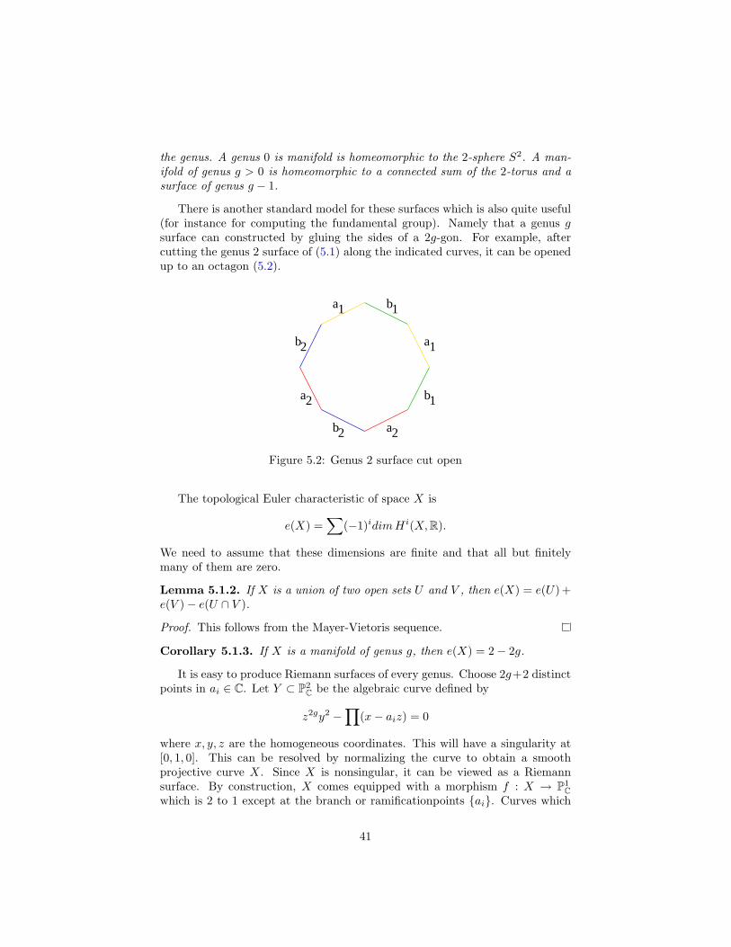
There is another standard model for these surfaces which is also quite useful(for instance for computing the fundamental group). Namely that a genus gsurface can constructed by gluing the sides of a 2g-gon. For example, aftercutting the genus 2 surface of (5.1) along the indicated curves, it can be openedup to an octagon (5.2).
a1 b1
a1
b1
b2
b2
a2
a2
Figure 5.2: Genus 2 surface cut open
The topological Euler characteristic of space X is
e(X) =∑
(−1)idim Hi(X, R).
We need to assume that these dimensions are finite and that all but finitelymany of them are zero.
Lemma 5.1.2. If X is a union of two open sets U and V , then e(X) = e(U)+e(V )− e(U ∩ V ).
Proof. This follows from the Mayer-Vietoris sequence.
Corollary 5.1.3. If X is a manifold of genus g, then e(X) = 2− 2g.
It is easy to produce Riemann surfaces of every genus. Choose 2g+2 distinctpoints in ai ∈ C. Let Y ⊂ P2
C be the algebraic curve defined by
z2gy2 −∏
(x− aiz) = 0
where x, y, z are the homogeneous coordinates. This will have a singularity at[0, 1, 0]. This can be resolved by normalizing the curve to obtain a smoothprojective curve X. Since X is nonsingular, it can be viewed as a Riemannsurface. By construction, X comes equipped with a morphism f : X → P1
Cwhich is 2 to 1 except at the branch or ramificationpoints ai. Curves which
41

can realized as two sheeted ramified coverings or P1C are rather special, and are
called hyperelliptic. In the exercises, it will be shown that the genus of X is g.Actually, we’re abusing the standard terminology, where the term hyperellipticis reserved for g > 1.
Consider the pairing
α ∧ β 7→∫
α ∧ β
on H1(X, C). This is skew symmetric and nondegnerate by Poincare duality(7.2.2). In this case, one can visualize this in terms of intersection numbers ofappropriately chosen curves on X. For example, after orientating the curvesa1, a2, b1, b2 in figure (5.1) properly, we get the intersection matrix:
0 0 1 00 0 0 1−1 0 0 00 −1 0 0
Exercise 5.1.4.
1. Let S be the toplogical space associated to a finite simplicial complex (jumpahead to the chapter 6 for the definition if necessary). Prove that e(S) isthe alternating sum of the number of simplices.
2. Check that the genus of the hyperelliptic curve constructed above is g bytriangulating in such way that the ai are included in the set of vertices.
5.2 Examples
Many examples of compact Riemann surfaces can be constructed explicitly non-singular smooth projective curves. We have already done this for hyperellipticcurves.
Example 5.2.1. Let f(x, y, z) be a homogeneous polynomial of degree d. Sup-pose that the partials of f have no common zeros in C3 except (0, 0, 0). Thenthe V (f) = f(x, y, z) = 0 in P2 is smooth. We will see later that the genus is(d− 1)(d− 2)/2. In particular, not every genus occurs.
Example 5.2.2. Suppose f(x, y, z) is only irreducible, then V (f) may have sin-gularities. After resolving singularities, e. g. by normalizing, we get a Riemmansurface. By a generic projection argument one see that every smooth algebraiccurve arises this way.
Example 5.2.3. Let f(x, y) be a polynomial, nonconstant in both x andy, suchthat the partials of f have no common zeros in C2. Projection onto the firstfactor V (f) → C exhibits it as a branched cover. This can be completed to anonsingular branched cover of P1. The genus can be calculated by the Riemann-Hurwitz formula.
42
From a different point of view, we can construct many examples as quotientsof C or the upper half plane. In fact, the uniformization theorem tells us thatall examples other than P1 arise this way.
Example 5.2.4. Let L ⊂ C be a lattice, i. e. an abelian subgroup generatedby two R-linearly independent numbers. The quotient E = C/L can be madeinto a Riemann surface (exercise 1.2.11) called an elliptic curve. Since thistopologically a torus, the genus is 1.
This is not an ellipse at all of course. It gets its name because of its relationto elliptic integrals and function. An elliptic function is a meromorphic functionon C which is periodic with respect to the lattice L. A basic example is theWeierstrass ℘-function
℘(z) =1z2
+∑
λ∈L, λ6=0
(1
(z − λ)2− 1
λ2
)This induces a map on the quotient E → P1 which is two sheeted and branchedat 4 points. One of the branch points will include ∞. We can construct a“hyperelliptic” curve E′ → P1 with the same branch points. It can be checkedthat E ∼= E′, hence E is algebraic.
The group PSL2(R) = SL2(R)/±I acts on H = z | im(z) > 0 by frac-tional linear transformations:
z 7→ az + b
cz + d
The action of subgroup Γ ⊂ PSL2(R) on H is properly discontinuous if everypoint has a neighbourhood D such that gD ∩ D 6= ∅ for all but finitely manyg ∈ Γ; it is free and properly discontinuous if g = I is the only such g.
Example 5.2.5. If Γ acts freely and properly discontinuously on H, the quotientX = H/Γ becomes a Riemann surface. If π : H → X denotes the projection,define the structure sheaf f ∈ OX(U) if and only if f π ∈ OH(π−1U).
When H/Γ is compact, the quotient has genus g > 1. The quickest wayto see this is by applying the Gauss-Bonnet theorem to the hyperbolic metric.The fundamental domain for this action will be the interior of a geodesic 2g-gon.The above construction can be extended to only properly discontinous actions.This is useful since many of the most interesting examples (e.g. SL2(Z)) dohave fixed points.
5.3 The ∂-Poincare lemma
Let U ⊂ C be an open set. Let x and y be real coordinates on C, and z = x+iy.Given a complex C∞ function f : U → C, let
∂f
∂z=
12(∂f
∂x− i
∂f
∂y)
43
∂f
∂z=
12(∂f
∂x+ i
∂f
∂y).
With this notation, the Cauchy-Riemann equation is simply ∂f∂z = 0.
In order to make it easier to globalize these operators to Riemann surfaces,we reinterpret these in terms of differential forms. In this chapter, C∞(U) andEn(U) will denote the space of complex valued C∞ functions and n-forms. Theexterior derivative extends to a C-linear operator between these spaces. Definethe complex valued 1-forms dz = dx + idy and dz = dx− idy, and set
∂f =∂f
∂zdz
∂f =∂f
∂zdz
We extend this to 1-forms, by
∂(fdz) =∂f
∂zdz ∧ dz
∂(fdz) = 0
∂(fdz) =∂f
∂zdz ∧ dz
∂(fdz) = 0
A 1-form α is holomorphic α = fdz with f holomorphic. This is equivalentto ∂α = 0. The following identities can be easity verified:
d = ∂ + ∂ (5.1)∂2 = ∂2 = 0∂∂ + ∂∂ = 0
Theorem 5.3.1. Let D ⊂ C be an open disk. Given f ∈ C∞(D), there existsg ∈ C∞(D) such that ∂g
∂z = f .
Proof. A solution can be given explicitly as
g(ζ) =1
2πi
∫D
f(z)z − ζ
dz ∧ dz
See [GH, p. 5].
5.4 ∂-cohomology
Let X be a Riemann surface, i. e. a 1-dimensional complex manifold. We writeC∞
X and E iX for the sheaves of complex valued C∞ functions and i-forms. We
define a C∞-submodule E(1,0)X ⊂ E1
X (respectively E01X ⊂ E1
X), so that for any
44

coordinate neighbourhood U holomorphic cordinate z, E(1,0)X (U) = C∞(U)dz
(resp. E(0,1)X (U) = C∞(U)dz). We have a decomposition
E1X = E(1,0)
X ⊕ E(0,1)X
We set E(1,1)X = E2
X as this is locally generated by dz ∧ dz.
Lemma 5.4.1. There exists C-linear maps ∂, ∂ on the sheaves E•X which coin-cide with the previous expressions in local coordinates.
It follows that the identities (5.1) hold globally, and the kernels of ∂ areprecisely the sheaves of holomorphic functions and forms respectively.
Lemma 5.4.2. The sequences of sheaves
0→ OX → C∞X
∂−→ E(0,1)X → 0
0→ Ω1X → E
(1,0)X
∂−→ E(1,1)X → 0
are acyclic resolutions.
Proof. Any C∞-module is soft, hence acyclic, and the exactness follows fromtheorem5.3.1.
Corollary 5.4.3.
H1(X,OX) =E(0,1)(X)∂C∞(X)
H1(X, Ω1X) =
E(1,1)(X)
∂E(1,0)X (X)
andHi(X,OX) = Hi(X, Ω1
X) = 0
if i > 1.
Next, we want a holomorphic analogue of the de Rham complex.
Proposition 5.4.4. There is an exact sequence of sheaves
0→ CX → OXd−→ Ω1
X → 0
Proof. The only nontrivial part of the assertion is that OX → Ω1X → 0 is exact.
We can check this by replacing X by a disk D. A holomorphic 1-form on Dis automatically closed, therefore exact by the usual Poincare lemma. If df isholomorphic then ∂f = 0, so f is holomorphic.
Corollary 5.4.5. There is a long exact sequence
0→ H0(X, C)→ H0(X,OX)→ H0(X, Ω1X)→ . . .
45
Holomorphic 1-forms are closed, and
H0(X, Ω1X)→ H1(X, C)
is the map which sends a holomorphic form to its class in de Rham cohomology.
Lemma 5.4.6. When X is compact and connected, this map is an injection.
Proof. It is equivalent to proving that
H0(X, C)→ H0(X,OX)
is surjective i.e. that global holomorphic functions are constant. Let f be aholomorphic function on X. f must attain a maximum at some point, sayx ∈ X. Choose a coordinate disk D ⊂ X centered at x. The we can applythe maximum modulus principle to conclude that f is constant on D. Sincef − f(x) has a nonisolated 0, it follows by complex analysis that f is globallyconstant.
In section 8.1 we will show that the dimension of H0(X, Ω1X) is exactly the
genus. For now, we prove a weak form of this statement.
Lemma 5.4.7. If X is compact and connected then dim H0(X, Ω1X) ≤ g, where
g is the genus.
Proof. As we have seen, we can view H10 = H0(X, Ω1X) as a subpsace of
H1(X, C). Given two holomorphic 1-forms α, β, α ∧ β = 0. This implies thatH10 is an isotropic subpsace under the skew symmetric Poincare duality pairing.So dim H10 ≤ 1
2dim H1(X, C) by linear algebra.
In the case of the hyperelliptic curve constructed in section 5.1, one cancheck the opposite inequallity by hand. The expressions xidx/y with 0 ≤ i < ggive g linearly elements of H0(X Ω1
X) (see exercises).One additional property whose proof will postponed to section 5.4.3 is that
the mapH1(X, C)→ H1(X,OX)
is surjective, or equivalently that H1(X, Ω1X) injects into H2(X, C). It follows
from this that dim H1(X,OX) = g. The fact that H0(X, ΩX) ∼= H1(X,OX) isusually deduced from the Serre duality theorem.
Exercise 5.4.8.
1. The differentials xidx/y on the hyperelliptic curve are certainly holomor-phic on X−Σ where Σ = f−1ai∪∞. Check that they holomorphicallyextend to Σ.
46
5.5 Projective embeddings
Fix a compact Riemann surface X. We want to assume a couple of things thatstated above but not yet proven, namely that dim H0(X, Ω1
X) and dim H1(X,OX)both coincide with the genus of X. We introduce some standard shorthand:hi = dim Hi, and ωX = Ω1
X .A divisor D on X is a finite integer linear combination
∑nipi where pi ∈ X.
One says that D is effective if all the coefficients are nonnegative. The degreedeg D =
∑ni. For every meromphic function defined in a neighbourhood of
p ∈ X, let ordp(f) be the order of vanishing (or minus the order of the pole) off at p. If D is a divisor define ordp(D) to be the coefficient of p in D (or 0 if pis absent). Define the sheaf OX(D) by
OX(D)(U) = f : U → C ∪ ∞ | ordp(f) + ordp(D) ≥ 0, ∀p ∈ U
Lemma 5.5.1. This is a line bundle.
Proof. Let U be a coordinate neighbourhood , and let D =∑
nipi + D′ wherepi ∈ U and D′ is sum of points not in U . hen we can find functions fi vanishingat each point pi ∈ U to order 1 and nowhere else. It is can be checked that
OX(D)(U) = OX(U)1
fn11 fn2
2 . . .,
which is free of rank one.
Divisors form an abelian group Div(X) in the obvious way.
Lemma 5.5.2. OX(D + D′) ∼= OX(D)⊗OX(D′).
In later terminology, this says that D 7→ OX(D) is a homomorphism fromDiv(X) → Pic(X). If D is effective O(−D) is a sheaf of ideals. In particular,OX(−p) is exactly the maximal ideal sheaf at p. We have an exact sequence
0→ OX(−p)→ OX → Cp → 0 (5.2)
where
Cp(U) =
C if p ∈ U0 otherwise
Tensoring (5.2) by OX(D) and observing that Cp⊗L ∼= Cp for any line bundle,yields
0→ OX(D − p)→ OX(D)→ Cp → 0 (5.3)
In the same way, we get a sequence
0→ ωX(D − p)→ ωX(D)→ Cp → 0 (5.4)
where ωX(D) = ωX ⊗OX(D).
Lemma 5.5.3. For all D, Hi(X,OX(D)) and Hi(X, ωX(D)) are finite dimen-sional and 0 if i > 1.
47
The statement is actually redundant, but we haven’t proved that it is.
Proof. Observe that Cp has no higher cohomology since it is flabby. (5.3) yields
0→ H0(OX(D−p))→ H0(OX(D))→ C→ H1(OX(D−p))→ H1(OX(D))→ 0
and isomorphisms
Hi(OX(D − p)) ∼= Hi(OX(D)) i > 0
By adding or subtracting points, we can reduce this to the case of OX(D) = OX .The argument for ωX(D) is the same.
The residue of a meromorphic 1-form α at p is
resp(α) =1
2πi
∫C
α
where C is any loop “going once counterclockwise” around p and containing nosingularities other than p. Alternatively, if α = f(z)dz locally for some localcoordinate z at p, resp(α) is the coefficient of 1
z in the Laurant expansion off(z).
Lemma 5.5.4 (Residue Theorem). If α is a meromorphic 1-form, it hasfinitely many singularities, and the sum of the residues is 0.
Proof. The singularities are isolated hence they form a finite set p1, . . . pn.For each i, choose an open disk Di containing pi and no other singularity. Thenby Stokes’ theorem ∑
respiα =
12πi
∫X−∪Di
dα = 0.
Theorem 5.5.5. Suppose that D is a nonzero effective divisor then
(A) H1(ωX(D)) = 0.
(B) h0(ωX(D)) = deg D + g − 1.
(A) is due to Serre. It is a special case of the Kodaira vanishing theorem.(B) is a weak form of the Riemann-Roch theorem.
Proof. (A) will be proved by induction on the degree of D. Suppose D = p.Then H0(ωX(p)) consists of the space of meromorphic 1-forms α with at worsta simple pole at p and no other singularities. The residue theorem that suchan α must be holomorphic. By the long exact sequence of cohomology groupsassociated to (5.4), we have
0→ C → H1(ωX)→ H1(ωX(p))→ 0
48

Since the space in the middle is one dimensional, this proves (A) in this case.In general, the inductive step follows from a similar application of (5.4).
(B) will again be proved by induction. As already noted when D = p,h0(ωX(D)) = h0(ωX) = g. In general, (5.4) and (A) shows
h0(ωX(D)) = 1 + h0(ωX(D − p)) = deg D + g − 1
by induction.
Corollary 5.5.6. There exists a divisor (called a canonical divisor) such thatωX∼= OX(K)
Proof. Choose D so that H0(ωX(D)) possesses a nonzero section α. Locallyα = fdz, and we define ordp(α) = ordp(f) (this is independent of the coordinatez). Then
K = (α)−D =∑
ordp(α)p−D
satisfies the required properties.
Although, we won’t prove that here, the degree of K is known.
Proposition 5.5.7. deg K = 2g − 2
We say that a line bundle L on X is globally generated if for any pointx ∈ X, there exists a section f ∈ H0(X, L) such that f(x) 6= 0. Suppose thatthis is the case, Choose a basis f0, . . . fN for H0(X, L). If fix an isomorphismτ : L|U ∼= OU , τ(fi) are holomorphic functions on U . Thus we get a holomorphicmap U → CN+1 given by x 7→ (τ(fi(x))). By our assumption, the image liesin the complement of 0, and thus descends to a map to projective space. Theimage is independent of τ , hence we get a well defined holomorphic map
φL : X → PN
This map has the property that φ∗LOPN (1) = L. L is called very ample if φL isan embedding.
Proposition 5.5.8. A sufficient condition for L to be globally generated is thatH1(X, L(−p)) = 0 for all p ∈ X A sufficient condition for L to be very ampleis that H1(X, L(−p− q)) = 0 for all p, q ∈ X
Corollary 5.5.9. ωX(D) is very ample if D is nonzero effective with degD > 2.In particular, any Riemann surface can be embedded into a projective space.
5.6 Automorphic forms
Let Γ ⊂ SL2(R) be a subgroup and k a positive integer, an automorphic formof weight 2k is a holomorphic function f : H → C on the upper half planesatisfying
f(z) = (cz + d)−2kf(az + b
cz + d)
49
for each (a bc d
)∈ Γ
Choose a weight 2k automorphic form f . Then f(z)(dz)⊗k is invariant underthe group precisely when f is automorphic of weight 2k. Since −I acts triviallyon H, the action of SL2(R) factors through PSL2(R) = SL2(R)/±I. Let ussuppose that the group Γ/±I/ acts freely, then the quotient X = H/Γ is aRiemann surface, and an automorphic form of weight 2k descends to a sectionof the sheaf ω⊗k
X . We can apply the previous to the calculate the dimensions ofthese spaces.
Proposition 5.6.1. Suppose that Γ/±I acts freely on H and that the quo-tient X = H/Γ is compact of genus g. Then the dimension of the space ofautomorphic functions of weight 2k is
g if k = 1(g − 1)(2k − 1) if k > 1
Proof. When k = 1, this is clear. When k > 1, we have
h0(ω⊗k) = h0(ω((k − 1)K)) = (k − 1)(deg K) + g − 1 = (2k − 1)(g − 1)
Our discussion so far is inadequate since it doesn’t deal with examples suchas the modular group SL2(Z). This is a particularly interesting example, sincetwo elliptic curves C/Z + Zτ and C/Z + Zτ ′, with τ, τ ′ ∈ H, are isomorphic ifand only if τ and τ ′ lie in the same orbit of SL2(Z). The quotient H/SL2(Z) isnoncompact, in fact it is can be identified with C via the j-function [S4, p. 89].The natural compactification P1 can be constructed as a quotient as follows.H has compactification by the circle R ∪ ∞ (this is easier to visualize if weswitch to the unit disk model D ∼= H), however we add only rational pointsH∗ = D∪Q∪∞ called cusps. Then SL2(Z) acts on this, and the cusps forma unique orbit corresponding the point at infinity in P1.
We can apply the same technique to any finite index subgroup of the modulargroup.
Theorem 5.6.2. Given a finite index subgroup Γ ⊂ SL2(Z), H∗/Γ can bemade into a compact Riemann surface such that H∗/Γ → H∗/SL2(Z) ∼= P1 isholomorphic.
For example, the nth principle congruence subgroup
Γ(n) =(
a bc d
)∈ SL2(Z) | a− 1 ≡ d− 1 ≡ b ≡ c ≡ 0 mod n
Γ(2)/±I acts freely on H, and the quotient is isomorphic to P1 − 0, 1,∞.In the unit disk we can choose a fundamental domain for Γ(2) as depicted infigure 5.3. The three cusps in the domain correspond to the points 0, 1,∞. Apretty consequence of this is Picard’s little theorem:
50
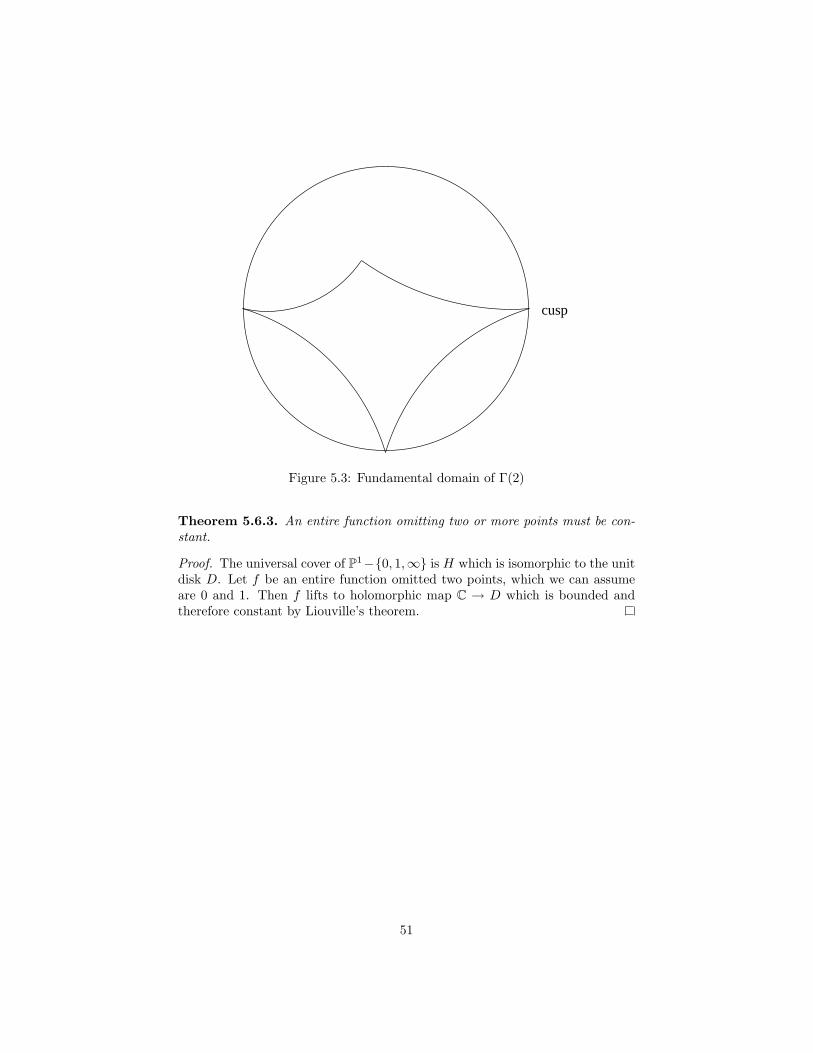
cusp
Figure 5.3: Fundamental domain of Γ(2)
Theorem 5.6.3. An entire function omitting two or more points must be con-stant.
Proof. The universal cover of P1−0, 1,∞ is H which is isomorphic to the unitdisk D. Let f be an entire function omitted two points, which we can assumeare 0 and 1. Then f lifts to holomorphic map C → D which is bounded andtherefore constant by Liouville’s theorem.
51
Chapter 6
Simplicial Methods
In this chapter, we will develop some tools for actually computing cohomologygroups in practice. All of these are based on simplicial methods.
6.1 Simplicial and Singular Cohomology
A systematic development of the ideas in this section can be found in [Sp].The standard n-simplex is
∆n = (t1, . . . tn+1) ∈ Rn+1 |∑
ti = 1, ti ≥ 0
The ith face ∆ni is the intersection of ∆n with the hyperplane ti = 0 (see
(6.1). Each face is homeomorphic an n − 1 simplex by an explicit affine mapδi : ∆n−1 → ∆n
i . More generally, we refer to the intersection of ∆ with thelinear space xi1 = . . . xik
= 0 as a face.
Some fairly complicated topological spaces, called polyhedra or triangulablespaces, can be built up by gluing simplices. It is known, although by no meansobvious, that manifolds and algebraic varieties (with classical topology) canbe triangulated. The combinatorics of the gluing is governed by a simplicialcomplex. This consists of a set V of vertices, and collection of finite nonemptysubsets Σ of V containing all the singletons and closed under taking nonemptysubsets. We can construct a space |(V,Σ)| out of this roughly as follows. Toeach maximal element S ∈ Σ, choose an n-simplex ∆(S), where n + 1 is thecardinality of S. Glue ∆(S) to ∆(S′) along the face labeled by S ∩S′ wheneverthis is nonempty. (When V is infinite, this gluing process requires some care,see [Sp, chap. 3].)
Let K = (V,Σ) be a simplical complex, and assume that V is linearly or-dered. We will refer to element of Σ as a n-simplex if it has cardinality n + 1.We define an n-cochain on a simplicial complex with values in an abelian groupA to be function which assigns an element of A to every n-simplex. One can
52

∆
∆3
3
3
Figure 6.1: 3 simplex
think of a n-cochain some sort of combinatorial analogue of an integral of n-form. As in integration theorem one needs to worry about orientations, and thisis where the ordering comes in. An alternative, which is probably more stan-dard, is to use oriented simplices; the complexes one gets this way are bigger,but the resulting cohomology theory is the same. Given an n-cochain F , wedefine a (n + 1)-cochain ∂(F ). called the coboundary or differential of F . Inanalogy with Stokes’ theorem which allows one to calculate the integral of dαas in integral along the boundary, we define
∂(F )(v0, . . . vn) =∑
(−1)iF (v0, . . . vi . . . vn),
whenever v0 < v1 . . . < vn. (The notation x means omit x.) Let Cn(K, A)denote the set of n-cochains. This is clearly an abelian group (in fact an A-module if A is ring). We extend ∂ : Cn(K, A)→ Cn+1(K, A) by linearity. Thekey relation is
Lemma 6.1.1. ∂2 = 0.
Proof. Let∂i(F )(v0, . . . vn) = F (v0, . . . vi . . . vn)
so that ∂ =∑
(−1)i∂i. The lemma follows for the easily verified identity ∂j∂i =∂i∂j−1 for i < j.
Thus we have a complex. The simplicial cohomology of K is defined by
Hi(K, A) = Hi(C•(K, A)).
Note that when V is finite, these groups are automatically finitely generatedand computable. However, triangulations of interesting spaces tend to be quitecomplicated, so this not a particularly practical method.
53
When A is replaced by a commutative ring R. There is a product on co-homology analogous to the product in De Rham induced by wedging forms.Given two cochains α ∈ Cn(K, R), β ∈ Cm(K, R), their cup product α ∪ β ∈Cn+m(K, R) is given by
α ∪ β(v0, . . . vn+m) = α(v0, . . . vn)β(vn, . . . vn+m) (6.1)
where v0 < v1 < . . .. Then:
Lemma 6.1.2. ∂(α ∪ β) = ∂(α) ∪ β + (−1)nα ∪ ∂(β)
Corollary 6.1.3. ∪ induces an operation on cohomology that makes H∗(K, R)into a graded ring.
Singular cohomology was introduced partly in order to give conceptual proofof the fact that Hi(K, A) depends only on |K|, i.e. that simplicial cohomologyis independant of the triangulation. It has the advantage, for us, that therelation with sheaf cohomology is easier to establish. A singular n-simplex on atopological space X is simply a continuous map from f : ∆n → X. When X isa manifold, we can require the maps to be C∞. We define a singular n-cochainon a X be a map which assigns an element of A to any n-simplex on X. LetSn(X, A) (Sn
∞(X, A)) denote the group of (C∞) n-cochains with values in A.When F is an n-cochain, its coboundary is the (n + 1)-cochain
∂(F )(f) =∑
(−1)iF (f δi).
The following has more or less the same proof as lemma 6.1.1.
Lemma 6.1.4. ∂2 = 0.
Thus we have a complex. The singular cohomolgy groups of X are
Hising(X, A) = Hi(S∗(X, A)).
A basic property of this cohomology theory is its homotopy invariance. We statethis in the form that we will need. A subspace Y ⊂ X is called a deformationretraction, if there exists a a continuous map F : [0, 1] × X → X such thatF (0, x) = x, F (1, X) = Y and F (1, y) = y for y ∈ Y . If Y is a point then X iscalled contractible.
Proposition 6.1.5. If Y ⊂ X is a deformation retraction, then
Hising(X, A)→ Hi
sing(Y,A)
is an isomorphism for any A.
In particular, the higher cohomology vanishes on a contractible space. Thisis an analogue of Poincare’s lemma. Call space locally contractible if everypoint has a contractible neighbourhood . Manifolds and varieties with classicaltopology are examples of such spaces.
54

Theorem 6.1.6. If X is paracompact Hausdorff space (e. g. a metric space)which is locally contractible, then Hi(X, AX) ∼= Hi
sing(X, A) for any abeliangroup A.
A complete proof can be found in [Sp, chap. 6] (note that Spanier uses Cechapproach discussed in the next chapter). In the case of manifolds, a proof whichis more natural from our point of view can be found in [Wa]. The key step isto consider the sheaves Sn associated to the presheaves U 7→ Sn(U,A). Thesesheaves are soft since they are modules over the sheaf of real valued continuousfunctions. The local contractability guarantees that
0→ AX → S0 → S1 → . . .
is a fine resolution. Thus one gets
Hi(X, AX) ∼= Hi(S∗(X))
It remains to check that the natural map
S∗(X, A)→ S∗(X)
induces an isomorphism on cohomology. We the reader refer to [Wa, pp 196-197]for this.
As a corollary, we obtain the form of De Rham’s theorem that most peoplethink of.
Corollary 6.1.7 (De Rham’s theorem, version 2). If X is a manifold,
HidR(X, R) ∼= Hi
sing(X, R)
The theorem holds with C∞ cochains. The map in the corollary can bedefined directly on the level of complexes by
α 7→ (f 7→∫
∆
f∗α)
Singular cohomology carries a cup product given by formula (6.1). A strongerform of De Rham’s theorem shows that the above map is a ring isomorphism[Wa]. Fundamental classes of oriented submanifolds can be constructed inH∗(X, Z). This explains why the the intersection numbers Y · Z were integersin proposition 4.4.2.
Exercise 6.1.8.
1. Calculate the simplicial cohomology with Z coefficients for the “tetrahe-dron” which is the powerset of V = 1, 2, 3, 4 with ∅ and V removed.
2. Let Sn be the n-sphere realized as the unit sphere in Rn+1. Let U0 =Sn − (0, . . . 0, 1) and U1 = Sn − (0, . . . 0,−1). Prove that Ui arecontractible, and that U0 ∩U1 deformation retracts on to the “equatorial”(n− 1)-sphere.
55
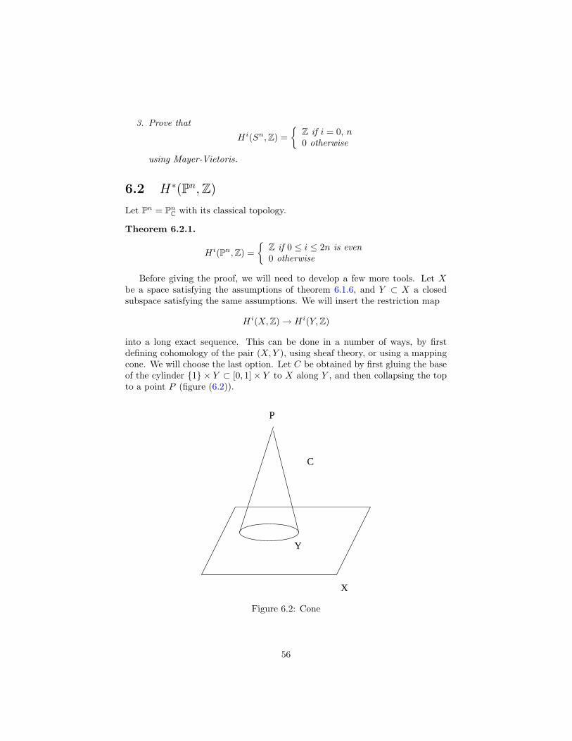
3. Prove that
Hi(Sn, Z) =
Z if i = 0, n0 otherwise
using Mayer-Vietoris.
6.2 H∗(Pn, Z)
Let Pn = PnC with its classical topology.
Theorem 6.2.1.
Hi(Pn, Z) =
Z if 0 ≤ i ≤ 2n is even0 otherwise
Before giving the proof, we will need to develop a few more tools. Let Xbe a space satisfying the assumptions of theorem 6.1.6, and Y ⊂ X a closedsubspace satisfying the same assumptions. We will insert the restriction map
Hi(X, Z)→ Hi(Y, Z)
into a long exact sequence. This can be done in a number of ways, by firstdefining cohomology of the pair (X, Y ), using sheaf theory, or using a mappingcone. We will choose the last option. Let C be obtained by first gluing the baseof the cylinder 1 × Y ⊂ [0, 1]× Y to X along Y , and then collapsing the topto a point P (figure (6.2)).
X
Y
C
P
Figure 6.2: Cone
56

Let U1 = C−P , and U2 ⊂ C the open cone [0, 1)×Y/0×Y (the notationA/B means collapse B to a point). On sees that U1 deformation retracts to X,U2 is contractible, and U1 ∩ U2 deformation retracts to Y . The Mayer-Vietorissequence, together with these facts, yields a long exact sequence
. . .Hi(C, Z)→ Hi(X, Z)→ Hi(Y, Z)→ Hi+1(C, Z) . . .
when i > 0. The make this really useful, note that the map C → C/U2 whichcollapses the closed cone to a point is a homotopy equivalence. Therefore itinduces an isomorphism on cohomology. Since we can identify C/U2 with X/Y ,we obtain a sequence
. . .Hi(X/Y, Z)→ Hi(X, Z)→ Hi(Y, Z)→ . . . (6.2)
We apply this when X = Pn and Y = Pn−1 embedded as a hyperplane. Thecomplement X − Y = Cn. Collapsing Y to a point amounts to adding a pointat infinity to Cn, thus X/Y = S2n. Since projective spaces are connected
H0(Pn, Z) ∼= H0(Pn−1, Z) ∼= Z.
For i > 0, (6.2) and the previous exercise yields isomorphisms
Hi(Pn, Z) ∼= Hi(Pn−1, Z), when i < 2n (6.3)
H2n(Pn, Z) ∼= Z
The theorem follows by induction.
Exercise 6.2.2.
1. Let L ⊂ Pn be a linear subspace of codimension i. Prove that its funda-mental class [L] generated H2i(Pn, Z).
2. Let X ⊂ Pn be a smooth projective variety. Then [X] = d[L] for some d,where L is a linear subspace of the same dimension. d is called the degreeof X. Bertini’s theorem, which you can assume, implies that there exists alinear space L′ of complementary dimension transverse to X. Check thatX · L′ = #(X ∩ L′) = d.
6.3 Cech cohomology
We return to sheaf theory proper. We will introduce the Cech approach to co-homology which has the advantage of being quite explicit and computable (andthe disadvantage of not always giving the “right” answer). Roughly speaking,Cech bears the same relation to sheaf cohomology, as simplicial does to singularcohomology.
57
One starts with an open covering Ui | i ∈ I of a space X indexed by atotally ordered set I. If J ⊆ I, let UJ be the intersection of Uj with j ∈ J . LetF be a sheaf on X. The group of Cech n-cochains is
Cn = Cn(Ui,F) =∏
i0<...<in
F(Ui0...in)
The coboundary map ∂ : Cn → Cn+1is defined by
∂(f)i0...in+1 =∑
k
(−1)kfi0...ik...in+1|Ui0...in+1
where i signifies that i should be omitted. This satisfies ∂2 = 0. So we candefine the nth Cech cohomology group as
Hn(Ui,F) = Hn(C•) =ker(∂ : Cn → Cn+1)im(∂ : Cn−1 → Cn)
To get a feeling for this, let us write out the first couple of groups explicitly:
H0(Ui,F) = (fi) ∈∏F(Ui) | fi = fj on Uij
= F (X)
H1(Ui,F) =(fij) ∈
∏F(Uij) | fik = fij + fjk on Uijk
(fij | ∃(φi), fij = φi − φj(6.4)
There is a strong similarity with simplicial cohomology. This can be madeprecise by introducing a simplicial complex called the nerve of the covering. Forthe set of vertices, we take the index set I. The set of simplices is given by
Σ = i0, . . . in |Ui0,...in 6= ∅
If we assume that each Ui0,...inis connected, then we see that the Cech complex
Cn(Ui, AX) coincides with the simplicial complex of the nerve with coefficientsin A.
Even though, we are primarily interested in sheaves of abelian groups. Itwill be convenient to extend (6.4) to a sheaf arbitrary groups G.
H1(Ui,G) = (gij) ∈∏i<j
G(Uij) | gik = gijgjk on Uijk /∼
where (gij) ∼ (gij) if there exists (γi) ∈∏G(Ui) such that gij = γigijγ
−1j . Note
that this is just a set in general. The (gij) are called 1-cocycles with values inG. It will be useful to drop the requirement that i < j by setting gji = g−1
ij andgii = 1.
As an example of sheaf of nonabelian groups, take U 7→ GLn(R(U)), where(X,R) is a ringed space (i.e. space with a sheaf of commutative rings).
58
Theorem 6.3.1. Let (X,R) be a manifold or a variety over k, and Ui andopen cover of X. There is a bijection between the following sets:
1. The set of isomorphism classes of rank n vector bundles over (X,R) triv-iallizable over Ui.
2. The set of isomorphism classes of locally free R-modules M of rank n suchM |Ui
is free.
3. H1(Ui, Gln(R)).
Proof. We merely describe the correspondences.1→ 2: Take the sheaf of sections.2 → 3: Given M as above. Choose isomorphisms Fi : Rn
Ui→ M |Ui
.Setgij = Fi F−1
j . This determines a well defined element of H1.3→ 1: Define an equivalence relation ∼ on the disjoint union W =
∐Ui×kn
as follows. Given (xi, vi) ∈ Ui × kn and (xj , vj) ∈ Uj × kn, (xi, vi) ∼ (xj , vj)iff xi = xj and vi = gij(x)vj . Let V = W/ with quotient topology. Given anopen set U ′/ ∼= U ⊂ V . Define f : U → k to be regular, C∞ or holomorphic(as the case may be) if its pullback to U ′ has this property.
Implicit above, is a construction which associates to a 1-cocycle γ = (gij),the locally free sheaf
Mγ(U) = (vi) ∈∏R(U ∩ Ui)n | vi = gijvj.
Consider the case of projective space P = Pnk . Suppose x0, . . . xn are homoge-
neous coordinates. Let Ui be the complement of the hyperplane xi = 0. ThenUi is isomorphic to An
k by
[x0, . . . xn]→ (x0
xi, . . .
xi
xi. . .)
Define gij = xj/xi ∈ O(Uij)∗. This is a 1-cocycle, and Mgij∼= OP(1). Likewise
(xj/xi)d is the 1-cocyle for O(d).We get rid of the dependence on coverings by taking direct limits. If Vj is
refinement of Ui, there is a natural restriction map
Hi(Ui,F)→ Hi(Vj,F)
We defineHi(X,F) = lim
→Hi(Ui,F)
Corollary 6.3.2. There is a bijection between the following sets:
1. The set of isomorphism classes of rank n vector bundles over (X,R).
2. The set of isomorphism classes of locally free R-modules M of rank n.
3. H1(X, Gln(R)).
59
A line bundle is a rank one vector bundle. We won’t distinguish betweenlines bundles and rank one locally free sheaves. The set of isomorphism classesof line bundles carries the stucture of a group namely H1(X,R∗). This groupis called the Picard group, and is denoted by Pic(X).
Exercise 6.3.3.
1. Check the description of OP(1) given above.
2. Show that multiplication in Pic(X) can be interpreted as tensor productof line bundles.
6.4 Cech versus sheaf cohomology
Definition 6.4.1. An open covering Ui is called a Leray covering for a sheafF if Hn(UJ ,F) = 0 for all nonempty finite sets J and n > 0.
Lemma 6.4.2. Suppose that H1(UJ , A) = 0 for all nonempty finite sets J .Then given an exact sequence
0→ A→ B → C → 0
of sheaves, there is a long exact sequence:
0→ H0(Ui, A)→ H0(Ui, B)→ H0(Ui, C)→ H1(Ui, A) . . .
Proof. The hypothesis guarantees that there is a short exact sequence of com-plexes:
0→ C•(Ui, A)→ C•(Ui, B)→ C•(Ui, C)→ 0.
The long exact now follows from a standard result in homological algebra...
Lemma 6.4.3. Suppose that F is flabby, then Hn(F) = 0 for all n > 0.
Theorem 6.4.4. If Ui is a Leray with respect to F then
Hn(Ui,F) ∼= Hn(X,F)
Proof. This is clearly true for n = 0. Next consider the case where n = 1.Lemmas 6.4.2 and 6.4.3 imply that
H1(F) = coker[Γ(X, G(F))→ Γ(X, C1(F))] = H1(X,F).
The remaining cases follow by dimension shifting, e.g.
H2(F) = H1(C1(F)) = H2(X,F)
We state few more general results.
60
Proposition 6.4.5. For any sheaf F
H1(X,F) ∼= H1(X,F)
Proof. See [G, Cor. 5.9.1]
Theorem 6.4.6. If X is a paracompact space then for any sheaf and all i,
Hi(X,F) ∼= Hi(X,F)
Proof. See [G, Cor. 5.10.1]
6.5 First Chern class
Let (X,OX) be a complex manifold or algebraic variety over C. Then we haveisomorphisms
Pic(X) ∼= H1(X,O∗X) ∼= H1(X,O∗X)The exponential sequence is
0→ ZX → OXe2πi
−→ O∗X → 1 (6.5)
Definition 6.5.1. Given a line bundle L, its first Chern class c1(L) ∈ H2(X, Z)is the image of L under the connecting map Pic(X)→ H2(X, Z)
This can be carried out for C∞ manifolds as well. Provided one interpretsOX as the sheaf of complex valued C∞ functions, and Pic(X) as group of C∞
complex line bundles. In this case, c1 is an isomorphism. It is clear that theconstruction is functorial:
Lemma 6.5.2. If f : X → Y is C∞ map between manifolds, c1(f∗L) =f∗c1(L).
We want to calculate this explicitly for P = P1C. We can use the standard
covering Ui = xi 6= 0. We identify U1 with C with the coordinate z =x0/x1. The 1-cocycle (section 6.3) of O(1) is g01 = z−1. The logarithmicderivative dlog g01 = −dz/z is 1-cocycle with values in E1. Since this sheaf issoft, this cocycle is coboundary, i.e. there exists forms αi ∈ E1(Ui) such that−dz/z = α1 − α0 on the intersection. There dαi patch to yield a global 2-formβ ∈ E2(P). β/2πi gives an explicit representative of the image of C1(O(1)) inH2(X, C). We have an isomorphism of this space with C given by integration. Inorder to evaluate the integral
∫P β/2πi, divide the sphere into two hemispheres
H0 = |z| ≤ 1 and H1 = ‖z| ≥ 1. Let C be the curve |z| = 1 with positiveorientation. Note the boundary of H1 is −C. Then with the help of Stokes’theorem, we get
12πi
∫Pβ =
12πi
(∫
H0
dα0 +∫
H1
dα1)
=1
2πi(∫
C
α0 −∫
C
α1)
=1
2πi
∫C
dz
z= 1
61
Thus c1(O(1)) is the fundamental class of H2(P1, Z). By the same kind ofargument, we obtain:
Lemma 6.5.3. If D is a divisor on a compact Riemann surface X, c1(O(D)) =deg(D)[X]
Since c1 is compatible with restriction, (6.3) implies that the same holds forPn:
Lemma 6.5.4. c1(OPn(1)) = [H] where H ⊂ Pn is a hyperplane.
62
Chapter 7
The Hodge theorem
Thus far, our approach has been pretty much algebraic or topological. Weare going to need a basic analytic result, namely the Hodge theorem whichsays that every de Rham cohomology class has a unique “smallest” element.Standard acccounts of basic Hodge theory can be found in the books of Griffiths-Harris [GH], Warner [Wa] and Wells [W]. However, we will depart slightlyfrom these treatments by outling the heat equation method of Milgram andRosenbloom [MR]. This is an elegant and comparatively elementary approachto the Hodge theorem. As a warm up, we will do a combinatorial version whichrequires nothing more than linear algebra.
7.1 Hodge theory on a simplicial complex
In order to motivate the general Hodge theorem, we work this out for a finitesimplicial complex. This will require nothing beyond linear algebra
Let K = (V,Σ) be a finite simplicial complex. Choose inner products on thespaces of cochains C∗(K, R). For each simplex S, let
δS(S′) =
1 if S = S′
0 otherwise
These form a basis. A particularly natural choice of inner product is determinedby making this basis orthonormal. Let ∂∗ : Ci(K, R) → Ci−1(K, R) be theadjoint to ∂, and let ∆ = ∂∂∗ + ∂∗∂. ∆ is the discrete Laplacian.
Lemma 7.1.1. Let α be a cochain. The following are equivalent:
1. α ∈ (im∂)⊥ ∩ ker∂.
2. ∂α = ∂∗α = 0.
3. ∆α = 0.
The cochains satisfying the above conditions are called harmonic.
63
Lemma 7.1.2. Every simplical cohomology class has a unique harmonic repre-sentative. These are precise the elements of smallest norm.
Proof. One sees that the obvious map
(im∂)⊥ ∩ ker∂ → Hn(K, R)
is an isomorphism. Given an element α in the lefthand space
||α + ∂β||2 = ||α||2 + ||∂β||2 > ||α||2
unless ∂β = 0.
Exercise 7.1.3.
1. Prove lemma 7.1.1.
2. Prove that ∆ is a positive semidefinite symmetric operator.
3. Use this to prove that limit of the “heat kernel”
H = limt→∞
e−t∆
is the orthogonal projection to the space of harmonic cochains.
7.2 Harmonic forms
Let X be an n dimensional compact oriented manifold. We want to provean analogue of lemma 7.1.2 for de Rham cohomology. In order to formulatethis, we need inner products. A Riemannian metric (, ), i.e. a family of innerproducts on the tangent spaces which vary in a C∞ fashion. The existence isstandard partition of unity argument [Wa]. A metric determines inner productson exterior powers of the cotangent bundle which will also be denoted by (, ).X possesses an differential form dvol ∈ En(X) called the volume form whichis roughly the square root of the determinant of the metric (this requires anorientation). The Hodge star operator is a C∞(X)-linear operator ∗ : Ep(X)→En−p(X), determined by
α ∧ ∗β = (α, β)dvol.
One can choose a local orthonormal basis or frame ei for E1X in a neighbourhood
of any point. Then ∗ is easy to calculate in this frame, e.g. ∗e1 ∧ . . . ek =ek+1 ∧ . . . en. From this one can check that ∗∗ = ±1. The spaces Ep(X) carryinner products:
< α, β > =∫
X
(α, β)dvol =∫
X
α ∧ ∗β
and hence norms.Then basic result of Hodge (and Weyl) is:
64
Theorem 7.2.1. Every de Rham cohomology class has a unique representativewhich minimizes norm. This is called the harmonic representative.
As an application of this theorem, we have get a new proof of a Poincareduality in strengthened form.
Corollary 7.2.2. (Poincare duality, version 2). The pairing
Hi(X, R)×Hn−i(X, R)→ R
induced by (α, β) 7→∫
α ∧ β is a perfect pairing
Proof. ∗ induces an isomorphism between the space of harmonic i-forms andn−i-forms. This proves directly that Hi(X, R) and Hn−i(X, R) are isomorphic.
Consider the map
λ : Hi(X, R)→ Hn−i(X, R)∗
given by λ(α) = β 7→∫
α ∧ β. We need to prove that λ is an isomorphism.Since these spaces have same dimension, it is enough to prove that ker(λ) = 0.But this clear since λ(α)(∗α) 6= 0 whenver α is a nonzero harmonic form.
To understand the meaning of this condition, we can find the Euler-Lagrangeequation. Let α be a harmonic p-form. Then for any for any (p− 1)-form β, wewould have to have
d
dt||α + tdβ||2|t=0 = 2 < α, dβ >= 2 < d∗α, β >= 0,
which forces d∗α = 0, where d∗ is adjoint to d. A straight forward integrationby parts shows that d∗ = ± ∗ d∗. Thus harmonicity can be expressed as a pairof differential equations dα = 0 and d∗α = 0. It’s sometimes more convenient tocombine these into a single equation ∆α = 0 where ∆ = d∗d+ dd∗ is the HodgeLaplacian. The equivalence follows from the identity < ∆α, α >= ||dα||2 +||d∗α||2.
The hard work is contained in the following:
Theorem 7.2.3. There are linear operators H (harmonic projection) and G(Green’s operator) taking C∞ forms to C∞ forms, which are characterized bythe following properties
1. H(α) is harmonic,
2. G(α) is orthogonal to the space of harmonic forms,
3. α = H(α) + ∆G(α),
for any C∞ form α.
65
Let’s see how to prove the existence part of theorem 7.2.1 given this result.Any α can be written as α = β +dd∗γ +d∗dγ with β harmonic. All these termsare in fact orthogonal to each other, so
||d∗dγ||2 =< d∗dγ, α >=< dγ, dα >,
and this vanishes if α is closed. Therefore α is cohomologous to the harmonicform β. The uniqueness is straightforward: if β′ is another harmonic represen-tative, then β − β′ is both exact and harmonic. Denoting this by dγ, we thenhave ||dγ||2 =< d∗dγ, γ >= 0.
It will be useful to record part of this argument as a corollary.
Corollary 7.2.4. There is an orthogonal direct sum
E i(X) = (harmonic forms)⊕ dE i−1(X)⊕ E i+1(X)
Before doing the general case, let’s work out the easy, but instructive, ex-ample of the torus X = Rn/Zn, with the Euclidean metric. A differential formα can be expanded in a Fourier series
α =∑
λ∈Zn
∑i1<...<ip
aλ,i1...ipe2πiλ·xdxi1 ∧ . . . ∧ dxip (7.1)
By direct calculation, one finds the Laplacian
∆ = −∑ ∂2
∂x2i
,
the harmonic projection
H(α) =∑
a0,i1...ipdxi1 ∧ . . . ∧ dxip
and Green’s operator
G(α) =∑
λ∈Zn−0
∑ aλ,i1...ip
4π2|λ|2e2πiλ·xdxi1 ∧ . . . ∧ dxip .
Since the image of H are forms with constant coefficients, this proves propos-tion 4.5.1.
7.3 Heat Equation
We will sketch an approach to 7.2.3 using the heat equation due Milgram andRosenbloom ([MR] [Ch] ). The heuristic behind it is that if α is thought of as aninitial temperature, then the temperature should approach a harmonic steadystate as the manifold cools. So our task is to solve the heat equation:
∂A(t)∂t
= −∆A(t) (7.2)
A(0) = α (7.3)
66
for all t > 0, and study the behaviour as t→∞. For simplicial complexes, thiswas the content of the previous exercise. Before describing this, we make a fewgeneral remarks. If A(t) is a C∞ solution of 7.2, upon differentiating ||A(t)||2we obtain:
2 <∂A
∂t,A >= −2 < ∆A,A >= −2(||dA||2 + ||d∗A||2) ≤ 0.
This implies that ||A||2 is nonincreasing. Therefore if A(0) = 0, it remains 0.This proves the uniqueness because the equation is linear. For existence, it isenough to prove that there exists ε independent of α, such that solutions existfor all 0 < t < ε. For if T is the supremum of the t0 for which the abovesystem has a solution for t < t0. Then T must be ∞, since otherwise pickingT − ε/2 < t0 < T and using A(t0) as the new initial condition, we see that Acan be extended to the interval t < T + ε/2.
The starting point for the proof of existence is the observation that when Xis replaced by Euclidean space and α is a compactly supported function, thenone has an explicit solution
A(t) =∫
Rn
K(x, y, t)α(y)dy
where the heat kernel
K(x, y, t) = (4πt)−n/2e−||x−y||2/4t
This can be modified to make sense for a p-form on X. When working with formson X×X, we will abuse notation a bit and write them as local expressions suchas η(x, y). Then dxη(x, y) etcetera will indicate that the operations d . . . arepreformed with y treated as a constant (or more correctly, these operations arepreformed fiberwise along the second projection). Let dist(x, y)2 be a nonneg-ative C∞ function which agrees with the square of the Riemannian distancefunction in neighbourhood of the diagonal. Let β = − 1
2dxdydist(x, y)2 and set
K(x, y, t) = (4πt)−n/2e−dist(x,y)2/4tβp
This is only an approximation to the true heat kernel on X, however one can stillget some useful information from it. For small t, it behaves like the Euclideanheat kernel, in particular in the limit it acts like a δ-function along the diagonal:
limt→0
< A(y, τ),K(x, y, t) >y= A(x, τ)
This together with the self adjointness of ∆ and integration by parts shows thatfor any p-form A on X × [0,∞)
A(x, t) = < A(x, 0),K(x, y, t) >y +∫ t
0
< K1(x, y, t), A(y, t) >y dt
−∫ t
0
< K(x, y, t), (∆y + ∂/∂t)A(y, t) >y dt
67
whereK1(x, y, t) = (∆y − ∂/∂t)K(x, y, t).
In particular, if A is a solution to equations 7.2 and 7.3, then it satisfies theintegral equation
A =< α(x),K(x, y, t) >y +∫ t
0
< K1(x, y, t), A(y, t) >y dt (7.4)
and conversely a solution to this equation satisfies the heat equation. Let Rt(A)denotes the right hand side of the above equation which we can regard as anoperator acting on forms on X× [0, t]. ||K1(x, y, t)|| is known to be bounded bya constant M independent of y and t [MR]. This implies that for t < ε = 1/M ,Rt is a contraction operator. Thus there is a fixed point, and it is C∞ becauseK is. So by the above remarks, we have a C∞ solution for all t > 0.
Since we have established existence and uniqueness of 7.2 and 7.3, the opera-tor T (α) = A(t) is well defined. One has the semigroup property Tt1+t2 = Tt1Tt2
because A(t1+t2) can be obtained by solving the heat equation with initial con-dition A(t2) and then evaluating it at t = t1. We claim, furthermore that Tt isformally selfadjoint. To see this, calculate
∂
∂t< Ttη, Tτξ >=<
∂
∂tTtη, Tτξ >=< ∆Ttη, ξ >
=< η, Tτ∆ξ >=< Ttη,∂
∂τTτξ >=
∂
∂τ< Ttη, Tτξ >
which implies that < Ttη, Tτξ > can be written as a function of t + τ , sayg(t + τ). Therefore < Ttη, ξ >= g(t) =< η, ξ >. These properties imply thatfor h ≥ 0 we have
||Tt+2hα− Ttα||2 = ||Tt+2hα||2 + ||Ttα||2 − 2 < Tt+2hα, Ttα >
= ||Tt+2hα||2 + ||Ttα||2 − 2||Tt+hα||2
= (||Tt+2hα|| − ||Ttα||)2 − 2(||Tt+hα||2 − ||Tt+2hα|| · ||Ttα||)
||Ttα||2 converges because it is nonincreasing. Therefore the above expressioncan be made arbitrarily small for large enough t. This implies that Ttα convergesin the L2 sense to an L2 form H(α). In fact, a little more work shows uniformconvergence.
We’ll outline the remaining steps. Equation 7.4 and the semigroup lawimplies the relation Tt−τα = RτTtα. In the limit as t → ∞, we get H(α) =RτH(α) which implies that Hα is C∞ and harmonic. ||Ttα−Hα|| can be shownto decay rapidly, so the integral
G(α) =∫ ∞
0
(Ttα−Hα)dt
is well defined. We’ll verify formally that this is Green’s operatorr:
∆G(α) =∫ ∞
0
∆Ttαdt = −∫ ∞
0
∂Ttα
∂tdt = α−H(α),
68
and for β harmonic
< G(α), β >=∫ ∞
0
< (Tt −H)α, β > dt =∫ ∞
0
< α, (Tt −H)β > dt = 0
as required.
Let’s return to the example of a torus X = Rn/Zn, where things can becalculated explicitly. Given α as in (7.1), the solution to the heat equation withinitial value α is given by
Ttα =∑
λ∈Zn
∑aλ,i1...ip
e(2πiλ·x−4π2|λ|2t)dxi1 ∧ . . . ∧ dxip,
and this converges to the harmonic projection
H(α) =∑
a0,i1...ipdxi1 ∧ . . . ∧ dxip
Ttα−Hα can be integrated term by term to obtain Green’s operator
G(α) =∑
λ∈Zn−0
∑ aλ,i1...ip
4π2|λ|2e2πiλ·xdxi1 ∧ . . . ∧ dxip
.
69
Chapter 8
Toward Hodge theory forComplex Manifolds
In this chapter, we take the first few steps toward Hodge theory in the complexsetting. This is really a warm up for the next chapter.
8.1 Riemann Surfaces Revisited
This section is a warm up for things to come. We also tie up a few looseends from chapter 5. Fix a compact Riemann surface X. In order to applythe techniques from the previous chapter, we need a metric which is a C∞
family of inner products. But we need to impose a compatability condition.As one learns in first course in complex analysis, conformal maps are anglepreserving, and this means that we have a well defined notion of the anglebetween two tangent vectors. Among other things, compatability will meanthat the angles determined by the metric agree with the ones above. To saythis more precisely, view X as two dimension real C∞ manifold. Choosing ananalytic local coordinate z in a neighbourhood of U , the vectors v1 = ∂/∂x andv2 = ∂/∂y give a basis (or frame) of the real tangent sheaf T R
X of X restrictedto U . The automorphism Jp : T R
X |U → T RX |U represented by(
0 1−1 0
)in the basis v1, v2 is independent of this basis, and hence globally well defined. ARiemannian metric (, ) is compatible with the complex structure, or hermitean,if the transformations Jp are orthogonal. In terms of the basis v1, v2 this forcesthe matrix of the bilinear (, ) to be a positive multiple of I by some function h.Standard partition of unity arguments show that hermitean metrics exist. Fixone. In coordinates, the metric would be represented by a tensor h(x, y)(dx ⊗dx + dy ⊗ dy). The volume form (which is globally well defined) is represented
70
by hdx ∧ dy. It follows that ∗dx = dy and ∗dy = −dx. In other words, ∗ is thetranspose of J which is independent of h. Once we have ∗, we can define all theprevious operators and talk about harmonicity. After having made such a fussabout metrics, it turns out that for our purposes one is as good as any other(for the statements though not the proofs).
Lemma 8.1.1. A 1-form is harmonic if and only if its (1, 0) and (0, 1) partsare respectively holomorphic and antiholomorphic.
Proof. A 1-form α is harmonic if and only if dα = d ∗ α = 0. Given a localcoordinate z, it can be checked that ∗dz = −idz and ∗dz = idz. Therefore the(1, 0) and (0, 1) parts of a harmonic 1-form α are closed. If α is a (1, 0)-form,then dα = ∂α. Thus α is closed if and only if it is holomorphic. Conjugationyields the analogous statement for (0, 1)-forms.
Corollary 8.1.2. dim H0(X, Ω1X) equals the genus of X.
Proof. The first Betti number dim H1(X, C) is the dimension of the spaces ofholomorphic and antiholomorphic forms, and both these spaces have the samedimension.
Lemma 8.1.3. The image of ∆ and ∂∂ on E2(X) coincide.
Proof. Computing in local coordinates yields
∂∂f = − i
2
(∂2f
∂x2+
∂2f
∂y2
)dx ∧ dy
and
d ∗ df =(
∂2f
∂x2+
∂2f
∂y2
)dx ∧ dy.
This finishes the proof because ∆ = −d ∗ d∗.
Proposition 8.1.4. The map H1(X,OX)→ H1(X, Ω1X) induced by d vanishes.
Proof. We use the use the ∂-cohomology descriptions of these spaces 5.4.3.Given α ∈ E01(X), let β = dα. We have to show that β lies in the imageof ∂. Applying theorem 7.2.3 we can write β = H(β)+∆G(β). Since β is exact,we can conclude that H(β) = 0 by corollary 7.2.4. Therefore β lies in the imageof ∂∂ = −∂∂.
Corollary 8.1.5. The map H1(X, C)→ H1(X,OX) is surjective.
8.2 Dolbeault’s theorem
We now extend the results from Riemann surfaces to higher dimensions. Givenan n dimensional complex manifold X, let OX denote the sheaf of holomorphicfunctions. We can regard X as a 2n dimensional (real) C∞ manifold as explainedin section 1.2. As with Riemann surfaces, from now on C∞ and Ek
X will denote
71
the sheaves of complex valued Ci functions and forms. We use the notationC∞
X,R and EkX,R to denote the sheaf of real valued C∞ functions and k-forms.
More formally,Ek
X(U) = C⊗R EkX,R(U).
This implies that this space has complex conjugation given by a⊗ α = a ⊗ α.Recall that Ωp
X is the sheaf of holomorphic k-forms. This is a subsheaf of EpX .
Definition 8.2.1. Let E(p,0)X (U) denote the C∞(U) submodule of Ep(U) gener-
ated by ΩpX(U). Let E(0,p)
X (U) = E(p,0)X (U), and E(p,q)
X (U) = E(p,0)X (U)∧E(0,q)
X (U).
Suppose U ⊂ Cn is an open subset. Let z1, . . . zn be the coordinates on Cn.Then E(p,q)
X (U) is a free C∞(U)-module with a basis
dzi1 ∧ . . . dzip∧ dzj1 ∧ . . . dzjq
| i1 < . . . < ip, j1 < . . . < jq
To simplify formulas, we’ll write this the above forms as dzI ∧ dzJ .All of the operations of sections 5.3 and 5.4 can be extended to the higher
dimensional case. The operators
∂ : E(p,q)X → E(p+1,q)
X
and∂ : E(p,q)
X → E(p,q+1)X
are given locally by
∂(∑I,J
fI,JdzI ∧ dzJ) =∑I,J
n∑i=1
∂fI,J
∂zidzI ∧ dzJ
∂(∑I,J
fI,JdzI ∧ dzJ) =∑I,J
n∑j=1
∂fI,J
∂zjdzI ∧ dzJ
The identities
d = ∂ + ∂ (8.1)∂2 = ∂2 = 0∂∂ + ∂∂ = 0
hold.The analogue of theorem 5.3.1 is
Theorem 8.2.2. Let D ⊂ Cn be an open polydisk (i.e. a product of disks).Given α ∈ E(p,q)(D) with ∂α = 0, there exists β ∈ C∞(D) such that α = ∂β
See [GH]. Let ΩpX be sheaf of holomorphic p-forms which are given locally
as sums of fdzI with f holomorphic. One checks immediately that this is thekernel of the ∂ operator on E(p,0)
X .
Corollary 8.2.3 (Dolbeault’s Theorem).
0→ ΩpX → E
(p,0)X
∂−→ E(p,1)X . . .
is a fine resolution.
72
8.3 Complex Tori
A complex torus is a quotient X = V/L of a finite dimensional complex vectorspace by a lattice (i.e. a discrete subgroup of maximal rank). Thus it is both acomplex manifold and a torus. Let us identify V with Cn. Let z1, . . . zn be thestandard complex coordinates on Cn, and let xi = Re(zi), yi = Im(zi).
We have already seen that harmonic forms with respect to the flat metricare the forms with constant coefficients. The space of harmonic forms can bedecomposed into (p, q) type.
H(p,q) =⊕
#I=p,#J=q
CdzI ∧ dzJ
These forms are certainly ∂-closed. Thus we get a map to ∂-cohomology.
Proposition 8.3.1. This map induces an isomorphism H(p,q) ∼= Hq(X, ΩpX).
The isomorphism V ∼= L⊗R induces a natural real structure on V . Thereforeit makes sense to speak of antilinear maps from V to C; let V ∗ denote the spaceof these.
Corollary 8.3.2. Hq(X, ΩpX) ∼= ∧qV ⊗ ∧pV ∗
It’s possible to give a fairly elementary proof of this proposition [MA]. How-ever, we will indicate the that generalizes well.
Let ∂∗ and ∂∗ denote the adjoints to ∂ and ∂ respectively (note that thisconvention is reversed in [GH]). These operators can be calculated explicitly.Let ik and ik denote contraction with the vector fields 2∂/∂zk and 2∂/∂zk.These are the adjoints to dzk∧ and dzk∧. Then
∂∗α = −∑ ∂
∂zkikα
∂∗α = −∑ ∂
∂zkikα
We can define the ∂ and ∂-Laplacians by
∆∂ = ∂∗∂ + ∂∂∗,
∆∂ = ∂∗∂ + ∂∂∗
Theorem 8.3.3. ∆ = 2∆∂ = 2∆∂ .
Proof of proposition 8.3.1. By Dolbeault’s theorem
Hq(X, ΩpX) ∼=
ker[∂ : E(p,q)(X)→ E(p, q + 1)]im[∂ : E(p,q−1)(X)→ E(p, q)]
Let α be a ∂-closed (p, q)-form. Decompose
α = β + ∆γ = β + 2∆∂γ = β + ∂γ1 + ∂∗γ2
73
with β harmonic by theorem7.2.3.
||∂∗γ2||2 =< γ2, ∂∂∗γ2 >=< γ2, ∂α >= 0.
Therefore the ∂-class of α is represented by β. The uniqueness can be provedby arguments identical to those of section 7.2. Briefly, suppose β′ is anotherharmonic form representing this class. Then β−β′ = ∂η must be orthogonal toitself.
Introduce the operators
ω =√−12
∑dzk ∧ dzk =
∑dxk ∧ dyk
Lα = ω ∧ α
and
Λ = −√−12
∑ikik
A straight forward computation yields the first order Kahler identities:
Proposition 8.3.4. If [A,B] = AB −BA then
1. [Λ, ∂] = −i∂∗
2. [Λ, ∂] = i∂∗
Proof. [GH, p. 114].
Upon substituting these into the definitions of the various laplacians someremarkable cancelations take place, and we obtain:
Proof of theorem 9.2.1. We first establish ∂∂∗ + ∂∗∂ = 0,
i(∂∂∗ + ∂∗∂) =
= ∂(Λ∂ − ∂Λ)− (Λ∂ − ∂Λ)∂
= ∂Λ∂ − ∂Λ∂ = 0
Similarly, ∂∗∂ + ∂∂∗ = 0.Next expand ∆,
∆ = (∂ + ∂)(∂∗ + ∂∗) + (∂∗ + ∂∗)(∂ + ∂)
= (∂∂∗ + ∂∗∂) + (∂∂∗ + ∂∗∂) + (∂∂∗ + ∂∗∂) + (∂∗∂ + ∂∂∗)
= ∆∂ + ∆∂
Finally, we check ∆∂ = ∆∂ ,
−i∆∂ = ∂(Λ∂ − ∂Λ) + (Λ∂ − ∂Λ)∂
= ∂Λ∂ − ∂∂Λ + Λ∂∂ − ∂Λ∂
= (∂Λ− Λ∂)∂ + ∂(∂Λ− Λ∂) = −i∆∂
74
Chapter 9
Kahler manifolds
In this chapter, we extend the results of the previous section to an importantclass of manifolds called Kahler manifolds.
9.1 Kahler metrics
Let X be a compact complex manifold with complex dimension n. Fix a her-mitean metric H, which is a choice of hermitean inner product on the complextangent spaces which vary in C∞ fashion. More precisely, H would be givenby a section of the E(1,0)
X ⊗E(0,1)X , sthat in some (any) locally coordinate system
around each point is given by
H =∑
hijdzi ⊗ dzj
with hij positive definite hermitean. By standard linear algebra, the real andimaginary parts of hij are respectively symmetric positive definite and non-degenerate skew symmetric matrices. Geometrically, the real part is just aRiemannian structure, while the (suitably normalized) imaginary part of givesa (1, 1)-form ω called the Kahler form; in local coodinates
ω =√−12
∑hijdzi ∧ dzj .
X has a canonical orientation, so the Hodge star operator associated to theRiemannian structure can be defined. ∗ will be extended to C-linear operatoron EX , and set ∗(α) = ∗α. ∗ is compatible with the natural bigrading on formsin the sense that
∗E(p,q)(X) ⊆ E(n−q,n−p)(X).
Let ∂∗ = −∗∂∗ and ∂∗ = −∗∂∗. These are adjoints of ∂ and ∂. Then we candefine the operators
∆∂ = ∂∗∂ + ∂∂∗,
75

∆∂ = ∂∗∂ + ∂∂∗
L = ω∧
Λ = − ∗ L∗
A form is called ∂-harmonic if it lies in the kernel of ∆∂ . For a general hermiteanmanifold there is no relation between harmonicity and ∂-harmonicity. However,these notions do coincide for the class the class of Kahler manifolds, which wewill define shortly.
A hermitean metric on X is called Kahler if there exist analytic coordinatesabout any point, for which the metric becomes Euclidean
hij = δij + O(z21 , z1z2 . . .)
up to second order. This implies that the Kahler form is closed: dω = 0, andin fact this is an equivalent condition [GH, p 107]. A Kahler manifold is acomplex manifold with a Kahler metric. Standard examples of compact Kahlermanifolds are:
Example 9.1.1. Riemann surfaces with any hermitean metric since dω van-ishes for trivial reasons.
Example 9.1.2. Complex tori with flat metrics.
Example 9.1.3. Pn with the Fubini-Study metric. This is the unique metricwith Kahler form which pulls back to
i
2π∂∂ log(|z0|2 + . . . |zn|2)
under the canonical map Cn+1 − 0 → Pn.
Example 9.1.4. Complex submanifolds of Kahler manifolds inherit Kahlermetrics where the Kahler class is the restriction Kahler class of the ambientmanifold. In particular, any smooth projective variety possess a (nonunique)Kahler metric.
9.2 The Hodge decomposition
Fix a Kahler manifold X. Theorem 8.3.3 generalizes:
Theorem 9.2.1. ∆ = 2∆∂ = 2∆∂ .
Proof. Since Kahler metrics are Euclidean up to second order, any identityinvolving geometrically defined first order operators on Euclidean space can beautomatically extended to Kahler manifolds. Thus proposition 8.3.4 extends.The rest of the argument is the same as in section 8.3.
This actually characterizes Kahler manifolds.
76
Corollary 9.2.2. If X is compact then Hq(X, ΩpX) is isomorphic the space of
harmonic (p, q)-forms.
Proof. See the proof of proposition 8.3.1.
We obtain the following special case of Serre duality as a consequence:
Corollary 9.2.3. When X is compact, Hp(X, ΩqX) ∼= Hn−p(X, Ωn−q
X )
Proof. ∗ induces an antilinear isomorphism between the corresponding spacesof harmonic forms.
Therefore we obtain the Hodge decomposition:
Theorem 9.2.4. If X is a compact Kahler manifold then a differential formis harmonic if and only if its (p, q) components are. Consequently we have (forthe moment) noncanonical isomorphisms
Hi(X, C) ∼=⊕
p+q=i
Hq(X, ΩpX).
Furthermore, complex conjugation induces R-linear isomorphisms between thespace of harmonic (p, q) and (q, p) forms. Therefore
Hq(X, ΩpX) ∼= Hp(X, Ωq
X).
Proof. The operator ∆∂ commutes with the projection π(p,q) while ∆ commuteswith complex conjugation. This implies the first and third statements. Togetherwith corollary 9.2.2, we get the second.
Corollary 9.2.5. The Hodge numbers hpq(X) = dimHq(X, ΩpX) are finite di-
mensional.
Corollary 9.2.6. If i is odd then the ith Betti number bi of X is even.
Proof.bi = 2
∑p<q
hpq
The first corollary is true for compact complex non Kahler manifolds, how-ever the second may fail (the Hopf surface [GH] has b1 = 1). The Hodge numbersgives a set of holomorphic invariants which can be arranged in a diamond:
h00 = 1h10 h01
h20 h11 h02
. . .hn,n−1 hn−1,n
hnn = 1
The previous results implies that this picture has both vertical and lateralsymmetry (e.g h10 = h01 = hn,n−1 = hn−1,n).
77

9.3 Picard groups
Theorem 9.3.1. Let X be compact Kahler manifold. Then Pic(X) fits into anextension
0→ Pic0(X)→ Pic(X)→ H2(X, Z) ∩H11(X)→ 0
with Pic0(X) a complex torus of dimension h01(X)
Proof. There are two assertions. First is that Pic0(X) is torus, and second thatthe image of c1 is desribed as above. The last assertion is called the Lefschetz(1, 1) theorem.
From the exponential sequence, we obtain
H1(X, Z)→ H1(X,OX)→ Pic(X)→ H2(X, Z)
Pic0 is the cokernel of the first map. This map can be factored throughH1(X, RX), and certainly H1(X, R)/H1(X, Z) is a torus. Thus for the firstpart, it suffices to prove that
π : H1(X, R)→ H1(X,OX)
is an isomorphism of real vector spaces. We know that that these space havethe same real dimension b1 = 2h10, so it is enough to check that π is injective.The Hodge decomposition implies that α ∈ H1(X, C) can be represented by theclass of a (1, 0)-form α1 and a (0, 1)-form α2. If α = α then α1 = α2. π(α) isjust α1. Therefore π(α) = 0 implies that α = 0.
Pic0(X) is called the Picard torus. When X is a compact Riemann surface,Pic0(X) is usually called the Jacobian and denoted by J(X)
Example 9.3.2. When X = V/L is a complex torus, Pic0(X) is a new toruscalled the dual torus. Using corollary 8.3.2, it can be seen to be isomorphic toV ∗/L∗, where V ∗ is the antilinear dual and
L∗ = λ ∈ V ∗ |, Im(λ)(L) ⊆ Z
The dual of the Picard torus is called the Albanese torus Alb(X). SinceH01 = H01, Alb(X) is isomorphic to
H0(X, Ω1X)∗
H1(X, Z)/torsion,
where the elements γ of the denominator are identified with the integrals∫
γ.
Exercise 9.3.3.
1. Let X be a compact Riemann surface. Show that the pairing < α, β >=∫X
α ∧ β induces an isomorphism J(X) ∼= Alb(X); in other words J(X)is self dual.
78
2. Fix a base point x0 ∈ X. Show that the so called Abel-Jacobi map X →Alb(X) given by x 7→
∫ x
x0(which is well defined modulo H1) is holomor-
phic.
3. Show that every holomorphic 1-form on X is the pullback of a holomor-phic 1-form from Alb(X). In particular, the Abel-Jacobi map cannot beconstant if h01 6= 0.
79
Chapter 10
Homological methods inHodge theory
We introduce some homological tools which will allow us to extend and refinethe results of the previous chapter.
10.1 Pure Hodge structures
It is useful isolate the purely linear algebraic features of the Hodge decomposi-tion. We define a (pure) Hodge structure of weight m to be finitely generatedabelian group H together with a bigrading
HC = H ⊗ C =⊕
p+q=m
Hpq
satisfying Hpq = Hqp. We generally use the same symbol for Hodge structureand the underlying abelian group. Note that H can have torsion although won’tusually consider such examples. One way to avoid torsion issues is to work withrational Hodge structures, where H is replaced by a finite dimensional rationalvector space. Given a pure Hodge structure, define the Hodge filtration by
F pHC =⊕p′≥p
Hpq.
The following is elementary.
Lemma 10.1.1. If H is a pure Hodge structure of weight m then
HC = F p⊕
Fm−p+1
for all p. Conversely if F • is a descending filtration satisfying F a = HC andF b = 0 for some a, b ∈ Z and satisfying the above identity, then
Hpq = F p ∩ F q
80
defines a pure Hodge structure of weight m.
The most natural examples come from the mth cohomology of a compactKahler manifold, but it is easy to manufacture other examples. For example, wecan define Hodge structures of negative weight. In fact, there is a unique rankone Hodge structure Z(i) of weight −2i for any integer i. Here the underlyinggroup is Z, with H(−i,−i) = C. The collection of Hodge structures of forms acategory, where a morphism is homomorphism f of abelian groups such that f⊗C preserves the bigradings, or equivalently the Hodge filtrations. In particular,morphisms between Hodge structure with different weights must vanish. Thiscategory is abelian with a tensor product and duals. Explicitly, given Hodgestructures H and G of weights n and m. their tensor product H⊗ZG is equippedwith a weight n + m Hodge structure with bigrading
(H ⊗G)pq =⊕
p′+p′′=p,q′+q′′=q
Hp′q′ ⊗Gp′′q′′
The dual H∗ = Hom(H, Z) is equipped with a weight −n Hodge structure withbigrading
(H∗)pq = (H−p,−q)∗.
The operation H 7→ H(i) is called the Tate twist. It has the effect of leaving Hunchanged and shifting the bigrading by (−i,−i).
The obvious isomorphism invariants of a Hodge structure H are its Hodgenumbers dim Hpq. However, this the doesn’t completely characterize them.Consider, the set of 2g dimensional Hodge structures H of weight 1 and level1. This means that the Hodge numbers are as follows: dim H10 = dim H01 = gand the others zero. There are uncountably many isomorphism classes, in fact:
Lemma 10.1.2. There is a one to one correspondence between isomorphismclasses of Hodge structures as above and g dimensional complex tori given by
H 7→ HC
HZ + F 1
Exercise 10.1.3.
1. If H is a weight one (not necessarily) level one Hodge structure, show thatthe construction of lemma 10.1.2 is a torus.
2. Prove lemma 10.1.2.
10.2 Canonical Hodge Decomposition
The question remains as to what extent the Hodge decomposition can be madeindependent of the choice of Kahler metric.
Let X be a compact Riemann surface. then we have an exact sequence
0→ CX → OX → Ω1X → 0
81
and we saw in lemma 5.4.6 that the induced map
H0(X, Ω1X)→ H1(X, C)
is injective. If we define
F 0H1(X, C) = H1(X, C)
F 1H1(X, C) = im(H0(X, Ω1X))
F 2H1(X, C) = 0
then this together with the isomorphism H1(X, C) = H1(X, Z)⊗C determinesa pure Hodge structure of weight 1. To see this choose a metric which is auto-matically Kahler because dimX = 1 (in fact ∗ is a conformal invariant so it’snot necessary to choose a metric at all). Then H1(X, C) is isomorphic to directsum of the space of harmonic (1, 0)-forms which maps to F 1 and the space ofharmonic (0, 1) forms which maps to F 1.
Before proceeding with the higher dimensional version, we need some factsfrom homological algebra. Let C• be a bounded below complex of modules oversome ring (or even objects in an abelian category). Let
C• ⊇ F pC• ⊇ F p+1C• . . .
be a biregular filtration by subcomplexes, i.e. for each i there exists a and bwith F aCi = Ci and F bCi = 0. We get a map on cohomology
φp : H•(F pC•)→ H•(C•)
and we let F pH•(C•) be the image. The filtration is said to be strictly com-patible with differentials of C•, or simply just strict if all the φ’s are injective.
Proposition 10.2.1. The following are equivalent
1. F is strict.
2. F pCi+1 ∩ dCi = dF pCi for all i and p.
3. The connecting maps Hi(GrpC•)→ Hi+1(F p+1C•) associated to
0→ F p+1 → F p → Grp → 0
vanish for all i and p.
Proof. We first show (1) ⇒ (2). Suppose the differential of x ∈ Ci lies in F p,then dx defines an element of kerφp. Therefore dx = dy for some y ∈ F p if Fis strict. The proof that (2)⇒ (1) is similar.
The connecting map in (3) can be described explicitly as follows. Givenx ∈ Hi(Grp), it can be lifted to an element x ∈ F p such that dx ∈ F p+1 andthe class of dx is the image of x under the connecting map. If (2) holds, thendx = dy for some y ∈ F p+1. Replacing x by x− y shows that the image of x iszero.
(3) is equivalent to the injectivity of all the maps Hi(F p+1)→ Hi(F p), andthis implies (1).
82
Corollary 10.2.2. Hi(GrpC•) contains a canonical submodule I = Ii,p to-gether with a canonical surjection I → GrpHi(C•). Isomorphisms GrpHi(C•) ∼=I ∼= Hi(GrpC•) hold, for all i, p, if and only if F is strict.
Proof. Let I = image[Hi(F p) → Hi(GrpC•)] then the surjection Hi(F p) →GrpHi(C•) factors through I. The remaining statement follows from (3) and adiagram chase.
Corollary 10.2.3. Suppose that C• is a complex of vector spaces over a fieldsuch that dimHi(Grp) <∞ for all i, p. Then
dimHi(C•) ≤∑
p
dimHi(Grp),
and equality holds for all i if and if F is strict.
Proof. We have
dimHi(C•) =∑
p
dimGrpHi(C•) ≤∑
p
dimIip ≤∑
p
dimHi(Grp)
and equallity is equivalent to strictness of F by the previous corollary.
These results are usually formulated in terms of spectral sequences whichwe have chosen to avoid. In this language these corollaries say that F is strictif and only if the associated spectral sequence degenerates at E1.
Let X be a complex manifold, then the de Rham complex E•(X) has afiltration called the Hodge filtration:
F pE•(X) =∑p′≥p
Ep′q(X)
The Hodge decomposition and corollary 10.2.3 imply:
Theorem 10.2.4. If X is compact Kahler, the Hodge filtration is strict. Theassociated filtration F •Hi(X, C) gives a canonical Hodge structure
Hi(X, C) =⊕
p+q=i
Hpq(X)
of weight i, where
Hpq(X) = F pHi(X, C) ∩ F qHi(X, C) ∼= Hq(X, ΩpX).
Even though harmonic theory lies is behind this. It should be clear that thefinal result does not involve the metric. The following is not so much a corollaryas an explanation of what the term canonical means:
Corollary 10.2.5. If f : X → Y is a holomorphic map of compact Kahlermanifolds, then the pullback map f∗ : Hi(Y, Z) → Hi(X, Z) is compatible withthe Hodge structures.
83
Corollary 10.2.6. Global holomorphic differential forms on X are closed.
Proof. Strictness implies that the maps
d : H0(X, ΩpX)→ H0(X, Ωp+1
X )
vanish by proposition 10.2.1.
This corollary, and hence the theorem, can fail for compact complex nonKahler manifolds [GH, p. 444].
Theorem 10.2.7. If X is a compact Kahler manifold, the cup product
Hi(X, Z)⊗Hj(X, Z)→ Hi+j(Z, Z)
is a morphism of Hodge structures.
The proof comes down to the observation that
F pE• ∧ F qE• ⊆ F p+qE•
For the corollaries, we work with rational Hodge structures. We have com-patability with Poincare duality:
Corollary 10.2.8. If dim X = n, then Poincare duality gives an isomorphismof Hodge structures
Hi(X) ∼= [H2n−i(X)∗](−n)
We have compatability with the Kunneth formula:
Corollary 10.2.9. If X and Y are compact manifolds, then⊕i+j=k
Hi(X)⊗Hj(Y ) ∼= Hk(X × Y )
is an isomorphism of Hodge structures.
We have compatability with Gysin map:
Corollary 10.2.10. If f : X → Y is a holomorphic map of compact Kahlermanifolds of dimension n and m respectively, the Gysin map is a morphism
Hi(X)→ Hi+2(m−n)(Y )(n−m)
10.3 The ∂∂-lemma
It is possible to generalize theorem 10.2.4 to certain non Kahler manifolds suchas nonprojective smooth proper algebraic varieties. The key ingredient is.
Lemma 10.3.1. (∂∂-lemma) If α is a ∂-closed ∂-exact form on a compactKahler manifold, then there exists a form β such that α = ∂∂β.
84

Proof. Let G be Green’s operator and H harmonic projection. Then for anyform η
∂η = ∂H(η) + ∂∆G(η) = ∆∂G(η)
Furthermore ∂G(η) is orthogonal to the harmonic forms, therefore it coincideswith G(∂η). Similarly G commutes with ∂. Harmonic forms are orthogonal to∂-exact forms, thus
α = ∆G(α) = 2∂∂∗G(α) + 2∂∗G(∂α) = 2∂∂∗G(α).
Upon substitution of ∂∗ = −i[Λ, ∂] and further simplification, we obtain
α = ∂∂(constΛG(α))
Lemma 10.3.2. If f : X → Y is a surjective holomorphic map of compactmanifolds with X Kahler, then the ∂∂-lemma holds for Y .
Proof. See [D2, 4.3].
A complex manifold X is called Moishezon if its field of meromorphic func-tions has transcendence degree equal to dim X. These include smooth properalgebraic varieties. Moishezon [Mo] proved that such manifolds need not beKahler but can always be blown up to a smooth projective variety. Hence:
Corollary 10.3.3. The ∂∂-lemma holds for Moishezon manifolds.
To see the power of this result, let us prove corollary 10.2.6 directly.
Lemma 10.3.4. Global holomorphic differential forms are closed on compactmanifolds for which the ∂∂-lemma holds.
Proof. Suppose that α is a global holomorphic form. Then dα = ∂α would liein the image of ∂∂. This is impossible unless dα = 0.
A refinement of this yields:
Lemma 10.3.5. F is strict for compact manifolds for which the ∂∂-lemmaholds.
Proof. See [DGMS].
Theorem 10.3.6. If X is Moishezon manifold or more generally a manifoldsatisfying the hypothesis of lemma 10.3.2, then the conclusion of theorem 10.2.4holds.
85

10.4 Hypercohomology
It is possible to describe the relationship between the De Rham and Dolbeaultcohomologies in more direct terms. But first, we need to generalize the con-structions given in chapter 3. Recall that a complex of sheaves is a possiblyinfinite sequence of sheaves
. . .F i di
−→ F i+1 di+1
−→ . . .
satisfying di+1di = 0. We say that the complex is bounded if only finitely manyof these sheaves are nonzero. Given any sheaf F and natural number n, we geta complex
F [n] = . . . 0→ F → 0 . . .
with F in the nth position. The collection of bounded complexes of sheaveson a space X forms a category Cb(X), where a morphism of complexes f :E• → F• is defined to be a collection of sheaf maps E i → F i which commutewith the differentials. This category is abelian. We define additive functorsHi : Cb(X)→ Ab(X) by
Hi(F•) = ker(di)/image(di−1)
A morphism in Cb(X) is a called a quasi-isomorphism if it induces isomorphismson all the sheaves Hi.
Theorem 10.4.1. Let X be a topological space, then there are additive functorsHi : Cb(X)→ Ab, with i ∈ N, such that
1. For any sheaf F , Hi(X,F [n]) = Hi+n(X,F)
2. If F• is a complex of acyclic sheaves, Hi(X,F•) = Hi(Γ(X,F•))).
3. If E• → F• is a quasi-isomorphism, then the induced map Hi(X, E•) →Hi(X,F•) is an isomorphism.
4. If 0→ E• → F• → G• → 0 is exact, then there is an exact sequence
0→ H0(X, E•)→ H0(X,F•)→ H0(X,G•)→ H1(X, E•)→ . . .
We merely give the construction and indicate the proofs of some of thesestatements. Complete proofs can be found in [GM] or [I]. We start by redoingthe construction of cohomology for a single sheaf F . The functor G defined in3.1, gives a flabby sheaf G(F) with an injective map F → G(F). C1(F) is thecokernel of this map. Applying G again yields a sequence
F → G(F)→ G(C1(F))
By continuing as above, we get a resolution by flabby sheaves
F → G0(F)→ G1(F)→ . . .
86

Theorem 4.1.1 shows that Hi(X,F) is the cohomology of the complex Γ(X, G•(F)),and this gives the clue how to generalize the construction. The complex G• isfunctorial. Given a complex
. . .F i d−→ F i+1 . . .
we get a commutative diagram
. . . F i d−→ F i+1 . . .↓ ↓
G0(F i) d−→ G0(F i+1)↓ ∂ ↓ ∂. . . . . .
We define, the total complex
T i =⊕
p+q=i
Gp(Fq)
with a differential δ = d + (−1)q∂. We can now define
Hi(X,F•) = Hi(Γ(X, T •))
When applied to F [0], this yields Hi(Γ(X, G•(F))) which as we have seen isHi(X,F), and this proves 1 when n = 0.
The precise relationship between the various (hyper)cohomology groups isusually expressed by the spectral sequence
Epq1 = Hq(X, Ep)⇒ Hp+q(E•)
This has the following consequences that we can prove directly:
Corollary 10.4.2. Suppose that E• is a bounded complex of sheaves of vectorspaces then
dim Hi(E•) ≤∑
p+q=i
dim Hq(X, Ep)
and ∑(−1)i dim Hi(E•) =
∑p+q=i
(−1)p+q dim Hq(X, Ep)
and
Proof. Suppose that EN is the last nonzero term of E•. Let F• be the complexobtained by replacing EN by zero in E•. There is an exact sequence
0→ EN [N ]→ E• → F• → 0
which induces a long exact sequence of hypercohomology. Then the corollaryfollows by induction on the length (number of nonzero entries) of E•.
87
Corollary 10.4.3. Suppose that E• is a bounded complex with Hq(X, Ep) = 0for all p + q = i, then Hi(E•) = 0.
In order to facilitate the computation of hypercohomology, we need a crite-rion for when two complexes are quasi-isomorphic. We will say that a filtration
E• ⊇ F pE• ⊇ F p+1E• . . .
which is finite if E• = F aE• and F bE• = 0 for some a, b.
Lemma 10.4.4. Let f : E• → F• be a morphism of bounded complexes.Suppose that F pE• and GpF• are finite filtrations by subcomplexes such thatf(F pE•) ⊆ GpF•. If the induced maps
F pE•/F p+1E• → GpF•/Gp+1F•
are quasi-isomorphisms for all p, then f is a quasi-isomorphism.
10.5 Holomorphic de Rham complex
To illustrate the ideas from the previous section, let us reprove de Rham’stheorem. Let X be a C∞ manifold. We can resolve CX by the complex of C∞
forms E•X , which is acyclic. In other words, CX and E•X are quasi-isomorphic.It follows that
Hi(X, CX) = Hi(X, CX [0]) ∼= Hi(X, E•X) ∼= Hi(Γ(X, E•X))
The last group is just de Rham cohomology.Now suppose that X is a (not necessarily compact) complex manifold. Then
we define a subcomplexF pE•X =
∑p′≥p
Ep′qX
The image of the map
Hi(X, F pE•X)→ Hi(X, E•X)
is the filtration introduced just before theorem 10.2.4. We want to reinterpretthis purely in terms of holomorphic forms. We define the holomorphic de Rhamcomplex by
OX → Ω1X → Ω2
X . . .
This has a filtration (sometimes called the “stupid” filtration)
σpΩ•X = . . . 0→ ΩpX → Ωp+1
X → . . .
gotten by dropping the first p − 1 terms. We have a natural map Ω•X → E•Xwhich takes σp to F p. Dolbeaut’s theorem 8.2.3 implies that F p/F p+1 is quasi-isomorphic to σp/σp+1 = Ωp
X [p]. Therefore, lemma 10.4.4 implies that Ω•X →E•X , and more generally σpΩ•X → F pE•X , are quasi-isomorphisms. Thus:
88

Lemma 10.5.1. Hi(X, C) ∼= Hi(X, Ω•X) and F pHi(X, C) is the image ofHi(X, σpΩ•X).
When X is compact Kahler, theorem 10.2.4 implies that the map
Hi(X, σpΩ•X)→ Hi(X, Ω•X)
is injective.When X is compact, the Dolbeault groups are always finite dimensional.
From corollaries 10.4.2 and 10.4.3, we obtain
Corollary 10.5.2. If X is compact, the ith Betti number
bi(X) ≤∑
p+q=i
dim Hq(X, ΩpX)
and the Euler characteristic∑(−1)ibi(X) =
∑(−1)p+q dim Hq(X, Ωp
X)
Corollary 10.5.3. If Hq(X, ΩpX) = 0 for all p + q = i, then Hi(X, C) = 0.
Corollary 10.5.4. Let X be a Stein manifold (see section 16.2), then Hi(X, C) =0 for i > dim X.
Proof. This follows from theorem 16.2.6.
89

Chapter 11
Algebraic Surfaces
A (nonsingular) complex surface is a two dimensional complex manifold. By analgebraic surface, we will mean a two dimensional smooth projective surface.To be consistent, Riemann surfaces will be referred to as complex curves fromnow on.
11.1 Examples
Let X be an algebraic surface. We know from the previous chapter that thereare three interesting Hodge numbers h10, h20, h11. The first two are traditionallycalled (and denoted by) the irregularity (q) and geometric genus (pg).
Example 11.1.1. If X = P2, then q = pg = 0 and h11 = 1. This will bechecked in the next chapter.
Example 11.1.2. The next example is the rational ruled surface Fn, with na nonnegative integer. This can be conveniently described as the toric variety(section 2.4) associated to the fan
(1,0)
(0,1)
σ1
2σ
σ3
σ
(−1, n)
4
90
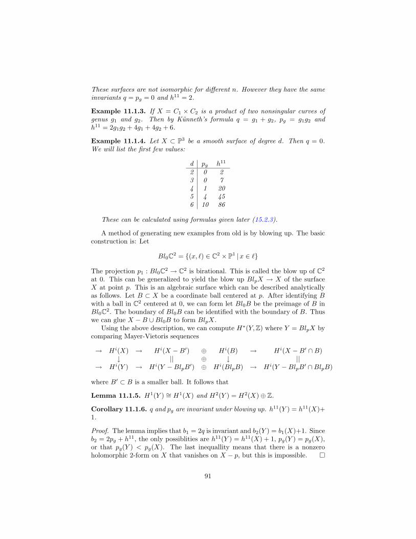
These surfaces are not isomorphic for different n. However they have the sameinvariants q = pg = 0 and h11 = 2.
Example 11.1.3. If X = C1 × C2 is a product of two nonsingular curves ofgenus g1 and g2. Then by Kunneth’s formula q = g1 + g2, pg = g1g2 andh11 = 2g1g2 + 4g1 + 4g2 + 6.
Example 11.1.4. Let X ⊂ P3 be a smooth surface of degree d. Then q = 0.We will list the first few values:
d pg h11
2 0 23 0 74 1 205 4 456 10 86
These can be calculated using formulas given later (15.2.3).
A method of generating new examples from old is by blowing up. The basicconstruction is: Let
Bl0C2 = (x, `) ∈ C2 × P1 |x ∈ `
The projection p1 : Bl0C2 → C2 is birational. This is called the blow up of C2
at 0. This can be generalized to yield the blow up BlpX → X of the surfaceX at point p. This is an algebraic surface which can be described analyticallyas follows. Let B ⊂ X be a coordinate ball centered at p. After identifying Bwith a ball in C2 centered at 0, we can form let Bl0B be the preimage of B inBl0C2. The boundary of Bl0B can be identified with the boundary of B. Thuswe can glue X −B ∪Bl0B to form BlpX.
Using the above description, we can compute H∗(Y, Z) where Y = BlpX bycomparing Mayer-Vietoris sequences
→ Hi(X) → Hi(X −B′) ⊕ Hi(B) → Hi(X −B′ ∩B)↓ || ⊕ ↓ ||
→ Hi(Y ) → Hi(Y −BlpB′) ⊕ Hi(BlpB) → Hi(Y −BlpB
′ ∩BlpB)
where B′ ⊂ B is a smaller ball. It follows that
Lemma 11.1.5. H1(Y ) ∼= H1(X) and H2(Y ) = H2(X)⊕ Z.
Corollary 11.1.6. q and pg are invariant under blowing up. h11(Y ) = h11(X)+1.
Proof. The lemma implies that b1 = 2q is invariant and b2(Y ) = b1(X)+1. Sinceb2 = 2pg + h11, the only possiblities are h11(Y ) = h11(X) + 1, pg(Y ) = pg(X),or that pg(Y ) < pg(X). The last inequallity means that there is a nonzeroholomorphic 2-form on X that vanishes on X − p, but this is impossible.
91
A morphism of varieties f : V →W is called birational if it is an isomorphismwhen restricted to nonempty Zariski open sets of X and Y . A birational mapV 99K W is simply an isomorphism of Zariski open sets. Blow ups and theirinverses (“blow downs”) are examples of birational morphisms and maps. Forthe record, we point out
Theorem 11.1.7 (Castelnuovo). Any birational map between algebraic sur-faces is a given by a finite sequence of blow ups and downs.
Therefore, we get the birational invariance of q and pg. However, there areeasier ways to prove this. Blow ups can also be used to extend meromorphicfunctions. A meromorphic function f : X 99K P1 is a holomorphic map from anopen subset U ⊆ P1 which can be expressed locally as a ratio of holomorphicfunctions.
Theorem 11.1.8 (Zariski). If f : X 99K P1 meromorphic function on analgebraic surface. Then there is a finite sequence of blow ups such that Y → Xsuch that f extends to a holomorphic map f ′ : X → P1.
Exercise 11.1.9.
1. Compare the construction of the blow up given here and in section 2.4(identify ((x, t) with ((x, xt), [t, 1])).
2. Finish the proof of lemma 11.1.5.
11.2 Castenuovo-de Franchis’ theorem
When can try to study varieties by mapping them onto lower dimensional va-rieties. In the case of surfaces, the target should be a curve. A very usefulcriterion for this is
Theorem 11.2.1 (Castenuovo-de Franchis). Suppose X is an algebraic sur-face. A necessary and sufficient condition for X to admit a constant holomor-phic map to a smooth curve of genus g ≥ 2 is that there exists two linearindependant forms ωi ∈ H0(X, Ω1
X) such that ω1 ∧ ω2 = 0.
The necessity is clear. We will sketch part of the argument of the converse,since it gives a nice application of corollary 10.2.6. A complete proof can befound in [BPV, pp123-125]. Choosing local coordinates, we can write
ωi = fi(z1, z2)dz1 + gi(z1, z2)dz2
The condtion ω1 ∧ ω2 = 0 is
(f1g2 − f2g1)dz1 ∧ dz2 = 0
which implies thatf2/f1 = g2/g1.
92
Thus ω2 = F (z1, z2)ω1. Since ωi are globally defined, F = ω2/ω1 defines aglobal meromorphic function X 99K P1. Since ωi are closed (corollary 10.2.6),
dF ∧ ω1 = dω2 = 0 (11.1)
Choose a “general” point p ∈ X and let t1 be a local coordinate centered atF (p). Let us also use t1 for the pullback of this function to neighbbourhood ofp. Then we can choose a function t2 such that t1, t2 give local coordinates atp. (11.1) becomes dt1 ∧ ω1 = 0. Consequently ω1 = f(t1, t2)dt1. The relationdω1 = 0, implies f is a function of t1 alone. Thus ω1 is locally the pullback ofa 1-form on P1, and likewise for ω2. This not true globally, since in fact thereare no nonzero holomorphic 1-forms on P1. What we can do is the following.By theorem 11.1.8, there exists a blow up Y → X such that F extends to aholomorphic function F ′ : Y → P1. The fibers of F ′ will not be connected. Atheorem of Stein shows that the map can be factored as Y → C → P1, wherethe first map has connected fibers and C → P1 is a finite to one map of curves.The argument above can be used to show that ωi are pullback from holomorphic1-forms on C. The final step is to prove that, the blow up is unnecessary, i.e.we can take Y = X.
An obvious corollary is:
Corollary 11.2.2. If q ≥ 2 and pg = 0, then X admits a constant map to acurve as above.
This can be improved substatially [BPV, IV, 4.2].
11.3 The Neron-Severi group
Let X be an algebraic surface once again. The image of the first Chern classmap is the Neron-Severi group NS(X) = H2(X, Z)∩H11(X). The rank of thisgroup is called Picard number ρ(X). We have ρ ≤ h11 with equality if pg = 0.
A divisor on X is a finite integer linear combination∑
niDi of possiblysingular curves Di. We can define a line bundle OX(D) as we did for Riemannsurfaces in section 5.5. If fi are local equations of Di ∩ U in some open set U ,
OX(D)(U) = OX(U)1
fn11 fn2
2 . . .
is a fractional ideal.
Proposition 11.3.1. If D is a smooth curve, then c1(OX(D)) = [D].
The cup product pairing
H2(X, Z)×H2(X, Z)→ H4(X, Z)→ Z
restricts to NS(X) denoted by “·”.
93
Lemma 11.3.2. Given a pair of transverse smooth curves D and E,
D · E =∫
X
c1(O(D)) ∪ c1(O(E)) = #(D ∩ E)
Proof. This follows from the propositions 11.3.1 and 4.4.2. The number ip(D,E)is seen to be always +1 in this case.
If the intersection of the curves D and E is finite but not transverse, it is stillpossible to give a geometric meaning to the above product. For each p ∈ X, letOan
p and Op be the rings of germs of holomorphic respectively regular functionsat p. Let f, g ∈ Op ⊂ Oan
p be the local equations of D and E respectively.Define ip(D,E) = dimOp/(f, g). Then
Lemma 11.3.3.
ip(D,E) = dimOanp /(f, g) =
1(2π√−1)2
∫|f(z)|=|g(z)|=ε
df ∧ dg
fg
Proof. [GH, pp. 662-670].
Proposition 11.3.4. If D,E are smooth curves such D ∩ E is finite, then
D · E =∑p∈X
ip(D,E)
Recall that H2(P2, Z) = H4(P2, Z) = Z, and the generator of H2(P2, Z) isthe class of line [L]. Given a curve D defined by a polynomial f , we definedeg D = deg f . Then [D] = deg D[L].
Corollary 11.3.5 (Bezout). If D,E are smooth curves on P2 with a finiteintersection, ∑
p∈X
ip(D,E) = deg(D) deg(E)
Proof. We have [D] = deg D[L], and [E] = deg E[L], so that D·E = deg D deg EL·L = deg D deg E.
Exercise 11.3.6.
1. Let X = C × C be product of a curve with itself. Consider, the divisorsH = C × p, V = p × C and the diagonal ∆. Show that these areindependent in NS(X)⊗Q.
2. E = C/(Z + Zτ) be an elliptic curve, and let X = E × E. Calculate thePicard number, and show that it could be 3 or 4 depending on τ .
94
11.4 The Hodge index theorem
Let X a compact Kahler surface. Then the Kahler for ω is closed real (1, 1)form, therefore it defines an element of H11(X) ∩H2(X, R).
Theorem 11.4.1. Let X be a compact Kahler surface. Then the restriction ofthe cup product to (H11(X) ∩H2(X, R)) ∩ (R[ω])⊥ is negative definite.
Proof. Locally, we can find an orthonormal basis φ1, φ2 of E(1,0). In this basis,
ω =√−12
(φ1 ∧ φ1 + φ2 ∧ φ2)
and the volume form
dvol =ω2
2=
(2√−1
)2
φ1 ∧ φ1 ∧ φ2 ∧ φ2
Choose an element of (H11(X)∩H2(X, R))∩ (R[ω])⊥ and represent it by a real(1, 1) form
α =∑
aijφi ∧ φj
Since α = α, aji = aij .∫X
α ∧ ω =2√−1
∫X
(a11 + a22)dvol = 0.
which shows a11 + a22 = 0. Therefore∫X
α ∧ α = 2(
2√−1
)2 ∫X
(|a11|2 + |a12|2)dvol < 0
Let X be a smooth projective surface. A divisor H on X is called if calledvery ample if there is an embedding X ⊂ Pn such that OX(H) ∼= OPn(1)|X .H is ample if some positive multiple is very ample. Since H2(Pn, C) is onedimensional, the cohomology class associated to the Kahler class ω of the Fubini-Study metric 9.1.3. would have to be a nonzero multiple of c1(O(1)). In fact,the constants in ω are chosen so that these coincide. Thus [H] = c1(O(H)) willbe the Kahler class for the induced metric, when H is very ample.
Corollary 11.4.2. If H is an ample divisor on an algebraic surface, the inter-section pairing is negative definite on (NS(X)⊗ R) ∩ (RH)⊥
If H is ample, then H2 > 0. The converse is false. Therefore when the cupproduct form is diagonalized, the diagonal consists of one 1 followed by ρ − 1−1’s. So we obtain
Corollary 11.4.3. If H,D are divisors on an algebraic surface such that H2 >0 and D ·H = 0, then D2 < 0
95
Exercise 11.4.4.
1. Prove that the restriction of the cup product to (H20(X) + H02(X)) ∩H2(X, R) is positive definite.
2. Conclude that (the matrix representing) the cup product pairing has 2pg+1positive eigenvalues. Therefore pg is a topological invariant.
96
Chapter 12
Topology of families
12.1 Fiber bundles
A C∞ map f : X → Y of manifolds is called a fiber bundle if it is locally aproduct of Y with another manifold (called the fiber). It is called trivial if f isa product. Nontrivial bundles over S1 can be constructed as follows. Let F bea manifold with a diffeomorphism φ : F → F , then glue F ×0 in F × [0, 1] toF × 1 by identifying (x, 0) to (φ(x), 1). This includes the familiar example ofthe Mobius strip where F = R and φ is multiplication by −1. If the induced mapφ∗ : H∗(F )→ H∗(F ), called monodromy, is nontrivial then the fiber bundle isnontrivial.
A C∞ map f : X → Y is called a submersion if the map on tangent spacesis surjective. The fibers of such a map are submanifolds. A continuous map oftopological spaces is called proper if the preimage of any compact set is compact.
Theorem 12.1.1 (Ehresmann). Let f : X → Y be a proper smooth map ofC∞ connected manifolds. Then f is a C∞ fiber bundle; in particular, the fibersare diffeomorphic.
Proof. A complete proof can be found in [MK, 4.1]. Here we sketch the proofof the last statement. Since Y is connected, we can join any two points, say0 and 1 by a path. Thus we replace Y by an interval, and hence by R whichis diffeomorphic to it. Choose a Riemmanian metric on X, then by the innerproducts allow us to define a vector field (the gradient) ∇f dual to the differ-ential df . By assumption df and therefore ∇f is nowhere zero. The existenceand uniqueness theorem of ordinary linear differential equations allows us todefine, for each p ∈ f−1(0), a C∞ path γp : R → X passing through p at time0 and with velocity ∇f . Then the gradient flow p 7→ γp(1) gives the desireddiffeomorphism.
97
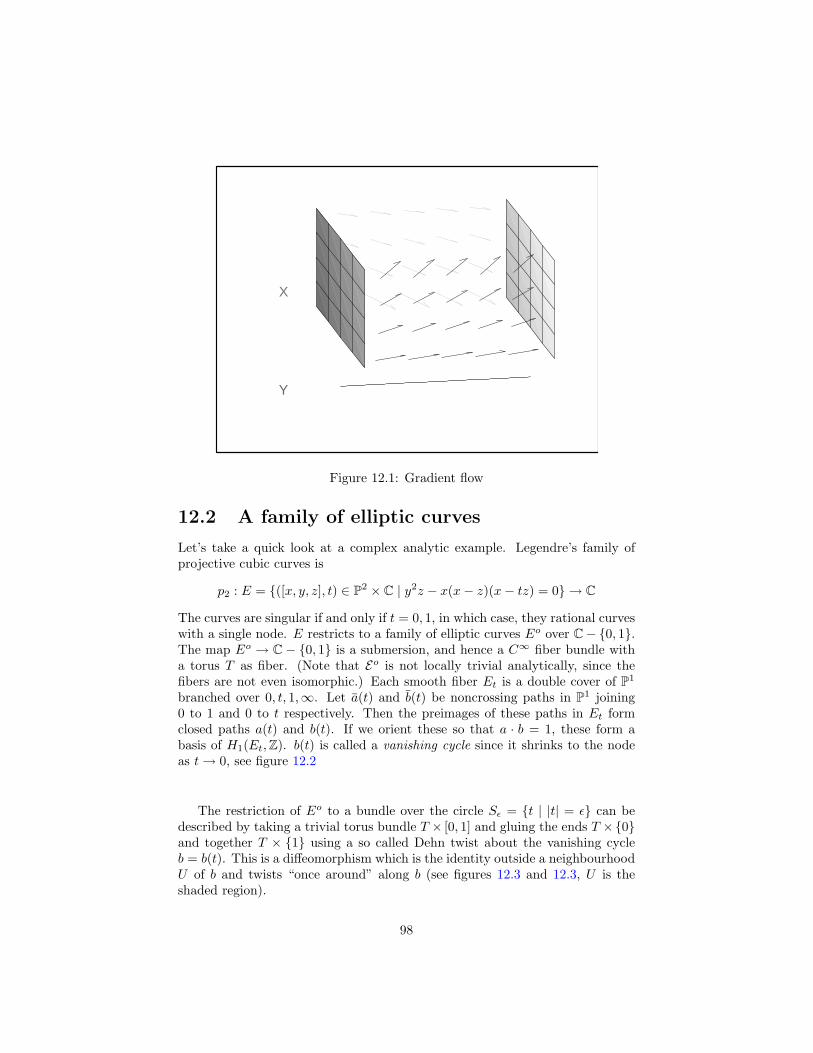
Y
X
Figure 12.1: Gradient flow
12.2 A family of elliptic curves
Let’s take a quick look at a complex analytic example. Legendre’s family ofprojective cubic curves is
p2 : E = ([x, y, z], t) ∈ P2 × C | y2z − x(x− z)(x− tz) = 0 → C
The curves are singular if and only if t = 0, 1, in which case, they rational curveswith a single node. E restricts to a family of elliptic curves Eo over C− 0, 1.The map Eo → C − 0, 1 is a submersion, and hence a C∞ fiber bundle witha torus T as fiber. (Note that Eo is not locally trivial analytically, since thefibers are not even isomorphic.) Each smooth fiber Et is a double cover of P1
branched over 0, t, 1,∞. Let a(t) and b(t) be noncrossing paths in P1 joining0 to 1 and 0 to t respectively. Then the preimages of these paths in Et formclosed paths a(t) and b(t). If we orient these so that a · b = 1, these form abasis of H1(Et, Z). b(t) is called a vanishing cycle since it shrinks to the nodeas t→ 0, see figure 12.2
The restriction of Eo to a bundle over the circle Sε = t | |t| = ε can bedescribed by taking a trivial torus bundle T × [0, 1] and gluing the ends T ×0and together T × 1 using a so called Dehn twist about the vanishing cycleb = b(t). This is a diffeomorphism which is the identity outside a neighbourhoodU of b and twists “once around” along b (see figures 12.3 and 12.3, U is theshaded region).
98
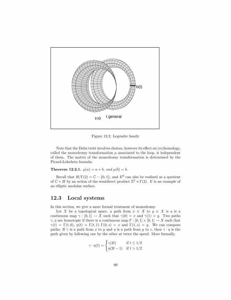
t=0 t general
b(t)
Figure 12.2: Legendre family
Note that the Dehn twist involves choices, however its effect on (co)homology,called the monodromy transformation µ associated to the loop, is independentof them. The matrix of the monodromy transformation is determined by thePicard-Lefschetz formula:
Theorem 12.2.1. µ(a) = a + b, and µ(b) = b.
Recall that H/Γ(2) = C− 0, 1, and E0 can also be realized as a quotientof C×H by an action of the semidirect product Z2 o Γ(2). E is an example ofan elliptic modular surface.
12.3 Local systems
In this section, we give a more formal treatment of monodromy.Let X be a topological space, a path from x ∈ X to y ∈ X is a is a
continuous map γ : [0, 1] → X such that γ(0) = x and γ(1) = y. Two pathsγ, η are homotopic if there is a continuous map Γ : [0, 1]× [0, 1]→ X such thatγ(t) = Γ(t, 0), η(t) = Γ(t, 1) Γ(0, s) = x and Γ(1, s) = y. We can composepaths: If γ is a path from x to y and η is a path from y to z, then γ · η is thepath given by following one by the other at twice the speed. More formally,
γ · η(t) =
γ(2t) if t ≤ 1/2η(2t− 1) if t > 1/2
99
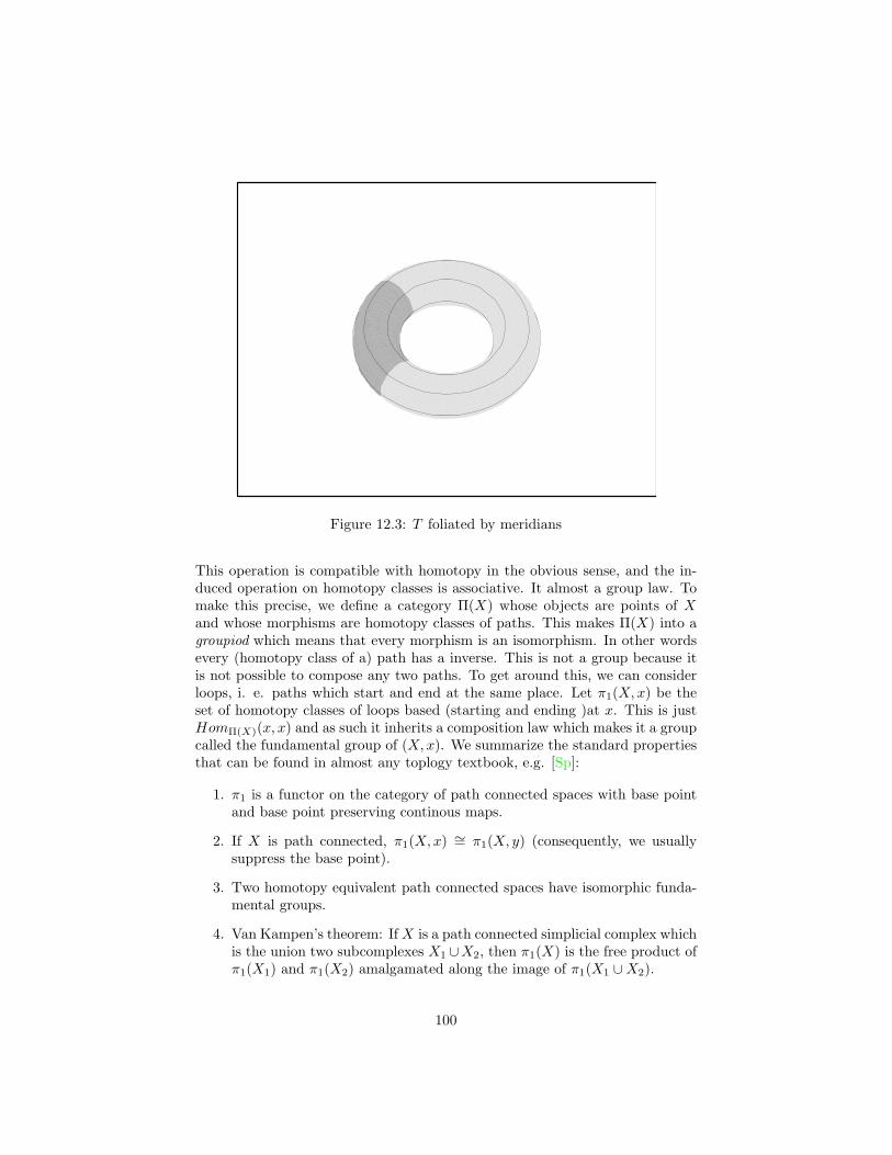
Figure 12.3: T foliated by meridians
This operation is compatible with homotopy in the obvious sense, and the in-duced operation on homotopy classes is associative. It almost a group law. Tomake this precise, we define a category Π(X) whose objects are points of Xand whose morphisms are homotopy classes of paths. This makes Π(X) into agroupiod which means that every morphism is an isomorphism. In other wordsevery (homotopy class of a) path has a inverse. This is not a group because itis not possible to compose any two paths. To get around this, we can considerloops, i. e. paths which start and end at the same place. Let π1(X, x) be theset of homotopy classes of loops based (starting and ending )at x. This is justHomΠ(X)(x, x) and as such it inherits a composition law which makes it a groupcalled the fundamental group of (X, x). We summarize the standard propertiesthat can be found in almost any toplogy textbook, e.g. [Sp]:
1. π1 is a functor on the category of path connected spaces with base pointand base point preserving continous maps.
2. If X is path connected, π1(X, x) ∼= π1(X, y) (consequently, we usuallysuppress the base point).
3. Two homotopy equivalent path connected spaces have isomorphic funda-mental groups.
4. Van Kampen’s theorem: If X is a path connected simplicial complex whichis the union two subcomplexes X1 ∪X2, then π1(X) is the free product ofπ1(X1) and π1(X2) amalgamated along the image of π1(X1 ∪X2).
100
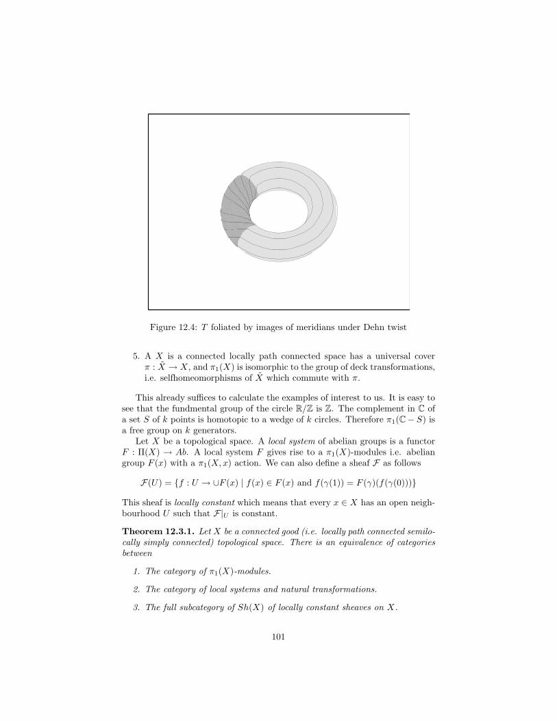
Figure 12.4: T foliated by images of meridians under Dehn twist
5. A X is a connected locally path connected space has a universal coverπ : X → X, and π1(X) is isomorphic to the group of deck transformations,i.e. selfhomeomorphisms of X which commute with π.
This already suffices to calculate the examples of interest to us. It is easy tosee that the fundmental group of the circle R/Z is Z. The complement in C ofa set S of k points is homotopic to a wedge of k circles. Therefore π1(C− S) isa free group on k generators.
Let X be a topological space. A local system of abelian groups is a functorF : Π(X) → Ab. A local system F gives rise to a π1(X)-modules i.e. abeliangroup F (x) with a π1(X, x) action. We can also define a sheaf F as follows
F(U) = f : U → ∪F (x) | f(x) ∈ F (x) and f(γ(1)) = F (γ)(f(γ(0)))
This sheaf is locally constant which means that every x ∈ X has an open neigh-bourhood U such that F|U is constant.
Theorem 12.3.1. Let X be a connected good (i.e. locally path connected semilo-cally simply connected) topological space. There is an equivalence of categoriesbetween
1. The category of π1(X)-modules.
2. The category of local systems and natural transformations.
3. The full subcategory of Sh(X) of locally constant sheaves on X.
101
In view of this theorem, we will treat local systems and locally constantsheaves as the same.
Let f : X → Y be a fiber bundle. We are going to construct a local systemwhich takes y → Hi(Xy, Z). Given a path γ : [0, 1] → Y joining y0 andy1, the pullback γ∗X = (x, t) | f(x) = γ(t) will be a trivial bundle over[0, 1]. Therefore γ∗X will be homotopic to both Xy0 and Xy1 , and so we haveisomorphisms
Hi(Xy0)∼← Hi(γ∗X) ∼→ Hi(Xy1)
The map Hi(Xy0)→ Hi(Xy1) can be seen to depend only on the homotopy classof the path, thus we have a local system which gives rise to a locally constantsheaf which will be constructed directly in the next section.
12.4 Higher direct images
Let us start with a rather general situation. Let f : X → Y be a continuous mapand F ∈ Sh(X) a sheaf. We can define the higher direct images by imitatingthe definition of Hi(X,F) in section 3.2.
R0f∗F = f∗FR1f∗F = coker[f∗G(F)→ f∗C
1(F)]Rn+1f∗F = R1f∗C
n(F)
Then we have an analogue of theorem 3.2.1.
Theorem 12.4.1. Given an exact sequence of sheaves
0→ A→ B → C → 0,
there is a long exact sequence
0→ R0f∗A→ R0f∗B → R0f∗C → R1f∗A . . .
There is an alternative description which is a bit more convenient.
Lemma 12.4.2. If f : X → Y is a continuous map, and F ∈ Sh(X), thenRif∗F(U) is the sheafification of U 7→ Hi(U,F)
Each element of Hi(X,F) determines an a global section of the presheaf U 7→Hi(U,F) and hence of the sheaf Rif∗F . This map Hi(X,F)→ H0(X, Rif∗F)is often called an edge homomorphism.
Let us now assume that f : X → Y is a fiber bundle of triangulable spaces.Then choosing a contractible neighbourhood U of y, we see that Hi(U, Z) ∼=Hi(Xy, Z). Since such neigbourhoods are cofinal, it follows that Rif∗Z is locallyconstant. This coincides with the sheaf associated to the local system Hi(Xy, Z)constructed in the previous section. The global sections of H0(Y, Rif∗Z) isthe space Hi(Xy, Z)π1(Y,y) of invariant cohomology classes on the fiber. Wecan construct elements of this space using the edge homomorphism. For more
102
general maps, we still have (Rif∗Z)y∼= Hi(Xy, Z), but the ranks can jump, so
these need not be locally constant.The importance of the higher direct images is that it allows the cohomology
of X to be computed on Y . The precise relationship is given by the Lerayspectral sequence
Epq2 = Hp(Y, Rqf∗F)⇒ Hp+q(X,F)
which we won’t go into. However, we will explain one of its consequences.
Proposition 12.4.3. If F is a sheaf of vector spaces over a field, such thatdim Hp(Y,Rqf∗F) <∞, then
dim Hi(X,F) ≤∑
p+q=i
Hp(Y, Rqf∗F)
It is possible to give a self contained proof of this using corollary 10.4.2.
Exercise 12.4.4.
1. Prove theorem 12.4.1.
103

Chapter 13
The Hard LefschetzTheorem
13.1 Hard Lefschetz and its consequences
Let X be an n dimensional compact Kahler manifold. Recall that L was definedby wedging with Kahler class ω. Since ω is closed, L takes closed (respectivelyexact) forms to closed ( exact) forms. Therefore this operation is defined oncohomology. The space
P i(X) = ker[Ln−i+1 : Hi(X, C)→ H2n−i+2(X, C)]
is called the primitive part of cohomology.
Theorem 13.1.1. For every i,
Li : Hn−i(X, C)→ Hn+i(X, C)
is an isomorphism. For every i,
Hi(X, C) =[i/2]⊕j=0
LjP i−2j(X)
We indicate the proof in the next section. As a simple corollary we findthat the Betti numbers bn−i = bn+i. Of course, this is nothing new since thisalso follows Poincare duality. However, it is easy to extract some less trivial“numerology”.
Corollary 13.1.2. The Betti numbers satisfy bi−2 ≤ bi for i ≤ n/2.
Proof. The theorem implies that the map L : Hi−2(X) → Hi(X) is injective.
104
Suppose that X = Pn with the Fubini-Study metric 9.1.3. the Kahler classω = c1(O(1)). The class c1(O(1))i 6= 0 is the fundamental class of a codimen-sion i linear space (see sections 6.2 and 6.5), so it is nonzero. Since all thecohomology groups of Pn are either 0 or 1 dimensional, this implies the HardLefschetz theorem for Pn. Things get much more interesting when X ⊂ Pn is anonsingular subvariety with induced metric. By Poinare duality and the previ-ous remarks, we get a statement closer to what Lefschetz would have stated1.Namely, that any element of Hn−i(X, Q) is homologous to the intersection of aclass in Hn+i(X, Q) with a codimension i subspace.
The Hodge index for surfaces admits the following generalization called theHodge-Riemman relations to an dimensional compact Kahler manifold X. Con-sider the pairing
Hi(X, C)×Hi(X, C)→ C
defined by
Q(α, β) = (−1)i(i−1)/2
∫X
α ∧ β ∧ ωn−i
Theorem 13.1.3. Hi(X) = ⊕Hpq(X) is an orthogonal decomposition. If α ∈P p+q(X) ∩Hpq(X) is nonzero,
√−1
p−qQ(α, α) > 0.
Proof. See [GH, p.123].
Let us introduce the Weil operator C : P i(X) → P i(X) which acts onP p+q(X) ∩Hpq(X) by multiplication by
√−1
p−q.
Corollary 13.1.4. The form Q(α, β) = Q(α, Cβ) on P i(X) is positive definiteHermitean.
13.2 More identities
Let X be as in the previous section. We defined the operators L,Λ acting formsE•(X) in section 9.1. We define a new operator H which acts by multiplicationby n− i on E i(X). Then:
Proposition 13.2.1. The following hold:
1. [Λ, L] = H
2. [H,L] = −2L
3. [H,Λ] = 2Λ
1Lefschetz stated a version of this theorem for varieties in his book [L], but to my knowledgeno one has ever made his proof rigorous. The first correct proof is due to Hodge usingharmonic forms. A subsequent arithemetic proof was given by Deligne. However, there is stillno geometric proof.
105

Furthermore these operators commute with ∆.
Proof. See [GH, p 115, 121].
This plus the following theorem of linear algebra will prove the Hard Lef-schetz theorem.
Theorem 13.2.2. Let V be a vector space with endomorphisms L, Λ,H satis-fying the above idenities. Then
1. H is diagonalizable with integer eigenvalues.
2. For each a ∈ Z let Va be the space of eigenvectors of H with eigenvalue a.Then Li induces an isomomorphism between Vi and V−i.
3. If P = ker(Λ), then
V = P ⊕ LP ⊕ L2P ⊕ . . .
4. α ∈ P ∩ Vi then Li+1α = 0.
We should say a few words about this mysterious theorem of linear algebra.Consider Lie algebra sl2(C) of space of traceless 2 × 2 complex matrices. Thisis a Lie algebra with a basis is given by
λ =(
0 10 0
)
` =(
0 01 0
)
h =(
1 00 −1
)These matrices satisfy
[λ, `] = h, [h, λ] = 2λ, [h, `] = −2`
So the hypothesis of the theorem is simply that V is a representation of sl2(C).The theorem can then be deduced from the following two facts from represen-tation theory of sl2(C) (which can be found in almost any book on Lie theory):
1. Every representation of sl2(C) is a direct sum of irreducible representa-tions.
2. An irreducible representation is classified by an integer N ≥ 0, and hasthe following structure
0 V−N = C` 6=0 //
λoo V−N+2 = C
λ6=0oo
` 6=0 // . . .λ6=0
oo` 6=0//
VN = Cλ6=0
oo` // 0
106
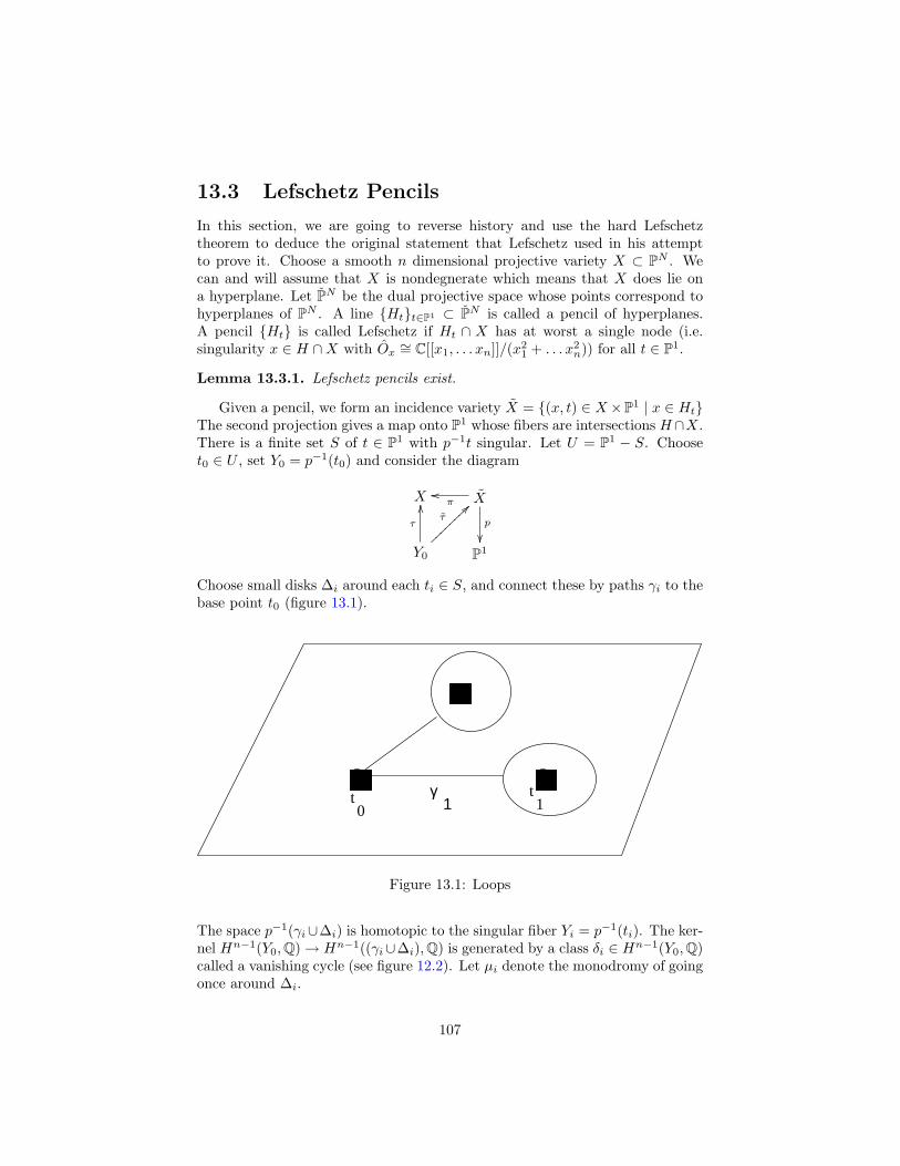
13.3 Lefschetz Pencils
In this section, we are going to reverse history and use the hard Lefschetztheorem to deduce the original statement that Lefschetz used in his attemptto prove it. Choose a smooth n dimensional projective variety X ⊂ PN . Wecan and will assume that X is nondegnerate which means that X does lie ona hyperplane. Let PN be the dual projective space whose points correspond tohyperplanes of PN . A line Htt∈P1 ⊂ PN is called a pencil of hyperplanes.A pencil Ht is called Lefschetz if Ht ∩ X has at worst a single node (i.e.singularity x ∈ H ∩X with Ox
∼= C[[x1, . . . xn]]/(x21 + . . . x2
n)) for all t ∈ P1.
Lemma 13.3.1. Lefschetz pencils exist.
Given a pencil, we form an incidence variety X = (x, t) ∈ X×P1 | x ∈ HtThe second projection gives a map onto P1 whose fibers are intersections H∩X.There is a finite set S of t ∈ P1 with p−1t singular. Let U = P1 − S. Chooset0 ∈ U , set Y0 = p−1(t0) and consider the diagram
X X
p
πoo
Y0
τ
OOτ
>>~~~~~~~~P1
Choose small disks ∆i around each ti ∈ S, and connect these by paths γi to thebase point t0 (figure 13.1).
t t0 1
γ1
Figure 13.1: Loops
The space p−1(γi∪∆i) is homotopic to the singular fiber Yi = p−1(ti). The ker-nel Hn−1(Y0, Q)→ Hn−1((γi∪∆i), Q) is generated by a class δi ∈ Hn−1(Y0, Q)called a vanishing cycle (see figure 12.2). Let µi denote the monodromy of goingonce around ∆i.
107
Theorem 13.3.2 (Picard-Lefschetz). µi(α) = α±〈α, δi〉δi where 〈, 〉 denotesthe cup product pairing on Hn−1(Y0, Q)
Proof. [La].
Let V ⊂ Hn−1(Y0, Q) be the subspace spanned by the δi.
Corollary 13.3.3. The orthogonal complement V ⊥ coincides with the subspaceHn−1(Y0)π1(U) ⊂ Hn−1(Y0) of classes invariant under π1(U).
The image of Hn−1(X, Q) lies in Hn−1(Y0)π1(U) since it factors throughHn−1(X, Q).
Theorem 13.3.4.
(a) V is an irreducible π1(U)-module.
(b) Hn−1(Y0)π1(U) = τ∗Hn−1(X, Q).
(c) τ∗Hn−1(X, Q) ∩ V = 0.
(d) Hn−1(Y, Q) = τ∗Hn−1(X, Q)⊕ V
Proof. We prove the last two statements. For the previous statements, see[La]. By Poincare duality dim Hn−1(Y, Q) = dim V + dim V ⊥. By part (b) andcorollary 13.3.3, τ∗Hn−1(X) = V ⊥. The restriction of the cup product pairingto τ∗Hn−1(X) coincides with the pairing
(α, β) 7→∫
Y
τ∗α ∪ τ∗β = ±Q(α, β)
which is nondegenerate by corollary 13.1.4. This implies that V ∩V ⊥ = 0 whichproves (c) and (d).
13.4 Barth’s theorem
Hartshorne [H1] gave a short elegent proof of a theorem of Barth based on thehard Lefschetz theorem. His reproduce his argument here.
Proposition 13.4.1. If X is an n dimensional nonsingular complex projectivevariety, such there positive integers m < n and N ≤ 2m− n for which
1 = b2 = b4 = . . . b2([N/2]+n−m)
b1 = b3 = . . . b1+2([(N−1)/2]+n−m)
Then if Y ⊂ X a nonsingular m dimensional subvariety, the restriction mapHi(X, Q)→ Hi(Y, Q) is an isomorphism for i < N .
108
Proof. The assumtions imply that H2(n−m)(X) is generated by Ln−m. There-fore [Y ] = d[H]n−m with d 6= 0. Let ι : Y → X denote the inclusion. Let L bethe Lefschetz operator associated to H and H|Y (it will be clear from context,which is which). Consider the diagram
Hi(X) Ln−m//
ι∗
Hi+2(n−m)(X)
ι∗
Hi(Y ) Ln−m
//
(1/d)ι!88ppppppppppp
Hi+2(n−m)(X)
The diagram commutes thanks to the identities
ι∗ι!α = i∗[Y ] ∪ α
ι!ι∗β = [Y ] ∪ β
ι∗(β ∪ γ) = ι∗β ∪ ι∗γ
Hard Lefschetz for X implies that Ln−m : Hi(Y ) → Hi+2(n−m)(Y ) is in-jective and hence an isomorphism by our assumptions. It follows that the re-striction ι∗ : Hi(X) → Hi(Y ) is injective. It’s enough to prove equality ofdimension. Hard Lefschetz for Y implies that Ln−m : Hi(Y )→ Hi+2(n−m)(Y )is injective. Therefore the same is true of ι!. Therefore
bi(X) ≤ bi(Y ) ≤ bi+2(n−m)(X) = bi(X)
Corollary 13.4.2 (Barth). If Y ⊂ Pn is a nonsingular, complex projectivevariety, then Hi(Pn, Q)→ Hi(Y, Q) is an isomorphism for i < dim Y .
When Y has codimension one, this is the Lefschetz hyperplane theorem (ormore acurately a special case of it).
13.5 Hodge conjecture
Let X be an n dimensional nonsingular complex projective variety. We definethe space of codimension p Hodge cycles on X to be
Hodgep(X) = H2p(X, Z) ∩Hpp(X)
Lemma 13.5.1. Given a nonsingular subvariety i : Y → X of codimension p,the fundamental class [Y ] ∈ Hodgep(X)
Proof. [Y ] corresponds under Poincare duality to the functional α 7→∫
Yα. If
α has type (a, b), then α|Y = 0 unless a = b = p. Therefore [Y ] has type (p, p)thanks to corollary 10.2.8. The class [Y ] is also integral, hence the lemma.
109
Even if Y has singularities, a fundamental class can be defined with theabove properties. Here we give a quick but nonelementary definition. Let usfirst observe.
Lemma 13.5.2. α ∈ Hodgep(X) if and only if 1 7→ α defines a morphism ofHodge structures Z→ H2p(X, Z)(p). Consequently, Hodgep(X) ∼= Hom(Z,H2p(X, Z)(p)).
By Hironaka’s famous theorem [Ha], there exists a smooth projective varietyY with a birational map p : Y → Y . Let i : Y → X denote the composition ofp and the inclusion. By corollary 10.2.10, we have a morphism
i! : H0(Y ) = Z→∈ H2p(X)(−p)
This defines a class [Y ] ∈ Hodgep(X) which is easily seen to be independent ofY .
Let Ap(X) ⊆ Hodgep(X) ⊗ Q be the subspace spanned by fundamentalclasses of codimension p subvarieties. The (in)famous Hodge conjecture asserts:
Conjecture 13.5.3 (Hodge). Ap(X) and Hodgep(X)⊗Q coincide.
Note that in the original formulation Z was used in place of Q, but this isknown to be false [AH]. For p = 1, the conjecture is true by the Lefschetz (1, 1)theorem 9.3.1. We prove it holds for p = dim, X − 1.
Proposition 13.5.4. If the Hodge conjecture holds for X in degree p withp < n = dim X, i.e. if Ap(X) = Hodgep(X)⊗Q, then it holds in degree n− p.
Proof. Let L be the Lefshetz operator corresponding to a projective embeddingX ⊂ PN . Then for any subvariety Y L[Y ] = [Y ∩H] where H is a hyperplanesection chosen in general position. It follows thatLn−2p takes Ap(X) to An−p(X)and the map is injective. Thus
dim Hodgep(X)⊗Q = dim Ap(X) ≤ dim An−p(X) ≤ dim Hodgen−p(X)⊗Q
On the other hand Ln−2p induces an isomorphism of Hodge structures H2p(X, Q)(p−n) ∼= H2n−2p(X, Q), and therefore an isomorphism Hodgep(X)⊗Q ∼= Hodgen−p(X⊗Q). Thus forces equality of the above dimensions.
Corollary 13.5.5. The Hodge conjecture holds in degree n− 1.
Further information can be found in [Lw].
13.6 Degeneration of Leray
We want to mention one last consequence of the Hard Lefschetz theorem due toDeligne [D1]. A projective morphism of smooth complex algebraic varieties iscalled smooth if the induced maps on (algbraic) tangent spaces are surjective.In particular, such maps are C∞ fiber bundles.
110
Theorem 13.6.1. Let f : X → Y be smooth projective map of smooth complexalgberaic varieties, then the inequalities in proposition 12.4.3 for F = Q areequalities, i.e.
dim Hi(X, Q) =∑
p+q=i
Hp(Y, Rqf∗Q)
Note that this generally fails for C∞ fiber bundles.
111
Chapter 14
Coherent sheaves onProjective Space
In this chapter, we develop some algebraic tools for studying sheaves on projec-tive spaces. In the last section, we discuss Serre’s GAGA theorems which showsthat on projective varieties there is an equivalence between the algebraic andanalytic theories.
14.1 Cohomology of line bundles on Pn
Let k be a field, and let (Pnk ,OP) denote projective space over k viewed as an
algebraic variety 1.3 (even if k = C). Then Pnk has a covering by n + 1 open
affine sets Ui = xi 6= 0, where xi are the homogenous coordinates. Ui can beidentified with affine n-space with coordinates
x0
xi, . . .
xi
xi. . .
xn
xi
Our goal is to compute cohomology of OPn(i) using the Cech complex withrespect to this covering. But we need to show that this a Leray covering. Sincethe interesction of a finite number of the Ui’s is affine, this will follow from:
Theorem 14.1.1 (Serre). If X is an affine variety, then
Hi(X,OX) = 0
for all i > 0.
This will be proven in a more general form in section 16.2.
Theorem 14.1.2 (Serre). Let Si be the space of homogeneous degree i poly-nomials in the variables x0, . . . xn, then
a) H0(Pn,OP(d)) ∼= Sd (in particular it is 0 if d < 0).
112

b) Hi(Pn,OP(d)) = 0 if 0 6= i 6= n.
c) Hn(Pn,OP(d)) ∼= S−d−n−1.
A complete proof can be found in [H, III.5], although from a somewhat moregeneral point of view. We use Cech cohomology with respect to the coveringUi. We use the description of O(d) given in section 6.3, where we identify asection of O(d)(U) with collection of functions fi ∈ O(U ∩ Ui) satisfying
fi = (xj/xi)dfj
Formally cross multiplying yields
xdi fi = xd
jfj (14.1)
which will be more convenient for us. In order, to interpret this step, noteO(Ui) can be identified with the polynomial ring k[x0/xi, . . . xn/xi]. Let S =k[x0, . . . xn]. The localization
S
[1xi
]=
⊕d
S
[1xi
]d
has a natural Z-grading, where
S
[1xi
]d
=∑
e
Sd+e
xei
.
Similar statements apply to the other localizations S[1/xixj . . .] along mono-mials. Note the that degree 0 piece is exactly O(Ui). The sections φi = xd
i fi
should be viewed as elements of S[1/xi]d. At this point, we may well identifyO(d)(Ui) = S[1/xi]d, equation 14.1 then simply becomes φ = φj .
In general, the Cech complex for O(d) is the degree d piece of the complex⊕S
[1xi
]→
⊕S
[1
xixj
]→ . . .
where the maps are as defined alternating sums of the natural maps along thelines of section 6.3.
Notice that Hi(Pn,O(d)) is automatically zero when i > n because the Cechcomplex has length n, this takes care of part of (b). An element of H0(Pn,O(d))can be represented by a triple (p0/xe
0, p1/xe1, . . .) of rational expressions of degree
d, where the p’s are polynomials, satisfying
p0
xe0
=p1
xe1
=p2
xe2
. . .
This forces the polynomials pi to be divisible by xei . Thus the H0(Pn,O(d)) can
be identified with Sd as claimed in (a).
113
Hn(Pn,O(d)) is S[ 1x0...xn
] modulo the the space of coboundaries B, i. e. theimage of the previous term. S[ 1
x0...xn] is spanned by monomials xi0
0 . . . xinn with
arbitrary integer exponents. The image B is the space spanned by those mono-mials where at least one of the exponents is nonnegative. Therefore the quotientcan be identified with the complementary submodule spanned by monomialswith negative exponents. In particular
Hn(Pn,O(d)) ∼=⊕
i0+...in=d;i1,...in<0
kxi00 . . . xin
n .
This is isomorphic to S−d−n−1 via
xi00 . . . xin
n 7→ x−i0−10 . . . x−in−1
n
This proves (c).It remains to finish the proof (b). The reader can look up the argument in
[H, pp 227-228]. We will be content to work this out in for n = 2. This amountto the assertion that H1(P2,O(d)) vanishes. Our treatment will be elementarybut a little messy. A 1-cocycle is given by a triple pij/(xixj)k of rationalexpressions satisfying
p02
(x0x2)k=
p01
(x0x1)k+
p12
(x1x2)k.
We have to find polynomials qi satisfying
pij
(xixj)k=
qi
xki
− qj
xkj
.
The above relation is equivalent to
xk1p02 = xk
2p01 + xk0p12,
which implies p02 ∈ (xk0 , xk
2) and similarly p01 ∈ (xk0 , xk
1) and p12 ∈ (xk1 , xk
2).Therefore, we can find polynomials such that
p01 = xk1q0 − xk
0q1
p12 = xk2q′1 − xk
1q′2
Substituting back into the above relation shows that q1 − q′1 = xk1s for some
polynomial s. Now setting q2 = q′2 + s should work.
14.2 Coherence in general
Let (X,R) be a ringed space. We need to isolate a class of R-modules withgood finiteness properties.
Definition 14.2.1. Given a ringed space (X,R), an R-module E is coherent if
114
1. E is locally finitely generated, i. e., each point has a neighbourhood U suchthat R|nU surjects onto E|U for some n <∞.
2. If R|nU → E|U is a surjection, the kernel is finitely generated.
This definition has been given for completeness. We are really only inter-ested in certain standard examples. Standard properties of coherent sheaves onringed spaces can be found in [EGA] (the definition given in [H] is only validfor noetherian schemes).
Example 14.2.2. If M is a finitely generated module over a noetherian ringR, then M is coherent on SpecR.
Theorem 14.2.3 (Oka). If (X,OX) is a complex manifold, then OX is coher-ent.
Corollary 14.2.4. Any locally free OX-module is coherent.
In the next section, we will describe all coherent sheaves on projective space.
14.3 Coherent Sheaves on Pn
Let us revert to the notation of section 14.1. The ring S = k[x0, . . . xn] = ⊕Si
is graded, where Si is the space of homogenous polynomials of degree i. Let
S(j) = k
[x0
xj, . . .
xn
xj
]We can identify Spec S(j) with the affine space Uj = xj 6= 0.
Let M = ⊕Mi be a (finitely generated) graded S-module (in additional tobeing an S-module it satisfies SiMj ⊂Mi+j). Then
M(j) =∑
i
Mi[1xi
j
] ⊂M [1xi
j
]
is naturally a (finitely generated) Sj)-module. We can construct sheaves OUj-
modules M(j) as in section 2.5. These can be glued toegether:
Proposition 14.3.1. There exist an OPn-module M such that M |Uj∼= M(j).
The functor M → M from graded S-modules to OPn-modules is exact.
Proof. See [H, II, 5.11] for the first statement. Since exactness is a local property,the second statement follows from lemma 2.5.2.
It follows from this that M is coherent for any finitely generated gradedS-module M . Conversely:
Proposition 14.3.2. Any coherent sheaf on Pn is isomorphic to M for somefinitely generated graded S-module M .
115
Proof. [H, II, ex. 5.9]
Example 14.3.3. Let S(i) denote S with the shifted grading (S(i))j = Sj+i.Then O(i) = S(i). In particular, it is coherent.
Example 14.3.4. Let X ⊂ Pn be a closed subvariety and let IX be the homoge-nous ideal generated by homogenous polynomials vanishing along X. Then I isthe ideal sheaf IX , example 2.2.5.
As a corollary of proposition 14.3.1, we get
Corollary 14.3.5. The class of coherent sheaves is closed under kernels, cok-ernels and extensions.
It is possible to the impression that M 7→ M is one to one. But this is wrongas the following example shows.
Example 14.3.6. Let M be a graded module which is finite dimensional overk, so Mi = for i >> 0. Then M = 0.
If one “mods out” the above modules, then one does get an equivalence ofcategories. However, we won’t try to make this precise.
Any vector bundle is coherent, although this is far from clear with our defini-tion. For standard vector bundles, this can be checked directly using the abovecorollary.
Example 14.3.7. The tangent sheaf fits into an exact sequence
0→ OPn
x0
x1
. . .
−→ OPn(1)n+1 → TPn → 0
If we pull this back via π : An+1 − 0 → Pn, we can identitfy the second mapwith the derivative TAn−0 → π∗TPn , and the first map sends 1 to the Eulervector field
∑xi
∂∂xi
The Hilbert syzygy theorem [E, 1.13] says that any finitely generated gradedS-module has a finite graded resolution of length at most n. This immediatelygives:
Theorem 14.3.8. Any coherent sheaf E on Pn fits into an exact sequence
0→ Er → En−1 → . . . E0 → E → 0
where r ≤ n and each Ei is a sum of a finite number of line bundles OPn(j).
Theorem 14.3.9. If E is a coherent sheaf on Pn, then Hi(Pn, E) is finite di-mensional for each i, and is zero for i > n.
116
Proof. We prove this by induction on r, where r is the length of the shortestresolution given by theorem 14.3.8. If r = 0, we are done by theorem 14.1.2.Suppose, we know the theorem for all r′ < r. Choose a resolution
0→ Er → En−1 → . . . E0 → E → 0
and let E ′ = ker[E0 → E ]. We have exact sequences
0→ Er → En−1 → . . . E1 → E ′ → 0
and0→ E ′ → E0 → E → 0
The first sequence implies that H∗(Pn, E ′) is finite dimensional by the inductionhypothesis. The second sequences yields a long exact sequence
. . .Hi(Pn, E0)→ Hi(Pn, E)→ Hi+1(Pn, E ′) . . .
which finishes the proof. The vanishing for i > n can be proved by induction insimilar manner. Details are left as exercise.
Exercise 14.3.10.
1. Let f be a homogeneous polynomial of degree d in S = k[x0, x1, x2]. Thencorresponding to the exact sequence of graded modules
0→ S(−d) ∼= Sf → S → S/(f)→ 0
there is an exact sequence of sheaves
0→ OP2(−d)→ OP2 → OX → 0.
Prove that
dimH1(X,OX) =(d− 1)(d− 2)
2
2. Let f be a homogeneous polynomial of degree d in 4 variables. Repeat theabove for the first and second cohomology groups.
3. Prove the last part of theorem 14.3.9.
14.4 Hilbert Polynomial
The Euler characteristic of a sheaf F on a space X is
χ(F) =∑
(−1)i dim Hi(X,F)
provided that the sum is finite. The advantage of working with the Euler char-acteristic is the following:
117
Lemma 14.4.1. If0→ F1 → F2 → F3 → 0
is an exact sequence,χ(F2) = χ(F1) + χ(F3)
Given a coherent sheaf, E on Pn, let E(i) = E ⊗O(i). This is again coherent.If E = M for a finitely generated graded S-module M , then E(i) = M(i), whereM(i) denote M with grading shifted by i. A corollary of theorem 14.3.8 is:
Theorem 14.4.2. If E is a coherent sheaf on Pn, then i → χ(E(i)) is a poly-nomial in i. If X is a subvariety of Pn
k and E = OX , then this polynomial hasdegree dim X.
Proof. From theorem 14.1.2,
χ(OPn(i)) =
dim Si if i ≥ 0(−1)n dim S−d−n−1 otherwise
=(
n + i
n
),
which is a polynomial of degree n. This implies that χ(E(i)) is degree n polyno-mial when E is sum of line bundles OPn(j). In general, theorem 14.3.8 impliesthat for any coherent E
χ(E(i)) =r∑
j=0
(−1)jχ(Ej(i))
where Ej are sums of line bundles. This shows χ(E(i)) is degree n polynomialin general.
For the second, we use induction on dim X and the relation
χ(OH∩X(i)) = χ(OX(i))− χ(OX(i− 1))
which follows from the sequence
0→ OX(−1)→ OX → OH∩X → 0,
where H is a general hyperplane.
χ(E(i)) is called the Hilbert polynomial of E . It has a elementary algebraicinterpretation
Corollary 14.4.3 (Hilbert). Let M be a finitely generated graded S-module,then for i >> 0, dim Mi is given by a polynomial, and this coincides with theHilbert polynomial χ(M(i)).
118
14.5 GAGA
Let k = C. Let (Pn,OP) denote complex projective space as an algebraic variety,and (Pn
an,OPan) projective space as a complex manifold. In other words, Pn
(resp. Pnan) is endowed with the Zariski (strong) topology and OPn (resp. OPn
an)
is the sheaf of algebraic (resp. holomorphic) functions. We have a morphism ofringed spaces
ι : (Pn,OP)→ (Pnan,OPan)
Given an OP-module E , define the OPan-module Ean = ι∗E . Ean is coherent if
E is.
Theorem 14.5.1 (Serre). If E is a coherent OPan-module, then there exists aunique coherent OP-module F such that E ∼= Fan. There is an isomorphism
Hi(Pn,F) ∼= Hi(Pnan, E)
The GAGA theorem can fail for nonprojective varieties. For example, H0(OCnan
)is the space of holomorphic functions on Cn which is much bigger than the spaceH0(OCn) of polynomials.
Let X ⊆ Pn be a nonsingular subvariety. Then the sheaf of algebraic p-forms Ωp
X can be viewed as a coherent OP-module. Then (ΩpX)an is the sheaf of
holomorphic p-forms. In particular, OanX is the sheaf of holomorphic functions
of the associated complex manifold Xan. Thus:
Corollary 14.5.2 (Chow). Every complex submanifold of Pn is a projectivealgebraic subvariety.
Corollary 14.5.3. dimHq(X, ΩpX) coincides with the Hodge number hpq of the
manifold Xan.
119
Chapter 15
Computation of someHodge numbers
The GAGA theorem 14.5.1 allows us compute Hodge numbers by working inthe algebraic setting. We look a few examples.
15.1 Hodge numbers of Pn
Let S = k[x0, . . . xn] be a polynomial ring over a field and P = Pnk for some field
k. The basic result (which is dual to 14.3.7) is:
Proposition 15.1.1. There is an exact sequence
0→ Ω1P → OP(−1)n+1 → OP → 0
Proof. Let F = Sn+1 be the free module of rank n + 1 with basis vectors ei.We define a map of graded modules F (−1)→ S by sending ei to xi. Let K bethe kernel. We have an exact sequence of graded modules
0→ K → F (−1)→ m→ 0
where m = (x0, . . . xn)....
Proposition 15.1.2. Given an exact sequence of locally free sheaves
0→ A→ B → C → 0
If A has rank one, then
0→ A⊗ ∧p−1C → ∧pB → ∧pC → 0
is exact for any p. If C has rank one, then
0→ ∧pC → ∧pB → ∧p−1A⊗ C → 0
is exact for any p.
120
Proof. See [H, II, 5.16].
Corollary 15.1.3. There is an exact sequence
0→ ΩpP → OP(−p)(
n+1p ) → Ωp−1
P → 0
Proof. This follows from the above proposition and proposition 15.1.1, togetherwith the isomorphism
∧p[OP(−1)n+1] ∼= OP(−p)(n+1
p )
This corollary can be understood from another point of view. Using thenotation introduced in the proof of proposition 15.1.1, we can extend the mapF (−1)→ m to an exact sequence
0→ [∧n+1F ](−n− 1) δ→ . . . [∧2F ](−2) δ→ F (−1) δ→ m→ 0 (15.1)
whereδ(ei1 ∧ . . . eip
) =∑
(−1)pxijei1 ∧ . . . eij
∧ . . . eip
This is the so called Koszul resolution [E, chap 17] which is one of the basicworkhorses of homological algebra. The associated sequence of sheaves is
0→ [∧n+1On+1P ](−n− 1)→ . . . [∧2On+1
P ](−2)→ [On+1P ](−1)→ OP → 0
If we break this up into short exact sequences, then we obtain exactly thesequences in corollary 15.1.3.
Proposition 15.1.4.
Hq(P,ΩpP) =
k if p = q ≤ n0 otherwise
When k = C, this gives a new proof of the formula for Betti numbers of Pn
given in section 6.2.
15.2 Hodge numbers of a hypersurface
We now let X ⊂ Pn be a nonsingular hypersurface defined a degree d polynomial.
Proposition 15.2.1. The restriction map
Hq(Pn,ΩpP)→ Hq(Xn,Ωp
X)
is an isomorphism when p + q < n− 1.
121
When k = C (which we assume for the remainder of this section), this propo-sition can be deduced from corollary 13.4.2, the canonical Hodge decomposition(10.2.4) and GAGA. As corollary, we can calculate many of the Hodge numbersof X.
Corollary 15.2.2. The Hodge numbers hpq(X) = δpq, where δpq is the Kro-necker symbol, when n− 1 6= p + q < 2n− 2.
Proof. For p+q < n−1, this follows from the above proposition and proposition15.1.4. For p + q > n− 1, this follows from GAGA and 9.2.3.
This leaves the middle Hodge numbers. For h0,n−1(X), this is equivalent tocomputing the Euler characteristic χ(OX). From the sequence
0→ OPn(−d)→ OPn → OX → 0
we obtain
χ(OX) =(
i + n
n
)−
(i + n− d
n
).
In general, the formulas can be given in terms of a generating function. Lethpq(d) denote the pqth Hodge number of smooth hypersurface of degree d inPp+q+1. Define the formal power series
H(d) =∑pq
(hpq(d)− δpq)xpyq
in x and y. Then:
Theorem 15.2.3 (Hirzebruch).
H(d) =1
(1 + x)(1 + y)
[(1 + x)d − (1 + y)d
(1 + y)dx− (1 + x)dy− 1
]Hirzebruch [Hh] deduces a slightly different identity from his general Riemman-
Roch theorem. The above form of the identity appears in [SGA7, exp X1].Similar formulas are available for complete intersections.
Exercise 15.2.4.
1. Show that the generating for h0,q obtained by setting x = 0 in H(d) iscorrect.
15.3 Machine computations
The formulas of the previous section are easily implemented on computer and arerather efficient to use when X is a hypersurface (or a complete intersection).There is, in principle, a method for computing Hodge numbers of a generalX ⊂ Pn given explicit equations for it. In rough outline, one can proceed asfollows:
122
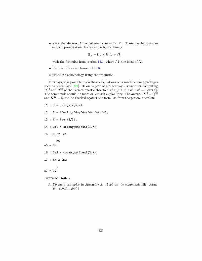
• View the sheaves ΩpX as coherent sheaves on Pn. These can be given an
explicit presentation. For example by combining
Ω1X = Ω1
Pn/(IΩ1Pn + dI),
with the formulas from section 15.1, where I is the ideal of X.
• Resolve this as in theorem 14.3.8.
• Calculate cohomology using the resolution.
Nowdays, it is possible to do these calculations on a machine using packagessuch as Macaulay2 [M2]. Below is part of a Macaulay 2 session for computingH12 and H22 of the Fermat quartic threefold x4 + y4 + z4 +u4 + v4 = 0 over Q.The commands should be more or less self explanitory. The answer H12 = Q30
and H22 = Q can be checked against the formulas from the previous section.
i1 : S = QQ[x,y,z,u,v];
i2 : I = ideal (x^4+y^4+z^4+u^4+v^4);
i3 : X = Proj(S/I);
i4 : Om1 = cotangentSheaf(1,X);
i5 : HH^2 Om1
30o5 = QQ
i6 : Om2 = cotangentSheaf(2,X);
i7 : HH^2 Om2
1o7 = QQ
Exercise 15.3.1.
1. Do more examples in Macaulay 2. (Look up the commands HH, cotan-gentSheaf... first.)
123

Chapter 16
Deformation invariance ofHodge numbers
In this chapter, the various strands (algebra, analysis, topology) will converge.Our goal is to prove that Hodge numbers of a family of smooth complex projec-tive varieties stays constant. While this can be proved purely analytically, wedevelop much of background using Grothendieck’s language of schemes whichgives a particularly elegant approach to families.
16.1 Families of varieties via schemes
We gave a definition of schemes 2.3 earlier without giving much geometric mo-tivation. Varieties often occur in families as we have already seen. As a simpleexample, let f(x, y, t) = y2−xt be a polynomial over a field k. We can view thisas defining a family of parabolas in the xy-plane A2 parameterized by t ∈ A1.When t = 0, we get a degenerate parabola y2 = 0 which is the “doubled” x-axis. It is impossible to capture this fully within the category of varieties, butit makes perfect sense with schemes. Here, we have a map of rings
k[t]→ k[x, y, t]/(f(x, y, t))
which induces a morphism of schemes
π : Spec k[x, y, t]/(f)→ Spec k[t] = A1
We can view this as the family of schemes
Spec k[x, y, t]/f(x, y, a) | a ∈ k
given by the fibers of π.More generally, let R = O(Y ) be the coordinate ring be an affine variety Y
over an algebraically closed field k. Affine space over R is
AnR = SpecR[x1, . . . xn] ∼= An
k × Y.
124
Let I ⊂ R[x1, . . . xn] be an ideal. It is generated by polynomials
fj(x, y) =∑
fj,i1,...in(y)xi1
1 . . . xinn .
We get a morphism
SpecR[x1, . . . xn]/I → SpecR = Y
We can view this as a family of affine subschemes of Ank
SpecR[x1, . . . xn]/I ⊗R/ma = Spec k[x1, . . . xn]/(fj(x, a))
parameterized by points a ∈ Y . If (fj(x, a)) is a radical ideal in k[x1, . . . xn],this would be a subvariety of An
k , but in general it be a closed subscheme.Similarly, a (not necessarily radical) homogenous ideal I ⊂ k[x1, . . . xn] gives
rise to a closed subscheme called Proj k[x1, . . . xn]/I of Pnk . More generally if
I ⊂ R[x1, . . . xn] = S is an ideal with homogenous generators fj(x, y). We canloosely define Proj S/I as the family of subschemes of Pn
k defined by the ideals(fj(x, a)) for points a ∈ Y . A bit more formally, the projective space over RPn
R = Pnk × Y can be constructed by gluing n + 1 copies of affine space
Ui,R = SpecR[x0/xi, . . . xi/xi . . . xn/xi]
together. Given a homogenous polynomial in f(x, y) ∈ S = R[x1, . . . xn], we geta polynomial in f(x1/xi, . . . xn/xi, y) in the above ring. Thus a homogenousideal I defines ideals in Ii ⊂ R[x1/xi, . . .] by applying this substitution on thegenerators. The scheme ProjS/I is defined by gluing the affine schemes definedIj together. See [H] for a more precise account of Proj.
16.2 Cohomology of Affine Schemes
Let R be a commutative ring.
Definition 16.2.1. An R-module I is injective iff for any for injective mapN → M of R-modules, the induced map HomR(M, I) → HomR(N, I) is sur-jective.
Example 16.2.2. If R = Z then I is injective provided that it is divisible i.e.if a = nb has a solution for every a ∈ I and n ∈ Z− 0.
A standard result of algebra is the following. A proof can be found in severalplaces, for example [E, p. 627].
Theorem 16.2.3 (Baer). Every module is (isomorphic to) a submodule of aninjective module.
Recall construction of the sheaf M of section 2.5.
Proposition 16.2.4. If I is injective and R is noetherian, then I is flabby.
125
Proof. Suppose that U = D(f) is a basic open set. Given an element of I(U),it can be written as a fraction x/fn. Consider the map R → I which sends1 7→ x. Since I is injective, this extends to a map R[1/fn]→ I. In other words,x/fn lies in I.
For a general open set U , express U = ∪D(fi). We have a diagram
I(U)i // ∏ I((D(fi))
I(X)
r
OOs
99ssssssssss
where i is injective. s is surjective by the previous paragraph, therefore r issurjective.
Theorem 16.2.5 (Grothendieck). Let X = spec R, then for any R-module,
Hi(X, M) = 0
Proof. Let M be an R-module, then it embeds into an injective module I. LetN = I/M . By lemma 2.5.2, M 7→ M is exact, therefore
0→ M → I → N → 0
is exact. As Hi(X, I) = 0 for i > 0, we obtain
I → N → H1(X, M)→ 0,
andHi+1(X, M) ∼= Hi(X, N).
I → N is surjective, therefore H1(X, M) = 0. Note that this argument can beapplied to any module, in particular to N . This implies that
H2(X, M) ∼= H1(X, N) = 0.
We can kill the all higher cohomology groups in the same fashion.
There is an analogous theorem in the analytic category which predates this.A complex manifold is called Stein1 if it can be embedded into some CN . Forexample, any nonsingular complex affine variety is Stein.
Theorem 16.2.6 (Cartan). Let E be a coherent sheaf on the Stein manifoldthen Hi(X, E) = 0 for all i > 0.
Proof. [Hr, 7.4.3]
1 This definition is nonstandard but equivalent to the usual ones, see [Hr, 5.1.5, 5.3.9].
126
16.3 Semicontinuity of coherent cohomology
Let R = O(Y ) be the coordinate ring of an affine variety, and let S = R[x0, . . . xn] =⊕Si with the usual grading. Given a finited generated graded R-module M .We can construct a coherent sheaf M on Pn
R = Pnk×Y as in section 14.3. Propo-
sition 14.3.2 generalizes to this setting [H, II, ex. 5.9]. For each point a ∈ Y ,we get a a graded k[x0, . . . xn]-module Ma = M ⊗ R/ma. Thus we get a fam-ily of coherent sheaves Ma parameterized by Y . This can be constructed sheaftheoretically. Let ia : Pn
k → Pnk×Y be the inclusion x 7→ (x, a), then Ma = i∗aM .
Example 16.3.1. Let M be a finitely generated graded k[x0, . . . xn]-module,then R ⊗M is a finitely generated graded S-module. R⊗M is a “constant”family sheaves; we have R⊗Ma = M . This can be constructed geometrically.Let π : Pn
k ×Y → Y be the projection. Then R⊗M = π∗(M). A special case isOPn
k×Y (i) which is the constant family π∗OPnk.
Example 16.3.2. Let I ⊂ S be a homogeneous ideal, this gives rise to a familyof projective schemes of Pn
k with ideal sheaves Ia.
We now ask the basic question, suppose that M as above, how do the di-mensions of the cohomology groups
hi(Ma) = dim Hi(Ma)
vary with a? We look at some examples.
Example 16.3.3. If M is constant family, then clearly a 7→ hi(Ma) is a con-stant function of a.
In general, this is not constant. Here is a more typical example:
Example 16.3.4. Set R = k[s, t], and choose three points
p1 = [0, 0, 1], p2 = [s, 0, 1], p3 = [0, t, 1]
in P2k with s, t variable. Let I be the ideal sheaf of the union of these points in
P2k × A2
k. This can also be described as I, where I is product
(x, y, z − 1)(x− s, y, z − 1)(x, y − t, z − 1) ⊂ R[x, y, z]
Consider I(1) = I(1). The global sections of this sheaf correspond to the space oflinear forms vanishing at p1, p2, p3. Such a form can exist only when the pointsare colinear, and it is unique upto scalars unless the points coincide. Thus
h0(I(1)(s,t)) =
2 if s = t = 01 if s = 0 or t = 0 but not both0 if s 6= 0 and t 6= 0
127

In the above example, the sets where cohomology jumps are Zariski closed.This can be reformulated as saying that the function h0(I(1)(s,t)) is upper semi-continuous for the Zariski topology. Let’s try to show this in general for the topcohomology (which is technically easier). Suppose that M is a finitely gradedmodule S = R[x0, . . . xn]-module, with R = O(Y ). Choose a graded presenta-tion ⊕
j
S(ij)→⊕m
S(`m)→M → 0
The first map is given by a matrix of polynomials. In order for this presentationto be useful to us, we want⊕
j
S(ij)y →⊕m
S(`m)y →My → 0
to stay exact for any y ∈ Y . This to leads to concept of flatness.
Definition 16.3.5. An R-module T is flat if the functor N 7→ T ⊗R N is exact(note that it always right exact).
Lemma 16.3.6. If T is flat, and
0→ A→ B → T → 0
is exact, then0→ A⊗ C → B ⊗ C → T ⊗ C → 0
is exact for any module C.
Proof. This follows immediately from properties of the Tor functor. See forexample [E, pp162-172].
Now suppose that M is a flat R-module. Break the above presentation intoexact sequences
0→ K →⊕m
S(`m)→M → 0
⊕j
S(ij)→ K → 0
The above lemma, shows that
0→ Ky →⊕m
S(`m)y →My → 0
is exact, and we also have a surjection⊕j
S(ij)y → Ky → 0
128
Applying Hn to the corresponding sequences of sheaves, and splicing the result-ing sequences yields⊕
j
Hn(Pnk ,O(ij))
A(y)−→⊕m
Hn(Pnk ,O(`m))→ Hn(Pn, My)→ 0
Note that the first two spaces are constant. Thus we can view the map betweenthem, A(y), as matrix depending algebraically on y (i.e. it comes from theevaluation of a matrix over R). The (r + 1) × (r + 1) minors of A(y) define aclosed subset Yr ⊂ Y . Set N =
∑hn(O`m). Then we obtain
hn(My) = N − rank(A(y)) ≥ N − r
if and only if y ∈ Yr. Thus we have shown that hn(My) is upper semicontinuous.In general,
Theorem 16.3.7 (Grothendieck). If M is a flat finitely generated gradedR-module, then
y 7→ hi(My)
is upper semicontinuous, and the function
y 7→ χ(My) =∑
(−1)ihi(My)
is locally constant.
Proof. See [H, 12.8] and [EGA, III].
Grauert has established analogous results in the analytic setting, see [GPR].We say that the subscheme Z ⊂ Pn
k × Y is flat over Y , if OZ is given by a flatR-module The geometric meaning of flatness is a little elusive. However theabove theorem implies
Corollary 16.3.8. If Y is flat over Z, then the Hilbert polynomial χ(OY (d))is locally constant.
It follows from this that the fibers of Y → Z have the same dimension. Thus,for example, the blow up of point on surface is not flat. If fact, constancy ofthe Hilbert polynomial characterizes flatness [H][9.9].
16.4 Smooth families
We introduced flatness as techinical assumption without really giving any ex-amples. We now introduce a stronger notion, where the geometric meaning isclear. To simply matters, we restrict out attention to nonsingular varieties.
Definition 16.4.1. A morphism f : X → Y of nonsingular varieties is smoothif for every point x, the induced map Tx → Ty is surjective.
129
Example 16.4.2. Let f : Amk → An
k be given by f(x) = (f1(x), . . . fn(x)). wherefi are polynomials. Then f is smooth if and only if the Jacobian (∂fi/∂xj) hasrank n. When this is satisfied, it is clear that the fibers f−1(y) are nonsingularvarieties of dimension m− n.n
Theorem 16.4.3. If f : X → Y is a smooth morphism of nonsingular varieties,then f is flat and the fibers f−1(y) are all nonsingular varieties.
Thus we can view a smooth morphism as a family of nonsingular varietiesover a nonsingular parameter space. We can define an equivalence relation onnonsingular projective varieties weaker than isomorphism. We say that twononsingular projective varieties X1, X2 are deformations of each other if thereis a smooth map of nonsingular varieties f : Z → Y such that the fibers areall projective varieties and Xi = f−1(yi) for points yi ∈ Y . This generates anequivalence relation that we will call deformation equivalence. For example, anytwo nonsingular hypersurfaces Xi ⊂ Pn of degree d are deformation equivalent,since they members of the the family constructed below. Let Vd be the space ofhomogeneous polynomials of degree d in n + 1 variables. ∆ ⊂ P(Vd) the closedset of singular hypersurfaces. Then
U = (x, [f ]) ∈ Pn × (P(Vd)−∆) | f(x) = 0
Then U → P(Vd)−∆ is a smooth map containing all nonsingular hypersurfacesas fibers.
Since any elliptic curve can be realized as a smooth cubic in P2, it followsthat any two elliptic curves are deformation equivalent. Considerably deeperis the fact that any two smooth projective curves of the same genus g ≥ 2 aredeformation equivalent. This can be proved with the help of the Hilbert scheme.A weak formulation of its defining property is as follows:
Theorem 16.4.4 (Grothendieck). Fix a polynomial p ∈ Q[t]. There is aprojective scheme H = Hilbp
Pn with a flat family U → H of closed subschemesof Pn with Hilbert polynomial p, such that every closed subscheme with Hilbertpolynomial p occurs as a fiber of U exactly once.
For example, the space P(Vd) above is the Hilbert scheme HilbpPn with
p(i) = χ(OPn(i))− χ(OPn(i− d)) =(
n + i
n
)−
(n + i− d
n
).
Choose N ≥ 3, then for a smooth projective curve X of genus g, ω⊗NX is very
ample. The set of such curves in P(g−1)(2N−1) is parameterized by an opensubset of the Hilbert scheme with p(t) = (2g − 2)Nt + (1− g). This set can beshown to be irreducible. See [HM] for further details.
16.5 Deformation invariance of Hodge numbers
In this section, we revert to working over C.
130

Theorem 16.5.1 (Kodaira-Spencer). If two complex nonsingular projectivevarieties are deformation equivalent, then their Hodge numbers are the same.
Proof. Let f : X → Y be a smooth projective morphism of nonsingular varieties.Then by theorem 16.3.7, there there are constants gpq such that
hpq(Xt) ≥ gqp (16.1)
for all t ∈ X with equality on an a nonempty open set U . Choose a points t ∈ Uand s /∈ U . Then since Xt and Xs are diffeomorphic 12.1.1, they have the sameBetti numbers. Therefore by the Hodge decomposition (theorem 9.2.4),∑
pq
hpq(Xs) =∑pq
gpq
and this implies that (16.1) is an equality.
This kind of result is not true of all the invariants considered so far. Anyelliptic curve can be embedded as a cubic in P2, thus any two elliptic curvesare deformation equivalent. Likewise for the products of elliptic curves withthemselves. But we saw in section 11.3 that the Picard number of E × E wasnot constant. Therefore it not a deformation invariant. Other examples of thisphenomenon are provided by:
Theorem 16.5.2 (Noether-Lefschetz). Let d ≥ 4 then there exists a surfaceX ⊂ P3 of degree d with Picard number 1.
Remark 16.5.3. This is true “for almost all” surfaces.
Proof. We sketch the proof. Since H1(X,OX) = 0 for any surface in P3, c1 :Pic(X) → H2(X, Z) is injective. On the other hand, H2(X,OX) 6= 0 if X ishas degree d ≥ 4, therefore c1 is not onto. Choose a Lefschetz pencil Xtt∈P1
of surfaces, let X → P1 be the incidence variety and let U ⊂ P1 parameterizeXt smooth 13.3. The set of all curves lying on some Xt is a parameterized bya countable union of Hilbert schemes. Each irreducible component will eitherparameterize curves lying on a fixed Xt or curves varying over all Xt. Thereforefor all but countably many t, any curve lying on a an Xt will propogate toall the members of the pencil. Choose such a nonexceptional t0 ∈ U . Thegroup c1(Pic(Xt0)) is the group of curves on Xt0 , and this is stable under theaction of π1(U, t0) since any such curve can be moved along a loop avoidingthe exceptional t’s. By theorem 13.3.4, H2(Xt0 , Q) = image(H2(P3)) ⊕ V ,where V is the generated by vanishing cycles, and π1(U) acts irreducibly onthis. Since C = c1(Pic(Xt0)) ⊗ Q contains image(H2(P3)), it follows thateither c1(Pic(Xt0)) equals image(H2(P3)) or it equals H2(Xt0). The last caseis impossible, so c1(Pic(Xt0)) = image(H2(P3)) = Q.
Exercise 16.5.4.
131
1. Construct a smooth quartic X ∈ P3 containing a line L. It can be shownthat L2 = −2, assume this and prove that the Picard number of X is atleast 2.
132
Chapter 17
Mixed Hodge Numbers
Deligne has extended Hodge theory to algebraic varieties which may be be singu-lar or noncompact. Surprisingly, some of these results were motivated by certainanalogies with varieties over finite fields. Here we give a brief introduction tothese ideas by concentrating on the purely numerical aspects.
17.1 Mixed Hodge numbers
We defined compactly supported cohomology of manifolds with real coefficientsusing differential forms in section 4.3. We can define this with Z coefficients forany (locally compact Hausdorff) topological space X by
Hic(X, Z) = Hi(X/∗, Z)
where X = X ∪ ∗ is the one point compactification. Note that X can bereplaced by any (reasonable) compactification, say X. Then from (6.2), we geta long exact sequence
. . .Hic(X, Z)→ Hi(X, Z)→ Hi(X −X, Z)→ Hi+1
c (X, Z)→ . . . (17.1)
In De Rham cohomology, the first first map is given by extending a compactlysupported form by 0.
The following is really an amalgam of various theorems in [D2].
Theorem 17.1.1 (Deligne). To every complex algebraic variety X, there is acanonical bigrading
Hic(X, C) =
⊕p,q∈Ti
Hi(X)(p,q)
where T = (p, q) | 0 ≤ p, q ≤ i, p + q ≤ i such that
1. if X is smooth and projective Hp+q(X)(p,q) ∼= Hq(X, ΩpX)
2. dimHi(X)(p,q) = dim Hi(X)(q,p)
133

3. If U ⊂ X is a Zariski open subset of a projective variety, with Z = X−U ,then the long exact sequence is compatible with the bigrading:
. . .Hic(U)(p,q) → Hi(X)(p,q) → Hi(Z)(p,q) → Hi+1
c (U)(p,q) . . .
We introduce the mixed Hodge and Betti numbers
hi;(p,q)(X) = dim Hi(X)(p,q)
byb(m)i =
∑p+q=m
hi;(p,q)(X)
To get some feeling for this, let us calculate the dimension of these invariantsfor smooth nonprojective curve U . We can find a smooth compactification Xof genus g. Let Z = X − U , this is a finite set of say s points. The mapH2
c (U)→ H2(X) is an isomorphisms and H0c (U) = 0, thus we get
0→ H0(X)(0,0) → H0(Z)(p,q) → H1c (U)(p,q) → H1(X)(p,q) → 0
Which gives
h1;(0,0)(U) = s− 1, h1;(1,0)(U) = h1;(0,1)(U) = g
In order to further facilitate calculations, let us introduce the Euler charac-teristics
χ(p,q)(X) =∑
i
(−1)ihi;(p,q)(X)
χ(m)(X) =∑
i
b(m)i (X)
following [DK]. The theorem yields.
Corollary 17.1.2. In the above notation, χ(p,q)(X) = χ(p,q)(U) + χ(p,q)(Z)and χ(m)(X) = χ(m)(U) + χ(m)(Z) If X is smooth and projective χ(p,q)(X) =(−1)p+qhpq(X), and χ(m)(X) = (−1)mbi(X), where hpq = dim Hq(XΩp
X) andbi are the usual Hodge and Betti numbers.
This leads to a practical tool for computing Hodge and Betti numbers forprojective varieties that can be decomposed into simpler pieces. As an exampleof this, let X be smooth projective variety of dimension n. Choose x ∈ X. Wecan define the blow up BlxX by generalizing the construction in 11.1. Thisis a smooth projective variety with a morphism π : BlxX → X which is anisomorphism over X − x and such that π−1(x) ∼= Pn−1. Then the Hodgenumbers of BlxX are determined by
χ(p,q)(BlxX) = χ(p,q)(Pn−1) + χ(p,q)(X − x)= χ(p,q)(Pn−1) + χ(p,q)(X)− χ(p,q)(x)
=
χ(p,q)(X) + 1 if p = q > 0χ(p,q)(X) otherwise.
The previous corollary has a rather surprising consquence:
134
Corollary 17.1.3 (Durfee). If X = ∪Xi and Y = ∪Yi are smooth projectivevarieties expressable as disjoint unions of locally closed subvarieties such thatXi∼= Yi, then X and Y have the same Hodge and Betti numbers.
Proof. These decompositions are necessarily finite since the spaces are Noethe-rian. Therefore repeated applications of corollary 17.1.2 leads to
χ(p,q)(X) =∑
i
χ(p,q)(Xi) =∑
i
χ(p,q)(Yi) = χ(p,q)(Y ).
Each of the ruled surfaces Fn, described in section 11.1, can be decomposedas a union of P1 and P1 × A1. Thus the Hodge numbers are the same as forF0 = P1 × P1, and this is easy to compute.
17.2 Cohomology of the complement of a smoothhypersurface
While we won’t even pretend to prove theorem 17.1.1. It is instructive to seewhere some of this structure comes from in a special case. Let us consideran n dimensional smooth projective variety X with a nonsingular connectedhypersurface D ⊂ X. Let U = X − D, and let i : D → X and j : U → Xdenote the inclusions. Let π : T → D be a tubular neigbourhood of D 4.4.1.Any differential form with compact support on U can be extended by 0 to X.Thus the sheaf of compactly supported forms E•cU can be regarded as subsheafof E•X . This lies in the kernel K• of the restriction map E•X → E•D.
Lemma 17.2.1. E•cU is quasi-isomorphic to K•.
Thus the long exact associated to
0→ K• → E•X → E•D → 0
is just (17.1).We want to replace these with holomorphic objects. We define Ωp
X(∗D) ⊂j∗Ep
U to be the sheaf of meromorphic p-forms which are holomorphic on U .Ωp
X(log D) ⊂ ΩpX(∗D) is the subsheaf of meromorphic forms α such that both
α and dα have simple poles along D. If we choose local coordinates z1, . . . zn
so that D is defined by z1 = 0. Then the sections of ΩpX(log D), are locally
spanned as an OX module by
dzi1 ∧ . . . dzip| ij > 1 ∪
dz1 ∧ dzi2 ∧ . . . dzip
z1
ΩpX(log D)(−D) is the product of the ideal sheaf of D with the previous sheaf.
Locally this is spanned by
z1dzi1 ∧ . . . dzip | ij > 1 ∪ dz1 ∧ dzi2 ∧ . . . dzip
These are exactly the forms vanishing along D. Thus
135
Lemma 17.2.2. ΩpX(log D)(−D) = ker[Ωp
X → ΩpD]
Clearly Ω•X(log D)(−D) is a subcomplex of Ω•X . It is not difficult to see,using 10.5, that in the diagram
0 → Ω•X(log D)(−D) → Ω•X → Ω•D → 0↓ ↓ ↓
0 → K• → E•X → E•D →
the vertical maps are quasi-isomorphisms. Thus
. . .→ Hi(Ω•X(log D)(−D))→ Hi(Ω•X)→ Hi(Ω•D)→ . . .
coincides with (17.1). We also have sequences
. . .→ Hq(ΩpX(log D)(−D))→ Hq(Ωp
X)→ Hq(ΩpD)→ . . .
We can now express the mixed Hodge numbers as
hpq;i(U) =
dim ker[Hq(Ωp
X)→ Hq(ΩpD)] if p + q = i
dim im[Hq(ΩpX)→ Hq(Ωp
D)] if p + q = i− 10 otherwise
Notice that
dim Hq(X, ΩpX(log D)(−D)) = hpq;p+q(U) + hpq;p+q−1(U)
We have thus proved
Proposition 17.2.3 (Deligne). There is a noncanonical decomposition
Hic(U, C) ∼=
⊕p+q=i
Hq(X, ΩpX(log D)(−D))
Corollary 17.2.4. Hi(X,OX(−D)) = 0 if the 2n − i the Betti number of Uvanishes.
Proof. This follows from Poincare duality: Hic(U) ∼= H2n−i(U)∗.
This yields a special case of the Kodaira vanishing theorem. The methodused is closely related to various “topological” proofs found by Esnault, Viehweg,Kollar and others (see [EV]). We say that
Corollary 17.2.5 (Kodaira). If D is very ample (the intersection of X with ahyperplane under a projective embedding), then Hi(X,OX(−D)) = 0 for i > 0.
Proof. Since X −D is affine and hence Stein, this follows corollary 10.5.4
136
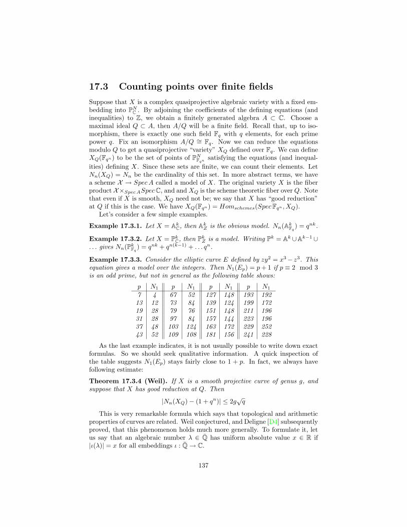
17.3 Counting points over finite fields
Suppose that X is a complex quasiprojective algebraic variety with a fixed em-bedding into PN
C . By adjoining the coefficients of the defining equations (andinequalities) to Z, we obtain a finitely generated algebra A ⊂ C. Choose amaximal ideal Q ⊂ A, then A/Q will be a finite field. Recall that, up to iso-morphism, there is exactly one such field Fq with q elements, for each primepower q. Fix an isomorphism A/Q ∼= Fq. Now we can reduce the equationsmodulo Q to get a quasiprojective “variety” XQ defined over Fq. We can defineXQ(Fqn) to be the set of points of PN
Fqnsatisfying the equations (and inequal-
ities) defining X. Since these sets are finite, we can count their elements. LetNn(XQ) = Nn be the cardinality of this set. In more abstract terms, we havea scheme X → SpecA called a model of X. The original variety X is the fiberproduct X×Spec ASpec C, and and XQ is the scheme theoretic fiber over Q. Notethat even if X is smooth, XQ need not be; we say that X has “good reduction”at Q if this is the case. We have XQ(Fqn) = Homschemes(Spec Fqn , XQ).
Let’s consider a few simple examples.
Example 17.3.1. Let X = AkC, then Ak
Z is the obvious model. Nn(AkFq
) = qnk.
Example 17.3.2. Let X = PkC, then Pk
Z is a model. Writing Pk = Ak ∪Ak−1 ∪. . . gives Nn(Pk
Fq) = qnk + qn(k−1) + . . . qn.
Example 17.3.3. Consider the elliptic curve E defined by zy2 = x3− z3. Thisequation gives a model over the integers. Then N1(Ep) = p + 1 if p ≡ 2 mod 3is an odd prime, but not in general as the following table shows:
p N1 p N1 p N1 p N1
7 4 67 52 127 148 193 19213 12 73 84 139 124 199 17219 28 79 76 151 148 211 19631 28 97 84 157 144 223 19637 48 103 124 163 172 229 25243 52 109 108 181 156 241 228
As the last example indicates, it is not usually possible to write down exactformulas. So we should seek qualitative information. A quick inspection ofthe table suggests N1(Ep) stays fairly close to 1 + p. In fact, we always havefollowing estimate:
Theorem 17.3.4 (Weil). If X is a smooth projective curve of genus g, andsuppose that X has good reduction at Q. Then
|Nn(XQ)− (1 + qn)| ≤ 2g√
q
This is very remarkable formula which says that topological and arithmeticproperties of curves are related. Weil conjectured, and Deligne [D4] subsequentlyproved, that this phenomenon holds much more generally. To formulate it, letus say that an algebraic number λ ∈ Q has uniform absolute value x ∈ R if|ι(λ)| = x for all embeddings ι : Q→ C.
137
Theorem 17.3.5 (Deligne). Let X be a smooth projective d dimensional va-riety and suppose that X has good reduction at Q. Then
Nn(XQ) =2d∑
i=0
(−1)ibi∑
j=1
λnji,
where λji are algebraic integers with uniform absolute values qi/2 and bi coin-cides with the ith Betti number of X.
See [H, appendix C] and especially [K] for a more involved discussion of thisand the other Weil conjectures. It is worth noting that the classical method ofLefschetz pencils play an important role in the proof. Deligne [D3], [D5] founda subsequent refinement which gives meaning to the mixed Betti numbers.
Theorem 17.3.6 (Deligne). Let X be a d dimensional variety Then
Nn(Xq) =2d∑
i=0
(−1)ibi∑
j=1
λnji
where λji are algebraic integers with uniform absolute values in 0, q1/2, q, . . . qi/2.bi = dim Hi
c(X, C) and
b(m)i (X) = #j | |λij | = qm/2
17.4 A transcendental analogue of Weil’s con-jecture
The discussion in the previous section may have a seemed a bit like black magic.It may be worthwhile to explain a little more about the philosophy behind it.Let X be a smooth projective variety defined over Fq, and X be the extensionof X to the algebraic closure Fq. Fix a prime ` different from the characteris-tic of Fq. If we choose an embedding X ⊂ PN , we have F : X → X be theFrobenius morphism which acts by raising the coordinates of the qth power (see[H] for a more precise description). Then Nn(X) is just the number of fixedpoints of Fn. Weil suggested that that these numbers could be computed byan appropriate generalization of Lefschetz’s trace formula. This was realized byGrothendieck’s `-adic cohomology theory [Mi], which assigns to X a collectionof finite dimensional Q`-vector spaces Hi
et(X, Ql) which behaves very much sin-gular cohomology of a complex variety. In particular, if X is obtained as inthe previous section by reducing modulo Q, dim Hi
et(X, Ql) coincides with theBetti number of the original complex variety. The Grothendieck-Lefschetz traceformula shows that
Nn(X) =∑
i
(−1)itrace[Fn∗ : Hiet(X, Ql)→ Hi
et(X, Ql)]
138
The λji of theorem 17.3.5 are precisely the eigenvalues of F acting on thesecohomology groups. Thus the real content of this theorem is the estimate onthese eigenvalues.
Around 1960, Serre [S3] had proved an analogue of theorem 17.3.5 for com-plex varieties. This is something that we can prove. To set up the analogy letus replace X above by a smooth complex projective variety Y , and F by andendomorphism f : Y → Y . As for q, if we consider, the effect of the Frobeniuson PN
Fq, the pullback of O(1) under this map is O(q). To complete the anal-
ogy, we require the existence of a very ample line bundle OY (1) on Y , so thatf∗OY (1) ∼= OY (1)⊗q. We can take c1(OY (1)) to be the Kahler class ω Then wehave f∗ω = qω.
Theorem 17.4.1 (Serre). If f : Y → Y is holomomorphic endomorphismof a compact Kahler manifold with Kahler class ω, such that f∗ω = qω forsome q ∈ R. Then the eigenvalues λ of f∗ : Hi(Y, Z) → Hi(Y, Z) are algebraicintegers with uniform absolute value qi/2
Proof. The theorem holds for H2n(Y ) since ωn generates it. By hypothesis,f∗ preserves the Lefschetz decomposition (theorem 13.1.1), thus we can replaceHi(Y ) by primitive cohomology P i(Y ). Recall from corollary 13.1.4,
Q(α, β) = Q(α, Cβ)
is positive definite Hermitean form P i(Y ), where
Q(α, β) = (−1)i(i−1)/2
∫α ∧ β ∧ ωn−i.
Consider the endomorphism F = q−i/2f∗ of P i(Y ). We have
Q(F (α), F (β)) = (−1)i(i−1)/2q−n
∫f∗(α ∧ β ∧ ωn−i) = Q(α, β)
Moreover, since f∗ is a morphism of Hodge structures, it preserves the Weiloperator C. Therefore F is unitary with respect to Q, so its eigenvalues havenorm 1. This gives the desired estimate on absolute values of the eigenvalues off∗. Since f∗ can be represented by an integer matrix, the set of it eigenvalues isa Galois invariant set of algebraic integers, so these have uniform absolute valueqi/2.
Grothendieck suggested that one should be able to carry out a similar prooffor the Weil conjectures. However making this work would require the fullstrength of his standard conjectures [GSt, Kl] which are, at present, very muchopen.
139
Bibliography
[AH] M. Atiyah, F. Hirzebruch, Analytic cycles on complex manifolds,Topology 1 (1962)
[AM] M. Atiyah, I. Macdonald, Commutative algebra, Adison-Wesley (1969)
[BPV] W. Barth, C. Peters, A. Van de Ven, Compact complex surfaces,Springer-Verlag (1984)
[Ch] I. Chavel, Eigenvalues in Riemannian geometry, Academic Press(1984)
[DK] V. Danilov, A. Khovanskii, Newton polyhedra and an algorithm forcomputing Hodge-Deligne numbers Math. USSR Izv. (1987)
[D1] P. Deligne, Theoreme de Lefschetz et criteres de degenerescence desuites spectrales Publ. IHES 35 (1968)
[D2] P. Deligne, Theorie de Hodge II, III, Publ. IHES, (1972, 1974)
[D3] P. Deligne, Poids dans la cohomologie des varietes algebriques., Proc.ICM (1974)
[D4] P. Deligne, Conjecture de Weil I, Publ. IHES, (1974)
[D5] P. Deligne, Conjecture de Weil II, Publ. IHES, (1980)
[DGMS] P. Deligne, P. Griffiths, J. Morgan, D. Sullivan, Real homotopy theoryof Kahler manifolds, Invent. Math. 29 (1975)
[SGA7] P. Deligne, N. Katz, SGA 7, II, Lect. Notes 340, Springer-Verlag (1973)
[E] D. Eisenbud, Commutative algebra Springer-Verlag (1994)
[EV] H Esnault, E. Viehweg, Lectures on vanishing theorems, Birkhauser(1993)
[M2] D. Eisenbud, D. Grayson, M. Stillman, B. Sturmfels, Computations inalgebraic geometry with Macaulay 2 Springer-Verlag (2001)
[F] W. Fulton, Toric varieties Princeton U. Press (1993)
140
[GM] S. Gelfand, Y. Manin, Methods of homological algebra, Springer-Verlag(1996)
[G] R. Godement, Toplogique algebriques et theorie de faiseaux, Hermann(1964)
[GPR] H. Grauert, T. Peternell, R. Remmert (Ed.) Several complex variablesVII, Springer-Verlag (1991)
[GH] P. Griffiths, J. Harris, Principles of algebraic geometry, John-Wiley(1978)
[GS] P. Griffiths, W. Schmid, Recent developements in Hodge theory, Proc.Bombay colloq. on Discrete subgroups of Lie groups, Tata Inst. (1975)
[EGA] A. Grothendieck, J. Dieudonne, Element de Geometrie Algebrique I,II, III, IV, Publ IHES (1961-1967)
[Gr] A. Grothendieck, Sur quelque point d’algebra homologique, TohokuMath. J. (1957)
[GSt] A. Grothendieck, Standard conjectures on algebraic cycles, Alg. Geom.,Bombay 1968, Tata Inst. (1969)
[Hs] J. Harris, Algebraic geometry. A first course. Springer-Verlag, (1992)
[HM] J. Harris, I. Morrison, Moduli of curves, Springer-Verlag (1998)
[H1] R. Hartshorne, Varieties of small codimension in projective space, Bull.AMS (1974)
[H] R. Hartshorne, Algebraic Geometry, Springer-Verlag (1977)
[Ha] H. Hironaka, Resolution of singularities of an algebraic variety over afield of characteristic 0, Ann. Math (1964)
[Hh] F. Hirzebruch, Topological methods in algebraic geometry, Springer-Verlag (1978)
[Ho] W. Hodge, The theory and applications of harmonic integrals. Cam-bridge (1941)
[Hr] L. Hormander, An introduction to several complex variables North Hol-land (1973)
[I] B. Iverson, Cohomology of Sheaves, Springer-Verlag (1986)
[K] N. Katz, An overview of Deligne’s proof of the Riemann hypothesis forvarieties over finite fields. Proc. Sympos. Pure Math., Vol. XXVIII,AMS (1976)
141
[Kl] S. Kleiman, Algebraic cycles and the Weil conjectures, Dix Esposes surla cohomologies les schemas, North Holland (1968)
[La] K. Lamotke, The topology of complex projective varieties after S. Lef-schetz. Topology (1981)
[L] S. Lefschetz, L’Analysis Situs et Geometrie Algebrique, Gauthier-Villars (1923)
[Lw] J. Lewis, A survey of the Hodge conjecture, CRM monogarph, AMS(1999)
[MR] A. Milgram, P. Rosenbloom, Harmonic forms and Heat conductionI,Proc. Nat. Acad. Sci. (1951)
[Mi] J. Milne, Etale cohomology, Princeton U. P (1980)
[Mo] B. Moishezon, On n-dimensional compact varieties with n algebraicallyindependent meromorphic functions, Izv. Akad Nauk SSSR (1966)
[MK] J. Morrow, K. Kodaira, Complex Manifolds, Holt, Rinehart, Winston(1971)
[M] D. Mumford, Red Book of Varieties and Schemes, Springer-Verlag(1988)
[MA] D. Mumford, Abelian varieties, Tata Institute (1969)
[S] J. P. Serre, Faiseaux algebriques coherents, Ann. Math. (1955)
[S2] J. P. Serre, Geometrie algebrique et geometrie analytique, Ann. Inst.Fourier (1956)
[S3] J. P. Serre, Analogue Kahlerian de Certaines Conjecture de Weil, Ann.Math (1960)
[S4] J. P. Serre, A course in arithmetic, Springer-Verlag (1973)
[Sh] I. Shafarevich, Basic Algebraic Geometry Springer-Verlag (1977)
[Sp] E. Spanier, Algebraic topology, McGraw-Hill (1966)
[Spv] M. Spivak, A comprehensive introduction to differential geometry I,Publish or Perish (1970)
[Wa] F. Warner, Foundations of the theory of differentiable manifolds andLie groups, Springer-Verlag (1983)
[Wl] C. Weibel, An introduction to homological algebra Cambridge (1994)
[W] R. Wells, Differential analysis on complex manifolds, Springer-Verlag(1979)
142