Complex Analysis

Xue-Mei Li

May 11, 2017

Contents

1 Prologue (Lecture 1) 3

2 Preliminaries 62.1 The complex plane . . . . . . . . . . . . . . . . . . . . . . . . . . . 62.2 Complex functions of one variables . . . . . . . . . . . . . . . . . . 62.3 Complex linear functions . . . . . . . . . . . . . . . . . . . . . . . . 82.4 Complex differentiation . . . . . . . . . . . . . . . . . . . . . . . . . 92.5 Holomorphic functions . . . . . . . . . . . . . . . . . . . . . . . . . 122.6 The ∂ and ∂ operator (Lecture 3) . . . . . . . . . . . . . . . . . . . . 122.7 Harmonic functions . . . . . . . . . . . . . . . . . . . . . . . . . . . 132.8 Rules of differentiation . . . . . . . . . . . . . . . . . . . . . . . . . 132.9 Problems . . . . . . . . . . . . . . . . . . . . . . . . . . . . . . . . 14

3 The Riemann sphere and Mobius transforms 163.1 Conformal mappings . . . . . . . . . . . . . . . . . . . . . . . . . . 163.2 Mobius transforms (Lecture 4-) . . . . . . . . . . . . . . . . . . . . . 17

3.2.1 The extended complex plane . . . . . . . . . . . . . . . . . . 183.2.2 Properties of Mobius transforms . . . . . . . . . . . . . . . . 18

3.3 The Riemann sphere and stereographic projection (Lecture 5) . . . . . 233.4 Problems . . . . . . . . . . . . . . . . . . . . . . . . . . . . . . . . 25

4 Power series 264.1 Power series is holomorphic in its disc of convergence (Lecture 6) . . 264.2 Analytic continuation . . . . . . . . . . . . . . . . . . . . . . . . . . 284.3 The exponential and trigonometric functions . . . . . . . . . . . . . . 304.4 The Logarithmic function and power function . . . . . . . . . . . . . 314.5 Problems . . . . . . . . . . . . . . . . . . . . . . . . . . . . . . . . 31

5 Complex integration 325.1 Integration along curves (Lecture 7) . . . . . . . . . . . . . . . . . . 325.2 Path independent property (Lecture 8) . . . . . . . . . . . . . . . . . 365.3 Existence of primitives . . . . . . . . . . . . . . . . . . . . . . . . . 375.4 Goursat’s Lemma and Cauchy’s Theorem for star regions . . . . . . . 395.5 Integration along homotopic curves . . . . . . . . . . . . . . . . . . 42

1

6 Cauchy’s integral formula (Lecture 11) 456.1 Cauchy’s integral formula . . . . . . . . . . . . . . . . . . . . . . . . 456.2 Taylor expansion, Cauchy’s derivative formulas (Lecture 12) . . . . . 476.3 Morera’s Theorem . . . . . . . . . . . . . . . . . . . . . . . . . . . 486.4 Cauchy’s inequality, and Liouville’s Theorem . . . . . . . . . . . . . 49

7 Analytic Functions 517.1 Schwartz Reflection Principle (Lecture 13) . . . . . . . . . . . . . . . 517.2 Locally uniform convergence (Lecture 14) . . . . . . . . . . . . . . . 537.3 zeros of analytic functions . . . . . . . . . . . . . . . . . . . . . . . 54

7.3.1 The Fundamental Theorem of Algebra . . . . . . . . . . . . . 547.3.2 Zeros of analytic functions (Lecture 15) . . . . . . . . . . . . 557.3.3 Maximum Modulus Principle (Lecture 16) . . . . . . . . . . 58

8 Laurent series and singularities 608.1 Cauchy’s formula and Laurent series (16-17) . . . . . . . . . . . . . 608.2 Classification of isolated singularities (Lecture 18) . . . . . . . . . . 65

8.2.1 Poles and Residues . . . . . . . . . . . . . . . . . . . . . . . 678.3 Meromorphic functions . . . . . . . . . . . . . . . . . . . . . . . . . 70

9 Winding numbers and Cauchy’s Theorems 719.1 Winding numbers (Lecture 21) . . . . . . . . . . . . . . . . . . . . . 719.2 Winding numbers and Cauchy’s Theorem . . . . . . . . . . . . . . . 73

9.2.1 Supplementary . . . . . . . . . . . . . . . . . . . . . . . . . 769.3 The Residue Theorem (Lecture 23) . . . . . . . . . . . . . . . . . . . 779.4 Compute real integrals . . . . . . . . . . . . . . . . . . . . . . . . . 77

10 Argument Principle and Rouche’s Thoerem 7910.1 The Argument Principle (Lecture 24) . . . . . . . . . . . . . . . . . . 7910.2 Rouche’s Theorem (Lecture 24) . . . . . . . . . . . . . . . . . . . . 80

10.2.1 Supplementary . . . . . . . . . . . . . . . . . . . . . . . . . 8110.3 The open mapping theorem (lecture 24) . . . . . . . . . . . . . . . . 81

10.3.1 Supplementary . . . . . . . . . . . . . . . . . . . . . . . . . 8210.4 Hurwitz’s theorem (lecture 24) . . . . . . . . . . . . . . . . . . . . . 83

11 The Riemann Mapping Theorem 8511.1 Family of holomorphic functions (Lecture 25) . . . . . . . . . . . . . 8511.2 Bi-holomorphic maps on the disc . . . . . . . . . . . . . . . . . . . . 8811.3 The Riemann mapping theorem (Lecture 28-29) . . . . . . . . . . . . 9011.4 Supplementary . . . . . . . . . . . . . . . . . . . . . . . . . . . . . 92

12 Special functions 9312.1 Constructing holomorphic functions by integration (Lecture 30) . . . 9312.2 The Gamma function . . . . . . . . . . . . . . . . . . . . . . . . . . 9312.3 The zeta function (Lecture 30) . . . . . . . . . . . . . . . . . . . . . 94

2

Chapter 1

Prologue (Lecture 1)

This is the lecture notes for the third year undergraduate module: MA3B8.Complex numbers are useful where the cosine and sine functions appear. This is

used in electric engineering for analysis of alternating circuit where the voltage func-tion is given by V (t) = Re(V0e

i(ωt+φ)) = V0 cos(ωt + φ). For example for a simplecircuit in an English home, V0 = 220

√2 and ω = 50(2π), the frequency is 50 Hz with

average voltage 220. Addition using complex numbers is convenient here. In radio en-gineering, V (t) = A cos(2πFt+φ0) is used for amplitude and frequency modulations.The Schrodinger equation,

i~∂ψ

∂t= − ~2

2m

∂2ψ

∂2x+ V (x)ψ(t, x),

a fundamental equation of physics, that describes how a wave function of a physicalsystem evolves. Complex valued functions are built into the definition for Fouriertransforms, an important tool in analysis and engineering. For f : R→ R,

f(k) =1√2π

∫ ∞−∞

e−ikxf(x)dx, k ∈ R.

Fourier transform extends the concept of Fourier series for period functions, is an im-portant tool in analysis and in image and sound processing, and is widely used in elec-trical engineering.

Complex Analysis is concerned with the study of complex number valued functionswith complex number as domain. Let f : C→ C be such a function. What can we sayabout it? Where do we use such an analysis?

Complex Differentiation is a very important concept, this is allured to by the factthat a number of terminologies are associated with ‘complex differentiable’. A func-tion, complex differentiable on its domain, has two other names: a holomorphic mapand an analytic function, reflecting the original approach. The first meant the functionis complex differentiable at every point, and the latter refers to functions with a powerseries expansion at every point. The beauty is that the two concepts are equivalent. Acomplex valued function defined on the whole complex domain is an entire function.Quotients of entire functions are Meromorphic functions on the whole plane.

A map is conformal at a point if it preserves the angle between two tangent vec-tors at that point. A complex differentiable function is conformal at any point whereits derivative does not vanish. Bi-holomorphic functions, a bi-jective holomorphic

3

function between two regions, are conformal in the sense they preserve angles. Of-ten by conformal maps people mean bi-holomorphic maps. Conformal maps are thebuilding blocks in Conformal Field Theory. It is conjectured that 2D statistical mod-els at criticality are conformal invariant. An exciting development is SLE, evolvedfrom the Loewner differential equation describing evolutions of conformal maps. TheSchramann-Loewner Evolution (also known as Stochastic Loewner Evolution, abbre-viated as SLE ) has been identified to describe the limits of a number of lattice modelsin statistical mechanics. Two mathematicians, W. Werner and S. Smirnov, have beenawarded the Fields medals for their works on and related to SLE.

A well known function in number theory is the Riemann zeta-function,

ζ(s) =

∞∑n=1

1

ns.

The interests in the Riemann-zeta function began with Euler who discovered that theRiemann zeta function can be related to the study of prime numbers.

ζ(s) = Π1

1− p−s.

The product on the right hand side is over all prime numbers:

Π1

1− p−s=

1

1− 2−s· 1

1− 3−s· 1

1− 5−s· 1

1− 7−s· 1

1− 11−s. . .

1

1− p−s. . . .

The Riemann-zeta function is clearly well defined for |s| > 1 and extends to all com-plex numbers except s = 1, a procedure known as the analytic /meromorphic contin-uation of a real analytic function. Riemann was interested in the following question:how many prime number are below a given number x? Denote this number π(x). Rie-mann found an explicit formula for π(x) in his 1859 paper in terms of a sum over thezeros of ζ. The Riemann hypothesis states that all non-trivial zeros of the Riemannzeta function lie on the critical line s = 1

2 . The Clay institute in Canada has offered aprize of 1 million dollars for solving this problem.

In symplectic geometry, symplectic manifolds are often studied together with acomplex structure. The space C is a role model for symplectic manifold. A 2-dimensionalsymplectic manifold is a space that looks locally like a piece of R2 and has a symplecticform, which we do not define here. We may impose in addition a complex structure Jxat each point of x ∈M . The complex structure Jx is essentially a matrix s.t. −J2

x is theidentity and defines a complex structure and leads to the concept of Khaler manifolds.

We also note the Riemann-Hilbert problem. Given an oriented simple contour γ,find a function f that is analytic on C \ {γ} such that the limits of f from inside andfrom the outside satisfy the boundary condition on γ: f− = f+G and as f appraochesthe identity as z →∞.

Finally we should mention that complex analysis is an important tool in combinato-rial enumeration problems: analysis of analytic or meromorphic generating functionsprovides means for estimating the coefficients of its series expansions and estimatesfor the size of discrete structures.

TopicsHolomorphic Functions, meromorphic functions, poles, zeros, winding numbers (rota-tion number/index) of a closed curve, closed curves homologous to zero, closed curves

4

homotopic to zero, classification of isolated singularities, analytical continuation, Con-formal mappings, Riemann spheres, special functions and maps. Main Theorems:Goursat’s theorem, Cauchy’s Theorem, Cauchy’s derivative formulas, Cauchy’s inte-gral formula for curves homologous to zero, the Weirerstrass Theorem, The ArgumentPrinciple, Rouche’s Theorem, the open mapping theorem, Maximum Modulus Prin-ciple, Schwartz’s Lemma, Mantel’s Theorem, Hurwitz’s Theorem, and the RiemannMapping Theorem.

References• L. V. Ahlfors, Complex Analysis, Third Edition, Mc Graw-Hill, Inc. (1979)

• J. B. Conway. Functions of one complex variables.

• T. Gamelin. Complex Analysis, Springer. (2001)

• E. Hairer, G. Wanner, Analyse Complexe et Series de Fourier.http://www.unige.ch/hairer/poly_complexe/complexe.pdf

• G. J. O. Jameson. A First course on complex functions. Chapman and Hall,(1970).

• Theory of functions of onea complex variable. E. T. Copson. Oxford UniversityPress. (1935).

• E. M. Stein and R. Shakarchi. Complex Analysis. Princeton University Press.(2003)

Acknowledgement. I would like to thank E. Hairer and G. Wanner for the figures inthis note.

5

Chapter 2

Preliminaries

2.1 The complex planeThe complex plane C = {x+ iy : x, y ∈ R} is a field with addition and multiplication,on which is also defined the complex conjugation x+ iy = x− iy and modulus (alsocalled absolute value) |z| =

√zz =

√x2 + y2. It is a vector space over R and over C

with the norm |z1 − z2|.We will frequently treat C as a metric space, with distance d(z1, z2) = |z1 − z2|,

and so we understand that a sequence of complex numbers zn converges to a complexnumber z is meant by that the distance |zn − z| converges to zero. The space C withthe above mentioned distance is a complete metric space and so a sequence convergesif and only if it is a Cauchy sequence. Since

|zn − z|2 = |Re(zn)− Re(z)|2 + |Im(zn)− Im(z)|2,

zn converges to z if and only if the real parts of (zn) converge to the real part of z andthe imaginary parts of (zn) converge to the imaginary part of z.

In polar Coordinates z ∈ C can be written as z = reiθ where r = |z| and θ is a realnumber, called the argument. We note specially Euler’s formula:

eiθ = cos(θ) + i sin(θ),

so arg z is a multi valued function. It is standard to take the principal value −π <Argz ≤ π, a rather arbitrary choice.

Since e2πik = 1 for k an integer, the nth root function is multi-valued. If

ωk = e2πkn i, k = 0, 1, . . . , n− 1,

the nth roots of the unity, then

(reiθ)1n = r

1n ei

θnωk.

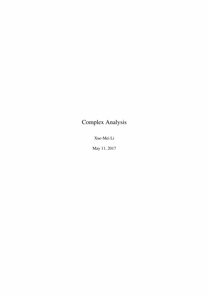
2.2 Complex functions of one variablesTo discuss complex differentiation of a function, we request that it is defined on a subsetof the complex plane C which is open. By a set we would usually mean a subset of the

6

−1 1

−1

1

−1 1

−1

1

zc

w = c z

c

Figure 2.1: Graph by E. Hairer and G. Wanner

complex plane C. A set U is open if about every point in U there is a disc containedentirely in U . We further assume that the set is connected, otherwise we could treat itas a separate function on each connected subset.

A subset of C is connected if any two points from the subset can be connected by acontinuous curve which lies entirely within the subset.

An open set is connected if and only if it is not disconnected in the sense that it isnot the union of two disjoint open sets.

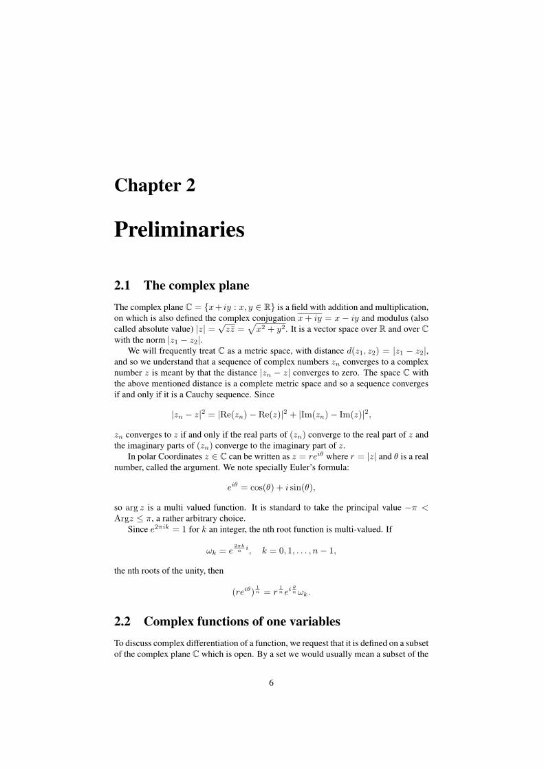
Example 2.2.1 Define f(z) = z2 whose maximal domain of definition is C. Writef = u+ iv. Then

u(x, y) = x2 − y2, v(x, y) = 2xy.

It is easy to see that f takes the horizontal lines y = b where b 6= 0 to parabolas onthe w plane facing right. Solve the equations: x2 − b2 = u and v = 2xb to see

u =1

4b2v2 − b2.

Also, f takes the vertical lines x = a where a 6= 0 to parabolas on the w plane facingleft.

u = 4a2 − 1

4a2v2.

These two sets of parabolas intersect at right angles, see Figure 2.2.If b = 0, the line y = 0 is mapped to the right half of the real axis; the line x = 0 is

mapped to the left half of the real axis. We observe that at 0, these two curves, imagesof the real and complex line from the domain space, fail to intersects with each otherat a right angle. (0 is the only point at which f ′ = 0, explaining the orthogonality andfailing of the orthogonality where the image curves meet, to which we return later.)

7

−1 0

−1

1

−1 1

−1

1

z =√w

w = z2

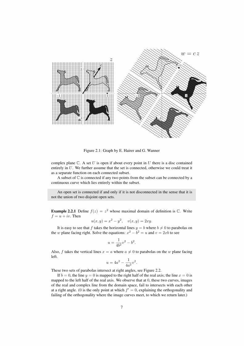
Figure 2.2: Graph by E. Hairer and G. Wanner

Example 2.2.2 The function f(z) = z2 is not injective. It takes the line y = b andy = −b to the same image. Define f on C \ (−∞, 0] by f(w) =

√w, the principal

brach of the square root function. So f(reiθ) =√reiθ/2, −π < θ < π. It has another

formula:f(w) =

√|w|ei(Argw/2), w ∈ C \ (−∞, 0].

It maps the slitw plane into the right half of the z-plane. The other branch of the squareroot is −

√w = ω2f(w). It is possible to glue the two slit domains together to form

a complex manifold, known as a Riemann surface, so in one sheet (chart) the functiontakes the value of one brach and in the other we use the other brach in a way f changescontinuously as w changes.

2.3 Complex linear functionsWe identify R2 with C. A function T : R2 → R2 is real linear if for all z1, z2, z ∈ R2,

T (z1 + z2) = T (z1) + T (z2),

T (rz) = rT (z), ∀r ∈ R

A map T : C→ C is complex linear if for all z1, z2, z ∈ C,

T (z1 + z2) = T (z1) + T (z2),

T (kz) = kT (z), ∀k ∈ C

Proposition 2.3.1 A real linear function T : R2 → R2 is complex linear iff

T (i) = iT (1).

8

We now look at the matrix representations. Every real linear map is of the form(xy

)→(a bc d

)(xy

).

As a set we identify a complex number s + it with the pair of real numbers (s, t),so C is identified with R2. Since, for z = x+ iy and k = s+ it,

k(x+ iy) = (sx− ty) + i(tx+ sy),

If k = s+ it, the complex linear map T (z) = kz is given by

T

(xy

)=

(s −tt s

)(xy

).

Multiplication by i is the same as multiply by J on the left, where

J =

(0 −11 0

).

For every real linear map T there exists a unique pair of complex numbers λ and µsuch that

T (z) = λz + µz,

which is complex linear if and only if µ = 0. Furthermore,

λ =1

2

((a+ ic) +

1

i(b+ id)

), µ =

1

2

((a+ ic)− 1

i(b+ id)

)

2.4 Complex differentiation

Definition 2.4.1 By a region we mean a connected open subset of C. By a properregion we mean an open connected subset of C that is not the whole complex plane.

From now on, by a function we mean a function f : U → C where U is a region.Let f = u + iv, defined in a region U . When C is identified as R2 we may treat

u and v as real valued functions on R2. In this way f is an R2 valued function of tworeal variables x and y. Then f is (real) differentiable at (x0, y0) if there exists a linearmap (df)(x0,y0) : R2 → R2 and a function φ such that

f(x, y) = f(x0, y0) + (df)(x0,y0)

(x− x0

y − y0

)+ φ(x, y)

∣∣∣∣(x− x0

y − y0

)∣∣∣∣ (2.4.1)

where φ satisfies φ(x0, y0) = 0 and lim(x,y)→(x0,y0) φ(x, y) = 0. Note that∣∣∣∣(x− x0

y − y0

)∣∣∣∣ = |z − z0|.

9

The linear function is represented by the Jacobian matrix.

Jf (x0, y0) =

(∂∂xu

∂∂yu

∂∂xv

∂∂yv

)(x0, y0).

The partial derivatives of f are denoted by

∂xf =

(∂∂xu∂∂xv

), ∂yf =

(∂∂yu∂∂y v

). (2.4.2)

Treated as a complex function,

∂xf =∂

∂xu+ i

∂

∂xv, ∂yf =

∂

∂yu+ i

∂

∂yv.

Definition 2.4.2 A function f : U → C is complex differentiable at z0 if there exists acomplex number f ′(z0) and a function ψ with ψ(z0) = 0 and limz→z0 ψ(z) = 0, suchthat

f(z) = f(z0) + f ′(z0)(z − z0) + ψ(z) |z − z0| . (2.4.3)

The number f ′(z0) is the derivative of f at z0.

Equivalently, f is complex differentiable at z0 with derivative f ′(z0) if and only if

f ′(z0) = limw→0

f(w + z0)− f(z0)

w.

Example 2.4.1 f(z) = z is differentiable. So are any polynomials in z.

This follows fromf(z0 + z)− f(z0)

z= 1

and chain rules.

Example 2.4.2 The function f(z) = z is not complex differentiable.

Proof Note

f(z0 + z)− f(z0)

z=z

z=

{1, if Im(z) = 0−1, if Re(z) = 0,

which means limz→0f(z0+z)−f(z0)

z does not exist. �

Definition 2.4.3 A function is differentiable in U if it is differentiable everyewherein U .

Notation. A function f : Rn → Rm is Cr if it is r times differentiable and itspartial derivatives of order less or equal to r are continuous.

10

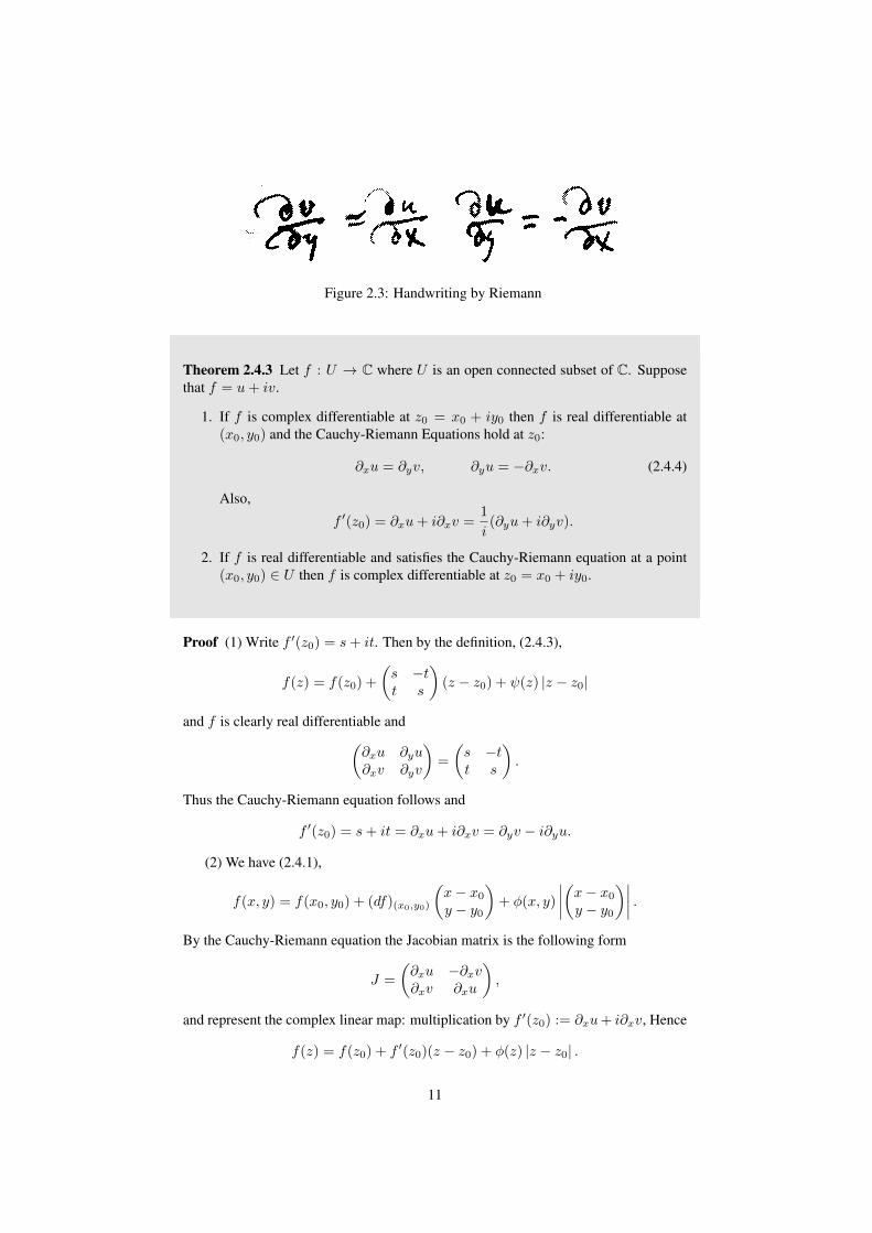
Figure 2.3: Handwriting by Riemann

Theorem 2.4.3 Let f : U → C where U is an open connected subset of C. Supposethat f = u+ iv.

1. If f is complex differentiable at z0 = x0 + iy0 then f is real differentiable at(x0, y0) and the Cauchy-Riemann Equations hold at z0:

∂xu = ∂yv, ∂yu = −∂xv. (2.4.4)

Also,

f ′(z0) = ∂xu+ i∂xv =1

i(∂yu+ i∂yv).

2. If f is real differentiable and satisfies the Cauchy-Riemann equation at a point(x0, y0) ∈ U then f is complex differentiable at z0 = x0 + iy0.

Proof (1) Write f ′(z0) = s+ it. Then by the definition, (2.4.3),

f(z) = f(z0) +

(s −tt s

)(z − z0) + ψ(z) |z − z0|

and f is clearly real differentiable and(∂xu ∂yu∂xv ∂yv

)=

(s −tt s

).

Thus the Cauchy-Riemann equation follows and

f ′(z0) = s+ it = ∂xu+ i∂xv = ∂yv − i∂yu.

(2) We have (2.4.1),

f(x, y) = f(x0, y0) + (df)(x0,y0)

(x− x0

y − y0

)+ φ(x, y)

∣∣∣∣(x− x0

y − y0

)∣∣∣∣ .By the Cauchy-Riemann equation the Jacobian matrix is the following form

J =

(∂xu −∂xv∂xv ∂xu

),

and represent the complex linear map: multiplication by f ′(z0) := ∂xu+ i∂xv, Hence

f(z) = f(z0) + f ′(z0)(z − z0) + φ(z) |z − z0| .

11

This implies f is complex differentiable at z0. �

The Cauchy Riemann equation can also be written as ∂xf = 1i ∂yf . Observe also

that if u, v, as real valued functions on R2 with continuous first order partial derivatives,then each u and v are real differentiable, and so is f .

2.5 Holomorphic functions

Definition 2.5.1 A function f : U → C is said to be holomorphic on U if it is differ-entiable at every point of U . A function f : C→ C is said to be entire if it is complexdifferentiable at every point of C.

The following proposition has a stronger version, see Corollary 5.2.5.

Proposition 2.5.1 Let U be a region. A holomorphic function in U with vanishingderivative must be a constant.

Proof To see this, we first note that f has vanishing Jacobian matrix, and so it deriva-tives along the coordinate directions vanishes. So f is constant along any line segmentparallel with x and y axis. But any two points in a connected open subset of the planecan be connected by piecewise line segments parallel to either x and y axis, lying en-tirely inside the open set. So the values of f at these two points must be the same.

�

Example 2.5.2 Let U be a region in C. If f : U → C is real valued, then f is notholomorphic in U unless f is a constant.

Proof Let f = u + iv where v vanishes identically. If f is holomorphic, by theCauchy-Riemann equation, ∂xu = ∂yu = 0 and f ′(z) = ∂yv + i∂xv = 0, and f mustbe a constant. �

2.6 The ∂ and ∂ operator (Lecture 3)Given a function f , we have

f(x, y) = f

(z + z

2,z − z

2i

).

This inspires the notation :

∂z =1

2(∂

∂x+

1

i

∂

∂y), ∂z =

1

2(∂

∂x− 1

i

∂

∂y). (2.6.1)

It is common to denote ∂z by ∂ and ∂z by ∂. We can reformulate the earlier theoremusing these notations.

12

Suppose that f is complex differentiable at z then f is real differentiable at z and,

∂f(z) = 0, f ′(z) = ∂f(z).

Just note that ∂f = 12 ( ∂∂xu+ i ∂∂xv)− 1

2i (∂∂yu+ i ∂∂yv) and

f ′ = ∂xf =1

i

∂

∂yf =

1

2(∂

∂xf +

1

i

∂

∂yf) = ∂f.

2.7 Harmonic functions

Definition 2.7.1 A real valued function u : R2 → R is a harmonic function if ∆u = 0where ∆ = ∂xx + ∂yy is the Laplacian.

Proposition 2.7.1 If u, v areC2 functions and satisfies the Cauchy-Riemann equations

∂xu = ∂yv, ∂yu = −∂xv,

then u, v are harmonic functions. Consequently u, v are C∞.

Proof We differentiate the Cauchy-Riemann equation to see

∂xxu = ∂xyv, ∂yyu = −∂yxv.

Consequently ∂xxu + ∂yyu = 0. Similarly, ∂xxv + ∂yyv = 0. From standard theoryin PDE, a solution of the elliptic equation ∆u = 0 is C∞. �

Later we see that if f is differentiable in a region, it has derivatives of all orders.So the conditions u, v ∈ C2 can be reduced to C1.

2.8 Rules of differentiationTheorem 2.8.1 If f, g are differentiable at z0, the derivatives indicated below exist atz0 and the relations stated below hold when evaluated at z0.

1. (kf)′ = kf ′, for any k ∈ C

2. (f + g)′ = f ′ + g′

3. (fg)′ = fg′ + f ′g

4. (f/g)′ = gf ′−fg′g2 provided g(z0) 6= 0.

Theorem 2.8.2 Suppose that g is differentiable at z0 and f is differentiable at g(z0)then the composition f ◦ g is differentiable at z0 and

(f ◦ g)′(z0) = f ′(g(z0)) g′(z0).

13

Observe that if the Jacobian matrix of a complex differentiable function f repre-sents complex multiplication, i.e. it is of the form

J =

(∂xu ∂yu−∂yu ∂xu

),

then so is its inverse:

J−1 =1

det J

(∂xu −∂yu∂yu ∂xu

).

Since f ′(z0) = ∂xu(z0)− i∂yu(z0),

1

f ′(z0)=

∂xu(z0) + i∂yu(z0)

(∂xu)2(z0) + (∂yu(z0))2=

1

det J(z0)(∂xu(z0) + i∂yu(z0)),

then J−1(z0) represents 1f ′(z0) .

Theorem 2.8.3 Let f : U → C be holomorphic. Suppose f ′(z0) 6= 0 for somez0 ∈ U .

Then there exists a disc U around z0 such that f : D → f(D) is a bijection, f(D)is open and f−1 is complex differentiable on f(D) and

(f−1)′(f(z)) =1

f ′(z), z ∈ D.

Proof We learn later that the holomorphic assumption implies that the real and imag-inary parts of f are C1. Then f ′ does not vanish on a disc D of U , from which f is abijection to its image and f−1 is continuous, and hence f(D) is open. To see that f−1

is differentiable at a point w1 ∈ f(D), let w1 = f(z1) and w = f(z). Since f and f−1

are continuous, w → w1 is equivalent to z → z1. Since f ′(z1) 6= 0,

f−1(w)− f−1(w1)

w − w1=

1f(z)−f(z1)

z−z1

.

Take w → w1 we see that the limit on the left hand side exists and

f−1(w1) =1

f ′(z1)=

1

f ′(f−1(w)).

�

Remark 2.8.4 Later we see that if f is complex differentiable, it is infinitely differen-tiable. If f is one to one then f ′ does not vanish. See section 10.3.

2.9 Problems

Exercise 2.9.1 Let f = u + iv. Set J =

(0 −11 0

). Prove that Cauchy-Riemann

equations are equivalent to dfJ = Jdf where df is the Jacobian matrix of f .

14

Exercise 2.9.2 Suppose that f : U → C is complex differentiable where U is a region.Define U∗ := {z : z ∈ U}. Prove that g : U∗ → C given by the formula

g(z) = f(z)

is complex differentiable. Write the derivative of g in terms of f .

Exercise 2.9.3 Let log z := log |z| + i arg z. Use the Cauchy-Riemann equation toprove that the logarithm function log : C \ (−∞, 0]→ C is holomorphic.

Exercise 2.9.4 Let f : {a+ ib : a > 0} → C\ (−∞, 0] be the function z 7→ z2. Provethat f−1 is holomorphic.

Exercise 2.9.5 Determine at which points the following functions are differentiable:

zRe(z),z

|z|2, zz.

Exercise 2.9.6 Find all holomorphic functions f whose real part is u(x, y) = 2xy +2x.

Exercise 2.9.7 If F ′(z) = f(z) in a region D we say F is a primitive of f . Prove thatf(z) = |z|2 does not have a primitive. (Hint: Use Cauchy-Riemann equation.)

Exercise 2.9.8 Let r be a non-zero real number, c a real number and k ∈ C, satisfyingthe relation |k|2 > cr. Prove that the equation

r|z|2 − kz − kz + c = 0.

represents a circle. Determine its centre and radius.

Exercise 2.9.9 Let c ∈ R and k ∈ C. Prove that kz + kz + c = 0 represents a straightline.

Exercise 2.9.10 let f : C \ {0} → C \ {0} be the inversion f(z) = 1z . Prove that f

takes a circle to a circle or a line. Hint. Use Exercise 2.9.11.

Exercise 2.9.11 Let r be a positive number and a, b ∈ C. Prove that the equation|z − a| = r|z − b| determines a circle or a line.

15

Chapter 3

The Riemann sphere andMobius transforms

3.1 Conformal mappingsDefinition 3.1.1 A parameterized curve in the complex plane is a function z : [a, b]→C where [a, b] is closed interval of R.

If z(t) = x(t) + iy(t) its derivative is z′(t) = x′(t) + iy′(t).

Definition 3.1.2 The parameterized curve : [a, b] → C is smooth if z′(t) exists and iscontinuous on [a, b]. We assume furthermore z′(t) 6= 0.

The derivatives at the ends are understood to be one sided derivatives. From now on bya curve we mean a smooth curve.

If z′(t) does not vanish the curve has a tangent at this point, whose direction isdetermined by arg(z′(t)).

Definition 3.1.3 Let z1 : [a1, b1] → C and z2 : [a2, b2] → C be two smooth curvesintersecting at z0. The angle of the two curves is the angle of their derivatives at thispoint.

They are given by the difference of the arguments of their derivatives. If z1(t1) =z2(t2) = z0, their angle at the point z0 is: arg(z′2(t2))− arg(z′1(t1)).

Definition 3.1.4 A map f : U → C is conformal at z0 if it preserves angles, i.e. if z1

and z2 are two curves meeting at z0, the angle from f ◦ z1 to f ◦ z2 at f(z0) are thesame as the angle from z1 to z2 at z0.

A holomorphic function that preserves angles is called a conformal map.

Example 3.1.1 1. Given z0 ∈ C, the function f : C → C given by the formulaf(z) = z + z0 is said to be a translation, a conformal map.

2. Let c 6= 0 be a complex number, the function f(z) = cz is of the form below.For z = x+ iy, c = |c| eiθ,(

xy

)7→ |c|

(cos(θ) − sin(θ)sin(θ) cos(θ)

)(xy

).

16

This is the composition of a rotation by an angle θ and a scaling by |c|. This mappreserves the angle between two vectors, a conformal map.

3. The f(z) = z is not a conformal map, it reverses orientation.

Theorem 3.1.2 If f : U → C is holomorphic at z0 and f ′(z0) 6= 0, then f is conformalat z0.

Proof Let z1 : [a1, b1] → C and z2 : [a2, b2] → C be two smooth curves intersectingat z0: for t1 ∈ [a1, b1] and t2 ∈ [a2, b2], z1(t1) = z2(t2) = z0. Let γ1(t) = f ◦ z1(t)and γ2(t) = f ◦ z2(t). Since f ′(z0) does not vanish, γ1 and γ2 have well definedtangents which are:

γ′(t1) =d

dt|t=t1f ◦ z1 = f ′(z1(t1))z′1(t1) = f ′(z0)z′1(t1)

γ′(t2) =d

dt|t=t2f ◦ z2 = f ′(z2(t2))z′2(t2) = f ′(z0)z′2(t2).

Multiply z′1(t1) and z′1(t1) by the non-zero complex number f ′(z0) preserves anglesbetween the two vectors, as well as their orientation, c.f. Example ??, so the anglefrom γ1 to γ2 at f(z0) is the same as the angle from z1 to z2 at z0. �

Note also,arg(γ′(t1)) = arg(f ′(z0)) + arg(z′1(t1)).

Example 3.1.3 The map f(z) = 1z , the inversion map, is defined on C\{0}. It is easy

to see that f takes circles centred at the origin to circles centres at the origin. It take thelocus of the solutions of |z − z0| = r to that of a circle in the w-plane, see Proposition3.2.6.

Example 3.1.4 f(z) = z2 is conformal at any point z 6= 0. At z = 0 it is notconformal.

3.2 Mobius transforms (Lecture 4-)A polynomial P (z) = a0 + a1z + . . . anz

n, where ai ∈ C, is an entire function. Theroots zn are the zeros of P . If there are exactly r roots coincide, this root is said tohave order r. In light of Theorem 3.1.2 it is interesting to know where lie the zeros ofP ′(z).

By the fundamental theorem of Algebra, which we prove later (Theorem 7.3.2),P (z) = 0 has a complete factorisation:

P (z) = an(z − z1) . . . (z − zn).

Suppose that P and Q are two polynomials without common factors and define therational function

f(z) =P (z)

Q(z).

Then f is defined and is complex differentiable everywhere except at the zeros’ of Q.The zeros of Q are the poles of f . We now look at rational functions with one pole andone zero.

17

Definition 3.2.1 The following collection of maps are Mobius transforms{az + b

cz + d: ad− bc 6= 0, a, b, c, d,∈ C

}.

Note that multiply a, b, c, d, by a non-zero number λ does not change the function

f(z) =az + b

cz + d=azλ+ bλ

cλz + dλ.

If ad−bc = 0, az+bcz+d is a constant function, and are hence excluded. We may eliminateone parameter and assume that ad− bc = 1.

If f(z) = az+bcz+d is a Mobius transform, its maximal domain in C is: C \ {−dc}.

Sincef ′(z) =

ad− bc(cz + d)2

6= 0,

f is a conformal map.

3.2.1 The extended complex planeTo make the statements neat we add a point at infinity to C and define the extendedcomplex plane to be

C = C ∪ {∞}

with the convention:

1

0=∞, 1

∞= 0, a+∞ =∞, a−∞ =∞,

and for a 6= 0, a · ∞ =∞ · a =∞.

3.2.2 Properties of Mobius transformsLet f(z) = az+b

cz+d . We extend the Mobius transform f from C to C by defining:

f(−dc

) =∞, f(∞) =a

cif c 6= 0.

If c = 0, f(z) = 1f (az + b) is defined on the whole plane, then we define f(∞) =∞.

The function f has an inverse

f−1(w) =dw − b−cw + a

.

We define

M =

{z 7→ az + b

cz + d: ad− bc = 1, a, b, c, d,∈ C

}.

We stress that multiplying a, b, c, d by a non-zero number λ does not change the map.The following theorem states that any Mobius transform is a composition of transla-tions, scalings, and inversions.

Theorem 3.2.1 The setM of Mobius transforms is a group under composition. EachMobius transform is a composition of the following maps:

18

(1) translation: z 7→ z + a for some complex number a;

(2) composition of scaling (by a non-zero number ) and rotation:

z 7→ kz, some k ∈ C, k 6= 0.

(3) Inversion: z 7→ 1z .

In particular Mobius transforms are bijections of the extended complex plane.

Proof For the group we check the following:

• f(z) = z is the identity. (a = 1, b = c = 0, d = 1)

• If f(z) = az+bcz+d ∈M, then

f−1(w) =dw − b−cw + a

∈M.

• If f(z) = az+bcz+d ∈ M and g(z) = a′z+b′

c′z+d′ ∈ M. Then f ◦ g = Az+BCz+D ∈ M

where the complex numbers A,B,C,D are given by(A BC D

)=

(a bc d

)(a′ b′

c′ d′

).

For the second part of the statement, if c = 0, az+bd = adz + b

d . If c 6= 0,

f(z) =az + b

cz + d=a

c− 1

c21

z + dc

.

We note that translations, multiplication by a non-zero number are bijections of C, andthe extended complex plan if we send∞ to∞. The inversion map z 7→ 1

z and 0→∞,∞→ 0 is also a bijection. �

We make the following remark whose context is beyond the scope of the course.If we denote by PSL(2,C) the projective special linear map, it is the quotient of thespecial linear map with its subgroup Z of diagonal matrices, then the mobius transformaz+bcz+d to the matrix

(a bc d

)∈ PSL(2,C) is a group isomorphism, and Mobius trans-

forms are projective transformations of complex projective lines. The complex projec-tive line is a non-zero complex number with the equivalent relation (z, w) ∼ (λz, λw)where λ ∈ C \ {0}. Thus every Mobius transform is a bijection of the extended com-plex plane.

Example 3.2.2 The map f(z) = z+1z−1 is called the Cayley transform. It takes C \ {1}

to itself, f : C \ {1} → C \ {1} is a bijection and f−1 = f . Let us consider f as a mapon C = C ∪ {∞} by setting f(1) =∞, f(∞) = 1. Note

f(x+ iy) =x2 + y2 − 1

(x− 1)2 + y2+

−2y

(x− 1)2 + y2i.

Let γ = {x2 + y2 = 1} with γ+ and γ− denote respectively the upper and lower halfof the circle. Then,

19

• f sends {−1, 0, 1} to {0,−1,∞} respectively.

• f sends the upper circle to the lower half of the imaginary axis.

• f sends x-axis to x-axis. It send the x-axis within the unit disc to the negativex-axis.

• f sends the upper half of the unit disc to the third quadrant.

• f sends the lower circle to the upper half of the imaginary axis.

• f sends the lower half of the unit disc to the second quadrant.

• f sends the exterior of the unit circle to the right half of the plane.

If z2, z3, z4 are distinctive points in the extended plane C we associate to it the Mobiustransform

Fz2z3z4(z) =z − z3

z − z4/z2 − z3

z2 − z4=

(z − z3)(z2 − z4)

(z2 − z3)(z − z4), if z2, z3, z4 ∈ C.

If one of these points is the point at infinity the map is interpreted as following:

Fz2z3z4(z) =

z − z3

z − z4, if z2 =∞

z2 − z4

z − z4, if z3 =∞

z − z3

z2 − z3, if z4 =∞.

Note that if z2, z3, z4 ∈ C,

Fz2z3z4(z2) = 1, Fz2z3z4(z3) = 0, Fz2z3z4(z4) =∞.

That is, Fz2z3z4 take {z2, z3, z4} to {1, 0,∞}. Also,

If z2 =∞, Fz2z3z4(∞) = 1, Fz2z3z4(z3) = 0, Fz2z3z4(z4) =∞,If z3 =∞, Fz2z3z4(z2) = 1, Fz2z3z4(∞) = 0, Fz2z3z4(z4) =∞,If z4 =∞, Fz2z3z4(z2) = 1, Fz2z3z4(z3) = 0, Fz2z3z4(∞) =∞.

Lemma 3.2.3 A Mobius transform can have at most two fixed points unless f(z) isthe identity map.

Proof We solve for az+bcz+d = z, equivalently cz2 + (d− a)z − b = 0. This has at mosttwo solutions(use polynomial long division/ the Euclidean algorithm). �

Proposition 3.2.4 For any two sets of distinctive complex numbers {z2, z3, z4} and{w2, w3, w4} in the extended plane C, there exists a unique Mobius transform takingzi to wi for i = 2, 3, 4.

20

Proof We knowFz2z3z4 takes {z2, z3, z4} to {1, 0,∞}, and the inverse map ofFw2w3w4

takes {1, 0,∞} to {w2, w3, w4}. The composition F−1w2w3w4

◦Fz2z3z4 takes {z2, z3, z4}to {w2, w3, w4}.

To prove this map is unique, suppose f, g are two Mobiums transform sending{z2, z3, z4} to {w2, w3, w4}. Then f ◦ g−1(wi) = f(zi) = wi. The Mobius transformf ◦ g−1 has three fixed points: w1, w2, w3. By Lemma 3.2.3, f ◦ g−1 is the identitymap and f = g identically. �

Corollary 3.2.5 For any distinctive complex numbers {z2, z3, z4} in the extended planeC, the Mobius transform Fz2,z3,z4 is the only Mobius transform that takes {z2, z3, z4}to {1, 0,∞}.

Definition 3.2.2 Let r, c be real numbers. The locus of the points of r|z|2 + kz+kz+c = 0, if non-empty, is called a circleline.

We see later this definition is not merely a simplification of terminologies. Both circlesand extended lines in the plane correspond to circles in the Riemann sphere.

Proposition 3.2.6 Let r, c be real numbers, k ∈ C. Then the equation

r|z|2 + kz + kz + c = 0

• represents a line if r = 0 and k 6= 0.

• a circle if r 6= 0, and |k|2 ≥ rc.

• The circle equation is |z + kr | = 1

r

√|k|2 − rc, whose locus is an emptyset if

r 6= 0 and |k|2 < rc.

This is clear by expanding z = x+ iy in x and y.

Lemma 3.2.7 Let r be a positive number, z1, z2 two distinct complex numbers. Thelocus of the equation

|z − z1| = r|z − z2|

represents a circle if r 6= 1, otherwise a line or a point.In fact, letting z = x+ iy, z1 = x1 + iy1 and z2 = x2 + iy2, this equation can be

written as(x− x1)2 + (y − y1)2 = r(x− x2)2 + r(y − y2)2.

For r 6= 1 this is a quadratic equation, with leading term (1− r)(x2 + y2), and whoseset of solutions is obviously not empty: set z = z1 + r

r+1 (z2− z1). Hence it is a circleequation.

If r = 1, the equation is

2(x2 − x1)x+ 2(y2 − y1)y = |z2|2 − |z1|2,

representing a line. It is the set of points which are equi-distance from z1 and z2, i.e.the line perpendicular to the line segment [z1, z2] and passing its mid-point.

Proposition 3.2.8 A Mobius transform maps a circleline to a circleline.

21

Proof Since a Mobius transform is the composition of translation, multiplication bya non-zero complex number and inversion we only need to prove it for each of thesemaps. The inverse of such transformations are of the same type.

A translation, z 7→ z + a, takes a circleline to a circleline: the image of

r|z|2 + kz + kz + C = 0,

in the z-plane is precisely the locus of the equation below in the w-plane:

r|w − a|2 + k(w − a) + k(w − a) + C = 0,

i.e.r|w|2 + (k − ra)w + (k − ra)w + r|a|2 − (ka+ ka) + C = 0.

Note that r|a|2 − (ka+ ka) + C is a real number. Multiplication by a non-zero com-plex number is a composition of scaling with rotation, it clearly takes a circleline to acircleline.

Finally we work with the inversion z 7→ 1z , and consider a circle first. The inversion

map takes |z| = r to |w| = 1r trivially. Let a 6= 0. If w is in the image of |z − a| = r

then | 1w − a| = r, i.e. |w − 1a | = r

|a| |w| which, by Lemma 3.2.7, is a circleline.Let us take a line kz + kz + C = 0. The equation of its image w = 1

z satisfiesk 1w + k 1

w +C = 0 which is equivalent to kw+ kw+C|w|2 = 0 representing a circleif C 6= 0 and a line otherwise. (The solution to the quadratic equation is not empty, asit is the image set of a non-empty set by an injective map.) �

Exercise 3.2.9 Given r, c ∈ R and k ∈ C, and the equation

r|z|2 − kz − kz + c = 0.

Identify its image under the transformw = k′z where k′ is a non-zero complex number.

Definition 3.2.3 The cross ratio of z1, z2, z3, z4, denoted by [z1, z2, z3, z4], is the com-plex number:

[z1, z2, z3, z4] := Fz2z3z4(z1).

In other words, it is

[z1, z2, z3, z4] =(z1 − z3)(z2 − z4)

(z1 − z4)(z2 − z3),

interpreted appropriately if one of them is∞.

Proposition 3.2.10 Let z1, z2, z3, z4 be distinct points in C. Then [z1, z2, z3, z4] is areal number if and only if the four points lie on a circleline.

Proof Recall that

Fz2z3z4(z) =(z − z3)(z2 − z4)

(z − z4)(z2 − z3).

If [z1, z2, z3, z4] is a real number, Fz2,z3,z4 maps the four points z1, z2, z3, z4 to respec-tively [z1, z2, z3, z4], 1, 0,∞. The latter four points are all on the extended x-axis. Themap (Fz2,z3,z4)−1 takes the 4 points [z1, z2, z3, z4], 1, 0,∞ back to z1, z2, z3, z4. Notea Mobius transform takes the extended line to a circleline, so the four points lie on acircleline.

If the four points lie on a circleline, then the map Fz2,z3,z4 takes the circlelineto a circleline. This will be the line determined by (1, 0,∞), the x-axis. HenceFz2,z3,z4(z1) must be a real number. �

22

3.3 The Riemann sphere and stereographic projection(Lecture 5)

Let us denote by S2 the unit sphere in R3: S2 = {(X,Y, Z) : X2 + Y 2 + Z2 = 1}.The purpose of the section is to give a concrete geometric representation of the

extended plane as the Riemann sphere. In particular we observe that the point at infinityis just represented as a point in the sphere.

We fix the north pole N = (0, 0, 1) and associate with each P on S2 \ {N} witha point π(P ) on the plane which is the intersection of the line from N to P with theplane.

Proposition 3.3.1 The stereographic projection from S2 → C is :

π((X,Y, Z)) =X + iY

1− Z, π(N) =∞. (3.3.1)

The inverse map is given by

π−1(z) = (2Re(z)

|z|2 + 1,

2Im(z)

|z|2 + 1,|z|2 − 1

|z|2 + 1). (3.3.2)

Proof Suppose that P = (X,Y, Z), write (x, y, 0) = π(P ). The line equation con-necting N,P and π(P ) is given by:

(x, y, z) = (0, 0, 1) + t(X − 0, Y − 0, Z − 1).

Setting z = 0 we see

t =1

1− Z, x = tX =

X

1− Z, y = tY =

Y

1− Z, (3.3.3)

proving π((X,Y, Z)) = X+iY1−Z . Let z = x + iy be a point in C, we find its inverse

π−1(z). We use X2 + Y 2 + Z2 = 1. Thus

x2 + y2 = t2(1− Z2) =1− Z2

(1− Z)2=

1 + Z

1− Z.

Finally

Z =x2 + y2 − 1

x2 + y2 + 1=|z|2 − 1

|z|2 + 1.

By t = 11−Z and (3.3.3), we see X = x(1−Z) = 2x

|z|2+1 , Y = y(1−Z) = 2y|z|2+1 . �

The following is an easy exercise.

23

Proposition 3.3.2 The antipodal point to a point (X,Y, Z) in S2 is (−X,−Y,−Z). Ifz ∈ C corresponds to a point in S3 then − 1

z corresponds to the antipodal point in S2.

Definition 3.3.1 If z1, z2 ∈ C we define the stereographic distance to be

d(z1, z2) = |π−1(z1)− π−1(z2)|.

If p = (X,Y, Z) and p′ = (X ′, Y ′, Z ′) are points in the sphere, their distance is:

|P −P ′| = |X−X ′|2 + |Y −Y ′|2 + |Z−Z ′|2 = 2−2(XX ′+Y Y ′+ZZ ′) (3.3.4)

If z′ =∞, then π−1(z′) = (0, 0, 1), X ′ = 0, Y ′ = 0 and Z ′ = 1. Consequently,

d(z,∞) =

√2− 2

|z|2 − 1

|z|2 + 1=

2√|z|2 + 1

.

This agrees with the intuition, z →∞means |z| → ∞. If z, z′ ∈ C, apply (3.3.4), anduse (3.3.2) we see

(d(z, z′))2 = 2− 2

((z + z)

|z|2 + 1· (z′ + z′)

|z′|2 + 1+

z−zi

|z|2 + 1·

z′−z′i

|z′|2 + 1+|z|2 − 1

|z|2 + 1· |z′|2 − 1

|z′|2 + 1

)

Since

(|z|2 + 1)(|z′|2 + 1)− (|z|2 − 1)(|z′|2 − 1)

= 2|z|2 + 2|z′|2(z + z)(z′ + z′)− (z − z)(z′ − z′) = 2zz′ + 2zz′.

Also, |z|2 + |z′|2 − zz′ − zz′ = (z − z′)(z − z′) = |z − z′|2. Cleaning up the righthand side we obtain:

d(z, z′) =2|z − z′|√

|z|2 + 1√|z′|2 + 1

.

Definition 3.3.2 We call S2 the Riemann sphere. A circle on S2 is the intersection ofa plane with S2.

Proposition 3.3.3 A circle on S2 corresponds to a circle or a line on C.

Proof let us take a plane:

AX +BY + CZ +D = 0

where A,B,C,D are real numbers. Note that the north pole passes through the planeif and only C +D = 0.

Let z = x+iy ∈ C. Then a point π−1(z) = ( 2x|z|2+1 ,

2y|z|2+1 ,

|z|2−1|z|2+1 ) on S2 satisfies

the plane equation if and only if

2xA+ 2BY + (|z|2 − 1)C + (|z|2 + 1)D = 0.

Rearrange the equation:

(C +D)(x2 + y2) + 2xA+ 2By + (D − C) = 0, (3.3.5)

24

which represents a circle in the plane or an empty set when C + D 6= 0. If the planeintersects with S2, it is not empty and so is a circle. If C +D = 0 this is a line on theplane.

Let us consider a circle or an extended line in C. It is of the form:

A(x2 + y2) + Bx+ Cy + D = 0 (3.3.6)

where A, B, C, D are real numbers. Let us solve for A,B,C,D:

C +D = A, 2A = B, 2B = C,D − C = D.

Then (3.3.6) is equivalent to (3.3.5) which means the corresponding points of the cir-cleline on the plane satisfies

AX +BY + CZ +D = 0,

and their image by π−1 line on a circle in S2. �

If the plane passes through the origin we have a great circle. This is so if and onlyif D = 0 and we have

(x2 + y2) +2A

Cx+

2B

Cy = 1.

The plane passes through the north pole if and only if C + D = 0 in which casethe circle projects to a line.

3.4 ProblemsExercise 3.4.1 Write down the Mobius transform that takes (0, i, 1) to (0, 1,−1).

Exercise 3.4.2 Let b be a complex number with |b| < 1. Let

f(z) =−z + b

−bz + 1.

1. Prove that f maps the unit disc D = {z : |z| < 1} to itself.

2. Prove that |f(z)| = 1 if |z| = 1

3. Give a formula for f−1.

4. Prove that f : D → D is bijective.

Exercise 3.4.3 Denote by SL2 the family of special Mobius transforms

SL2 =

{az + b

cz + d: a, b, c, d ∈ R, ad− bc = 1

}.

Let H = {x+ iy : y > 0} denote the upper half plane. Prove that

1. Each map from SL2 takes H to H .

2. For any two points z0, w0 ∈ H there exist a map from SL2 taking z0 to w0.

Hint. First find a map fz0 taking z0 to i. Try a map with d = 0. Solve theequation f(z0) = i and take care of both the real and the imaginary parts.

Exercise 3.4.4 Compute the Stereographic distance between 2i and∞.

25

Chapter 4

Power series

Definition 4.0.1 A series of complex numbers∑∞n=0 an is said to converge if the par-

tial sum∑Nn=0 an converge. It is said to converge absolutely if

∑∞n=0 |an| converges.

Evidently∑∞n=0 an is convergent is equivalent to both

∑∞n=0 Re(an) and

∑∞n=0 Im(an)

converge.

Proposition 4.0.1 If∑∞n=0 an converges absolutely, then it is convergent.

Just note that |Re(an)| ≤ |an| and |Im(an)| ≤ |an|. Follow this with the standardcomparison test.

4.1 Power series is holomorphic in its disc of conver-gence (Lecture 6)

Let us consider a power series∑∞n=0 an(z − z0)n where an, z0 and z are complex

numbers. For simplicity let us take z0 = 0.

Theorem 4.1.1 Let∑∞n=0 anz

n be a power series where an ∈ C. There exists R ∈[0,∞], such that the following holds:

(1) If |z| < R, the series converges absolutely.

(2) If |z| > R, the series diverges.

Moreover, there is Hadamard’s formula:

1

R= lim sup

n→∞(|an|)

1n

with the convention 1∞ = 0 and 1

0 = ∞. The region {|z| < R} is called the disc ofconvergence and R its radius of convergence.

Proof Suppose A = lim supn→∞(|an|)1n is such that 0 < A <∞. Then there exists

N such that for n ≥ N , |an|1n ≤ A. If |z| < 1

A , then there exists δ > 0 such that|z| < 1

A+δ and for n ≥ N , |an|1n |z| ≤ A

A+δ < 1, and∑∞n=0 |an||z|n is convergent. If

26

|z| > 1A , there exists 0 < δ < A such that |z| > 1

A−δ and |an|1n |z| ≥ A

A−δ > 1 forn ≥ N , it follows that

∑∞n=0 anz

n is divergent.If lim supn→∞(|an|)

1n = ∞, then for any non-zero z, |an||z|n does not converge

to 0 as n → ∞ and the power series is divergent for all z 6= 0. ( There is a sequenceank with |ank |

1nk > 2

|z| ).

If lim supn→∞(|an|)1n = 0, then for any |z| and for any 0 < ε < 1

2|z| there exists

N such that |an|1n ≤ ε, for all n ≥ N , and

|an||z|n ≤ εn|z|n ≤1

2n.

The power series converges absolutely for any z. �

By composing with translation z → z − z0, we may translate the statement of thetheorem from the power series

∑∞n=0 an|z|n to the power series

∑∞n=0 an|z − z0|n.

Theorem 4.1.2 The power series f(z) =∑∞n=0 an(z − z0)n defines a holomorphic

function in its disc of convergence. Furthermore,

f ′(z) =

∞∑n=1

nan(z − z0)n−1

and f ′ has the same radius of convergence as f .

Proof If R is the radius of convergence for f , then using Hadamard’s formula we seethe radius of convergence for

∑∞n=1 nan(z − z0)n−1 is R. Take z from its disc of

convergence, {z : |z − z0| < R}. Define

fN (z) =

N∑n=0

an(z − z0)n, f ′N (z) =

N−1∑n=1

nan(z − z0)n−1.

Then for h ∈ C,∣∣∣∣∣f(z + h)− f(z)

h−∞∑n=1

nan(z − z0)n−1

∣∣∣∣∣≤∣∣∣∣fN (z + h)− fN (z)

h− f ′N (z)

∣∣∣∣+

∞∑n=N+1

∣∣∣∣an(z + h− z0)n − an(z − z0)n

h

∣∣∣∣+

∞∑n=N

n|an(z − z0)n−1|.

The last term on the right hand side is the remainder term of the convergent series∑∞n=1 nan(z − z0)n−1. Given ε > 0, there exists N0 such that if n ≥ N0, this last

term is less than ε/3. Furthermore there exists a number δ0 > 0 and 0 < A < R suchthat |z + h− z0| < A for |h| ≤ δ0. In the following we use the identity:an − bn = (a− b)(an−1 + an−2b+ . . .+ bn−1),∞∑

n=N+1

∣∣∣∣an(z + h− z0)n − an(z − z0)n

h

∣∣∣∣ ≤ ∞∑n=N+1

|an|∣∣∣∣ (z + h− z0)n − (z − z0)n

h

∣∣∣∣27

≤∞∑

n=N+1

|an|∣∣(z + h− z0)n−1 + (z + h− z0)n−2(z − z0) + . . .+ (z − z0)n−1

∣∣≤

∞∑n=N+1

|an|nAn.

The right hand side is again the tail of a convergent series, hence there exists N1 >N0 such that

∑∞n=N1

|an|nAn−1 ≤ ε/3. Finally, fN1is a differentiable function,

limh→0

∣∣∣∣fN1(z + h)− fN1

(z)

h− SN (z)

∣∣∣∣ = 0.

By choosing h sufficiently small,∣∣∣ fN1

(z+h)−fN1(z)

h − SN (z)∣∣∣ < 1

3ε. The proof iscomplete. �

Corollary 4.1.3 A power series function f(z) =∑∞n=0 an(z − z0)n is infinitely dif-

ferentiable in its disc of convergence. Furthermore an = f(n)(z0)n! .

4.2 Analytic continuationLemma 4.2.1 (Double Series Lemma) Let ai,j ∈ C. Suppose there exists a numberM such that

N∑i=0

N∑j=0

|aij | ≤M

for all N . Then all linear arrangements of the double series converge absolutely to thesame number.

a00 + a01 + a02 + a03 + . . . = s0

+ + + + +a10 + a11 + a12 + a13 + . . . = s1

+ + + + +a20 + a21 + a22 + a23 + . . . = s2

+ + + + +a30 + a31 + a32 + a33 + . . . = s3

+ + + + +: : : : := = = = =v0 + v1 + v2 + v3 + . . . = ???

(4.2.1)

Figure 4.1: Figure From E. Hairer and G. Wanner

Definition 4.2.1 A function f : U → C is said to be analytic at z0 ∈ U , or has a powerseries expansion at z0, if there exists a power series with positive radius of convergencesuch that

f(z) =

∞∑n=0

an(z − z0)n, for z in a neighbourhood of z0.

We say f is analytic on U if it has a power series expansion at every point of U .

28

Theorem 4.2.2 The power series function f(z) =∑∞n=0 an(z−z0)n is analytic in its

disc of convergence D = {z : |z − z0| < R}. In fact for w ∈ D,

f(z) =

∞∑n=0

f (n)(w)

n!(z − w)n, ∀z ∈ D(w,R− |w − z0|).

Proof Take w ∈ D. Note that |w− z0| < R and let z satisfy |z −w| < R− |w− z0|.We expand the power series

f(z) =

∞∑n=0

an(z − w + w − z0)n =

∞∑n=0

(an

n∑k=0

(nk

)(z − w)k(w − z0)n−k

)

=

∞∑k=0

( ∞∑n=k

(nk

)an(w − z0)n−k

)(z − w)k.

To justify the exchange of the order in the above computation, we bound the the partialsum and use the rearrangement of double series lemma below:

N∑n=0

n∑k=0

|an|(nk

)|z − w|k|w − z0|n−k =

N∑n=0

|an|(|z − w|+ |w − z0|)n

≤∞∑n=0

|an|(|z − w|+ |w − z0|)n <∞∑n=0

|an|rN <∞,

where r is a number smaller than R. Hence the partial sum up to N is bounded by∑∞n=0 |an|rN . Then

f(z) =

∞∑k=0

bk(z − w)k, where bk =

∞∑n=k

an

(nk

)(w − z0)n−k.

It is clear f (k)(w) = bkk!. �

Example 4.2.3 The function f(z) = 1z is analytic on C \ {0}. Note 1

1−z =∑∞n=0 z

n

for all |z| < 1. It is clear f has the power series expansion at z = 1:

∞∑n=0

(1− z)n, |z − 1| < 1.

If z0 is any non-zero number, take z with |z0 − z| < |z0|, then

1

z=

1

z0 − (z0 − z)=

1

z0· 1

1− z0−zz0

=

∞∑n=0

(−1)n(z0)−n−1(z − z0)n.

The power series converges for any z with |z0 − z| < |z0| (in particular z 6= 0). Hencef is analytic.

Definition 4.2.2 Let f : V → C, V is a subset of C, U is a region containing V ,and g : U → C is an analytic function. If f, g agree on V we say g is an analyticcontinuation of f into the region U .

29

The set V is not required to be a region. We may wonder which functions has ananalytic continuation.

Example 4.2.4 If f(x) =∑an(x − x0)n is a real power series function with radius

of convergence R. We define g(z) =∑an(z − x0)n. Then g has the same radius of

convergence R ( use Hadamard’s formula for R). So g is an analytic continuation (alsoknown as analytic extension) of f from (−R,R) to the disc {z : |z| < R}.

In particular, if P (x) is a polynomial with one real variable then P (z) is its analyticcontinuation into C.

Example 4.2.5 Let h(z) =∑∞n=0(1− z)n, |z− 1| < 1. Then f(z) = 1

z is an analyticcontinuation of h into the punctured complex plane C \ {0}.

Later we will study zeros of analytic function and conclude a function definedon any connected set V containing an accumulation point can have only one analyticcontinuation into a region U .

4.3 The exponential and trigonometric functionsThe exponential functions and trigonometric functions are analytic continuations oftheir corresponding functions on the real line.

Definition 4.3.1 We define the following function by power series:

ez =

∞∑n=0

zn

n!, sin(z) =

∞∑n=0

(−1)nz2n+1

(2n+ 1)!, cos(z) =

∞∑n=0

(−1)nz2n

(2n)!.

They are entire functions. By adding two series together we see that

sin(z) =eiz − e−iz

2i, cos(z) =

eiz + e−iz

2,

and Euler’s formula:

eiz = cos(z) + i sin(z).

We also define the following functions: sinh(z) =∑∞n=0

z2n+1

(2n+1)! and cosh(z) =∑∞n=0

z2n

(2n)! . Note that sinh(z) = ez−e−z2 and cosh(z) = ez+e−z

2 . Most propertiesfor the corresponding real trigonometric functions are inherited by the complex valuedtrigonometric functions. For example the zeros of sin(z) are at nπ. But sin(z) is not abounded function, nor is cos(z).

Theorem 4.3.1 The power series f(z) =∑∞n=0

zn

n! satisfies

f(z + w) = f(z)f(w)

for all z, w, z + w. In particular,

30

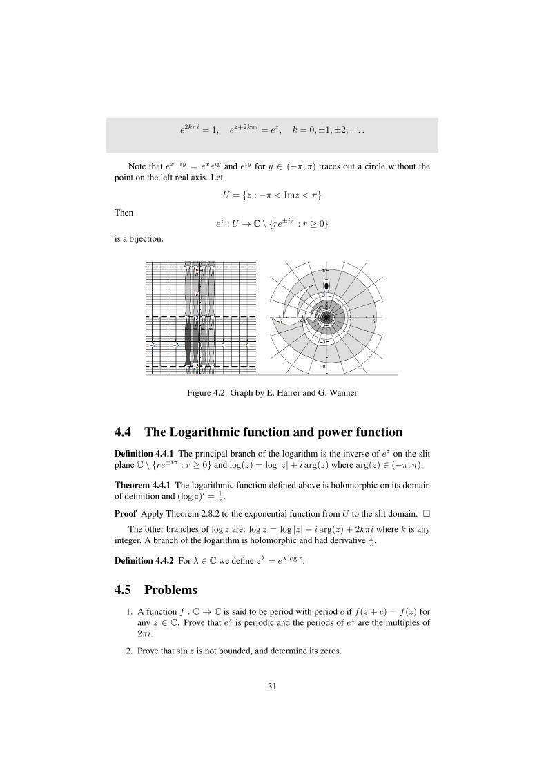
e2kπi = 1, ez+2kπi = ez, k = 0,±1,±2, . . . .

Note that ex+iy = exeiy and eiy for y ∈ (−π, π) traces out a circle without thepoint on the left real axis. Let

U = {z : −π < Imz < π}

Thenez : U → C \ {re±iπ : r ≥ 0}

is a bijection.

Figure 4.2: Graph by E. Hairer and G. Wanner

4.4 The Logarithmic function and power functionDefinition 4.4.1 The principal branch of the logarithm is the inverse of ez on the slitplane C \ {re±iπ : r ≥ 0} and log(z) = log |z|+ i arg(z) where arg(z) ∈ (−π, π).

Theorem 4.4.1 The logarithmic function defined above is holomorphic on its domainof definition and (log z)′ = 1

z .

Proof Apply Theorem 2.8.2 to the exponential function from U to the slit domain. �

The other branches of log z are: log z = log |z| + i arg(z) + 2kπi where k is anyinteger. A branch of the logarithm is holomorphic and had derivative 1

z .

Definition 4.4.2 For λ ∈ C we define zλ = eλ log z .

4.5 Problems1. A function f : C → C is said to be period with period c if f(z + c) = f(z) for

any z ∈ C. Prove that ez is periodic and the periods of ez are the multiples of2πi.

2. Prove that sin z is not bounded, and determine its zeros.

31

Chapter 5

Complex integration

If a continuous function has a primitive in a region, then its integral along any closedpiecewise smooth curve vanishes. The converse holds in a star region (more generally,in a simply connected region): if a continuous function integrate to zero along anytriangle inside the region, then it has a primitive. Goursat’s theorem states that the in-tegral of a holomorphic function in a region indeed integrate to zero along any trianglewho and whose interior is contained in the region. From this we see Cauchy’s Theoremfor a star region: if f is holomorphic in a star region, then it integrates to zero alongany closed smooth curve γ whose interior is contained entirely in the region. Cauchy’sTheorem is in fact valid for any simply connected region.

Every point in a region U has a disc around it, contained entirely in U . So everypoint in U has a star region neighbourhood. In another word, a holomorphic functionintegrates to zero along any closed smooth curve with sufficiently small enclosure. Thedistinction between the local and the global null integral property relates to homotopytheory as well as to de Rham’s cohomology theory built on closed and exact differen-tial forms, both are related to the concept of ‘simply connectedness of a region’. Onthe complex plane, the simply connectedness can be explained visually (e.g. by theconformal mapping theorem) which is also responsible for the beauty of the theoryon the plane. It is perhaps confusing in the beginning when confronted with differentversion’s and various forms of Cauchy’s formulas, the rule of thumb is the following.That a function is differentiable at a point is a local property, we could pick our discas small as we like; a value for an integral along a closed curve is a global property: itdepends on the region enclosed by the curve.

5.1 Integration along curves (Lecture 7)Let z : [a, b] → C be a function, By z is differentiable at t ∈ (a, b) and has derivativez′(t) we mean that

z′(t) = limε→0

z(t+ ε)− z(t)ε

.

By z is differentiable at a and b we mean it has one sided derivatives. If z is dif-ferentiable with continuous derivative (with z′(t) 6= 0), we say that it is smooth. Apiecewise smooth curve consisting of a finite number of smooth pieces, joined at theends. We sometimes abbreviate ‘a piecewise smooth curve’ to ‘a smooth curve’.

32

Definition 5.1.1 A curve z : [a, b]→ C is piecewise smooth if z is continuous on [a, b]and there exist ti s.t. a = t0 < t1 < · · · < tn = b, s.t. z is smooth on each sub-interval[ti, ti+1].

Definition 5.1.2 The set {z(t) : a ≤ t ≤ b} is called the trace of the curve and isdenoted by {γ}.

Definition 5.1.3 Two parameterizations γ : [a, b] → C and γ′ : [a′, b′] → C areequivalent if there exists a C1 bijection φ : [a′, b′] → [a, b] such that φ′(t) > 0 andγ′ = γ ◦ φ.

A parameterized curve has an orientation: it is the direction in which a pointon the curve travels as the parameter t increases. The condition φ′(t) > 0 meansthat φ is strictly increasing and orientation is preserved. The family of all equivalentparameterizations determine an oriented curve.

We would be interested in the contour of a region, e.g. the contour of a disc is thecircle, traveled anticlockwise once. By a circle, we usually mean traveling along it,anti clockwise, once.

Example 5.1.1 1. The circle {|z − z0| = r} has the obvious parameterizations:

z = z0 + reiθ, 0 ≤ θ ≤ 2π.

The orientation of the curve is anticlockwise (it is a positively oriented curve).The curve

z = z0 + re−iθ, 0 ≤ θ ≤ 2π

is negatively oriented.

2. The curves z : [0, 1] → C with z(t) = 2t and z : [0, 2] → C with z(t) = t areequivalent. Take φ(t) = t/2 then z = z ◦ φ.

Definition 5.1.4 If γ is a smooth curve with parameterization z : [a, b] → C and f isa function continuous and defined on the trace of γ, then the (line) integral of f alongalong γ is ∫ b

a

f(z(t))z(t)dt.

This is also denoted by∫γf and

∫γf(z)dz.

Remark 5.1.2 The integral can be defined by by Riemann sums. Let ∆ : a = s0 <s1 < · · · < sn = b. Then∫

γ

f = lim|∆|→0

n−1∑k=1

f(z(s∗k))(z(sk)− z(sk−1)),

33

where s∗k ∈ [sk−1, sk] and |∆| = maxj |sj−sj−1| denotes the modulus of the partition.If f : [a, b] → C is a continuous function and f(t) = u(t) + iv(t) then its integral isgiven by the integral of its real and negative parts:∫ b

a

f(t)dt =

∫ b

a

u(t)dt+ i

∫ b

a

v(t)dt.

Example 5.1.3 Let z : [0, 2π] → C with z(t) = z0 + reit where r is a real numberand z0 ∈ C. The curve is the circle |z − z0| = r with positive orientation. Let n be aninteger. Then ∫

γ

(z − z0)ndz =

{0, n 6= −12πi, n = −1.

Proof ∫γ

(z − z0)ndz =

∫ 2π

0

(reit)nd

dt(reit)dt = rn+1i

∫ 2π

0

ei(n+1)tdt.

If n = −1, ∫γ

1

z − z0dz = i

∫ 2π

0

dt = 2πi.

If n 6= −1,∫γ

(z − z0)ndz = rn+1i

∫ 2π

0

[cos((n+ 1)t) + i sin((n+ 1)t)] dt = 0.

�

Proposition 5.1.4 Let γ : [a, b]→ C be a C1 curve and φ : [a′, b′]→ [a, b] a C1 non-decreasing function with φ(a′) = a and φ(b′) = b, then for any function continuouson {γ}, ∫

γ

f =

∫γ◦φ

f.

In particular, the integral∫γf(z)dz is independent of the (equivalent) parameterization.

Proof Let z : [a, b] → C and z : [a′, b′] → C be two parameterizations of γ. Letφ : [a′, b′]→ [a, b] be a C1 bijection such that α′(t) > 0 and z = z ◦ φ. Then∫

γ◦φf =

∫ b′

a′f(z(t))

d

dtz(t)dt =

∫ b′

a′f(z ◦ φ(t))

d

dtz(φ(t))dt

=

∫ b′

a′f(z ◦ φ(t))z(φ(t))φ(t)dt =

∫ b

a

f(z(s))z(s)ds.

�

Example 5.1.5 The curves γ given by z : [0, 2π] → C with z(t) = eit and the curveγ given by z : [0, 2π]→ C with z(t) = e2it are not equivalent. Indeed,

∫γ

1zdz = 2πi,

while∫γ

1zdz =

∫ 2π

0e−2it2ie2itdt = 4πi.

34

Definition 5.1.5 If γ is a piecewise smooth curve consisting of (a finite number of)smooth curves γi, we define∫

γ

f(z)dz =∑i

∫γi

f(z)dz.

Definition 5.1.6 The length of the curve γ is:

length(γ) =

∫ b

a

|z′(t)|dt.

By an argument similar to that in the proposition above, the length of the curve is alsoindependent of (equivalent) parameterization.

Theorem 5.1.6 The following properties hold.(1) For k1, k2 ∈ C,∫

γ

(k1f + k2g)(z)dz = k1

∫γ

f(z)dz + k2

∫γ

g(z)dz.

(2) If the curve γ has parameterization z : [a, b] → C, we define γ− to be the curve:z− : [a, b] → C given by z−(t) = z(a + b − t). This is the same curve with reversedorientation. Then ∫

γ

f(z)dz = −∫γ−f(z)dz.

(3) ∣∣∣∣∫γ

f

∣∣∣∣ ≤ supz∈{γ}

|f(z)| · length of (γ).

The proof is easy for the first two statements. The last one follows from the lemmabelow.

Lemma 5.1.7 ∣∣∣∣∣∫ b

a

f(t)dt

∣∣∣∣∣ ≤∫ b

a

|f(t)|dt.

Proof Let θ be the principle argument of the complex number∫ baf(t)dt. Then∣∣∣∣∣

∫ b

a

f(t)dt

∣∣∣∣∣ = e−iθ∫ b

a

f(t)dt =

∫ b

a

e−iθf(t)dt.

Since∫ bae−iθf(t)dt is a real number,∫ b

a

e−iθf(t)dt = Re

(∫ b

a

e−iθf(t)dt

)=

∫ b

a

Re(e−iθf(t)

)dt ≤

∫ b

a

|f(t)|dt.

�

35

Remark 5.1.8 Let us write f = u+ iv and z(t) = x(t) + iy(t). Then

f(z(t))z(t) = u(z(t))x(t)− v(z(t))y(t) + i (u(z(t))y(t) + v(z(t))x(t)) .

Hence ∫γ

f(z)dz =

∫ b

a

(u(x(t), y(t))x(t)− v(x(t), y(t))y(t)

)dt+

i

∫ b

a

(u(x(t), y(t))y(t) + v(x(t), y(t))x(t)

)dt.

5.2 Path independent property (Lecture 8)

Definition 5.2.1 A function f : U → C is said to have a primitive if there exists aholomorphic function F with F ′ = f .

The Fundamental theorem of Calculus states that if g : [a, b] → R is a continuousfunctions, then G′(x) = g(x) where G(x) =

∫ xag(t)dt. Unlike for real differentiabil-

ity, the existence of a primitive is a much stronger property. To begin with, given twopoints on a plane, there are many paths leading from one to the other and we would beinterested in a ‘path independent’ property. Later we see that if f has a primitive in aregion, it is itself complex differentiable in this region.

Rule of thumb. If you have a real valued function g of one variable x with explicitformulation which does not involve the number i, denote f the function obtained byreplacing x with z. Then f is a ‘candidate analytic continuation’ of g. One could firstcompute the formal anti-derivative of g and denote it by G. Now in G replace x by zand denote the function by F . Then F is a ‘candidate primitive’ for f . Once we havea primitive, check it out: is it actually complex differentiable in the desired region? Ifso, we can verify it is a primitive by the rules of differentiation.

Definition 5.2.2 A curve γ : [a, b]→ C is closed if γ(a) = γ(b).

Theorem 5.2.1 (path independendent property) Let U be an open set and f : U →C is continuous and has a primitive F . If z : [a, b] → U is a piecewise smooth curvewith initial point w1 and end point w2, then∫

γ

f = F (w2)− F (w1).

In particular, if γ is a closed curve then∫γ

f(z)dz = 0.

Proof We first assume that γ is smooth with parametrerization: z : [a, b]→ C.∫γ

f(z)dz =

∫ b

a

f(z(t))z′(t)dt =

∫ b

a

F ′(z(t))z′(t)dt

36

=

∫ b

a

d

dtF (z(t))dt = F (z(b))− F (z(a)) = F (w2)− F (w1).

If γ is a piecewise smooth curve, joined by smooth curves on each subinterval of t0 =a < t1 < · · · < tn = b, then we have a telescopic sum as following:∫

γ

f(z)dz

=[F (z(tn))− F (z(tn−1))] + · · ·+ [F (z(t2))− F (z(t1))] + [F (z(t1))− F (z(t0))]

=F (z(b))− F (z(a)) = F (w2)− F (w1).

�

Example 5.2.2 The circle C = {z : |z| = 1} is contained entirely in the disc D ofradius 2 with center 0. Since

∫C

1zdz = 2πi, 1

z has no primitive in D.

Example 5.2.3 Let γ be the upper circle C+ = {z : |z| = 1, Im(z) ≥} followed bythe line segment [−1,−2]. Then

∫γezdz = e−2 − e1.

Remark 5.2.4 If an open subset of C is connected, then any two points can be con-nected by a polygon (i.e. a continuous curve consists of a finite number of piecewiseline segments) whose line segments are parallel either to the real axis or parallel to theimaginary axis.

Corollary 5.2.5 If f : U → C is holomorphic, where U is open and connected, andf ′ vanishes identically on U then f is a constant.

Proof Let us fix a point z0 ∈ U . Let z ∈ U be any other point. Let γ be such a polygonconnecting z0 and z. Since f ′ = 0 is a continuous function,

0 =

∫γ

0dz = f(z)− f(z0),

concluding that f is a constant. �

5.3 Existence of primitivesThe converse to the vanishing of integral theorem is at the heart of complex integration,for which we must restrict the region. We work with a sub class of regions of the simplyconnected region, called the star regions.

Definition 5.3.1 A region U is said to be a star region if it has a centre C, by whichwe mean for all z ∈ U , the line segment from C to z (denoted by [C, z]),

{(1− t)C + tz : 0 ≤ t ≤ 1}

belongs to U .

37

Note that z(t) = (1− t)C + tz is a prameterization of the line segment from C toz.

Star regions include discs, triangles, rectangles and more generally convex sets. Astar region is simply connected, by which we mean any simple closed curve in thatregion can be continuously deformed to a point. Many regions such as polygons canbe divided into star regions, which allow us to conclude statements for star regions formore general regions.

Figure 5.1: Graph by E. Hairer and G. Wanner

Theorem 5.3.1 (Integrability Criterion) Let U be a star region with a centre C andf : U → C a continuous function such that∫

T

f(ζ)dζ = 0

for any triangle T , contained entirely in U , and with C as one of its vertex. Then

F (z) =

∫[C,z]

f(ζ)dζ, z ∈ U,

is a primitive of f .In particular,

∫γf = 0 for any closed piecewise smooth curve z : [a, b]→ U .

Proof For any z ∈ U , the line segment [C, z] is contained in U and we may defineF (z) =

∫[C,z]

f(ζ)dζ.Let z0 ∈ U we show that F ′(z0) = f(z0). Since U is open there exists δ0 such that

D(z0, δ0) is contained in U . Take z ∈ D(z0, δ0) then [z0, z] ∈ U . Since [C, z0] and[C, z] lies in U , the triangle with vertex z0, z and C is contained entirely in U . Denote

38

by T this triangle. By the assumption,∫T

f =

∫[C,z]

f +

∫[z0,z]

f −∫

[C,z0]

f = 0

The last equality holds also if z, z0, w are on the same line. Thus

F (z) = F (z0) +

∫[z0,z]

f.

Since f(z0)z is a primitive of f(z0),∫

[z0,z]f(z0)dζ = f(z0)(z − z0) and

F (z) = F (z0) + f(z0)(z − z0) +

∫[z0,z]

(f(ζ)− f(z0))dζ.

Define ψ(z0) = 0 and for z 6= z0,

ψ(z) =

∫[z0,z]

(f(ζ)− f(z0))dζ

|z − z0|.

By the continuity of f , for any ε > 0 there exists δ ∈ (0, δ0) such that if |z − z0| < δ,|f(z)− f(z0)| < ε. Then

|ψ(z)| =

∣∣∣∣∣∫

[z0,z](f(ζ)− f(z0))dζ

|z − z0|

∣∣∣∣∣ ≤ 1

|z − z0|ε · length([z0, z]) = ε.

This proves that F is differentiable at z0 with F ′(z0) = f(z0), since z0 is an arbitrarypoint in U , F is holomorphic in U and is a primitive of f . �

5.4 Goursat’s Lemma and Cauchy’s Theorem for starregions

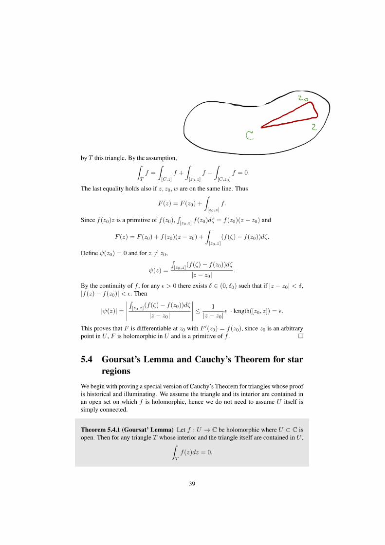
We begin with proving a special version of Cauchy’s Theorem for triangles whose proofis historical and illuminating. We assume the triangle and its interior are contained inan open set on which f is holomorphic, hence we do not need to assume U itself issimply connected.

Theorem 5.4.1 (Goursat’ Lemma) Let f : U → C be holomorphic where U ⊂ C isopen. Then for any triangle T whose interior and the triangle itself are contained in U ,∫

T

f(z)dz = 0.

39

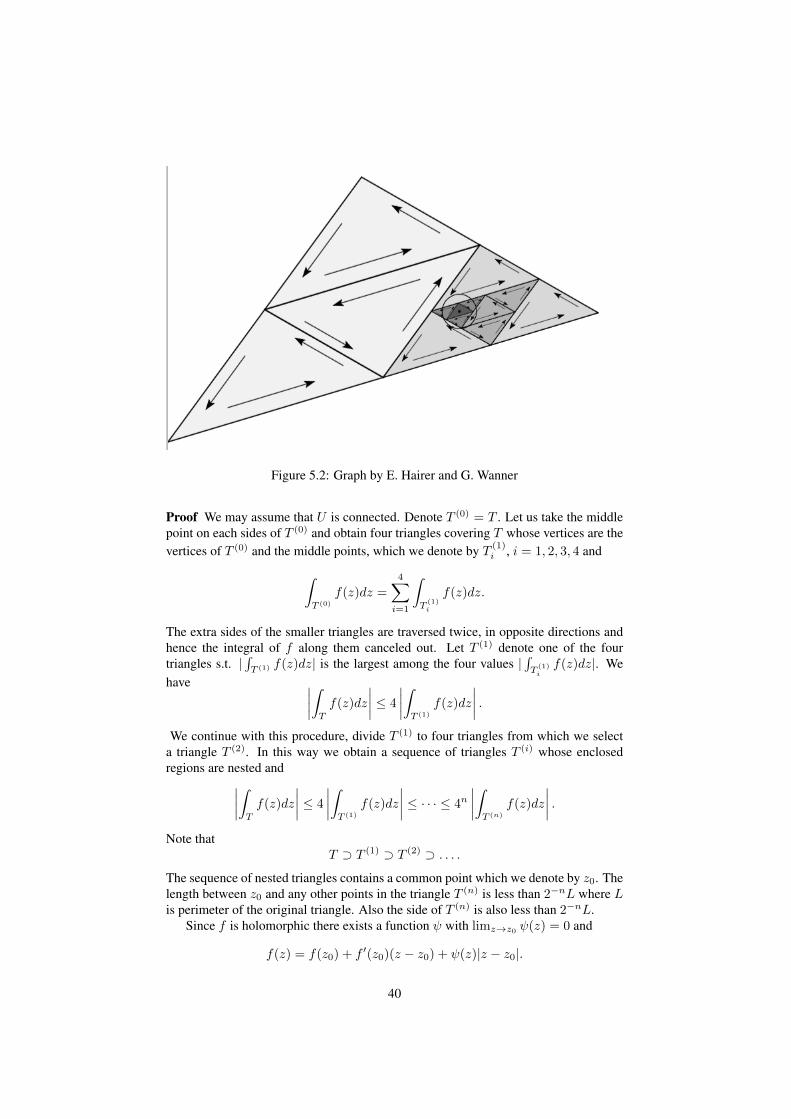
Figure 5.2: Graph by E. Hairer and G. Wanner

Proof We may assume that U is connected. Denote T (0) = T . Let us take the middlepoint on each sides of T (0) and obtain four triangles covering T whose vertices are thevertices of T (0) and the middle points, which we denote by T (1)

i , i = 1, 2, 3, 4 and∫T (0)

f(z)dz =

4∑i=1

∫T

(1)i

f(z)dz.

The extra sides of the smaller triangles are traversed twice, in opposite directions andhence the integral of f along them canceled out. Let T (1) denote one of the fourtriangles s.t. |

∫T (1) f(z)dz| is the largest among the four values |

∫T

(1)if(z)dz|. We

have ∣∣∣∣∫T

f(z)dz

∣∣∣∣ ≤ 4

∣∣∣∣∫T (1)

f(z)dz

∣∣∣∣ .We continue with this procedure, divide T (1) to four triangles from which we select

a triangle T (2). In this way we obtain a sequence of triangles T (i) whose enclosedregions are nested and∣∣∣∣∫

T

f(z)dz

∣∣∣∣ ≤ 4

∣∣∣∣∫T (1)

f(z)dz

∣∣∣∣ ≤ · · · ≤ 4n∣∣∣∣∫T (n)

f(z)dz

∣∣∣∣ .Note that

T ⊃ T (1) ⊃ T (2) ⊃ . . . .

The sequence of nested triangles contains a common point which we denote by z0. Thelength between z0 and any other points in the triangle T (n) is less than 2−nL where Lis perimeter of the original triangle. Also the side of T (n) is also less than 2−nL.

Since f is holomorphic there exists a function ψ with limz→z0 ψ(z) = 0 and

f(z) = f(z0) + f ′(z0)(z − z0) + ψ(z)|z − z0|.

40

Since f(z0)+f ′(z0)(z−z0) has a primitive its integral along any closed curve vanishes.Hence ∫

T (n)

f(z)dz =

∫T (n)

ψ(z)|z − z0|dz.

Since |z − z0| ≤ 2−nL and

4n∣∣∣∣∫T (n)

f(z)dz

∣∣∣∣ ≤ 4nlength(T (n))2−nL maxz∈T (n)

|ψ(z)| ≤ 4n(2−nL)2 maxz∈T (n)

|ψ(z)| → 0.

Consequently,∫Tf(z)dz = 0. �

Goursat (1884) actually proved the above for rectangles by sub-dividing rectangles.

Remark 5.4.2 Suppose that f is holomorphic in a region U , then for any rectangle Rwho and whose interior contained entirely in U ,∫

R

f(z)dz = 0

Proof Just divide R into two triangles T1 and T2 whose share a side which are trans-versed twice in opposite directions. Hence∫

R

f(z)dz =

∫T1

f(z)dz +

∫T2

f(z)dz.

�

A similar proof shows that in Goursat’s theorem we may replace the triangle byany polygons. Argue by induction on the number of sides in a polygon, once see thatGoursat’s theorem holds for polygons.

Theorem 5.4.3 (Cauchy’s Theorem, existence of primitive) A holomorphic functionon a disc {z : |z − C| < r} has

F (z) =

∫[C,z]

f(ζ)dζ

as its primitive.In particular, if γ : [a, b]→ D is a closed curve,∫

γ

f(z)dz = 0.

Proof Since U is a disc, the interior of a triangle lie in U if the triangle lie in U .Goursat’s Lemma states that

∫Tf(z)dz = 0 for any triangle who and whose interior

lie in U . By Theorem 5.3.1, F is a primitive of f and∫γf = 0 for any piecewise

smooth curve γ : [a, b]→ U . �

We will see that Cauchy’s Theorem extends to simply connected regions.

41

5.5 Integration along homotopic curvesTwo closed continuous curves γ0, γ1 curves are homotopic to each other if one canbe continuously deformed into the other. By re-parameterisation, we may assume thatboth curves are defined on [0, 1].

The precise meaning of the continuous deformation is as the following.

Definition 5.5.1 Let U be an open set. Let γ0, γ1 : [0, 1] → U be closed piecewisesmooth curves. We say that γ0 and γ1 are homotopic in U , denoted by γ0 ∼ γ1, if thereexists a continuous map F (s, t) : [0, 1]× [0, 1]→ U such that

F (s, 0) = γ0(s), F (s, 1) = γ1(s, 1), ∀s ∈ [0, 1]

and such that F (0, t) = F (1, t) for all t ∈ [0, 1].

In other words F defines a family of curves γt : [0, 1] → U which begins with γ0

and ends with γ1.

Theorem 5.5.1 If γ0 and γ1 are two closed piecewise smooth curves in a region U andγ0 ∼ γ1 in U . Then

∫γ0f =

∫γ1f for any holomorphic function f on U .

Proof Let Γ : [0, 1] × [0, 1] be the continuous function defined earlier. The graphof G is a compact set in U and hence its distance, which we denote by r, from thecomplement of U is positive. Since Γ is uniformly continuous there exists a naturalnumber n such that if (s− s′)2 + (t− t′)2 < 1

4n2 then, Γ(s, t)− Γ(s′, t′) < r.Let us subdivide [0, 1]× [0, 1] into n2 squares of equal size and denote by

Jjk =

[j

n,k

n

]×[j + 1

n,k + 1

n

]be one of the n2 squares. Denote the image of the vertex ( jn ,

kn ) by Zjk:

Zj,k = Γ(j

n,k

n),

and Pjk the polygon connecting Zj,k, Z(j+1),k, Zj+1,k+1 and Zj+1,k. Then

Pjk ⊂ B(Zj,k, r)

and so by Cauchy’s Theorem for a disc,∫Pjk

f = 0,

for any holomorphic functions f .Let us denote byQk the closed polygon which consists of line segments connecting

the following points Z0,k, Z1,k, . . . , Zn,k, observing that P0,k = Zn,k. We will provethat ∫

γ0

=

∫Q0

=

∫Q1

f = · · · =∫Qn

f =

∫γ1

f.

42

Let σj denotes the part of the curve on γ0 connecting Zj,0 to Zj+1,0. Let it befollowed by the line segment from Zj+1,0 back to Zj,0. This is a closed curve within adisc. Hence its integral vanishes and∫

σj

f =

∫[Zj,0,Zj+1,0]

f.

Summing up over j we recover the integral over γ0 and over Q0 respectively and con-clude that ∫

γ0

f =

∫Q0

f.

Similarly, ∫γ1

f =

∫Qn

f.

To prove that∫Qkf =

∫Qk+1f

, we note that

∑j

∫Pjk

f = 0.

These squares consists of the line segments from Qk and Qk+1 respectively, and in-tegration along the adjacent line segments travelling vertically, i.e. along Zj,k andZj,k+1, come in pairs and travel in the opposite directions. Rearrange the remainingterms we have

∫Qkf =

∫Qk+1f

. This completes the proof that∫γ0f =

∫γ1f .

�

Definition 5.5.2 We say that γ is homotopic to 0, γ ∼ 0, if γ is homotopic to a constantcurve.

Definition 5.5.3 A connected set is simply connected if any rectifiable curve is homo-topic to 0.

We will not discuss rectifiable curve, only need to know that a piecewise smoothcurve is a rectifiable curve. In a simply connected domain, any piecewise smooth curvecan be continuously deformed into a point.

Theorem 5.5.2 (Cauchy’s Theorem, c.f. Theorem 5.4.3) Let U be a simply con-nected region and f : U → C be holomorphic. Then for any closed (piecewise smooth)curve γ in U ,

∫γf = 0. Furthermore f has a primitive.

Remark 5.5.3 A star region is simply connected. They include convex sets and mostimportantly discs. The strip {x+ iy : 1 < x < 2} is simply connected.

43

Remark 5.5.4 A region in C is simply connected if and only if its complement in theextended plane C is connected. A bounded region in C is simply connected if and onlyif its complement in C is connected.

A simple curve is a curve which does not intersect itself.

Lemma 5.5.5 (Jordan curve theorem) The graph of a a simple closed curve dividesthe complex plane into two connected components, one of which is bounded and theother unbounded. The bounded is called the interior, the other is the exterior.

Whenever a closed simple curve lies in a simply connected region, its interior lies alsoin the region. If U is a region, it is easy to spot a subset of C \ U that is a positivedistance from the rest. Such subsets are ‘holes’ in U .

It is much easier to describe a curve as the boundary of a region (the contour).The boundary curve of a region are not necessarily smooth. We only consider contourcurves that are piecewise smooth and oriented positively, so the enclosed region stayson its left as we travel in the positive direction along the boundary. If U is a region theboundary curve of U is denoted by ∂U .

The following are non-simply connected regions:

{z : r1 < |z − z0| < r2}, {z : 0 < |z − z0| < r2}

Also, not simply connected:

{|z| < 20} \ {{|z − i| < 2} ∪ {|z − 1| < 1}}.

We are forced to consider non simply connected domains if a function has singularities.

Definition 5.5.4 A point z0 is an isolated singularity of f if f is holomorphic in somepunctured disk {0 < |z − z0| < r}, not differentiable or not defined at z0.

The function f(z) = 1z has an isolated singularity at 0.

Example 5.5.6 The function 1sin z has singularities at nπ where n ∈ Z.

For this we need to check the function sin(z) = 0 at and only at z = nπ. Firstlyusing the formula sin(z) = eiz−e−iz

2i we see that

sin(x+ iy) = sinx cosh y + i cosx sinh y

where cosh z = ez+e−z

2 and sinh z = ez−e−z2 . So sin(z) vanishes if and only if

sinx cosh y = 0, cosx sinh y = 0.

Since cosh y > 0 for y ∈ R, we have sinx = 0 and x = nπ. For x = nπ,cosx sinh y = ± sinh y which vanishes only if y = 0. Thus the zeros of sin z arenπ.

Example 5.5.7 f(z) =√z does not have an isolated singularity at 0. It cannot be

defined on any punctured disc around 0.

In the next chapter we discuss the integral of a function f along a contour curvewhich enclose an isolated singularity of f .

44

Chapter 6

Cauchy’s integral formula(Lecture 11)

If f is holomorphic in a region U then f has derivatives of all orders. Furthermore if z0

is such that a disc D centred at z0 is contained entirely in U , then it has a power seriesexpansion around z0 on D. Furthermore,

f (n)(z0) =n!

2πi

∫|z−z0|=r

f(ζ)

(ζ − z0)n+1dζ.

This is intimately related to the properties of the function 1z−z0 . For r > 0 denote

D(z0, r) = {z : |z − z0| < r}, C(z0, r) = {z : |z − z0| = r},

the latter is the curve γ(t) : [0, 2π]→ C with γ(t) = z0 + reit.

6.1 Cauchy’s integral formula

Lemma 6.1.1 Suppose thatD(w, ε) ⊂ D(z0, r). If f is holomorphic inU \{w}whereU is an open set containing D(z0, r) then∫

C(z0,r0)

f =

∫C(w,ε)

f.

Proof Let us draw a line passing z0 and w, this splits the two circles, the line segmentswill be denoted by Γ1,Γ2. The half circles are labelled C+

r , C−r , and C+

ε , C−ε . Thenthe region with boundary C+

r ∪Γ1 ∪Γ2 ∪−C+ε is contained in a slightly larger simply

connected region on which f is holomorphic. Hence f integrates to zero along thecontour. ∫

C+r

f +

∫Γ1

f +

∫Γ2

f −∫C+ε

f = 0.

Similarly, ∫C−r

f −∫

Γ1

f −∫

Γ2

f −∫C+ε

f = 0.

45

Add these two identities to obtain the required identity. �

Example 6.1.2 For any z0, w0 ∈ C and r > 0,∫C(w0,r)

1

z − z0dz =

{2πi, z0 ∈ D(w0, r);

0, z0 6∈ D(w, r).

If z0 ∈ D(w0, r), choose ε > 0 withD(z0, ε) ⊂ D(w0, r). Since 1z−z0 is holomor-

phic on D(w0, r) \ {z0}, by Lemma 6.1.1,∫C(w0,r)

1z−z0 dz =

∫C(z0,ε)

1z−z0 dz = 2πi.

If z0 6∈ D(w, r), choose ε > 0 so thatD(z0, ε)∩D(w, r) =. Then 1z−z0 is holomorphic

on D(w0, r′) for soem r′ > r. Then

∫C(w0,r)

1z−z0 dz = 0.

Theorem 6.1.3 (Cauchy’s Integral formula) Suppose that f is holomorphic onD(z0, R). Then for any 0 < r < R and any z ∈ C(z0, r),

f(z) =1

2πi

∫C(z0,r)

f(w)

w − zdw.

Proof Let ε be sufficiently small so D(z, 2ε) ⊂ D(z0, r). Then by Lemma 6.1.1,∫C(z0,r)

f(w)

w − zdz =

∫C(z,ε)

f(w)

w − zdw

=

∫C(z,ε)

f(w)− f(z)

w − zdz +

∫C(z,ε)

f(z)

w − zdw

=

∫C(z,ε)

f(w)− f(z)

w − zdw + f(z)2πi.

Since f is holomorphic, f(w)−f(z)w−z is bounded by a numberM onD(z, 2ε)\{z}. Thus∣∣∣∣∣

∫C(z,ε)

f(w)− f(z)

w − zdw

∣∣∣∣∣ ≤M · length(C(z, ε))→ 0, as ε→ 0.

Finally∣∣∣∣∣∫C(z,r)

f(w)

w − zdw − f(z)2πi

∣∣∣∣∣ ≤ lim supε→0

∣∣∣∣∣∫C(z,ε)

f(w)− f(z)

w − zdw

∣∣∣∣∣ = 0,

completing the proof. �

The value of a holomorphic function in a disc is determined by its values on theboundary circle.

Corollary 6.1.4 (Cauchy’s Integral formula for a disc) If f is holomorphic onD(z0, R)then for every 0 < r < R,

f(z0) =1

2π

∫ 2π

0

f(z0 + reit)dt.

46

Example 6.1.5 Let |a| > 1 and |b| < 1. Compute∫C(0,1)

1

(z − a)3(z − b)dz.

Set f(z) = 1(z−a)3 which is holomorphic on a disc D(0, r) where r ∈ (a, b). Then∫

C(0,1)

1

(z − a)3(z − b)dz =

∫C(0,1)

1

z − bf(z)dz = 2πif(a) = 2πi

1

(b− a)3.

6.2 Taylor expansion, Cauchy’s derivative formulas (Lec-ture 12)

Lemma 6.2.1 Let γ be a piecewise smooth curve, fn and f be continuous functionson {γ}, the trace of γ. Suppose that fn converges uniformly to f on {γ}, then∫

γ

fn =

∫γ

f.

Proof For any ε > 0 there exists N such that for n > N , |fn(w)− f(w)| < ε

length(γ)

for any w ∈ {γ}. Hence∣∣∣∣∫γ

fn −∫γ

f

∣∣∣∣ =

∣∣∣∣∣∫ b

a

[fn(γ(t))− f(γ(t))]γ′(t)dt

∣∣∣∣∣ ≤ ε

length (γ)· length(γ) = ε,

completing the proof. �

Theorem 6.2.2 (Taylor’s Theorem) If f is holomorphic on an open disc D(z0, R) ={z : |z − z0| < R}, then there exists a sequence of complex numbers an such that

f(z) =

∞∑n=0

an(z − z0)n, z ∈ D(z0, R).

In particular if f is holomorphic on an open set, it is analytic. Furthermore, for any0 < r < R,

an =f (n)(z0)

n!, an =

1

2πi

∫|w−z0|=r

f(w)

(w − z0)n+1dw.

Proof Let z ∈ D(z0, R). Choose a number r between |z − z0| and R. By Cauchy’sintegral formula, Corollary 6.1.4,

f(z) =1

2πi

∫|w−z0|=r

f(w)

w − zdw.

Now1

w − z=

1

(w − z0)− (z − z0)=

1

w − z0

1

1− z−z0w−z0

.

47

Since∣∣∣ z−z0w−z0

∣∣∣ = |z−z0|r < 1,

1

w − z=

1

w − z0

∞∑n=0

(z − z0)n

(w − z0)n

and ∫γ

f(w)

w − zdw =

∫γ

∞∑n=0

f(w)

(w − z0)n+1(z − z0)ndw.

On |w − z0| = r, |f | ≤M for a number M ,∣∣∣∣ f(w)

(w − z0)n+1

∣∣∣∣ ≤ M

rn+1.

Since∑∞n=0

|z−z0|nrn < ∞, by Weierstrass M -test, f(w)

(w−z0)

∑∞n=0

(z−z0)n

(w−z0)n convergesuniformly for w on the circle C(z0, r). By the earlier lemma,

f(z) =1

2πi

∫|w−z0|=r

f(w)

w − zdw =

∞∑n=0

(z − z0)n

an︷ ︸︸ ︷1

2πi

∫|w−z0|=r

f(w)

(w − z0)n+1dw .

By Theorem 4.2.2, an = f(n)(z0)n! . Also the series converge for |z− z0| < r for any

r < R and so the radius of convergence of the power series is at least R.Let U be an open set. If f : U → C is holomorphic, for any z0 ∈ U , h is

holomorphic on a disc containing z0, on which we just proved it has a Taylor seriesexpansion. Hence f : U → C is analytic. (c.f. Theorem 4.2.2). �

Corollary 6.2.3 (Cauchy’s derivative formula) If f is holomorphic onD(z0, R), thenfor any r ∈ (0, R),

f (n)(z) =n!

2πi

∫C(z0,r)

f(w)

(w − z)n+1dw, ∀z ∈ D(z0, R)

where C(z0, r) is the curve eit, t ∈ [0, 2π].

Proof The formula comes from the proof of Taylor’s Theorem and Lemma 6.1.1. �

Remark 6.2.4 Suppose that f : U → C is holomorphic, which does not admit ananalytic continuation to a larger open set. Let r be the distance from z0 to U . ThenD(z0, r) ⊂ U and f has a power series expansion with radius of convergence at leastr. In other words, if f is holomorphic in an open set including z0, it has a power seriesexpansion on a disc around z0, which is not the whole complex plane, must meet apoint where f is not differentiable (singularity).

6.3 Morera’s TheoremCorollary 6.3.1 (Morera’s Theorem) If f is continuous in a disc D and s.t.∫

T

f(w)dw = 0

for any triangle T contained in this disc, then f is holomorphic.

48

Proof By the integrability criterion, Theorem 5.3.1, there exists a holomorphic func-tion F such that F ′ = f . By Taylor’s theorem, f = F ′ is differentiable. �

6.4 Cauchy’s inequality, and Liouville’s TheoremTheorem 6.4.1 (Cauchy’s Inequality) If f is holomorphic in {z : |z − z0| < R},letting M = supz∈D(z0,R) |f(z)|, then

|f (n)(z0)| ≤M n!

Rn.

Proof Let r < R. By Cauchy’s derivative formula, or z ∈ D(z0, r),

|f (n)(z) =

∣∣∣∣∣ n!

2πi

∫C(z0,r)

f(w)

(w − z)n+1dw

∣∣∣∣∣≤ n!

2π

M

rn+1length(C(z0, r)) =

n!M

rn.

Since this holds for any r < R, we take r → R to obtain the required estimate. �

If f(z) =∑∞n=0 an(z − z0)n on D(z0, R), then

|an| =f (n)(z0)

n!≤ M

Rn.

Corollary 6.4.2 (Liouville’s Theorem) A bounded entire function is a constant.

Proof Let |f |∞ = supz∈C |f(z)|. By Cauchy’s inequality, for any z0, and any R,

|f ′(z0)| ≤ |f |∞1

R.

Taking R to infinity to see that f ′(z0) = 0. Since z0 is an arbitrary point in C, f ′

vanishes identically and f is a constant (by Corollary 5.2.5). �

Example 6.4.3 Since sin(z) is an entire function, by Liouville’s Theorem it cannotbe bounded on C, a fact can also easily be deduced from the formula sin(x + iy) =

sinx ey+e−y

2 + i cosx ey−e−y

2 .

An extension to Liouville’s Theorem is:

Example 6.4.4 If f is an entire function with limz→∞f(z)z = 0, then f is a constant.

Proof Let z0 ∈ C, R > 0. By Cauchy’s derivative formula,

f ′(z0) =1

2πi

∫|w−z0|=R

f(w)

(w − z0)2dw =

1

2π

∫ 2π

0

f(z0 +Reit)

Reitdt.

Hence

|f ′(z0)| ≤ 1

2π

∣∣∣∣∫ 2π

0

f(z0 +Reit)

z0 +Reitz0 +Reit

Reitdt

∣∣∣∣ ≤ sup0≤t≤2π

∣∣∣∣f(z0 +Reit)

z0 +Reit

∣∣∣∣ |z0|+R

R.

The right hand side converges to 0 as R → ∞. Hence f ′ = 0 identically and f is aconstant. �

49

Example 6.4.5 Let f be an entire function such that there exist real numbersR andMsuch that |f(z)| ≤M |z|n outside of the disc {z : |z| ≤ R}. Then f is a polynomial ofdegree at most n.

Proof An entire function f has a power series expansion at 0:

f(z) =

∞∑n=0

anzn, z ∈ C.

For m > n, and for any r > R,

|am| =1

2πi

∣∣∣∣∣∫|z|=r

f(z)

zm+1dz

∣∣∣∣∣ =1

2πi

∣∣∣∣∣∫|z|=r

f(z)

zn1

zm+1−n dz

∣∣∣∣∣≤ sup|z|=r

|f(z)||zn|

1

rm+1−n (2πr)→ 0,

as r →∞. Thus am = 0 for all m ≥ n and f is a polynomial of at most degree n. �

50

Chapter 7

Analytic Functions

In this chapter we use Cauchy’s Theorems to study properties of analytic functions.

7.1 Schwartz Reflection Principle (Lecture 13)Schwartz Reflection Principle is a method for extending a holomorphic function overand to the other side of the real axis.

Let U be an open subset of C, symmetric with respect to the real axis, i.e.

z ∈ U iff z ∈ U.

Let I = U ∩ R,

U+ = {z ∈ U, Im(z) > 0}, U− = {z ∈ U, Im(z) < 0}.

Then U = U+ ∪ I ∪ U−.

Theorem 7.1.1 (Symmetry Principle) If f+ and f− are respectively holomorphicfunctions on U+ and U−, that extends continuously to I , and f+(x) = f−(x) forany x ∈ I , define

f(z) =

f+(z), z ∈ U+

f+(z) = f−(z), z ∈ If−(z), z ∈ U−.

Then f is holomorphic on U .

Proof It is clear that f is continuous on U , holomorphic on U+ and on U−. Let z0 ∈ Iand D a disc in U centred at z0. Let T be a triangle in D we prove that

∫Tf(z)dz = 0.

There are three possibilities:

(a) T lies entirely within U+ or entirely within U−, then∫Tf(z)dz = 0 by Gour-

sat’s Lemma.

(b) One side of T is on I . For example assume T is in U+ ∪ I , in this case we take atriangle Tε by moving its side on I upward, horizontally, with its distance fromI to be ε. Then Tε → T and∫

Tε

f(z)dz →∫T

f(z)dz = 0.

By part (a),∫Tεf(z)dz vanishes for any ε, hence

∫Tf(z)dz = 0.

51

(c) T lies cross I in this case we may divide the triangles, T1 lies entirely on side ofthe I axis, each of the other triangles T2 and T3 have one side on I . By part (a)and (b),

∫Tif(z)dz = 0 for i = 1, 2, 3 and

∫T

f(z)dz =

3∑i=1

∫T

f(z)dz = 0.

We apply Morera’s Theorem to conclude that f is holomorphic on D. Since z0 is anaribitary point in I , f is holomorphic at each point of I . �

The following Lemma is given in Example Sheet 1.

Theorem 7.1.2 (Schwartz Reflection Principle) Suppose f is a holomorphic func-tion on U+ extending continuously to I , and f takes real value on I . Then there existsa holomorphic function F on U such that F and f agree on U+ ∪ I .

Proof We define

F (z) =

f(z), z ∈ U+ ∪ I

f(z) z ∈ U−.

For z ∈ I , F (z) = F (z) and so the function is well defined. We have seen that ifg : U− → C given by g(z) = f(z) is holomorphic. By the reflection principle, F isholomorphic on U . �

There are two proof for the complex differentiability of g : U− → C given byg(z) = f(z) where f is holomorphic on U+. Proof 1. (On Example sheet 1) Letz0 ∈ U− and z ∈ U−. Since f is differentiable in z0, there exists a function ψ withlimζ→z0 ψ(ζ) = 0 and

f(z) = f(z0) + f ′(z0)(z − z0) + ψ(z)|z − z0|.

Taking conjugate of both side we see that

g(z) = g(z0) + f ′(z0)(z − z0) + ψ(z)|z − z0|.

Since limz→z0 ψ(z) = 0 this proves that g is complex differentiable at z0 and g′(z0) =f ′(z0).

Proof 2. Let z0 ∈ U−. We make a Taylor expansion of f at z0 around a disc Dcontained in U+:

f(z) =

∞∑n=0

an(z − z0)n.

Then taking conjugate of both sides we see

g(z) =

∞∑n=0

an(z − z0)n,

hence g is analytic on U−.

52

7.2 Locally uniform convergence (Lecture 14)The limit of a sequence of continuous functions, converging uniformly, is continuous.Continuity is a concept which is the same weather we treat f as a complex valuedfunction of one complex variable or as a R2 valued function of two real variables.

Definition 7.2.1 A sequence of holomorphic functions in an open connected set U issaid to converge locally uniformly, if they converge uniformly on every compact subsetof U . We also say fn converges uniformly on compacts.

Theorem 7.2.1 (The Uniform Convergence Theorem/Weierstrass Theorem) If fn isa sequence of holomorphic function on an open connected set U that converges locallyuniformly to a function f , then f is holomorphic.

Proof Let z0 ∈ U and D = D(z0, R) a disc with its closure contained entirely in U .By Goursat’s Lemma for holomorphic functions on a disc, for each n,∫

T

fn(z)dz = 0

for any triangle in D. Since fn → f uniformly on D, f is continuous on D. Further-more, by Lemma 6.2.1, ∫

T

fn(z)dz →∫T

f(z)dz

and the latter vanishes. By Morera’s Theorem, f is holomorphic on D(z0, R). Sincez0 is an arbitrary point in U , we may conclude that f is holomorphic. �

Theorem 7.2.2 If fn is a sequence of holomorphic function on an open connected setU that converges locally uniformly to a function f , then f ′n converges to f ′ convergeslocally uniformly.

Proof Let K be a compact subset of U . Then there exists δ > 0 such that for eachz ∈ K, the disc D(z, 3δ) is contained in U . Observe that the distance from K to U c isgreater or equal to 3δ.

There exist a finite number of zi ∈ K such that K ⊂ ∪Ni=1D(zi, δ). To provef ′n → f ′ uniformly on K, we only need to prove f ′n converges uniformly on every discD(z0, δ) where z0 ∈ K.

By Cauchy’s derivative formula applied to D(z0, 2δ),

f ′n(z) =1

2πi

∫C(z0,2δ)

fn(w)

(w − z0)2dw, z ∈ D(z0, δ)

f ′(z) =1

2πi

∫C(z0,2δ)

f(w)

(w − z0)2dw, z ∈ D(z0, δ).

For any ε > 0 there exists N s.t. for n > N ,

supz∈ ¯D(z0,2r)

|fn(z)− f(z)| ≤ 2εδ, z ∈ D(z0, 2δ).

53

Observe that |z − w| > δ for z ∈ D(z0, δ) and w ∈ D(z0, 2δ), and so

|f ′n(z)− f ′(z)| = 1

2π

∣∣∣∣∣∫C(z0,2δ)

fn(w)− f(w)

(w − z0)2dw

∣∣∣∣∣ ≤ 2δ1

δ22εδ ≤ ε, z ∈ D(z0, δ),

c.f. Theorem 5.1.6, proving that f ′n → f ′ uniformly on compact subsets of U . �

Theorem 7.2.3 Let U be a region in C and G : U × [0, 1]→ C a continuous functions.t. G(·, s) is holomorphic for each s ∈ [0, 1]. Then the function f(z) =

∫ 1

0G(z, s)ds

is holomorphic.

Proof We define a family of holomorphic functions:

fn(z) =

n∑k=1

∫ kn

k−1n

G(z,k

n)ds =

1

n

n∑k=1

G(z,k

n).

Let z0 ∈ U andD(z0, 2r) a disc in U . ThenG is uniformly continuous on the compactset D(z0, r). Indeed, for any ε > 0, there exists δ > 0 such that if |s − t| < δ,|G(z, s)−G(z, t)| < ε for all z ∈ D(z0, r). If n > 1

δ , and z ∈ D(z0, r)

|fn(z)− f(z)| =

∣∣∣∣∣n∑k=1

∫ kn

k−1n

(G(z,k

n)−G(z, s))ds

∣∣∣∣∣ < ε.

Hence fn → f converges uniformly on D(z0, r). By Theorem 7.2.1, f is holomorphicon D(z0, r). Since z0 is an arbitrary point of U , f is holomorphic in U . �

7.3 zeros of analytic functions

7.3.1 The Fundamental Theorem of AlgebraThe zero of a function f is a solution to f(z) = 0.

Lemma 7.3.1 Every non-constant polynomial p(z) = a0 + a1z + · · · + anzn has at

least one zero.

Proof Suppose that p(z) has no root then 1p(z) is an entire function. We only need to

prove it is bounded. A bonded entire function is a constant.The entire function 1

p(z) is certainly bounded on any compact set. At far away itconverges to zero and so is also bounded on C \K where K is a compact set.

Detail for boundedness of 1p(z) . Suppose an 6= 0 for n ≥ 1. If z 6= 0,

p(z)

zn= (

a0

zn+

a1

zn−1+ · · ·+ an−1

z) + an.

The first term converges to 0 as z →∞ and∣∣∣p(z)zn

∣∣∣ ≥ |an|2 for |z| sufficiently large and∣∣∣∣ 1

p(z)

∣∣∣∣ =|zn||p(z)|

1

|z|n≤ 2

|an|1

|z|n,

which converges to zero as z →∞. Hence 1p(z) is a bounded. �

54

Theorem 7.3.2 (The Fundamental Theorem of Algebra) Every polynomial p(z) =a0 + a1z + · · · + anz

n of degree n ≥ 1 has precisely n zeros in C. Furthermore ifz1, . . . , zn are the roots then

p(z) = an(z − z1)(z − z2) . . . (z − zn).

Proof By the previous lemma p(z) = 0 has at least one root, z1. Write z = (z−z1)+z1

and expand p(z) in z − z1. There exist b0, b1, . . . , bn such that

p(z) = b0 + b1(z − z1) + · · ·+ bn(z − z1)n.

Evaluate p(z) at z1 giving b0 = 0. Hence

p(z) = (z − z1)(b1 + b2(z − z1) + . . . bn(z − z1)n−1 = (z − z1)Q(z).

By induction on the degree of the polynomial, Q(z) = 0 has n− 1 roots and

p(z) = A(z − z1) . . . (z − zn).

The number A is the coefficients in front of zn and is hence an. �

7.3.2 Zeros of analytic functions (Lecture 15)zeros of analytic functions are useful for a number of reasons: they are closely relatedto poles of meromorphic functions; the uniqueness of analytic continuations, and thedistributions of eigenvalues of a dynamical system. Or simply one wants to count thezeros, e.g. that of the zeta function!

The humblest application is to know where are the zeros of the derivative of aholomorphic function, which is also a holomorphic function. c.f. The Inverse FunctionTheorem and Conformal Mappings.

Let pn(z) be a polynomial of degree n and z0 a zero of pn(z). Then there exists anatural number r and w1, . . . , wn−r, not equal to z0 such that

pn(z) = an(z − z0)r(z − w1) . . . (z − wn−r).

The holomorphic function h(z) = an(z−w1) . . . (z−wn−r) does not vanish in a disccontaining z0. Furthermore,

p′n(z) = pn(z)

(r

z − z0+

1

z − w1+ · · ·+ 1

z − wn−r

).

If r > 1 it is clear p′n(z0) = 0. If r = 1,

p′n(z) =

(anΠn−1

i=1 (z − wi) + pn(z)

(1

z − w1+ · · ·+ 1

z − wn−1

)),

and p′n(z0) = anΠn−1i=1 (z0 − wi) 6= 0.

By induction on r we conclude that if z0 is a zero, or order r, of pn(z) then thefollowing holds:

• For k = 0, 1, . . . , r − 1, p(k)n (z0) = 0 (the k th derivatives).

• p(r)n (z0) 6= 0.

55

• There exists a holomorphic function h such that h(z) 6= 0 on a discD containingz0 and

pn(z) = (z − z0)rh(z), z ∈ D.

A trivial function is one which vanishes identically. A non-vanishing function is afunction that does not vanish anywhere.

We prove a multiplicative statement for a general holomorphic function.

Lemma 7.3.3 Suppose that f is a holomorphic function in a region U with a zero atz0. There exists a neighbourhood D of z0 such that either f is identically zero on D orthere exists a unique non-vanishing holomorphic function h onD, and a unique naturalnumber k such that

f(z) = (z − z0)kh(z), ∀z ∈ D.We say that f has a zero of order k at z0, in brief ord(f, z0) = k.

Proof (1) Since f is holomorphic, it has a power series expansion at z0, on a discD = D(z0, r):

f(z) =

∞∑n=0

an(z − z0)n, ∀z ∈ D.

Firstly a0 = f(z0) = 0 by the assumption. Suppose that f does not vanish identicallyon D. Let k ≥ 1 be the first non-zero term in the power series expansion. Then

f(z) = (z − z0)kak

(1 + (z − z0)

∞∑n=k+1

anak

(z − z0)n−k−1

).

Define

h(z) = ak

(1 + (z − z0)

∞∑n=k+1

anak

(z − z0)n−k−1

).

There exists M such that

sup|z|≤r/2

∣∣∣∣∣∞∑

n=k+1

an(z − z0)n−k−1

∣∣∣∣∣ ≤M,

as the power series inside the modulus sign converges on D(z0, r/2) and is a con-tinuous function on the disc D. Let r = min(r/2, 1

2M ). Then h is holomorphicand does not vanish on the open disc {|z − z0| ≤ r}. (3) Uniqueness. Supposef(z) = (z − z0)kh(z) = (z − z0)k h(z). If k > k then h(z) = (z − z0)k−k h(z) andh(z0) = 0, which contradicts with the definition of h. Consequently, k = k, and alsoh = h. �

Remark 7.3.4 Let f be a holomorphic function on a region U . f has a zero at z0 ororder k ∈ N if and only if

k = inf{k : f (k)(z0) 6= 0}.

Firstly, f ′(z) = k(z−z0)k−1h(z)+(z−z0)kh′(z). If k = 1, f ′(z0) = h(z0) 6= 0.If k > 1, f ′(z0) = 0. Induction on the degree k,

f (j)(z) = k(k − 1) . . . (k − j + 1)(z − z0)k−jh(z) + (z − z0)k−j+1G(z)

for a holomorphic function G. Thus f (j)(z0) = 0 for any j < k and f (k)(z0) 6= 0.

56

Theorem 7.3.5 Let U be a region in C. If f is a holomorphic function on U with asequence of zeros’s zk ∈ U with an accumulation point in U , then f(z) is trivial.

In particular, if two holomorphic functions in a region agree on a set of points withan accumulation pint, they are identical.

Proof Let zk be a sequence of zeros of f with limit z0. By the continuity, f(z0) =limk→∞ f(zk) = 0. So there exists D(z0, r) where r > 0 such that f vanishes onD(z0, r), for otherwise it has no other zeros besides z0 contradicting with the fact thatz0 is an accumulation points of zk (Lemma 7.3.6). We proceed to prove that f isidentically zero on U .

Let V be the interior of the set of zeros of f . Then V is non empty, it contains z0,and is an open set by the construction. If {zn} is a sequence in V with an accumulationpoint w0 ∈ U , we already see that w0 ∈ V . This proves V is closed in U and open. Idid not show that V is connected, we will use the connectedness of U .

Thus U is the union of two open sets:

U = (U \ V ) ∪ V.

If U \V is not empty, U is the disjoint union of nonempty open sets, contradicting withthe fact that U is connected. Hence f is identically zero. �

Remark 7.3.6 If f is a holomorphic function with f(z0) = 0. Then there exists a discD(z0, r) on which either f vanishes identically or f has no other zeros.

Definition 7.3.1 A zero of f , z0, is said to be isolated if there exists an open disc Daround z0 such that f(z) 6= 0 for any z ∈ D \ z0.

Every zero of a holomorphic function is isolated unless f is trivial on a disc near z0.The multiplicative statement can now be strengthened as below.

Theorem 7.3.7 (multiplicative statement) Suppose that f is a non-trivial holomor-phic function in a region U and has a zero at z0. There exists a neighbourhoodD of z0,a unique non-vanishing holomorphic function h on D, and a unique natural number ksuch that

f(z) = (z − z0)kh(z), ∀z ∈ D.

Use Lemma 7.3.3 and note that f vanishes in a neighbourhood of z0 implies that f istrivial on U (by Theorem 7.3.5).

Definition 7.3.2 Suppose f is holomorphic on U . Let z0 be a point on the boundaryof U . We say f is analytically continuable at z0 if there exists a holomorphic functiong : U ′ → R where U ′ is an open set containing z0 such that g and f agree in U ∩ U ′.

Example 7.3.8 Suppose that f1 : U1 → C, f2 : U2 → C are holomorphic. If U1 ∩ U2

is connected and f1 = f2 on a sequence of point zk ∈ U1 ∩ U2 with a limit z0 s.t.zk 6= z0 for any k then f1 = f2 on U1 ∩ U2.

Example 7.3.9 Let f be a holomorphic function in a region U . Let V ⊂ U be a closedbounded subset of U . Then for any w ∈ C, {z ∈ V : f(z) = w} has a finite numberof elements or f is a constant on V .

57

Discussion. Are there nowhere continuable power series beyond it disc of conver-gence? This was discussed by Weirerstrass 1880, Poincare 1892. The natural bound-ary for

∑∞n=0 cnz

λn ( for class of complex numbers cn’s) is its circle of convergenceif limn→∞(n/λn) = 0 (sufficiency by Fabry (1897), necessity by Polya (1942)). Itwas proved by Hadamard (1892) that inf{λn+1

λn} > 1 is sufficient for the statement.

Emile Borel showed that ‘in general’ a Taylor series is not continuable across the circleof convergence. This is ‘logical’, imagine a power series with radius of convergenceone, evaluating it on the circle of radius one is equivalent to

∑ane

iθ, these are simplyFourier series. A continuous periodic function on [0, 2π] is not in general analytic.

The Lacunary function is:

f(z) =

∞∑n=1

z2n = z + z2 + z4 + z8 + . . . .

The radius of convergence of the power series is R = 1. The largest open set on whichit can be extended analytically is the unit disc. In fact it has singularity at all 2n throots of the unity. Since the singularity points on the unit circle is dense in the circle,it cannot be analytically continued from any point on the circle. (Any continuationcontains a disc).

7.3.3 Maximum Modulus Principle (Lecture 16)Theorem 7.3.10 Suppose that f is a non-constant holomorphic function on D(z0, R)where R > 0. Then there exists a point w0 ∈ D(z0, R) s.t. |f(w0)| > |f(z0)|.

Proof We may assume that f(z0) 6= 0. (If f(z0) = 0, there is a point w0 withf(w0) 6= 0 or f is identically 0.) By Cauchy’s formula, for any r ∈ (0, R),

f(z0) =1

2π

∫ 2π

0

f(z0 + reit)dt.

We divide the equation above by f(z0). Write ff(z0) = u+ iv, then

1 =1

2π

∫ 2π

0

(u(z0 + reit) + i(z0 + reit)

)dt.

Suppose that |f(z)| ≤ |f(z0)| on D(z0, R), then u2(z) + v2(z) ≤ 1, and∫ 2π

0

u(z0 + eit)dt = 2π.

Since |u| ≤ 1 and u is continuous, this can happen if and only if u is identically 1. (If|u(z0)| < 1 at one point there exists a real number m0 < 1 s.t. |u(z)| ≤ m0 on aninterval of length δ > 0 and

∣∣∣∫ 2π

0u(z0 + eit)dt

∣∣∣ ≤ (2π − δ) +m0δ < 2π.)Thus u ≡ 1 and v = 0 and f is a constant on any disc D(z0, r), where r < R and

so f is a constant on D(z0, R), concluding the proof. �

By Theorem Theorem 7.3.5 below, if f is holomorphic on a connected open set U ,and is a constant on a disc D(z0, r) ⊂ for some z0 and r > 0, then f is a constanton U . Hence if f is a non-constant function in an open connected set U , on any discD(z0, r) ⊂ U , there exists a point w0 ∈ D(z0, r) such that |f(w0)| > |f(z0).

58

Why the argument for proving Maximum Modulus Principle might fail for the in-fimum, inf |f(z)|? Think of the case w0 = 0! In fact if the function f never vanishes,we would have no problem, just apply the Maximum Modulus Principle to 1

f .

Corollary 7.3.11 If f is a holomorphic function on a disc D(z0, R) and f(z0) 6= 0.Then for all 0 < r < R there exists z such that |f(z)| < |f(z0)|.

Proof Since f(a) 6= 0, f does not vanish in a disc D(z0, r0), r0 < R then 1f(z)

is holomorphic on D(z0, r0). There exists a point z in the disc D(z0, r0) such that∣∣∣ 1f(z)

∣∣∣ > ∣∣∣ 1f(z0)

∣∣∣. �

Example 7.3.12 Let f be a not constant holomorphic function in a neighbourhood ofthe closed unit disk D := {z : |z| ≤ 1}. Assume that |f(z)| is constant on ∂D :={z : |z| = 1}. Then f must attain at least one zero in D.

Suppose |f(z)| = 0 on the unit circle, then |f(z)| = 0 inside the disc, by theMaximum Modulous Principle, and the assertion holds trivially. Suppose |f(z)| =a > 0 on the unit circle then |f(z)| is non-zero in a neighbourhood of the unit circle.Assume that f does not have a zero in D. Then 1

f is holomorphic in D := {z : |z| < 1}and continuous on D. Then the supremum and infimum of |f(z)| are attained on theboundary: supz∈D |f(z)| = infz∈D |f(z)| = a. Hence |f(z)| is a constant on thewhole disc. By the Maximum Modulus Principle this implies that f is constant.

59

Chapter 8

Laurent series and singularities

A series of the formb1z−1 + b2z

−2 + . . .

can be considered as a power series in 1z . Let R denote its radius of convergence R. If

R is finite number, the power series converge absolutely for z with |z| > 1R . As usual,

1∞ is interpreted as 0.

If this series is combined with an ordinary power series we have a general series ofthe form

∞∑n=−∞

anzn.

Definition 8.0.1 The series is said to converge, if both its positive power part∑∞n=0 anz

n

and negative power part∑−∞n=−1 anz

n are separately convergent.

Suppose that the positive part of the power series has a radius of convergence R2 > 0and the negative part of the power series converges when |z| > R1. If R1 < R2,they have a common region of convergence: R1 < |z| < R2. Conversely if f isholomorphic function in a region contains the annulus R1 < |z − z0| < R2, it has ageneral series expansion at z0:

f(z) =

∞∑n=−∞

an(z − z0)n.

This is called a Laurent series (development) for f .

8.1 Cauchy’s formula and Laurent series (16-17)A function f is said to have an isolated singularity at z0 if f is defined and differentiablein an neighbourhood of z0 except at z0 itself. Example. f(z) = 1

(z−z0)k, where k ∈ N ,

has a singularity at z0.

Lemma 8.1.1 Let g be a holomorphic in an open set U containing A = {z : r1 <|z − z0| < r2} where 0 < r1 < r2. Then∫

C(z0,r1)

g(z)dz =

∫C(z0,r2)

g(z)dz.

60

Proof It is clear that the two circles are homotopic. Define e.g.

F (s, t) = z0 + (1− t) r1 eis + t r2 e

is.

Apply Cauchy’s Theorem to conclude. �

Lemma 8.1.2 Let f be a holomorphic function on a disc D(z0, r). Define

g(z) =

{f(z)−f(z0)

z−z0 , z 6= z0

f ′(z0), z = z0.

Then g is holomorphic on D(z0, r). Write this function g as fz0 .

Proof As the quotient of two holomorphic functions, g is differentiable on D \ {z0}.We only need to prove g is differentiable at z0. Firstly, there is a Taylor series expansionfor the holomorphic function f in a neighbourhood of z0

f(z) = f(z0) + f ′(z0)(z − z0) +

∞∑n=2

an(z − z0)n.

Hence for z 6= z0,

g(z)− g(z0) =f(z)− f(z0)

z − z0− f ′(z0) =

∞∑n=2

an(z − z0)n−1.

Andg(z)− g(z0)

z − z0=

∞∑n=2

an(z − z0)n−2,

The right hand side, a holomorphic function, has a limit as z → z0 and g is differen-tiable at z0.

�

Lemma 8.1.3 (Cauchy’s Integral formula for the annulus) Let f be a holomorphicfunction in an open set containing the annulus A = {z : r1 < |z − z0| < r2} where0 < r1 < r2 <∞. Then for all z ∈ A,

f(z) =1

2πi

∫C(z0,r2)

f(w)

w − zdw − 1

2πi

∫C(z0,r1)

f(w)

w − zdw.

Proof Let z ∈ A. Take a disc D around z, which is completely contained in A. Thenf is holomorphic on D We define on A,

fz(w) =

{f(w)−f(z)

w−z , w 6= z

f ′(z), w = z.

Then fz is holomorphic on the annulus by Lemma 8.1.2. By Lemma 8.1.1,∫C(z0,r1)

fz(w)dw =

∫C(z0,r2)

fz(w)dw.

61

Consequently, ∫C(z0,r2)

f(w)

w − zdw −

∫C(z0,r1)

f(w)

w − zdw

=

∫C(z0,r2)

f(w)− f(z)

w − zdw +

∫C(z0,r2)

f(z)

w − zdw

−∫C(z0,r1)

f(w)− f(z)

w − zdw −

∫C(z0,r1)

f(z)

w − zdw

=

∫C(z0,r2)

fz(w)dw −∫C(z0,r1)

fz(w)dw

+ f(z)

∫C(z0,r2)

1

w − zdw − f(z)

∫C(z0,r1)

1

w − zdw

=f(z)

∫C(z0,r2)

1

w − zdw − f(z)

∫C(z0,r1)

1

w − zdw.

We observe further, c.f. Example 6.1.2,∫C(z0,r2)

1

w − zdw = 2πi,

∫C(z0,r1)

1

w − zdw = 0,

as z is outside of the circle of integrationC(z0, r1) in the first case, and inside the circleof integration D(z0, r2) in the second case. The conclusion follows. �

Let r1 < r < r2. If f is holomorphic on the entire disc D(z0, r2), then for z inthe annulus, f(w)

w−z is holomorphic in a disc containing D(z0, r1), its integral along thecircle |z − z0| = r1 is zero by Cauchy’s Theorem:

1

2πi

∫C(z0,r1)

f(w)

w − zdw = 0.

Theorem 8.1.4 Let r1, r2 be two real numbers with 0 ≤ r1 < r2 ≤ ∞. Suppose thatf is holomorphic in a neighbourhood of the annulus {z : r1 < |z − z0| < r2}. Thenthere exists a unique sequence of complex numbers an such that

f(z) =

∞∑n=−∞

an(z − z0)n, r1 < |z − z0| < r2.

For any r1 < r < r2, for each n,

an =1

2πi

∫C(z0,r)

f(ζ)

(ζ − z0)n+1dζ. (8.1.1)

Proof Let z ∈ {z : r1 < |z − z0| < r2}. Then by Lemma 8.1.3,

f(z) =1

2πi

∫C(z0,r2)

f(ζ)

ζ − zdζ − 1

2πi

∫C(z0,r1)

f(ζ)

ζ − zdζ.

By the same proof as in the proof for Cauchy’s Theorem on Taylor formula, c.f. Theo-rem 6.2.2, we expand 1

ζ−z to obtain a power series expansion for the first term

1

2πi

∫C(z0,r2)

f(ζ)

ζ − zdζ =

∞∑n=0

an(z − z0)n

62

where an is as in formula (8.1.1). We work on

− 1

2πi

∫C(z0,r1)

f(ζ)

ζ − zdζ.

We observe that

1

ζ − z=

1

(ζ − z0)− (z − z0)= − 1

z − z0

1

1− ζ−z0z−z0

.

Since r1 = |ζ − z0| < |z − z0|, we expand 1

1− ζ−z0z−z0

as a power series and obtain:

1

ζ − z= − 1

z − z0

∞∑n=0

(ζ − z0)n

(z − z0)n= −

∞∑n=1

(ζ − z0)n−1

(z − z0)n.

By the uniform convergence of the series on {z : r1 < |z − z0|} (see remark below),we may exchange the order of taking limit and summing up and obtain

− 1

2πi

∫C(z0,r1)

f(ζ)

ζ − zdζ =

∞∑n=1

(z − z0)−n1

2πi

∫C(z0,r1)

f(ζ)(ζ − z0)n−1dζ.

Let m = −n and

am =1

2πi

∫|ζ−z0|=r

f(ζ)

(ζ − z0)m+1dζ.

Note the integration is independent of the radius of the circle, where r1 < r < r2, toconclude the theorem.

To prove the uniqueness suppose that we have another sequence of numbers suchthat

f(z) =

∞∑n=−∞

bn(z − z0)n, r1 < |z − z0| < r2.

Thenf(z)

(z − z0)k=

∞∑n=−∞

bn(z − z0)n−k.

Integrate both sides on the circle C(z0, r), with r ∈ (r1, r2), the only non-zero contri-bution comes from the term bk−1/(z − z0) which is:∫

C(z0,r)

bk−1(z − z0)−1dz = 2πibk−1.

Consequently,

bk =1

2πi

∫C(z0,r)

f(z)

(z − z0)k+1dz.

�

Remark 8.1.5 Since the annulus and its closure are contained in contained in the re-gion on which f is holomorphic, by slightly enlarging the annulus we may also taker = r1 or r = r2 in (8.1.1).

63

Remark 8.1.6 Suppose that the power series function f(z) =∑∞n=0 bn(z − z0)n has

radius of convergence R > 0. Then g(z) =∑∞n=0 bn(z − z0)−n is convergent for

|z − z0| > 1R , and the convergence is uniform on any set |z − z0| ≥ 1

r for any r < R.Just note that g(z) = f( 1

z−z0 ).

Note that the radius of convergence for the positive part of the Laurent series, in Theo-rem 8.1.4, is greater or equal to r2, the negative part converges on |z − z0| > r1.

Example 8.1.7 Let

f(z) =1

(z − 1)(z − 3)=

1

2(

1

z − 3− 1

z − 1).

Develop the Laurent series for f on the following regions:

{|z| < 1}, {1 < |z| < 3}, {|z| > 3}.

We observe that z0 = 0 and

1

z − 1=

−∑∞n=0 z

n, |z| < 1∑∞n=1 z

−n, |z| > 1.

1

z − 3=

= − 1

3 ·1

1− z3= −

∑∞n=0 3−n−1zn, |z| < 3

1z ·

11− 3

z

=∑∞n=1 3n−1z−n, |z| > 3.

Hence on {|z| < 1}, where f is holomorphic,

f(z) =1

2

(−∞∑n=0

3−n−1zn +

∞∑n=0

zn

)=

1

2

∞∑n=0

(1− 3−n−1

)zn.

On {1 < |z| < 3},

f(z) =1

2

(−∞∑n=0

3−n−1zn −∞∑n=1

z−n

)= −1

2

∞∑n=1

z−n − 1

2

∞∑n=0

3−n−1zn.

On |z| > 3,

f(z) =1

2

( ∞∑n=1

3n−1z−n −∞∑n=1

z−n

)=

1

2

−1∑n=−∞

(3−n−1 − 1)zn.

Corollary 8.1.8 (Cauchy’s Inequality) The coefficients in the Lauren series expan-sion f(z) =

∑∞n=−∞ an(z − z0)n satisfies:

|ak| ≤ sup|z−z0|=r

|f(z)| 1

rk

for any r ∈ (r1, r2).

Proof Just use the formula

|ak| =

∣∣∣∣∣ 1

2πi

∫C(z0,r)

f(ζ)

(ζ − z0)k+1dζ

∣∣∣∣∣ ≤ 1

2πsup

|z−z0|=r|f(z)|

(1

r

)k+1

L

where L = 2πr is the length of the circle. The conclusion follows. �

64

8.2 Classification of isolated singularities (Lecture 18)Denote D′(z0, r) = {z : 0 < |z − z0| < r} the deleted disc. Such a disc is a deletedneighbourhood of z0.

A point z0 is an isolated singularity for f , if f is defined and holomorphic on adeleted disc D′(z0, R), in which case f has a Laurent series at z0:

f(z) =

∞∑n=−∞

an(z − z0)n, z ∈ D′(z0, R).

Definition 8.2.1 (1) If ak 6= 0 for an infinite number of negative integers, we say fhas an essential singularity at z0.

(2) If f(z) =∑∞n=−k an(z − z0)n where k is positive and a−k 6= 0 we say f has a

pole at z0 of order k.

(3) If f(z) =∑∞n=0 an(z − z0)n we say z0 is a removable singularity.

In case (3), we extend f to f by defining f(z0) = a0. The extended function isholomorphic, hence the terminology f has a removable singularity at z0.

Proposition 8.2.1 Suppose that f is holomorphic on D′(z0, R). Then the Laurentseries of f is of the form f(z) =

∑∞n=−k an(z − z0)n, where the leading constant

does not vanish, if and only if there exist three numbers a > 0, b > 0, and δ > 0 suchthat

a

|z − z0|k≤ |f(z)| ≤ b

|z − z0|k, z ∈ D′(z0, R). (8.2.1)

Proof If f(z) =∑∞n=−k an(z − z0)n, then

(z − z0)kf(z) = a−k + (z − z0)

∞∑n=−k+1

an(z − z0)n+k−1.

On a sufficiently small disc,∣∣(z − z0)

∑∞n=−k+1 an(z − z0)n+k−1

∣∣ ≤ 12 |a−k|, from

which (8.2.1) follows. Assume (8.2.1) holds. We study the coefficients in the Laurentexpansion

f(z) =

∞∑n=−∞

an(z − z0)n, z ∈ D′(z0, R).

By Cauchy’s inequality, for any δ > 0,

|an| ≤ sup|z−z0|=δ

|f(z)|δ−n ≤ bδ−k−n.

If −k > n then an vanishes and f(z) =∑∞n=−k an(z − z0)n. Also a−k 6= 0,

for otherwise limz→z0 |f(z)||z − z0|k = 0 contradicting with (8.2.1), completing theproof. �

Theorem 8.2.2 (Riemann’s theorem on removable singularity) Let f be a holomor-phic function on the deleted discD′(z0, R). Then f has a removable singularity at z0 ifand only if f is bounded in a deleted neighbourhood of z0 in which case limz→z0 f(z)exists in C.

65

Proof If z0 is a removable singularity, it extends to a holomorphic function on a discD(z0, δ), so is bounded on D(z0, δ/2). If f is bounded, Cauchy’s inequality showsthat for any m ≤ 1, |am| ≤ δ−m → 0 as δ → 0. Hence am = 0 for any negative m.

Suppose f(z) =∑∞n=0 an(z − z0)n. Define and extension of f by f(z0) = a0.

Then f is holomorphic on D(z0, R) and limz→z0 f(z) = a0. �

Theorem 8.2.3 Let f be a holomorphic function on the deleted disc D′(z0, R). The fhas a pole at z0 if and only if limz→z0 |f(z)| =∞.

Proof Suppose that f has a pole of order k, where k < 0. By (8.2.1), a|z−z0|k ≤ |f(z)|,

limz→z0 |f(z)| =∞.If limz→z0 |f(z)| = ∞, then for a number M > 0 and r > 0, |f(z)| ≥ M on

D′(z0, r). Set g(z) = 1f(z) . Then g is holomorphic and bounded on D′(z0, r). Fur-

thermore limz→z0 g(z) = 0, and so g extends the analytic continuation g on D(z0, r)with g(z0) = 0. By the multiplicative statement for a holomorphic function with azero, there exists a disc D(z0, δ), a nowhere vanishing h and a number k > 0 such thatg(z) = (z− z0)kh(z). Hence f(z) = (z− z0)−k 1

h(z) . Since h(z) 6= 0 for any z, thereexist numbers a > 0 and b > 0 such that a < | 1

h(z) | < b on a small disc around z0.Apply Proposition 8.2.1 to see that f has a pole of order k at z0. �

Remark 8.2.4 A holomorphic function f on D′(z0, R) has a pole of order k at z0 ifand only if there exists a holomorphic function on a disc D(z0, δ) with H(z0) 6= 0 s.t.

f(z) = (z − z0)−kH(z), z ∈ D′(z0, δ),

On the extended plane, a pole can be ‘removed’ by the inversion map z 7→ 1z−z0 .

An essential singularity cannot be removed by any inversion map.

Definition 8.2.2 If {zk} is a sequence of complex numbers, we say limk→∞ zk = ∞if limk→∞

1zk

= 0.

Theorem 8.2.5 (Casorati-Weierstrass) Let f be a holomorphic function on the deleteddisc D′(z0, R). Then f has an essential singularity at z0 if and only if limz→z0 f(z)

does not exist on the extended plane C. Also f has an essential singularity at z0 if andonly if the image f(D′(z0, r)) is dense in C, for all 0 < r < R.

Proof The equivalence of the first two follows from the characterisation of a removingsingularity by |f | is bounded near z0 and that of a pole by the the limit |f(z)| to beinfinity as z → z0.

If f(D′(z0, r) is dense in C, it is clear that limz→z0 f(z) does not exist on theextended plane C.

Let z0 be an essential singularity of f . Suppose that there exists r > 0 such thatthe image of D′(z0, r) by f is not mapped to a set D(w0, δ) where δ > 0. Define

g(z) =1

f(z)− w.

Then g is holomorphic and bounded by 1δ onD′(z0, r). By Theorem 8.2.2, limz→z0

1g(z)

exists. If the limit vanishes, limz→z0 |f(z)| = limz→z0

∣∣∣w0 + 1g(z)

∣∣∣ = ∞ and z0 is a

66

pole. If g(z0) 6= 0 then

limz→z0

f(z) = w + limz→z0

1

g(z)

exists, then z0 would be a removable singularity for f ! We concluded that f(D(z0, r))must be dense in C. �

Example 8.2.6 The function f(z) = e1z has an essential singularity at z = 0. Check

that this function has no limit as z → 0.

8.2.1 Poles and ResiduesDefinition 8.2.3 If f has a pole at z0, the number a−1 in the Laurent series expan-sion f(z) =

∑∞n=k an(z − z0)n is the residue of f at the pole z0 and is denoted by

Res(f ; z0).

The order of z0 is denoted by ord(f ; z0).

Definition 8.2.4 If ord(f ; z0) = 1, the pole z0 is said to be simple.

Remark 8.2.7 If f has a zero of order k at z0, then for any m > k, see Proposition8.2.1, limz→z0(z − z0)mf(z) = 0. If m < k, limz→z0(z − z0)mf(z) = ∞. Also,limz→z0(z − z0)kf(z) = a−k 6= 0 Thus,

ord(f ; z0) = inf{k : limz→z0

(z − z0)kf(z) exists and is finite}.

If z0 is a simple pole,Res(f ; z0) = lim

z→z0(z − z0)f(z).

Theorem 8.2.8 If f has a pole of order k at z0, then

Res(f ; z0) = limz→z0

1

(k − 1)!(d

dz)k−1(z − z0)kf(z).

Proof Since

f(z) =

∞∑n=−k

an(z − z0)n, z ∈ D′(z0, R),

f(z) =a−k

(z − z0)k+

a−k+1

(z − z0)k−1+ . . .

a−1

(z − z0)+H(z)

where H is a holomorphic function.

(z − z0)kf(z) = a−k + a−k+1(z − z0) + · · ·+ a−1(z − z0)k−1 +H(z)(z − z0)k

where G is a holomorphic function, the positive part of the Laurent expansion.

(d

dz)k−1(z − z0)kf(z) = (k − 1)!a−1 + (

d

dz)k−1

(H(z)(z − z0)k

).

The last term vanishes as z → z0.�

67

Theorem 8.2.9 Suppose f is holomorphic in an open set containing D(a, r), exceptfor a pole z0 ∈ D(a, r). Then∫

C(a,r)

f(z)dz = 2πiRes(f ; z0).

Proof On a disc centred at z0, there exists a holomorphic function H such that expan-sion

f(z) =

−1∑n=k

an(z − z0)n +H(z).

Then for ε sufficiently small,∫C(z0,ε)

f(z)dz =

−1∑n=k

an

∫C(z0,ε)

(z − z0)ndz +

∫C(z0,ε)

H(z)dz = 2πiRes(f, z0).

On the other hand, ∫C(z0,ε)

f(z)dz =

∫C(a,r)

f(z)dz,

completing the proof. �

Theorem 8.2.10 Suppose f is holomorphic in an open set U containing D(a, r), ex-cept for a finite number of poles z1, . . . , zm ∈ D(a, r). Then∫

C(a,r)

f(z)dz = 2πi

m∑i=1

Res(f ; zi).

The same holds if the disc is replaced by a star region and replace the circle by thecontour of the star region.

This can be proved in an analogous way. We prove it for the disc and introducesufficiently small circles D(zi, εi), and line segments going through their centres, suchthat the resulting closed curves and their interiors are contained in an open set on whichf is holomorphic. Applying Cauchy’s Theorem to each of the closed curves : the inte-gral of f along them vanishes. Observe that the sum of the integrals of f , after cancel-lations, are integral of f along C(a, r) traveled anticlockwise and and the integrals off along C(zi, εi) traveled clockwise, proving

∫C(a,r)

f =∑i

∫C(zi,εi)

f .There are a number of conventions for a Fourier transform of a function f : R→ R.

Here is one of them: f : R→ R is a function given by

f(ξ) =

∫ ∞−∞

e−2πixξf(x)dx.

The following fact are useful: ez = −1 if and only if z = 2π(2n + 1)i. Letz = x+ iy, then ez = exeiy = −1. Taking modulus of both sides to see x = 0. Theneiy = π(2n+ 1) for real number y.

Example 8.2.11 Let ξ ∈ R. Prove that

I :=

∫ ∞−∞

e−2πixξ

cosh(πx)dx =

1

cosh(πξ).

68

Proof Set f(z) = e−2πizξ

cosh(πz) . Let R > 0. Denote by γ1 the segment [−R,R]. Set

I(R) =

∫γ1

f(z)dz =

∫ ∞−∞

e−2πixξ

cosh(πx)dx.

We consider a contour of the form on which the integral of f is simple. Note thatcosh(πz) is periodic of period 2i (eπz = e−πz = 1 at z = 2i ) and limz→∞ |f(z)| = 0.So we choose the rectangularR with the horizontal side at the height 2i and the verticallines are x = R and x = −R respectively.

Let us work with γ3 : [−R,R], z(t) = −t + 2i. Observe that cosh(2πi + z) =cosh z. Then∫

γ3

f = −∫ R

−R

e−2πi(−t+2i)ξ

cosh(2πi− πt)dt = −e4πξ

∫ R

−R

e2πitξ

cosh(−πt)dt = −e4πξI(R).

Let us consider the vertical curve γ2 : [0, 2]→ C, z(t) = R+ ti. Then∣∣∣∣∫γ2

f

∣∣∣∣ ≤ 2 supt∈[0,2]

1

cosh(π(R+ it))

(R→∞)−→ 0.

Similarly on γ4 : [0, 2]→ C, z(t) = −R+ ti,∣∣∣∣∫γ4

f

∣∣∣∣ ≤ 2 supt∈[0,2]

1

cosh(π(−R+ it))

(R→∞)−→ 0.

ThuslimR→∞

∫γ1∪γ2∪γ3∪γ4

f = (1− e4πξ)I(R).

We compute the contour integral by the Theorem 8.2.10.Observe that cosh(πz) = eπz+e−πz

2 = 0 precisely when eπz = −e−πz , i.e. e2πz =

−1 which holds if only if zn = (2n+1)2 i. The zeros of cosh(πz) are z = (2n+1)

2 i,n = 0, 1, 2, . . . . As ξ is a real number,

e−2πi(2n+1)

2 iξ = e(2n+1)πξ 6= 0.

Thus zk are poles of f . Inside the rectangular we have z1 = i/2 and z2 = 3i/2.By the Residue Theorem∫

γ1∪γ2∪γ3∪γ4f = 2πi(Res(f, z1) + Res(f, z2)).

We determine the order of the poles and compute the residues

limz→zk

(z − zk)f(z) = e−2πizkξ limz→zk

z − zkcosh(πz)

= e−2πizkξ2

π(eπzk − e−πzk)

= e−2πizkξ2eπzk

π(e2πzk − 1)= − 1

πe−2πizkξeπzk

=

{1πie

πξ, i = 1− 1πie

3πξ, i = 2.

69

Since these values do not vanish and are finite, the poles are simple poles and the abovelimits are the residues:

Res(f, zi) =

{1πie

πξ, i = 1− 1πie

3πξ, i = 2.

So for any R, the integral of f along the rectangular is:∫γ1∪γ2∪γ3∪γ4

f = 2(eπξ − e3πξ) = −2e2πξ(eπξ − e−πξ).

Finally we see that∫ ∞−∞

e−2πixξ

cosh(πx)dx = lim

R→∞I(R) =

−2e2πξ(eπξ − e−πξ)1− e4πξ

=2

eπξ − e−πξ,

completing the proof. �

8.3 Meromorphic functionsDefinition 8.3.1 A meromorphic function on an open set U is a function which arecomplex differentiable everywhere with the exception of isolated singularities that arepoles.

Remark 8.3.1 A meromorphic function has only a finite number of poles on a boundedclosed subset of U .

Proof Indeed, if there is an infinite number of singularities in a closed subset A, ithas an accumulation point z0 in A which cannot be a singularity by the assumption.However f cannot be differentiable at z0 either, for otherwise it would be bounded in aneighbourhood D of z0 on one hand, and approaches infinity near the poles within Don the other hand. �

Remark 8.3.2 The set of meromorphic functions, with function addition, multiplica-tion, division, is a group.

It is clear that the addition, subtraction, and multiplication of two meromorphicfunctions are meromorphic. Let us consider the quotient of two holomorphic functionsf and g. Suppose that f or g has an isolated zero or an isolated pole at z0. Then on adisc centred at z0,

f(z) = (z − z0)mh(z), g(z) = (z − z0)nk(z)

where h, k are holomorphic functions. Then

f(z)

g(z)= (z − z0)m−n

h(z)

k(z)

is holomorphic in a deleted disc about z0.

70

Chapter 9

Winding numbers and Cauchy’sTheorems

9.1 Winding numbers (Lecture 21)Let γ be a closed piecewise smooth curve. Consider the change of the argument ofw − z as w travels along γ, the number of times it goes around z0 is the windingnumber of γ about z0. Let us make this more precise.

The function f(z) = 1z does not have a primitive in an open set of C containing a

disc about the origin, for its integral along the boundary of the disc is 2πi 6= 0. Foreach z0 ∈ C and α ∈ R, let

Hα = {z0 − reiα : r ≥ 0}.

Then C \ Hα is open and star shaped. The function 1z−z0 is holomorphic on C \ Hα

and has a primitive in each slit domain C \Hα. Define

logα(w) = log |w|+ i argα(w)

where argα ∈ (α− π, α+ π).If γ is a closed piecewise smooth curve with z0 6∈ {γ}. We may break up γ into

a finite numbers of piecewise smooth curves {γ1, . . . , γm} joined one ends with eachcurve γk contained entirely in a slit domain C \Hαk . Suppose that γ1 begins with w0,ends with w1, and γk begins with wk−1 and ends with wk, and wm = w0. Then∫γ

1

z − z0dz =

m∑k=1

(log(|wk − z0|)− log(|wk−1 − z 0|)) + i

m∑k=1

(argαk(wk − z0)− argαk(wk−1 − z0)

)= i

m∑k=1

(argαk(wk − z0)− argαk(wk−1 − z0)

).

If w winds around z0 n-times, we should see the increase of the augments by 2πn.

Definition 9.1.1 If a piecewise smooth closed curve γ does not pass through a pointz0 then the index of γ with respect to z0 is:

ind(γ, z0) =1

2πi

∫γ

dz

z − z0.

71

It is also called the winding number or rotation number of the curve γ about z0.

Example 9.1.1 Let us consider the circle concatenated with itself n− 1 times, z(t) =z0 + eint, 0 ≤ t ≤ 2π. Then

ind(γ, z0) =1

2πi

∫γ

1

z − z0dz =

1

2πi

∫ 2π

0

1

eintd

dt(eint)dt = n.

Proposition 9.1.2 If a piecewise smooth closed curve γ does not pass through a pointz0 then

1

2πi

∫γ

dz

z − z0

is an integer.

Proof Recall that ez = 1 if and only if z = 2πki for some integer k. We only need toshow that e

∫γ

dzz−z0 = 1.

Let z : [a, b]→ C be a parameterization of γ, then∫γ

dz

z − z0=

∫ b

a

z′(s)

z(s)− z0ds.

Define

g(t) =

∫ t

a

z′(s)

z(s)− z0ds, t ∈ [a, b].

DefineF (t) = e−g(t)(z(t)− z0).

Then on a piece of [a, b] where z is C1, we have

F ′(t) = e−g(t)(− z′(t)

z(t)− z0)(z(t)− z0) + e−g(t)z′(t) = 0.

Since F is continuous in t, and piecewise a constant , then F must be a constant on[a, b]. Since g(a) = 0, z(b) = z(a),

e−g(b)(z(b)− z0) = z(a)− z0,

concluding e−g(b) = 1. �

Example 9.1.3 Let γ denote the contour of the square centred at the origin. Sicne γ ishomotopic to a small circle C(z0, δ) in C \ {0}, we know that

∫γ

1zdz = 2πi.

However we compute the integral side by side to see the ‘winding’. On each sideof the square we choose a brach of the logarithm. For example we work with the tophorizontal side, choose a primitive and evaluate the difference of the end points, wefind the change in the argument: π

2 . By symmetry this is π/2 for the other sides. Alltogether we obtain:

ind(γ, 0) =1

2πi

∫γ

1

zdz = 1.

72

We recall the following facts. Any curve z : [a, b] → C can be reparameterized to[0, 1], e.g. z(t) = t(b − a) + a, t ∈ [0, 1]. If γ has a parameterization z : [0, 1] → Cthen −γ is the curve defined by z(t) = z(1 − t). Let i = 1, 2 and γi be two curveswith respectively the parameterizations zi : [0, 1] → C with z1(1) = z2(0). Then wedefine γ be the concatenated curve given by

z(t) =

{z1(2t), 0 ≤ t ≤ 1

2z2(1− 2t), 1

2 ≤ t ≤ 1.

This curve is denoted by γ1 ∪ γ2, also denoted by γ1 + γ2.

Remark 9.1.4 1. For any z0 not passing through the curve,

ind(−γ, z0) = − ind(γ, z0).

2. If γ1 and γ2 are two smooth closed curves with the same initial points, then forz0 not passing through γ1 nor γ2,

ind(γ1 ∪ γ2, z0) = ind(γ1, z0) + ind(γ2, z0).

9.2 Winding numbers and Cauchy’s TheoremA subset V is a component of an open set if V is connected and there is no connectedsubset of U that properly contains V . Any component of an open set U is an open setand U has only a countable number of components. Indeed, if z belongs to a connectedcomponent V of U , let D(z, r) be a disc in U , then V ∪D(z, r) is connected. HenceV is open. Also, the set {q1 + q2i ∈ U : q1, q2 ∈ Q} is countable, each connectedcomponent contains a disc and hence one of these points.

Let γ : [a, b]→ C be a closed piecewise smooth curve. SetM = supt∈[a,b] |z(t)| <∞. Then for any R > M , the set {z : |z| > R} belongs to the complement of γ in C.Hence C\{γ} has only one unbounded component, and a finite number of components.

We also observe that z 7→ ind(γ, z) is continuous on each component of C \ {γ}.Indeed ler z0 ∈ U and R > 0 be the distance from z0 to {γ}. Take δ > 0 such that3δ < R and D(z0, 3δ) ⊂ U . If z ∈ D(z0, δ) and w ∈ {γ}, then |w − z| ≥ δ and|w − z0| ≥ δ, and

| ind(γ, z)− ind(γ, z0)| = 1

2π

∣∣∣∣∫γ

z − z0

(w − z)(w − z0)dw

∣∣∣∣ ≤ length(γ)

2π

1

δ2|z − z0|,

proving the continuity.

Theorem 9.2.1 Let γ be a closed piecewise smooth curve and U = C \ {γ}. Then

(1) z 7→ ind(γ, z) is a constant when restricted to a component of U .

(2) If z belongs to the unbounded component of U then ind(γ, z) = 0.

Proof Since function z ∈ U ind(γ, z)→ C is continuous and integer valued, it has tobe a constant on each connected component of U .

Let z0 be a point in the unbounded component of U , this component contains anyz with |z| > supw∈γ |w|. For such z,

ind(γ, z0) = ind(γ, z) =1

2πi

∫γ

1

w − zdw.

73

But by taking z far away, ind(γ, z0) can be take to be arbitrarily close to 0 and istherefore zero. (

∣∣∣ 12πi

∫γ

1w−zdw

∣∣∣ ≤ supw∈{γ}1

|w−z| → 0 as z →∞.) �

Definition 9.2.1 A closed piecewise smooth curve γ in an open set U is said to behomologous to zero in U , if ind(γ, z0) = 0 for all z0 ∈ C \ U . This is denoted byγ ≈ 0.

Example 9.2.2 A closed piecewise smooth curve homotopic to 0 in U is homologousto 0 in U . ( To see this, observe that γ is homotopic to a small circle c(a, ε) withD(a, 2ε) ⊂ U not containing z0, so 1

z−z0 is holomorphic on D(a, 2ε). By Cauchy’sTheorem for a disc,

∫γf =

∫C(a,ε)

f = 0.)

Example 9.2.3 If U is a simply connected domain with γ its smooth boundary withpositive orientation, then

ind(γ, z0) =

{1, if z0 ∈ U0, If z0 ∈ C \ U .

The first part follows as γ is homotopic to zero. The second part follows from Theorem9.2.1.

Remark 9.2.4 That a bounded open set in C is simply connected is equivalent to thatits complement is connected; it is also equivalent to that any piecewise C1 closed curveγ ≈ 0 in U .

Example 9.2.5 (Porchhammer contour) It is easy to construct a curve and an openset V such that γ ≈ 0 in V , and not homotopic to 0 in V . Take U be a simply connectedopen set, then for any z ∈ U c, ind(γ, 0) = 0. We may construct in U a Porchhammercontour, which winds around 1 once anticlockwise, around 0 once anticlockwise, thenback to close to 1 cross up the first segment and go around 1 once clockwise, continueto wind around 0 once clockwise then crosses down the first segment, not crossing thesecond segment and thus close the curve. Let V = U \ {0, 1} so V c = U c ∪ {0, 1}.Then ind(γ, 0) = ind(γ, 1) = 0.

Lemma 9.2.6 If f is holomorphic in U which contains a piecewise C1 curve γ, thefunction

∫γf(w)−f(z)

w−z dw is holomorphic on U \ {γ}.

Proof We may assume that γ is smooth. Take a parameterisation z : [0, 1]→ C of γ,∫γ

f(w)− f(z)

w − zdw =

∫ 1

0

f(z(t))− f(z)

z(t)− zz′(t)dt.

The integrand is continuous, and for each fixed t, holomorphic in z on U \ {γ}. Theclaim follows from Theorem 7.2.3. �

Theorem 9.2.7 Let f be a holomorphic function in an open set U .

(1) (Cauchy’s integral formula for a single curve) For a closed piecewise smoothcurve γ on U , homologous to 0,∫

γ

f(w)

w − zdz = 2πi f(z) ind(γ, z), z ∈ U \ {γ}.

74

(2) (Cauchy’s integral formula for multiple curves) Let f be a holomorphic functionin an open set U . If γ1, . . . , γm are closed piecewise C1 curves in U s.t.

m∑k=1

ind(γk, w) = 0, ∀w ∈ C \ U,

then for any z0 ∈ U \ ∪∞k=1{γk},

2πi f(z0)

m∑k=1

ind(γk, z0) =

m∑k=1

∫γk

f(z)

z − z0dz.

From this we deduce that,

m∑k=1

∫γk

f(z)dz = 0.

Proof Part (1) 12πi

∫γf(z)w−zdw = f(z) ind(γ, z), we only need to show that∫

γ

f(w)− f(z0)

w − z0dw = 0.

We defineH = {z ∈ C \ {γ} : ind(γ, z) = 0}.

Since the index is integer valued and ind(γ, z) is continuous in z, then H is an openset. (H = {z : γ, z) < 1

2}.) We define g1 : H → C

g1(z) =

∫γ

f(w)− f(z0)

w − z0dw ≡

∫γ

f(w)

w − z0dw.

Then g1 is holomorphic. Recall that H contains the unbounded component of C \ {γ}.Since f is bounded on {γ}, we have

limz→∞

|g1(z)| = 0.

We define φ : U × U → C by

φ(z, w) =

{f(w)−f(z)

w−z , w 6= z

f ′(w), w = z.

and define g2 : U → C be

g2(z) =

∫γ

φ(z, w)dw.

Since φ is continuous and holomorphic in z, g2 is holomorphic (c.f. Lemma 8.1.2).Furthermore g1 and g2 agree on U ∩ H , we have a holomorphic function g on C =H ∪ U with limz→∞ |g(z)| = 0. Consequently g is identically 0 (see *), proving (1).

Part (2). The proof is analogous to that of the previous proof with the modification

H = {w :∑

ind(γi, w) = 0}, g2(z) =∑j

∫γj

φ(z, w)dw.

75

For the second statement in part 2, in Cauchy’s Integral formula substitute f(z)(z−z0)for f(z).

�

* By Cauchy’s inequality, the coefficients am, m ≥ 1, of its Taylor series vanishes,and g is a constant. But limz→∞ g(z) = 0 implies that g is identically zero. c.f.Example 6.4.4.

Example 9.2.8 Suppose that f is holomorphic in U .

1. If γ is homologous to zero in U ,∫γf(z)dz = 0.

2. If γ is a closed curve in a simply connected region then∫γf(z)dz = 0.

9.2.1 SupplementaryLet f be defined and continuous on a piecewise C1 curve γ. For each integer m ≥ 1,define for z 6∈ {γ},

Fm(z) =

∫γ

f(w)

(w − z)mdw.

Firstly, Fm is continuous. Let z0 ∈ C \ {γ}, let D be small disc centred at z0 thatis disjoint from {γ}. Let z ∈ D.

|Fm(z0)− Fm(z)| =∫γ

(1

(w − z0)m− 1

(w − z)m)f(w)dw,

while

1

(w − z0)m− 1

(w − z)m=

(1

(w − z0)− 1

(w − z)

)( m∑k=1

1

(w − z0)m−k1

(w − z)k−1

)

= (z0 − z)

(m∑k=1

1

(w − z0)m−k+1

1

(w − z)k

).

Since w ∈ {γ},(∑m

k=11

(w−z0)m−k+11

(w−z)k

)is bounded and the continuity follows.

For z0 ∈ C \ {γ}, take δ > 0 such that D(z0, 2δ) does not intersect {γ}. Let z ∈D(z0, δ).

Fm(z)− Fm(z0)

z − z0=

∫γ

(1

(w − z)m− 1

(w − z0)m)f(w)/(z − z0)dw

=

∫γ

f(w)

(m∑k=1

1

(w − z)m−k+1

1

(w − z0)k

)dw.

The right hand side is uniformly bounded and we can take the limit n→∞∫γ

f(w)

(m∑k=1

1

(w − z)m−k+1

1

(w − z0)k

)dw →

∫γ

f(w)

(m∑k=1

1

(w − z0)m+1

)dw = mFm+1(z).

Thus F ′m(z) = mFm+1(z).

76

9.3 The Residue Theorem (Lecture 23)If w belongs to the unbounded component of C \ {γ} where γ is a closed piecewiseC1 smooth curve, ind(γ,w) = 0, so {w : ind(γ;w) 6= 0} is a bounded set.

Theorem 9.3.1 (The Residue Theorem) Let f be a meromorphic function in a regionU with a finite number of poles {z1, . . . , zm}. If γ is a closed piecewise C1 smoothcurve in U , not passing through any of the poles {z1, . . . , zm}, and γ ≈ 0 in U . Then∫

γ

f(z)dz = 2πi

m∑k=1

ind(γ, zk) Res(f ; zk).

Proof Let V = U \ {z1, . . . , zm} then f is holomorphic on V . We choose positivenumbers δk such that the discs D(zk, δ) are contained in U and no two discs intersect.Define

γk(t) = zk + δke−it·ind(γ,zk), 0 ≤ t ≤ 2π.

Then they are all homotopic to 0 in U and

ind(γk, zj) = − ind(γ, zk)δkj .

We thus have

ind(γ,w) +

m∑k=1

ind(γk, w) = 0, ∀ w ∈ C \ V.

By Theorem 9.2.7, ∫γ

f(z)dz +

m∑k=1

∫γk

f(z)dz = 0.

Now by the Laurent’s expansion for f in the deleted disc D′(zk, δk),∫γk

f(z)dz =

∫γk

Res(f ; zk)

z − zkdz = 2πiRes(f ; zk) ind(γk, zk)

= −2πiRes(f ; zk) ind(γ, zk).

Since∫γf(z)dz = −

∑mk=1

∫γkf(z)dz, this completes the proof. �

9.4 Compute real integralsRule of Thumb. Let P and Q be polynomial of degree n and m respectively withm ≥ n+ 2. We wish to compute real integrals of the form∫ ∞

−∞

P (x)

Q(x)dx.

Let us take the contour curve γR = [−R,R] ∪ C+R , where C+

R is the upper half of thecircle of radius R centred at 0. Then on one hand, we may apply the Residue Theorem,to obtain for sufficiently large R,∫

γR

P (z)

Q(z)dz = 2πi

∑ζ

Res(P

Q; ζ).

77

The summation is over poles inside the contour. On the other hand, as R→∞.∣∣∣∣∣∫C+R

P (z)

Q(z)dz

∣∣∣∣∣ ≤ C

R→ 0.

This means ∫ ∞−∞

P (x)

Q(x)dx = 2πi

∑ζ

Res(P

Q; ζ).

Example 9.4.1 Suppose that p, q are holomorphic functions in a neighbourhood of z0

and f = pq has a simple pole at z0. If p(z0) 6= 0, then

Res(f ; z0) =p(z0)

q′(z0). (9.4.1)

In fact,

Res(f ; z0) = limz→z0

(z − z0)p(z)

q(z)= p(z0) lim

z→z0

z − z0

q(z)=

p(z0)

q′(z0),

This follows from the Taylor expansion:

q(z) = q(z0) + q′(z0)(z − z0) + (z − z0)2∞∑k=2

ak(z − z0)k−2.

Example 9.4.2 Prove that ∫ ∞−∞

dx

x6 + 1=

2π

3.

Let us consider thef(z) =

1

z6 + 1.

On the region bounded by the line segment [−R,R] and the semi-circle C+, f hasthe following singularities:

c1 = eiπ6 , c2 = e

3πi6 = i, c3 = e

5πi6 .

The residues at these points are, using formula (9.4.1):

Res(f ; c1) =1

6e−

5πi6 , Res(f ; c2) = −1

6i, Res(f ; c3) =

1

6e−iπ6 .

By the Residue Theorem,∫γ

f(z)dz =

∫ R

−R

dx

x6 + 1+

∫ 2π

0

iReit

R6ei6t + 1dt = (2πi)

3∑i=1

Res(f ; ci).

But (2πi)∑3i=1 Res(f ; ci) = (2πi)(− 2i

6 ) = 2π3 and

limR→∞

∫ 2π

0

iReit

R6ei6t + 1dt = 0.

Consequently,∫∞−∞

dxx6+1 = 2π

3 .

78

Chapter 10

Argument Principle andRouche’s Thoerem

Any non-zero number z has a logarithm, so elog z = z. As z varies, log z would definean inverse function to ez , which we hope to be holomorphic. For z ∈ C \ {(−∞, 0)},we may write z = reiθ where θ ∈ (−π, π) and define the principal branch of thelogarithm, on the slit plane C \ {(−∞, 0)}, by

log z = log r + iθ.

If f(z) is a never vanishing function in a region U , for which domains could wechoose the logarithm of f(z) in a way so that the resulting function in holomorphic?

Theorem 10.0.1 Let U be a simply connected region. Suppose that f(z) is holomor-phic and never vanishing in U . Then there exists a holomorphic function h : U → Csuch that eh = f .

Proof Since f(z) 6= 0 for any z ∈ U , f ′

f is holomorphic in U and hence has aprimitive, by theorem 5.4.3). (More generally, a holomorphic function in a simplyconnected region has a primitive).

Let h be a primitive of f ′

f , i.e. a holomorphic function such that h′ = f ′

f . Setg(z) = e−h(z)f(z), then g′(z) = −h′(z)e−h(z)f(z) + e−h(z)f ′(z) = 0. So g is aconstant, say k, and k = e−h(z0)f(z0) for a given point z0 ∈ U . Choose a primitive hof f

′

f such that eh(z0) = f(z0) to conclude. �

10.1 The Argument Principle (Lecture 24)The logarithm of a holomorphic never vanishing function f is mutli-valued, log f(z) =

log |f(z)|+ i arg(z), its derivative is single-valued (log f(z))′ = f ′(z)f(z) .

Theorem 10.1.1 Let f be a meromorphic function in a region U with poles p1, . . . , pnand zeros z1, . . . , zm, counted according to multiplicity. Let γ be a closed piecewisesmooth curve γ in U with γ ≈ 0, and not passing through p1, . . . , pn, z1, . . . , zm. Then

1

2πi

∫γ

f ′(z)

f(z)dz =

m∑j=1

ind(γ, zj)−n∑i=1

ind(γ, pi).

79

Proof If a holomorphic function f has a zero of order l at z0, then f(z) = (z−z0)lg(z)where g is holomorphic never vanishbing,

f ′(z)

f(z)=

l

z − z0+g′(z)

g(z).

The function g is holomorphic near z0. Then the zero z0 of f of order l is a simple poleof f

′(z)f(z) , Res( f

′(z)f(z) , z0) = l. Suppose f is meromorphic and has a pole of order l at z0.

Then f(z) = (z − z0)−lh(z) where h is holomorphic and never vanishing. Also,

f ′(z)

f(z)= − l

z − z0+h′(z)

h(z).

Then the pole z0 of f of order l is a simple pole of f′(z)f(z) with Res( f

′(z)f(z) , z0) = −l. We

apply the Residue Theorem to the meromorphic function f ′

f , note that the multiplicitynumber agrees with the order of the poles and the zeros, and the result follows. �

Apply the above theorem to a holomorphic function we obtain the following:

Theorem 10.1.2 (The Argument Principle) LetU be a simply connected region withcontour γ (piecewise smooth and oriented anti-colockwise). Let f be a meromor-phic function in an open set containing the closure U with poles p1, . . . , pn and zerosz1, . . . , zm, counted according to their multiplicity, none of which passing through thecurve γ. Then

1

2πi

∫γ

f ′(z)

f(z)dz = Z(f)− P (f)

where Z(f) and P (f) are respectively the number of zeros and poles of f in U .

Interpretation of the theorem. Suppose f is holomorphic. If γ a closed piecewiseC1 curve, so is the pushed forward curve f ◦ γ, and it is easy to see (c.f. exercise 26,sheet 3),

1

2πi

∫γ

f ′(z)

f(z)dz =

1

2πi

∫f◦γ

1

zdz = ind(f ◦ γ, 0).

10.2 Rouche’s Theorem (Lecture 24)Rouche’s Theorem states that the number of zeros minus the numbers of poles, Z(f)−P (f), of a function f is unchanged if we modify f slightly. If on a closed curve, thedistance of the change g(z) to the origin is smaller than the distance of f(z) to theorigin, then f and f + g have the same number of zeros minus poles inside the curve.We state a simple version of the theorem.

Theorem 10.2.1 Suppose that f, g are holomorphic in an open set containing a closeddisc D(z0, R). Let Z(f) and Z(g) denote respectively the number of zeros of f and ginside the circle γ = C(z0, R), counted according to their multiplicity. Suppose that

|g(z)| < |f(z)|, ∀z ∈ {γ}. (10.2.1)

Then Z(f + g) = Z(f). (By (10.2.1), f has no zero on {γ}, nor does f + g. )

80

Proof By (10.2.1), |f(z)| > |g(z)| ≥ 0 on {γ}, so f has no zero on the curveC(z0, R). By the same assumption, |f + g| ≥ |f | − |g| > 0 and f + g has no zero onthe curve.

Let h(z) = f(z)+g(z)f(z) = 1 + g(z)

f(z) , then h has also no zero on γ. Observe that h isa holomorphic around γ where f does not vanish. Furthermore,

h′

h=

(f + g)′

f + g+f ′

f

Integrate the above identity and apply Theorem 10.1.2 to f + g and f to obtain:∫C(z0,R)

h′

h= Z(f + g)− Z(f).

But1

2πi

∫γ

h′(z)

h(z)dz =

1

2πi

∫h◦γ

1

zdz.

But there exists δ < 1 such that |h(z) − 1| < δ for any z ∈ {γ}. This means {h(γ)}is contained in the disc D(1, δ) which does not contain 0 and ind(h ◦ γ, 0) = 0. Thisconcludes Z(f + g)− Z(f) = 0. �

Example 10.2.2 This gives another proof of the fundamental theorem of algebra. Ifpn(z) is a polynomial of degree n. Write pn(z) = anz

n + Qn−1(z). Then for Rsufficiently large, |Q(z)| ≤ |an||zn|, so pn(z) has the same number of zeros as zn

inside |z| ≤ R, while zn = 0 has zero or order n at 0.

10.2.1 SupplementaryExample 10.2.3 If f is holomorphic in a neighbourhood of the closed disc D ={z : |z| ≤ 1} and |f(z)| < 1 for |z| = 1. There there exists exactly one solutionof f(z) = z in D = {z : |z| < 1}.

This is an easy consequence of Rouche’s Theorem: treat f(z) as a perturbation toz, |f(z)| < |z| on the circle {z : |z| = 1}, hence z − f(z) has one solutions in D, justas g(z) = z.

10.3 The open mapping theorem (lecture 24)If f is a holomorphic function, the image of a disc, f(D(z0, r)), contains a small disccentred at f(z0).

Theorem 10.3.1 (The Open Mapping Theorem) Suppose that f is holomorphic, andnon-constant, on a connected open set U . Then for any z0 ∈ U there exist positivenumbers ε, δ such that D(f(z0), δ) ⊂ f (D(z0, ε)).In particular, f maps an open set to an open set.

Recall that f has a zero of order m ≥ 1 at z0 if in a neighbourhood of z0, f(z) =∑∞k=m ak(z−z0)k. Equivalently, f(z0) = 0, . . . , f (m−1)(z0) = 0, and f (m)(z0) 6= 0.

In particular f is not a constant.

81

Proof Take any z0 ∈ U and set w0 = f(z0). Let w ∈ U , Then f(z) − w =f(z) − w0 + (w0 − w). On a a disc D(z0, 2ε), f(z) − w0 has no zero except z0.Let

2δ = inf|z−z0|=ε

|f(z)− w0|.

Let w ∈ D(w0, δ). By Rouche’s Theorem, f(z) − w0 and f(z) − w have the samenumber of zeros in D(z0, ε). In particular f(z) = w has a solution in D(z0, ε) provingthat D(w0, δ) ⊂ f(D(z0, ε)). In particular f is an open mapping. �

Lemma 10.3.2 Suppose f is a holomorphic and non-constant in a region U . Then forany z0 ∈ U and any R > 0 such that D(z0, R) ⊂ U , there exists z ∈ D(z0, R) suchthat |f(z)| > |f(z0)|.

Proof By the open mapping theorem, f(D(z0, R)) contains a disc D(f(z0), δ), in thelatter disc there existsw such that |w| ≥ |f(z0)|. (e.g. ifw0 = r0e

iθ0 takew = r0eiθ0+

δ2eiθ0 , |w| = |w0|+ δ

2 ). The pre-image of w in D(z0, R) satisfies |f(z)| > |f(z0)|. �

Theorem 10.3.3 (Maximum Modulus Principle) If f is a non-constant holomorphicfunction in a region U , then |f | cannot attain a local maximum in U .

Proof If f attains its maximum at z0 ∈ U , it is a maximum in a disc D(z0, r), wherer is small so that D(z0, r) ⊂ U . This is impossible from the previous lemma. �

Corollary 10.3.4 Let U be a region with compact closure U . Let f : U → C becontinuous and holomorphic on U . Then supz∈U |f(z)| is attained on the boundary ofU .

Proof Since f is continuous on the compact set U , it attains its maximum in U , whichcannot be attained in the interior. �

10.3.1 SupplementaryTheorem 10.3.5 Let f be a non-constant holomorphic function in D(z0, R). Supposethat f has a zero of order m ≥ 1 at z0. If ε > 0 is sufficiently small, then thereexists a corresponding positive number δ such that for w ∈ D′(f(z0), δ) the equationf(z) = w has exactly m solutions in z ∈ D′(z0, ε). In particular D(f(z0), δ) iscontained in the image of D(z0, ε) by f , i.e. D(f(z0), δ) ⊂ f(D(z0, ε)). Each zero off(z)− w, for w ∈ D′(f(z0), δ), is a simple zero.

Proof For w ∈ C define Fw(z) = f(z)− w. Set w0 = f(z0). Since z0 is an isolatedzero of Fw0

(z) = f(z) − w0, there exists a number ε > 0 such that 3ε < R and onD′(z0, 3ε) := {z : 0 < |z − z0| < 3ε} the following statements hold:

1. Fw0(z) ≡ f(z)− w0 6= 0,

2. F ′w0(z) ≡ f ′(z) 6= 0.

82

(If m = 1, then F ′w0(z0) = f ′(z0) 6= 0. Since F ′w0

is continuous, it does not vanish ina neighbourhood of z0.If m ≥ 1, then F ′w0

(z0) = 0 in which case z0 is an isolated zero for the holomorphicfunction F ′w0

.)We observe that Fw(z) = f(z) − w0 − (w − w0) = Fw0(z) − (w − w0). As

|f(z)−w0| is continuous and non-zero on the circle, δ = inf |z−z0|=ε |f(z)−w0| > 0,by the compactness of the circle. If |w−w0| < δ, so in particular |w−w0| < |Fw0

(z)|on the circle, we apply Rouche’s Theorem to see Fw and Fw0

have the same numberof zeros’s inside the disc {z : |z − z0| < ε}.

In particular each w ∈ {w : |w − w0| < δ} has a pre-image in {z : |z − z0| < ε}.For w with 0 < |w − w0| < δ, let z be a-pre-image of w, then F ′w(z) 6= 0 and z mustbe a simple root of Fw. �

Remark 10.3.6 Suppose that f : U → C is holomorphic. Then f is injective in aneighbourhood of z0 ∈ U if and only if f ′(z0) 6= 0. (This is a local statement). Theholomorphic function f : C \ {0} → C given by f(z) = z2 is not globally injective,f ′(z) 6= 0.) In particular if f is one to one then f ′ never vanishes and f−1 : f(U)→ Uis holomorphic (by Theorem 2.8.3, The Inverse Function Theorem); consequently fpreserves angle at each point.

10.4 Hurwitz’s theorem (lecture 24)This is an application of Rouche’s Theorem.

Theorem 10.4.1 (Hurwitz’s Theorem) Suppose fn is a sequence of holomorphic func-tions in a region U , converging to a function f uniformly on compact subsets of U .Suppose f is not a constant. Let z0 ∈ U . Given ε0 > 0 there exists a natural numberN(ε) such that for each n ≥ N(ε), there exists zn ∈ D(z0, ε) with fn(zn) = f(z0).

Proof By the uniform convergence theorem (Thm 7.2.1), f is holomorphic. Let w0 =f(z0). Now,

fn(z)− w0 = (f(z)− w0) + (fn(z)− f(z)).

Since z0 is an isolated zero of f−w0, there exists a number ε > 0 such thatD(z0, 3ε) ⊂U and f(z) 6= w0 on D′(z0, 3ε). Let

δ = infz:|z−z0|=ε

|f(z)− w0| > 0.

Since fn converges uniformly to f on D(z0, 2ε), there exists N such that for n ≥ N ,|fn(z) − f(z)| < δ. For such n, we apply Rouche’s Theorem: fn − w0 and f − w0

have the same number of zeros inside D(z0, ε), in particular fn − w0 has at least onezero. This completes the proof. �

Corollary 10.4.2 Suppose fn is a sequence of holomorphic functions in a region U ,converging to a function f uniformly on compact subsets of U . Suppose f is not aconstant. If each fn is one to one, then so is f .

Proof Suppose f(w1) = f(w2) forw1 6= w2. There for some ε > 0 such that the discsD(z1, ε) and D(z2, ε) are disjoint and contained in U , and for n sufficiently large, w0

has a pre-image by fn in each of the discs. So fn fails to be injective. �

83

Example 10.4.3 By Hurwitz’s theorem, if f is not a constant and takes on a value w0

then for sufficiently large n, fn takes that value also. The converse does not hold. Letfn(z) =

∑nk=1

zk

k! . By the Fundamental Theorem of Algebra, the entire functions fnare mapped onto C. They converge uniformly on compact subsets of C to ez . But ez

does not take the value 0.

Example 10.4.4 let fn(z) = z0 + zn . These are entire bijective functions, converge

uniformly on compact subsets of C to the constant function z0, failing injectivity.

84

Chapter 11

The Riemann MappingTheorem

Given any two open sets, does there exist a bi-holomorphic function between them? IfU = C we know this is not possible if V is a bounded region, not a singleton. Suchmaps are bounded entire and so a constant by Liouville’s Theorem. If f : U → V is bi-holomorphic (or a homeomorphism) and U is simply connected then V is also simplyconnected. If f : U → V is continuous, its image will be contained in a connectedsub-set of V . It is perhaps surprising that these properties determine all open sets thatare conformally equivalent to D.

Theorem 11.0.1 (The Riemann Mapping Theorem) A simply connected open sub-set U , which is not the whole plane C, is conformally equivalent to the disc D = {z :|z| < 1}.

Main Idea of the proof. Let z0 ∈ U . Let

F = {f : U → D holomorphic, one to one, f(z0) = 0, f ′(z0) > 0}.

We prove that (1) There exists an injective holomorphic function from U to D (thisuses the simply connectedness of U ). (2) Prove B = sup{|f ′(z0)| : f ∈ F} < ∞.Observe B 6= 0 (by the properties of injective holomorphic maps). We prove that asequence fn from F converging to a function f uniformly on compact subsets of Uand |f ′(z0)| = B (Use Mantel’s Theorem). Thus f is a not a constant, is injective (UseHurwitz’s theorem). (3) If f ∈ F satisfies |f ′(z0)| = B, then f is onto.

11.1 Family of holomorphic functions (Lecture 25)If U is a region in C, we denote byH(U) the family of holomorphic functions on U .

Definition 11.1.1 Let U be a region in C and F a family of holomorphic functions onU . We say

1. F is normal, if every sequence from F has a sub-sequence that converges uni-formly on every compact subset of U .

85

2. F is locally (uniformly) bounded, if for any compact subset K of U , there existsM > 0 such that |f(z)| ≤M for any f ∈ F and z ∈ K.

3. F is equi-continuous on a compact set K of U if for every ε > 0 there existsδ > 0 such that if |z − w| < δ, z, w,∈ K,

|f(z)− f(w)| < ε, ∀, f ∈ F .

If there exists M such that |f ′| ≤ M for all f ∈ F then F is equi-continuous.The functions {fn(x) = xn : x ∈ [0, 1]} is not equi-continuous, nor has uniformconvergent subsequences (the limit is a discontinuous function).

Theorem 11.1.1 (Mantel’s Theorem) A family of holomorphic functions in a regionU is normal if and only if F is locally (uniformly) bounded.

The proof for Mantel’s theorem is split into three lemmas. The first one is specific toholomorphic functions, while the second is part of an Arzela-Ascoli theorem.

Lemma 11.1.2 Suppose F is a family of holomorphic functions uniformly boundedon compact subsets of U , then F is equi-continuous on every compact subset of U .

Proof Let K be a compact subset of U . Then there exists a positive number r and anenlargement of K which is contained in U:

K = {z : the distance from z to K is less or equal to 3r} ⊂ U.

By the assumption, there exists M > 0 s.t. |f(z)| ≤M for any z ∈ K and f ∈ F .Let z1, z2 ∈ K with |z1 − z2| < r. Then the circle γ = C(z, 2r) and its interior is

contained in U . By Cauchy’s integral formula,

f(z1)− f(z2) =1

2πi

∫γ

(f(w)

w − z1− f(w)

w − z2

)dw =

1

2πi

∫γ

f(w)(z1 − z2)

(w − z1)(w − z2)dw.

Consequently,

|f(z1)− f(z2)| ≤ 1

2πM

1

r2|z1 − z2| · 2π(2r) ≤ 2M

r|z1 − z2|.

This proves f is equi-continuous on K. �

A sequence {Kl}∞l=1 of compact subsets of an open set U is an exhaustion if (1)Each Kl is contained in the interior of Kl+1, (2) Any compact subset K of U is con-tained in Kl for some l. Such an exhaustion always exists: take

Kl = {z ∈ U : |z| ≤ l, distance(z, ∂U) ≥ 1

l}.

Lemma 11.1.3 Suppose F is a locally uniformly bounded family of holomorphicfunctions in a region U which are equi-continuous on compact subsets of U , then F isnormal.

86

Proof Let {fn} be a sequence from F . Given a compact subset K of U let {wj} bea dense set of K. The sequence of numbers {fn(w1)} is bounded and hence has aconvergent subsequence given by a sub-sequence of function {fn,1}. From {fn,1} weextract another sequence {fn,2} such that fn,2(w2) converges as n → ∞. We repeatthis procedure and obtain nested sequence {{fn,k}, k = 1, 2, . . . , } with the propertythat for each k ≥ 1, fn,k(wk) converges. Let gn = fn,n be the diagonal sequence offunctions.

Since F is equi-continuous on K, for ε > 0 there exists δ > 0 such that |f(z) −f(w)| < ε

3 whenever |z − w| < δ and z, w ∈ K. Since K is compact we mayselect a finite number of points from {wj} which we denote by z1, . . . , zN such thatK ⊂ ∪Nk=1D(zj , δ). There is N(ε) > 0 such that for n,m ≥ N(ε),

|gn(zj)− gm(zj)| <ε

3, ∀j = 1, . . . , N .

If w ∈ K, there is a number j0 such that w ∈ D(zj0 , δ). Then

|gn(w)− gm(w)| ≤ |gn(w)− gn(zj0)|+ |gn(zj0)− gm(zj0)|+ |gm(zj0)− gm(w)|.

If n,m ≥ N(ε), observing |zj0 − w| < δ,

|gn(w)− gm(w)| ≤ ε

3+ε

3+ε

3.

Thus gn converges, uniformly on K.We proceed to proceed that there is a sequence of gn which converges uniformly

on every compact set of U , by another diagonal argument. Let {Kn} be an exhaustionof U . Let {gn,1} be a subsequence of {gn} which converges uniformly on K1, {gn,2}a sub-sequence of {gn,1} converging uniformly on K2. Then the diagonal sequence{gn,n} converges uniformly on each Kn. Since every compact set is included in oneof the set from {Kl}, the proof is complete. �

Finally we prove that

Proposition 11.1.4 If a family F of holomorphic functions on an open connected setU is norma, then it is locally (uniformly) bounded.

Proof Suppose that F is normal and it is not locally uniformly bounded. Then thereexists a compact set K, such that the set {|f(z)| : z ∈ K, f ∈ F} is not bounded.There exists a sequence of fn such that supz∈K |fn(z)| ≥ n. Since F is normal, thereexists a subsequence fnk which converges uniformly on K to a holomorphic functionf . But, there exists M s.t. |f(z)| ≤ M for any z ∈ K. But by the local uniformconvergence, for k sufficiently large, |fnk(z)− f(z)| ≤ 1 for all z ∈ K.

supz∈K|fnk(z)| ≤ 1 +M,

leading to a contradiction. We conclude that a normal family is locally (uniformly)bounded. �

Remark 11.1.5 If C(U,C) denotes the set of continuous functions from an open con-nected set U to C. If K is a compact set of C, define

ρK = supz∈K|f(z)− g(z)|.

87

Let {Kn} be a sequence of exhausting set such that each component of C\Kn containsa component of C \ U . (The example given earlier satisfies the additional property. )Set

ρ(f, g) =

∞∑n=1

2−nρKn(f, g)

1 + ρKn(f, g).

Then (C(U,C), ρ) is a complete metric space and its induced topology does not dependon the choice of the exhausting sets.

We remark that a family of holomorphic functions is normal if and only if its closureis compact. This follows from the definition of normal, which is almost ‘sequentialcompactness’ except we do not require the limit is in F . We also observe that a metricspace is compact if and only if it is sequentially compact.

We note also the Arzela-Ascoli Theorem. A set of continuous functions on U isnormal if and only if the following two conditions hold: (1) for each z, {f(z), f ∈ F}has compact closure; (2) F is equi-continuous at each point of U .

11.2 Bi-holomorphic maps on the discDefinition 11.2.1 A function f : U → V is said to be bi-holomorphic if it is bijec-tive and holomorphic with f−1 holomorphic. We say that U and V are conformallyequivalent, if there exists a bi-holomorphic map from U to V .

Remark 11.2.1 If f is holomorphic on U and injective, then f ′ does not vanish any-where (homework, sheet 9). By the inverse function theorem f−1 := f(U) → U isalso holomorphic.

Observe that the order of a holomorphic function f at any isolated zero, say z0, isgreater than 1 if and only if f ′(z0) = 0. Suppose that f is holomorphic, injective andf ′(z0) = 0. Then f(z)− f(z0) has a zero of order at least 2 at z0.

We may choose an open disc D(z0, 2ε) ⊂ U such that on which both f and f ′ van-ish only at z0. Set 2A = inf{|z−z0|=ε} |f(z)− f(z0)| > 0. Then for w ∈ D(f(z0), A)and w 6= f(z0), set g(z) = f(z) − w. Then g is a ‘perturbation’ of f : g(z) =f(z) − f(z0) + f(z0) − w. By Rouche’s Theorem, g has at least two zero’s insideD(z0, ε) which we denote by z1, z2 respectively. Evidently none of which is z0.

Since g′(z1) = f ′(z1) 6= 0, the order of g at its zero z1 is 1 (z1 is not a repeatedzero) so z1 6= z2. But f sends both z1 and z2 to w, and f is not injective. This provesthe claim that f ′ does not vanish anywhere. We may apply the Inverse function theoremto conclude that f−1 is also holomorphic.

Example 11.2.2 1. The real valued function f(x) = x3 is injective as a map fromR to R, but f ′(0) = 0.

2. The function f(z) = z2 is holomorphic on the annulus A = {z : 1|z| < 2}, andf ′ does not vanish anyehere on A. But f is not injective on A.

How does a holomorphic function look like? How does a bi-holomorphic function looklike?

Example 11.2.3 Suppose that ad − bc 6= 0. If c 6= 0, the Mobius transform f(z) =az+bcz+d is bi-holomorphic from C \ {−dc} to C \ {ac }, its inverse is f−1(w) = dw−b

−cw+a .If c = 0, then d 6= 0, a 6= and f(z) = a

dz + bd takes C to C. Mobius transforms takes

circle lines to circle lines.

88

Note that f(z) = 1R (z − z0) take D(z0, R) to D = D(0, 1). What are the bi-

holomorphic maps taking D to D? The trivial ones are rotations of the identity map:f(z) = eiθz where θ ∈ [0, 2π]. Is there a bi-holomorphic map from D to D, taking 0to b ∈ D? Yes. Set Gb(z) = z−b

1−bz . Then Gb takes D onto D, and (Gb)−1 = G−b.

(See Example sheet 2.) It turns out that all bi-holomorphic maps from D to D areobtained by rotating a map Gb.

Lemma 11.2.4 (Schwartz’s Lemma) Let D = {z : |z| < 1}. Suppose that f : D →D is holomorphic function and f(0) = 0. Then one and only one of the followingstatements hold.

• For all z, f(z) = cz for a complex number c with |c| = 1.

• |f(z)| < |z| for z with 0 < |z| < 1.

Furthermore, |f ′(0) = 0| ≤ 1 with equality if and only if f(z) = cz where |c| = 1.

Proof Since f is holomorphic onD and f(0) = 0, we apply Lemma 7.3.3: there existsa holomorphic function h such that

f(z) = zh(z), z ∈ D.

Since |f(z)| ≤ 1, for any number 0 < r < 1,

1 ≥ sup|z|=r

|f(z)| = sup|z|=r

|z||h(z)| = r sup|z|=r

|h(z)|.

Thus sup|z|=r |h(z)| ≤ 1r for any r < 1. By the Maximum Modulus Principle, Theo-

rem 7.3.10,

sup|z|≤r

|h(z)| = sup|z|=r

|h(z)| ≤ 1

r.

Taking r → 1 we see that,sup|z|<1

|h(z)| ≤ 1.

If there exists z0 ∈ D such that |h(z0)| = 1, then |h| attains its maximum at z0.Thus h(z) = h(z0) a constant and f(z) = zh(z0).

Otherwise |h(z)| < 1 for any z ∈ D. Then for z 6= 0 and z ∈ D, |f(z)| =|z||h(z)| < |z|.

Observe that h(0) = f ′(0) and |f ′(0)| ≤ 1. If |f ′(0)| = 1, then h(z) is a constanton D and f is a rotation. �

Proposition 11.2.5 If f : D → D is a bi-holomorphic function with f(0) = 0. Thenf(z) = cz for some complex number c with |c| = 1.

Proof We apply Schwartz’s lemma to both f and f−1: |f(z)| ≤ |z| and

|z| = |f−1(f(z))| ≤ |f(z)|

on D. Thus |f(z)| = |z| on D. By the same lemma, f(z) = cz for some complexnumber c. �

89

Theorem 11.2.6 If f : D → D is a bi-holomorphic function, then there exist complexnumbers k, b with |k| = 1 and |b| < 1 such that f = kGb.

Proof There exists a unique point b such that f(b) = 0. Then

f ◦ (Gb)−1 : D → D

is bi-holomorphic and takes 0 to 0. By Proposition 11.2.5, there exists k such thatf ◦ (Gb)

−1(z) = kz and f(z) = kGb(z). �

Remark 11.2.7 Let H := {z : Im(z) > 0}. Then f : H → H given by the formulaf(z) = az+b

cz+d , where a, b, c, d ∈ R with ad−bc = 1, are bi-holomorphic. (c.f. Examplesheet 2) All bi-holomorphic maps from H to H are of the above form. This can beproved by transferring our problem to D by the bi-holomorphic map F : H → D,F (z) = i+z

i−z . Its inverse is G(w) = i 1−w1+w .

11.3 The Riemann mapping theorem (Lecture 28-29)Are there any non-constant holomorphic maps from C to D? No! Use Liouville’sTheorem. Are there any non-constant holomorphic maps from D onto C? Try toconstruct one by composing a map from D to H with another from H to C.

There are homeomorphisms (bijection, continuous with inverse continuous) fromD to C, e.g. take f(z) = z

1−|z| ; there are no bi-holomorphic functions from D to C.

Theorem 11.3.1 (The Riemann Mapping Theorem) If U is a simply connected re-gion which is not C, there exists a bi-holomorphic map from U to D.

The proof consists of 4 lemma which we give below. Observe that any rotation of abi-holomorphic function from U to D is is-holomorphic, such a map is not unique.

Example 11.3.2 The bi-holomorphic maps from D to D are of the form eiθGb where

Gb(z) =z − b1− bz

,

b ∈ D, θ ∈ [0, 2π]. Then Gb(b) = 0 and Gb(0) = −b, G′b(z) = 1−|b|2(1−bz)2 , G′b(0) =

1− |b|2 and G′b(b) = 11−|b|2 .

Lemma 11.3.3 If g is a never vanishing holomorphic function on a simply connectedopen set V there exists a holomorphic square root function f such that f2 = g. If gis furthermore injective, then f is injective, and f(U) does not intersect an open discD(w0, δ).

Proof There exists a holomorphic function h : U → C such that eh = g, see Theorem10.0.1. Define f(z) = e

12 h(z).

If g is injective, f does not take the same value twice nor opposite values −f(z) 6∈f(U)). Let w0 = f(z0). By the open mapping theorem, f(U) contains an open discD(w0, δ) and f(U) ∩D(−h(z0), δ) = ∅. �

Let us consider the following family of holomorphic functions:

F = {f : U → D is holomorphic and one to one, f(z0) = 0}.

90

Lemma 11.3.4 F is not empty.

Proof Since U is a proper subset of C, there exists a ∈ C \ U . Then z − a is a non-vanishing holomorphic function on the simply connected region U . By Lemma 11.3.3,its square root function h is injective, holomorphic, and there exists an open disc thatdoes not intersect h(U).

Since composition of injective holomorphic functions are injective holomorphicfunctions. It is sufficient to prove the following statement: Suppose that U does notintersect an open discD(w0, 2δ) and z0 ∈ U , then there exists an injective holomorphicmap mapping z0 to 0 and such that f(U) ⊂ D.

Assume this, then g(z) = δz−w0

defines a holomorphic function on U . It is clearlyinjective and |f | < 1. Set f = Gb ◦ g. Then Gb ∈ F . �

Lemma 11.3.5 There exist g ∈ F s.t. |g′(z0)| = supf∈F |f ′(z0)|.

Proof Take a disc D(z0, r) ⊂ U . By Cauchy’s inequality,

|f ′(z0)| ≤ 1

rsup

|z−z0|=r|f(z)| ≤ 1

r, ∀f ∈ F .

The set {|f ′(z0)|, f ∈ F} is bounded and has a supremum which we denote by B,B = supf∈F |f ′(z0)|. Then 0 < B < ∞. That B 6= 0 follows from the fact thatg′(z0) 6= 0 for any g ∈ F . See Remark 11.2.1.

There exists a sequence fn ∈ F s.t. limn→∞ |f ′n(z0)| = B. Observe that Fis uniformly bounded. By Montel’s Theorem, there exists a subsequence {fnk} of{fn} converging to a function f uniformly on compact subsets of U . By WeierstrassTheorem, Theorem 7.2.1, f is holomorphic. Since |f ′(z0)| = limk→∞ |f ′nk(z0)| 6= 0,f is not a constant function and is therefore one to one by Hurwitz’s theorem. Alsof(z0) = limk→∞ fnk(z0) = 0. So f ∈ F . (That |f(z)| ≤ 1 and f(z0) = 0 aretrivial.) �

Lemma 11.3.6 If f ∈ F , f is not onto, there exists g ∈ F s.t. |g′(z0)| > |f ′(z0)|. Inparticular the function constructed in Lemma 11.3.5 is onto.

Proof Suppose that f is not onto. There exists a ∈ D such that a 6∈ f(U). Observethat a 6= 0. Then, Ga ◦ f : U → D is one to one, holomorphic, and never vanishing.By Lemma 11.3.3, there exists a holomorphic injective function h : U → C such that

(h(z))2 = Ga ◦ f(z). (11.3.1)

Observe that (h(z0))2 = −a. Set w0 = h(z0).Set g = Gw0

◦ h. Then g ∈ F . Observe that

g′(z0) = G′w0(w0) h′(z0) =

1

1− |w0|2h′(z0) =

1

1− |a|h′(z0).

Also,(h2)′(z0) = 2h(z0)h′(z0) = 2w0h

′(z0)

And(h2)′(z0) = Ga(0)f ′(z0) = (1− |w0|2) f ′(z0),

91

Finally we obtain the following inequality:

|g′(z0)| = 1

1− |a||h′(z0)| = 1

1− |a|(1− |w0|2)

2|w0|f ′(z0)

=1 + |w0|2√|w0||f ′(z0)| > |f ′(z0)|.

This completes the proof. �

The bi-holomporphic maps from U to D is unique after we fix some parameters.

Proposition 11.3.7 Suppose U is a simply connected region which is not the whole C,and z0 ∈ U then there is a unique bi-holomorphic map f : U → D s.t. f(z0) = 0 andf ′(z0) > 0.

Proof If f, g are two such maps, f ◦g−1 : D → D is holomorphic with f ◦g−1(0) = 0.Hence f = cg for a complex number c with |c| = 1. Now f ′(z0) = cg′(z0), bothderivatives are real numbers, then c is a real number and c = 1. �

We might also ask the question whether two non-simply connected regions areconformally invariant. We consider for example an annulus. For some r1 < R1 andr2 < R2 denote by A1 = {z : r1 < |z| < R1} and A2 = {z : r2 < |z| < R2} twoannuli. If r2

r1= R2

R1, the holomorphic map ϕ(z) = R2

R1z takes A1 to A2. The converse

holds also, for a proof see Chapter 7.9, R. E. Greene and S. G. Krantz. Function theoryof one complex variable (2006).

11.4 SupplementaryThe following concepts are equivalent for an open connected subset U of C.

1. U is simply connected;

2. C \ U is connected.

3. Every holomorphic function on U has a primitive;

4. Any non-vanishing holomorphic function on U has a holomorphic square root.

5. Any non-vanishing holomorphic function on U has a holomorphic logarithm, i.e.a holomorphic function h such that eh = f .

6. U is homeomorphic to a disc.

92

Chapter 12

Special functions

12.1 Constructing holomorphic functions by integration(Lecture 30)

The following theorem is a simple corollary of Mantel’s Theorem, proved earlier inTheorem 7.2.3 by elementary method.

Theorem 12.1.1 Let U be a region in C and G : U × [0, 1]→ C a continuous functions.t. G(·, s) is holomorphic for each s ∈ [0, 1]. Then the function f(z) =

∫ 1

0G(z, s)ds

is holomorphic.

12.2 The Gamma functionA complex differentiable (holomorphic functions) has a power series expansion aroundevery point (analytic). In this section we switch terminology and use analytic for holo-morphic.

For any positive real number s, the Gamma function

Γ(s) =

∫ ∞0

e−tts−1dt (12.2.1)

is well defined. At 0, ts−1 is integrable for s > 1. Let Γε(s) =∫ 1ε

εe−tts−1dt. For

t large e−t dominates and is integrable. Hence Γ(ε) converges if s is real and greaterthan 1.

Lemma 12.2.1 Formula (12.2.1) defines an analytic function on {s : Re(s) > 0}.

Proof Firstly |ts−1| = |e(Re(s)+iIm(s)−1) ln t = tRe(s)−1. Let

Γε =

∫ 1ε

ε

e−tts−1dt,

each of which is holomorphic by Theorem 7.2.3. They converge uniformly on the stripsAn = {s : 1

n < Re(s) < n}. (Check that |Γε(s) − Γ(s)| → 0 uniformly as ε → 0.)Thus Γ is an analytic function. �

93

Lemma 12.2.2 If Re(s) > 0, Γ(s + 1) = sΓ(s). Consequently Γ(n + 1) = n! forn = 0, 1, 2, . . . .

Proof For any ε > 0,∫ 1ε

ε

d

dt(e−tts)dt = −

∫ 1ε

ε

e−ttsdt+ s

∫ 1ε

ε

e−tts−1dt.

But limε→0

∫ 1ε

εddt (e

−tts)dt = limε→0

(e−

1ε ( 1ε )s − e−εεs

)= 0. The right hand side

converges to −Γs+1 + sΓ(s). �

Theorem 12.2.3 The function Γ extends to a meromorphic function into C whose onlysingularity are simple poles at s = 0,−1,−2, . . . .

Proof On {s : Re(s) > −1}, we define

Γ1(s) =Γ(s+ 1)

s.

Then Γ1 agree with Γ for s > 1, and has a simple pole at s = 0. Indeed, sinceΓ(1) = 1, lims→0 Γ1(s) = lims→0

Γ(s+1)s =∞ proving 0 is a pole.

On {s : Re(s) > −2} we define

Γ2(s) =Γ1(s+ 1)

s=

Γ(s+ 2)

s(s+ 1).

Inductively we define on {s : Re(s) > −n}

Γn(s) =Γn−1(s+ 1)

s=

Γ(s+ n)

s(s+ 1) . . . (s+ n− 1),

where Γ(s+n) is holomorphic on {s : Re(s) > −n}. It is clear that Γn(s) has simplepoles at 0,−1, . . . ,−(n − 1), also Γn agree with Γn+1 where they overlap. Hence Γhas a continuation given by the above formula on each strip {s : Re(s) > −n}. �

It is easy to compute the residues: Res(Γ,−n) = (−1)n

n! . Also, 1Γ(s) is an en-

tire function whose only zeros are simple zeros at 0,−1,−2, . . . , following from theidentity

Γ(s)Γ(1− s) =π

sin(πs), ∀s ∈ C.

In other words, 1Γ(s) = 1

πΓ(1 − s)sin(πs). The simple poles of Γ(1 − s), at s =

1, 2, 3, . . . and the simple zeros of sin(πs) cancel.

12.3 The zeta function (Lecture 30)Let Re(s) > 1, the following infinite sum converges

ζ(s) =

∞∑n=1

1

ns

94

and we have an analytic function on the strip {s : Re(s) > 1}: the holomorphicfunctions

∑Nn=1

1ns converges locally uniformly. Set φ(s) =

∑∞n=1

µ(n)ns where µ(n)

is the Mobius transform obtained from information on the prime factorisations of n.Then ζ(s)φ(s) = 1, so ζ(s) does not vanish for any Re(s) > 1.

The zeta function has a meromorphic continuation to C whose only singularity isa simple pole at s = 1. This is proved by a series of function equations which allowus to identify the function defined by the Dirichlet series with a number of functionsgiven by other formulas and can be extended further.

Theorem 12.3.1 (Euler) There exists an entire function h such that

ζ(s) =1

s− 1+ h(s).

Lemma 12.3.2 The Euler’s identity states for s with Re(s) > 1,

ζ(s) = Π∞n=1

1

1− p−sn

where the product is taken over all prime number p1 < p2 < . . . .

Proof To see this, let us consider for each n,

1

1− p−sn=

∞∑k=0

(pn)−sk.

The finite product

πNn=1

1

1− p−sn= πNn=1

∞∑k=0

(pn)−sk,

By rearranging, this is∑∞k=1 n

−sk where nk are integers whose prime factorisations

contain primes only from {p1, . . . , pN}. Every integer will eventually appear in thesum. Since ζ(s) converges absolutely for every s with Re(s) > 0,

ζ(s) = limN→∞

ΠNn=1

1

1− p−sn.

�

A consequence of Euler’s identity is that ζ(s) does not vanish on the strip {s :Re(s) > 1}.

In the proof for the identity ζ(s) = πp(1 − 1p−s ), we used the fact that there are

an infinite number of primes. Assuming the identity holds, we can also show thatthere are an infinite number of primes. The heuristic argument for a proof that thereare an infinite number of prime numbers is as following. If we take s = 0, we see∑∞n=1

1n = Πp

11−p−1 . Since the harmonic series diverges, there must be an infinite

number of terms on the right hand side.Euler’s trick is to consider both sides as functions on the complex plane.

Theorem 12.3.3 There are an infinite number of prime numbers.

95

Proof If there are only a finite number of prime numbers, then x := Πp1

1−p−1 > 0 isa finite number. But by monotonicity, for any s > 1,

ζ(s) = Πp1

1− p−s< Πp

1

1− p−1= x.

But lims→1 ζ(s) =∞ since it has a pole at 1, giving a contradiction.�

Note that ζ(s) has simple zeros at s = −2,−4, . . . , which are inherited from1

Γ(s/2) .

Theorem 12.3.4 Euler’s Function Equation:

ζ(s) = 2sπs−1 sin(πs

2)Γ(1− s)ζ(1− s).

The analyticity of ζ(s) for s 6= 1 means that every pole of Γ(1 − s) except for s = 1must be accompanied by a zero of ζ(1 − s) or a zero of 2sπs−1 sin(πs2 ). The polesof Γ(1 − s) occur at s = 1, 2, 3, . . . , the poles of sin(πs2 ) are at at even integers.Hence the zero’s of ζ(1 − s) occur at s = −2,−4, . . . . Since ζ(s) has no zero onRe(s) > 1, this means that every zero of ζ(1−s), with Re(1−s) < 0, is accompaniedby a pole of sin(πs2 )Γ(1− s). Therefore the only zeros of the zeta function outside of{s : 0 ≤ Re(s) ≤ 1} are s = −2,−4,−6, . . . . The negative even integers are calledthe trivial zeros of the zeta function.

Theorem 12.3.5 The only zeros of the zeta function outside of the critical strip {s : 0 ≤ Re(s) ≤ 1}are at the negative even integers −2,−4,−6, . . . . Furthermore, there are no zeros onthe vertical line Re(s) = 1.

Riemann’s Hypothesis. The zeros of the zeta function in the critical strip {s : 0 ≤ Re(s) ≤ 1}lie on the vertical line Re(s) = 1

2 .The key ideas for proving Euler’s theorem on extending the zeta function are some

important function identities involving the ζ function and some important functions.

1. Define the theta function θ(t) =∑∞n=−∞ e−πn

2t for t > 0. It has the followingproperties: |θ(t)− 1| ≤ ce−πt for t ≥ 1 and |θ(t)| ≤ Ct− 1

2 as t→ 0.Define the xi function:

ξ(s) =1

2

∫ ∞0

rs2−1(θ(r)− 1)dr.

Then ξ is holomorphic for Re(s) > 1 and has an meromorphic extension to Cwith simple poles at 0 and −1, Moreover ξ(s) = ξ(1− s) for all s ∈ C.

2. The following holds for Re(s) > 1,

ζ(s) =ξ(s)π

s2

Γ(s/2).

Since ξ has an meromorphic extension to C whose only singularity are simplepoles at 0 and 1, ζ has a meromorphic extension to C with a simple pole at 1.The simple pole of ξ(s) at s = 0 cancels with the simple zero of Γ(s/2) at s = 0.

96