complexity analysis - cengage learning

[CHAPTER]SEARCHING, SORTING, AND

Complexity Analysis11After completing this chapter, you will be able to:

� Measure the performance of an algorithm by obtainingrunning times and instruction counts with different data sets

� Analyze an algorithm’s performance by determining its orderof complexity, using big-O notation

� Distinguish the common orders of complexity and thealgorithmic patterns that exhibit them

� Distinguish between the improvements obtained by tweakingan algorithm and reducing its order of complexity

� Write a simple linear search algorithm and a simple sortalgorithm

Earlier in this book, you learned about several criteria for assess-ing the quality of an algorithm. The most essential criterion is cor-rectness, but readability and ease of maintenance are also important.This chapter examines another important criterion of the quality ofalgorithms—run-time performance.

Algorithms describe processes that run on real computers with finiteresources. Processes consume two resources: processing time and space or mem-ory. When run with the same problems or data sets, processes that consume lessof these two resources are of higher quality than processes that consume more,and so are the corresponding algorithms. In this chapter, we introduce tools forcomplexity analysis—for assessing the run-time performance or efficiency ofalgorithms. We also apply these tools to search algorithms and sort algorithms.

11.1 Measuring the Efficiency of Algorithms

Some algorithms consume an amount of time or memory that is below a thresholdof tolerance. For example, most users are happy with any algorithm that loads afile in less than one second. For such users, any algorithm that meets this require-ment is as good as any other. Other algorithms take an amount of time that istotally impractical (say, thousands of years) with large data sets. We can’t use thesealgorithms, and instead need to find others, if they exist, that perform better.

When choosing algorithms, we often have to settle for a space/time tradeoff.An algorithm can be designed to gain faster run times at the cost of using extraspace (memory), or the other way around. Some users might be willing to pay formore memory to get a faster algorithm, whereas others would rather settle for aslower algorithm that economizes on memory. Memory is now quite inexpensivefor desktop and laptop computers, but not yet for miniature devices.

In any case, because efficiency is a desirable feature of algorithms, it is impor-tant to pay attention to the potential of some algorithms for poor performance. Inthis section, we consider several ways to measure the efficiency of algorithms.

11.1.1 Measuring the Run Time of an Algorithm

One way to measure the time cost of an algorithm is to use the computer’s clockto obtain an actual run time. This process, called benchmarking or profiling,starts by determining the time for several different data sets of the same size andthen calculates the average time. Next, similar data are gathered for larger andlarger data sets. After several such tests, enough data are available to predict howthe algorithm will behave for a data set of any size.

Consider a simple, if unrealistic, example. The following program imple-ments an algorithm that counts from 1 to a given number. Thus, the problemsize is the number. We start with the number 10,000,000, time the algorithm, andoutput the running time to the terminal window. We then double the size of this

CHAPTER 11 Searching, Sorting, and Complexity Analysis[ 11-2 ]

number and repeat this process. After five such increases, there is a set of resultsfrom which you can generalize. Here is the code for the tester program:

“””File:ƒtiming1.pyPrintsƒtheƒrunningƒtimesƒforƒproblemƒsizesƒthatƒdouble,usingƒaƒsingleƒloop.“””

importƒtime

problemSizeƒ=ƒ10000000printƒ(“%12s16s”ƒ%ƒ(“ProblemƒSize”,ƒ“Seconds”))forƒcountƒinƒrange(5):ƒƒƒƒƒƒƒƒstartƒ=ƒtime.time()ƒƒƒƒ#ƒTheƒstartƒofƒtheƒalgorithmƒƒƒƒworkƒ=ƒ1ƒƒƒƒforƒxƒinƒrange(problemSize):ƒƒƒƒƒƒƒƒworkƒ+=ƒ1ƒƒƒƒƒƒƒƒworkƒ-=ƒ1ƒƒƒƒ#ƒTheƒendƒofƒtheƒalgorithmƒƒƒƒelapsedƒ=ƒtime.time()ƒ-ƒstartƒƒƒƒƒƒƒƒprintƒ(“%12d%16.3f”ƒ%ƒ(problemSize,ƒelapsed))ƒƒƒƒproblemSizeƒ*=ƒ2

The tester program uses the time() function in the time module to trackthe running time. This function returns the number of seconds that have elapsedbetween the current time on the computer’s clock and January 1, 1970 (alsocalled “The Epoch”). Thus, the difference between the results of two calls oftime.time() represents the elapsed time in seconds. Note also that the programdoes a constant amount of work, in the form of two extended assignment state-ments, on each pass through the loop. This work consumes enough time on eachiteration so that the total running time is significant, but has no other impact onthe results. Figure 11.1 shows the output of the program.

11.1 Measuring the Efficiency of Algorithms [ 11-3 ]

[FIGURE 11.1] The output of the tester program

A quick glance at the results reveals that the running time more or less dou-bles when the size of the problem doubles. Thus, one might predict that the run-ning time for a problem of size 32,000,000 would be approximately 124 seconds.

As another example, consider the following change in the tester program’salgorithm:

forƒjƒinƒrange(problemSize):ƒƒƒƒforƒkƒinƒrange(problemSize):ƒƒƒƒƒƒƒƒworkƒ+=ƒ1ƒƒƒƒƒƒƒƒworkƒ-=ƒ1

In this version, the extended assignments have been moved into a nested loop.This loop iterates through the size of the problem within another loop that alsoiterates through the size of the problem. This program was left runningovernight. By morning it had processed only the first data set, 1,000,000. Theprogram was then terminated and run again with a smaller problem size of 1000.Figure 11.2 shows the results.

[FIGURE 11.2] The output of the second tester program with a nested loop and initial problem sizeof 1000

Problem Size100020004000800016000

Seconds0.3871.5816.46325.702102.666

Problem Size10000000200000004000000080000000160000000

Seconds3.8

7.59115.35230.69761.631


Note that when the problem size doubles, the number of seconds of runningtime more or less quadruples. At this rate, it would take 175 days to process thelargest number in the previous data set!

This method permits accurate predictions of the running times of manyalgorithms. However, there are two major problems with this technique:

1 Different hardware platforms have different processing speeds, so the run-ning times of an algorithm differ from machine to machine. Also, therunning time of a program varies with the type of operating system thatlies between it and the hardware. Finally, different programming languagesand compilers produce code whose performance varies. For example, analgorithm coded in C usually runs slightly faster than the same algorithmin Python byte code. Thus, predictions of performance generated from theresults of timing on one hardware or software platform generally cannotbe used to predict potential performance on other platforms.

2 It is impractical to determine the running time for some algorithms withvery large data sets. For some algorithms, it doesn’t matter how fast thecompiled code or the hardware processor is. They are impractical to runwith very large data sets on any computer.

Although timing algorithms may in some cases be a helpful form of testing,we also want an estimate of the efficiency of an algorithm that is independent of aparticular hardware or software platform. As you will learn in the next section,such an estimate tells us how well or how poorly the algorithm would perform onany platform.

11.1.2 Counting Instructions

Another technique used to estimate the efficiency of an algorithm is to count theinstructions executed with different problem sizes. These counts provide a goodpredictor of the amount of abstract work performed by an algorithm, no matterwhat platform the algorithm runs on. Keep in mind, however, that when youcount instructions, you are counting the instructions in the high-level code inwhich the algorithm is written, not instructions in the executable machine lan-guage program.

When analyzing an algorithm in this way, you distinguish between twoclasses of instructions:

1 Instructions that execute the same number of times regardless of theproblem size

2 Instructions whose execution count varies with the problem size


For now, you ignore instructions in the first class, because they do not figuresignificantly in this kind of analysis. The instructions in the second class normallyare found in loops or recursive functions. In the case of loops, you also zero in oninstructions performed in any nested loops or, more simply, just the number ofiterations that a nested loop performs. For example, let us wire the algorithmof the previous program to track and display the number of iterations the innerloop executes with the different data sets:

“””File:ƒcounting.pyPrintsƒtheƒnumberƒofƒiterationsƒforƒproblemƒsizesƒthatƒdouble,ƒusingƒaƒnestedƒloop.“””

problemSizeƒ=ƒ1000printƒ(“%12s%15s”ƒ%ƒ(“ProblemƒSize”,ƒ“Iterations”))forƒcountƒinƒrange(5):ƒƒƒƒnumberƒ=ƒ0

ƒƒƒƒ#ƒTheƒstartƒofƒtheƒalgorithmƒƒƒƒworkƒ=ƒ1ƒƒƒƒforƒjƒinƒrange(problemSize):ƒƒƒƒƒƒƒƒforƒkƒinƒrange(problemSize):ƒƒƒƒƒƒƒƒƒƒƒƒnumberƒ+=ƒ1ƒƒƒƒƒƒƒƒƒƒƒƒworkƒ+=ƒ1ƒƒƒƒƒƒƒƒƒƒƒƒworkƒ-=ƒ1ƒƒƒ#ƒTheƒendƒofƒtheƒalgorithmƒƒƒƒƒƒƒƒprintƒ(“%12d%15d”ƒ%ƒ(problemSize,ƒnumber))ƒƒƒƒproblemSizeƒ*=ƒ2

As you can see from the results, the number of iterations is the square of theproblem size (Figure 11.3).

[FIGURE 11.3] The output of a tester program that counts iterations

Problem Size100020004000800016000

Iterations100000040000001600000064000000256000000


Here is a similar program that tracks the number of calls of a recursiveFibonacci function, introduced in Chapter 6, for several problem sizes. Note thatthe function now expects a second argument, which is a Counter object. Eachtime the function is called at the top level, a new Counter object is created andpassed to it. On that call and each recursive call, the function’s counter object isincremented.

“””File:ƒcountfib.pyPrintsƒtheƒnumberƒofƒcallsƒofƒaƒrecursiveƒFibonaccifunctionƒwithƒproblemƒsizesƒthatƒdouble.“””

classƒCounter(object):ƒƒƒƒ“””Tracksƒaƒcount.”””

ƒƒƒƒdefƒ__init__(self):ƒƒƒƒƒƒƒƒself._numberƒ=ƒ0

ƒƒƒƒdefƒincrement(self):ƒƒƒƒƒƒƒƒself._numberƒ+=ƒ1

ƒƒƒƒdefƒ__str__(self):ƒƒƒƒƒƒƒƒreturnƒstr(self._number)

defƒfib(n,ƒcounter):ƒƒƒƒ“””CountƒtheƒnumberƒofƒcallsƒofƒtheƒFibonacciƒƒƒƒfunction.”””ƒƒƒƒcounter.increment()ƒƒƒƒifƒnƒ<ƒ3:ƒƒƒƒƒƒƒƒreturnƒ1ƒƒƒƒelse:ƒƒƒƒƒƒƒƒreturnƒfib(nƒ-ƒ1,ƒcounter)ƒ+ƒfib(nƒ-ƒ2,ƒcounter)

problemSizeƒ=ƒ2printƒ(“%12s%15s”ƒ%ƒ(“ProblemƒSize”,ƒ“Calls”))forƒcountƒinƒrange(5):ƒƒƒƒcounterƒ=ƒCounter()

ƒƒƒƒ#ƒTheƒstartƒofƒtheƒalgorithmƒƒƒƒfib(problemSize,ƒcounter)ƒƒƒƒ#ƒTheƒendƒofƒtheƒalgorithmƒƒƒƒƒƒƒƒprintƒ(“%12d%15s”ƒ%ƒ(problemSize,ƒcounter))ƒƒƒƒproblemSizeƒ*=ƒ2


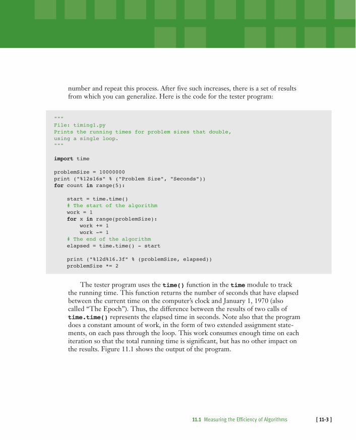
The output of this program is shown in Figure 11.4.

[FIGURE 11.4] The output of a tester program that runs the Fibonacci function

As the problem size doubles, the instruction count (number of recursive calls)grows slowly at first and then quite rapidly. At first, the instruction count is lessthan the square of the problem size, but the instruction count of 1973 is signifi-cantly larger than 256, the square of the problem size 16.

The problem with tracking counts in this way is that, with some algorithms,the computer still cannot run fast enough to show the counts for very large prob-lem sizes. Counting instructions is the right idea, but we need to turn to logicand mathematical reasoning for a complete method of analysis. The only tools weneed for this type of analysis are paper and pencil.

11.1.3 Measuring the Memory Used by an Algorithm

A complete analysis of the resources used by an algorithm includes the amount ofmemory required. Once again, we focus on rates of potential growth. Some algo-rithms require the same amount of memory to solve any problem. Other algo-rithms require more memory as the problem size gets larger.

Problem Size2481632

Calls1541

19734356617


11.1 Exercises

1 Write a tester program that counts and displays the number of iterationsof the following loop:

whileƒproblemSizeƒ>ƒ0:ƒƒƒƒproblemSizeƒ=ƒproblemSizeƒ//ƒ2

2 Run the program you created in Exercise 1 using problem sizes of 1000,2000, 4000, 10,000, and 100,000. As the problem size doubles orincreases by a factor of 10, what happens to the number of iterations?

3 The difference between the results of two calls of the time functiontime() is an elapsed time. Because the operating system might use theCPU for part of this time, the elapsed time might not reflect the actualtime that a Python code segment uses the CPU. Browse the Python doc-umentation for an alternative way of recording the processing time anddescribe how this would be done.

11.2 Complexity Analysis

In this section, we develop a method of determining the efficiency of algorithms thatallows us to rate them independently of platform-dependent timings or impracticalinstruction counts. This method, called complexity analysis, entails reading thealgorithm and using pencil and paper to work out some simple algebra.

11.2.1 Orders of Complexity

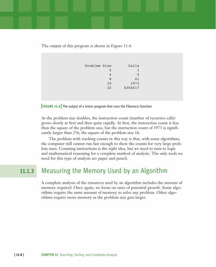
Consider the two counting loops discussed earlier. The first loop executes n timesfor a problem of size n. The second loop contains a nested loop that iterates n2

times. The amount of work done by these two algorithms is similar for small val-ues of n, but is very different for large values of n. Figure 11.5 and Table 11.1illustrate this divergence. Note that when we say “work,” we usually mean thenumber of iterations of the most deeply nested loop.

11.2 Complexity Analysis [ 11-9 ]

[FIGURE 11.5] A graph of the amounts of work done in the tester programs

[TABLE 11.1] The amounts of work in the tester programs

The performances of these algorithms differ by what we call an order ofcomplexity. The performance of the first algorithm is linear in that its workgrows in direct proportion to the size of the problem (problem size of 10, workof 10, 20 and 20, etc.). The behavior of the second algorithm is quadratic in thatits work grows as a function of the square of the problem size (problem size of10, work of 100). As you can see from the graph and the table, algorithms withlinear behavior do less work than algorithms with quadratic behavior for mostproblem sizes n. In fact, as the problem size gets larger, the performance of analgorithm with the higher order of complexity becomes worse more quickly.

Several other orders of complexity are commonly used in the analysis ofalgorithms. An algorithm has constant performance if it requires the same num-ber of operations for any problem size. List indexing is a good example of a con-stant-time algorithm. This is clearly the best kind of performance to have.

Another order of complexity that is better than linear but worse than con-stant is called logarithmic. The amount of work of a logarithmic algorithm isproportional to the log2 of the problem size. Thus, when the problem doubles insize, the amount of work only increases by 1 (that is, just add 1).

WORK OF THE FIRST WORK OF THE SECOND PROBLEM SIZE ALGORITHM ALGORITHM

2 2 4

10 10 100

1000 1000 1,000,000

Problem sizeO

pera

tions

n2 n


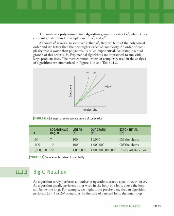
The work of a polynomial time algorithm grows at a rate of nk, where k is aconstant greater than 1. Examples are n2, n3, and n10.

Although n3 is worse in some sense than n2, they are both of the polynomialorder and are better than the next higher order of complexity. An order of com-plexity that is worse than polynomial is called exponential. An example rate ofgrowth of this order is 2n. Exponential algorithms are impractical to run withlarge problem sizes. The most common orders of complexity used in the analysisof algorithms are summarized in Figure 11.6 and Table 11.2.

[FIGURE 11.6] A graph of some sample orders of complexity

[TABLE 11.2] Some sample orders of complexity

11.2.2 Big-O Notation

An algorithm rarely performs a number of operations exactly equal to n, n2, or kn.An algorithm usually performs other work in the body of a loop, above the loop,and below the loop. For example, we might more precisely say that an algorithmperforms 2n + 3 or 2n2 operations. In the case of a nested loop, the inner loop

LOGARITHMIC LINEAR QUADRATIC EXPONENTIALn (log2n) (n) (n2) (2nn)

100 7 100 10,000 Off the charts

1000 10 1000 1,000,000 Off the charts

1,000,000 20 1,000,000 1,000,000,000,000 Really off the charts

Problem size

Ope

ratio

nsn2 n

log2n

2n

11.2 Complexity Analysis [ 11-11 ]

might execute one less pass after each pass through the outer loop, so that thetotal number of iterations might be more like 1⁄ 2 n2 – 1⁄ 2 n, rather than n2.

The amount of work in an algorithm typically is the sum of several terms in apolynomial. Whenever the amount of work is expressed as a polynomial, we focuson one term as dominant. As n becomes large, the dominant term becomes solarge that the amount of work represented by the other terms can be ignored.Thus, for example, in the polynomial 1⁄ 2 n2 – 1⁄ 2 n, we focus on the quadraticterm, 1⁄ 2 n2, in effect dropping the linear term, 1⁄ 2 n, from consideration. We canalso drop the coefficient 1⁄ 2 because the ratio between 1⁄ 2 n2 and n2 does notchange as n grows. For example, if you double the problem size, the run times ofalgorithms that are 1⁄ 2 n2 and n2 both increase by a factor of 4. This type of analy-sis is sometimes called asymptotic analysis because the value of a polynomialasymptotically approaches or approximates the value of its largest term as nbecomes very large.

One notation that computer scientists use to express the efficiency or compu-tational complexity of an algorithm is called big-O notation. “O” stands for “onthe order of,” a reference to the order of complexity of the work of the algo-rithm. Thus, for example, the order of complexity of a linear-time algorithm isO(n). Big-O notation formalizes our discussion of orders of complexity.

11.2.3 The Role of the Constant of Proportionality

The constant of proportionality involves the terms and coefficients that areusually ignored during big-O analysis. However, when these items are large, theymay have an impact on the algorithm, particularly for small and medium-sizeddata sets. For example, no one can ignore the difference between n and n / 2,when n is $1,000,000. In the example algorithms discussed thus far, the instruc-tions that execute within a loop are part of the constant of proportionality, as arethe instructions that initialize the variables before the loops are entered. Whenanalyzing an algorithm, one must be careful to determine that any instructions donot hide a loop that depends on a variable problem size. If that is the case, thenthe analysis must move down into the nested loop, as we saw in the last example.

Let’s determine the constant of proportionality for the first algorithm dis-cussed in this chapter. Here is the code:

workƒ=ƒ1forƒxƒinƒrange(problemSize):ƒƒƒƒworkƒ+=ƒ1ƒƒƒƒworkƒ-=ƒ1


Note that, aside from the loop itself, there are three lines of code, each of themassignment statements. Each of these three statements runs in constant time.Let’s also assume that on each iteration, the overhead of managing the loop,which is hidden in the loop header, runs an instruction that requires constanttime. Thus, the amount of abstract work performed by this algorithm is 3n + 1.Although this number is greater than just n, the running times for the twoamounts of work, n and 3n + 1, increase at the same rate.

11.2 Exercises

1 Assume that each of the following expressions indicates the number ofoperations performed by an algorithm for a problem size of n. Point outthe dominant term of each algorithm, and use big-O notation to classify it.

a 2n – 4n2 + 5nb 3n2 + 6c n3 + n2 – n

2 For problem size n, algorithms A and B perform n2 and 1⁄ 2 n2 + 1⁄ 2 ninstructions, respectively. Which algorithm does more work? Are thereparticular problem sizes for which one algorithm performs significantlybetter than the other? Are there particular problem sizes for which bothalgorithms perform approximately the same amount of work?

3 At what point does an n4 algorithm begin to perform better than a2n algorithm?

11.3 Search Algorithms

We now present several algorithms that can be used for searching and sortinglists. We first discuss the design of an algorithm, we then show its implementa-tion as a Python function, and, finally, we provide an analysis of the algorithm’scomputational complexity. To keep things simple, each function processes a list ofintegers. Lists of different sizes can be passed as parameters to the functions. Thefunctions are defined in a single module that is used in the case study later in thischapter.

11.3 Search Algorithms [ 11-13 ]

11.3.1 Search for a Minimum

Python’s min function returns the minimum or smallest item in a list. To studythe complexity of this algorithm, let’s develop an alternative version that returnsthe position of the minimum item. The algorithm assumes that the list is notempty and that the items are in arbitrary order. The algorithm begins by treatingthe first position as that of the minimum item. It then searches to the right for anitem that is smaller and, if it is found, resets the position of the minimum item tothe current position. When the algorithm reaches the end of the list, it returnsthe position of the minimum item. Here is the code for the algorithm, in func-tion ourMin:

defƒourMin(lyst):ƒƒƒƒ“””Returnsƒtheƒpositionƒofƒtheƒminimumƒitem.”””ƒƒƒƒminposƒ=ƒ0ƒƒƒƒcurrentƒ=ƒ1ƒƒƒƒwhileƒcurrentƒ<ƒlen(lyst):ƒƒƒƒƒƒƒƒifƒlyst[current]ƒ<ƒlyst[minpos]:ƒƒƒƒƒƒƒƒƒƒƒƒminposƒ=ƒcurrentƒƒƒƒƒƒƒƒcurrentƒ+=ƒ1ƒƒƒƒreturnƒminpos

As you can see, there are three instructions outside the loop that execute thesame number of times regardless of the size of the list. Thus, we can discountthem. Within the loop, we find three more instructions. Of these, the compari-son in the if statement and the increment of current execute on each passthrough the loop. There are no nested or hidden loops in these instructions. Thisalgorithm must visit every item in the list to guarantee that it has located theposition of the minimum item. Thus, the algorithm must make n – 1 comparisonsfor a list of size n. Therefore, the algorithm’s complexity is O(n).

11.3.2 Linear Search of a List

Python’s in operator is implemented as a method named __contains__ in thelist class. This method searches for a particular item (called the target item)within a list of arbitrarily arranged items. In such a list, the only way to search fora target item is to begin with the item at the first position and compare it to thetarget. If the items are equal, the method returns True. Otherwise, the methodmoves on to the next position and compares items again. If the method arrives atthe last position and still cannot find the target, it returns False. This kind of


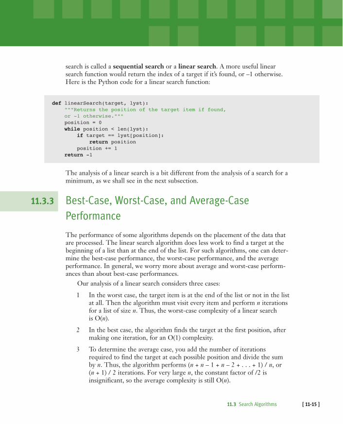
search is called a sequential search or a linear search. A more useful linearsearch function would return the index of a target if it’s found, or –1 otherwise.Here is the Python code for a linear search function:

defƒlinearSearch(target,ƒlyst):ƒƒƒƒ“””Returnsƒtheƒpositionƒofƒtheƒtargetƒitemƒifƒfound,ƒƒƒƒorƒ-1ƒotherwise.”””ƒƒƒƒpositionƒ=ƒ0ƒƒƒƒwhileƒpositionƒ<ƒlen(lyst):ƒƒƒƒƒƒƒƒifƒtargetƒ==ƒlyst[position]:ƒƒƒƒƒƒƒƒƒƒƒƒreturnƒpositionƒƒƒƒƒƒƒƒpositionƒ+=ƒ1ƒƒƒƒreturnƒ-1

The analysis of a linear search is a bit different from the analysis of a search for aminimum, as we shall see in the next subsection.

11.3.3 Best-Case, Worst-Case, and Average-Case

Performance

The performance of some algorithms depends on the placement of the data thatare processed. The linear search algorithm does less work to find a target at thebeginning of a list than at the end of the list. For such algorithms, one can deter-mine the best-case performance, the worst-case performance, and the averageperformance. In general, we worry more about average and worst-case perform-ances than about best-case performances.

Our analysis of a linear search considers three cases:

1 In the worst case, the target item is at the end of the list or not in the listat all. Then the algorithm must visit every item and perform n iterationsfor a list of size n. Thus, the worst-case complexity of a linear searchis O(n).

2 In the best case, the algorithm finds the target at the first position, aftermaking one iteration, for an O(1) complexity.

3 To determine the average case, you add the number of iterationsrequired to find the target at each possible position and divide the sumby n. Thus, the algorithm performs (n + n – 1 + n – 2 + . . . + 1) / n, or(n + 1) / 2 iterations. For very large n, the constant factor of /2 isinsignificant, so the average complexity is still O(n).


Clearly, the best-case performance of a linear search is rare when comparedwith the average and worst-case performances, which are essentially the same.

11.3.4 Binary Search of a List

A linear search is necessary for data that are not arranged in any particular order.When searching sorted data, you can use a binary search.

To understand how a binary search works, think about what happens whenyou look up a person’s number in a phone book. The data in a phone book arealready sorted, so you don’t do a linear search. Instead, you estimate the name’salphabetical position in the book, and open the book as close to that position aspossible. After you open the book, you determine if the target name lies, alpha-betically, on an earlier page or later page, and flip back or forward through thepages as necessary. You repeat this process until you find the name or concludethat it’s not in the book.

Now let’s consider an example of a binary search in Python. To begin, let’sassume that the items in the list are sorted in ascending order (as they are in aphone book). The search algorithm goes directly to the middle position in the listand compares the item at that position to the target. If there is a match, the algo-rithm returns the position. Otherwise, if the target is less than the current item,the algorithm searches the portion of the list before the middle position. If thetarget is greater than the current item, the algorithm searches the portion of thelist after the middle position. The search process stops when the target is foundor the current beginning position is greater than the current ending position.

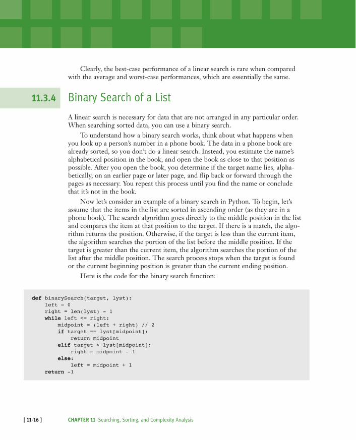
Here is the code for the binary search function:

defƒbinarySearch(target,ƒlyst):ƒƒƒƒleftƒ=ƒ0ƒƒƒƒrightƒ=ƒlen(lyst)ƒ-ƒ1ƒƒƒƒwhileƒleftƒ<=ƒright:ƒƒƒƒƒƒƒƒmidpointƒ=ƒ(leftƒ+ƒright)ƒ//ƒ2ƒƒƒƒƒƒƒƒifƒtargetƒ==ƒlyst[midpoint]:ƒƒƒƒƒƒƒƒƒƒƒƒreturnƒmidpointƒƒƒƒƒƒƒƒelifƒtargetƒ<ƒlyst[midpoint]:ƒƒƒƒƒƒƒƒƒƒƒƒrightƒ=ƒmidpointƒ-ƒ1ƒƒƒƒƒƒƒƒelse:ƒƒƒƒƒƒƒƒƒƒƒƒleftƒ=ƒmidpointƒ+ƒ1ƒƒƒƒreturnƒ-1


There is just one loop with no nested or hidden loops. Once again, the worst caseoccurs when the target is not in the list. How many times does the loop run inthe worst case? This is equal to the number of times the size of the list can bedivided by 2 until the quotient is 1. For a list of size n, you essentially performthe reduction n / 2 / 2 . . . / 2 until the result is 1. Let k be the number of timeswe divide n by 2. To solve for k, you have n / 2k = 1, and n = 2k, and k = log2n.Thus, the worst-case complexity of binary search is O(log2n).

Figure 11.7 shows the portions of the list being searched in a binary searchwith a list of 9 items and a target item, 10, that is not in the list. The items com-pared to the target are shaded. Note that none of the items in the left half of theoriginal list are visited.

[FIGURE 11.7] The items of a list visited during a binary search for 10

The binary search for the target item 10 requires four comparisons, whereasa linear search would have required 10 comparisons. This algorithm actuallyappears to perform better as the problem size gets larger. Our list of 9 itemsrequires at most 4 comparisons, whereas a list of 1,000,000 items requires at mostonly 20 comparisons!

Binary search is certainly more efficient than linear search. However, thekind of search algorithm we choose depends on the organization of the data inthe list. There is some additional overall cost to a binary search which has to dowith keeping the list in sorted order. In a moment, we examine several strategiesfor sorting a list and analyze their complexity. But first, we provide a few wordsabout comparing data items.

Comparison

1

2

3

4

1 2 3 4 5 6 7 8 9

1 2 3 4 6 7 8 9

1 3 4 7

4 9

8 9


11.3.5 Comparing Data Items

Both the binary search and the search for the minimum assume that the items inthe list are comparable with each other. In Python, this means that the items areof the same type and that they recognize the comparison operators ==, <, and >.Objects of several built-in Python types, such as numbers, strings, and lists, canbe compared using these operators.

To allow algorithms to use the comparison operators ==, <, and > with a newclass of objects, the programmer should define the __eq__, __lt__, and __gt__methods in that class. The header of __lt__ is the following:

defƒ__lt__(self,ƒother):

This method returns True if self is less than other, or False otherwise. Thecriteria for comparing the objects depend on their internal structure and on themanner in which they should be ordered.

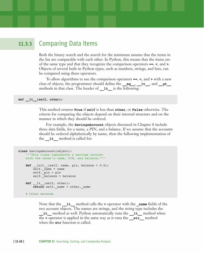
For example, the SavingsAccount objects discussed in Chapter 8 includethree data fields, for a name, a PIN, and a balance. If we assume that the accountsshould be ordered alphabetically by name, then the following implementation ofthe __lt__ method is called for:

classƒSavingsAccount(object):ƒƒƒƒ“””Thisƒclassƒrepresentsƒaƒsavingsƒaccountƒƒƒƒwithƒtheƒowner’sƒname,ƒPIN,ƒandƒbalance.”””

ƒƒƒƒdefƒ__init__(self,ƒname,ƒpin,ƒbalanceƒ=ƒ0.0):ƒƒƒƒƒƒƒƒself._nameƒ=ƒnameƒƒƒƒƒƒƒƒself._pinƒ=ƒpinƒƒƒƒƒƒƒƒself._balanceƒ=ƒbalance

ƒƒƒƒdefƒ__lt__(self,ƒother):ƒƒƒƒƒƒƒƒreturnƒself._nameƒ<ƒother._name

ƒƒƒƒ#ƒOtherƒmethods

Note that the __lt__ method calls the < operator with the _name fields of thetwo account objects. The names are strings, and the string type includes the__lt__ method as well. Python automatically runs the __lt__ method when the < operator is applied in the same way as it runs the __str__ methodwhen the str function is called.


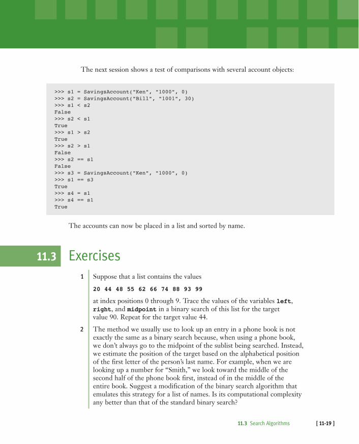
The next session shows a test of comparisons with several account objects:

>>>ƒs1ƒ=ƒSavingsAccount(“Ken”,ƒ“1000”,ƒ0)>>>ƒs2ƒ=ƒSavingsAccount(“Bill”,ƒ“1001”,ƒ30)>>>ƒs1ƒ<ƒs2False>>>ƒs2ƒ<ƒs1True>>>ƒs1ƒ>ƒs2True>>>ƒs2ƒ>ƒs1False>>>ƒs2ƒ==ƒs1False>>>ƒs3ƒ=ƒSavingsAccount(“Ken”,ƒ“1000”,ƒ0)>>>ƒs1ƒ==ƒs3True>>>ƒs4ƒ=ƒs1>>>ƒs4ƒ==ƒs1True

The accounts can now be placed in a list and sorted by name.

11.3 Exercises

1 Suppose that a list contains the values

20 44 48 55 62 66 74 88 93 99

at index positions 0 through 9. Trace the values of the variables left,right, and midpoint in a binary search of this list for the targetvalue 90. Repeat for the target value 44.

2 The method we usually use to look up an entry in a phone book is notexactly the same as a binary search because, when using a phone book,we don’t always go to the midpoint of the sublist being searched. Instead,we estimate the position of the target based on the alphabetical positionof the first letter of the person’s last name. For example, when we arelooking up a number for “Smith,” we look toward the middle of thesecond half of the phone book first, instead of in the middle of theentire book. Suggest a modification of the binary search algorithm thatemulates this strategy for a list of names. Is its computational complexityany better than that of the standard binary search?


11.4 Sort Algorithms

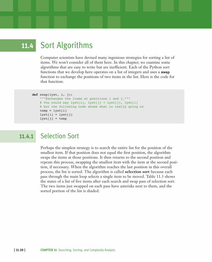
Computer scientists have devised many ingenious strategies for sorting a list ofitems. We won’t consider all of them here. In this chapter, we examine somealgorithms that are easy to write but are inefficient. Each of the Python sortfunctions that we develop here operates on a list of integers and uses a swapfunction to exchange the positions of two items in the list. Here is the code forthat function:

defƒswap(lyst,ƒi,ƒj):ƒƒƒƒ“””Exchangesƒtheƒitemsƒatƒpositionsƒiƒandƒj.”””ƒƒƒƒ#ƒYouƒcouldƒsayƒlyst[i],ƒlyst[j]ƒ=ƒlyst[j],ƒlyst[i]ƒƒƒƒ#ƒbutƒtheƒfollowingƒcodeƒshowsƒwhatƒisƒreallyƒgoingƒonƒƒƒƒtempƒ=ƒlyst[i]ƒƒƒƒlyst[i]ƒ=ƒlyst[j]ƒƒƒƒlyst[j]ƒ=ƒtemp

11.4.1 Selection Sort

Perhaps the simplest strategy is to search the entire list for the position of thesmallest item. If that position does not equal the first position, the algorithmswaps the items at those positions. It then returns to the second position andrepeats this process, swapping the smallest item with the item at the second posi-tion, if necessary. When the algorithm reaches the last position in this overallprocess, the list is sorted. The algorithm is called selection sort because eachpass through the main loop selects a single item to be moved. Table 11.3 showsthe states of a list of five items after each search and swap pass of selection sort.The two items just swapped on each pass have asterisks next to them, and thesorted portion of the list is shaded.


[TABLE 11.3] A trace of the data during a selection sort

Here is the Python function for a selection sort:

defƒselectionSort(lyst):ƒƒƒƒiƒ=ƒ0ƒƒƒƒwhileƒiƒ<ƒlen(lyst)ƒ-ƒ1:ƒƒƒƒƒƒƒƒƒ#ƒDoƒnƒ-ƒ1ƒsearchesƒƒƒƒƒƒƒƒminIndexƒ=ƒiƒƒƒƒƒƒƒƒƒƒƒƒƒƒƒƒƒ#ƒforƒtheƒsmallestƒƒƒƒƒƒƒƒjƒ=ƒiƒ+ƒ1ƒƒƒƒƒƒƒƒwhileƒjƒ<ƒlen(lyst):ƒƒƒƒƒƒƒƒƒ#ƒStartƒaƒsearchƒƒƒƒƒƒƒƒƒƒƒƒifƒlyst[j]ƒ<ƒlyst[minIndex]:ƒƒƒƒƒƒƒƒƒƒƒƒƒƒƒƒminIndexƒ=ƒjƒƒƒƒƒƒƒƒƒƒƒƒjƒ+=ƒ1ƒƒƒƒƒƒƒƒifƒminIndexƒ!=ƒi:ƒƒƒƒƒƒƒƒƒƒƒƒ#ƒExchangeƒifƒneededƒƒƒƒƒƒƒƒƒƒƒƒswap(lyst,ƒminIndex,ƒi)ƒƒƒƒƒƒƒƒiƒ+=ƒ1

This function includes a nested loop. For a list of size n, the outer loopexecutes n – 1 times. On the first pass through the outer loop, the inner loopexecutes n – 1 times. On the second pass through the outer loop, the inner loop exe-cutes n – 2 times. On the last pass through the outer loop, the inner loop executesonce. Thus, the total number of comparisons for a list of size n is the following:

(n – 1) + (n – 2) + … + 1 =n (n – 1) / 2 =1⁄ 2 n2 – 1⁄ 2 n

For large n, you can pick the term with the largest degree and drop the coeffi-cient, so selection sort is O(n2) in all cases. For large data sets, the cost of swappingitems might also be significant. Because data items are swapped only in the outerloop, this additional cost for selection sort is linear in the worst and average cases.

UNSORTED AFTER AFTER AFTER AFTER LIST 1st PASS 2nd PASS 3rd PASS 4th PASS

5 1* 1 1 1

3 3 2* 2 2

1 5* 5 3* 3

2 2 3* 5* 4*

4 4 4 4 5*

11.4 Sort Algorithms [ 11-21 ]

11.4.2 Bubble Sort

Another sort algorithm that is relatively easy to conceive and code is called abubble sort. Its strategy is to start at the beginning of the list and compare pairsof data items as it moves down to the end. Each time the items in the pair are outof order, the algorithm swaps them. This process has the effect of bubbling thelargest items to the end of the list. The algorithm then repeats the process fromthe beginning of the list and goes to the next-to-last item, and so on, until itbegins with the last item. At that point, the list is sorted.

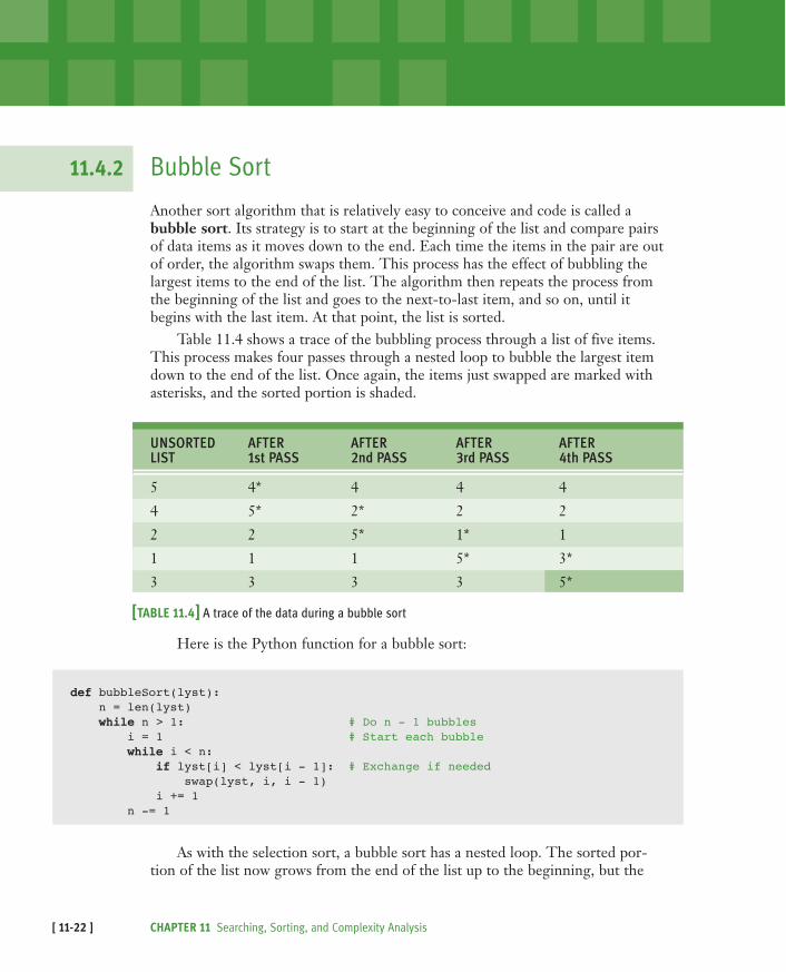
Table 11.4 shows a trace of the bubbling process through a list of five items.This process makes four passes through a nested loop to bubble the largest itemdown to the end of the list. Once again, the items just swapped are marked withasterisks, and the sorted portion is shaded.

[TABLE 11.4] A trace of the data during a bubble sort

Here is the Python function for a bubble sort:

defƒbubbleSort(lyst):ƒƒƒƒnƒ=ƒlen(lyst)ƒƒƒƒwhileƒnƒ>ƒ1:ƒƒƒƒƒƒƒƒƒƒƒƒƒƒƒƒƒƒƒƒƒƒƒ#ƒDoƒnƒ-ƒ1ƒbubblesƒƒƒƒƒƒƒƒiƒ=ƒ1ƒƒƒƒƒƒƒƒƒƒƒƒƒƒƒƒƒƒƒƒƒƒƒƒƒƒ#ƒStartƒeachƒbubbleƒƒƒƒƒƒƒƒwhileƒiƒ<ƒn:ƒƒƒƒƒƒƒƒƒƒƒƒifƒlyst[i]ƒ<ƒlyst[iƒ-ƒ1]:ƒƒ#ƒExchangeƒifƒneededƒƒƒƒƒƒƒƒƒƒƒƒƒƒƒƒswap(lyst,ƒi,ƒiƒ-ƒ1)ƒƒƒƒƒƒƒƒƒƒƒƒiƒ+=ƒ1ƒƒƒƒƒƒƒƒnƒ-=ƒ1

As with the selection sort, a bubble sort has a nested loop. The sorted por-tion of the list now grows from the end of the list up to the beginning, but the


5 4* 4 4 4

4 5* 2* 2 2

2 2 5* 1* 1

1 1 1 5* 3*

3 3 3 3 5*


performance of the bubble sort is quite similar to the behavior of selection sort:the inner loop executes 1⁄ 2 n2 – 1⁄ 2 n times for a list of size n. Thus, bubble sort isO(n2). Like selection sort, bubble sort won’t perform any swaps if the list isalready sorted. However, bubble sort’s worst-case behavior for exchanges isgreater than linear. The proof of this is left as an exercise for you.

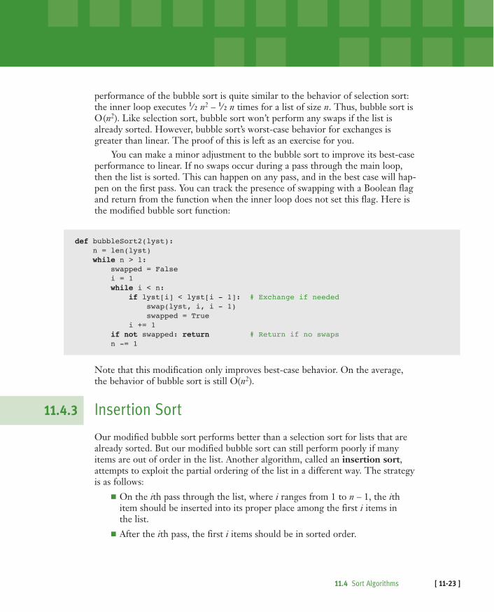
You can make a minor adjustment to the bubble sort to improve its best-caseperformance to linear. If no swaps occur during a pass through the main loop,then the list is sorted. This can happen on any pass, and in the best case will hap-pen on the first pass. You can track the presence of swapping with a Boolean flagand return from the function when the inner loop does not set this flag. Here isthe modified bubble sort function:

defƒbubbleSort2(lyst):ƒƒƒƒnƒ=ƒlen(lyst)ƒƒƒƒwhileƒnƒ>ƒ1:ƒƒƒƒƒƒƒƒswappedƒ=ƒFalseƒƒƒƒƒƒƒƒiƒ=ƒ1ƒƒƒƒƒƒƒƒwhileƒiƒ<ƒn:ƒƒƒƒƒƒƒƒƒƒƒƒifƒlyst[i]ƒ<ƒlyst[iƒ-ƒ1]:ƒƒ#ƒExchangeƒifƒneededƒƒƒƒƒƒƒƒƒƒƒƒƒƒƒƒswap(lyst,ƒi,ƒiƒ-ƒ1)ƒƒƒƒƒƒƒƒƒƒƒƒƒƒƒƒswappedƒ=ƒTrueƒƒƒƒƒƒƒƒƒƒƒƒiƒ+=ƒ1ƒƒƒƒƒƒƒƒifƒnotƒswapped:ƒreturnƒƒƒƒƒƒƒƒƒ#ƒReturnƒifƒnoƒswapsƒƒƒƒƒƒƒƒnƒ-=ƒ1

Note that this modification only improves best-case behavior. On the average,the behavior of bubble sort is still O(n2).

11.4.3 Insertion Sort

Our modified bubble sort performs better than a selection sort for lists that arealready sorted. But our modified bubble sort can still perform poorly if manyitems are out of order in the list. Another algorithm, called an insertion sort,attempts to exploit the partial ordering of the list in a different way. The strategyis as follows:

� On the ith pass through the list, where i ranges from 1 to n – 1, the ithitem should be inserted into its proper place among the first i items inthe list.

� After the ith pass, the first i items should be in sorted order.


� This process is analogous to the way in which many people organize play-ing cards in their hands. That is, if you hold the first i – 1 cards in order,you pick the ith card and compare it to these cards until its proper spotis found.

� As with our other sort algorithms, insertion sort consists of two loops. Theouter loop traverses the positions from 1 to n – 1. For each position i inthis loop, you save the item and start the inner loop at position i – 1. Foreach position j in this loop, you move the item to position j + 1 until youfind the insertion point for the saved (ith) item.

Here is the code for the insertionSort function:

defƒinsertionSort(lyst):ƒƒƒƒiƒ=ƒ1ƒƒƒƒwhileƒiƒ<ƒlen(lyst):ƒƒƒƒƒƒƒƒitemToInsertƒ=ƒlyst[i]ƒƒƒƒƒƒƒƒjƒ=ƒiƒ-ƒ1ƒƒƒƒƒƒƒƒwhileƒjƒ>=ƒ0:ƒƒƒƒƒƒƒƒƒƒƒƒifƒitemToInsertƒ<ƒlyst[j]:ƒƒƒƒƒƒƒƒƒƒƒƒƒƒƒƒlyst[jƒ+ƒ1]ƒ=ƒlyst[j]ƒƒƒƒƒƒƒƒƒƒƒƒƒƒƒƒjƒ-=ƒ1ƒƒƒƒƒƒƒƒƒƒƒƒelse:ƒƒƒƒƒƒƒƒƒƒƒƒƒƒƒƒbreakƒƒƒƒƒƒƒƒlyst[jƒ+ƒ1]ƒ=ƒitemToInsertƒƒƒƒƒƒƒƒiƒ+=ƒ1

Table 11.5 shows the states of a list of five items after each pass through theouter loop of an insertion sort. The item to be inserted on the next pass ismarked with an arrow; after it is inserted, this item is marked with an asterisk.

[TABLE 11.5] A trace of the data during an insertion sort


2 2 1* 1 1

5 ← 5 (no insertion) 2 2 2

1 1← 5 4* 3*

4 4 4 ← 5 4

3 3 3 3 ← 5


Once again, analysis focuses on the nested loop. The outer loop executes n – 1times. In the worst case, when all of the data are out of order, the inner loop iter-ates once on the first pass through the outer loop, twice on the second pass, andso on, for a total of 1⁄ 2 n2 – 1⁄ 2 n times. Thus, the worst-case behavior of insertionsort is O(n2).

The more items in the list that are in order, the better insertion sort getsuntil, in the best case of a sorted list, the sort’s behavior is linear. In the averagecase, however, insertion sort is still quadratic.

11.4.4 Best-Case, Worst-Case, and Average-Case

Performance Revisited

As mentioned earlier, for many algorithms, a single measure of complexity cannotbe applied to all cases. Sometimes an algorithm’s behavior improves or gets worsewhen it encounters a particular arrangement of data. For example, the bubblesort algorithm can terminate as soon as the list becomes sorted. If the input listis already sorted, the bubble sort requires approximately n comparisons. In manyother cases, however, bubble sort requires approximately n2 comparisons. Clearly,a more detailed analysis may be needed to make programmers aware of thesespecial cases.

As we discussed earlier, thorough analysis of an algorithm’s complexitydivides its behavior into three types of cases:

1 Best case—Under what circumstances does an algorithm do the leastamount of work? What is the algorithm’s complexity in this best case?

2 Worst case—Under what circumstances does an algorithm do the mostamount of work? What is the algorithm’s complexity in this worst case?

3 Average case—Under what circumstances does an algorithm do a typicalamount of work? What is the algorithm’s complexity in this typical case?

Let’s review three examples of this kind of analysis for a search for a minimum,linear search, and bubble sort.

Because the search for a minimum algorithm must visit each number in thelist, unless it is sorted, the algorithm is always linear. Therefore, its best-case,worst-case, and average-case performances are O(n).


Linear search is a bit different. The algorithm stops and returns a result assoon as it finds the target item. Clearly, in the best case, the target element is in thefirst position. In the worst case, the target is in the last position. Therefore, thealgorithm’s best-case performance is O(1), and its worst-case performance is O(n).To compute the average-case performance, we add up all of the comparisonsthat must be made to locate a target in each position and divide by n. This is(1 + 2 + . . . + n) / n, or n / 2. Therefore, by approximation, the average-caseperformance of linear search is also O(n).

The smarter version of bubble sort can terminate as soon as the list becomessorted. In the best case, this happens when the input list is already sorted.Therefore, bubble sort’s best-case performance is O(n). However, this case is rare(1 out of n!). In the worst case, even this version of bubble sort will have to bub-ble each item down to its proper position in the list. The algorithm’s worst-caseperformance is clearly O(n2). Bubble sort’s average-case performance is closer toO(n2) than to O(n), although the demonstration of this fact is a bit more involvedthan it is for linear search.

As we will see, there are algorithms whose best-case and average-caseperformances are similar, but whose performance can degrade to a worst case.Whether you are choosing an algorithm or developing a new one, it is importantto be aware of these distinctions.

11.4 Exercises

1 Which configuration of data in a list causes the smallest number ofexchanges in a selection sort? Which configuration of data causes thelargest number of exchanges?

2 Explain the role that the number of data exchanges plays in the analysisof selection sort and bubble sort. What role, if any, does the size of thedata objects play?

3 Explain why the modified bubble sort still exhibits O(n2) behavior onthe average.

4 Explain why insertion sort works well on partially sorted lists.


11.5 An Exponential Algorithm: RecursiveFibonacci

Earlier in this chapter, we ran the recursive Fibonacci function to obtain a countof the recursive calls with various problem sizes. You saw that the number of callsseemed to grow much faster than the square of the problem size. Here is thecode for the function once again:

defƒfib(n):ƒƒƒƒ“””TheƒrecursiveƒFibonacciƒfunction.”””ƒƒƒƒifƒnƒ<ƒ3:ƒƒƒƒƒƒƒƒreturnƒ1ƒƒƒƒelse:ƒƒƒƒƒƒƒƒreturnƒfib(nƒ-ƒ1)ƒ+ƒfib(nƒ-ƒ2)

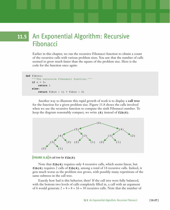
Another way to illustrate this rapid growth of work is to display a call treefor the function for a given problem size. Figure 11.8 shows the calls involvedwhen we use the recursive function to compute the sixth Fibonacci number. Tokeep the diagram reasonably compact, we write (6) instead of fib(6).

[FIGURE 11.8] A call tree for fib(6)

Note that fib(4) requires only 4 recursive calls, which seems linear, butfib(6) requires 2 calls of fib(4), among a total of 14 recursive calls. Indeed, itgets much worse as the problem size grows, with possibly many repetitions of thesame subtrees in the call tree.

Exactly how bad is this behavior, then? If the call tree were fully balanced,with the bottom two levels of calls completely filled in, a call with an argumentof 6 would generate 2 + 4 + 8 + 16 = 30 recursive calls. Note that the number of

(6)

(5)

(4) (3)

(4)

(3) (2)

(3)

(2) (1)

(2) (1)(2) (2) (1)

11.5 An Exponential Algorithm: Recursive Fibonacci [ 11-27 ]

calls at each filled level is twice that of the level above it. Thus, the number ofrecursive calls generally is 2n+1 – 2 in fully balanced call trees, where n is theargument at the top or root of the call tree. This is clearly the behavior of anexponential, O(kn) algorithm. Although the bottom two levels of the call tree forrecursive Fibonacci are not completely filled in, its call tree is close enough inshape to a fully balanced tree to rank recursive Fibonacci as an exponential algo-rithm. The constant k for recursive Fibonacci is approximately 1.63.

Exponential algorithms are generally impractical to run with any but verysmall problem sizes. Although recursive Fibonacci is elegant in its design, there isa less beautiful but much faster version that uses a loop to run in linear time (seethe next section).

Alternatively, recursive functions that are called repeatedly with the samearguments, such as the Fibonacci function, can be made more efficient by a tech-nique called memoization. According to this technique, the program maintains atable of the values for each argument used with the function. Before the functionrecursively computes a value for a given argument, it checks the table to see if thatargument already has a value. If so, that value is simply returned. If not, the com-putation proceeds, and the argument and value are added to the table afterward.

Computer scientists devote much effort to the development of fast algo-rithms. As a rule, any reduction in the order of magnitude of complexity, say,from O(n2) to O(n), is preferable to a “tweak” of code that reduces the constantof proportionality.

11.6 Converting Fibonacci to a Linear Algorithm

Although the recursive Fibonacci function reflects the simplicity and elegance ofthe recursive definition of the Fibonacci sequence, the run-time performance ofthis function is unacceptable. A different algorithm improves on this performanceby several orders of magnitude and, in fact, reduces the complexity to linear time.In this section, we develop this alternative algorithm and assess its performance.

Recall that the first two numbers in the Fibonacci sequence are 1s, and eachnumber after that is the sum of the previous two numbers. Thus, the new algo-rithm starts a loop if n is at least the third Fibonacci number. This number will beat least the sum of the first two (1 + 1 = 2). The loop computes this sum and thenperforms two replacements: the first number becomes the second one, and thesecond one becomes the sum just computed. The loop counts from 3 through n.


The sum at the end of the loop is the nth Fibonacci number. Here is thepseudocode for this algorithm:

Set sum to 1Set first to 1Set second to 1Set count to 3While count <= NƒƒƒƒSet sum to first + secondƒƒƒƒSet first to secondƒƒƒƒSet second to sumƒƒƒƒIncrement count

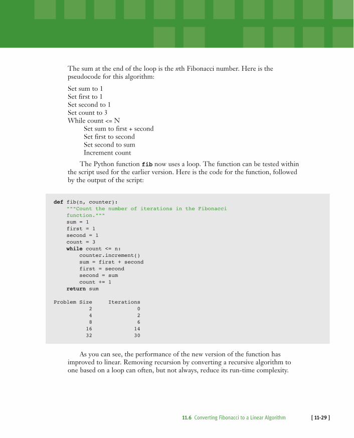
The Python function fib now uses a loop. The function can be tested withinthe script used for the earlier version. Here is the code for the function, followedby the output of the script:

defƒfib(n,ƒcounter):ƒƒƒƒ“””CountƒtheƒnumberƒofƒiterationsƒinƒtheƒFibonacciƒƒƒƒfunction.”””ƒƒƒƒsumƒ=ƒ1ƒƒƒƒfirstƒ=ƒ1ƒƒƒƒsecondƒ=ƒ1ƒƒƒƒcountƒ=ƒ3ƒƒƒƒwhileƒcountƒ<=ƒn:ƒƒƒƒƒƒƒƒcounter.increment()ƒƒƒƒƒƒƒƒsumƒ=ƒfirstƒ+ƒsecondƒƒƒƒƒƒƒƒfirstƒ=ƒsecondƒƒƒƒƒƒƒƒsecondƒ=ƒsumƒƒƒƒƒƒƒƒcountƒ+=ƒ1ƒƒƒƒreturnƒsum

ProblemƒSizeƒƒƒƒƒIterationsƒƒƒƒƒƒƒƒƒƒƒ2ƒƒƒƒƒƒƒƒƒƒƒƒƒƒ0ƒƒƒƒƒƒƒƒƒƒƒ4ƒƒƒƒƒƒƒƒƒƒƒƒƒƒ2ƒƒƒƒƒƒƒƒƒƒƒ8ƒƒƒƒƒƒƒƒƒƒƒƒƒƒ6ƒƒƒƒƒƒƒƒƒƒ16ƒƒƒƒƒƒƒƒƒƒƒƒƒ14ƒƒƒƒƒƒƒƒƒƒ32ƒƒƒƒƒƒƒƒƒƒƒƒƒ30

As you can see, the performance of the new version of the function hasimproved to linear. Removing recursion by converting a recursive algorithm toone based on a loop can often, but not always, reduce its run-time complexity.

11.6 Converting Fibonacci to a Linear Algorithm [ 11-29 ]


11.7 Case Study: An Algorithm Profiler

Profiling is the process of measuring an algorithm’s performance, by countinginstructions and/or timing execution. In this case study, we develop a program toprofile sort algorithms.

11.7.1 Request

Write a program that allows a programmer to profile different sort algorithms.

11.7.2 Analysis

The profiler should allow a programmer to run a sort algorithm on a list of num-bers. The profiler can track the algorithm’s running time, the number of compar-isons, and the number of exchanges. In addition, when the algorithm exchangestwo values, the profiler can print a trace of the list. The programmer can provideher own list of numbers to the profiler or ask the profiler to generate a list ofrandomly ordered numbers of a given size. The programmer can also ask for alist of unique numbers or a list that contains duplicate values. For ease of use, theprofiler allows the programmer to specify most of these features as options beforethe algorithm is run. The default behavior is to run the algorithm on a randomlyordered list of 10 unique numbers where the running time, comparisons, andexchanges are tracked.

The profiler is an instance of the class Profiler. The programmer profiles asort function by running the profiler’s test method with the function as the firstargument and any of the options mentioned earlier. The next session shows severaltest runs of the profiler with the selection sort algorithm and different options:

>>>ƒfromƒprofilerƒimportƒProfiler>>>ƒfromƒalgorithmsƒimportƒselectionSort

>>>ƒpƒ=ƒProfiler()

>>>ƒp.test(selectionSort)ƒƒƒƒƒ#ƒDefaultƒbehaviorProblemƒsize:ƒ10Elapsedƒtime:ƒ0.0Comparisons:ƒƒ45Exchanges:ƒƒƒƒ7

continued

11.7 Case Study: An Algorithm Profiler [ 11-31 ]

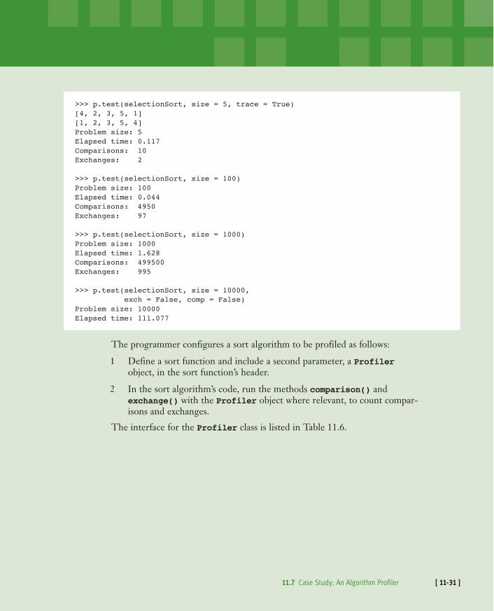
>>>ƒp.test(selectionSort,ƒsizeƒ=ƒ5,ƒtraceƒ=ƒTrue)[4,ƒ2,ƒ3,ƒ5,ƒ1][1,ƒ2,ƒ3,ƒ5,ƒ4]Problemƒsize:ƒ5Elapsedƒtime:ƒ0.117Comparisons:ƒƒ10Exchanges:ƒƒƒƒ2

>>>ƒp.test(selectionSort,ƒsizeƒ=ƒ100)Problemƒsize:ƒ100Elapsedƒtime:ƒ0.044Comparisons:ƒƒ4950Exchanges:ƒƒƒƒ97

>>>ƒp.test(selectionSort,ƒsizeƒ=ƒ1000)Problemƒsize:ƒ1000Elapsedƒtime:ƒ1.628Comparisons:ƒƒ499500Exchanges:ƒƒƒƒ995

>>>ƒp.test(selectionSort,ƒsizeƒ=ƒ10000,ƒƒƒƒƒƒƒƒƒƒƒƒexchƒ=ƒFalse,ƒcompƒ=ƒFalse)Problemƒsize:ƒ10000Elapsedƒtime:ƒ111.077

The programmer configures a sort algorithm to be profiled as follows:

1 Define a sort function and include a second parameter, a Profilerobject, in the sort function’s header.

2 In the sort algorithm’s code, run the methods comparison() andexchange() with the Profiler object where relevant, to count compar-isons and exchanges.

The interface for the Profiler class is listed in Table 11.6.


[TABLE 11.6] The interface for the Profiler class

11.7.3 Design

The programmer uses two modules:

1 profiler—This module defines the Profiler class.

2 algorithms—This module defines the sort functions, as configured forprofiling.

The sort functions have the same design as those discussed earlier in thischapter, except that they receive a Profiler object as an additional parameter.The Profiler methods comparison and exchange are run with this objectwhenever a sort function performs a comparison or an exchange of data values,respectively. In fact, any list-processing algorithm can be added to this moduleand profiled just by including a Profiler parameter and running its two meth-ods when comparisons and/or exchanges are made.

As shown in the earlier session, one imports the Profiler class and thealgorithms module into a Python shell and performs the testing at the shellprompt. The profiler’s test method sets up the Profiler object, runs the func-tion to be profiled, and prints the results.

Profiler METHOD WHAT IT DOES

p.test(function,ƒlystƒ=ƒNone,ƒ Runs function with the given ƒƒƒƒƒƒƒsizeƒ=ƒ10,ƒuniqueƒ=ƒTrue,ƒ settings and prints the results.ƒƒƒƒƒƒƒcompƒ=ƒTrue,ƒexchƒ=ƒTrue,ƒƒƒƒƒƒƒtraceƒ=ƒFalse)

p.comparison() Increments the number ofcomparisons if that option has beenspecified.

p.exchange() Increments the number of exchangesif that option has been specified.

p.__str__() Returns a string representation of theresults, depending on the options.


11.7.4 Implementation (Coding)

Here is a partial implementation of the algorithms module. We omit most ofthe sort algorithms developed earlier in this chapter, but include one,selectionSort, to show how the statistics are updated.

“””File:ƒalgorithms.pyAlgorithmsƒconfiguredƒforƒprofiling.“””

defƒselectionSort(lyst,ƒprofiler):ƒƒƒƒiƒ=ƒ0ƒƒƒƒwhileƒiƒ<ƒlen(lyst)ƒ-ƒ1:ƒƒƒƒƒƒƒƒƒƒƒƒƒƒƒƒƒminIndexƒ=ƒiƒƒƒƒƒƒƒƒjƒ=ƒiƒ+ƒ1ƒƒƒƒƒƒƒƒwhileƒjƒ<ƒlen(lyst):ƒƒƒƒƒƒƒƒƒƒƒƒprofiler.comparison()ƒƒƒƒƒƒƒƒƒ#ƒCountƒƒƒƒƒƒƒƒƒƒƒƒifƒlyst[j]ƒ<ƒlyst[minIndex]:ƒƒƒƒƒƒƒƒƒƒƒƒƒƒƒƒminIndexƒ=ƒjƒƒƒƒƒƒƒƒƒƒƒƒjƒ+=ƒ1ƒƒƒƒƒƒƒƒifƒminIndexƒ!=ƒi:ƒƒƒƒƒƒƒƒƒƒƒƒswap(lyst,ƒminIndex,ƒi,ƒprofiler)ƒƒƒƒƒƒƒƒiƒ+=ƒ1

defƒswap(lyst,ƒi,ƒj,ƒprofiler):ƒƒƒƒ“””Exchangesƒtheƒelementsƒatƒpositionsƒiƒandƒj.”””ƒƒƒƒprofiler.exchange()ƒƒƒƒƒƒƒƒƒƒƒƒƒƒƒƒƒƒƒ#ƒCountƒƒƒƒtempƒ=ƒlyst[i]ƒƒƒƒlyst[i]ƒ=ƒlyst[j]ƒƒƒƒlyst[j]ƒ=ƒtemp

#ƒTestingƒcodeƒcanƒgoƒhere,ƒoptionally

The Profiler class includes the four methods listed in the interface as wellas some helper methods for managing the clock.


“””File:ƒprofiler.py

Definesƒaƒclassƒforƒprofilingƒsortƒalgorithms.AƒProfilerƒobjectƒtracksƒtheƒlist,ƒtheƒnumberƒofƒcomparisonsandƒexchanges,ƒandƒtheƒrunningƒtime.ƒTheƒProfilerƒcanƒalsoprintƒaƒtraceƒandƒcanƒcreateƒaƒlistƒofƒuniqueƒorƒduplicatenumbers.

Exampleƒuse:

fromƒprofilerƒimportƒProfilerfromƒalgorithmsƒimportƒselectionSort

pƒ=ƒProfiler()p.test(selectionSort,ƒsizeƒ=ƒ15,ƒcompƒ=ƒTrue,ƒƒƒƒƒƒƒexchƒ=ƒTrue,ƒtraceƒ=ƒTrue)“””

importƒtimeimportƒrandom

classƒProfiler(object):

ƒƒƒƒdefƒtest(self,ƒfunction,ƒlystƒ=ƒNone,ƒsizeƒ=ƒ10,ƒƒƒƒƒƒƒƒƒƒƒƒƒuniqueƒ=ƒTrue,ƒcompƒ=ƒTrue,ƒexchƒ=ƒTrue,ƒƒƒƒƒƒƒƒƒƒƒƒƒtraceƒ=ƒFalse):ƒƒƒƒƒƒƒƒ“””ƒƒƒƒƒƒƒƒfunction:ƒtheƒalgorithmƒbeingƒprofiledƒƒƒƒƒƒƒƒtarget:ƒtheƒsearchƒtargetƒifƒprofilingƒaƒsearchƒƒƒƒƒƒƒƒlyst:ƒallowsƒtheƒcallerƒtoƒuseƒherƒlistƒƒƒƒƒƒƒƒsize:ƒtheƒsizeƒofƒtheƒlist,ƒ10ƒbyƒdefaultƒƒƒƒƒƒƒƒunique:ƒifƒTrue,ƒlistƒcontainsƒuniqueƒintegersƒƒƒƒƒƒƒƒcomp:ƒifƒTrue,ƒcountƒcomparisonsƒƒƒƒƒƒƒƒexch:ƒifƒTrue,ƒcountƒexchangesƒƒƒƒƒƒƒƒtrace:ƒifƒTrue,ƒprintƒtheƒlistƒafterƒeachƒexchangeƒƒƒƒƒƒƒƒƒƒƒƒƒƒƒƒRunƒtheƒfunctionƒwithƒtheƒgivenƒattributesƒandƒprintƒƒƒƒƒƒƒƒitsƒprofileƒresults.ƒƒƒƒƒƒƒƒ“””ƒƒƒƒƒƒƒƒself._compƒ=ƒcompƒƒƒƒƒƒƒƒself._exchƒ=ƒexchƒƒƒƒƒƒƒƒself._traceƒ=ƒtraceƒƒƒƒƒƒƒƒifƒlystƒ!=ƒNone:ƒƒƒƒƒƒƒƒƒƒƒƒself._lystƒ=ƒlystƒƒƒƒƒƒƒƒelifƒunique:ƒƒƒƒƒƒƒƒƒƒƒƒself._lystƒ=ƒlist(range(1,ƒsizeƒ+ƒ1))ƒƒƒƒƒƒƒƒƒƒƒƒrandom.shuffle(self._lyst)

continued


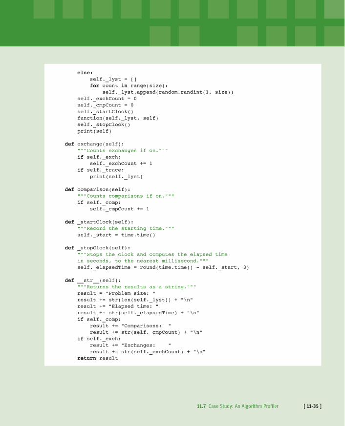
ƒƒƒƒƒƒƒƒelse:ƒƒƒƒƒƒƒƒƒƒƒƒself._lystƒ=ƒ[]ƒƒƒƒƒƒƒƒƒƒƒƒforƒcountƒinƒrange(size):ƒƒƒƒƒƒƒƒƒƒƒƒƒƒƒƒself._lyst.append(random.randint(1,ƒsize))ƒƒƒƒƒƒƒƒself._exchCountƒ=ƒ0ƒƒƒƒƒƒƒƒself._cmpCountƒ=ƒ0ƒƒƒƒƒƒƒƒself._startClock()ƒƒƒƒƒƒƒƒfunction(self._lyst,ƒself)ƒƒƒƒƒƒƒƒself._stopClock()ƒƒƒƒƒƒƒƒprint(self)

ƒƒƒƒdefƒexchange(self):ƒƒƒƒƒƒƒƒ“””Countsƒexchangesƒifƒon.”””ƒƒƒƒƒƒƒƒifƒself._exch:ƒƒƒƒƒƒƒƒƒƒƒƒself._exchCountƒ+=ƒ1ƒƒƒƒƒƒƒƒifƒself._trace:ƒƒƒƒƒƒƒƒƒƒƒƒprint(self._lyst)

ƒƒƒƒdefƒcomparison(self):ƒƒƒƒƒƒƒƒ“””Countsƒcomparisonsƒifƒon.”””ƒƒƒƒƒƒƒƒifƒself._comp:ƒƒƒƒƒƒƒƒƒƒƒƒself._cmpCountƒ+=ƒ1

ƒƒƒƒdefƒ_startClock(self):ƒƒƒƒƒƒƒƒ“””Recordƒtheƒstartingƒtime.”””ƒƒƒƒƒƒƒƒself._startƒ=ƒtime.time()

ƒƒƒƒdefƒ_stopClock(self):ƒƒƒƒƒƒƒƒ“””Stopsƒtheƒclockƒandƒcomputesƒtheƒelapsedƒtimeƒƒƒƒƒƒƒƒinƒseconds,ƒtoƒtheƒnearestƒmillisecond.”””ƒƒƒƒƒƒƒƒself._elapsedTimeƒ=ƒround(time.time()ƒ-ƒself._start,ƒ3)

ƒƒƒƒdefƒ__str__(self):ƒƒƒƒƒƒƒƒ“””Returnsƒtheƒresultsƒasƒaƒstring.”””ƒƒƒƒƒƒƒƒresultƒ=ƒ“Problemƒsize:ƒ“ƒƒƒƒƒƒƒƒresultƒ+=ƒstr(len(self._lyst))ƒ+ƒ“\n”ƒƒƒƒƒƒƒƒresultƒ+=ƒ“Elapsedƒtime:ƒ“ƒƒƒƒƒƒƒƒresultƒ+=ƒstr(self._elapsedTime)ƒ+ƒ“\n”ƒƒƒƒƒƒƒƒifƒself._comp:ƒƒƒƒƒƒƒƒƒƒƒƒresultƒ+=ƒ“Comparisons:ƒƒ“ƒƒƒƒƒƒƒƒƒƒƒƒƒresultƒ+=ƒstr(self._cmpCount)ƒ+ƒ“\n”ƒƒƒƒƒƒƒƒifƒself._exch:ƒƒƒƒƒƒƒƒƒƒƒƒresultƒ+=ƒ“Exchanges:ƒƒƒƒ“ƒƒƒƒƒƒƒƒƒƒƒƒƒresultƒ+=ƒstr(self._exchCount)ƒ+ƒ“\n”ƒƒƒƒƒƒƒƒreturnƒresult

Summary� Different algorithms for solving the same problem can be ranked

according to the time and memory resources that they require.Generally, algorithms that require less running time and less memoryare considered better than those that require more of these resources.However, there is often a tradeoff between the two types of resources.Running time can occasionally be improved at the cost of using morememory, or memory usage can be improved at the cost of slowerrunning times.

� The running time of an algorithm can be measured empiricallyusing the computer’s clock. However, these times will vary with thehardware and the types of programming language used.

� Counting instructions provides another empirical measurement of theamount of work that an algorithm does. Instruction counts can showincreases or decreases in the rate of growth of an algorithm’s work,independently of hardware and software platforms.

� The rate of growth of an algorithm’s work can be expressed as a func-tion of the size of its problem instances. Complexity analysis examinesthe algorithm’s code to derive these expressions. Such an expressionenables the programmer to predict how well or poorly an algorithmwill perform on any computer.

� Big-O notation is a common way of expressing an algorithm’s run-time behavior. This notation uses the form O(f(n)), where n is the sizeof the algorithm’s problem and f(n) is a function expressing theamount of work done to solve it.

� Common expressions of run-time behavior are O(log2n) (logarithmic),O(n) (linear), O(n2) (quadratic), and O(kn) (exponential).

� An algorithm can have different best-case, worst-case, and average-case behaviors. For example, bubble sort and insertion sort are linearin the best case, but quadratic in the average and worst cases.

� In general, it is better to try to reduce the order of an algorithm’scomplexity than it is to try to enhance performance by tweakingthe code.

� A binary search is substantially faster than a linear search. However,the data in the search space for a binary search must be in sorted order.

� Exponential algorithms are primarily of theoretical interest and areimpractical to run with large problem sizes.


REVIEW QUESTIONS [ 11-37 ]

REVIEW QUESTIONS

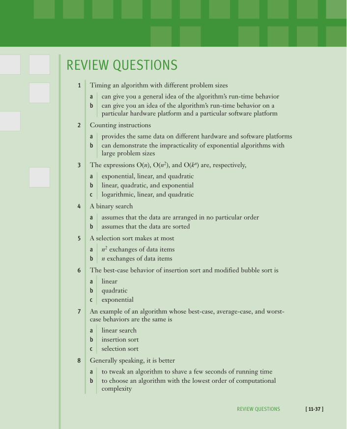
1 Timing an algorithm with different problem sizes

a can give you a general idea of the algorithm’s run-time behaviorb can give you an idea of the algorithm’s run-time behavior on a

particular hardware platform and a particular software platform

2 Counting instructions

a provides the same data on different hardware and software platformsb can demonstrate the impracticality of exponential algorithms with

large problem sizes

3 The expressions O(n), O(n2), and O(kn) are, respectively,

a exponential, linear, and quadraticb linear, quadratic, and exponentialc logarithmic, linear, and quadratic

4 A binary search

a assumes that the data are arranged in no particular orderb assumes that the data are sorted

5 A selection sort makes at most

a n2 exchanges of data itemsb n exchanges of data items

6 The best-case behavior of insertion sort and modified bubble sort is

a linearb quadraticc exponential

7 An example of an algorithm whose best-case, average-case, and worst-case behaviors are the same is

a linear searchb insertion sortc selection sort

8 Generally speaking, it is better

a to tweak an algorithm to shave a few seconds of running timeb to choose an algorithm with the lowest order of computational

complexity


9 The recursive Fibonacci function makes approximately

a n2 recursive calls for problems of a large size nb 2n recursive calls for problems of a large size n

10 Each level in a completely filled binary call tree has

a twice as many calls as the level above itb the same number of calls as the level above it

PROJECTS

1 A linear search of a sorted list can halt when the target is less than agiven element in the list. Define a modified version of this algorithm,and state the computational complexity, using big-O notation, of its best-, worst-, and average-case performances.

2 The list method reverse reverses the elements in the list. Define afunction named reverse that reverses the elements in its list argument(without using the method reverse!). Try to make this function as effi-cient as possible, and state its computational complexity using big-Onotation.

3 Python’s pow function returns the result of raising a number to a givenpower. Define a function expo that performs this task, and state its com-putational complexity using big-O notation. The first argument of thisfunction is the number, and the second argument is the exponent (non-negative numbers only). You may use either a loop or a recursive func-tion in your implementation.

4 An alternative strategy for the expo function uses the following recursivedefinition:

expo(number, exponent)= 1, when exponent = 0= number * expo(number, exponent – 1), when exponent is odd= (expo(number, exponent // 2))2, when exponent is even

Define a recursive function expo that uses this strategy, and state itscomputational complexity using big-O notation.

PROJECTS [ 11-39 ]

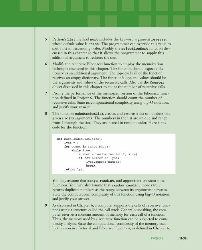
5 Python’s list method sort includes the keyword argument reverse,whose default value is False. The programmer can override this value tosort a list in descending order. Modify the selectionSort function dis-cussed in this chapter so that it allows the programmer to supply thisadditional argument to redirect the sort.

6 Modify the recursive Fibonacci function to employ the memoizationtechnique discussed in this chapter. The function should expect a dic-tionary as an additional argument. The top-level call of the functionreceives an empty dictionary. The function’s keys and values should bethe arguments and values of the recursive calls. Also use the Counterobject discussed in this chapter to count the number of recursive calls.

7 Profile the performance of the memoized version of the Fibonacci func-tion defined in Project 6. The function should count the number ofrecursive calls. State its computational complexity using big-O notation,and justify your answer.

8 The function makeRandomList creates and returns a list of numbers of agiven size (its argument). The numbers in the list are unique and rangefrom 1 through the size. They are placed in random order. Here is thecode for the function:

defƒmakeRandomList(size):ƒƒƒƒlystƒ=ƒ[]ƒƒƒƒforƒcountƒinƒrange(size):ƒƒƒƒƒƒƒƒwhileƒTrue:ƒƒƒƒƒƒƒƒƒƒƒƒnumberƒ=ƒrandom.randint(1,ƒsize)ƒƒƒƒƒƒƒƒƒƒƒƒif notƒnumberƒinƒlyst:ƒƒƒƒƒƒƒƒƒƒƒƒƒƒƒƒlyst.append(number)ƒƒƒƒƒƒƒƒƒƒƒƒƒƒƒƒbreakƒƒƒƒreturnƒlyst

You may assume that range, randint, and append are constant timefunctions. You may also assume that random.randint more rarelyreturns duplicate numbers as the range between its arguments increases.State the computational complexity of this function using big-O notation,and justify your answer.

9 As discussed in Chapter 6, a computer supports the calls of recursive func-tions using a structure called the call stack. Generally speaking, the com-puter reserves a constant amount of memory for each call of a function.Thus, the memory used by a recursive function can be subjected to com-plexity analysis. State the computational complexity of the memory usedby the recursive factorial and Fibonacci functions, as defined in Chapter 6.


10 The function that draws c-curves, and which was discussed in Chapter 7,has two recursive calls. Here is the code:

defƒcCurve(t,ƒx1,ƒy1,ƒx2,ƒy2,ƒlevel):

ƒƒƒdefƒdrawLine(x1,ƒy1,ƒx2,ƒy2):ƒƒƒƒƒƒ“””Drawsƒaƒlineƒsegmentƒbetweenƒtheƒendpoints.”””ƒƒƒƒƒƒt.up()ƒƒƒƒƒƒt.goto(x1,ƒy1)ƒƒƒƒƒƒt.down()ƒƒƒƒƒƒt.goto(x2,ƒy2)ƒƒƒƒƒƒƒƒƒifƒlevelƒ==ƒ0:ƒƒƒƒƒƒdrawLine(x1,ƒy1,ƒx2,ƒy2)ƒƒƒelse:ƒƒƒƒƒƒxmƒ=ƒ(x1ƒ+ƒx2ƒ+ƒy1ƒ-ƒy2)ƒ//ƒ2ƒƒƒƒƒƒymƒ=ƒ(x2ƒ+ƒy1ƒ+ƒy2ƒ-ƒx1)ƒ//ƒ2ƒƒƒƒƒƒcCurve(t,ƒx1,ƒy1,ƒxm,ƒym,ƒlevelƒ-ƒ1)ƒƒƒƒƒƒcCurve(t,ƒxm,ƒym,ƒx2,ƒy2,ƒlevelƒ-ƒ1)

You can assume that the function drawLine runs in constant time.State the computational complexity of the cCurve function, in termsof the level, using big-O notation. Also, draw a call tree for a call ofthis function with a level of 3.

complexity analysis - cengage learning

Documents