Complexity of Representation and Inference inCompositional Models with Part Sharing

Alan L. YuilleDepts. of Statistics, Computer Science & Psychology

University of California, Los Angelesyuille@stat.ucla.edu

Roozbeh MottaghiDepartment of Computer Science

University of California, Los Angelesroozbehm@cs.ucla.edu

Abstract

This paper describes serial and parallel compositional models of multiple objectswith part sharing. Objects are built by part-subpart compositions and expressedin terms of a hierarchical dictionary of object parts. These parts are representedon lattices of decreasing sizes which yield an executive summary description. Wedescribe inference and learning algorithms for these models. We analyze the com-plexity of this model in terms of computation time (for serial computers) and num-bers of nodes (e.g., ”neurons”) for parallel computers. In particular, we computethe complexity gains by part sharing and its dependence on how the dictionaryscales with the level of the hierarchy. We explore three regimes of scaling be-havior where the dictionary size (i) increases exponentially with the level, (ii) isdetermined by an unsupervised compositional learning algorithm applied to realdata, (iii) decreases exponentially with scale. This analysis shows that in someregimes the use of shared parts enables algorithms which can perform inferencein time linear in the number of levels for an exponential number of objects. Inother regimes part sharing has little advantage for serial computers but can givelinear processing on parallel computers.

1 Introduction

A fundamental problem of vision is how to deal with the enormous complexity of images and visualscenes 1. The total number of possible images is almost infinitely large [8]. The number of objectsis also huge and has been estimated at around 30,000 [2]. How can a biological, or artificial, visionsystem deal with this complexity? For example, considering the enormous input space of imagesand output space of objects, how can humans interpret images in less than 150 msec [16]?

There are three main issues involved. Firstly, how can a visual system be designed so that it canefficiently represent large classes of objects, including their parts and subparts? Secondly, how canthe visual system be designed so that it can rapidly infer which object, or objects, are present in aninput image and the positions of their subparts? And, thirdly, how can this representation be learntin an unsupervised, or weakly supervised fashion? In short, what visual architectures enable us toaddress these three issues?

Many considerations suggest that visual architectures should be hierarchical. The structure of mam-malian visual systems is hierarchical with the lower levels (e.g., in areas V1 and V2) tuned to smallimage features while the higher levels (i.e. in area IT) are tuned to objects 2. Moreover, as ap-preciated by pioneers such as Fukushima [5], hierarchical architectures lend themselves naturally to

1Similar complexity issues will arise for other perceptual and cognitive modalities.2But just because mammalian visual systems are hierarchical does not necessarily imply that this is the best

design for computer vision systems.

efficient representations of objects in terms of parts and subparts which can be shared between manyobjects. Hierarchical architectures also lead to efficient learning algorithms as illustrated by deepbelief learning and others [7]. There are many varieties of hierarchical models which differ in detailsof their representations and their learning and inference algorithms [14, 7, 15, 1, 13, 18, 10, 3, 9].But, to the best of our knowledge, there has been no detailed study of their complexity properties.

This paper provides a mathematical analysis of compositional models [6], which are a subclass of thehierarchical models. The key idea of compositionality is to explicitly represent objects by recursivecomposition from parts and subparts. This gives rise to natural learning and inference algorithmswhich proceed from sub-parts to parts to objects (e.g., inference is efficient because a leg detectorcan be used for detecting the legs of cows, horses, and yaks). The explicitness of the object rep-resentations helps quantify the efficiency of part-sharing and make mathematical analysis possible.The compositional models we study are based on the work of L. Zhu and his collaborators [19, 20]but we make several technical modifications including a parallel re-formulation of the models. Wenote that in previous papers [19, 20] the representations of the compositional models were learnt inan unsupervised manner, which relates to the memorization algorithms of Valiant [17]. This paperdoes not address learning but instead explores the consequence of the representations which werelearnt.

Our analysis assumes that objects are represented by hierarchical graphical probability models 3

which are composed from more elementary models by part-subpart compositions. An object – agraphical model with H levels – is defined as a composition of r parts which are graphical modelswithH− 1 levels. These parts are defined recursively in terms of subparts which are represented bygraphical models of increasingly lower levels. It is convenient to specify these compositional modelsin terms of a set of dictionaries {Mh : h = 1, .., ,H} where the level-h parts in dictionaryMh arecomposed in terms of level-h − 1 parts in dictionary Mh−1. The highest level dictionaries MHrepresent the set of all objects. The lowest level dictionariesM1 represent the elementary featuresthat can be measured from the input image. Part-subpart composition enables us to construct avery large number of objects by different compositions of elements from the lowest-level dictionary.It enables us to perform part-sharing during learning and inference, which can lead to enormousreductions in complexity, as our mathematical analysis will show.

There are three factors which enable computational efficiency. The first is part-sharing, as describedabove, which means that we only need to perform inference on the dictionary elements. The secondis the executive-summary principle. This principle allows us to represent the state of a part coarselybecause we are also representing the state of its subparts (e.g., an executive will only want to knowthat ”there is a horse in the field” and will not care about the precise positions of its legs). Forexample, consider a letter T which is composed of a horizontal and vertical bar. If the positionsof these two bars are specified precisely, then we can specify the position of the letter T morecrudely (sufficient for it to be ”bound” to the two bars). This relates to Lee and Mumford’s high-resolution buffer hypothesis [11] and possibly to the experimental finding that neurons higher upthe visual pathway are tuned to increasingly complex image features but are decreasingly sensitiveto spatial position. The third factor is parallelism which arises because the part dictionaries canbe implemented in parallel, essentially having a set of receptive fields, for each dictionary element.This enables extremely rapid inference at the cost of a larger, but parallel, graphical model.

The compositional section (2) introduces the key ideas. Section (3) describes the inference algo-rithms for serial and parallel implementations. Section (4) performs a complexity analysis andshows potential exponential gains by using compositional models.

2 The Compositional Models

Compositional models are based on the idea that objects are built by compositions of parts which,in turn, are compositions of more elementary parts. These are built by part-subpart compositions.

3These graphical models contain closed loops but with restricted maximal clique size.

2

(a) (b)

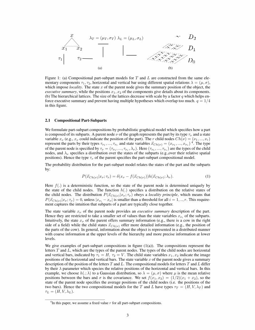
Figure 1: (a) Compositional part-subpart models for T and L are constructed from the same ele-mentary components τ1, τ2, horizontal and vertical bar using different spatial relations λ = (µ, σ),which impose locality. The state x of the parent node gives the summary position of the object, theexecutive summary, while the positions x1, x2 of the components give details about its components.(b) The hierarchical lattices. The size of the lattices decrease with scale by a factor q which helps en-force executive summary and prevent having multiple hypotheses which overlap too much. q = 1/4in this figure.

2.1 Compositional Part-Subparts

We formulate part-subpart compositions by probabilistic graphical model which specifies how a partis composed of its subparts. A parent node ν of the graph represents the part by its type τν and a statevariable xν (e.g., xν could indicate the position of the part). The r child nodes Ch(ν) = (ν1, ..., νr)represent the parts by their types τν1 , ..., τνr and state variables ~xCh(ν) = (xν1 , ..., xνr )

4. The typeof the parent node is specified by τν = (τν1 , ..., τνr , λν). Here (τν1 , ..., τνr ) are the types of the childnodes, and λν specifies a distribution over the states of the subparts (e.g.,over their relative spatialpositions). Hence the type τν of the parent specifies the part-subpart compositional model.

The probability distribution for the part-subpart model relates the states of the part and the subpartsby:

P (~xCh(ν)|xν ; τν) = δ(xν − f(~xCh(ν)))h(~xCh(ν);λν). (1)

Here f(.) is a deterministic function, so the state of the parent node is determined uniquely bythe state of the child nodes. The function h(.) specifies a distribution on the relative states ofthe child nodes. The distribution P (~xCh(ν)|xν ; τν) obeys a locality principle, which means thatP (~xCh(ν)|xν ; τν) = 0, unless |xνi − xν | is smaller than a threshold for all i = 1, .., r. This require-ment captures the intuition that subparts of a part are typically close together.

The state variable xν of the parent node provides an executive summary description of the part.Hence they are restricted to take a smaller set of values than the state variables xνi of the subparts.Intuitively, the state xν of the parent offers summary information (e.g., there is a cow in the rightside of a field) while the child states ~xCh(ν) offer more detailed information (e.g., the position ofthe parts of the cow). In general, information about the object is represented in a distributed mannerwith coarse information at the upper levels of the hierarchy and more precise information at lowerlevels.

We give examples of part-subpart compositions in figure (1(a)). The compositions represent theletters T and L, which are the types of the parent nodes. The types of the child nodes are horizontaland vertical bars, indicated by τ1 = H, τ2 = V . The child state variables x1, x2 indicate the imagepositions of the horizontal and vertical bars. The state variable x of the parent node gives a summarydescription of the position of the letters T andL. The compositional models for letters T andL differby their λ parameter which species the relative positions of the horizontal and vertical bars. In thisexample, we choose h(.;λ) to a Gaussian distribution, so λ = (µ, σ) where µ is the mean relativepositions between the bars and σ is the covariance. We set f(x1, x2) = (1/2)(x1 + x2), so thestate of the parent node specifies the average positions of the child nodes (i.e. the positions of thetwo bars). Hence the two compositional models for the T and L have types τT = (H,V, λT ) andτL = (H,V, λL).

4In this paper, we assume a fixed value r for all part-subpart compositions.

3

OR

Figure 2: Left Panel: Two part-subpart models. Center Panel: Combining two part-subpart modelsby composition to make a higher level model. Right Panel: Some examples of the shapes that canbe generated by different parameters settings λ of the distribution.

2.2 Models of Object Categories

An object category can be modeled by repeated part-subpart compositions. This is illustrated infigure (2) where we combine T ’s and L’s with other parts to form more complex objects. Moregenerally, we can combine part-subpart compositions into bigger structures by treating the parts assubparts of higher order parts.

More formally, an object category of type τH is represented by a probability distribution defined overa graph V . This graph has a hierarchical structure with levels h ∈ {0, ...,H}, where V =

⋃Hh=0 Vh.

Each object has a single, root node, at level-H (i.e. VH contains a single node). Any node ν ∈ Vh(for h > 0) has r children nodes Ch(ν) in Vh−1 indexed by (ν1, ..., νr). Hence there are rH−hnodes at level-h (i.e. |Vh| = rH−h).

At each node ν there is a state variable xν which indicates spatial position and type τν . The type τHof the root node indicates the object category and also specifies the types of its parts.

The position variables xν take values in a set of lattices {Dh : h = 0, ...,H}, so that a level-h node,ν ∈ Vh, takes position xν ∈ Dh. The leaf nodes V0 of the graph take values on the image latticeD0.The lattices are evenly spaced and the number of lattice points decreases by a factor of q < 1 foreach level, so |Dh| = qh|D0|, see figure (1(b)). This decrease in number of lattice points imposesthe executive summary principle. The lattice spacing is designed so that parts do not overlap. Athigher levels of the hierarchy the parts cover larger regions of the image and so the lattice spacingmust be larger, and hence the number of lattice points smaller, to prevent overlapping 5.

The probability model for an object category of type τH is specified by products of part-subpartrelations:

P (~x|τH) =∏

ν∈V/V0P (~xCh(ν)|xν ; τν)U(xH). (2)

Here U(xH) is the uniform distribution.

2.3 Multiple Object Categories, Shared Parts, and Hierarchical Dictionaries

Now suppose we have a set of object categories τH ∈ H, each of which can be expressed by anequation such as equation (2). We assume that these objects share parts. To quantify the amount ofpart sharing we define a hierarchical dictionary {Mh : h = 0, ...,H}, whereMh is the dictionaryof parts at level h. This gives an exhaustive set of the parts of this set of the objects, at all levelsh = 0, ...,H. The elements of the dictionary Mh are composed from elements of the dictionaryMh−1 by part-subpart compositions 6.

This gives an alternative way to think of object models. The type variable τν of a node at level h(i.e. in Vh) indexes an element of the dictionary Mh. Hence objects can be encoded in terms ofthe hierarchical dictionary. Moreover, we can create new objects by making new compositions fromexisting elements of the dictionaries.

5Previous work [20, 19] was not formulated on lattices and used non-maximal suppression to achieve thesame effect.

6The unsupervised learning algorithm in [19] automatically generates this hierarchical dictionary.

4

2.4 The Likelihood Function and the Generative Model

To specify a generative model for each object category we proceed as follows. The prior specifies adistribution over the positions and types of the leaf nodes of the object model. Then the likelihoodfunction is specified in terms of the type at the leaf nodes (e.g., if the leaf node is a vertical bar, thenthere is a high probability that the image has a vertical edge at that position).

More formally, the prior P (~x|τH), see equation (2), specifies a distribution over a set of points L ={xν : ν ∈ V0} (the leaf nodes of the graph) and specifies their types {τν : ν ∈ V0}. These pointsare required to lie on the image lattice (e.g., xν ∈ D0). We denote this as {(x, τ(x)) : x ∈ L} whereτ(x) is specified in the natural manner (i.e. if x = xν then τ(x) = τν). We specify distributionsP (I(x)|τ(x)) for the probability of the image I(x) at x conditioned on the type of the leaf node.We specify a default probability P (I(x)|τ0) at positions x where there is no leaf node of the object.

This gives a likelihood function for the states ~x = {xν ∈ V} of the object model in terms of theimage I = {I(x) : x ∈ D0}:

P (I|~x) =∏x∈L

P (I(x)|τ(x))×∏

x∈D0/LP (I(x)|τ0). (3)

The likelihood and the prior, equations (3,2), give a generative model for each object category.

We can extend this in the natural manner to give generative models or two, or more, objects in theimage provided they do not overlap. Intuitively, this involves multiple sampling from the prior todetermine the types of the lattice pixels, followed by sampling from P (I(x)|τ) at the leaf nodes todetermine the image I. Similarly, we have a default background model for the entire image if noobject is present:

PB(I) =∏x∈D0

P (I(x)|τ0). (4)

3 Inference by Dynamic Programming

The inference task is to determine which objects are present in the image and to specify their po-sitions. This involves two subtasks: (i) state estimation, to determine the optimal states of a modeland hence the position of the objects and its parts, and (ii) model selection, to determine whetherobjects are present or not. As we will show, both tasks can be reduced to calculating and comparinglog-likelihood ratios which can be performed efficiently using dynamic programming methods.

We will first describe the simplest case which consists of estimating the state variables of a singleobject model and using model selection to determine whether the object is present in the image and,if so, how many times. Next we show that we can perform inference and model selection for multipleobjects efficiently by exploiting part sharing (using hierarchical dictionaries). Finally, we show howthese inference tasks can be performed even more efficiently using a parallel implementation. Westress that we are performing exact inference and no approximations are made. We are simplyexploiting part-sharing so that computations required for performing inference for one object can bere-used when performing inference for other objects.

3.1 Inference Tasks: State Detection and Model Selection

We first describe a standard dynamic programming algorithm for finding the optimal state of a singleobject category model. Then we describe how the same computations can be used to perform modelselection and to the detection and state estimation if the object appears multiple times in the image(non-overlapping).

Consider performing inference for a single object category model defined by equations (2,3). Tocalculate the MAP estimate of the state variables requires computing ~x∗ = argmax~x{logP (I|~x) +logP (~x; τH)}. By subtracting the constant term logPB(I) from the righthand side, we can re-express this as estimating:

~x∗ = argmax~x{∑x∈L

logP (I(x)|τ(x))P (I(x)|τ0)

+∑ν

logP (~xCh(ν)|xν ; τν) + logU(xH)}. (5)

5

Figure 3: Left Panel: The feedforward pass propagates hypotheses up to the highest level wherethe best state is selected. Center Panel: Feedback propagates information from the top node disam-biguating the middle level nodes. Right Panel: Feedback from the middle level nodes propagatesback to the input layer to resolve ambiguities there. This algorithm rapidly estimates the top-levelexecutive summary description in a rapid feed-forward pass. The top-down pass is required to allowhigh-level context to eliminate false hypotheses at the lower levels– ”high-level tells low-level tostop gossiping”.

Here L denotes the positions of the leaf nodes of the graph, which must be determined duringinference.

We estimate ~x∗ by performing dynamic programming. This involves a bottom-up pass which recur-sively computes quantities φ(xh, τh) = argmax~x/xh{log P (I|~x)

PB(I) + logP (~x; τh)} by the formula:

φ(xh, τh) = max~xCh(ν)

{r∑i=1

φ(xνi , τνi) + logP (~xCh(ν)|x∗ν , τν)}. (6)

We refer to φ(xh, τh) as the local evidence for part τh with state xh (after maximizing over the statesof the lower parts of the graphical model). This local evidence is computed bottom-up. We call thisthe local evidence because it ignores the context evidence for the part which will be provided duringtop-down processing (i.e. that evidence for other parts of the object, in consistent positions, willstrengthen the evidence for this part).

The bottom-up pass outputs the global evidence φ(xH, τH) for object category τH at position xH.We can detect the most probable state of the object by computing x∗H = argmaxφ(xH, τH). Thenwe can perform the top-down pass of dynamic programming to estimate the most probable states ~x∗of the entire model by recursively performing:

~x∗Ch(ν) = arg max~xCh(ν)

{r∑i=1

φ(xνi , τνi) + logP (~xCh(ν)|x∗ν , τν)}. (7)

This outputs the most probable state of the object in the image. Note that the bottom-up process firstestimates the optimal ”executive summary” description of the object (x∗H) and only later determinesthe optimal estimates of the lower-level states of the object in the top-down pass. Hence, the algo-rithm is faster at detecting that there is a cow in the right side of the field (estimated in the bottom-uppass) and is slower at determining the position of the feet of the cow (estimated in the top-downpass). This is illustrated in figure (3).

Importantly, we only need to perform slight extensions of this algorithm to compute significantlymore. First, we can perform model selection – to determine if the object is present in the image – bydetermining if φ(x∗H, τH) > T , where T is a threshold. This is because, by equation (5), φ(x∗H, τH)is the log-likelihood ratio of the probability that the object is present at position x∗H compared to theprobability that the corresponding part of the image is generated by the background image modelPB(.). Secondly, we can compute the probability that the object occurs several times in the image,by computing the set {xH : φ(x∗H, τH) > T , to compute the ”executive summary” descriptionsfor each object (e.g., the coarse positions of each object). We then perform the top-down passinitialized at each coarse position (i.e. at each point of the set described above) to determine theoptimal configuration for the states of the objects. Hence, we can reuse the computations requiredto detect a single object in order to detect multiple instances of the object (provided there are no

6

a b

A

b c

B

b

a b

A

c

B

Or

Figure 4: Sharing. Left Panel: Two Level-2 models A and B which share Level-1 model b as asubpart. Center Panel: Level-1 model b. Inference computation only requires us to do inferenceover model b once, and then it can be used to computer the optimal states for models A and B.Right Panel: Note that is we combine modelsA andB by a root OR node then we obtain a graphicalmodel for both objects. This model has a closed loop which would seem to make inference morechallenging. But by exploiting the shape part we can do inference optimally despite the closed loop.Inference can be done on the dictionaries, far right.

overlaps)7. The number of objects in the image is determined by the log-likelihood ratio test withrespect to the background model.

3.2 Inference on Multiple Objects by Part Sharing using the Hierarchical Dictionaries

Now suppose we want to detect instances of many object categories τH ∈MH simultaneously. Wecan exploit the shared parts by performing inference using the hierarchical dictionaries.

The main idea is that we need to compute the global evidence φ(xH, τH) for all objects τH ∈ MHand at all positions xH in the top-level lattice. These quantities could be computed separately foreach object by performing the bottom-up pass, specified by equation (6), for each object. But thisis wasteful because the objects share parts and so we would be performing the same computationsmultiple times. Instead we can perform all the necessary computations more efficiently by workingdirectly with the hierarchical dictionaries.

More formally, computing the global evidence for all object models and at all positions is specifiedas follows.

Let D∗H = {xH ∈ DH s.t. maxτH∈MH

φ(xH, τH) > TH},

For xH ∈ D∗H, let τ∗H(xH) = arg maxτH∈MH

φ(xH, τH),

Detect ~x∗/xH = arg max~x/xH{log P (I|~x)

PB(I)+ logP (~x; τH∗(xH))} for all xH ∈ D∗H. (8)

All these calculations can be done efficiently using the hierarchical dictionaries (except for the maxand argmax tasks at levelHwhich must be done separately). Recalling that each dictionary elementat level h is composed, by part-subpart composition, of dictionary elements at level h − 1. Hencewe can apply the bottom-up update rule in equation (6) directly to the dictionary elements. This isillustrated in figure (4). As analyzed in the next section, this can yield major gains in computationalcomplexity.

Once the global evidences for each object model have been computed at each position (in the toplattice) we can perform winner-take-all to estimate the object model which has largest evidenceat each position. Then we can apply thresholding to see if it passes the log-likelihood ratio testcompared to the background model. If it does pass this log-likelihood test, then we can use thetop-down pass of dynamic programming, see equation (7), to estimate the most probable state of allparts of the object model.

7Note that this is equivalent to performing optimal inference simultaneously over a set of different generativemodels of the image, where one model assumes that there is one instance of the object in the image, anothermodels assumes there are two, and so on.

7

We note that we are performing exact inference over multiple object models at the same time. Thisis perhaps un-intuitive to some readers because this corresponds to doing exact inference over aprobability model which can be expressed as a graph with a large number of closed loops, seefigure (4). But the main point is that part-sharing enables us share inference efficiently betweenmany models.

The only computation which cannot be performed by dynamic programming are the max andargmax tasks at level H , see top line of equation (8). These are simple operations and requireorder MH × |DH| calculations. This will usually be a small number, compared to the complexityof other computations. But this will become very large if there are a large number of objects, as wewill discuss in section (4).

3.3 Parallel Formulation and Inference Algorithm

Finally, we observe that all the computations required for performing inference on multiple objectscan be parallelized. This requires computing the quantities in equation (8).

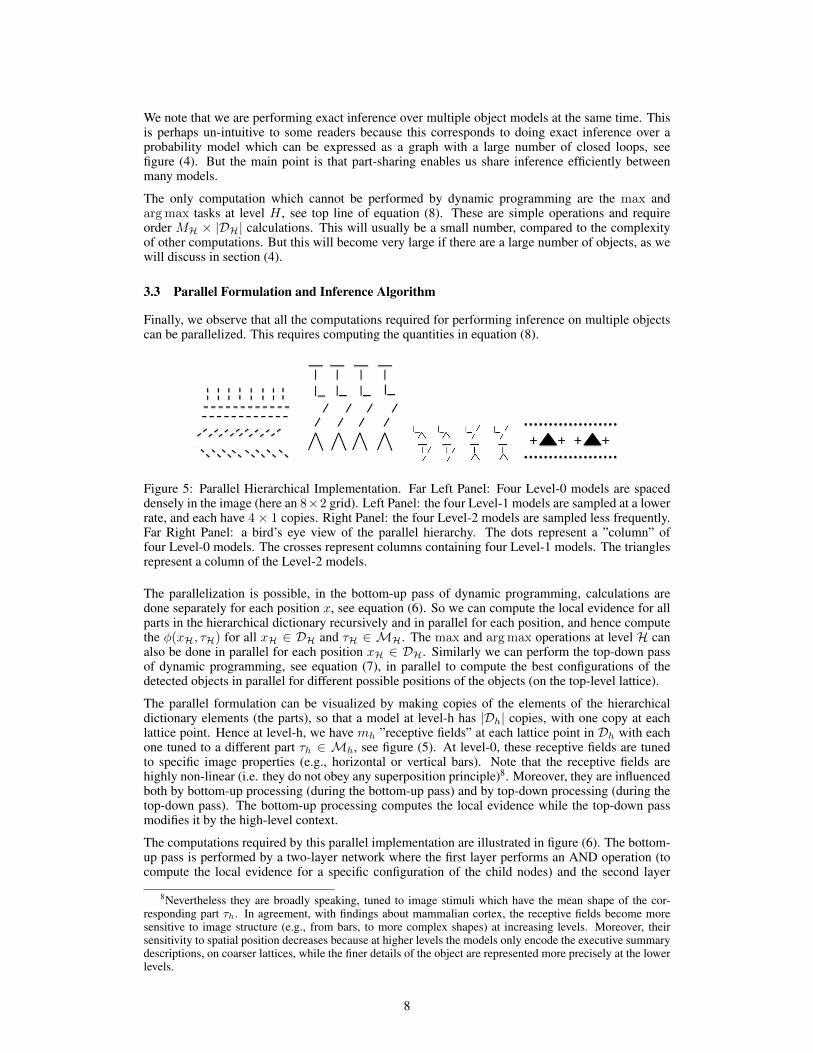
Figure 5: Parallel Hierarchical Implementation. Far Left Panel: Four Level-0 models are spaceddensely in the image (here an 8×2 grid). Left Panel: the four Level-1 models are sampled at a lowerrate, and each have 4× 1 copies. Right Panel: the four Level-2 models are sampled less frequently.Far Right Panel: a bird’s eye view of the parallel hierarchy. The dots represent a ”column” offour Level-0 models. The crosses represent columns containing four Level-1 models. The trianglesrepresent a column of the Level-2 models.

The parallelization is possible, in the bottom-up pass of dynamic programming, calculations aredone separately for each position x, see equation (6). So we can compute the local evidence for allparts in the hierarchical dictionary recursively and in parallel for each position, and hence computethe φ(xH, τH) for all xH ∈ DH and τH ∈ MH. The max and argmax operations at level H canalso be done in parallel for each position xH ∈ DH. Similarly we can perform the top-down passof dynamic programming, see equation (7), in parallel to compute the best configurations of thedetected objects in parallel for different possible positions of the objects (on the top-level lattice).

The parallel formulation can be visualized by making copies of the elements of the hierarchicaldictionary elements (the parts), so that a model at level-h has |Dh| copies, with one copy at eachlattice point. Hence at level-h, we have mh ”receptive fields” at each lattice point in Dh with eachone tuned to a different part τh ∈ Mh, see figure (5). At level-0, these receptive fields are tunedto specific image properties (e.g., horizontal or vertical bars). Note that the receptive fields arehighly non-linear (i.e. they do not obey any superposition principle)8. Moreover, they are influencedboth by bottom-up processing (during the bottom-up pass) and by top-down processing (during thetop-down pass). The bottom-up processing computes the local evidence while the top-down passmodifies it by the high-level context.

The computations required by this parallel implementation are illustrated in figure (6). The bottom-up pass is performed by a two-layer network where the first layer performs an AND operation (tocompute the local evidence for a specific configuration of the child nodes) and the second layer

8Nevertheless they are broadly speaking, tuned to image stimuli which have the mean shape of the cor-responding part τh. In agreement, with findings about mammalian cortex, the receptive fields become moresensitive to image structure (e.g., from bars, to more complex shapes) at increasing levels. Moreover, theirsensitivity to spatial position decreases because at higher levels the models only encode the executive summarydescriptions, on coarser lattices, while the finer details of the object are represented more precisely at the lowerlevels.

8

Bottom Up Top Down

Figure 6: Parallel implementation of Dynamic Programming. The left part of the figure showsthe bottom-up pass of dynamic programming. The local evidence for the parent node is obtained bytaking the maximum of the scores of the Cr possible states of the child nodes. This can be computedby a two-layer network where the first level computes the scores for all Cr child node states, whichcan be done in parallel, and the second level compute the maximum score. This is like an ANDoperation followed by an OR. The top-down pass requires the parent node to select which of the Crchild configurations gave the maximum score, and suppressing the other configurations.

performs an OR, or max operation, to determine the local evidence (by max-ing over the possiblechild configurations)9. The top-down pass only has to perform an argmax computation to determinewhich child configuration gave the best local evidence.

4 Complexity Analysis

We now analyze the complexity of the inference algorithms for performing the tasks. Firstly, weanalyze complexity for a single object (without part-sharing). Secondly, we study the complexityfor multiple objects with shared parts. Thirdly, we consider the complexity of the parallel imple-mentation.

The complexity is expressed in terms of the following quantities: (I) The size |D0| of the image.(II) The scale decrease factor q (enabling executive summary). (III) The number H of levels of thehierarchy. (IV) The sizes {|Mh| : h = 1, ...,H} of the hierarchical dictionaries. (V) The number rof subparts of each part. (VI) The number Cr of possible part-subpart configurations.

4.1 Complexity for Single Objects and Ignoring Part Sharing

This section estimates the complexity of inference Nso for a single object and the complexity Nmofor multiple objects when part sharing is not used. These results are for comparison to the complex-ities derived in the following section using part sharing.

The inference complexity for a single object requires computing: (i) the number Nbu of compu-tations required by the bottom-up pass, (ii) the number Nms of computations required by modelselection at the top-level of the hierarchy, and (iii) the number Ntd of computations required by thetop-down pass.

The complexity Nbu of the bottom-up pass can be computed from equation (6). This requires a totalof Cr computations for each position xν for each level-h node. There are rH−h nodes at level h andeach can take |D0|qh positions. This gives a total of |D0|CrqhrH−h computations at level h. Thiscan be summed over all levels to yield:

Nbu =

H∑h=1

|D0|CrrH(q/r)h = |D0|CrrHH∑h=1

(q/r)h = |D0|CrqrH−1

1− q/r{1− (q/r)H}. (9)

Observe that the main contributions to Nbu come from the first few levels of the hierarchy becausethe factors (q/r)h decrease rapidly with h. This calculation uses

∑Hh=1 x

h = x(1−xH)1−x . For largeH

we can approximate Nbu by |D0|Cr qrH−1

1−q/r (because (q/r)H will be small).

9Note that other hierarchical models, including bio-inspired ones, use similar operations but motivated bydifferent reasons.

9

We calculate Nms = q|H||D0| for the complexity of model selection (which only requires thresh-olding at every point on the top-level lattice).

The complexity Ntd of the top-down pass is computed from equation (7). At each level thereare r|H|−h nodes and we must compute Cr computations for each. This yields complexity of∑|H|h=1 Crr

|H|−h for each possible root node. There are at most q|H||D0| possible root nodes (de-pending on the results of the model selection stage). This yields an upper bound:

Ntd ≤ |D0|Crq|H|r|H|−1

1− 1/r{1− 1

r|H−1|}. (10)

Clearly the complexity is dominated by the complexity Nbu of the bottom-up pass. For simplicity,we will bound/approximate this by:

Nso = |D0|CrqrH−1

1− q/r (11)

Now suppose we perform inference for multiple objects simultaneously without exploiting sharedparts. In this case the complexity will scale linearly with the number |MH| of objects. This givesus complexity:

Nmo = |MH||D0|CrqrH−1

1− q/r (12)

4.2 Computation with Shared Parts in Series and in Parallel

This section computes the complexity using part sharing. Firstly, for the standard serial implemen-tation of part sharing. Secondly, for the parallel implementation.

Now suppose we perform inference on many objects with part sharing using a serial computer.This requires performing computations over the part-subpart compositions between elements of thedictionaries. At level h there are |Mh| dictionary elements. Each can take |Dh| = qh|D| possiblestates. The bottom-up pass requires performing Cr computations for each of them. This gives atotal of

∑Hh=1 |Mh|Cr|D0|qh = |D0|Cr

∑Hh=1 |Mh|qh computations for the bottom-up process.

The complexity of model selection is |D0|qH × (H + 1) (this is between all the objects, and thebackground model, at all points on the top lattice). As in the previous section, the complexity of thetop-down process is less than the complexity of the bottom-up process. Hence the complexity formultiple objects using part sharing is given by:

Nps = |D0|CrH∑h=1

|Mh|qh. (13)

Next consider the parallel implementation. In this case almost all of the computations are performedin parallel and so the complexity is now expressed in terms of the number of ”neurons” required toencode the dictionaries, see figure (5). This is specified by the total number of dictionary elementsmultiplied by the number of spatial copies of them:

Nn =

H∑h=1

|Mh|qh|D0|. (14)

The computation, both the forward and backward passes of dynamic programming, are linear in thenumber H of levels. We only need to perform the computations illustrated in figure (6) between alladjacent levels.

Hence the parallel implementation gives speed which is linear in H at the cost of a possibly largenumber Nn of ”neurons” and connections between them.

4.3 Advantages of Part Sharing in Different Regimes

The advantages of part-sharing depend on how the number of parts |Mh| scales with the level hof the hierarchy. In this section we consider three different regimes: (I) The exponential growth

10

regime where the size of the dictionaries increases exponentially with the level h. (II) The empiricalgrowth regime where we use the size of the dictionaries found experimentally by compositionallearning [19]. (III) The exponential decrease regime where the size of the dictionaries decreasesexponentially with level h. For all these regimes we compare the advantages of the serial and parallelimplementations using part sharing by comparison to the complexity results without sharing.

Exponential growth of dictionaries is a natural regime to consider. It occurs when subparts areallowed to combine with all other subparts (or a large fraction of them) which means that the numberof part-subpart compositions is polynomial in the number of subparts. This gives exponential growthin the size of the dictionaries if it occurs at different levels (e.g., consider the enormous number ofobjects that can be built using lego).

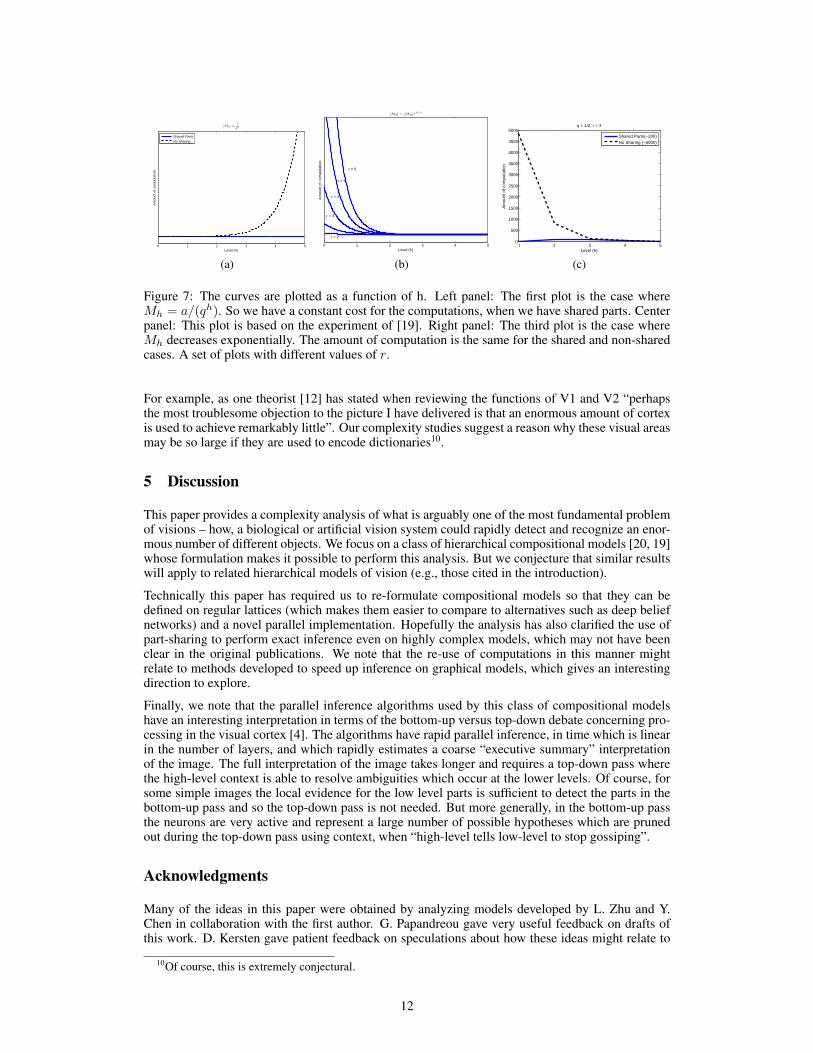
An interesting special case of the exponential growth regime is when |Mh| scales like 1/qh, seefigure (7)(left panel). In this case the complexity of computation for serial part-sharing, and thenumber of neurons required for parallel implementation, scales only with the number of levels H.This follows from equations (13,14). But nevertheless the number of objects that can be detectedscales exponentially as qM. By contrast, the complexity of inference without part-sharing scalesexponentially with q, see equation (12, because we have to perform a fixed number of computations,given by equation (11), for each of an exponential number of objects. This is summarized by thefollowing result.

Result 1: If the number of shared parts scales exponentially by |Mh| ∝ 1qh

then we can performinference for order qH objects using part sharing in time linear in H, or with a number of neu-rons linear in H for parallel implementation. By contrast, inference without part-sharing requiresexponential complexity.

To what extent is exponential growth a reasonable assumption for real world objects? This motivatesus to study the empirical growth regime using the dictionaries obtained by the compositional learningexperiments reported in [19]. In these experiments, the size of the dictionaries increased rapidly atthe lower levels (i.e. small h) and then decreased at higher levels (roughly consistent with thefindings of psychophysical studies – Biederman, personal communication). For these ”empiricaldictionaries” we plot the growth, and the number of computations at each level of the hierarchy, infigure (7)(center panel). This shows complexity which roughly agrees with the exponential growthmodel. This can be summarized by the following result:

Result 2: If |Mh| grows slower than 1/qh and if |Mh| < rH−h then there are gains due to partsharing using serial and parallel computers. This is illustrated in figure (7)(center panel) based onthe dictionaries found by unsupervised computational learning [19]. In parallel implementations,computation is linear inH while requiring a limited number of nodes (”neurons”).

Finally we consider the exponential decrease regime. To motivate this regime, suppose that thedictionaries are used to model image appearance, by contrast to the dictionaries based on geometricalfeatures such as bars and oriented edges (as used in [19]). It is reasonable to assume that there are alarge number of low-level dictionaries used to model the enormous variety of local intensity patterns.The number of higher-level dictionaries can decrease because they can be used to capture a crudersummary description of a larger image region, which is another instance of the executive summaryprinciple. For example, the low-level dictionaries could be used to provide detailed modeling ofthe local appearance of a cat, or some other animal, while the higher-level dictionaries could givesimpler descriptions like ”cat-fur” or ”dog-fur” or simply ”fur”. In this case, it is plausible that thesize of the dictionaries decreases exponentially with the level h. The results for this case emphasizethe advantages of parallel computing.

Result 3: If |Mh| = rH−h then there is no gain for part sharing if serial computers are used, seefigure (7)(right panel). Parallel implementations can do inference in time which is linear in H butrequire an exponential number of nodes (”neurons”).

Result 3 may appear negative at first glance even for the parallel version since it requires an expo-nentially large number of neurons required to encode the lower level dictionaries. But it may relateto one of the more surprising facts about the visual cortex in monkeys and humans – namely that thefirst two visual areas, V1 and V2, where low-level dictionaries would be implemented are enormouscompared to the higher levels such as IT where object detection takes places. Current models of V1and V2 mostly relegate it to being a large filter bank which seems paradoxical considering their size.

11

0 1 2 3 4 5Level (h)

|Mh| ∝1

qh

Am

ount

of c

ompu

tatio

n

Shared PartsNo Sharing

(a)

0 1 2 3 4 5Level (h)

|Mh| = |MH|rH−h

Am

ount

of c

ompu

tatio

n

r = 5

r = 3

r = 4

r = 6

r = 2

(b)

1 2 3 4 50

500

1000

1500

2000

2500

3000

3500

4000

4500

5000q = 1/2, r = 3

Level (h)

Am

ount

of c

ompu

tatio

n

Shared Parts(~200)No Sharing (~6000)

(c)

Figure 7: The curves are plotted as a function of h. Left panel: The first plot is the case whereMh = a/(qh). So we have a constant cost for the computations, when we have shared parts. Centerpanel: This plot is based on the experiment of [19]. Right panel: The third plot is the case whereMh decreases exponentially. The amount of computation is the same for the shared and non-sharedcases. A set of plots with different values of r.

For example, as one theorist [12] has stated when reviewing the functions of V1 and V2 “perhapsthe most troublesome objection to the picture I have delivered is that an enormous amount of cortexis used to achieve remarkably little”. Our complexity studies suggest a reason why these visual areasmay be so large if they are used to encode dictionaries10.

5 Discussion

This paper provides a complexity analysis of what is arguably one of the most fundamental problemof visions – how, a biological or artificial vision system could rapidly detect and recognize an enor-mous number of different objects. We focus on a class of hierarchical compositional models [20, 19]whose formulation makes it possible to perform this analysis. But we conjecture that similar resultswill apply to related hierarchical models of vision (e.g., those cited in the introduction).

Technically this paper has required us to re-formulate compositional models so that they can bedefined on regular lattices (which makes them easier to compare to alternatives such as deep beliefnetworks) and a novel parallel implementation. Hopefully the analysis has also clarified the use ofpart-sharing to perform exact inference even on highly complex models, which may not have beenclear in the original publications. We note that the re-use of computations in this manner mightrelate to methods developed to speed up inference on graphical models, which gives an interestingdirection to explore.

Finally, we note that the parallel inference algorithms used by this class of compositional modelshave an interesting interpretation in terms of the bottom-up versus top-down debate concerning pro-cessing in the visual cortex [4]. The algorithms have rapid parallel inference, in time which is linearin the number of layers, and which rapidly estimates a coarse “executive summary” interpretationof the image. The full interpretation of the image takes longer and requires a top-down pass wherethe high-level context is able to resolve ambiguities which occur at the lower levels. Of course, forsome simple images the local evidence for the low level parts is sufficient to detect the parts in thebottom-up pass and so the top-down pass is not needed. But more generally, in the bottom-up passthe neurons are very active and represent a large number of possible hypotheses which are prunedout during the top-down pass using context, when “high-level tells low-level to stop gossiping”.

Acknowledgments

Many of the ideas in this paper were obtained by analyzing models developed by L. Zhu and Y.Chen in collaboration with the first author. G. Papandreou gave very useful feedback on drafts ofthis work. D. Kersten gave patient feedback on speculations about how these ideas might relate to

10Of course, this is extremely conjectural.

12

the brain. The WCU program at Korea University, under the supervision of S-W Lee, gave peaceand time to develop these ideas.

References

[1] N. J. Adams and C. K. I. Williams. Dynamic trees for image modelling. Image and VisionComputing, 20(10):865–877, 2003.

[2] I. Biederman. Recognition-by-components: a theory of human image understanding. Psycho-logical Review, 94(2):115–147, Apr. 1987.

[3] E. Borenstein and S. Ullman. Class-specific, top-down segmentation. ECCV 2002, pages639–641, 2002.

[4] J. J. DiCarlo, D. Zoccolan, and N. C. Rust. How Does the Brain Solve Visual Object Recogni-tion? Neuron, 73(3):415–434, Feb. 2012.

[5] K. Fukushima. Neocognitron - a Hierarchical Neural Network Capable of Visual-PatternRecognition. Neural Networks, 1(2):119–130, 1988.

[6] S. Geman, D. Potter, and Z. Chi. Composition systems. Quarterly of Applied Mathematics,60(4):707–736, 2002.

[7] G. E. Hinton, S. Osindero, and Y. Teh. A fast learning algorithm for deep belief nets. NeuralComputation, 18:1527–54, 2006.

[8] D. Kersten. Predictability and redundancy of natural images. JOSA A, 4(12):2395–2400, 1987.[9] I. Kokkinos and A. Yuille. Inference and learning with hierarchical shape models. Int. J.

Comput. Vision, 93(2):201–225, June 2011.[10] Y. LeCun and Y. Bengio. Convolutional networks for images, speech, and time-series. In M. A.

Arbib, editor, The Handbook of Brain Theory and Neural Networks. MIT Press, 1995.[11] T. Lee and D. Mumford. Hierarchical Bayesian inference in the visual cortex. Journal of the

Optical Society of America A, Optics, Image Science, and Vision, 20(7):1434–1448, July 2003.[12] P. Lennie. Single units and visual cortical organization. Perception, 27:889–935, 1998.[13] H. Poon and P. Domingos. Sum-product networks: A new deep architecture. In Uncertainty

in Artificial Intelligence (UAI), 2010.[14] M. Riesenhuber and T. Poggio. Hierarchical models of object recognition in cortex. Nature

Neuroscience, 2:1019–1025, 1999.[15] T. Serre, L. Wolf, S. Bileschi, M. Riesenhuber, and T. Poggio. Robust object recognition with

cortex-like mechanisms. IEEE Transactions on Pattern Analysis and Machine Intelligence,29:411–426, 2007.

[16] S. Thorpe, D. Fize, and C. Marlot. Speed of processing in the human visual system. Nature,381(6582):520–2, 1996.

[17] L. G. Valiant. In Circuits of the Mind, 2000.[18] M. Zeiler, D. Krishnan, G. Taylor, and R. Fergus. Deconvolutional networks. Computer Vision

and Pattern Recognition (CVPR), 2010 IEEE Conference on, pages 2528–2535, 2010.[19] L. Zhu, Y. Chen, A. Torralba, W. Freeman, and A. L. Yuille. Part and appearance sharing: Re-

cursive compositional models for multi-view multi-object detection. In Proceedings of Com-puter Vision and Pattern Recognition, 2010.

[20] L. Zhu, C. Lin, H. Huang, Y. Chen, and A. L. Yuille. Unsupervised structure learning: Hierar-chical recursive composition, suspicious coincidence and competitive exclusion. In Proceed-ings of The 10th European Conference on Computer Vision, 2008.

13