COMPOSITION VARIATION DURING FLOW OF GAS-CONDENSATE WELLS

A REPORT SUBMITTED TO THE DEPARTMENT OF ENERGY RESOURCES ENGINEERING

OF STANFORD UNIVERSITY

IN PARTIAL FULFILLMENT OF THE REQUIREMENTS FOR THE DEGREE OF MASTER OF SCIENCE IN PETROLEUM

ENGINEERING

By Hai Xuan Vo

September 2010

iii

I certify that I have read this report and that in my opinion it is fully adequate, in scope and in quality, as partial fulfillment of the degree of Master of Science in Petroleum Engineering.

__________________________________

Prof. Roland N. Horne (Principal Advisor)

v

Abstract

Gas-condensate wells experience a significant decrease in gas productivity once the flowing bottom-hole pressure drops below the dew-point pressure. However, there is still a lack of understanding how the condensate bank affects the deliverability because of the complex phase and flow behaviors. The difficulty of understanding the phase and flow behaviors lies in the variation of the composition due to the existence of two-phase flow and the relative permeability effect (each phase has different mobility). The change of composition will also brings about a large change in saturation and phase properties such as surface tension, viscosity, etc. of the fluids. These effects will impact mobilities and hence productivity.

The composition variation has been observed in the field but its effects have been studied only rarely in the literature. This work studied the impact of compositional variation on the flow behavior of the gas-condensate system through numerical simulations and a series of laboratory experiments. The study verified claims made about effect of flow through porous media on the apparent phase behavior of a gas-condensate mixture, namely compositional variation during depletion, saturation profile around the well, experience on shutting in the wells in an attempt to achieve condensate revaporization, and the effect of bottom-hole pressures on condensate banking. Finally, the work was extended to the case that we normally see in the field: gas-condensate reservoirs where immobile water is present.

Results from this study show that composition varies significantly during depletion. Due to the difference in mobilities caused by relative permeability, the composition of the mixture will change locally. The overall composition near the wellbore becomes richer in heavy components. As a result, the phase envelope will shift to the right. Near-well fluids can undergo a transition from retrograde gas to a volatile oil, passing through a critical composition in the process. The condensate bank can be reduced with proper producing sequence, hence the productivity of the well can be improved. The study also showed that the presence of immobile water did not have any significant effect on the compositional variation of the gas-condensate mixture, at least in the cases investigated.

The ultimate objective of the research was to gain a better understanding of how the condensate blocking affects the well productivity, with the focus on the effect of compositional variation on the flow behavior. This is important for optimizing the producing strategy for gas-condensate reservoirs, reducing the impact of condensate banking, and improving the ultimate gas and condensate recovery.

vii

Acknowledgments

Fist of all, I would like to thank my principal advisor, Professor Roland N. Horne, for his support and guidance throughout my research. Professor Horne was available at any time to discuss the research and give support.

My sincere thanks are also extended to Dr. Louis Castanier and Dr. Kewen Li for their useful discussions and suggestions about modifying experimental apparatus and performing experiments, to Dr. Denis V. Voskov for his discussion about gas-condensate simulations.

I wish to thank Dr. Fevang and Professor C. Whitson for their useful discussion about modeling gas-condensate flow, Professor Hamdi Tchelepi for his discussion about three-phase relative permeability, Professor Kovscek for his discussion about Constant Composition Expansion, Constant Volume Depletion experiments of gas condensate.

I also want to thank all students of Energy Resources Engineering department, Stanford University for exchanging ideas in research. Through these discussions, I have caught many ideas, suggestions and applied them in my research.

I am very grateful to the administrative staff of the Energy Resources Engineering department who were always available for help, especially Ruben Ybera who helped me order gases for experiments whenever I needed within a short time frame.

Thanks to my parents, my brothers and sisters who have been encouraging me to follow the higher education after a long break from study for living.

I am especially thankful to my wife, Nga Nguyen, who has been taking care of my children alone at home so I could focus fully on this study. Her love and support gave me strength and determination to follow higher education.

Last but not least, the support from RPSEA is highly appreciated. Through monthly interaction with RPSEA, I have thought more deeply on the topic and understood it better. Above all, this work will not be possible without the financial support of RPSEA.

ix

Contents

Abstract ............................................................................................................................... v

Acknowledgments............................................................................................................. vii

Contents ............................................................................................................................. ix

List of Tables ..................................................................................................................... xi

List of Figures .................................................................................................................. xiii

1. Introduction................................................................................................................. 1

1.1. Overview............................................................................................................. 1 1.2. Scope of this Work.............................................................................................. 8

2. Physical Behaviors of Gas Condensate ...................................................................... 9

2.1. Hydrocarbon Reservoir Fluids............................................................................ 9 2.1.1. Dry Gas ..................................................................................................... 10 2.1.2. Wet Gas..................................................................................................... 11 2.1.3. Gas Condensate......................................................................................... 11 2.1.4. Volatile Oil ............................................................................................... 12 2.1.5. Black Oil ................................................................................................... 12

2.2. Phase Behavior of Gas Condensate .................................................................. 13 2.2.1. Constant Composition Expansion (CCE) ................................................. 14 2.2.2. Constant Volume Depletion (CVD).......................................................... 15

2.3. Flow Behavior of Gas Condensate ................................................................... 16 2.3.1. Drawdown Behavior ................................................................................. 16 2.3.2. Buildup Behavior ...................................................................................... 18

3. Experimental Investigation ....................................................................................... 21

3.1. Experimental Design......................................................................................... 21 3.1.1. Difference between Static and Flowing Values........................................ 21 3.1.2. Synthetic Gas-Condensate Mixture .......................................................... 22 3.1.3. Numerical Simulation for Experiments .................................................... 23

3.2. Experimental Apparatus ................................................................................... 28 3.2.1. Gas Supply and Exhaust ........................................................................... 30 3.2.2. Core Flooding System............................................................................... 30 3.2.3. Fluid Sampling System............................................................................. 30 3.2.4. Gas Chromatography (GC) ....................................................................... 31 3.2.5. Computerized Tomography (CT) Scanner................................................ 35

3.3. Experimental Procedures .................................................................................. 37 3.3.1. Gas Mixing ............................................................................................... 37 3.3.2. Absolute Permeability Measurement........................................................ 42 3.3.3. Porosity Measurement .............................................................................. 42

x

3.3.4. Gas-condensate Core Flooding Experiments............................................ 42 3.3.5. Gas-condensate, Immobile Water Core Flooding Experiments ............... 44 3.3.6. Compositional Measurement .................................................................... 45 3.3.7. Saturation Measurement ........................................................................... 45

4. Results and Discussions............................................................................................ 49

4.1. Absolute Permeability Measurement................................................................ 49 4.2. Porosity Measurement ...................................................................................... 49 4.3. Composition...................................................................................................... 49

4.3.1. Gas-Condensate Core Flooding Experiments........................................... 49 4.3.2. Gas-Condensate-immobile Water Core Flooding Experiments ............... 56

4.4. Saturation .......................................................................................................... 58 5. Conclusion ................................................................................................................ 62

5.1. General Conclusions ......................................................................................... 62 5.2. Suggestions for Future Work ............................................................................ 62

Nomenclature.................................................................................................................... 63

References......................................................................................................................... 65

A. Gas-condensate Simulation Input File .................................................................. 69 B. Gas-condensate with Immobile Water Simulation Input File .............................. 77

xi

List of Tables

Table 2-1: Typical molar compositions of petroleum fluids (from Pedersen et al., 1989). 9

Table 2-2: Summary of guidelines for determining fluid type from field data (from

McCain, 1994). ................................................................................................................. 13

Table 3-1: Agilent 3000 Micro GC parameter setting...................................................... 34

Table 3-2: GE HiSpeed CT/i scanner settings. ................................................................. 36

Table 3-3: Scanning positions........................................................................................... 46

xiii

List of Figures

Figure 1-1: Phase diagram of a typical gas condensate with line of isothermal reduction

of reservoir pressure............................................................................................................ 2

Figure 1-2: Illustration of pressure profile and liquid dropout in the near wellbore region.

............................................................................................................................................. 3

Figure 1-3: An example of very poor performance of a gas-condensate well (from

Barnum et al., 1995)............................................................................................................ 4

Figure 1-4: Shift of phase envelope with compositional change on depletion (from

Roussennac, 2001). ............................................................................................................. 6

Figure 1-5: Compositional variation from two wells in Kekeya gas field (from Shi, 2009).

............................................................................................................................................. 6

Figure 1-6: Surface tension variation (from McCain and El-Banbi, 2000). ....................... 7

Figure 1-7: Gas viscosity variation (from El-Banbi and McCain, 2000). .......................... 7

Figure 2-1: Phase diagram for reservoir fluids. ................................................................ 10

Figure 2-2: Phase diagram of dry gas. .............................................................................. 10

Figure 2-3: Phase diagram with line of isothermal reduction of reservoir pressure of wet

gas. .................................................................................................................................... 11

Figure 2-4: Phase diagram with line of isothermal reduction of reservoir pressure of gas

condensate......................................................................................................................... 11

Figure 2-5: Phase diagram with line of isothermal reduction of reservoir pressure of

volatile oil. ........................................................................................................................ 12

Figure 2-6: Phase diagram with line of isothermal reduction of reservoir pressure of black

oil. ..................................................................................................................................... 12

Figure 2-7: Phase diagram with isovolume line of gas condensate. ................................. 13

Figure 2-8: Liquid dropout behavior of gas condensate. .................................................. 14

Figure 2-9: Schematic of CCE experiment....................................................................... 15

Figure 2-10: Schematic of CVD experiment..................................................................... 16

xiv

Figure 2-11: Three regions of flow behavior in a well condensate well (from Fevang and

Whitson, 1996). ................................................................................................................. 17

Figure 2-12: Evolution of fluid compositions in the innermost grid block for a lean gas

condensate at dew-point pressure (from Novosad, 1996)................................................. 19

Figure 3-1: Difference between static and flowing values. .............................................. 21

Figure 3-2: Phase diagram of the synthetic gas-condensate mixture used for experiments

(85% C1 and 15% nC4 in mole fraction)........................................................................... 22

Figure 3-3: Condensate dropout of the synthetic gas-condensate mixture used for

experiments (85% C1 and 15% nC4 in mole fraction) at 70 oF from the simulation of CCE

and CVD tests.................................................................................................................... 23

Figure 3-4: Core used for experiments. ............................................................................ 24

Figure 3-5: Gridding for numerical simulation of the core. ............................................. 24

Figure 3-6: Two-phase (gas–condensate) simulation: (a) Condensate saturation profile.

(b) nC4 mole fraction in the liquid phase. (c) nC4 mole fraction in the vapor phase........ 25

Figure 3-7: Numerical simulation of nC4 composition history with different BHP control

cases (from Shi, 2009). ..................................................................................................... 26

Figure 3-8: Three-phase simulation result with Swi = 0 : (a) Condensate saturation profile.

(b) nC4 mole fraction in the liquid phase. (c) nC4 mole fraction in the vapor phase........ 27

Figure 3-9: Three- phase simulation result with Swi = 0.16: (a) Condensate saturation

profile. (b) nC4 mole fraction in the liquid phase. (c) nC4 mole fraction in the vapor phase

........................................................................................................................................... 28

Figure 3-10: Original experiment apparatus (from Shi, 2009). ........................................ 29

Figure 3-11: Modified experiment apparatus to minimize sample tube volume. ............. 30

Figure 3-12: Principle of Gas Chromatography (from Perry, 1981) ................................ 31

Figure 3-13: Agilent 3000 Micro GC. .............................................................................. 33

Figure 3-14: GC calibration (from Agilent Cerity Tutorial)............................................. 33

Figure 3-15: A typical gas chromatogram of gas samples taken during experiments. ..... 34

Figure 3-16: Principle of CT scanner (from Vinegar and Wellington, 1987)................... 36

Figure 3-17: GE HiSpeed CT/i. ........................................................................................ 37

Figure 3-18: Vapor pressure of n-butane (from Kay, 1940)............................................. 38

Figure 3-19: Schematics of gas-condensate mixing (modified from Shi, 2009). ............. 39

xv

Figure 3-20: Gas-condensate mixing. ............................................................................... 40

Figure 3-21: Performing experiments in the CT scanning room. ..................................... 45

Figure 3-22: Core holder’s setting up for CT scanning. ................................................... 46

Figure 4-1: Absolute permeability measurement using nitrogen...................................... 49

Figure 4-2: Gas-condensate noncapture experiment 1: nC4 in the flowing mixture. ....... 50

Figure 4-3: Gas-condensate noncapture experiment 2: nC4 in the flowing mixture. ....... 51

Figure 4-4: Gas-condensate noncapture experiment 3: nC4 in the flowing mixture. ....... 51

Figure 4-5: Gas-condensate noncapture experiment: nC4 in the flowing mixture with

different BHP control cases. ............................................................................................. 52

Figure 4-6: Condensate revaporization after noncapture experiment for gas-condensate

system 1. ........................................................................................................................... 53

Figure 4-7: Condensate revaporization after noncapture experiment for gas-condensate

system 2. ........................................................................................................................... 53

Figure 4-8: Condensate revaporization after noncapture experiment for gas-condensate

system 3. ........................................................................................................................... 54

Figure 4-9: Gas-condensate capture experiment 1. .......................................................... 54

Figure 4-10: Gas-condensate capture experiment 2. ........................................................ 55

Figure 4-11: Gas-condensate capture experiment 3. ........................................................ 55

Figure 4-12: Gas-condensate-immobile water noncapture experiment 1: nC4 in the

flowing mixture................................................................................................................. 56

Figure 4-13: Gas-condensate-immobile water noncapture experiment 2: nC4 in the

flowing mixture................................................................................................................. 57

Figure 4-14: Gas-condensate-immobile water capture experiment 1. .............................. 58

Figure 4-15: Gas-condensate-immobile water capture experiment 2. .............................. 58

Figure 4-16: Gas-condensate noncapture experiment 3: (a) nC4 in the flowing phases. (b)

condensate saturation profile. ........................................................................................... 59

Figure 4-17: CT scanning of the empty titanium core holder: (a) with air inside. (n) with

a water bottle inside. ......................................................................................................... 60

Figure 4-18: CT scanning of an aluminum tube: (a) with air inside. (b) with a water

bottle inside....................................................................................................................... 61

1

Chapter 1

1. Introduction

1.1. Overview

Gas-condensate reservoirs are encountered more frequently as exploration is now targeted at greater depth and hence higher pressure and temperature. The high temperature and pressure lead to a higher degree of degradation of complex organic molecules. As a result, the deeper the burial of an organic material, the higher tendency the organic material will be converted to gas or gas condensate. The gas condensate usually consists mainly of methane and other light hydrocarbons with a small portion of heavier components.

Gas condensate has a phase diagram as in Figure 1-1. In this case, the reservoir temperature lies between the critical temperature and the cricondentherm, the maximum temperature at which two phases can coexist in equilibrium. Initially, the reservoir pressure is at a point that is above the dew-point curve so the reservoir is in the gaseous state only. During production, the pressure declines isothermally from the reservoir boundary to the well. If the well flowing bottom-hole pressure (BHP) drops below the dew-point pressure (pd), the condensate drops out of the gas and forms a bank of liquid around the well (Figure 1-2). The gas condensate is special in the sense that when the pressure decreases isothermally, instead of having gas evolution from liquid, we have liquid condensation from the gas. Hence, sometimes, gas condensate is also called “retrograde gas”.

2

Figure 1-1: Phase diagram of a typical gas condensate with line of isothermal reduction of

reservoir pressure.

When the condensate drops out in the reservoir, at first, the condensate liquid will not flow until the accumulated condensate saturation exceeds the critical condensate saturation. This leads to a loss of valuable hydrocarbons because the condensate contains most of heavy components. Besides that, near the wellbore where the condensate bank appears, there will be a multiphase flow so the gas relative permeability is reduced. The reduction of gas permeability due to the condensate bank is called condensate blocking (or condensate banking). The condensate blocking effect leads to a reduction of gas productivity of the well.

3

Figure 1-2: Illustration of pressure profile and liquid dropout in the near wellbore region.

The productivity loss due to condensate build up is large in some cases, especially in tight reservoirs. Afidick et al. (1994) reported that liquid accumulation had occurred around the wellbore in the Arun field and that it had reduced individual well productivity by 50% even though the retrograde-liquid condensation in laboratory PVT experiments was less than 2%. Barnum at al. (1995) conducted a study using data from 17 fields and concluded that the condensation of hydrocarbon liquids in gas-condensate reservoirs can restrict gas productivity severely. However, gas recoveries below 50% are limited to reservoirs with a permeability-thickness less than 1,000 md-ft. For more permeable reservoirs, the productivity loss is not as severe. Barnum at al. (1995) also presented one example of poor well performance (Figure 1-3). This is a moderately rich gas-condensate field with an initial condensate-gas ratio of 73 bbl/Mscf. The well produced at initial rates over 1 Mscf/day. When the flowing bottom-hole pressure reached the dew-point, gas production declined rapidly and the well died. Pressure surveys indicated that the well was full of liquid hydrocarbons. Attempts to swab the well were unsuccessful, even though data from surrounding wells indicated the average reservoir pressure was still over 2,000 psi above the dew-point pressure. The well appeared to have “locked up” and ceased the production shortly after flowing bottom-hole pressure fell below the dew-point pressure. Eventually the well was successfully stimulated by hydraulic fracturing, and it returned to the initial production rates.

4

Figure 1-3: An example of very poor performance of a gas-condensate well (from Barnum et al.,

1995).

When the entire reservoir pressure drops below the dew point, the condensation will occur throughout the whole reservoir. If the condensate saturation exceeds the critical condensate saturation, both gas and condensate will flow. In the case when the condensate saturation is below the critical condensate saturation, the gas flowing into the well will become leaner causing the saturation of the condensate ring to decrease. This increases the gas effective permeability hence gas productivity of the well (El-Banbi and McCain, 2000). The productivity above the dew-point pressure is controlled by the permeability-thickness and the viscosity of the gas whereas the productivity below the dew-point pressure is determined by the critical condensate saturation and the shape of the relative permeability curves.

Understanding how the condensate bank affects the deliverability is important to improve the productivity of gas-condensate reservoirs.

The study of productivity loss in gas-condensate well started back in the 1930s but due to the complex compositional variation, phase and flow behaviors, it is still a standing problem.

The problem of condensate banking was addressed early on by Muskat (1949) in his discussion of gas cycling. Muskat (1949) estimated the radius of the condensate blockage as a function of time, gas rate, rock and fluid properties. Kniazeff and Naville (1965), and Eilerts et al. (1965) independently developed numerical models to estimate the saturation and pressure in the vicinity of the wellbore. Later, O’Dell and Miller (1967) presented a method for calculating the volume of retrograde liquid around the producing wellbore and its effect on the producing rate based on the steady-state flow concept. Roebuck et al. (1968), and Roebuck et al. (1968) developed the first models for individual components

5

and considered the component mass transfer between phases. Fussell (1973) used a modified version of the models developed by Roebuck et al. and concluded that the productivity of the well could be reduced due to condensate accumulation by a factor of three compared to that predicted by the method of O’Dell and Miller (1967). Jones et al.. (1985), and Jones et al. (1986) analyzed the pressure transient response of the gas-condensate system. Fevang and Whitson (1996) addressed the physics of the condensate banking and came up with the three flow region theory. According to this theory, a gas-condensate reservoir with an initial pressure above the dew-point pressure is divided into three flow regions. In the outer region (region 3) the pressure is above the dew-point pressure, and only gas exists. In an intermediate region (region 2) the pressure is below the dew-point pressure but the condensate saturation is still below the critical saturation, so only gas flows in this region. Region 2 is the region of net accumulation of the gas condensate. Finally there is an inner region (region 1) where the pressure is decreased further, hence the condensate saturation exceeds the critical condensate saturation, and both condensate and gas flow in this region.

The difficulty of understanding the phase and flow behaviors lies in the variation of the composition. Zhang and Wheaton (2000) showed in their theoretical model that composition varies with time around the well. Numerical simulation (Roussennac, 2001)

also shows that during depletion, if the reservoir pressure drops below the dew point, the liquid will condense in the reservoir. Due to the difference in mobilities of the gas and condensate phase, relative permeability constraint, locally, the composition of the liquid will change. The overall composition near the wellbore becomes richer in heavy components. As a result, the phase envelope will shift to the right (Figure 1-4). Compositional variation has also been observed in the field. Figure 1-5 shows the variation of composition at wellhead from two wells in Kekeya gas field in China (Shi, 2009). As we can see, during production, pressure dropped, the heavy components dropped out in the condensate, the methane (C1) composition in wellhead increased and the butane (C4) composition in the wellhead decreased. Novosad (1996) used compositional simulation and proved that near-well fluids can undergo transition from retrograde gas to a volatile oil early in the depletion, passing through a critical composition in the process. This brings about a large change in phase properties and saturation, and thus their flow behavior. El-Banbi and McCain (2000) stated that composition change will affect the surface tension (Figure 1-6) and viscosity (Figure 1-7) of the fluids. These effects will impact the mobilities and hence productivity.

6

Figure 1-4: Shift of phase envelope with compositional change on depletion (from Roussennac,

2001).

Figure 1-5: Compositional variation from two wells in Kekeya gas field (from Shi, 2009).

7

Figure 1-6: Surface tension variation (from McCain and El-Banbi, 2000).

Figure 1-7: Gas viscosity variation (from El-Banbi and McCain, 2000).

The effect of interstitial water on the composition has been studied sparsely in the literature. Saeidi and Handy (1974) studied the flow and phase behavior of gas condensate (methane-propane) in a sandstone core. They indicated that the presence of irreducible water saturation had no significant effect on the composition of the flowing fluid for the gas-condensate system in which gas is the only flowing phase. Nikravesh and Soroush (1996) developed the basic concept relevant to the theory of gas-condensate flow behavior near critical region. They predicted that the condensate is formed in the smaller pores, fills these pores and then continues into the larger pores. In the presence of interstitial water saturation, the condensate is formed at the water surfaces in the early stages of condensate formation.

8

1.2. Scope of this Work

This work is an extension of the previous work of Shi (2009). Shi (2009) investigated the flow behavior of the gas-condensate well in the case without the presence of immobile water through a series of laboratory core flood experiments. Although achieving some solid conclusions, the lack of repeatability of the experimental results was a concern. Since repeatability is essential for scientific validity, the first part of this work was to replicate previous experiments and try to achieve repeated results. Shi (2009) also ran numerical simulations and concluded that shutting the well after the formation of the condensate bank is not a good strategy, because the condensate will not revaporize due to the local compositional change. Besides that, Shi (2009) simulated the behavior of flow under different well flowing bottom-hole pressure (BHP) controls. However, there were no experiments to back up these simulations. So the second part of this work was to check these simulated predictions through experiments. Finally, the whole work was extended to the case that we normally see in the field, namely gas-condensate reservoirs where mobile or immobile water is present.

The ultimate objective of the research was to gain a better understanding of how condensate blocking affects the well productivity, with a focus on the effect of compositional variation on flow behavior. This is important for optimizing the producing strategy for gas-condensate reservoirs, reducing the impact of condensate banking, and improving the ultimate gas and condensate recovery.

9

Chapter 2

2. Physical Behaviors of Gas Condensate

2.1. Hydrocarbon Reservoir Fluids

Hydrocarbon reservoir fluids contain methane and a wide variety of intermediate and large molecules. The physical state of a hydrocarbon reservoir fluid depends on its composition, reservoir pressure and temperature. If a hydrocarbon reservoir fluid contains small molecules, its critical temperature may be below the reservoir temperature and the fluid would be in a gaseous state. However, when the hydrocarbon reservoir fluid contains heavy molecules, its critical temperature may be higher than the reservoir temperature and the fluid would be in liquid state.

Generally, the deeper the reservoir the higher proportion of light hydrocarbons due to degradation of complex organic molecules.

The most common classification of hydrocarbon reservoir fluids is based on the degree of volatility. According to this classification, reservoir hydrocarbon fluids are classified as gas, gas condensate, volatile and black oil. Gas is classified further as dry gas or wet gas depending on whether or not there will be liquid condensation at the surface.

Table 2-1: Typical molar compositions of petroleum fluids (from Pedersen et al., 1989).

10

Figure 2-1: Phase diagram for reservoir fluids.

Typical molar compositions of gas, gas condensate, volatile oil and black oil are shown in Table 2-1. Phase envelopes of the petroleum reservoir fluids are shown in Figure 2-1 where “C” indicates the critical point of the fluid.

2.1.1. Dry Gas

Dry gas is composed of mainly methane and nonhydrocarbons such as N2 and CO2. Figure 2-2 shows a phase diagram of a dry gas. Due to the lack of heavy components, the two-phase envelope is located mostly below the surface temperature. The hydrocarbon mixture is solely gas from reservoir to the surface.

Figure 2-2: Phase diagram of dry gas.

11

2.1.2. Wet Gas

Wet gas is composed of mainly methane and other light hydrocarbons with a phase diagram as in Figure 2-3. A wet-gas reservoir exists solely as gas through the isothermal reduction of pressure in the reservoir. However, the separator conditions lie within the two-phase envelope causing liquid formation at the surface.

Figure 2-3: Phase diagram with line of isothermal reduction of reservoir pressure of wet gas.

2.1.3. Gas Condensate

Figure 2-4: Phase diagram with line of isothermal reduction of reservoir pressure of gas

condensate.

Gas condensate contains a small fraction of heavy components. The presence of the heavy components expands the two-phase envelope of the fluid mixture to the right (Figure 2-4) compared to that of wet gas (Figure 2-3), hence the reservoir temperature lies between the critical temperature and the cricondentherm. The liquid will drop out of the gas when the pressure falls below the dew-point pressure in the reservoir. Further liquid condensation will occur on the surface.

12

2.1.4. Volatile Oil

Figure 2-5: Phase diagram with line of isothermal reduction of reservoir pressure of volatile oil.

Volatile oil contains more heavy components (heptanes plus) than gas condensate so it behaves like liquid at reservoir conditions. A two-phase envelope of volatile oil is shown in Figure 2-5. The reservoir temperature is lower but near critical temperature. The isovolume lines are closer and tighter near the critical point so a small isothermal reduction of the pressure below the bubble-point pressure result in a large portion of liquid volume vaporized. Hence the oil is called “volatile” oil.

2.1.5. Black Oil

Figure 2-6: Phase diagram with line of isothermal reduction of reservoir pressure of black oil.

Black oil (also called “low shrinkage” oil) contains a large fraction of heavy components. The two-phase envelope is widest of all hydrocarbon reservoir fluids. The critical temperature is much higher than the reservoir temperature. The bubble-point pressure of the black oil is low. The isovolume lines are broadly spaced at reservoir conditions and

13

the separator condition lies on a relatively high isovolume line so a large reduction of the pressure below the bubble-point pressure (at constant temperature) results in vaporization of only a small amount of liquid. Hence, the oil is called “low shrinkage” (Figure 2-6).

Another type of classification which is based on the surface-determined properties is listed in Table 2-2. Gas-condensate reservoirs produce condensate and gas both in the reservoir and at the surface with producing gas-liquid ratio from 3,200 to 150,000 SCF/STB, and the stock tank oil density changes throughout the life of the reservoir. This is different from the wet-gas reservoir where the liquid is formed only at the surface and the density of the stock tank oil does not change. McCain (1994) further distinguished the difference between volatile oil and gas condensate based on a cut-off composition of 12.5% C7+

.

Table 2-2: Summary of guidelines for determining fluid type from field data (from McCain, 1994).

Black Oil Volatile Oil Retrograde Gas

Wet Gas Dry Gas

Initial producing gas/liquid ratio (scf/STB)

<1,750 1,750 to 3,200 >3,200 >15,000 1000,000

Initial stock-tank liquid gravity (oAPI)

<45 >40 >40 Up to 70 No liquid

Color of stock-tank liquid Dark Colored Lightly colored Water white No liquid

2.2. Phase Behavior of Gas Condensate

Figure 2-7: Phase diagram with isovolume line of gas condensate.

14

Figure 2-7 shows a phase diagram with isovolume lines of the gas condensate. When the pressure is above the dew point (B1) the fluid is single-phase gas. Isothermal depletion leads to the dew point where the first drop of condensate occurs. If the pressure is reduced further to abandonment pressure (B1→B2→B3), the amount of condensate dropout will increase to a maximum value, then decrease due to revaporization. This characteristic is shown in the Figure 2-8. However, this process assumes that liquid and gas remain immobile in the reservoir and hence that the composition is constant. In reality, due to the fact that the gas is produced more from the reservoir than liquid condensate because of its higher mobility, the overall composition will change and the two-phase envelope will shift. The critical point moves to higher temperature and the two-phase envelope move right and downwards as shown in Figure 1-4.

Figure 2-8: Liquid dropout behavior of gas condensate.

In order to quantify the phase behavior and properties of gas condensate at reservoir conditions, two PVT tests normally done on gas condensate are Constant Composition Expansion (CCE) and Constant Volume Expansion (CVD).

2.2.1. Constant Composition Expansion (CCE)

The schematic of a CCE experiment is shown in Figure 2-9. In this experiment, a known amount of gas condensate is loaded in a visual cell at a pressure above the initial reservoir pressure. The system is normally left overnight for equilibration. The pressure is then reduced stepwise by increasing the cell volume while maintaining the temperature constant. The volume at each pressure level is recorded after the system reaches equilibrium. During the experiment, the overall composition of the system is kept constant and no condensate or gas is removed from the cell. This experiment is applicable

15

for gas-condensate reservoirs if the pressure is above the dew-point pressure, hence the composition is constant. The experiment is also applicable to conditions near the producer within the condensate ring where a steady state can be assumed in which the composition is constant.

Figure 2-9: Schematic of CCE experiment.

2.2.2. Constant Volume Depletion (CVD)

A CVD is an experiment where the overall compositions vary during the process. The CVD experiment on a gas-condensate system is based on the assumption that the condensate is immobile. Figure 2-10 shows a schematic of the CVD experiment. The system is brought just to its dew point which is normally found from the CCE experiment, after which a series of expansions are conducted by expelling gas at constant pressure until the cell volume equal to the volume at the dew point. At each stage, the pressure, liquid and gas volumes are recorded. The expelled gas is collected and determined in terms of composition then the new overall composition is calculated based on material balance. The temperature is kept constant during the whole process. The assumption that the condensate phase is immobile is only valid if the condensate saturation is below the critical condensate saturation. Also, the CVD experiment does not take into account the net accumulation of the gas condensate due to relative permeability effect.

16

Figure 2-10: Schematic of CVD experiment.

2.3. Flow Behavior of Gas Condensate

2.3.1. Drawdown Behavior

Reservoir performance during production of a condensate well can be described as (Economides et al., 1987 and Ali et al., 1997):

Stage 1: Single-phase gas reservoir

For BHP > pd , the reservoir fluid exists as single-phase gas.

Stage 2: Mobile gas, immobile liquid

As BHP declines below pd, a condensate bank develops around the wellbore with the saturation below the critical saturation, hence the liquid is immobile.

Stage 3: Mobile gas and liquid

17

As production continues, condensate accumulates until the condensate saturation exceeds the critical condensate saturation in the zone near the well. Condensate liquid will flow in the reservoir.

As the liquid saturation profile continues to increase in magnitude and radial distance, eventually a steady state is reached in which liquid dropout is equal to the liquid production.

Stage 4: Both reservoir pressure and BHP are below the dew point.

The liquid condensation will occur throughout the whole reservoir.

Based on previous studies, Fevang and Whitson (1996) proposed a simple but accurate model for the flow of gas condensate into a producing well from a reservoir undergoing depletion once steady-state flow is reached. Based on this model, the fluids flow can be divided into three main flow regions (Figure 2-11):

Figure 2-11: Three regions of flow behavior in a well condensate well (from Fevang and Whitson,

1996).

Region 1: An inner near-well region where the condensate saturation exceeds the critical condensate saturation hence both gas and condensate flow (although with different velocities). In this region, the flowing composition is constant, hence the fluid properties can be approximated by the CCE. Region 1 is the main source of deliverability loss in a gas-condensate well. Gas permeability is reduced due to the liquid blockage. The size of region 1 increases with time. Region 1 exists only if the BHP is below the dew-point pressure pd.

18

Region 2: A region of condensate buildup where only gas is flowing. In this region the pressure is below the dew-point pressure but the condensate saturation is below the critical condensate saturation hence only gas flows in region 2. In other words, region 2 is the region of net condensate accumulation. Due to the condensate drop-out, the flowing gas phase becomes leaner. Condensate drop-out in region 2 can be approximated by the CVD experiment corrected for water saturation. The consequence of region 2 is that the producing wellstream is leaner than calculated by the CVD experiment. The size of region 2 decreases with time as region 1 expands over time. Region 2 always exists together with region 1.

Region 3: An outer region where pressure is above the dew point. Only the original gas phase is contained in this region. The composition is constant in region 3 and equal to the composition of the original reservoir gas. The fluid properties in this region can be calculated by the CCE experiment. Region 3 can only exist if the pressure is above the dew-point pressure.

2.3.2. Buildup Behavior

During production, as we mentioned previously, the overall composition of the gas condensate changes, as it becomes richer in heavier components. If the well is shut in, the liquid bank that is formed around the production well may not revaporize to the gas phase. In a theoretical derivation, Economides et al. (1987) determined conditions under which a hysteresis in condensate saturation will occur. Although a pressure buildup would indicate a revaporization based on the original gas-condensate PVT properties, condensate accumulation in the reservoir may preclude the reverse process. Roussennac (2001) showed by simulation that if the production period is longer than a certain threshold, the fluid near the well can switch from gas-condensate behavior to a volatile oil behavior. Novosad (1996) also showed in numerical simulations that during depletion of a lean gas condensate, the fluid near the wellbore changes from gas condensate to near critical retrograde gas and later to volatile oil (Figure 2-12). For a rich gas-condensate fluid, the fluid will change from a retrograde gas to near critical retrograde gas, a volatile oil, black oil then reverse to near critical oil and finally a dry gas. Furthermore, if the gas-condensate system is near critical, the behavior during the pressure depletion is even more complicated. Double retrograde condensation, with two liquids rather than the usual single liquid phase, can occur (Shen et al., 2001). In short, the thermodynamic and flow behaviors of the gas condensate during the buildup period depend on the overall composition, condensate saturation and pressure at the moment of well shut in. Hence shutting in the well after having condensate banking is not a good strategy to mitigate the condensate blockage effect because the saturation of a volatile oil will increase with pressure increase.

19

Figure 2-12: Evolution of fluid compositions in the innermost grid block for a lean gas

condensate at dew-point pressure (from Novosad, 1996).

21

Chapter 3

3. Experimental Investigation

3.1. Experimental Design

3.1.1. Difference between Static and Flowing Values

Figure 3-1: Difference between static and flowing values.

Before running numerical simulations and doing experiments for the gas-condensate system, it is important to understand the difference between the static value and flowing value of a property (such as density, viscosity, composition). Static value is the value at a given location at a given time. This would be the value of the property in a grid block of a numerical simulation. Due to relative permeability and the difference in mobilities of condensate and gas phases, the value of a property of the flowing mixture in a given grid block will be different from the static value. During experiments, samples taken are from the flowing phases. Figure 3-1 illustrates the difference between static value and flowing value for the three flow regions based on Fevang’s model (Fevang and Whitson, 1996). In region 3 only gas exists, so the static value and the flowing values will be the same. However, in the region 2, there are two phases but the liquid phase is immobile and only the gas flows, so the static value and the flowing value will be different. In region 1, both

22

liquid and gas will flow but with different velocities hence again the static and flowing values will be different.

3.1.2. Synthetic Gas-Condensate Mixture

For the purpose of replicating Shi’s experiments (Shi, 2009), trying to achieve the repeatability of the experimental results and extending her work, the synthetic gas-condensate mixture for this study was the same as the one used in Shi’s work. The mixture consists of 85% C1 and 15% nC4 in mole fraction. This gas-condensate mixture was selected based on the following criteria:

• The binary mixture is easy to mix in the laboratory, from commercial high quality pure gases.

• The critical temperature of the mixture is below the laboratory temperature so the experiments can be performed at room temperature, which eliminates the need to heat the flammable gases hence improving safety.

• The gas has a broad two-phase region in order to achieve condensate dropout during the experiment.

The phase diagram of the synthetic gas-condensate mixture used for experiments is shown in Figure 3-2. The critical point of the mixture is Tc= 10 oF, pc= 1,844 psia. At room temperature of 70 oF and pressure range from 2,200 – 1,000 psia, this mixture has a broad two-phase region.

Figure 3-2: Phase diagram of the synthetic gas-condensate mixture used for experiments (85% C1

and 15% nC4 in mole fraction).

Figure 3-3 shows the condensate dropout volumes in CVD and CCE tests. The accumulated condensate volumes from both tests are almost the same in the condensing region. Both tests also show that the condensate revaporizes into the gas phase at lower

23

pressure. As mentioned in Section 2.2, these tests do not account for the condensate buildup hence they do not indicate the maximum possible condensate accumulation in the reservoir. The maximum liquid dropout volumes from these tests are less than 12%. However, as we will see in Section 3.1.3, reservoir simulation shows that the condensate saturation can be as high as 47%.

Next, the effect of curved interfaces in the porous medium on the phase behavior of the gas-condensate mixture needed to be investigated. This effect has been studied by several authors. Sigmund et al. (1971) investigated the effect of porous media on phase behavior of C1/nC4 and C1/nC5 and concluded that the porous medium has no effect on dew-point and bubble-point pressures, or on equilibrium compositions in pore spaces with moderate surface curvature and pore size larger than several microns. As the core plug used here was Berea sandstone, the curvature is low, so the rock would not be expected to affect the phase behavior of the gas-condensate mixture.

0.00

0.02

0.04

0.06

0.08

0.10

0.12

0 500 1000 1500 2000 2500

Pressure (psia)

Con

dens

ate

drop

out

CVDCCE

Figure 3-3: Condensate dropout of the synthetic gas-condensate mixture used for experiments

(85% C1 and 15% nC4 in mole fraction) at 70 oF from the simulation of CCE and CVD tests.

3.1.3. Numerical Simulation for Experiments

The core used for experiment is cylindrical (Figure 3-4). The synthetic gas-condensate mixture is injected at one end of the core and comes out at the other end of the core, so the flow is one-dimensional linear flow. The simulation for this linear flow can be done in a one-dimensional Cartesian coordinate system (Figure 3-5). The core is divided in 51 grid blocks in the x direction only. The cross-section of the grid block is a square whose area is equal to the cross-sectional area of the cylindrical core. The reason to do this is to maintain the same pore volume, hence the same volume of condensate dropout compared to reality.

24

Figure 3-4: Core used for experiments.

Figure 3-5: Gridding for numerical simulation of the core.

Numerical simulations were conducted in this study to define the experimental parameters such as duration. Simulation was also used to check the flow pressures and to have an idea how composition and saturation were distributed along the core. In the simulation model, two wells, one gas injection and one producing, were used. Both wells were controlled by constant bottom-hole pressures. The bottom-hole pressure of the injection well was set above the dew-point pressure while the bottom-hole pressure of the producing well was set below the dew-point pressure of the gas-condensate mixture. So the fluid at the upstream end was always in gas phase, and the fluid at the downstream end was always in the two-phase region.

Simulation for Two-phase Gas-Condensate System

First, based on the phase diagram in Figure 3-2, we set the bottom-hole pressure for the injection well at 130 atm (1,911 psi) and for the producing well at 70 atm (1,029 psi). Figure 3-6(a) shows that liquid saturation builds up quickly once the pressure drops below the dew-point pressure. After two minutes the system reaches steady state (curves do not change versus time). Hence if the experiments last three minutes, the flow will be stable and gas samples taken will be representative. It is also shown in Figure 3-6(a) that the maximum condensate accumulation at the steady sate can be as high as 47% whereas the critical condensate saturation from the input relative permeability curve is only 24% and the maximum liquid dropout from the CCE and CVD experiments are only about 9%. This is because the numerical simulation takes into account the condensate accumulation due to relative permeability effects. Obviously, the liquid saturation at the upstream end will be zero as the upstream pressure was still above the dew-point pressure.

25

Figure 3-6(b) and Figure 3-6(c) show that the nC4 compositions in the liquid phase and in the vapor phase change dramatically along the core once the condensate has dropped out. The vapor phase becomes lighter (more C1) hence the concentration of nC4 in the vapor phase decreases in the direction of flow. Along the core, the pressure drop is higher going from left to right.

Shi (2009) also looked into the behavior of flow under different downstream bottom hole pressure controls. She performed simulations with the same upstream pressure of 130 atm, but with different downstream pressures (Figure 3-7). She concluded that the higher the BHP at the producer, the larger the single-phase region, hence the liquid accumulates in a smaller region around the production well.

0

0.05

0.1

0.15

0.2

0.25

0.3

0.35

0.4

0.45

0.5

0 10 20 30 40 50 60

Distance

So

t = 0.10002 min

t = 0.49998 min

t = 1 min

t = 2 mins

t = 5 mins

Flow direction

0

0.1

0.2

0.3

0.4

0.5

0.6

0.7

0 10 20 30 40 50 60

Distance

xC4

t = 0.10002 min

t = 0.49998 min

t = 1 min

t = 2 mins

t = 5 mins

Flow direction

(a) (b)

0

0.02

0.04

0.06

0.08

0.1

0.12

0.14

0.16

0 10 20 30 40 50 60

Distance

yC4

t = 0.10002 min

t = 0.49998 min

t = 1 min

t = 2 mins

t = 5 mins

Flow direction

(c)

Figure 3-6: Two-phase (gas–condensate) simulation: (a) Condensate saturation profile. (b) nC4 mole fraction in the liquid phase. (c) nC4 mole fraction in the vapor phase.

26

Figure 3-7: Numerical simulation of nC4 composition history with different BHP control cases

(from Shi, 2009).

Simulation for Three-phase System (Gas-Condensate and Immobile Water)

We extended the simulation study to investigate gas condensate flowing through a core in the presence of immobile water. The segregation model in Eclipse was used for the oil relative permeability. The mutual solubilities of water and hydrocarbons are small, so to simplify the problem the hydrocarbon phase behavior can be studied independently of the water phase. To model the water-hydrocarbon compositional effects properly (assuming any exist because of initial nonequilibrium of injected mixture and connate water), we would need to use a simulator that uses a nontraditional (not van der Waals) mixing rule (e.g. Huron-Vidal mixing rule).

Using this assumption, first we wanted to check our three-phase model by setting the immobile water saturation Swi to zero and compare the results with the results from the two-phase case. Figure 3-8 shows that the results of the two-phase system and the three-phase system with immobile water saturation equal to zero are the same, which demonstrated that the three-phase model for the simulator was correct.

27

0

0.05

0.1

0.15

0.2

0.25

0.3

0.35

0.4

0.45

0.5

0 10 20 30 40 50 60

Distance

So

t = 0.10002 min

t = 0.49998 min

t = 1 min

t = 2 mins

t = 5 mins

Flow direction

0

0.1

0.2

0.3

0.4

0.5

0.6

0.7

0 10 20 30 40 50 60

Distance

xC4

t = 0.10002 min

t = 0.49998 min

t = 1 min

t = 2 mins

t = 5 mins

Flow direction

(a) (b)

0

0.02

0.04

0.06

0.08

0.1

0.12

0.14

0.16

0 10 20 30 40 50 60

Distance

yC4

t = 0.10002 min

t = 0.49998 min

t = 1 min

t = 2 mins

t = 5 mins

Flow direction

(c)

Figure 3-8: Three-phase simulation result with Swi = 0 : (a) Condensate saturation profile. (b) nC4 mole fraction in the liquid phase. (c) nC4 mole fraction in the vapor phase.

The simulation results for the gas-condensate mixture flowing in the presence of immobile water are shown in Figure 3-9. As we can see, there is some difference in composition between two-phase system (gas-condensate) and the three-phase system (gas-condensate-water) during the transient period. However, after the flow reaches steady state, the composition is the same for both systems.

28

0

0.05

0.1

0.15

0.2

0.25

0.3

0.35

0.4

0.45

0.5

0 10 20 30 40 50 60

Distance

So

t = 0.10002 min

t = 0.49998 min

t = 1 min

t = 2 mins

t = 5 mins

Flow direction

0

0.1

0.2

0.3

0.4

0.5

0.6

0.7

0 10 20 30 40 50 60

Distance

xC4

t = 0.10002 min

t = 0.49998 min

t = 1 min

t = 2 mins

t = 5 mins

Flow direction

(a) (b)

0

0.02

0.04

0.06

0.08

0.1

0.12

0.14

0.16

0 10 20 30 40 50 60

Distance

yC4

t = 0.10002 min

t = 0.49998 min

t = 1 min

t = 2 mins

t = 5 mins

Flow

(c)

Figure 3-9: Three- phase simulation result with Swi = 0.16: (a) Condensate saturation profile. (b) nC4 mole fraction in the liquid phase. (c) nC4 mole fraction in the vapor phase

3.2. Experimental Apparatus

The experimental apparatus was modified from the previous design of Shi (Shi, 2009) to achieve repeatability of the experimental results. Figure 3-10 shows the original design of the apparatus. As we can see, the tubing volumes between the sample ports and the collecting bags are quite large. During the flow, the residual gas in these volumes was not flushed away so the samples taken during flow were contaminated by the residual gas.

29

Figure 3-10: Original experiment apparatus (from Shi, 2009).

The apparatus was modified by fitting valves directly onto the core holder to minimize the volume in the sample tubes. The modification is shown in Figure 3-11. The modified experimental apparatus consists of the three main subsystems: gas supply and exhaust, core flooding system and fluid sampling system.

30

Figure 3-11: Modified experiment apparatus to minimize sample tube volume.

3.2.1. Gas Supply and Exhaust

The synthetic gas-condensate mixture was mixed in a piston cylinder. This piston cylinder has an internal volume of 3,920 ml and pressure rating of 4,641 psi. During the experiments, the pressure of the gas mixture was maintained about 200 psi above its dew-point pressure by pushing the back of the piston using a 6,000 psi N2 gas bottle. O-rings in the piston prevent the gases on both sides from mixing together hence a high constant pressure gas mixture supply is achieved without affecting the gas composition. During the noncapture experiments, the downstream exhaust gas was discharged directly to the ventilated cabinet because the exhausted gas volume is small. During the capture experiments or during noncapture experiments in the CT scanner room (where the ventilated cabinet was not available), the exhaust gas was discharged into an empty piston cylinder.

3.2.2. Core Flooding System

The core flooding system consists of a titanium core holder, Berea sandstone core plug, valves and pressure regulators. The core holder can support a maximum confining pressure of 5,800 psi while maintaining the pore pressure at 5,366 psi. There were six ports (P2 to P7) to allow pressure monitoring and fluid sampling, but these ports were modified to fit shut-off valves. Adding the valves minimizes the dead volumes. These and other hardware modifications allowed us to achieve repeatable results, as will be discussed in Chapter 4. The same core as the one used previously by Shi (2009) was used for the experiments. The Berea sandstone core has a length of 30 cm and diameter of 4.9 cm. The permeability of the core is 9 md and its porosity is 16%. Upstream and downstream pressures were regulated using a pressure regulator and a back-pressure regulator.

3.2.3. Fluid Sampling System

One of the key modifications to achieve repeatability in the experiments was to make sure that the whole volume of gas sample captured at each port during experiments was

31

transferred completely to the plastic gas sample bag. This is because if the volume of the gas sample captured is bigger than the volume of the plastic sample bag, when we transfer the gas the pressure drops below the dew point and condensate drops out in the fluid sampling tubing. However, the gas is moving faster than the condensate so the gas in the plastic sample bag may not be the same as the captured gas. For this reason, a 0.4 m long tubing was connected to the valve on each port. The other end of the tubing was fitted with another valve. Before taking samples, the tubings were vacuumed and the valves were closed. A sample was taken by opening the valve on the core holder, waiting for 30 seconds and closing it. The sample could be then transferred to the plastic sample bag. The pressure transducers were not connected to the tubing at this stage, to simplify the hardware configuration.

3.2.4. Gas Chromatography (GC)

The composition was determined by Gas Chromatography (GC). “Chromatography is a separation process that is achieved by distributing the substances to be separated between a moving and a stationary phase. Those substances distributed preferentially in the moving phase pass through the chromatographic system faster than those that are distributed preferentially in the stationary phase. Thus “the substances are eluted from the column in the reverse order of the magnitude of their distribution coefficients with respect to the stationary phase” (Scott, 1998). If the moving phase is gas, then the process is called gas chromatography. Conversely, if the moving phase is liquid then the process is called liquid chromatography. Evidently, the moving phase has to be an inert material that serves only to move the substances.

A block diagram representing the principle of gas chromatography is shown in the Figure 3-12. A sample of mixture that needs to be analyzed is injected into a heated inlet, vaporized and swept by an inert carrier gas into a column packed or internally coated with a stationary liquid or solid phase, resulting in partitioning of the injected substances. The partitioning is normally achieved mostly based on the boiling points hence it is similar to distillation. Different components are moved a long the column at different rates. The eluted components are then carried by the carrier gas into the detector. The concentration is normally related to the area under the detector time response curve.

Figure 3-12: Principle of Gas Chromatography (from Perry, 1981)

The GC used for this study was an Agilent 3000 Micro GC (Figure 3-13). According to Agilent 3000 Micro Gas Chromatograph User Information, this device can be used to

32

analyze natural gas, refinery gases, vent gas, landfill gas, water and soil headspace samples, mine gas, and furnace gas. The instrument uses self-contained GC modules, each consisting of an injector, columns, flow control valve, and a thermal conductivity detector (TCD). Samples are introduced through a 1/16 inch Swagelok connection to the inlet(s) on the front panel. This design eliminates the need for traditional hypodermic syringe injection through septa. The inlet pressure can be nearly atmospheric because an internal vacuum pump connected to the column exit eliminates column back pressure. The heart of the instrument is the GC module, which includes a heated injector, sample column, reference column, thermal conductivity detector (TCD), electronic pressure control hardware, gas flow solenoids, and control board. Operation can be better understood by examining what takes place during an analysis. The major steps include:

1. Injection

2. Separation

3. Detection

Injection

The gas sample enters the GC heated manifold. The manifold regulates the sample temperature and directs it into the injector. The injector then drives the sample into the column, while a vacuum pump helps draw the sample through the system.

Separation

After passing through the injector, the sample gas enters the column, which separates it into its component gases typically in less than 180 seconds. Gas chromatography works because different volatile molecules have unique partitioning characteristics between the column substrate and the carrier gas. These differences allow for component separation and eventual detection. The columns built into this GC are Molecular Sieves and Porous Layer Open Tubular. The Molecular Sieve is used for separation of small molecular weight gases by an exclusion process. Porous Layer Open Tubular (PLOT) columns are capillary columns where the stationary phase is based on an adsorbent or a porous polymer.

Detection

After separation in the column, the sample gas flows through a thermal conductivity detector (TCD). Carrier and sample gases separately feed into this detector, each passing over different hot filaments. The varying thermal conductivity of sample molecules causes a change in the electrical resistance of the filaments when compared to the reference or carrier filaments.

Electronic Pressure Control

The instrument controls the temperature, pressure, and flow electronically during the run and between runs, without operator intervention.

33

Figure 3-13: Agilent 3000 Micro GC.

The carrier gas used for this GC is Helium with an input pressure of 80-82 psi.

Before being used for compositional analysis, the GC needs be calibrated. Calibration is the process of relating detector response to the amount of material that produces that response by analyzing specially prepared calibration mixtures with known concentrations (Figure 3-14). Response factors calculated from the calibration are then used to convert the detector response area to the concentration to the gas mixture that needs to be analyzed. Calibration is also used for peak identification. Due to the reason that the gas mixture we are going to analyze consist of around 85% C1 and 15% nC4 in moles, a gas mixture standard with the mole composition of 85%-15% C1-nC4 was used to calibrate the GC. A single-level calibration and linear calibration curve fitting are sufficient. C1 is detected in detector A (Molecular Sieve). nC4 is detected in detector B (PLOT). Table 3.1 lists the parameter setting for the GC in the analysis mode.

Figure 3-14: GC calibration (from Agilent Cerity Tutorial).

34

Table 3-1: Agilent 3000 Micro GC parameter setting

Parameter Column A (Molecular Sieve) Column B (PLOT)

Inlet Temperature 80oC 80oC

Injector Temperature 80oC 80oC

Column Temperature 100oC 125oC

Sample Pump On, 30 s On, 30 s

Inject Time 0 s 30 s

Backflush Time 12 s NA

Run Time 160 s 160 s

Post Run Time 0 s 0 s

Pressure Equilibration Time 0 s 0 s

Column Pressure On, 35 psi On, 32 psi

Post Run Pressure 35 psi 32 psi

Detector Filament On On

Detector Sensitivity Standard Standard

Detector Data Rate 50 Hz 50 Hz

Baseline Offset 0 mV 0 mV

After being calibrated, the GC is ready to analyze the composition of gas samples taken during the experiments. A typical gas chromatogram of the samples is shown in Figure 3-15.

Figure 3-15: A typical gas chromatogram of gas samples taken during experiments.

35

3.2.5. Computerized Tomography (CT) Scanner

Computerized tomography is a nondestructive method that can be used to observe dynamic single and multiphase flow in the rock, and to measure the rock’s petrophysical properties.

The basic measurement principle of the CT scanner is described in the following paragraphs and illustrated in Figure 3-16.

A collimated X-ray source rotates around the object and the X-ray penetrates a thin slice of the object “A” at different angles. The transmitted X-ray intensity is recorded. From the projections, a cross-sectional image is constructed. Three-dimensional CT images can also be reconstructed from sequential cross-sectional slices taken as the object moves through the scanner. The basic quantity measured in each volume element (voxel) is linear attenuation coefficient, µA as defined from the Beer’s law:

hAeII µ−= 0 ( 3-1) where 0I is the incident X-ray intensity, I is the intensity after passing through the material “A” with a thickness of h.

For a heterogeneous medium, the energy transmitted along a particular ray path is:

∫=L

oAhdh

II µ)ln(0

( 3-2)

Beer’s law assumes that the X-ray beam is narrow and monochromatic. In practice, the beam is polychromatic, which can lead to image artifacts.

After image construction, the computer converts the linear attenuation coefficient into CT number by normalizing with the linear attenuation coefficient of water (µw):

w

wAACT

µµµ −

= 1000 ( 3-3)

The units of CT number are Hounsfield (H). Air is -1000 H and water is 0 H.

In this study, the GE HiSpeed CT/i scanner was used to quantify the saturation distribution along the core during the experiments (Figure 3-17). For two-phase systems and three-phase systems where the third phase is immobile, a single energy level scan is sufficient to determine the saturations. The condensate saturation (Sc) is calculated using Equation (3-4):

grcr

grc CTCT

CTCTS

−

−= exp ( 3-4)

36

The subscripts exp, gr and cr represent the CT number of the rock during the experiment with the C1-nC4 mixture, C1-saturated and nC4-saturated rock, respectively. The parameters used for CT scanning are listed in Table 3-2.

Table 3-2: GE HiSpeed CT/i scanner settings.

Anatomical Reference SN

Scan Type Axial, Full 1 s

Gantry tilt 0o

SFOV Head

kV 140

mA 200

Prep Group 1 s

ISD 3 s

Smart Scan Y

DFOV 25 cm

Matrix Size 512x512

Figure 3-16: Principle of CT scanner (from Vinegar and Wellington, 1987).

37

Figure 3-17: GE HiSpeed CT/i.

3.3. Experimental Procedures

3.3.1. Gas Mixing

The gas mixing procedure is a revised version of the one developed by Shi (2009). In order to have component mole percentage of 85% methane and 15% n-butane in moles, 5.6 moles n-butane and 31.6 moles methane are needed to fill the 3,920 ml volume of the piston cylinder at 2,000 psi. n-butane is usually stored in the liquid state with the tank pressure at around 35 psig. According to Figure 3-18, at room temperature (70 oF), n-butane is in liquid phase as long as the fluid pressure is above 30 psi. The liquid n-butane can thus be transferred to an empty piston cylinder by gravity. Methane is supplied in high pressure cylinders, so the methane can be directly transferred to the piston cylinder by the high pressure difference.

38

Figure 3-18: Vapor pressure of n-butane (from Kay, 1940).

Figure 3-19 and Figure 3-20 show the whole process of mixing the liquid n-butane with gaseous methane. Firstly, the piston was pushed all the way down using nitrogen gas. The piston cylinder was vacuumed from the lower end as shown in Figure 3-19(a) and Figure 3-20(a). At the same time, the metal tubing connecting to the water pump was also vacuumed to eliminate the air in tubing line. The valve connected to the vacuum pump was closed and deinonized water (DI water) was then pumped to the vacuumed cylinder. The water was pumped at a rate of 4.5 cc/minute to minimize the air dissolved in the injection water. If the piston was not pushed all the all down before vacuuming and pumping water, the water would flow in the piston cylinder by differential pressure at high rate hence air would be dissolved in the water. The volume of water pumped was measured by marking the water levels on the water bottle before and after pumping. The pump can also be set to shut down automatically if the pressure in the cylinder increases about 500 psi to make sure that the cylinder is full of water. After finishing pumping, valves were closed and the metal tubing was disconnected at the valve position. A long plastic tubing was connected to the cylinder. The piston cylinder was positioned at a 45 degree angle from horizontal such that the piston was on the low side. The long tubing connecting the piston cylinder was pulled vertically and the other end of the tubing (fitted with a valve) was put in a higher position compare to the position of the piston cylinder (Figure 3-20(b)). The valves were opened to allow to overpressured water and dissolved

39

gas to escape from the long plastic tubing. The water-filled piston cylinder stayed in that position for about 1 hour to allow the dissolved air to escape out of the water. A wooden stick was used to hit the cylinder body gently every 10 minutes to help the gas to migrate up and come out of the water. The valve at the end of the plastic tubing was closed. The long plastic tubing was full of water.

Figure 3-19: Schematics of gas-condensate mixing (modified from Shi, 2009).

40

(a) (b)

(c) (d)

(e)

Figure 3-20: Gas-condensate mixing.

Secondly, a space in the piston cylinder was needed for liquid n-butane transfer. 5.6 moles of liquid n-butane at room temperature has a volume of 539 ml so we needed to push to piston down to displace 539 ml of deionized water (539 g) from the piston

41

cylinder to make space for the n-butane transfer. We injected low pressure nitrogen or shop air (90 psi) into the top of the water-filled piston cylinder. The next step was to open the valve at the end of the plastic tubing so that the nitrogen/air pushed the piston down and expelled the water out from the bottom. Water was collected in a beaker and weighted on a digital scale. The valve at the end of the long plastic tubing was closed when the amount of displaced water reached 539 g (Figure 3-19(b) and Figure 3-20(c)). The nitrogen/air source was then disconnected from the system and the nitrogen/air was allowed to escape from the top of the piston cylinder.

Thirdly, the n-butane cylinder was connected to the piston cylinder as shown in Figure 3-19(c) and Figure 3-20(d). The tubing and the top part of the piston cylinder were vacuumed. The n-butane cylinder was put upside down and in a higher position such that the liquid n-butane could flow directly into the piston cylinder by gravity. After vacuuming, the valve connected to the vacuum pump was closed and the valve on n-butane bottle was opened for n-butane transfer. The practice was to wait about half an hour after the pressure of the pressure gauge on the n-butane cylinder stopped dropping. Then the valve on the n-butane cylinder and the valve on the top of the piston cylinder were closed. 5.6 moles n-butane had therefore been transferred successfully into the piston cylinder.

Lastly, the n-butane cylinder was disconnected, and the methane cylinder connected to the piston cylinder partially filled with n-butane as in Figure 3.19(d) and Figure 3-20(e). The next step was to vacuum the connecting tubing and flow the methane directly into the piston cylinder and discharge all the remaining water from the bottom of the piston cylinder to the water bottle. When the pressure was stable, the tubing connected between the methane bottle and cylinder was disconnected at the cylinder position. The cylinder was then shaken. The pressure in the cylinder would drop as liquid n-butane vaporized. The whole process of transferring methane to the cylinder was repeated until the pressure reached 2,000 psi and the pressure did not drop after shaking. Because the full methane bottle had a pressure of only 2,300 psi, to save gas a low pressure methane bottle (less than 1,800 psi) was used for displacing the water and a high pressure (more than 2,000 psi) was then used to fill the cylinder to reach the final pressure of 2,000 psi. At the final pressure of 2,000 psi, roughly 32 moles of methane was transferred to the piston cylinder at room temperature. Hence the mole percentage of the methane in the mixture is about 85%. Varying the supply pressure on the methane cylinder using a pressure regulator, the composition of the mixture can be adjusted. The piston cylinder was shaken 100 times to allow the methane and n-butane to be fully mixed. The final composition of the mixture was determined accurately by GC composition analysis. The mixture was ready for use when a sample taken when the cylinder was upright and a sample taken when the cylinder was upside down had the same composition. Before the experiments, as we will mention in Section 3.3.4, the gas-condensate mixture was pressurized up to 2,200 psi using nitrogen gas pushing on the back of the piston.

42

3.3.2. Absolute Permeability Measurement

The absolute permeability of the core was measured using nitrogen gas. Nitrogen was injected into the core at different input pressures. The output pressure was atmospheric. Downstream gas flow rates were measured by the volume of water displaced from the upside-down glass graduated cylinder over a fixed period of time. The gas permeability was calculated using the formula:

)(2

22outin

outoutgasgas ppA

LQpk

−=

µ ( 3-5)

The Klinkenberg effect was corrected by plotting gas permeability versus reciprocal of average pressure between the input and output pressures and reading off the permeability value at the intercept with the permeability axis.

3.3.3. Porosity Measurement

The porosity was measured using the standard mass balance method. The core was heated in an oven for 4 hours and left to cool down in a sealed container. The mass of the core was measured. After that, the core was vacuumed, and then saturated using deionized water. After 8 hours of being saturated with deionized water, the surface of the core was dried using a semiwet paper and the core was weighed again. The difference between the weights before and after saturating the rock is the mass of the deionized water occupying the pore volume. As the density of deionized water is known, we were able to calculate the pore volume hence the porosity (the core geometry is known).

3.3.4. Gas-condensate Core Flooding Experiments

Two types of experiments were performed in this study: noncapture and capture. The difference between them was that in the noncapture experiments the samples were taken while the fluid was flowing, while in the capture experiments fluid flowed through the core for a given time period then both inlet and outlet valves were closed at the same time. The samples were then taken from the “captured” fluid. At the end, the remaining fluid in the core was discharged to an empty cylinder to determine the composition of the condensate dropout left in the core. These experimental procedures were modified from the previous procedures to achieve repeatability of the results.

Noncapture Experiments

In the noncapture experiment, the whole system was vacuumed overnight and the core was presaturated with C1 at 2,200 psi. The gas-condensate cylinder was compressed to 2,200 psi (dew-point pressure of the 85%-15% moles C1-nC4 is around 1,840 psi) using nitrogen pushing on the back of the piston inside the cylinder. The gas-condensate mixture was then flushed through the core to displace C1 with the downstream pressure at 2,000 psi (about 160 psi above the dew-point pressure of the gas mixture).

43

The first step of the procedure was to inject C1 directly into the vacuumed core. This was done to make sure that the gas mixture was in the gaseous state in the core and we could flush the gas mixture through to core to displace methane without dropping below the dew-point pressure of the gas mixture. The C1-nC4 mixture was flushed through the core for 10 minutes. Then the downstream valve was closed, and the core contents sampled through the sample tubes. The first five batches of samples were discarded to eliminate all residual methane in the dead volumes of the sampling ports. The sample tubings were vacuumed and samples were taken under no-flow conditions. After demonstrating good repeatability under no-flow conditions, the sample tubings were vacuumed again. The gas-condensate mixture was flushed through the core at 1,000 psi differential pressure for 3 minutes, and flow samples were taken. Both upstream and downstream valves were then closed. To avoid artifacts in X-ray CT images, the sample tubings were removed before scanning. The plastic handles of the valves on the core holder were also removed. The core was then scanned in the X-ray CT scanner to determine the saturation distribution.

The compositional behavior under different well flowing bottom-hole pressure (BHP) control was then investigated using noncapture experiments. The experimental procedure was to keep the same upstream pressure but vary the downstream pressure and measure the composition corresponding to each downstream pressure. The core could also be scanned to determine the saturation distribution.

Finally, we studied the effect of repressurization on revaporization of the condensate. Due to the relative permeability effect and difference in mobilities of the gas and condensate phases, the overall in-situ composition changes thereby shifting the phase envelope of the gas condensate (shown earlier in Figure 1-4). In this case, shutting in a well may not be a good strategy because the condensate may not revaporize back to gas. The procedure of the repressurization experiment was to first perform all the steps for the noncapture experiment. After taking the flow samples, we shut the downstream valve and let the pressure in the core build up to 2,200 psi. After 35 minutes, samples along the core were taken. The saturation distribution was also determined by CT scanning. This procedure mimics the real situation in which a well is producing in a gas-condensate reservoir: after the BHP drops below the dew-point pressure, and the well is shut in in an attempt to achieve condensate revaporization.

Capture Experiments

Capture experiments were designed to have flow samples under conditions in which both upstream and downstream valves were closed so the samples would be closer to static composition rather than that of the flowing gas. Furthermore, the captured condensate in the core could be discharged to an empty cylinder to determine the composition of the condensate dropout.

The whole system was vacuumed overnight and the core was presaturated with C1 at 2,200 psi. The original procedure had been to presaturate with C1 at 2,000 psi. The gas-condensate cylinder was compressed to 2,200 psi (dew-point pressure of 85%-15% molar

44

C1-nC4 is around 1,840 psi) using nitrogen pushing on the back of the piston inside the cylinder. The gas-condensate mixture was flushed through the core for 10 minutes with the downstream pressure at 2,000 psi (about 160 psi above the dew-point pressure of the gas mixture). This was done to make sure that the gas mixture was in the gaseous state at the inlet of the core and we could flush the gas mixture through to core to displace methane without dropping below the dew-point pressure of the gas mixture (original procedure was at 2,000 – 1,950 psi differential pressure so it had been difficult to remove the methane out of the core). The C1-nC4 mixture was flushed through the core for 10 minutes. Then the downstream valve was closed and the fluids sampled. The first five batches of samples were discarded to eliminate all residual methane in the dead volumes of the sampling ports. The sample tubings were vacuumed and samples were taken under no-flow conditions.

After demonstrating good repeatability under no-flow conditions, the sample tubings were vacuumed and the gas-condensate mixture was flowed through the core at 1,000 psi differential pressure for 3 minutes. Then the upstream and downstream valves were closed simultaneously. Fluid samples were taken in capture mode immediately. At the end, the entire content of the core was discharged into an empty (vacuumed) cylinder for compositional analysis.

After scanning the core during noncapture experiments, we found out that the titanium core-holder had caused X-ray beam hardening which can affect the measurement results for saturation. We decided not to use the CT scanner for subsequent experiments until a modification of the core holder can be made.

3.3.5. Gas-condensate, Immobile Water Core Flooding Experiments

The core holder was vacuumed for 48 hours if there was some water in the core previously. The vacuum pump was connected at the outlet of the core holder, the inlet valve was closed. After that, the water pump was connected to the inlet of the core holder. The inlet valve was opened. Deionized water was pumped in while keeping the vacuum pump on. The vacuum pump was turned off and disconnected when water reached the tubing at the outlet. The estimated time was calculated based on the water pumping rate and the pore volume. Water pumping was continued to displace about four pore volumes to eliminate any air trapped in the core. The upstream of the core holder was then lifted to an angle about 30 degrees from horizontal. C1 was injected through the core at 50-100 psi for two to three hours to drain the water to immobile water saturation Swi. The sample tubings were also bled off from time to time to release trapped water. The core holder was then put back to the horizontal position, the downstream valve was closed and the core was filled with C1 at 2,200 psi. The capture and noncapture experiments were performed in the same way as for the previous gas-condensate system without water. No CT scanning was used for the gas-condensate-immobile water experiments as modification of the core holder had not been implemented.

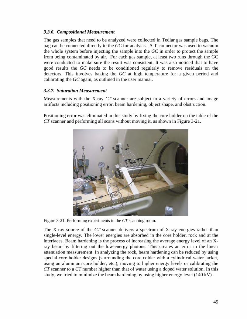
45

3.3.6. Compositional Measurement

The gas samples that need to be analyzed were collected in Tedlar gas sample bags. The bag can be connected directly to the GC for analysis. A T-connector was used to vacuum the whole system before injecting the sample into the GC in order to protect the sample from being contaminated by air. For each gas sample, at least two runs through the GC were conducted to make sure the result was consistent. It was also noticed that to have good results the GC needs to be conditioned regularly to remove residuals on the detectors. This involves baking the GC at high temperature for a given period and calibrating the GC again, as outlined in the user manual.

3.3.7. Saturation Measurement

Measurements with the X-ray CT scanner are subject to a variety of errors and image artifacts including positioning error, beam hardening, object shape, and obstruction.

Positioning error was eliminated in this study by fixing the core holder on the table of the CT scanner and performing all scans without moving it, as shown in Figure 3-21.

Figure 3-21: Performing experiments in the CT scanning room.

The X-ray source of the CT scanner delivers a spectrum of X-ray energies rather than single-level energy. The lower energies are absorbed in the core holder, rock and at the interfaces. Beam hardening is the process of increasing the average energy level of an X-ray beam by filtering out the low-energy photons. This creates an error in the linear attenuation measurement. In analyzing the rock, beam hardening can be reduced by using special core holder designs (surrounding the core colder with a cylindrical water jacket, using an aluminum core holder, etc.), moving to higher energy levels or calibrating the CT scanner to a CT number higher than that of water using a doped water solution. In this study, we tried to minimize the beam hardening by using higher energy level (140 kV).

46

The X-shaped artifacts created by the object shape are eliminated by the cylindrical design of the core holder which has the same circular cross-sectional shape as expected by the CT inversion algorithms (which are designed for the human body).

The scanning slices were chosen carefully to be located between the sample ports. The tubing and plastic valve handles were removed to make sure the scanning slices were clear of any obstruction to achieve the best result possible (Figure 3-22 and Table 3-3). Slice #1 is on the upstream of P1, slice #2 is between P1 and P2, etc., and slices #7 and #8 are on the downstream of P7.

Figure 3-22: Core holder’s setting up for CT scanning.

Table 3-3: Scanning positions

Slice Distance from the upstream edge of the

core holder (mm)

Thickness of the slice

(mm)

1 118 3

2 158 3

3 198 3

4 238 3

5 278 3

6 318 3

7 358 3

8 370 3

47

In order to calculate the saturation at experimental conditions, we need CTgr, CTcr, CTexp. CTgr, CTcr to be measured at a pressure of about 1,600 psi which is close to the average pressure along the core during the experiment. To saturate the core with liquid n-butane at 1,600 psi, liquid n-butane was first transferred to an empty piston cylinder then nitrogen was used to push on the back of the piston. After being saturated with methane or liquid n-butane at 1,600 psi, the core was left for 30 minutes to make sure all pores were filled.

49

Chapter 4

4. Results and Discussions

4.1. Absolute Permeability Measurement

y = 13.921x + 9.3668R2 = 0.9759

0

2

4

6

8

10

12

14

16

0 0.05 0.1 0.15 0.2 0.25 0.3 0.35

1/Pm (atm)

k (m

d) Measure pointsLinear (Measure points)

Figure 4-1: Absolute permeability measurement using nitrogen

Figure 4-1 shows a plot of nitrogen permeability versus 1/pm. The liquid permeability is

the value of the intercept with the vertical axis, or 9.3 md in this case.

4.2. Porosity Measurement

Using the material balance method, the porosity of the core was measured to be around 16%.

4.3. Composition

4.3.1. Gas-Condensate Core Flooding Experiments

Noncapture Experiments

The compositional distribution along the core during a gas-condensate noncapture experiment is shown in Figure 4-2. No-flow samples were taken before the flow test when the gas mixture was above the dew-point. The no-flow compositions were repeated perfectly and were identical to the composition from the source cylinder. This

50

confirmation indicated that the rock does not have an effect on the (static) phase behavior of the gas mixture.

During flow through the core, going from left to right, the pressure drop was higher. Liquid dropped out in the core and accumulated in the rock. The flowing mixture became lighter (more C1) and the concentration of nC4 in the flowing phase along the core decreased.

0

2

4

6

8

10

12

14

16

18

20

0 1 2 3 4 5 6 7 8

Port

n-C

4(%

)

Noflow batch 1

Flow ing batch

Cylinder

Noflow batch 2

Flow direction

Figure 4-2: Gas-condensate noncapture experiment 1: nC4 in the flowing mixture.

Figure 4-3 and Figure 4-4 show two more noncapture experiments following the same procedure. The compositional distributions along the core confirm the result in Figure 4-2. These results also confirm the three region theory shown earlier in Figure 2-11 and the simulations results in Figure 3-6.

51

0

2

4

6

8

10

12

14

16

18

20

0 1 2 3 4 5 6 7 8

Port

n-C

4(%

)

Noflow batch 1

Flow ing batch

Cylinder

Noflow batch 2

Flow direction

Figure 4-3: Gas-condensate noncapture experiment 2: nC4 in the flowing mixture.

0

2

4

6

8

10

12

14

16

18

20

0 1 2 3 4 5 6 7 8

Port

n-C

4(%

)

Noflow batch 1

Flow ing batch

Cylinder

Noflow batch 2

Flow direction

Figure 4-4: Gas-condensate noncapture experiment 3: nC4 in the flowing mixture.

52

The effect of producing pressure (BHP in a real well) on the composition is shown in Figure 4-5. The result in Figure 4-5 shows that the higher the pressure drop below the dew-point the more nC4 accumulates in the condensate, and the less nC4 is found in the flowing mixture. This result confirms the simulation result reported previously by Shi (2009). This finding is important because it tells us a way to minimize the condensate banking by minimizing the pressure drop below the dew-point by either producing the well at higher pressure or applying partial pressure maintenance using gas cycling for example.

0

5

10

15

20

25

30

0 1 2 3 4 5 6 7 8

Port

nC4(

%)

Noflow

Cylinder

Flow (dow nstream p =1500 psi)

Flow (dow nstream p =1000 psi)

Flow direction

Figure 4-5: Gas-condensate noncapture experiment: nC4 in the flowing mixture with different

BHP control cases.

The results of revaporization study are shown in Figure 4-6 to Figure 4-8. From these figures, we can see that after 35 minutes the condensate does not revaporize into gas. This confirms the shift of the phase envelope and hence that shutting the well is not a good strategy to remove the condensate bank.

53

0

5

10

15

20

25

30

0 1 2 3 4 5 6 7 8

Port

n-C

4(%

)

Noflow

Cylinder

35 mins after shut-in

Flow direction

Figure 4-6: Condensate revaporization after noncapture experiment for gas-condensate system 1.

0

5

10

15

20

25

30

0 1 2 3 4 5 6 7 8

Port

nC4(

%)

Noflow

Cylinder

Flow

40 mins after shut-in

Flow direction

Figure 4-7: Condensate revaporization after noncapture experiment for gas-condensate system 2.

54

0

5

10

15

20

25

30

0 1 2 3 4 5 6 7 8

Port

nC4(

%)

Noflow

Cylinder

Flow

40 mins after shut-in

Flow direction

Figure 4-8: Condensate revaporization after noncapture experiment for gas-condensate system 3.

Capture Experiments

The results of a capture experiment are shown in Figure 4-9. Good repeatability was achieved under both static conditions and flowing conditions. The compositional distribution along the core shows a similar trend of liquid dropout as the trend seen during noncapture experiments. A second capture experiment also confirmed the result (Figure 4-10).

0

2

4

6

8

10

12

14

16

18

20

0 1 2 3 4 5 6 7 8

Port

n-C

4(%

)

Noflow batch 1

Flow ing batch 1

Cylinder

Noflow batch 2

Flow ing batch 2

Flow direction

Figure 4-9: Gas-condensate capture experiment 1.

55

0

2

4

6

8

10

12

14

16

18

20

0 1 2 3 4 5 6 7 8

Port

n-C

4(%

)

Noflow batch 1

Flow ing batch 1

Cylinder

Noflow batch 2

Flow ing batch 2

Flow direction

Figure 4-10: Gas-condensate capture experiment 2.

Figure 4-11 shows the result of another capture experiment. However in this case, after taking samples in the capture mode, we discharged all gas and condensate into a vacuumed empty cylinder. When the core and discharge cylinder reached pressure equilibrium (at low pressure), we disconnected the core from the cylinder and took samples from each of them. The nC4 compositions in the discharge cylinder and core were very high, which confirmed that the liquid condensate deposited in the core was rich in nC4.

0

10

20

30

40

50

60

70

80

90

100

0 1 2 3 4 5 6 7 8

Port

n-C

4(%

)

Noflow

Cylinder

Flow ing

Cylinder_Discharge

Core_discharge

Flow direction

Figure 4-11: Gas-condensate capture experiment 3.

56

4.3.2. Gas-Condensate-immobile Water Core Flooding Experiments

Noncapture Experiments

Comparing Figures 4-2 to 4-8 (without water in the core) to Figures 4-12 and Figure 4-13 for the system with immobile water in the core, it is clear that in the presence of immobile water, condensate still dropped out in the core. The higher the pressure drop, the more liquid dropped out in the core and accumulated in the rock. The flowing mixture became lighter (more C1) and the concentration of nC4 in the flowing phase decreased.

0

2

4

6

8

10

12

14

16

18

20

0 1 2 3 4 5 6 7 8

Port

n-C

4(%

)

Noflow batch 1

Flow ing

Cylinder

Noflow batch 2

Flow direction

Figure 4-12: Gas-condensate-immobile water noncapture experiment 1: nC4 in the flowing

mixture.

57

0

2

4

6

8

10

12

14

16

18

20

0 1 2 3 4 5 6 7 8

Port

n-C

4(%

)

Noflow batch

Flow ing

Cylinder

Flow direction

Figure 4-13: Gas-condensate-immobile water noncapture experiment 2: nC4 in the flowing

mixture.

Capture Experiments

Again, water did not have any effect on the compositional variation (Figure 4-14 and Figure 4-15). Condensate drop-outs were the same as in the two-phase system in Figures 4-9 to 4-11. The nC4 compositions of the discharge cylinder sample and core samples also increased, which further confirmed the accumulation of nC4 in the condensate that had dropped out in the core.

58

0

10

20

30

40

50

60

70

80

90

100

0 1 2 3 4 5 6 7 8

Port

n-C

4(%

)

Noflow

Cylinder

Flow ing

Cylinder_discharge

Core_discharge

Flow direction

Figure 4-14: Gas-condensate-immobile water capture experiment 1.

0

10

20

30

40

50

60

70

80

90

100

0 1 2 3 4 5 6 7 8

Port

n-C

4(%

)

Noflow

Cylinder

Flow ing

Cylinder_discharge

Core_discharge

Flow direction

Figure 4-15: Gas-condensate-immobile water capture experiment 2.

4.4. Saturation

Figures 4-16 shows condensate saturation distribution calculated from CT scanning. Slice #1 is on the upstream of P2, slice #2 is between P1 and P2, etc., and slices #7 and #8 are on the downstream of P7. The condensate saturation profile is consistent with the nC4 compositional profile, even though the saturation value estimated at slice #8 is suspect. It should be noted that due to the low porosity rock, there is only a small density difference between the liquid n-butane and methane, so the difference between CT numbers of C1-nC4 mixture saturated, C1-saturated and nC4-saturated rock is not large. This limits the accuracy of the saturation estimation. Besides that, the titanium core holder caused beam hardening which reduces the signal to noise ratio and increased the measurement error.

59

Figure 4-17 shows scanning of the titanium core holder with only air and water inside (no core). Due to the beam hardening, the CT values of air and water inside the titanium core holder were falsely measured as -625 H and 837 H respectively whereas the correct values are -1000 H and 0 H respectively. Figure 4-18 shows CT scanning of air and water inside an aluminum tube. The CT number of air and water inside the aluminum tube were -965 H and -1 HA respectively which are very close to the correct values. Hence a high pressure aluminum core holder would be better than titanium for CT scanning as the aluminum is more transparent to the X-rays.

0

2

4

6

8

10

12

14

16

18

20

0 1 2 3 4 5 6 7 8

Port

n-C

4(%

)

Flow ing batch

Cylinder

Flow direction

(a)

0

10

20

30

40

50

60

70

80

90

100

0 1 2 3 4 5 6 7 8

Slice

Sc(%

)

Flow direction

(b)

Figure 4-16: Gas-condensate noncapture experiment 3: (a) nC4 in the flowing phases. (b) condensate saturation profile.

60

(a)

(b)

Figure 4-17: CT scanning of the empty titanium core holder: (a) with air inside. (n) with a water bottle inside.

61

(a)

(b)

Figure 4-18: CT scanning of an aluminum tube: (a) with air inside. (b) with a water bottle inside.

62

Chapter 5

5. Conclusion

5.1. General Conclusions

The main conclusions of this study are:

• Repeatability of the capture and noncapture experiments was achieved, demonstrating the validity of the results.

• Due to the relative permeability and the consequent difference in mobilities of gas and condensate phase, the local composition will change hence the phase envelope of the mixture will shift.

• Condensate banking still occurs in the presence of immobile water. Water did not have any measurable effect on the compositional variation of the gas condensate in the experiments done here.

• Shutting a well to remove the condensate banking is not a good strategy as the condensate will not be able to revaporize due to the shift of the phase envelope.

• Condensate banking can be reduced by minimizing the pressure drop below the dew-point, either by producing the well slowly or by applying partial pressure maintenance using gas injection.

5.2. Suggestions for Future Work

First, as we can see from saturation results in Section 4.4, the titanium core holder attenuated the X-rays during CT scanner. Future experiments should calibrate the scans to determine whether the range of CT value between all liquid and all gas is linear. Alternatively, an aluminum core holder may be more suitable.

Second, the Joule-Thompson effect, which can make the pressure depletion no longer isothermal should be considered as well.

Third, the question of how to produce a gas-condensate well to have the maximum production should be studied.

Finally, as a means of enhancing condensate recovery in the field the gas cycling method has been used, so the efficiency of this method should be quantified. Furthermore, the study can be extended to reservoir optimization using gas cycling.

63

Nomenclature

BHP = well flowing bottom-hole pressure. pd = dew-point pressure. C1 = methane. C4 = butane. nC4 = n-butane (normal butane). N2 = nitrogen. CO2 = carbon dioxide. C7+ = heptanes plus. CCE = Constant Composition Expansion. CVD = Constant Volume Depletion. PVT = Pressure Temperature Volume. Tc = critical temperature. pc = critical pressure. C5 = pentane. Swi = immobile water saturation. CT = Computerized Tomography. CTA = CT number of the object “A”. µA = linear attenuation coefficient of object “A". Sc = condensate saturation. CTgr = CT number of gas saturated rock. CTcr = CT number of condensate saturated rock. CTexp = CT number of rock during experiments with C1-nC4 mixture. P2 = port #2. GC = Gas Chromatography. TCD = thermal conductivity detector. PLOT = Porous Layer Open Tubular. DI = Deionized. kg = gas permeability. pin = inlet pressure. pout = outlet pressure. Qout = volumetric flowrate measured at the outlet.

64

L = length of a core. A = cross-sectional area of a core.

65

References

Afidick, D., Kaczorowski, N.J., and Bette, S., 1994, “Production Performance of a Retrograde Gas Reservoir: A Case Study of the Arun Field”, Presentation at SPE Asia Pacific Oil and Gas Conference, Melbourne, Australia, SPE 28749.

Agilent Technologies, 2008, “Agilent 3000 Micro Gas Chromatograph”, User Information, Third Edition.

Agilent Technologies, “Agilent Cerity Tutorial”. Akin, S. and Kovscek, A.R., 2003, “Computed Tomography in Petroleum

Engineering Research”. Geological Society special publications, pp 22–38. Ali, J.K., McGauley, P.J., and Wilson, C.J., 1997, “Experimental Studies and

Modeling of Gas Condensate Flow near the Wellbore”, Presentation at Fifth Latin America and Caribbean Petroleum Engineering Conference and Exhibition, Brazil, SPE 39053.

Allen F.H. and Roe R. P., 1950, “Performance Characteristics of a Volumetric Condensate Reservoir”, Petroleum Transaction, AIME, Vol. 189.

Aziz, K., Durlofsky, L., and Tchelepi, H., Winter 2010, “Notes for ENERGY 223: Reservoir Simulation”, Stanford University.

Aziz, R.M., 1985, “Deliverability Projection Model for Overpressure Gas-Condensate Reservoirs”, SPE Middle East Oil Technical Conference and Exhibition, Bahrain, SPE 13706.

Barnum, R.S., Brinkman, F.P., Richardson, T.W., and Spillette, A.G., 1995, “Gas Condensate Reservoir Behavior: Productivity and Recovery Reduction Due to Condensation”, Presentation at SPE Annual Technical Conference and Exhibition, Dallas, USA, SPE 30767.

Bengherbia, M. and Tiab, D., 2002, “Gas-Condensate Well Performance Using Compositional Simulator: A Case Study”, Presentation at SPE Gas Technology Symposium, SPE 75531.

Chunmei, S., 2009, “Flow Behaviors of Gas Condensate Wells”, Ph.D. Dissertation, Stanford University, California.

Coats, K. H. and Thomas, L.K., 1998, “Compositional and Black Oil Reservoir Simulation”, SPE Reservoir Evaluation & Engineering, August 1998.

Coats, K. H., 1980, “An Equation of State Compositional Model”, SPEJ, Oct 1980. Coats, K. H., 1985, “Simulation of Gas Condensate Reservoir Performance”, JPT. Danesh, A., 1998, “PVT and Phase Behaviour of Petroleum Reservoir Fluids”,

Elsevier Science B.V.

66

Economides, M.J., Dehghani, K., Ogbe, D.O., and Ostermann, R.D., 1987, “Hysteresis Effects of Gas Condensate Wells Undergoing Buildup Tests below the Dew Point Pressure”, Presentation at SPE Annual Technical Conference and Exhibition, Dallas, USA, SPE 16748.

Eilerts, C.K., Sumner E.F and Potts N.L., 1965, “Integration of Partial Differential Equation for Transient Radial Flow of Gas-Condensate Fluids in Porous Structures”, SPEJ 141.

El-Banbi, A.H and McCain W.D., 2000, “Investigation of Well Productivity in Gas-Condensate Reservoirs”, Presentation at SPE/CERI gas Technology Symposium, Calgary, Canada, SPE 59773.

Fevang, Φ, 1995, “Gas Condensate Flow Behavior and Sampling”, Ph. D. Dissertation, University of Trondheim.

Fevang, Φ and Whitson, C.H., 1996, “Modeling Gas-Condensate Well Deliverability”, SPE Reservoir Engineering, pp 221-230.

Fussel, D.D., 1973, “Single-Well Performance Predictions for Gas Condensate Reservoirs”, JPT 258, Trans. , AIME, 255.

GE Medical System, 2000, “HiSpeed CT/i Technical Reference Manual”, Rev 8. GE Medical System, “HiSpeed CT/i TiP Tutorial”, Rev. 4, A Training in Partnership

Program. Gerritsen, M., 2008, “Fundamental of Petroleum Engineering”, E120 lecture slides. Hagoort, J., 1988, “Fundamentasl of Gas Reservoir Engineering”, Elsevier Science

B.V. Ikoku, C.U., 1984, “Natural Gas Reservoir Engineering”, John Wiley & Sons Inc. Jones, J.R. and Raghavan, R., 1985, “Interpretation of Flowing Well Responses in

Gas – Condensate Wells”, Presentation at SPE Annual Technical Conference and Exhibition, Las Vegas , Nevada, SPE 14204.

Jones, J.R., Vo, D.T., and Raghavan, R., 1986, “Interpretation of Pressure Buildup Responses in Gas – Condensate Wells”, Presentation at SPE Annual Technical Conference and Exhibition, New Orleans, SPE 15535.

Kay, W. B., 1940, “Pressure-Volume-Temperature Relations for n-Butane”, Ind. Eng. Chem., 32 (3), pp 358–360.

Kniazeff, V.J. and Naville, S.A., 1965, “Two-Phase Flow of Volatile Hydrocarbons”, SPEJ 37, Trans., AIME, 234.

Kovscek, A. R., Autumn 2010, “Petroleum Hydrocarbon Thermodynamics: An Equation of State Approach”, Stanford University.

Lal, R.R., 2003, “Well Testing in Gas-Condensate Reservoir”, M.Sc. Thesis, Stanford University.

McCain, W.D.Jr., 1990, “The Properties of Petroleum Fluids”, Second edition, PennWell Books.

McCain, W.D.Jr., Bridges, B., 1994, “Heavy Components Control Reservoir Fluid Behavior”, JPT, Sep. 1994.

67

McCain, W.D.Jr., 1994, “Volatile Oils and Retrograde Gases – What’s the difference?”, Petroleum Engineering International 35.

Muscat, M., 1949, “Physical Principles of Oil Production”, McGraw-Hill Book Company, Inc.

Nikravesh, M. and Soroush, M., 1996, “Theoretical Methodology for Prediction of Gas-Condensate Flow Behavior”, Presentation at SPE Annual Technical Conference and Exhibition, Denver, USA, SPE 36704.

Novosad, Z., 1996, “Compositional and Phase Changes in Testing and Producing Retrograde Gas Wells”, SPE Reservoir Engineering, November 1996.

O’Dell, H.G. and Miller, R.N., 1967, “Successfully Cycling a Low Permeability, High-Yield Gas-Condensate Reservoir”, JPT 41, Trans., AIME, 240.

Pedersen, K.S., Fredenslund, Aa., and Thomassen, P., 1989, “Properties of Oils and Natural Gases”, Gulf Publishing Company.

Perry, A.J, 1981, “Introduction to Analytical Gas Chromatography”, Marcel Dekker, Inc.

Roebuck, I.F., Henderson, G.E., Doughlas, J., Ford, W.T., 1968, “The Compositional Reservoir Simulator: Case I –The Linear Model”, SPEJ March, 1969 115-130.

Roebuck, I.F., Ford, W.T., Henderson, G.E., Doughlas, J., 1968, “The Compositional Reservoir Simulator; Case IV – The Two Dimensional Model”, SPE Annual Meeting, Houston, Texas, SPE 2235.

Roussennac, B., 2001, “Gas Condensate Well Testing Analysis”, M.Sc. Thesis, Stanford University, California.

Saeidi, A. and Handy, L.L., 1974, “Flow and Phase Behavior of Gas Condensate and Volatile Oils in Porous Media”, SPE Annual California Regional Meeting, SPE 4891.

Salam, E.A., Mucharam, L., Abdassah, D., Parhusip, B., and Panjaitan, P.R., 1996, “Modification of the CVD Test Approach and Its Application for Predicting Gas Deliverability from Gas-Condensate Reservoir of Talang Akar Formation in Indonesia”, Presentation at SPE Gas Technology Conference, Calgary, Canada, SPE 35648.

Scott, R. P.W., 1998, “Introduction to Analytical Gas Chromatography”, Chromatographic Sciences Series, Volumes 76.

Seminar papers from two conferences held, “North Sea Gas Condensate Reservoir & Their Development 1982”, May & October 1982, published by Oyez Scientific & Technical Services Ltd.

Shen, P., Luo, K., Zheng, X., Li, S., Dai, Z., and Liu, H., 2001, “Experimental Study of Near-Critical Behavior of Gas Condensate Systems”, Presentation at SPE Production and Operation Symposium, Oklahoma, USA, SPE 67285.

Sigmund P.M., Dranchuk, P.M., Morrow, N.R., and Purvis, R.A., 1971, “Retrograde Condensation in Porous Media’’, Presentation at SPE Annual Fall Meeting, New Orleans, SPE 3476.

68

Standing, M.B., 1952, “Volumetric and Phase Behavior of Oilfield Hydrocarbon Systems”, Reinhold Publishing Corporation.

Vinegar, H. and Wellington, S., 1987, “Tomographic imaging of three-phase flow experiments”. Rev. Sci. Instrum. 58 January 1987.

Vinegar, H. and Wellington, S., 1987, “X-Ray Computerized Tomography”, Journal of Petroleum Technology, August 1987.

Whitson, C. H. and Brulé, M. R., 2000, “Phase Behavior”, SPE monograph, volume 20.

Zhang, H.R. and Wheaton, R.J., 2000, “Condensate Banking Dynamics in Gas Condensate Fields: Compositional Changes and Condensate Accumulation around Production Wells”, Presentation at SPE Annual Technical Conference and Exhibition, SPE 62930.

69

Appendix A

A. Gas-condensate Simulation Input File

-- ECLIPSE INPUT FILE -- Production PERFORMANCE OF A L= 30 cm, D=5.06 cm Cylindrical core. -- Gas-condensate draw down test -- Permeability = 9 md, Porosity = 16.0% -- Modified 05/14/10 Add smooth krw functions -- Simulator: Eclipse 300, 2001 v -- The purpose is to design the Gas-condensate: -- determine the composition and liquid saturation -- distribution in the core. RUNSPEC ============================================================ OIL GAS FULLIMP WELLDIMS 10 50 3 3 5 10 5 4 3 0 / DIMENS 51 1 1 / NSTACK 50/ -- condensate ISGAS -- Units: LAB -- Number of components: implies compositional run COMPS 2 / MISCIBLE / FMTOUT UNIFOUT

70

GRID ============================================================ -- PV = 0.3*5000 m^2 INIT DX 51*0.51837 / DY 51*4.48 / DZ 51*4.48 / --OLDTRAN -- Porosity and permeability --- (Rock) BOX --- IX1-IX2 JY1-JY2 KZ1-KZ2 1 51 1 1 1 1 / INCLUDE 'Perm.txt'/ --- TOP Specification --BOX --- IX1-IX2 JY1-JY2 KZ1-KZ1 -- 1 1 1 1 1 1 / TOPS 51*0.0 / ENDBOX --- TOP Specification --BOX --- IX1-IX2 JY1-JY2 KZ1-KZ1 -- 1 1 1 1 1 1 / TOPS 51*1 / ENDBOX PROPS ============================================================ -- Properties section: PVT data from INCLUDE file EOS PR / -- Names of Components CNAMES C1

71

nC4 / -- Miscibility exponent MISCEXP 0.000000001 / -- Component Critical Temperatures (K) TCRIT 190.5611111 425.2 / -- Component Critical Pressures (atm) PCRIT 45.44 37.46953 / -- Component Critical Volumes (m3/kg-mole) -- set by user VCRIT 0.098 0.255 / -- Component acentric factor ACF 0.013 0.201 / -- Components Parachors (dyn/cm) -- (for IFT - Fanchi 1990) --PARACHOR --77 --189.9 / -- Peneleux Correction (Shift parameters DM-less) SSHIFT 0. 0. / -- Component Molecular Weight g/mol MW 16.04 58.12 / -- Binary interaction parameters BIC 0.0 /

72

STCOND 15.0 1.0 / -- Reservoir temperature: Deg C / K RTEMP --20 / 293.15K 20 / 293.15K -- Rock and fluid properties ROCK 132.7 0.00000000001 / --Gas saturation functions INCLUDE KrgoGC2.dat / MISCSTR -- miscibility surface tension reference 12.3048 / / STVP -- Surface tension with respect to pressure 300 12.3048 400 11.1124 500 9.9551 600 8.837 700 7.7623 800 6.7356 900 5.7616 1000 4.8454 1100 3.9918 1200 3.2063 1300 2.4941 1400 1.8605 1500 1.311 1600 0.8507 1700 0.4848 1800 0.2181 1850 0.1234 1900 0.0552 1925 0.0311 1950 0.0139 1975 0.0035 / / FVST --Specify miscibility variation with surface tension 0.0035 0.441977 0.0139 0.507334 0.0311 0.549881 0.0552 0.582353 0.1234 0.631138

73

0.2181 0.668126 0.4848 0.723684 0.8507 0.765544 1.311 0.799379 1.8605 0.827857 2.4941 0.852479 3.2063 0.874164 3.9918 0.893531 4.8454 0.911015 5.7616 0.92693 6.7356 0.941521 7.7623 0.954974 8.837 0.967438 9.9551 0.979032 11.1124 0.989859 12.3048 1.0 / / SOLUTION ============================================================ PRESSURE -- Pressure (atm) 51*149.7 / SGAS 1.0 50*1.0 / -- XMF -- 51*0.85 51*0.15 / XMF 51*0.00 51*0.00 / YMF 51*0.85 51*0.15 / -- Calculate initial oil and gas in place at surface conditions FIELDSEP 1 15.0 1.0 / / SUMMARY ============================================================ RUNSUM RPTONLY --Field Gas Production Rate WGPR PROD1 / / WGPT PROD1 / / WPIG

74

PROD1 / / WOPR PROD1 / / WOPT PROD1 / / WGOR PROD1 / / WBHP PROD1 / / WYMF PROD1 1 / / WYMF PROD1 2 / / WZMF PROD1 1 / / WZMF PROD1 2/ / --Producer block data BVOIL 50 1 1 / / --saturation and composition history for layer 4 INCLUDE 'BPRES.txt'/ INCLUDE 'BSOIL.txt'/ INCLUDE 'BXMF1.txt'/ INCLUDE 'BXMF2.txt'/ INCLUDE 'BYMF1.txt'/ INCLUDE 'BYMF2.txt'/ INCLUDE 'BBOIL.txt'/ INCLUDE

75

'BBGAS.txt'/ INCLUDE 'BMLSC2.txt'/ INCLUDE 'BMLST.txt'/ INCLUDE 'BVMF.txt'/ / SCHEDULE ============================================================ / WELLSPEC INJ1 G1 1 1 3* / PROD1 G2 51 1 3* / / WELLCOMP INJ1 1 1 1 1 1* 0.15875 5* / PROD1 51 1 1 1 1* 0.15875 5* / / -- Specify compositions of injection gas stream WELLSTRE LEANGAS 0.85 0.15 / / WCONINJE --INJ1 GAS AUTO BHP 125. / INJ1 GAS AUTO BHP 2* 149.7/ / WINJGAS INJ1 STREAM LEANGAS/ / WCONPROD PROD1 OPEN BHP 5* 68.72642 / --PROD1 OPEN BHP 2* 75./ / --RPTSCHED --PRESSURE SOIL KRG KRO / --PRESSURE SOIL XMF YMF ZMF VMF DENO DENG VOIL VGAS BOIL BGAS KRG KRO / --TSCRIT --0.00001 0.0000001 10 --/ TUNING

76

.000277 0.05 0.0000277 / / / TSTEP 60*0.00166667 60*0.5 / END

77

Appendix B

B. Gas-condensate with Immobile Water Simulation Input File

-- ECLIPSE INPUT FILE -- Production PERFORMANCE OF A Cylindrical core with dimesnsion L= 27.4 cm, D=5.06 cm . -- Gas-condensate draw down test -- Permeability = 2.1 mD, Porosity = 15.0% -- Modified from Shi's input file on 02/02/10 by adding water phase -- Simulator: Eclipse 300, 2001 v -- The purpose is to design the Gas-condensate experiment with the presence of immobile water: -- determine the length, permeability to get a suitable liquid saturation -- distribution in the core. RUNSPEC ============================================================ OIL GAS WATER FULLIMP WELLDIMS 10 50 3 3 5 10 5 4 3 0 / DIMENS 51 1 1 / NSTACK 50/ -- condensate ISGAS -- Units: LAB -- Number of components: implies compositional run COMPS 2 / MISCIBLE

78

/ FMTOUT UNIFOUT GRID ============================================================ -- PV = 0.3*5000 m^2 INIT DX 51*0.51837 / DY 51*4.48 / DZ 51*4.48 / --OLDTRAN -- Porosity and permeability --- (Rock) BOX --- IX1-IX2 JY1-JY2 KZ1-KZ2 1 51 1 1 1 1 / INCLUDE 'Physicalprop.txt'/ --- TOP Specification --BOX --- IX1-IX2 JY1-JY2 KZ1-KZ1 -- 1 1 1 1 1 1 / TOPS 51*0.0 / ENDBOX --- TOP Specification --BOX --- IX1-IX2 JY1-JY2 KZ1-KZ1 -- 1 1 1 1 1 1 / TOPS 51*1 / ENDBOX PROPS ============================================================ -- Properties section: PVT data from INCLUDE file EOS PR /

79

-- Names of Components CNAMES C1 nC4 / -- Miscibility exponent MISCEXP 0.000000001 / -- Component Critical Temperatures (K) TCRIT 190.5611111 425.2 / -- Component Critical Pressures (atm) PCRIT 45.44 37.46953 / -- Component Critical Volumes (m3/kg-mole) -- set by user VCRIT 0.098 0.255 / -- Component acentric factor ACF 0.013 0.201 / -- Components Parachors (dyn/cm) -- (for IFT - Fanchi 1990) --PARACHOR --77 --189.9 / -- Peneleux Correction (Shift parameters DM-less) SSHIFT 0. 0. / -- Component Molecular Weight g/mol MW 16.04 58.12 / -- Binary interaction parameters

80

BIC 0.0 / STCOND 15.0 1.0 / -- Reservoir temperature: Deg C / K RTEMP --20 / 293.15K 20 / 293.15K -- Rock and fluid properties ROCK 132.7 0.00000000001 / --Gas saturation functions INCLUDE kr3phase.txt / MISCSTR -- miscibility surface tension reference 12.3048 / / STVP -- Surface tension with respect to pressure 300 12.3048 400 11.1124 500 9.9551 600 8.837 700 7.7623 800 6.7356 900 5.7616 1000 4.8454 1100 3.9918 1200 3.2063 1300 2.4941 1400 1.8605 1500 1.311 1600 0.8507 1700 0.4848 1800 0.2181 1850 0.1234 1900 0.0552 1925 0.0311 1950 0.0139 1975 0.0035 / / FVST --Specify miscibility variation with surface tension 0.0035 0.441977 0.0139 0.507334

81

0.0311 0.549881 0.0552 0.582353 0.1234 0.631138 0.2181 0.668126 0.4848 0.723684 0.8507 0.765544 1.311 0.799379 1.8605 0.827857 2.4941 0.852479 3.2063 0.874164 3.9918 0.893531 4.8454 0.911015 5.7616 0.92693 6.7356 0.941521 7.7623 0.954974 8.837 0.967438 9.9551 0.979032 11.1124 0.989859 12.3048 1.0 / / SOLUTION ============================================================ PRESSURE -- Pressure (atm) 51*149.7 / SWAT 0.16 50*0.16 / SGAS 0.84 50*0.84 / XMF --51*0.85 51*0.15 / 51*0.00 51*0.00 / YMF 51*0.85 51*0.15 / -- Calculate initial oil and gas in place at surface conditions FIELDSEP 1 15.0 1.0 / / SUMMARY ============================================================ RUNSUM RPTONLY --Field Gas Production Rate WGPR PROD1 / / WGPT

82

PROD1 / / WPIG PROD1 / / WOPR PROD1 / / WOPT PROD1 / / WGOR PROD1 / / WBHP PROD1 / / WYMF PROD1 1 / / WYMF PROD1 2 / / WZMF PROD1 1 / / WZMF PROD1 2/ / --Producer block data BVOIL 50 1 1 / / --saturation and composition history INCLUDE 'BPRES.txt'/ INCLUDE 'BSOIL.txt'/ INCLUDE 'BSWAT.txt'/ INCLUDE 'BSGAS.txt'/ INCLUDE 'BXMF1.txt'/ INCLUDE 'BXMF2.txt'/ INCLUDE

83

'BYMF1.txt'/ INCLUDE 'BYMF2.txt'/ INCLUDE 'BBOIL.txt'/ INCLUDE 'BBGAS.txt'/ INCLUDE 'BMLSC2.txt'/ INCLUDE 'BMLST.txt'/ INCLUDE 'BVMF.txt'/ / SCHEDULE ============================================================ / WELLSPEC INJ1 G1 1 1 3* / PROD1 G2 50 1 3* / / WELLCOMP INJ1 1 1 1 1 1* 0.15875 5* / PROD1 51 1 1 1 1* 0.15875 5* / / -- Specify compositions of injection gas stream WELLSTRE LEANGAS 0.85 0.15 / / WCONINJE --INJ1 GAS AUTO BHP 125. / INJ1 GAS AUTO BHP 2* 149.7 / / WINJGAS INJ1 STREAM LEANGAS/ / WCONPROD PROD1 OPEN BHP 5* 68.72642 / --PROD1 OPEN BHP 2* 75./ /

84

--RPTSCHED --PRESSURE SOIL KRG KRO / --PRESSURE SOIL XMF YMF ZMF VMF DENO DENG VOIL VGAS BOIL BGAS KRG KRO / --TSCRIT --0.00001 0.0000001 10 --/ TUNING .000277 0.05 0.0000277 / / / TSTEP 60*0.00166667 60*0.5 / END