compositional and incremental modeling and analysis … · compositional and incremental modeling...
TRANSCRIPT

COMPOSITIONAL AND INCREMENTAL MODELING AND ANALYSIS FOR
HIGH-CONFIDENCE DISTRIBUTED EMBEDDED CONTROL SYSTEMS
By
JOSEPH E. PORTER
Dissertation
Submitted to the Faculty of the
Graduate School of Vanderbilt University
in partial fulfillment of the requirements
for the degree of
DOCTOR OF PHILOSOPHY
in
Electrical Engineering
May, 2011
Nashville, Tennessee
Approved:
Janos Sztipanovits
Gabor Karsai
Xenofon Koutsoukos
Aniruddha Gokhale
Mark Ellingham

DEDICATION
To God, the Father of us all, for helping me find insight to solve problems, for giving me courage
to face fears and difficulties, and for putting wonderful people all along this journey. To Jesus Christ,
the Son of God, for continuing to drive darkness from my life, replacing it with the light of peace,
truth, joy, and love.
To Rebekah, my dearest companion, for many years of sacrifice and patience. This would never
have happened without you. Thank you for never giving up on me. To my wonderful and patient
children, for their encouragement and prayers.
Finally to our parents, for many years of guidance and for their moral and financial support.
ii

ACKNOWLEDGEMENTS
Special thanks goes to my advisor, Professor Janos Sztipanovits, for his support and for his
patience and willingness to allow me to pursue this line of work. Further, I would like to thank all
of the researchers and students with whom I have worked during these past years. Thank you for
your encouragement, friendship, patience, and enjoyable times working together.
Portions of this work were sponsored by the Air Force Office of Scientific Research, USAF, under
grant/contract number FA9550-06-0312, and the National Science Foundation, under grant NSF-
CCF-0820088. The views and conclusions contained herein are those of the authors and should not
be interpreted as necessarily representing the official policies or endorsements, either expressed or
implied, of the Air Force Office of Scientific Research or the U.S. Government.
iii

TABLE OF CONTENTSPage
DEDICATION . . . . . . . . . . . . . . . . . . . . . . . . . . . . . . . . . . . . . . . . . . ii
ACKNOWLEDGEMENTS . . . . . . . . . . . . . . . . . . . . . . . . . . . . . . . . . . . . iii
LIST OF TABLES . . . . . . . . . . . . . . . . . . . . . . . . . . . . . . . . . . . . . . . . vi
LIST OF FIGURES . . . . . . . . . . . . . . . . . . . . . . . . . . . . . . . . . . . . . . . viii
I. PROBLEMS IN MODEL-BASED DESIGN AND ANALYSIS FOR HIGH-CONFIDENCEDISTRIBUTED EMBEDDED SYSTEMS . . . . . . . . . . . . . . . . . . . . . . . . 1
Problems . . . . . . . . . . . . . . . . . . . . . . . . . . . . . . . . . . . . . . . . . . 4Contributions . . . . . . . . . . . . . . . . . . . . . . . . . . . . . . . . . . . . . . . . 5Dissertation Organization . . . . . . . . . . . . . . . . . . . . . . . . . . . . . . . . . 6
II. RELATED WORK . . . . . . . . . . . . . . . . . . . . . . . . . . . . . . . . . . . . 7
Modeling Tools . . . . . . . . . . . . . . . . . . . . . . . . . . . . . . . . . . . . . . . 7Compositional and Incremental Methods . . . . . . . . . . . . . . . . . . . . . . . . 8
Incremental Scheduling Analysis . . . . . . . . . . . . . . . . . . . . . . . . . . . 9Incremental Deadlock Analysis . . . . . . . . . . . . . . . . . . . . . . . . . . . . 17Compositional Stability Analysis . . . . . . . . . . . . . . . . . . . . . . . . . . . 27
III. THE EMBEDDED SYSTEMS MODELING LANGUAGE (ESMOL) . . . . . . . . . . 35
Overview . . . . . . . . . . . . . . . . . . . . . . . . . . . . . . . . . . . . . . . . . . 36Design Challenges . . . . . . . . . . . . . . . . . . . . . . . . . . . . . . . . . . . 36Solutions . . . . . . . . . . . . . . . . . . . . . . . . . . . . . . . . . . . . . . . . 38
Tools and Techniques . . . . . . . . . . . . . . . . . . . . . . . . . . . . . . . . . . . 42ESMoL Language . . . . . . . . . . . . . . . . . . . . . . . . . . . . . . . . . . . . . 44ESMoL Tool Framework . . . . . . . . . . . . . . . . . . . . . . . . . . . . . . . . . . 55
Stage 1 Transformation . . . . . . . . . . . . . . . . . . . . . . . . . . . . . . . . 55Stage 2 Transformation . . . . . . . . . . . . . . . . . . . . . . . . . . . . . . . . 63
Synchronous Semantics . . . . . . . . . . . . . . . . . . . . . . . . . . . . . . . . . . 71Evaluation . . . . . . . . . . . . . . . . . . . . . . . . . . . . . . . . . . . . . . . . . 74
Communications Test . . . . . . . . . . . . . . . . . . . . . . . . . . . . . . . . . 77Quad Integrator Model . . . . . . . . . . . . . . . . . . . . . . . . . . . . . . . . 78Quadrotor Model . . . . . . . . . . . . . . . . . . . . . . . . . . . . . . . . . . . . 84
Lessons and Future Work . . . . . . . . . . . . . . . . . . . . . . . . . . . . . . . . . 85
IV. INCREMENTAL SYNTACTIC ANALYSIS FOR COMPOSITIONAL MODELS: AN-ALYZING CYCLES IN ESMOL . . . . . . . . . . . . . . . . . . . . . . . . . . . . . 89
Overview . . . . . . . . . . . . . . . . . . . . . . . . . . . . . . . . . . . . . . . . . . 89
iv

Syntactic Analysis Challenges . . . . . . . . . . . . . . . . . . . . . . . . . . . . . 89Solutions . . . . . . . . . . . . . . . . . . . . . . . . . . . . . . . . . . . . . . . . 89
Tools and Techniques . . . . . . . . . . . . . . . . . . . . . . . . . . . . . . . . . . . 91ESMoL Component Model . . . . . . . . . . . . . . . . . . . . . . . . . . . . . . 91Cycle Enumeration . . . . . . . . . . . . . . . . . . . . . . . . . . . . . . . . . . . 92Hierarchical Graphs . . . . . . . . . . . . . . . . . . . . . . . . . . . . . . . . . . 92
Incremental Cycle Analysis . . . . . . . . . . . . . . . . . . . . . . . . . . . . . . . . 93Formal Model . . . . . . . . . . . . . . . . . . . . . . . . . . . . . . . . . . . . . . 93Algorithm Description . . . . . . . . . . . . . . . . . . . . . . . . . . . . . . . . . 95ESMoL Mapping . . . . . . . . . . . . . . . . . . . . . . . . . . . . . . . . . . . . 96
Evaluation . . . . . . . . . . . . . . . . . . . . . . . . . . . . . . . . . . . . . . . . . 98Fixed-Wing Example . . . . . . . . . . . . . . . . . . . . . . . . . . . . . . . . . 98Analysis Results . . . . . . . . . . . . . . . . . . . . . . . . . . . . . . . . . . . . 99
Future Work . . . . . . . . . . . . . . . . . . . . . . . . . . . . . . . . . . . . . . . . 101
V. INCREMENTAL TASK GRAPH SCHEDULE CALCULATION . . . . . . . . . . . . 104
Overview . . . . . . . . . . . . . . . . . . . . . . . . . . . . . . . . . . . . . . . . . . 104Semantic Analysis Challenges . . . . . . . . . . . . . . . . . . . . . . . . . . . . . 104Solutions . . . . . . . . . . . . . . . . . . . . . . . . . . . . . . . . . . . . . . . . 105
Tools and Techniques . . . . . . . . . . . . . . . . . . . . . . . . . . . . . . . . . . . 105Task Graph Scheduling Abstractions . . . . . . . . . . . . . . . . . . . . . . . . . 105BSA Scheduling Algorithm . . . . . . . . . . . . . . . . . . . . . . . . . . . . . . 106
Incremental Schedule Analysis . . . . . . . . . . . . . . . . . . . . . . . . . . . . . . 109Concepts . . . . . . . . . . . . . . . . . . . . . . . . . . . . . . . . . . . . . . . . 110Algorithm Definition . . . . . . . . . . . . . . . . . . . . . . . . . . . . . . . . . . 111
Future Work . . . . . . . . . . . . . . . . . . . . . . . . . . . . . . . . . . . . . . . . 113
VI. CONCLUSIONS: WHAT HAVE WE LEARNED? . . . . . . . . . . . . . . . . . . . . 115
BIBLIOGRAPHY . . . . . . . . . . . . . . . . . . . . . . . . . . . . . . . . . . . . . . . . 116
v

LIST OF TABLESPage
1 Common real-time scheduling algorithms . . . . . . . . . . . . . . . . . . . . . . . . 112 Resource supply models and their parameters. . . . . . . . . . . . . . . . . . . . . . . 123 Quantities for the sector formula. . . . . . . . . . . . . . . . . . . . . . . . . . . . . . 31
4 Acquisition relation transformation details. . . . . . . . . . . . . . . . . . . . . . . . 565 Actuation relation transformation details. . . . . . . . . . . . . . . . . . . . . . . . . 596 Local (processor-local) data dependency relation. . . . . . . . . . . . . . . . . . . . . 607 Transmit relation transformation details. This represents the sender side of a remote
data transfer between components. . . . . . . . . . . . . . . . . . . . . . . . . . . . . 618 Receive relation transformation details. . . . . . . . . . . . . . . . . . . . . . . . . . 619 Scheduling spec for the Quadrotor example. . . . . . . . . . . . . . . . . . . . . . . . 6610 Stage 2 Interpreter Template for the Scheduling Specification . . . . . . . . . . . . . 6611 Generated code for the task wrappers and schedule structures of the Quadrotor model. 6912 Template for the virtual machine task wrapper code. The Stage 2 FRODO interpreter
invokes this template to create the wrapper code shown in Table 11. . . . . . . . . . 7013 Sector value comparisons for simulation and execution on the actual platform. . . . . 82
14 Cycle analysis comparisons for the fixed wing model. . . . . . . . . . . . . . . . . . . 100
15 Function and variable definitions. . . . . . . . . . . . . . . . . . . . . . . . . . . . . . 10716 Function and variable definitions for incremental BSA. . . . . . . . . . . . . . . . . . 114
vi

LIST OF FIGURESPage
1 Facets of model-based CPS design processes. Reconciling all of the details representedby these models is a significant challenge for design tools. Tools must also supportrealistic work flows for development teams. . . . . . . . . . . . . . . . . . . . . . . . 2
2 Worst-case analysis interval for determining the supply bound function of the periodicresource model Γ for k = 3. Figure reproduced from [1, Fig. 4.1]. . . . . . . . . . . 13
3 DSSF example graphs. Figs. from [2]. . . . . . . . . . . . . . . . . . . . . . . . . . . 264 Block diagram interconnection examples for conic system composition rules. . . . . . 305 Block diagram interconnection example for feedback structure. . . . . . . . . . . . . 32
6 Flow of ESMoL design models between design phases. . . . . . . . . . . . . . . . . . 407 Platforms. This metamodel describes a simple language for modeling the topology of
a time-triggered processing network. . . . . . . . . . . . . . . . . . . . . . . . . . . . 428 Basic architecture for the quadrotor control problem. . . . . . . . . . . . . . . . . . . 449 Quadrotor component types model from the SysTypes paradigm. . . . . . . . . . . . 4610 SystemTypes Metamodel. . . . . . . . . . . . . . . . . . . . . . . . . . . . . . . . . . 4711 Overall hardware layout for the quadrotor example. . . . . . . . . . . . . . . . . . . 4812 Quadrotor architecture model, Logical Architecture aspect. . . . . . . . . . . . . . . 5013 Triply-redundant quadrotor logical architecture. This is not part of the actual quadro-
tor model, and is only given for illustration. . . . . . . . . . . . . . . . . . . . . . . . 5114 Quadrotor architecture model, Deployment aspect. . . . . . . . . . . . . . . . . . . . 5115 Details from the deployment sublanguage. . . . . . . . . . . . . . . . . . . . . . . . . 5216 Quadrotor architecture model, Timing aspect. . . . . . . . . . . . . . . . . . . . . . . 5317 Details from timing sublanguage. . . . . . . . . . . . . . . . . . . . . . . . . . . . . . 5418 Stage 1 Transformation. . . . . . . . . . . . . . . . . . . . . . . . . . . . . . . . . . . 5619 Acquisition relation in ESMoL Abstract, representing the timed flow of data arriving
from the environment. . . . . . . . . . . . . . . . . . . . . . . . . . . . . . . . . . . . 5620 Actuation relation in ESMoL Abstract, representing the timed flow of data back into
the environment. . . . . . . . . . . . . . . . . . . . . . . . . . . . . . . . . . . . . . . 5921 Local dependency relation in ESMoL Abstract, representing data transfers between
components on the same processing node. . . . . . . . . . . . . . . . . . . . . . . . . 6022 Transmit and receive relations in ESMoL Abstract, representing the endpoints of data
transfers between nodes. . . . . . . . . . . . . . . . . . . . . . . . . . . . . . . . . . . 6123 Object diagram from part of the message structure example from Figs. 12 and 14. . 6224 Stage 2 Interpreter. . . . . . . . . . . . . . . . . . . . . . . . . . . . . . . . . . . . . . 6325 Integration of the scheduling model by round-trip structural transformation between
the language of the modeling tools and the analysis language. . . . . . . . . . . . . . 6426 Conceptual development flow supported by the tool chain. . . . . . . . . . . . . . . . 7427 Hardware in the Loop (HIL) evaluation configuration. . . . . . . . . . . . . . . . . . 7728 Communications test model. . . . . . . . . . . . . . . . . . . . . . . . . . . . . . . . . 7729 Communications test plant model using the Mathworks xPC Target. . . . . . . . . . 7830 Simulink model of a simplified version of the quadrotor architecture. . . . . . . . . . 79
vii

31 Simplified quadrotor plant dynamics. The signal lines leading off the picture are signaltaps used for online stability analysis. . . . . . . . . . . . . . . . . . . . . . . . . . . 79
32 Conceptual nested loop structure of the controller. . . . . . . . . . . . . . . . . . . . 8033 Sector analysis block (SectorSearch) connection around the position controller. . . . 8134 Sector value evolution over time for the quad integrator. . . . . . . . . . . . . . . . . 8235 Magnitude frequency responses for the quad integrator. . . . . . . . . . . . . . . . . 8336 Simulink model of the Starmac quadrotor helicopter. . . . . . . . . . . . . . . . . . . 8437 Detail of the Robostix block. . . . . . . . . . . . . . . . . . . . . . . . . . . . . . . . 8538 Detail of the inner loop block. . . . . . . . . . . . . . . . . . . . . . . . . . . . . . . . 8639 Schedule configuration for the quadrotor. . . . . . . . . . . . . . . . . . . . . . . . . 8740 Timing diagram for the Robostix AVR running the inner loop controller. . . . . . . . 8741 Trajectory tracking for the quadrotor implementation. . . . . . . . . . . . . . . . . . 88
42 Simulink Fixed Wing Controller Model . . . . . . . . . . . . . . . . . . . . . . . . . . 9843 Synchronous data flow for Fixed Wing Controller . . . . . . . . . . . . . . . . . . . . 9944 Detail of the components involved in the cycle found in the velocity controller. . . . 10145 Full cycle for the velocity controller. . . . . . . . . . . . . . . . . . . . . . . . . . . . 103
viii

CHAPTER I
PROBLEMS IN MODEL-BASED DESIGN AND ANALYSIS FOR
HIGH-CONFIDENCE DISTRIBUTED EMBEDDED SYSTEMS
High confidence embedded control system software designs often require formal analyses to ensure
design correctness. Detailed models of system behavior cover numerous design concerns, such as
controller stability, timing requirements, fault tolerance, and deadlock freedom. Models for each
of these domains must together provide a consistent and faithful representation of the potential
problems an operational system would face. This poses challenges for structural representation of
models that can integrate software design details between components and across design domains,
as commonly components and design aspects are tightly coupled.
Coupling between separately designed components and modules can prevent model analyses from
scaling well to large designs. Coupling also occurs within individual systems and components between
behaviors represented by different design concerns (as represented by the layers shown in Fig. 1) as
different aspects of the design constrain design structures and parameters in different ways. These
complications combine with other factors to increase the difficulty of system integration. Integration
difficulties are well-documented for embedded systems [3], and for software projects in general [4].
As a simple example from the distributed embedded control systems domain, schedulability,
deadlock-freedom, and stability are three different notions of correctness that must be satisfied for
virtually any distributed real-time control system design. All three of these conditions can depend on
the frequencies at which real-time tasks are run, but each design concern constrains the frequencies
in a different way. For example, increasing sampling frequency can increase the stability of a control
loop, but which could make scheduling requirements difficult or impossible to satisfy. Extending
the same example, specifying additional timing constraints and dependencies between tasks in a
real-time system may improve end-to-end latency, but increase the risk of deadlock. We call this
interaction of constraints between disparate design concerns vertical coupling.
1

Figure 1: Facets of model-based CPS design processes. Reconciling all of the details represented bythese models is a significant challenge for design tools. Tools must also support realistic work flowsfor development teams.
A typical example of horizontal coupling (i.e. between components in a design, and within a
single design concern) is the problem of end-to-end latency requirements. The latency incurred
between a change in the physical environment and the control system’s response to that change
is often a critical matter. Numerous sensing, computation, data communication, and actuation
elements may lie on a timing-critical data dependency path between the initial sensing event and
the final actuation event. These elements usually share the same computing and communication
resources, so tightening one latency requirement to meet performance goals can easily render other
seemingly unrelated requirements infeasible. Often horizontal coupling is implicit – we usually
specify component parameters separately, resulting in adverse performance changes at the system
level due to unanticipated coupling.
2

Our solutions to the larger coupling problems in high-confidence embedded systems design revolve
around three main techniques:
1. Model-based design and analysis: Model-integrated computing [5] and related approaches
can prevent numerous structural and conceptual errors by encoding correctness concepts into
Domain-Specific Modeling Languages (DSMLs) used for design, and by resolving and encoding
relationships between details in different design aspects as language structures and constraints.
Inasmuch as system behaviors and behavioral notions of correctness can be encoded in a
modeling language and efficiently analyzed, these notions of correctness can be addressed by
the structure of design models [6].
2. Vertical decoupling: Several research efforts consider the problem of decoupling between
design domains – within a design we want to increase behavioral independence of elements of
the system with respect to a particular property so that design elements in different aspects can
be specified more or less independently. Examples include the Time-Triggered architecture[7],
which decouples functional specifications from timing specifications by providing a set of pro-
tocols to guarantee timing determinism and fault tolerance – protecting requirements in both
design aspects. Synchronous execution models reduce deadlock-freedom and decidability of
correctness properties to constraints on the structure and parameters of the design[8, 9]. Pas-
sive control theory guarantees stability of control loops through the proper interconnection
of passive components to maintain passivity at the system level [10, 11], and decreases the
destabilizing effects of sampling variance and time delays due to hardware [12, 13].
3. Horizontal decoupling: In model analysis we aim to exploit the structure of the model
to increase the scalability of analyses for that model. Two general techniques for addressing
scalability problems are compositional analysis and incremental analysis.
(a) Compositional analysis is a structural property of a formal analysis method (and com-
patible models) allowing the partition of a design into components. As analysis proceeds
we establish correctness properties first for the individual components and second for
the compositions of components using formal models of their interactions. Scalability
3

comes from successive analysis and combination of small component models, as opposed
to analyzing a single, large all-inclusive model.
(b) Incremental analysis relies on information stored in the model regarding previous analyses.
The idea is to isolate the effects of model changes (i.e. adding new components, removing
components, or modifying existing components) on the results of previous analyses. If
done efficiently, analysis must only be computed for components in the vicinity of the
changed components, where “vicinity” can be defined in a number of ways.
Cheaper analysis can yield significant cost reductions over the lifespan of a high-confidence control
software development project. Incremental analysis can further reduce costs by allowing rapid
redesigns when features are added to a deployed design.
Specific Problems
1. Continuous-time feedback control, embedded computer software, and distributed computing
hardware design domains are highly specialized and often conceptually incompatible. Sharing
model artifacts between designers in different domains can lead to inconsistency problems in
software implementations or other engineering artifacts due to incomplete or faulty under-
standing of design issues. These inconsistencies can seriously impact the soundness of model
analyses, and can hide design defects. Current state of the art resolves these problems by
reviewing many of the details in meetings and personal discussions. In the worst cases serious
incompatibilities are not discovered until very late in the development cycle, leading to project
overruns and cancellations.
2. Controller properties which are verified using simulation models may no longer be valid when
the design becomes software in a distributed processing network. Scheduling jitter, data com-
munication delays, and precision loss due to data quantization are all examples of effects that
contribute to instability and performance loss in controller software. Currently control design-
ers use conservative performance margins to avoid rework when performance is lost due to
deployment on a digital platform.
4

3. Long design, analysis, development, deployment, and test cycles limit the amount of iterative
rework that can be done to get a correct design. Currently high-confidence design requires both
long schedules and high costs. Lack of scalable formal model analysis methods is a significant
factor preventing rapid design evaluations.
4. Automating steps in different design and analysis domains for the same models and tools
requires a consistent view of inferred model relationships across multiple design domains. If
integrated tools have different views of the model semantics, then their analyses are not valid
when the results are integrated into the same design.
Contributions
In particular, we propose the following contributions toward solutions of the problems described
above:
1. Model Integration of High-Confidence Design Tools: We have created a DSML for
modeling and generating software implementations of distributed control systems, the Embed-
ded Systems Modeling Language (ESMoL). ESMoL includes aspects for functional modeling,
execution platforms, and mapping of functional blocks to execution platforms. The language
also includes appropriate parameters to capture timing behavior.
2. Extensible Language Interpreter Framework: We use a two-stage interpreter develop-
ment framework to isolate model interpreter code from the details of the front-end ESMoL
modeling language as we experiment with language design. The first stage transforms ESMoL
models to models in a language called ESMoL Abstract, resolving inferred model relations.
The second stage interpreters create analysis models, simulations, and platform-specific code.
We aim to give all of the model interpreters a single, consistent view of model details for
analysis and generation.
3. Integrated Incremental Cycle Analysis: The ESMoL tool suite includes an analyzer that
checks for delay-free loops in the assembled dataflow models.
5

4. Incremental Task Graph Schedule Calculation: We present a conceptual discussion of
an incremental method for calculating task graph schedules.
Dissertation Organization
• Chapter II discusses literature in the field that relates to our chosen solution methods.
• Chapter III discusses the design philosophy and key details of the ESMoL modeling language.
We include a discussion of an interpreter development architecture to improve the extensibility
and maintainability of the language and tools.
• Chapter IV gives an example of incremental syntactic analysis in ESMoL models.
• Chapter V covers incremental schedule calculation.
• Finally, chapter VI addresses lessons learned and potential future work in this area.
6

CHAPTER II
RELATED WORK
Modeling Languages and Tools for Embedded Systems Design
A number of projects seek to bring together tools and techniques which can automate different
aspects of high-confidence distributed control system design and analysis:
• AADL is a textual language and standard for specifying deployments of control system designs
in data networks[14]. AADL projects also include integration with the Cheddar scheduling
tool[15]. Cheddar is an extensible analysis framework which includes a number of classic
real-time scheduling algorithms[16].
• Giotto[17] is a modeling language for time-triggered tasks running on a single processor. Giotto
uses a simple greedy algorithm to compute schedules. The TDL (Timing Definition Language)
is a successor to Giotto, and extends the language and tools with the notion of modules
(software components)[18]. One version of a TDL scheduler determines acceptable communi-
cation windows in the schedule for all modes, and attempts to assign bus messages to those
windows[19].
• The Metropolis modeling framework[20] aims to give designers tools to create verifiable system
models. Metropolis integrates with SystemC, the SPIN model-checking tool, and other tools
for schedule and timing analysis.
• Topcased[21] is a large tool integration effort centering around UML software design languages
and integration of formal tools.
• Several independent efforts have used the synchronous language Lustre as a model translation
target (e.g. [22] and [23]) for deadlock and timing analysis.
7

• RTComposer[24] is a modeling, analysis, and runtime framework built on automata models. It
aims to provide compositional construction of schedulers subject to requirements specifications.
Requirements in RTComposer can be given as automata or temporal logic specifications.
• The DECOS toolchain [25] combines a number of existing modeling tools (e.g. the TTTech
tools, SCADE from Esterel Technologies, and others) but the hardware platform modeling and
analysis aspects are not covered.
We are creating a modeling language to experiment with design decoupling techniques, integra-
tion of heterogeneous tools, and rapid analysis and deployment. Many of the listed projects are too
large to allow experimentation with the toolchain structure, and standardization does not favor ex-
perimentation with syntax or semantics. Due to its experimental nature some parts of our language
and tool infrastructure change very frequently. As functionality expands we may seek integration
with existing tools or standards as appropriate.
Compositional and Incremental Methods
In order to introduce the topic, we will first use some definitions from Edwards et al [26] to clarify
terms and concepts in this research area. We have expanded the definitions and descriptions slightly
to better fit our approach.
A formal design consists of the following elements[26]:
• A specification of system functions and behavior, including any details necessary to determine
correctness with respect to requirements.
• A set of properties which the design must satisfy, that can be checked against the specification.
These are derived from requirements or are assumed for correct operation of any system (e.g.,
deadlock-freedom).
• A set of performance indices allowing us to assess the quality of a particular design.
• Constraints on the performance indices. These are also derived from requirements.
Edwards et al further classify properties as follows[26]:
8

1. Properties inherent to the model of computation (behavior), which can be shown to hold for
all specifications.
2. Syntactic properties can be determined by tractable analysis of the structure of elements in
the specification.
3. Semantic properties can only be determined by examining the actual behavior of the specifi-
cation. This means executing the specification either implicitly or explicitly over the full range
of inputs.
In our work we consider proper design specification and correctness properties, but have not
yet addressed performance indices and constraints beyond timing latency. In particular, we aim
to create modeling tools and techniques which favor correct design by constructing model-based
design environments that provide significant inherent properties for all well-formed models, or ef-
ficient analysis of syntactic properties. For semantic properties we seek abstractions which allow
us to encode correct behavioral relationships into the syntax of the specification language, reducing
expensive semantic analysis to less costly syntactic analysis.
We can now describe our approach to decoupling within this framework. We seek to achieve ver-
tical decoupling by selecting a platform (TTA) which provides timing determinism and synchrony
as inherent properties, and use passive control design methods to reduce the semantic property
of robust stability to a syntactic concern. For horizontal decoupling we aim to use compositional
techniques, which are inherently syntactic – for example, many properties in a design model can
be evaluated from the bottom-up, following the design hierarchy. We also use incremental meth-
ods to make evaluation of both syntactic and semantic properties more compatible with iterative
development processes.
Incremental Scheduling Analysis
Timing is a fundamentally semantic property. Determination of design validity and correctness de-
pend on properties only verifiable by execution of the behaviors of the model. In a design model we
can easily represent the relations between tasks, messages, and hardware for the purposes of syn-
thesizing simulations or even scheduling analysis problem specifications. However, these structures
9

have little bearing on determining the actual admissibility of tasks and messages into an existing
design. We can always draw the connections in the model, but only semantic analysis will yield an
indication of whether or not the model is well-formed with respect to schedulability, and whether it
satisfies latency constraints.
In most cases, useful compositional and incremental techniques for scheduling must introduce
some restriction of behavior or approximation into a problem which is highly coupled over the entire
system design in order to reduce that coupling for scalable analyses. As we will see in the sequel,
for some scheduling algorithms and correctness criteria, compositional and incremental analyses
can proceed without introducing approximations into the behaviors represented by the design. In
these cases the properties are specified locally (i.e. task deadlines), greatly limiting the effects of
dependencies but also greatly limiting the ability to express and enforce constraints which meet end-
to-end deadlines. The much more difficult and general case considers end-to-end latency over the
dependency graphs between tasks and messages. This forces us to properly model global coupling
in the design, but seriously complicates our efforts to find useful decoupling methods.
Hierarchical Schedulability Analysis Using Resource Interfaces
Hierarchical schedulability analysis is a technique for abstracting a set of hard real-time components
in such a way that multiple task sets could efficiently be composed and analyzed. More specifically,
1) we can analyze heterogeneous schedulability models, where different groups of tasks are run
together under different scheduling algorithms; and 2) given a working, feasible real-time system, we
can efficiently determine whether new task sets can be admitted for execution, even if they run under
different scheduling algorithms. Admission depends on safety and resource availability. Beyond the
compositional and incremental structure of models for analysis, hierarchical scheduling also requires
runtime scheduling algorithms that support hierarchical resource sharing.
We deal with computing tasks and data communication messages whose respective execution
times and data transfer times are known and bounded for the contention-free case. In this section
we will refer to all resource consumers (tasks and messages) as tasks for simplicity. We consider only
periodic tasks (or sporadic tasks with a known maximum frequency). A resource provides a known
10

Scheduling algorithm Priority scheme CompositionalityStatic schedule Fixed, non-preemptive Adding tasks incrementally requires
a priori restrictions (such asharmonic periods), or recomputationof the whole schedule.
EDF (Earliest Dynamic, preemptive Admitting new tasks is a function ofDeadline First) based on the next nearest utilization, which can be calculated
deadline to the current time. easily for the current workload.RM/DM (Rate Fixed, preemptive Admitting new tasks requires analysisor Deadline Priority determined against utilizations or demand bounds atMonotonic) by period or by all higher priority levels.
relative deadline.
Table 1: Common real-time scheduling algorithms
amount of capacity over time, and tasks consume that capacity when executing. Schedulability
implies that the resources supplied by scheduling algorithms are sufficient to meet the demand
imposed by the tasks.
Easwaran [27] clarifies two fundamental approaches to compositional scheduling analysis:
1. A task set may be considered abstractly as a single task demand function under a scheduling
algorithm which is global to all tasks. This approach was proposed by Wandeler [28]. Resources
are abstracted under a supply bound function (sbf), and tasks are composed under a demand
bound function (dbf) using the real-time calculus[29]. In this analysis approach the order in
which tasks are analyzed can affect the satisfaction of the schedulability property for fixed-
priority scheduling, so careful restrictions must be placed on the order of analysis.
2. A task set, its scheduling algorithm, and its resources can be seen as a new resource supply
function, which is the approach we will cover here. This technique has the advantage that
each component then presents a partial resource supply model to its child components, which
may also be composite. The resulting structure is a hierarchy of tasks, each with its own
resource supply function. During design and analysis, each set of supply-demand relationships
is restricted to its own scope in the model hierarchy. The hierarchical scheduling approach was
first proposed by Shin [1], and extended by Easwaran[27] to better model preemption overhead
and deadlines.
A runtime scheduling algorithm controls the execution of a task set to ensure that all tasks get
adequate resources. Scheduling algorithms are usually characterized by their priority policy. Table
11

Supply model Parameters Min sbf(t) CommentsBounded delay interval [t1, t2] c(t− δ) if t ≥ δ For any time interval
supply rate c 0 if t < δ [t1, t2], supplydelay bound δ c(t2 − t1) units
before time t2 + δ.Periodic period Π t− (k + 1)(Π−Θ) , Supply Θ units
supply Θ if t ∈ [(k + 1)Π− 2Θ, (k + 1)Π−Θ] every Π time units.(k − 1)Θ, if notk = max(d(t− (Π−Θ))/Πe , 1)
EDP (Explicit period Π⌊
t−(∆−Θ)Π
⌋Θ + max{0, Extends the periodic
Deadline supply Θ t− (Π + ∆− 2Θ)−⌊
t−(∆−Θ)Π
⌋Π} model with a deadline
Periodic) deadline ∆ if t ≥ ∆−Θ parameter ∆.0 otherwise
Table 2: Resource supply models and their parameters.
1 describes some common scheduling algorithms and their priority schemes, along with notes on the
details of incrementally extending models under each particular scheduling algorithm.
For supply models a constant supply is most common (i.e., s(t) = c), but other models have
better compositionality properties. Mok and Feng[30] introduced a bounded delay model for resource
supply. Shin and Lee[31][1] presented a model where a resource is modeled to provide a fixed amount
of supply at a constant periodic rate. Easwaran[27] extended the periodic supply model with support
for user-specified deadlines. The models and their parameters are described briefly in Table 2.
The key concept is that we can specify a real-time component as a collection of periodic tasks, a
scheduling algorithm, and a resource supply interface. The real-time component executes the tasks
according to the specified algorithm, subject to the supply constraints provided by the resource
model. This structure allows real-time components to be specified and executed as a hierarchy, as
each component’s resource interface appears as a single periodic task to the component at the next
higher level. The top level component provides the total (often constant) supply.
As an example we will describe the periodic supply model here in greater detail. A periodic
resource Γ supplies Θ units of resource every Π time units. The actual supply could occur anywhere
in each time interval of length Π, so we interpret the occurrence according to the worst case with
respect to schedulability: supply first occurs as early as possible where it might be missed for a
given analysis interval. In the worst case, the first supply is followed by a blackout interval of length
2(Π − Θ), followed by supply instances which occur as late as possible for all successive periods,
12

Figure 2: Worst-case analysis interval for determining the supply bound function of the periodicresource model Γ for k = 3. Figure reproduced from [1, Fig. 4.1].
sbfΓ(t) ={
t− (k + 1)(Π−Θ) if t ∈ [(k + 1)Π− 2Θ, (k + 1)Π−Θ](k − 1)Θ otherwise
(1)
k = max(d (t−(Π−Θ))
Π e, 1)
as shown in Fig. 2. In the figure t is the length of the analysis interval, starting at the point of
worst-case supply. The interval t starts with the blackout period 2(Π − Θ), marked by the dark
dashed arrows. During the blackout period the interface provides no supply. This figure shows an
analysis interval with three periods, and ending in the middle of a capacity interval.
Eq. 1 shows an expression for a supply bound function representing the worst-case supply for
a periodic resource interface as depicted in Fig. 2. For more tractable analysis, a linear supply
function is commonly used, as in Eq. 2.
Finally, we give the schedulability condition for fixed-priority systems as described in [1, Theorem
4.5.3]:
“A scheduling unit SU〈W,R, A〉 where W is a periodic [task] workload set, R is a periodic
resource Γ〈Π,Θ〉, and A is the RM scheduling algorithm, is schedulable (with worst-case resource
supply of R) iff
∀Ti ∈W, ∃ti ∈ [0, pi] dbfRM (W, ti, i) ≤ sbfΓ(ti)”.
”.
sbfΓ(t) ={
ΠΘ (t− 2(Θ−Π)) if t ≥ 2(Π−Θ)
0 otherwise(2)
13

The final relevant result we will discuss creates an periodic resource interface to model the
supply required by child tasks in a hierarchical scheduling model. This technique is only valid for
EDF scheduling, and includes preemption overhead.
[27, Def. 4.4] Multi-period composition For the child component Ci, let ki be the period at
which its interface provides resources. φki= 〈ki,Θki
〉 is the resource model in the interface ICi. For
parent component C and its operating period k, Θk can be found using the optimization problem
in Eq. 3.
minimize Θk
subject toΘk
k≥
n∑i=1
Θki
ki+ PO(ki)
2(k −Θk) ≤ mini=1...n{2(ki−Θki
−kiPO(ki))}2
(3)
Here PO(k) is the preemption overhead function, which bounds the demand contributed by
system overhead for a given interface period k. PO(ki) is then the overhead contributed by the
interface of component Ci due to the period mismatch between the resource interfaces for ICiand
IC . PO is given as a fraction of the period ki. One suggested form for the preemption overhead
function is PO(k) = Ak , where the constant A is specified by the designer from calibration data.
Multi-period composition for fixed-priority scheduling models and periodic resource interfaces is still
an open problem.
For dynamic scheduling, deadlines and dependencies complicate compositionality when consider-
ing end-to-end properties in a dataflow network. Adjusting the deadline of a single task can lead to
a loss of schedulability (or performance) for components in other parts of the system, affecting tasks
which may not have direct functional dependencies. Dependencies are implemented using offsets or
synchronization mechanisms in dynamic scheduling environments. Offset determination essentially
computes a static schedule for a subset of the tasks in the system to ensure they meet end-to-end
latency requirements. For explicit task synchronization, unbounded nesting of locks across differ-
ent priority levels can lead to undecidable response times for scheduling models. Platforms which
provide priority inheritance protocols can alleviate many situations arising from such task nesting
14

situations. The priority ceiling protocol explicitly limits the depth of chains of blocking calls between
processes at different priority levels, so response time bounds can always be calculated[32].
Incremental Techniques for System Designs
Static scheduling is generally not compositional. Kwok and Ahmad give a detailed survey and
evaluation of static task graph scheduling methods, including a discussion of the abstractions on
which those methods are based[33]. Schild and Wurtz [34] and Ekelin and Jonsson [35] describe
constraint models for static real-time scheduling problems, such as would be used in designs based
on time-triggered communication systems. Zheng and Chong give an alternate formulation of the
constraint models which is more complex, but allows the designer to optimize for extensibility[36].
The additional complexity is due to the addition of constraints and variables to model preemption
as well as the need to explicitly model task and message finish times in order to model slack. Using
preallocated slack to achieve incrementality is only a partial solution, as the technique only addresses
the availability of time to modify or change tasks and messages. It is a necessary condition, but not
sufficient. In order to have a sufficient condition we would also have to address changes or additions
to the data dependency graph.
For statically scheduled workloads Zheng and Chong give the following form (Eq. 4) for their
slack metrics[36]. Maximizing slack creates additional time in the schedule for modifying or adding
tasks and messages.
ME =∑
(ti,tj)∈ω
wti,tj × ((smti,tj− fti) + (stj − fm
ti,tj)) (4)
In Eq. 4 the set ω is the set of task instance pairs which have remote data dependencies. ti
is task instance i, stiis a variable representing its start time, and fti
is its end time. smti,tj
is the
start time of the message from task ti to task tj , and fmti,tj
is the corresponding end time. wti,tjis
a designer-specifiable optimization weight for each task pair in ω.
In Pop et al[37] the authors describe an incremental approach to the allocation, mapping, and
scheduling problems for a time-triggered platform with non-preemptive statically scheduled tasks
and TDMA communications. The task graph granularity of their models is very coarse, where a
15

vertex corresponds to an application, and edges correspond to dependencies from the perspective of
software maintenance. Two application vertices are dependent if modifying the first will also require
the modification of the second. Their approach relies on the specification of size and probability
parameters to control the provision and distribution of schedule slack in order to accommodate
future capacity. They assume a discrete set of possible task configurations, and then the designer
gives probability values to each element, based on the likelihood of needing to add something similar
to a future design. Their quality metrics are based on a cost function which combines slack size
and distribution. Bin packing is used to maximize the available slack, and a simulated annealing
approach is used to maximize the objective function.
Matic proposes an interface algebra which deals compositionally and incrementally with delay
and data dependencies given task arrival rates, latency bounds, task dependency graphs, and WCET
bounds. The algebraic formalism describes composition, interconnection, abstraction, and refine-
ment of components. Within these operations, the model structures jointly evaluate schedulability
(using the bounded-delay resource supply model of Mok and Feng[30]), causality, and end-to-end
delay[38]. The end-to-end delay bounds are specified cumulatively rather than globally, and the
author does not consider the conservatism of the formalism with respect to the behaviors that it
represents.
Ghosh et al present a formal model for allocation (Q-RAM) which searches over possible quality
levels (bandwidths), delay levels (hops), and routes for a set of communicating tasks[39]. The
immense size of the search space is pruned by considering the hierarchical structure of the network,
and exploiting locality of communication where possible. The objective is to flexibly, scalably, and
incrementally determine resource allocation on the network while maintaining near-optimality for a
utility metric. In [40] the authors present a distributed allocation scheme where each sub-domain
negotiates for a common global set point for its allocated tasks. Their approach is fundamentally
suited to incremental analysis, though their evaluations do not stress this aspect.
16

Incremental Deadlock Analysis
We consider compositional and incremental techniques related to deadlock detection or avoidance
in embedded system designs specified as dataflows. For many of these models deadlock-freedom is
an inherent property. Functional determinism is another important property inherent in dataflow
models of computation, but which we will not cover in detail. We shall rely on the fact that
synchronous data flows (SDF) exhibit both properties inherently. First, it will be important to
review some of the historical and current work in deadlock analysis.
Overview of Compositional Methods
Early work in semantics for distributed computing languages considered functional semantics – for
example, determining whether a given distributed dataflow network would deterministically calculate
a specified function [41]. Kahn showed that under proper assumptions, the network could calculate
the same function deterministically regardless of the firing order of the network. Kahn’s approach
used Scott continuity[42] to ensure the existence of a unique fixed point for the dataflow network. The
difficulty with this formalism is that while it provides compositional deadlock freedom, scheduling a
Kahn network is not compositional – although the data flow elements and their interconnections are
specified independently, scheduling or other analysis of the network may require global determination
of a fixed point (via iteration or symbolic analysis) in order to yield a result. Maximum capacities of
data buffers between components are also not decidable in the original Kahn formalism. Synchronous
data flow models of computation are a subset of the Kahn formalism for which the firing orders and
maximum buffer sizes can be precalculated [8] These data flow formalisms are compositional, and if
structured correctly can be used for incremental analysis.
SDF actors (functional components) are constrained to have fixed data token consumption and
production rates at each clock tick (firing). Balance equations on the topology of the data flow can
indicate whether the specified token flows are consistent, or whether each actor can be assigned a
specific number of firings to satisfy the rates in the specification [8]. For flow rate specifications, Buck
discusses the consequences of allowing richer data token flow models in the specification, such as
conditional execution and nondeterminism[9]. These constructs can easily lead to undecidability for
17

token flow rates on various data links and therefore lead to undecidability for maximum buffer sizes.
Lee and Parks illustrate that balance equations compose easily in hierarchical SDF specifications[43].
Balance equations may be given independently for subcomponents and solved to abstract the token
flow within the parent component to appear as a single actor having fixed token production and
consumption rates. For flow rates adding an actor or changing an existing actor may require firing
order sequence recomputation from the containing component to the top of the model hierarchy, so
the effects of incremental design changes on the analysis could be isolated.
As an example of the formalism, static scheduling of a SDF subsystem on a particular platform
means determining the firing order of all of the components, including the number of times each
component is fired. These values are determined using balance equations as described by Lee and
Messerschmitt[8]. In [8, Eq. 3] Lee gives a dynamic equation relating the amount of data in each of
the buffers to the firing sequence of the nodes and the topology of the SDF graph. We repeat some
of the discussion here to illustrate another fundamental model form for SDF analysis:
Let b[k] ∈ Zm represent the quantity of data in each of the buffers at discrete time tick k. Here
m is the number of edges in the SDF graph, associating one vector component with each buffer. Let
v[k] ∈ {0,1}n represent whether each node is fired at time k, where the components of the vector v
range over the nodes. Let the matrix Γ be defined as follows for the SDF graph:
Γi,j = token rate(nodej , edgei)
nodej is the jth node (component) in the graph, edgei is the ith edge (as in buffer vector b,
above), and token rate is the number of tokens produced on edgei by a single firing of nodej . For
nodes consuming data the value is negative. Then [8, Eq. 3] is given as
b[k + 1] = b[k] + Γv[k].
From the topology matrix Γ we can solve for the number of firings required to balance the SDF
graph or subsystem. If Γ has rank n− 1, then a positive integer vector q exists such that Γq = 0. q
represents the firing quantities. This is proved by Lee in [44].
18

More recently, Gossler and Sifakis proposed a formalism for modeling and analyzing asyn-
chronous designs based on a specification language known as BIP (for Behaviors, Interactions, and
Priorities)[45][46]. Component behaviors are modeled as automata, interactions as structures on
the sets of possible event combinations between connected components, and priorities are global
restrictions of the possible interactions. Bliudze and Sifakis give a formal definition for (possibly
asynchronous) event interactions represented by connectors in BIP[47]. These connectors can be
nested, and algebraic techniques are given for reducing hierarchical connectors to simpler represen-
tations. This provides the foundation for incremental design, as an existing (reduced) algebraic
model for the connectors in a design provides an interface for extending the design with additional
components and their interactions. New interactions can be “connected” to the existing connector
structure and analysis performed with respect to the reduced interaction model for those connec-
tors. Bensalem et al [48] give a detailed description of a formal model for incrementally constructing
the interaction space and efficiently computing behavior invariants for deadlock verification. These
techniques take a step towards reducing the semantic analysis required for deadlock analysis to a
syntactic analysis problem.
Ferrarini[49] deals with compositional design by giving the designer a safe set of building blocks
which allow the incremental construction of discrete control systems which satisfy boundedness,
cyclicness, and liveness. The analysis is reduced to a graph based on connections among tasks.
Synchronous Distributed Platforms
In standard real-time systems, distributed platforms typically do not provide fully synchronous se-
mantics. Synchronization between processes is provided by explicitly specified locking primitives
such as semaphores, mutexes, and monitors. Cyclic dependencies in these specifications can lead to
deadlock if they are not sequenced correctly. In addition, scheduling of tasks at different priorities
along with their dependencies can lead to deadlock or starvation (effective deadlock). For dynam-
ically scheduled tasks, the priority ceiling protocol can completely avoid priority-related deadlocks
by bounding the depth of chains of processes waiting on one another and by implicitly ordering the
acquisition and release of locks[32].
19

The Time-Triggered Architecture (TTA) relies on a priori knowledge of message schedules to
achieve and maintain synchronous execution over distributed processors. Each processor has a full
copy of the message schedule, and all messages are sent and received at precise, precalculated times.
Schedule-driven execution eliminates the need to send control and acknowledgment signals between
processing nodes, reducing horizontal coupling in the design.
The basic semantic assumptions of the TTA can be summarized as follows:
1. All clocks in the system are synchronized, and the schedules run over a global periodic cycle.
2. Data transfers occur on a common, shared bus where all messages are broadcast to all proces-
sors.
3. Data reading and writing are non-blocking for tasks.
4. Data message updates occur outside the execution window for sending/receiving tasks.
5. Messages on the bus do not preempt each other.
The Timed-Triggered Protocol (TTP) realizes the communication mechanism within the TTA.
Each processing node receives a TDMA time slot in which to send messages. TTP provides the
following services (see [50] for details):
• Timed message transport between nodes, reducing latency and jitter for individual transfers.
• Fault-tolerant distributed clock synchronization on all nodes, ensuring deterministic mode
change behavior for replicated computations.
• Fault-tolerant membership service for all nodes.
• Clique avoidance when faulty nodes are isolated from the network.
The Loosely Time-Triggered Architecture (LTTA) attempts to maintain the synchronous capa-
bilities of the TTA without the full clock synchronization between nodes, in order to reduce coupling
in the hardware architecture. LTTA is based on the following assumptions:
1. Assumption 1
20

• Each processing node has an independent local clock.
• Each shared variable (message) has a separate communication channel.
• Data reading and writing is performed independently at all processors without synchro-
nization.
2. Assumption 2. Each update (write) is broadcast to all nodes.
3. Assumption 3. Each cycle in the data flow graph has at least one unit delay (no causality
loops).
4. Assumption 4. Each communication between processors is delayed by at least one tick.
Additional assumptions relate to particular implementations of LTTA (see Benveniste[51] for
details). Causality loop conditions can be problematic to analyze. Often in a dataflow graph
many paths and loops are interconnected, complicating the analytic enumeration of loops to ensure
adequate buffer placement and cycle initialization. The simplest solution is structural – to buffer all
data transfers, as in Kahn networks[41]. Zhou and Lee discuss some of the difficulties in performing
loop analysis for cycles in synchronous dataflows[52].
Tripakis et al describe a synchrony-preserving map from concurrent data-driven synchronous
Mealy automata to an LTTA platform which relies on back pressure and skipping to avoid dead-
locks[53]. In their formalism, buffer sizes are fully decidable and the authors give a lower bound for
the maximum required buffer size to prevent deadlock. The authors use an argument based on the
Kahn process network formalism in order to guarantee determinism in their model, which allows
data-driven mode switching in components[53].
Incremental Causality Profiles
These techniques seek for mathematical structures which ensure deadlock-freedom as a syntactic
property of dataflow models. Zhou and Lee describe an algebraic model which abstracts data
dependencies between interconnected actor ports in order to determine liveness. It is based on
repeated reductions on algebraic expressions representing connectivity[52].
21

Tripakis et al describe a method for addressing the cycle token constraint compositionally in
hierarchical SDF models [2]. They propose the creation of a subsystem profile which abstracts the
dependency information inside the subsystem and provides interface FIFOs where necessary in order
to break causality loops. The causality profile technique seems to provide the right level of support
for incremental component addition and for change isolation with respect to the causal dependencies
within the component and in the larger design. The one drawback is that the profile fundamentally
changes the component from a pure SDF model to a synchronous block with shared FIFOs on its
ports. As an example we will consider Tripakis’ approach in greater detail.
In order to motivate the approach, consider the effects of an addition or a change to a flat SDF
model. Adding a new actor to the model would require a reformulation of the balance equations,
followed by a deadlock assessment by simulating token flows as described in Lee[8]. A similar
analysis would follow for changes to an existing design, if those changes affected the token flow rates
or connectivity of existing components. Adding hierarchy to SDF graphs helps encapsulate token
flow rate calculations. Each subcomponent can be abstracted as a single component with fixed token
flow quantities for its I/O ports. Deadlock assessment is more problematic for complex hierarchical
designs. The number of operations for token flow simulations to assess deadlock in an SDF graph are
bounded by the total number of actor firings in the system, as determined by the minimal solution
to the balance equations. The number could be large. For example, a composite subsystem could
fire N times in the simulation, and have subsystems each of which fire N times to a hierarchy depth
of M , for a total of O(NM ) actor firings. Such an expensive analysis prohibits incremental design
and does not isolate changes well.
As with incremental scheduling, we would like to have an interface for each component which
represents the behavior of the component with respect to deadlock analysis. Tripakis et al provide
such an interface called a DSSF profile (Deterministic SDF with Shared FIFOs) , with care to
reduce the conservatism of the interface abstraction in order to keep the technique useful. An
added benefit of these profiles is that they use the knowledge of the order of actions in the firing
interface to safely share input and output FIFOs between ports, reducing the buffer space required
for implementation[2].
22
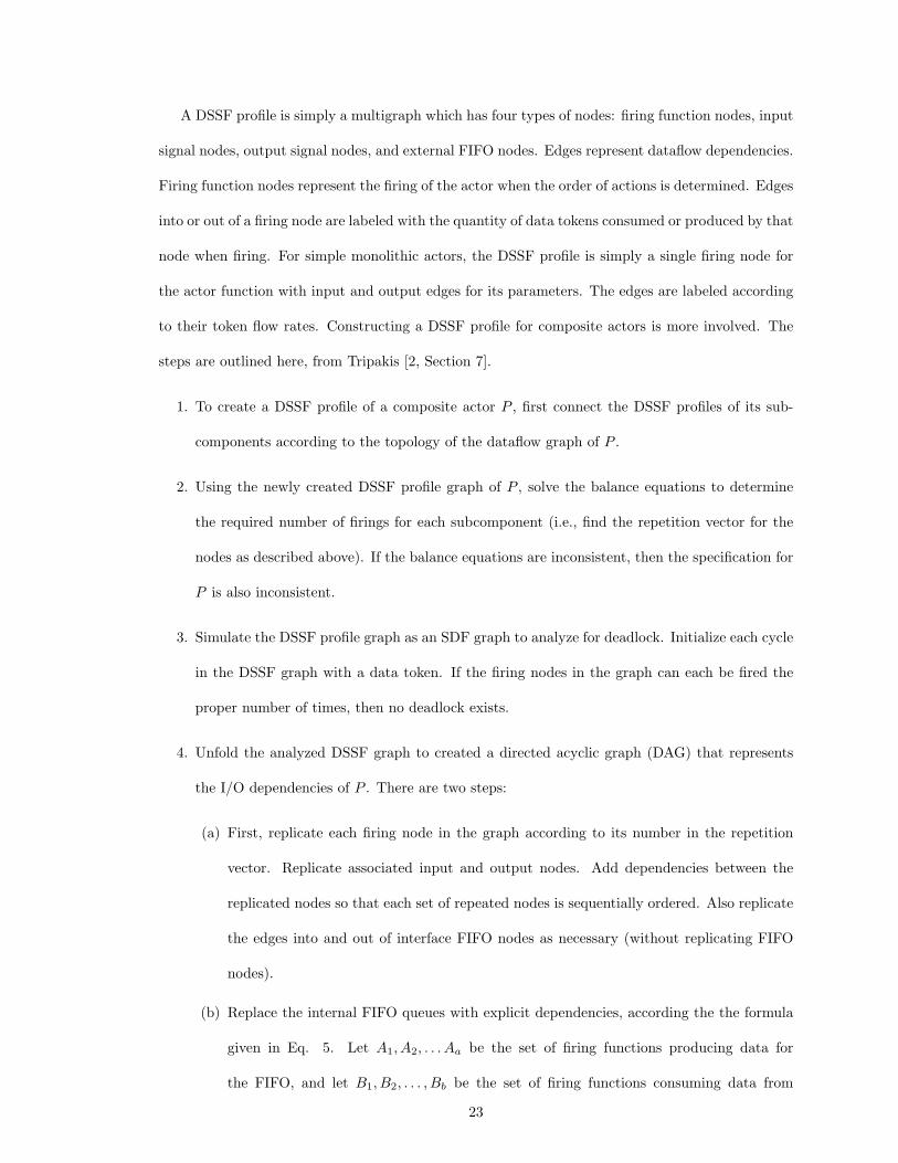
A DSSF profile is simply a multigraph which has four types of nodes: firing function nodes, input
signal nodes, output signal nodes, and external FIFO nodes. Edges represent dataflow dependencies.
Firing function nodes represent the firing of the actor when the order of actions is determined. Edges
into or out of a firing node are labeled with the quantity of data tokens consumed or produced by that
node when firing. For simple monolithic actors, the DSSF profile is simply a single firing node for
the actor function with input and output edges for its parameters. The edges are labeled according
to their token flow rates. Constructing a DSSF profile for composite actors is more involved. The
steps are outlined here, from Tripakis [2, Section 7].
1. To create a DSSF profile of a composite actor P , first connect the DSSF profiles of its sub-
components according to the topology of the dataflow graph of P .
2. Using the newly created DSSF profile graph of P , solve the balance equations to determine
the required number of firings for each subcomponent (i.e., find the repetition vector for the
nodes as described above). If the balance equations are inconsistent, then the specification for
P is also inconsistent.
3. Simulate the DSSF profile graph as an SDF graph to analyze for deadlock. Initialize each cycle
in the DSSF graph with a data token. If the firing nodes in the graph can each be fired the
proper number of times, then no deadlock exists.
4. Unfold the analyzed DSSF graph to created a directed acyclic graph (DAG) that represents
the I/O dependencies of P . There are two steps:
(a) First, replicate each firing node in the graph according to its number in the repetition
vector. Replicate associated input and output nodes. Add dependencies between the
replicated nodes so that each set of repeated nodes is sequentially ordered. Also replicate
the edges into and out of interface FIFO nodes as necessary (without replicating FIFO
nodes).
(b) Replace the internal FIFO queues with explicit dependencies, according the the formula
given in Eq. 5. Let A1, A2, . . . Aa be the set of firing functions producing data for
the FIFO, and let B1, B2, . . . , Bb be the set of firing functions consuming data from
23

the FIFO. These firing functions come from the DSSF profile graph before replicating
the instances. Now consider a particular producer and consumer pair, Av and Bu, where
v ∈ [1 . . . a] and u ∈ [1 . . . b]. In the instance-replicated graph, the ith instance of Av can be
written Av,i and the jth instance of Bu can be written Bu,j . Then for all combinations of
producer/consumer pairs (v, u) ∈ [1 . . . a]× [1 . . . b] and for each particular (v, u) consider
all of the instances (i, j) ∈ [1 . . . rAv ] × [1 . . . rBu ]. Then create a dependency directly
between Av,i and Bu,j if the following condition is satisfied:
d + (i− 1)∑a
h=1kh +
v−1∑h=1
kh
< (j − 1)∑b
h=1nh +
u∑h=1
nh
(5)
d represents the number of initial tokens in the FIFO. kh is the number of tokens produced
in the FIFO by actor Ah. nh is the number of tokens consumed from the FIFO by actor
Bh. If the link between an producing actor A and a consuming actor B is direct (i.e., no
explicit FIFO node exists between them), then repeat this procedure with a = b = 1 to
create the appropriate links between the instances.
The unfolded graph is used in the next step to get clusters that represent the firing functions of
a new DSSF profile for the whole component. Having separate firing functions means that the
abstracted component interface can be safely analyzed for deadlock without approximating.
5. Cluster the unfolded graph. The clusters are created so that no cyclic dependencies exist among
clusters. The DAG clustering algorithm given in [2] aims for maximum reusability, where no
false input-output dependencies will be created, and where the optimal (maximum) number
of clusters or more will be created using a greedy technique (since the optimal technique is
NP-complete). Clusters are also pairwise disjoint. Their algorithm is called greedy backward
disjoint clustering. Backward clustering means that the algorithm works from the outputs
backward. The result is a set of clusters C1, C2, . . . Cq which represent ’independent’ subsets
of dependencies for the component with respect to deadlock analysis.
24

6. Finally we create the new DSSF profile for the composite actor P . This step is somewhat
involved. Let Pc be the initial connected profile (from Step 1), let D be the unfolded graph,
let C = {Ci} be the set of clusters from the previous step, and let Pf be the new abstract
profile graph that we’re trying to create.
(a) In Pf , create an atomic firing node P.fi for each cluster Ci in C.
(b) For each input and output port of Pc, create a single FIFO. Each cluster writes to or reads
from the FIFOs at a rate specified by the sum of the actors in each cluster connected to
the FIFO. This can be determined from Pc, D, and the clusters Ci. If the rate is zero,
then the cluster is not connected to the corresponding FIFO.
(c) Create dependency edges in Pf between the firing nodes P.fi and P.fj if iff there exists
at least one edge between any node of Ci and any node of Cj .
(d) Consider each FIFO L in Pc. Let WL and RL be the ordered collection of clusters,
respectively, that write to and read from L. Create one dependency edge in each of WL
and RL from the last cluster to the first, with an initial token on the edge. This encodes
the requirement to wait to re-fire the cluster set until the last round has finished. If there
is only one cluster in either WL or RL, then do not create the additional edge.
(e) Now consider only the internal FIFOs of Pc (i.e., those not connected to an external port).
Suppose that a given internal FIFO L has d initial tokens. Let m be the number of tokens
produced by the clusters writing to L. m should also be the number of tokens consumed
by the reading clusters (by construction). Now we build a graph between the producer
and consumer clusters as follows: Let the ordered set z0, z1, . . . , zm−1 represent the tokens
produced by the clusters on the consumer side, ordered and partitioned according to the
cluster order and the number of tokens each cluster consumes. Likewise, create the ordered
set w0, w1, . . . , wm−1 for the producing clusters, similarly ordered and partitioned. For
i = 0 . . .m − 1, connect the cluster with token zi to the cluster with token wj , where
j = (d+ i) mod m. Also place bd+m−1−im c initial tokens for the edge associated with token
wi.
25

(a) Composite actor example for DSSFgeneration. Actors A and B are the com-ponents of composite actor H. Each inputand output port is labeled with the tokenflow quantity. The center edge has six ini-tial tokens.
(b) Unfolded graph. The dashed outlinesare one proposed clustering, and each is la-beled with its cluster number (Ci).
(c) Final DSSF profile. Unlike the graphcorresponding to the original diagram, thisrepresentation does not introduce false de-pendencies.
Figure 3: DSSF example graphs. Figs. from [2].
(f) Clean up the edges created in the last step as follows: remove all self-loops without initial
tokens, and then combine multiple edges between clusters by summing the initial tokens
and token flow values.
We take a simple example from [2, Fig. 10] to illustrate some of the steps in the technique. Fig.
II.3(a) shows a composite actor specification for which we would like to create a profile. After the
connection, unfolding, and clustering steps (1-N), we end up with the graph in Fig. II.3(b). This
is used to create the final profile (Fig. II.3(c)), which abstracts both token flow rate and deadlock
characteristics of the original composite actor H.
26

Compositional Stability Analysis
Compositional techniques in control systems analysis seek to verify stability of a design model us-
ing component properties and interconnection rules. Robust control techniques consider feedback
interconnections of components, seeking to characterize and formalize behavior properties of the
connected components when one or both of the components are perturbed. Teel briefly describes
the development of the robust control approach for stability [54, Section IV]. The robust approach
centers on the explicit modeling of uncertainty in system inputs and parameters, along with tech-
niques for analyzing and optimizing interconnected systems designs that include uncertainties[55].
Passivity is a property of control system behavior that implies stability, composes under particular
interconnections of components, and which reduces the destabilizing effects of data and parameter
quantization [10] as well as delays due to digital processor scheduling and network communications
[56] [57].
Passive Control Design
Let Ein, Eout represent energy input and output for a component. Passivity means that energy
output for a particular component never exceeds its energy input together with any remaining
stored energy. Passive systems are compositional, as discussed below. Bounded-input bounded-
output (BIBO) stability requires Eout ≤ KEin. BIBO stability follows directly from passivity, but
is very weak in terms of our ability to direct the trajectory of the controlled system. Asymptotic
stability is a stronger form of stability that implies convergence of the system trajectories to a
particular point. If the system can be structured to provide a reference trajectory, then asymptotic
stability permits trajectory tracking. Usually a search for a Lyapunov function is used to establish
asymptotic stability for an arbitrary nonlinear system. Lyapunov functions generally represent (or
bound) the behavior of the entire system, so they are not compositional. Passivity can be used to
compositionally establish asymptotic stability with a few more strictness constraints.
To establish passivity for linear system models, Kottenstette gives Linear Matrix Inequality(LMI)
conditions to verify passivity of a linear time-invariant system in state-space form[58] (Eq. 6). If
a positive definite solution Pi exists satisfying the given matrix inequality, then the component is
27

passive. The inequality is interpreted in the sense of semidefinite programming, where for example
M ≤ 0 means “matrix M is negative semidefinite”[59]. Further constraining the matrix P to be
symmetric, we can solve this LMI efficiently using convex optimization techniques[60].
ATi Pi + PiAi PiBi − 1
2CTi
BTi Pi − 1
2Ci − 12 (DT
i CTi + CiDi)
≤ 0 (6)
Desoer and Vidyasagar give frequency domain conditions for passivity for LTI system models[61].
For continuous-time:
H is passive iff H(jω) + H∗(jω) ≥ 0, ∀ω ∈ R.
For discrete-time:
H is passive iff H(ejθ) + H∗(ejθ) ≥ 0, ∀θ ∈ [0, π].
Sector Analysis
Using the formulation in Zames[62], the sector bounds for a possibly nonlinear control component
are a real-valued interval [a, b], where the endpoints come from the expression in Eq. 7.
‖yT ‖22 − (a + b)〈y, u〉T + ab‖uT ‖22 ≤ 0 (7)
For linear (and some nonlinear) system models, sector bounds may be computed symbolically
during system analysis. Each component is assigned a real interval ([a, b] −∞ < a ≤ b ≤ ∞, b ≥
0) representing a range of possible input/output behaviors. Components whose bounds fall in
the interval [0,∞] are passive (and have some notion of stability). Zames also presents rules for
computing sector bounds for systems based on calculated component bounds and different types of
interconnections between components [62]. We describe the sector formulas, rules, and bounds in
greater detail below.
From [62] and [63], another way to look at Eq. 7 is the following formulation. A system
H, (y = Hx) is inside the sector [a, b] if a ≤ b and
〈(Hx)t − axt, (Hx)t − bxt〉 ≤ 0 (8)
28

Where 〈· · · , · · · 〉 is the inner product on the appropriate function space.
Most approaches to nonlinear control system design rely on continuous time assumptions. When
we consider discrete time implementation in software subject to network delays and finite-precision
quantization effects, linear approximations and high sample rates are used to obtain tractable anal-
ysis and realizable execution. In practice we have found that compositional techniques based on
passivity have allowed us to construct reasonably low data rate digital controllers for nonlinear
systems without resorting to conservative linear approximations[64].
Passive control techniques have proven successful for many cases of nonlinear continuous time
controllers, but nonlinear discrete time control poses several challenges. Unfortunately many control
structures are not passive in discrete time. If we can approximate our controlled system as a cascade
of passive systems then we can apply a systematic control design strategy, for which stability can
be validated online.
Digital control for nonlinear physical systems with fast dynamics (such as a quadrotor helicopter)
use a zero-order hold to convert control values produced at discrete time instants into step functions
held over a continuous interval of time. For certain inputs and state trajectories, the hold process can
introduce small amounts of new energy into the environment, violating passivity. The sector bounds
analysis proposed by Zames [62] can be used to assess the amount of “active” (energy-producing)
behavior which we can expect from a design under nominal operating conditions.
Zames’ critical insight was that many causal nonlinear systems’ dynamic input-output relation-
ships can be confined to being either inside or outside a conic region. Systems whose input-output
relationships can be confined inside a conic region are known as interior conic systems. Equivalently
these interior conic systems can be described as residing inside the sector [a, b] in which a and b
are real coefficients[62]. If there exist a real coefficients a and b such that Eq. 7 is satisfied then
the system is an interior conic system inside the sector [a, b] conversely if the inequality of Eq. 7 is
reversed the system is exterior conic and outside the sector [a, b]. Table 3 describes the quantities
used in Eq. 7. For linear time invariant (LTI) single input single output (SISO) systems the term
a is the most negative real part of its corresponding Nyquist plot, it therefore is an approximate
measure of the phase shift of a stable system. A passive system is equivalent to an interior conic
29

Figure 4: Block diagram interconnection examples for conic system composition rules.
30

Quantity Descriptionu(t) Input signaly(t) Output signal
Energy produced by the component so far‖yT ‖22 (output) in a time interval of length T .
Energy received by the component so far‖uT ‖22 (input) in a time interval of length T .
Correlation between the input and output〈y, u〉T sample values in a time interval of length T .
This is a measure of dissipation.a Real-valued lower bound for the sector.b Real-valued upper bound for the sector.
Table 3: Quantities for the sector formula.
system which is inside the sector [0,∞] therefore a passive LTI SISO system has no more than +/-90
degrees of phase shift in which all real parts of its corresponding Nyquist plot are positive real.
A conic system can also be modeled as a functional relation between the possible input and
output signal spaces. This corresponds intuitively to a causal block diagram where the function
specified in the block relates the inputs to the outputs, as in Fig. 4 (a). See Zames for a complete
formal functional description of sector analysis. Given conic relations H,H1 with H in [a, b] and H1
in [a1, b1] (b, b1 > 0), and given a constant k ≥ 0, we have the following sector composition rules
from [62]:
1. I is in [1, 1] (Fig. 4 (b))
2. kH is in [ka, kb] (Fig. 4 (c))
3. −H is in [−b,−a] (Fig. 4 (d))
4. sum rule H + H1 is in [a + a1, b + b1] (Fig. 4 (e))
5. inverse rule(s) (Fig. 4 (f))
(a) a > 0→ H−1 is in [ 1b , 1a ].
(b) a < 0→ H−1 is outside [ 1a , 1b ].
(c) a = 0→ (H−1 − ( 1b I)) is positive.
For rule 5 an inverse system model must be well-defined (i.e. exist), as in the case of invertible
linear system models.
31

Figure 5: Block diagram interconnection example for feedback structure.
The sector composition rules illustrate the compositional nature of sector analysis. Zames also
gives conditions under which feedback-interconnected conic systems exhibit stability [62, Theorems
2a,2b]. We will not describe all of the details here, but simply relate the sufficient condition described
in Kottenstette to establish stability of feedback control loops where the included systems are conic
[65, Corollary 2]:
Assume that the combined dynamic system H : [u1, u2] → [y1, y2] depicted in Fig. 5 consists
of two dynamic systems H1 : u1 → y1 and H2 : u2 → y2 which are respectively inside the sector
[a1, b1] and strictly inside the sector [0, 1 + ε], for all ε > 0. Then H is bounded (Lm2 stable for the
continuous time case or lm2 stable for the discrete time case) if:
− 1max{|a|, b}
< k < − 1a1
, if a1 < 0
−1b
< k <∞, otherwise.
In order to design with sectors, it is important to be able to relate sector conditions for continuous-
time systems with those for discrete-time systems. Kottenstette et al introduce a linear discretization
operator called the IPESH -transform (Inner Product Enhanced Sample and Hold) that preserves
sector conditions during discretization[12]. Briefly put, the IPESH -transform guarantees that a
continuous-time conic system Hct that is inside a sector [a, b] that is discretized using IPESH at a
sample rate of Ts, then the resulting filter will lie in the sector [aTs, bTs] [12, Lemma 3]. Finally, we
give the form for the transformation (Eq. 9).
32

Hp(z) =(z − 1)2
TszZ{Hp(s)
s2} (9)
Sector analysis extends our analysis capabilities to many nonlinear and non-passive system mod-
els and control structures. As discussed in the previous section, the mathematical framework by
itself is not sufficient to support incremental design analysis. We must deal with partitions of the
design into interfaces and the relationships of various control loops to each other and to the plant
dynamics. This is an open problem in modeling, and sector analysis is one candidate for a formal
analysis framework which could support incremental design and analysis tools.
Passivity and Platform Effects
Modern passive control techniques demonstrate that passive systems exhibit insensitivity to platform
effects. We will briefly cover a few of these results.
1. Quantization errors Perhaps the best passivity-based framework for quantization effects
is described by Fettweis [10]. Physically realizable passive circuit models are used to derive
compositional digital filter structures with similar passivity constraints.
2. Sampling rate variations (IPESH/multi-rate) Kottenstette presents a technique for dis-
cretizing filters which is less sensitive to changes in sampling rate (IPESH transform) [11]. He
also presents a method for constructing passive networked control designs where individual
components operate at different rates [12].
3. Network delays For communication delays, Anderson and Spong [66] derived passivity condi-
tions for a particular networked control configuration. The two-port scattering matrix formu-
lation make the delay analysis tractable, as it appears as a two-port component in the center of
the control structure. From this they derive passivity conditions. Their digital implementation
was unstable for large time delays. The control analysis used continuous-time models, and a
naive application of discretization.
Niemeyer and Slotine extended the work of Anderson using the observation that physical
waves transmit energy in a stable manner[13]. They introduced discrete wave variables, which
33

surprisingly removed the delay term from the original formulation. This led to a much more
general framework for handling communications in passive control designs. Wave variables
redistribute the values of the effort and flow at a port consistent with the distributed effort
and flow that a wave would use to transmit energy between two points.
34

CHAPTER III
THE EMBEDDED SYSTEMS MODELING LANGUAGE (ESMOL)
Consider the general class of control system designs for use in a flight control system. Sensors,
actuators, and data networks are designed redundantly to mitigate faults. The underlying platform
implements a variant of the time-triggered architecture (TTA) [50], which provides precise timing and
reliability guarantees. Safety-critical tasks and messages execute according to strict precomputed
schedules to ensure synchronization between replicated components and provide fault mitigation
and management. Deployed software implementations of the control functions must pass strict
certification requirements which impose constraints on the software as well as on the development
process. The additional burden of design analysis required to establish safety increases cost and
schedule, decreasing the flexibility of the development process.
In modern embedded control system designs, graphical modeling and simulation tools (e.g. Math-
works’ Simulink/Stateflow) represent physical systems and engineering designs using block diagram
notations. Design work revolves around simulation and test cases, with code generated from models
when the design team reaches particular schedule milestones. Control designs often ignore software
design constraints and issues arising from embedded platform choices. At early stages of the design,
platforms may be vaguely specified to engineers as sets of trade offs [67].
Software development uses Unified Modeling Language Computer-Aided Software Engineering
(UML CASE) tools to capture concepts such as types, components, interfaces, interactions, timing,
fault handling, and deployment. Software development work flows focus on source code creation,
organization, and management, followed by testing and debugging on target hardware. Physical and
environmental constraints are not usually represented by the tools. At best such constraints may be
provided as documentation to developers.
Complete control system software designs rely on multiple aspects. Designers lack tools to model
the interactions between the hardware, software, and the environment with the required fidelity. For
example, software generated from a carefully simulated synchronous dataflow model of the controller
35

functions may fail to perform correctly when its functions are distributed over a shared network of
processing nodes. Cost or availability considerations may force the selection of platform hardware
that limits timing accuracy or data precision beyond originally designed bounds. None of the current
design, analysis, or development techniques support comprehensive (i.e. multi-domain) validation
of certification requirements to meet government safety standards. Model and code analysis tools
must all be integrated to have the same semantic view of the design details.
Overview
We aim to create a Domain Specific Modeling Language (DSML) to address problems of design
consistency across the entire development flow for a distributed embedded control system design.
Often, the best solutions involve iterating the design cycle as problems are discovered or problem
understanding increases. Our DSML captures the relationships between concepts in the different
design domains described, and supports the integration of analysis tools and code generation.
High-Confidence Design Challenges
We identify several specific challenges that arise because of inconsistencies between domains in a
high-confidence embedded development project. Some of the challenges are fundamental, and others
arise because of our attempts to use models to resolve consistency problems.
1. Controller, software, and hardware design domains are highly specialized and often conceptu-
ally incompatible. Sharing model artifacts between designers in different domains can lead to
consistency problems in engineering solutions or implementations based on incomplete or faulty
understanding of design issues. Current state of the art resolves differences in understanding
by reviewing many of the details in numerous meetings and personal discussions. Manual rec-
onciliation of issues occurs as individual designers receive assignments to modify and correct
the design. In the worst cases serious incompatibilities are not discovered until very late in
the design cycle, leading to project overruns and cancellations[4]. Several large modeling tool
projects (for example, AADL [14] and Topcased[21]) work to integrate tools from independent
research and development teams into a common design environment featuring a standardized
36

modeling language. Resolution of semantic consistency between integrated tools to improve
design efficiency is a serious issue in such efforts.
2. Incompatibilities between models and assumptions in different design domains create a related
problem. For example, controller design properties which are verified using simulation models
may no longer be valid when the design becomes software in a distributed processing net-
work. Currently control designers use conservative performance margins to avoid rework when
performance is lost due to deployment on a digital platform.
3. Long development, deployment, and test cycles limit the amount of iterative rework that can
be done to get a correct design. If a particular design analysis is costly or time-consuming,
the team cannot afford to iterate the design from its early stages in order to resolve problems.
Currently high-confidence design requires both long schedules and high costs.
4. Automating steps in different design and analysis domains for the same models and tools
requires a consistent view of inferred model relationships across multiple design domains. If
integrated tools have different views of the model semantics, then their analyses are not valid
when the results are integrated into the same design. Therefore, all of the tools used in the
design process must have a consistent view of design details. Explicitly reconciling semantics
between formalisms and tools is costly and time-consuming. Often the effort cannot be justified
outside of academic research unless the results are applicable to numerous designs.
5. As our research explores new directions in high-confidence design, modification of the ESMoL
meta-model (language specification) creates maintenance problems for ESMoL models and for
interpreter code that translates them into analysis artifacts and generated code. We would like
to isolate interpreter development from the language to a degree in order to allow the ESMoL
language to evolve with our research. ESMoL models can be updated to new versions of the
language using features built into the tools, but nothing exists yet to handle those problems
for interpreter code.
37

Model-Integrated Solutions
We propose a suite of tools that aim to address many of these challenges. Currently under develop-
ment at Vanderbilt’s Institute for Software Integrated Systems (ISIS), these tools use the Embed-
ded Systems Modeling Language (ESMoL), which is a suite of domain-specific modeling languages
(DSML) to integrate the disparate aspects of a safety-critical embedded systems design and main-
tain proper separation of concerns between control engineering, hardware specification, and software
development teams. The Embedded Systems Modeling Language (ESMoL) encodes in models the
relationships between controller functions specified in Simulink, software components that imple-
ment those functions (i.e. dataflow, messaging interfaces, etc. . . ), and the hardware platform on
which the software will run. Many of the concepts and features presented here also exist separately
in other tools. We describe a model-based approach to building a unified model-based design and
integration tool suite which has the potential to go far beyond the state of the art.
1. The ESMoL language and tools provide a single multi-aspect embedded software design envi-
ronment so that modeling, analysis, simulation, and code generation artifacts are all clearly
related to a single design model. We aim to incorporate models appropriate to the different
design domains in a consistent way using the Model-Integrated Computing (MIC) approach
discussed below. ESMoL models use language-specified relations to associate Simulink control
design structures with software and hardware design concepts to define a software implemen-
tation for controllers. Further, ESMoL is a graphical modeling language which integrates into
existing Simulink-based control design work flows[68].
2. ESMoL models include objects and parameters to describe deployment of software components
to hardware platforms. Analysis artifacts and simulation models generated from ESMoL mod-
els contain representations of the behavioral effects of the platform on the original design. We
include platform-specific simulations to assess the effects of distributed computation on the
control design [69].
3. ESMoL’s integrated analysis, simulation, and deployment capabilities can shorten design cy-
cles. The ESMoL tool suite includes integrated scheduling analysis tools which converge quickly
38

in most cases ([70]) so that static schedules can be calculated in rapid design and simulation
cycles. We include automatic generation of platform-specific task configuration and data com-
munications code in order to rapidly move from modeling and analysis to testing on actual
hardware.
4. ESMoL uses a two-stage interpreter architecture in order to integrate analysis tools and code
generators. The first stage resolves any inferred model relationships from ESMoL models into a
model in an abstract language (ESMoL Abstract), much in the same way that a parser creates
an abstract syntax tree for a program under compilation. The ESMoL design language allows
relational inference where appropriate in order to make the user experience more productive.
The Stage 1 interpreter resolves object instances, parameters, and relations, and stores them
in an ESMoL Abstract model. Model interpreters for analysis and generation use this ex-
panded model to guarantee a consistent view of the relationships and details, and to share
code efficiently in an integrated modeling tool development project. The two-stage approach
also isolates the interpreter code from the structure of the ESMoL language. Changes to the
language are principally isolated from the interpreter code by the first stage transformation.
5. We generate analysis models and code from the intermediate language using simple template
generation techniques[70]. Round-trip incorporation of calculated schedule analysis results
back into the ESMoL model helps to maintain consistency as models pass between design
phases.
Fig. 6 depicts a design flow that includes a user-facing modeling language for design and an
abstract intermediate language for supporting interpreter development and maintenance. During
design, a software modeler imports an existing Simulink control design into the Generic Modeling
Environment (GME) [71], configured to edit ESMoL models (Step 1). The modeler then uses the
dataflow models imported from Simulink to specify the functions of software components which
will be used to implement the controllers. These component specifications represent synchronous
dataflow models that are realized as C code calls, and which are extended with interfaces defining in-
put and output message structures for data distribution. We also specify the mapping from dataflow
39

Figure 6: Flow of ESMoL design models between design phases.
40

I/O ports to and from fields in the messages (Step 2). Designers specify the hardware topology for a
time-triggered distributed processing network using another integrated design language (Step 3). A
modeler instantiates component instances to create multi-aspect models where logical dependencies,
hardware deployment, and timing models can be specified for the software architecture (Steps 4 and
5).
A completed model is transformed (via the Stage 1 transformation) into a model in the ES-
MoL Abstract language, resolving all implied relationships and structural model inferences (Step
6). Model interpreters for design analysis (in this case calculating time-triggered schedules) are
integrated using the Stage 2 model transformation from ESMoL Abstract models to analysis specifi-
cations (Step 7). Another model interpreter imports results from the analysis (in this case, scheduled
start times) back into the ESMoL Abstract and ESMoL models (Steps 8 and 9). Finally, design-
ers can also create platform-specific simulations and generate deployable code using the Stage 2
transformation (Step 10).
In a later section we discuss the relationship between the behavior represented by the original
Simulink model and the behaviors represented by ESMoL and ESMoL Abstract (Steps 5 and 10).
ESMoL provides a great deal of modeling flexibility, as subsets of the Simulink model are used
in Step 2 to define software components. These subsets can be replicated to model redundant
computation networks, for example. In Step 4 they are aggregated to define dataflows, and then
partitioned to define deployment of those dataflows. With all of the language flexibility provided, we
need to ensure that the synchronous semantics of the original Simulink model are preserved in the
distributed implementation in order to ensure that the inherent correctness properties (functional
determinism, timing determinacy, and deadlock freedom) are also preserved.
The illustrated design flow represents only a single iteration in the overall development work flow
to be discussed later. In the sequel we will use the expression design flow to indicate the work of
modeling, analyzing, and generating code for a single design. Development flow will indicate the
macro-level iterative development process which includes one or more design flow iteration.
41

Figure 7: Platforms. This metamodel describes a simple language for modeling the topology of atime-triggered processing network.
Tools and Techniques
The models in the example and the metamodels described below were created using the ISIS Generic
Modeling Environment tool (GME) [71]. GME allows language designers to create stereotyped
UML-style class diagrams defining metamodels. The metamodels are instantiated into a graphical
language, and metamodel class stereotypes and attributes determine how the elements are presented
and used by modelers.
The Model-Integrated Computing (MIC) approach[5] builds up DSMLs by creating specific sub-
languages to capture concepts and relationships for different facets of the design domain, and then
integrating those sublanguages into a common modeling language by precisely specifying the struc-
tural relationships between those sublanguages. In a GME metamodel a sublanguage is called a
paradigm. We will use the terms sublanguage, language, and paradigm interchangeably. Confusion
is resolved by explicitly naming the paradigms involved in the discussion.
The GME metamodeling syntax may not be entirely familiar to the reader, but it is well-
documented in Karsai et al [71]. Class concepts such as inheritance can be read analogously to
UML. Class aggregation represents containment in the modeling environment, though an aggregate
42

element can also be flagged as a port object. In the modeling environment a port object will also
be visible at the next higher level in the model hierarchy, and available for connections. One unique
notation in MetaGME (the GME modeling language for creating modeling languages) is the dot used
for relating an association class to its endpoint connection classes. For example, the dot between
the Connectable class and the Wire class (Fig. 7) represents a line-style connection in the modeling
environment. One other useful concept from a GME metamodel is the reference. A reference object
appears in the Metamodel specification associated with another class. This allows the modeler to
create an object with the same interface (port structure) as the associated class, but which actually
refers to the original object, much in the same way that a pointer refers to a different object in
memory in a computer program.
Another key technology used in the ESMoL tool suite is the GReAT model transformation lan-
guage (and its associated code generation tools)[72]. The ESMoL suite contains a pair of platform-
independent code generators for Simulink and Stateflow models. The transformations take Simulink
and Stateflow blocks, and create equivalent models in another language (SFC) that corresponds to
an abstract syntax graph for fragments of C code. Functional code generation proceeds by simply
traversing and printing the SFC models. Other generators use the UDM C++ modeling API [73]
to create code implementing the platform-specific code to wrap functions as tasks, define communi-
cation messages structures, and configure a time-triggered virtual machine to execute the generated
code. These generators as well as generators for platform-resimulation models are described else-
where (see Porter et al [68], Thibodeaux [74], and Hemingway et al [69] for details).
Platform-based design partitions design frameworks into designer-supplied components and plat-
form-provided services[67]. High-confidence systems require services and guarantees for correct and
efficient execution such as real-time execution, data distribution, and fault tolerance. Platform-
based design allows the construction of complex systems by facilitating reuse over common execution
behaviors. The platform also defines a formal model of computation (MoC) [75], which predicts how
the concurrent objects of an application interact (i.e. synchronization and communication). We use
an implementation of the time-triggered architecture as a platform layer in order to reduce timing
variances in sensing, actuation, and distributed data communications [50][74]. The central idea of
43
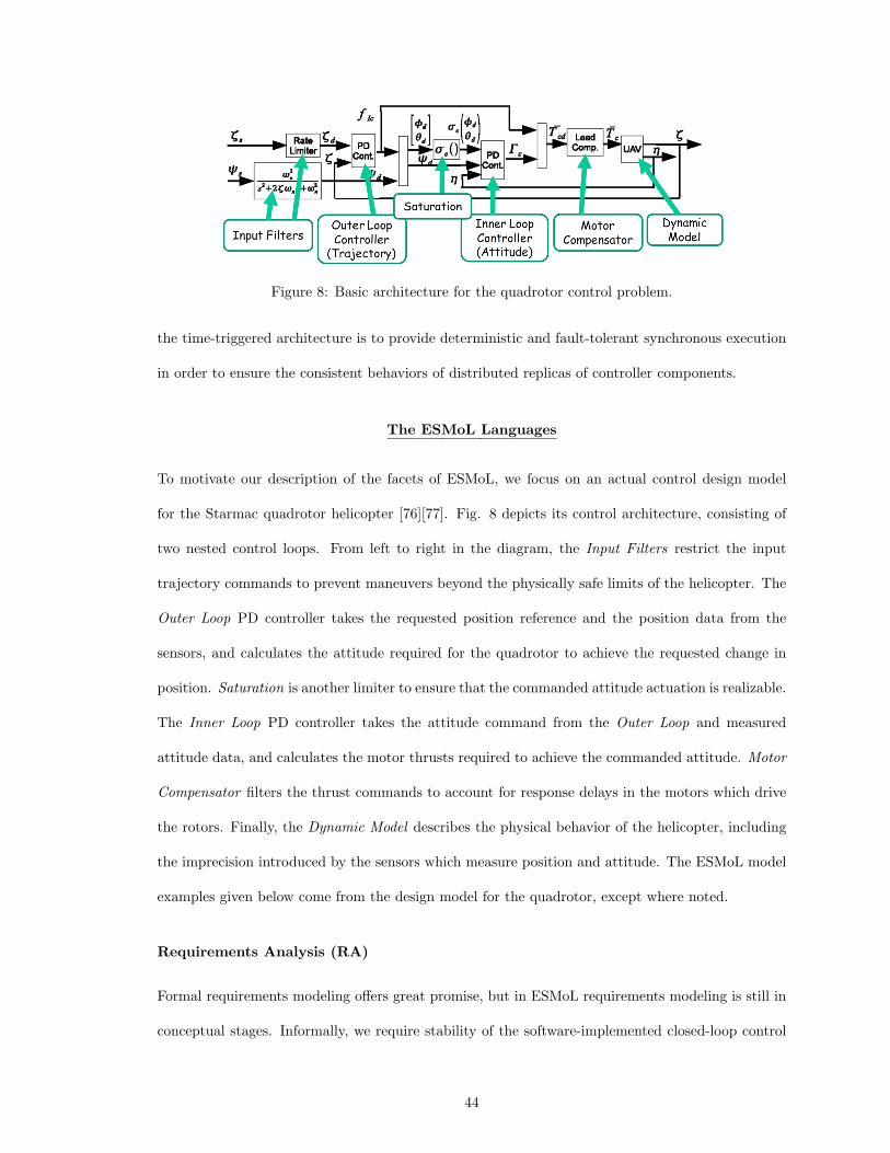
Figure 8: Basic architecture for the quadrotor control problem.
the time-triggered architecture is to provide deterministic and fault-tolerant synchronous execution
in order to ensure the consistent behaviors of distributed replicas of controller components.
The ESMoL Languages
To motivate our description of the facets of ESMoL, we focus on an actual control design model
for the Starmac quadrotor helicopter [76][77]. Fig. 8 depicts its control architecture, consisting of
two nested control loops. From left to right in the diagram, the Input Filters restrict the input
trajectory commands to prevent maneuvers beyond the physically safe limits of the helicopter. The
Outer Loop PD controller takes the requested position reference and the position data from the
sensors, and calculates the attitude required for the quadrotor to achieve the requested change in
position. Saturation is another limiter to ensure that the commanded attitude actuation is realizable.
The Inner Loop PD controller takes the attitude command from the Outer Loop and measured
attitude data, and calculates the motor thrusts required to achieve the commanded attitude. Motor
Compensator filters the thrust commands to account for response delays in the motors which drive
the rotors. Finally, the Dynamic Model describes the physical behavior of the helicopter, including
the imprecision introduced by the sensors which measure position and attitude. The ESMoL model
examples given below come from the design model for the quadrotor, except where noted.
Requirements Analysis (RA)
Formal requirements modeling offers great promise, but in ESMoL requirements modeling is still in
conceptual stages. Informally, we require stability of the software-implemented closed-loop control
44

system over the full range of possible inputs, and satisfaction of the calculated timing constraints
(task release times and deadlines).
Functional Design (FD)
In ESMoL, functional specifications for components can appear in the form of Simulink/Stateflow
models or as existing C code snippets. ESMoL does not support the full semantics of Simulink. In
ESMoL the execution of Simulink data flow blocks is restricted to periodic discrete time, consistent
with the underlying time-triggered platform. This also restricts the type and configuration of blocks
that may be used in a design. Continuous integrator blocks and sample time settings do not have
meaning in ESMoL. C code snippets are allowed in ESMoL as well. C code definitions are limited
to synchronous, bounded response time function calls which will execute in a periodic task with a
fixed amount of memory.
An automated importer constructs an ESMoL model from a Simulink control design model. The
new model is a structural replica of the original Simulink model, only endowed with a richer software
design environment and tool-provided APIs for navigating and manipulating the model structure
in code. The Simulink and Stateflow sublanguages of our modeling environment are described
elsewhere[78]. The ESMoL language evolved from another DSML known as ECSL-DP. They share
many concepts, but ESMoL departs from many of the modeling structures previously described by
Neema in order to increase the flexibility and generality of the language.
Component Design (CD)
In the component design phase (CD) we specify software interfaces for the functions which will run
in the distributed controller network. A component type has a unique name (i.e. InnerLoop), and
information to find or generate its implementation in C (in this case, the file name and model path to
the Simulink subsystem “QuadRotor/STARMAC/InnerLoop”). A component specification contains
a reference to a Simulink subsystem, as well as references to message structure objects. The message
structure objects will represent message types, and each reference from a component definition
represents an interface through which that message is sent or received. Internally, the direction of
45

Figure 9: Quadrotor component types model from the SysTypes paradigm.
the connection from the message reference to the ports on the Simulink object determine whether
the port sends or receives. We do not allow multi-directional message transfers on the same interface.
When the component is instantiated in the design model (e.g., in the logical architecture diagram
described below) the message references specified here will appear as ports on blocks representing
the instance. Connections to and from those ports represent the transfer of an instance of that data
message into or out of the component instance.
Fig. 9 shows an example of a model from the component interface definition language. Message
fields and their sizes are specified here, as well as component implementations and interfaces. These
specifications define software component types in an ESMoL model, which are instantiated and
assigned to hardware in the architecture and deployment models, respectively. The quadrotor model
has four different component types (each instantiated once) and six message types (instantiated as
the ports objects appearing on the component instances later in the design). The breakout inset
in the figure shows the internals of the DataHandler component specification. The sensor convert
subsystem block in the center is a reference to a Simulink block specifying the data conversions that
transform raw sensor data into scaled, formatted data for use by the controller blocks.
46

Figure 10: SystemTypes Metamodel.
The blocks on the outer edges of the figure (Fig. 9) are references to messages defined at the
top level of the system types model. On the left is the raw data message from the sensors. On the
right are the attitude data message (for local consumption by the inner loop), and the position data
message (sent remotely to the outer loop). The three message reference blocks in the inset appear
as ports on the DataHandler block (top left in the figure). Inside the component type definition,
ports on the message objects correspond to C structure fields. The field types are inferred from the
data types imported from the connected Simulink signal port objects. The connections between the
message ports and the Simulink reference block ports describe the direction and details of data flow
between the implemented message structures and the specified functional block.
Fig. 10 portrays the SystemTypes sublanguage, which encodes these structures and relations.
Components of different types (here Simulink block references or C code blocks) specify the compo-
nent functions. Message references (MessageRef objects) define interfaces on the components, and
ports on message objects (MsgPort objects) represent message data fields as in the DataHandler
47

Figure 11: Overall hardware layout for the quadrotor example.
example. The Input and Output port classes are typed according to the implementation class to
which they belong (i.e., either Simulink signal ports or C function arguments). The connections
between the block reference and the MsgPort objects describe the details required to marshal and
demarshal the data fields in the messages for use by the specified function. Synchronous, periodic,
discrete-time Simulink blocks and bounded-time synchronous C function calls are compatible at this
modeling stage, because their model elements both represent the code that will finally implement
the functions. These units are modeled as blocks with ports, where the ports represent parameters
passed into and out of C function calls. The Trigger and Event types are not discussed here, as
they relate to future work in the ESMoL tool suite.
Hardware Architecture (HwA)
Fig. 11 illustrates the example platform model. The quadrotor architecture is deployed to a small
embedded processor assembly manufactured by Gumstix, Inc. The outer loop position control is
handled by an Intel PXA ARM processor (the Gumstix board), and attitude control and vehicle
I/O are handled by an Atmel Atmega128 AVR processor (the Robostix board). The I/O occurs over
serial connections to the sensors and motor actuators. The serial devices reside within the processor,
and are modeled in the diagram as objects connecting the input and output ports on the processor
to the object representing the plant dynamics. The two processors communicate via a synchronous
I2C bus which runs a software emulated time-triggered protocol.
48

A simple platform definition language (Fig. 7) contains relationships and attributes describing
time-triggered networks. The models contain network topology and parameters to describe behav-
ioral quantities like data rates and bus transfer setup times. Platforms are defined hierarchically
as hardware units with ports for interconnections. Primitive components include processing nodes
and communication buses. Behavioral semantics for these networks come from the underlying time-
triggered architecture. The time-triggered platform provides services such as deterministic execution
of replicated components and timed message-passing. Model attributes for hardware also capture
timing resolution, overhead parameters for data transfers, and task context switching times.
Architecture Language
Logical architecture, deployment, and timing/execution models represent different design aspects
for the same set of component instances. GME allows us to define the language in such a way that
these three model aspects are simply different views of the same set of model elements. Together,
the information in the three aspects define a model which is complete with respect to scheduling
analysis, platform-specific simulation, and code generation.
System design models defined in the architecture language do not necessarily represent complete
designs. For simple designs (such as the quadrotor example) a single architecture model can cap-
ture all of the details of the software model. More complex designs require an additional layer of
organization which is not described here. It suffices to say that designs represented in the ESMoL
Architecture language can be considered as fragments which can be assembled into more complex
structures. This is an active area of research for our ESMoL modeling efforts, as the higher-level
architecture models should also account for fault modeling, evaluation, and performance issues.
• Logical Software Architecture (SwA) Aspect Fig. 12 portrays an ESMoL model ex-
ample specifying logical data dependencies between quadrotor software component instances,
independent of their distribution over different processors. The software architecture model
describes the logical dataflow dependency relationships between component instances. Seman-
tics for SwA Connections are those of task-local synchronous function invocations (with shared
49

Figure 12: Quadrotor architecture model, Logical Architecture aspect.
memory messaging) or message transfers between remote tasks using time-triggered commu-
nication. In this model the interpretations for the dependency links have not been specified.
Those details appear in the deployment model.
For the quadrotor, the RefHandler and DataHandler components receive and process data from
the sensors. They pass their formatted data to the respective control blocks. The OuterLoop
calculates an attitude reference to achieve the requested position. The InnerLoop issues thrust
commands to achieve the requested attitude.
In a design model, creation of a (GME) reference object to one of the component types cor-
responds to instantiation. Fig. 13 illustrates this idea. Using the same controller components
along with a few new components to implement voting logic, we have specified the logical
architecture for a triply-redundant version of the quadrotor model. Each ESMoL component
type is used multiple times in a single design, expanding the model structure far beyond the
size and scope of the original Simulink design. This particular model diagram is only shown
to illustrate the instantiation mechanism.
• Deployment Models (SY, DPL) Fig. 14 displays the deployment model – the mapping of
software components to processing nodes, and data messages to communication ports. Two
of the four components are mapped to each of the two processors. For the quadrotor, the
RefHandler and OuterLoop tasks run on the Gumstix processor. The InnerLoop and Data-
Handler tasks run on the Robostix processor. RefHandler receives position commands from a
socket connection. DataHandler receives sensor data from a UART channel (a processor port
50

Figure 13: Triply-redundant quadrotor logical architecture. This is not part of the actual quadrotormodel, and is only given for illustration.
Figure 14: Quadrotor architecture model, Deployment aspect.
51

Figure 15: Details from the deployment sublanguage.
in the model diagram). Position and attitude data are exchanged over the time-triggered bus,
so the corresponding message ports are connected to bus channel objects on their respective
processors. InnerLoop sends thrust commands through a UART channel, hence the connection
to the appropriate processor port.
In the figure the dashed connection from a component to a node reference represents an
assignment of that component to run as a task on the node. The port connections represent
the hardware channel through which that particular message will travel. Remote message
dependencies are assigned to bus channels on the node. Local data dependencies are not
specified here, as they are represented in the logical architecture. IChan and OChan port
objects on a node can also be connected to message objects on a component. These connections
represent the flow of data from the physical environment through sensors (IChan objects) or the
flow of data back to the environment through actuators (OChan objects). Model interpreters
use deployment models to generate platform-specific task wrapping and communication code
as well as scheduling problem specifications.
The metamodel in Fig. 15 illustrates the classes and relationships for both the logical architec-
ture connections and the deployment mapping. GME metamodels have a separate visualization
aspect that allows us to define aspects in ESMoL and indicate which classes and connections
should be visible in each aspect. ComponentRef objects are software component instances, and
are visible in both aspects. In the logical architecture aspect, Dependency connectors define
52

Figure 16: Quadrotor architecture model, Timing aspect.
message transfers between component instance ports. The ports represent interfaces for each
component instance. For the deployment aspect we add NodeRef objects (node references)
and connectors (ComponentAssignment and CommMapping) to identify the mapping of tasks
and messages to the platform model.
The deployment aspect captures the assignment of component instances as periodic tasks
running on a particular processor. In ESMoL a task executes on a processing node at a single
periodic rate. All components within the task execute synchronously. Data sent between tasks
take the form of messages in the model. For data movement, the runtime provides logical
execution time semantics found in time-triggered languages such as Giotto [79] – message
transfers are scheduled after the deadline of a sending task, but before the release of the
receiving tasks. Tasks never block, but execute with whatever data is available for each period.
• Timing Models Fig. 16 shows the quadrotor timing and execution model, where the designer
attaches timing parameter blocks (of type TTExecInfo) to components and messages. TTEx-
ecInfo block configuration parameters include execution period and worst-case execution time.
In the quadrotor model all task and message transfers are timed. The quadrotor data network
runs at a rate of 20ms. Particular timings for tasks and data transfers will be discussed below
in the evaluation discussion.
53

Figure 17: Details from timing sublanguage.
The timing sublanguage (Fig. 17) allows the designer to specify component execution con-
straints. Individual components can be annotated with timing objects that indicate whether
they should be executed strictly (i.e., via statically scheduled time-triggered means), or as pe-
riodic real-time or sporadic tasks. Messages are similarly annotated. The annotation objects
contain parameters such as period and worst-case execution time that must be given by the
designer. Automated scheduling analysis fills in the schedule fields.
The execution model also indicates which components and messages will be scheduled inde-
pendently, and which will be grouped into a single task or message object. The time order
of the message writer and readers are enforced by the static schedule. The locality of a mes-
sage transfer is specified in the logical architecture and deployment aspects. In the case of
processor-local data transfers, transfer time is neglected – reads and writes occur in locally
shared memory. After a static schedule has been calculated, task and message release times
are also stored in the timing objects.
Behavior of the deployed software components depends on the execution times of the functions
on the platform, the calculated schedule, and coordination between distributed tasks. The
calculated static execution schedule can be used to simulate the control design with additional
delays to assess the impact of the platform on performance.
54

Integrating Tools with ESMoL
Figure 6 depicts a design flow that includes a user-facing modeling language for design and an ab-
stract intermediate language for supporting interpreter development and maintenance. A completed
ESMoL model is transformed (via the Stage 1 transformation, Step 6 in the figure) into a model in
the ESMoL Abstract language, where all implied relationships and structural model inferences have
been resolved. Model interpreters for calculating time-triggered schedules, creating platform-specific
simulations, and generating deployable code are integrated using the Stage 2 transformation.
Rather than designing a user-friendly graphical modeling language and directly attaching trans-
lators to analysis tools, we created a simpler abstract intermediate language whose elements are
similar to those of the user language. The first model transformation flattens the user model into
the abstract intermediate form, translating parameters and resolving special cases as needed. Gener-
ators for code and analysis are attached to the abstract modeling layer, so the simpler second-stage
transformations are easier to maintain, and are isolated from changes to the user language.
In the model integrated computing approach, domain specific modeling languages represent dif-
ferent aspects of the design, with the aim of consistently integrating different concepts and details
for those design aspects and integrated analysis tools. Our tools enforce a single view of structural
inference in the design model. We will cover some of the transformation details to illustrate this
concept. This approach can be considered as an implementation of the tool integration ideas in [80],
but with variations of the details included in the design language.
Stage 1 Transformation
Stage 1 translates ESMoL models into an abstract intermediate language that contains explicit rela-
tion objects that represent relationships implied by structures in ESMoL (Fig. 18). This translation
is similar to the way a compiler translates concrete syntax first to an abstract syntax tree, and then
to intermediate semantic representations suitable for optimization. Stage 1 was implemented using
the UDM model navigation API, and written in C++. The ESMoL Abstract target model is the
source for the transformations implemented in Stage 2.
55

Figure 18: Stage 1 Transformation.
Specified ESMoL Relation Sets ESMoL Abstract Relation
CAidN= {(objNode, objCompInst) |
id(objNode) = idN}
ACidCh= {(objIChan, objMsgInst) | Acq = {(objMsgInst, objCompInst,
id(objIChan) = idCh} objN , objCh) |(objN , objCompInst) ∈ CAidN
NCidN= {(objNode, objIChan) | ∧ (objCh, objMsgInst) ∈ ACidCh
id(objNode) = idN ∧ (objN , objIChan) ∈ NCidN
∧ parent(objIChan) = objNode} ∧ (objCompInst, objMsgInst) ∈ CC
CC = {(objCompInst, objMsgInst) |parent(objMsgInst) = objCompInst}
Table 4: Acquisition relation transformation details.
Figure 19: Acquisition relation in ESMoL Abstract, representing the timed flow of data arrivingfrom the environment.
56

Each analysis translation works from a single view of the design model, simplifying the im-
plementations of tool-specific translations. As an example, consider the model shown in Fig. 12.
Component DataHandler sends data messages to the other two components, as denoted by the de-
pendency arrows. The deployment view (Fig. 14) shows that each component executes on a different
processor. Locally, the port object on each component (in both diagrams) represents the compo-
nent’s view of the data message sent over the wire. The solid connections in the deployment diagram
indicate which device on the processing node will be used to transfer the data. Specified messages
will participate in processor-local synchronous data flows, or time-triggered exchanges over the net-
work. All of these connections and entities are related to a single semantic message object, which
is related to other elements in different parts of the user model (see the FormattedData message in
Fig. 23). The execution aspect contains timing information objects, which provide information for
fully specifying the various data transfers.
The first stage transformation checks constraints to ensure that each object is used correctly
throughout the design, ensuring well-formedness. The Stage 1 transformation then reduces this
complex set of relations to a single message object with relations to the other objects that use it.
Timing parameters from the platform model are used to calculate a behavioral model for messages
and components, including component start times, message transfer times, and the duration of each
message on the bus.
We describe here some of the transformations of user-facing ESMoL language objects and rela-
tions to a more compact set of relations that simplify generation of design artifacts from the model.
The most direct example of such a semantic assumption is the single-message abstraction. Data
transfers between the functional code and the message fields must be compatible. We enforce com-
patibility both by constraint checking, and by the use of a single ESMoL Abstract message instance
object for all participants in the data interchange. The Signal object in the abstract graph repre-
sents the transfer of a single datum to or from the message. For simplicity and clarity we will not
show the Signal objects in the diagrams, as they are numerous.
57

The transformations described here capture different forms of the single-message transforma-
tion. This is not a complete description of the entire first stage transformation, but provides a
representative subset for illustration.
In the formal descriptions below, ObjType (capitalized) is the set of objects of type Type, and
objType (lowercase) is an instance from that set. We also use two functions id : ObjType → Z+ for
a unique identifier of an object, and parent : ObjType1 → ObjType2 to find the parent (defined by a
containment relation in the model of an object). The parent relation is unique.
Acquisition: From the Environment to Data
In ESMoL Abstract Acquisition objects relate all of the different model entities (and therefore,
their design parameters) that participate in the collection of data from an input device such as an
analog to digital converter or serial link. The Stage1 transformation enforces certain cardinality
constraints to ensure the validity of this transformation – for example, each message instance is
related to exactly one sender and possibly multiple receivers. A message relationship can be implied
by different types of connections in ESMoL, so Stage1 must determine that only one such relationship
exists.
The ESMoL relations shown in Table 4 are described as follows:
• CA ComponentAssignment: (the dashed connection shown in Fig. 14) assigns a task to
run on a particular processor (idN ).
• AC AcquisitionConnection: (the directed connection from processor object ports to com-
ponent message ports) assigns a hardware input peripheral data channel (modeled as an object
of type IChan) to a data-compatible message structure in the component.
• NC: Containment relationship of the channel object (port) in the Node object.
• CC: Containment of the message instance object (port) in the component instance object.
The metalanguage for ESMoL Abstract captures the structural semantic reductions shown in
Table 4 in a compact form (see Fig. 19), so that all of the consumers of the input data get the same
consistent structural view of the model. This transformation takes the ESMoL objects described
in the left column of the table and produces a single relation for each collection representing an
58

Specified ESMoL Relation Sets ESMoL Abstract Relation
CAidN= {(objNode, objCompInst) |
id(objNode) = idN}
ACidCh= {(objOChan, objMsgInst) | Act = {(objMsgInst, objCompInst,
id(objOChan) = idCh} objN , objCh) |(objN , objCompInst) ∈ CAidN
NCidN= {(objNode, objOChan) | ∧ (objCh, objMsgInst) ∈ ACidCh
id(objNode) = idN ∧ (objN , objOChan) ∈ NCidN
∧ parent(objOChan) = objNode} ∧ (objCompInst, objMsgInst) ∈ CC
CC = {(objCompInst, objMsgInst) |parent(objMsgInst) = objCompInst}
Table 5: Actuation relation transformation details.
Figure 20: Actuation relation in ESMoL Abstract, representing the timed flow of data back into theenvironment.
ESMoL Abstract data acquisition specification. The modeling tools provide a programming interface
for traversing, reading, and editing the models. The collected relations are also more efficiently
processed by synthesis interpreters, as they avoid extra traversals to gather the objects.
Actuation: From Data to the Environment
The transformation to an Actuation object is nearly identical to that of the Acquisition transfor-
mation, but the data direction, cardinalities, and types involved are different. The chief difference
is that actuation objects can only have one associated task, where acquisition data may be broad-
cast to multiple tasks. Table 5 gives the details of the transformation from relations in ESMoL to
the actuation relation in ESMoL Abstract. Fig. 20 shows the structure of the resulting classes in
ESMoL Abstract.
59

Specified ESMoL Relation Sets ESMoL Abstract Relation
CAidN= {(objNode, objCompInst) |
id(objNode) = idN}Locals = {(objMsgInst1, objCompInst1,
LDid1 = {(objMsgInst1, objMsgInst) | objMsgInst2, objCompInst2, objN ) |id(objMsgInst1) = id1} (objN , objCompInst1) ∈ CAidN
∧ (objN , objCompInst2) ∈ CAidN
LDTC = {(objMsgInstj , objMsgInstj+1)| ∧ (objMsgInst1, objMsgInst2) ∈ LDTC
in the sequence ∧ (objCompInst, objMsgInst) ∈ CC((objMsgInst1, objMsgInst2) ∈ LDid1 ,(objMsgInst2, objMsgInst3) ∈ LDid2 ,
. . .(objMsgInstj , objMsgInstj+1) ∈ LDidj )}
CC = {(objCompInst, objMsgInst) |parent(objMsgInst) = objCompInst}
Table 6: Local (processor-local) data dependency relation.
Figure 21: Local dependency relation in ESMoL Abstract, representing data transfers betweencomponents on the same processing node.
Local Dependencies: Data Movement within Nodes Local dependencies represent not only
direct data dependencies between nodes on a particular processor, but also implied dependencies
through remote data transfer chains starting and ending on the same processor. This is modeled as
the set LDTC of all pairs in the transitive closure of dependencies starting with the message instance
objMsgInst1. The collected set of local dependencies ( Locals ) intersects this set with those message
instances contained in components on the current processing node (i.e. from the set CAidN). Table
6 gives the transformation details.
Bus Transfers: Data Movement Between Nodes Bus transfers are slightly more compli-
cated, as they involve two or more endpoints. Table 7 and Fig. 22 contain the details. The send
60

Specified ESMoL Relation Sets ESMoL Abstract Relation
CAidN= {(objNode, objCompInst) |
id(objNode) = idN}
ACidCh= {(objMsgInst, objBChan) | Trn = {(objMsgInst, objCompInst,
id(objBChan) = idCh} objN , objCh) |(objN , objCompInst) ∈ CAidN
NCidN= {(objNode, objBChan) | ∧ (objCh, objMsgInst) ∈ ACidCh
id(objNode) = idN ∧ (objN , objBChan) ∈ NCidN
∧ parent(objBChan) = objNode} ∧ (objCompInst, objMsgInst) ∈ CC
CC = {(objCompInst, objMsgInst) |parent(objMsgInst) = objCompInst}
Table 7: Transmit relation transformation details. This represents the sender side of a remote datatransfer between components.
Specified ESMoL Relation Sets Semantic Construct
CAidN= {(objNode, objCompInst) |
id(objNode) = idN}
ACidCh= {(objBChan, objMsgInst) | Rcv = {(objMsgInst, objCompInst,
id(objBChan) = idCh} objN , objCh) |(objN , objCompInst) ∈ CAidN
NCidN= {(objNode, objBChan) | ∧ (objCh, objMsgInst) ∈ ACidCh
id(objNode) = idN ∧ (objN , objBChan) ∈ NCidN
∧ parent(objBChan) = objNode} ∧ (objCompInst, objMsgInst) ∈ CC
CC = {(objCompInst, objMsgInst) |parent(objMsgInst) = objCompInst}
Table 8: Receive relation transformation details.
Figure 22: Transmit and receive relations in ESMoL Abstract, representing the endpoints of datatransfers between nodes.
61

Figure 23: Object diagram from part of the message structure example from Figs. 12 and 14.
62

Figure 24: Stage 2 Interpreter.
and receive relations are modeled separately as they have different cardinalities (one sender and
possibly multiple receivers). The platform-specific code generators produce separate files for each
processor (recall that the network may be heterogeneous). Fig. 23 shows an example of the objects
and parameters based on our design example. The object diagram is an instance of the abstract
language constructs shown in Figs. 19, 21, and 22. The diagram depicts ESMoL Abstract relations
of type Acquisition, LocalDependency, Transmits, and Receives. These objects are involved in col-
lecting position data from the sensors (task DataHandler from data channel Robostix UARTChan1 ),
and then redistributing it locally to the InnerLoop task as well as remotely to the OuterLoop task
through the bus channel interfaces on the Robostix and Gumstix nodes.
Stage 2 Transformation Outputs: Analysis Models and Code
Stage 2 generates analysis models and code from ESMoL Abstract models (Fig. 24). To perform
the actual generation of analysis models and code, we use the CTemplate library[81] called from
C++. The current Stage 2 interpreter is generally used in a particular sequence:
1. Generation of the scheduler specification.
2. Creation of a TrueTime simulation model.
3. Generation of platform-specific code using the FRODO virtual machine API.
63

Figure 25: Integration of the scheduling model by round-trip structural transformation between thelanguage of the modeling tools and the analysis language.
We will cover details for generation of scheduling problem specifications and FRODO-specific
code. The TrueTime code generation is documented elsewhere[69].
Scheduling Problem Generation
The control design models provide task period configurations, and either profiling or static analysis
provides worst-case execution time parameters for each component instance. Data transfer rates and
overhead parameters for communication buses are stored in the platform model. [70] describes the
mapping of model structure, execution information, and platform parameters into actual constraint
model details, extending earlier work on constraint-based schedule calculation[34]. The Gecode
constraint programming tool [82] solves these constraints for task release and message transfer times
on the time-triggered platform. The scheduling process guarantees that the implementation meets
the timing requirements required by the control design process.
Fig. 25 portrays the steps a model transformation takes while distilling details from ESMoL and
creating a scheduling problem model whose syntax represents the proper sets of behaviors. If the
64

schedule is feasible, task and message release time results are fed back into the ESMoL model as
configuration parameters. We describe the steps indicated in the diagram here:
1. We start with a design model specified using ESMoL.
2. The two-stage transformation converts the model to an equivalent model in ESMoL Abstract,
and then invokes the templates to generate a scheduling problem specification.
3. We invoke the scheduling tool, which performs the following steps:
(a) Parses the problem specification to import the model into the constraint generation en-
vironment.
(b) Calculates the hyperperiod length to determine the number of instances required for each
task and message.
(c) Translates task and message instance relationships into constraints in Gecode (as de-
scribed in [70]).
(d) Solves the constraint problem, possibly indicating infeasibility.
(e) If a valid schedule results, it is written out to a file.
4. The results are imported into the ESMoL model and written to the appropriate objects.
Table 9 contains the distributed schedule specification for our quadrotor example, including the
following elements:
• Resolution (seconds) specifies the size of a single processing tick for the global schedule.
This should correspond to the largest measurable time tick (quantum) of the processors in the
network. All tasks and messages in the schedule timeline are discretized to this resolution.
• Proc specifies a processing node. Parameters are name, processor speed (Hz), and message
send/receive overhead times (these default to zero seconds if unspecified). Processor names
must be unique.
• Comp (or task) belongs to the most recently specified processor. A component is characterized
by its name, period, and worst-case execution time (WCET) (both in seconds). We do not
address the manner in which the WCET is to be obtained.
65

Resolution 1ms
Proc RS 4MHz 0s 0sComp InnerLoop =50Hz 1.9msComp DataHandling =50Hz 1.8msComp SerialIn =50Hz 1usComp SerialOut =50Hz 1msMsg DataHandling.sensor_data_in 1B RS/SerialIn RS/DataHandlingMsg InnerLoop.thrust_commands 37B RS/InnerLoop RS/SerialOutMsg DataHandling.ang_msg 1B RS/DataHandling RS/InnerLoop
Proc GS 100MHz 0s 0sComp RefHandling =50Hz 1usComp OuterLoop =50Hz 245usMsg RefHandling.pos_ref_out 9B GS/RefHandling GS/OuterLoop
Bus TT_I2C 100kb 1.3msMsg OuterLoop.ang_ref 20B GS/OuterLoop RS/InnerLoopMsg DataHandling.pos_msg 8B RS/DataHandling GS/OuterLoop
Table 9: Scheduling spec for the Quadrotor example.
Resolution {{RESOLUTION}}
{{#HOST_SECTION}}Proc {{NODENAME}} {{NODEFREQ}} {{SENDOHD}} {{RECVOHD}}{{#TASK_SECTION}}Comp {{TASKNAME}} ={{FREQUENCY}} {{WCEXECTIME}}{{TASK_SECTION}}{{#LOCAL_MSG_SECTION}}Msg {{MSGNAME}} {{MSGSIZE}} {{SENDTASK}} {{RECVTASKS}}{{LOCAL_MSG_SECTION}}{{HOST_SECTION}}{{#BUS_SECTION}}Bus {{BUSNAME}} {{BUSRATE}} {{SETUPTIME}} {{#BUS_HOST_SECTION}}{{NODENAME}} {{BUS_HOST_SECTION}}{{#MSG_SECTION}}Msg {{MSGNAME}} {{MSGSIZE}} {{SENDTASK}} {{RECVTASKS}}{{MSG_SECTION}}{{BUS_SECTION}}{{#LATENCY_SECTION}}Latency {{LATENCY}} {{SENDTASK}} {{RECVTASK}}{{LATENCY_SECTION}}
Table 10: Stage 2 Interpreter Template for the Scheduling Specification
• Bus specifies a bus object, characterized by name, transfer speed (bits per second), and transfer
overhead (also in seconds).
• Msg includes a name, byte length, sending task, and list of receiving tasks.
Task and message names are unique only within their scope (processor or bus, respectively).
When used in other scopes they are qualified with their scope as shown (e.g. P3/T1). The timing
constraints include the various platform overhead parameters. For example, once the message length
is converted from bytes to time on the bus, we add the transfer overhead to represent the setup time
for the particular protocol. Engineers must measure or estimate platform behavioral parameters
and include them in models for the platform[67].
66

Scheduling specifications are created in the Stage 2 interpreter from the template shown in Table
10. The Stage 2 scheduler generation logic traverses the ESMoL Abstract model and fills in the
structures which are used to fill in the template when the CTemplate generator is invoked. In
CTemplate, each {{#...}} {{/...}} tag pair delimits a section which can be repeated by filling in
the proper data structure in the code. The other tags {{...}} are replaced by the string specified
in the generation code.
Producing the Proc and Comp lines from the model API is straightforward as the output mirrors
the model hierarchy, so these lines require only simple traversals of the model. Each generated line
uses parameters from the respective model object to fill in the blanks. The parameters are shown
only in the generated output, though the object diagram in Fig. 23 illustrates a good example
of parameter layout and disposition. In order to produce each Msg line, many relations must be
collected (as shown in Table 6 and Fig. 21 ) and distilled into the right relationships. This requires
more complex traversal code often involving multiple passes through the model objects. To write
a new generator similar to this one, the developer uses the interpreter API and the transformed
abstract syntax graph model. In the abstract language traversal we collect the LocalDependency
objects and filter them by processor. Each LocalDependency object contains all of the information
necessary to fill out the parameters in the template and create a new Msg line in the scheduler
specification file (within the proper Proc scope).
While we do not list here the details related to the solution of scheduling specifications, it may
be useful to document some of the scheduler limitations. More details regarding these limitations
may be found in [70].
• We do not support preemptive scheduling of tasks or messages, as our runtime provides conflict-
free task execution and data communication during nominal operation.
• The overhead parameters may be an overly simplistic model for some cases. Each processor
and bus pair may have different parameters, depending on the bus type and the protocol used.
67

• We do not perform optimization on the schedule, so performance cost functions are not taken
into account. For control problems where the execution time changes yield irregular perfor-
mance changes, this is a more serious issue (see for example [83] ).
Platform-Specific Code Generation
Time-triggered execution requires configuration with the computed cyclic schedule. Code generated
for the virtual machine conforms to a particular synchronous execution strategy – each task reads
its input variables, invokes its component functions, and writes its output variables. The schedule
calculation assumes logical execution time semantics, where task input data is ready before task
release, and output data is not assumed ready before the task completes[17]. Data structures describe
the invocation times and configuration parameters for tasks and messages on each processor. Each
message configuration instance also includes local buffer addresses where the timed communication
controller in the virtual machine can store incoming and outgoing message data.
The generated code for the Quadrotor model in Table 11 was produced from the template descrip-
tion for the platform-specific code generator in Table 12. The FRODO virtual machine generation
template brings together all of the ESMoL Abstract relations described in the earlier section. The
template and generated code segment above correspond to the second-stage interpreter that creates
the static schedule structures used by the virtual machine. The tasks, messages, and peripherals
listed here come from the Acquisition, Actuation, Transmit, and Receive relation objects. The var-
ious connected objects are sorted according to schedule time, and then the template instantiation
uses the object parameters to create the tables in a manner similar to that described for the sched-
uler specification generation above. The LocalDependency relations do not appear in this template.
The scheduler creates constraints that must be satisfied for each local dependency, but local message
transfers take place automatically in shared memory as tasks write to and read from processor-local
message structures. Therefore, any valid task and message schedule will satisfy them. In a different
part of the FRODO template, the local dependencies determine which message fields must be used
as arguments to the component function calls (not shown here).
68

////////////////////////////// SCHEDULE TABLE ///////////////////////////////
portTickType hp_len = 20;
task entry tasks[] = {{ DataHandling, "DataHandling", 4, 0},{ InnerLoop, "InnerLoop", 9, 0},{NULL, NULL, 0, 0}
}
msg entry msgs[] = {{ 1, MSG DIR RECV, sizeof( OuterLoop ang ref ),
(portCHAR *) & OuterLoop ang ref,(portCHAR *) OuterLoop_ang ref c, 7, 0, 0},
{ 2, MSG DIR SEND, sizeof( DataHandling pos msg ),(portCHAR *) & DataHandling pos msg,(portCHAR *) DataHandling pos msg c, 11, 0, 0},
{ -1, 0, 0, NULL, NULL, 0, 0, 0}}
per entry pers[] = {{ 1, "UART", IN, 0, 0, sizeof( DataHandling sensor data in ),
(portCHAR *) & DataHandling sensor data in,(portCHAR *) DataHandling sensor data in c, 2, NULL, 0, 0},
{ 2, "UART", OUT, 0, 0, sizeof( InnerLoop thrust commands ),(portCHAR *) & InnerLoop thrust commands,(portCHAR *) InnerLoop thrust commands c, 14, NULL, 0, 0},
{ -1, NULL, 0, 0, 0, 0, NULL, NULL, 0, NULL, 0, 0 }}
Table 11: Generated code for the task wrappers and schedule structures of the Quadrotor model.
69

////////////////////////////// SCHEDULE TABLE ///////////////////////////////
portTickType hp_len = {{NODE_hyperperiod}};
{{#SCHEDULE_SECTION}}task entry tasks[] = {{{#TASK}}{ {{TASK_name}}, "{{TASK_name}}", {{TASK startTime}}, 0},{{TASK}}{NULL, NULL, 0, 0}
}
msg entry msgs[] = {{{#MESSAGE NAME}}{ {{MESSAGE index}}, {{MESSAGE sendreceive}}, sizeof( {{MESSAGE name}} ),
(portCHAR *) & {{MESSAGE name}},(portCHAR *) & {{MESSAGE name}} c, {{MESSAGE startTime}},pdFALSE},
{{MESSAGE NAME}}{ -1, 0, 0, NULL, NULL, 0, 0}
}
per entry pers[] = {{{#PER_NAME}}{ {{PER index}}, "{{PER type}}",
{{PER way}}, 0, {{PER pin number}}, sizeof( {{PER name}} ),(portCHAR *) & {{PER name}},(portCHAR *) & {{PER name}} c,{{PER startTime}}, NULL},
{{PER_NAME}}{ -1, NULL, 0, 0, 0, 0, NULL, NULL, 0, NULL }
}{{SCHEDULE_SECTION}}
Table 12: Template for the virtual machine task wrapper code. The Stage 2 FRODO interpreterinvokes this template to create the wrapper code shown in Table 11.
70

Synchronous Semantics
We will briefly present a formal argument for the preservation of synchronous Simulink block firing
orders as we use the Simulink blocks to define software components, their deployment to the hard-
ware, and impose a time-triggered execution schedule on the design. Our semantic argument is only
valid for synchronous data flow (SDF) specifications. We do not claim to represent the full generality
of Simulink specifications, rather we restrict ourselves to dataflow graphs without conditional execu-
tion. Our graphs must contain only tasks that execute in periodic, discrete time, have no delay-free
loops, all delay elements must be initialized with a data token, and initial block firing orders must
include the outputs of the delay elements This final assumption can be satisfied by considering the
outputs of the delay elements as additional inputs to the component. Then all dependent blocks
will be able to fire as early as necessary in the schedule. Our restrictions on execution are consistent
with those required by the Mathworks Real-Time Workshop Embedded Coder product, which forces
models to have fixed-step execution and task periods harmonic with the configured time step size
for code generation.
Consider a synchronous acyclic graph G = (V,E) representing the connectivity of a Simulink
dataflow model, where edges abstract the transfer of data between blocks (without the data type
information, data capacity, or multiplicity). Let exec : G → R represent the task duration for
vertices (obtained by analysis or measurement), and the communication message transfer time for
edges.
Let CV ⊆ V × Z|V | be the set of all possibly concurrent firing orders for the blocks represented
by the set V which respect the partial order specified by the edge set E (i.e. (v1, v2) ∈ E ⇒ c(v1) <
c(v2)∀c ∈ CV where the pairs in c are interpreted as functions on V ). Note that CV should only be
taken up to isomorphism, eliminating orderings that are equivalent.
Consider the synchronous execution of G, where the full graph is executed on a periodic sched-
ule at instants {Tsk}, (k = 0, 1, . . . ,∞), and completes each execution before the next cycle. For
embedded code generation, Simulink requires models to execute with fixed-step semantics, so this
is not an overly strong restriction.
71

Next, we allow manipulations of the dataflow graph G as follows: Let G′ ⊆ G be a subgraph.
Assume that G′ = (V ′, E′) represents a well-formed functional dataflow. Let CV ′ ⊆ V ′ × Z|V ′| be
a set of possible orderings for V ′ created by restricting CV to the vertex set V ′. All orderings in
CV ′ are also valid in CV , if we adjoin proper orderings from CV −V ′ . All orderings in CV ′ are also
synchronous orderings, as they respect the partial order defined by G′. We can also continue this
construction for products. Let G′ ⊆ G and G′′ ⊆ G, where we uniquely identify the vertex sets V ′
and V ′′ so that V ′ ∩ V ′′ = ∅. Then for G′ × G′′ we have CV ′ × CV ′′ . Considering the concurrent
execution of G′ and G′′, both graphs execute synchronously if executed according to an order from
CV ′ × CV ′′ .
Let Gs1 , . . . , GsIbe subgraphs of a Simulink dataflow G. These represent ESMoL-specified
dataflows. Let Gs = ×i∈[1,I]Gsi where each vertex v ∈ Vs is given a unique identity as above.
Consider the product of the restricted orderings CVs= ×i∈[1,I](Vsi × Z|Vsi
|). Then the specified
dataflow G is synchronous if executed according to an order from CVs.
Consider the following partitions on Gs:
Let Cp : Vs → [1, P ] assign component blocks to physical processors.
Let CT : Vs → [1, N ] assign components to computational tasks. We need to ensure that all
components belonging to the same task also belong to the same processor (∀n ∈ [1, N ],∃p ∈ [1, P ] :
{v ∈ Vs|CT (v) = n} ⇒ {v|CP (v) = p}.
Let {b1, . . . , bB} be a set of physical communication buses, {t1, . . . , tN} be the set of tasks, and
{p1, . . . , pP } be the set of physical processors. Let BE = {b1, . . . , bB} ∪ {t1, . . . , tN} ∪ {p1, . . . , pP }.
Let CE : ES → BE represent the communication mode for each data message represented by a
graph edge. Data can travel remotely (via a data bus bi) or locally in shared memory (between
components within a task tj or between tasks on a processor pk).
Let D ⊆ CVsbe the subset of the orderings for Gs restricted such that if o ∈ D, then
∀v1, v2 ∈ Vs, CP (v1) = CP (v2)⇒ o(v1) 6= o(v2)
72

D is the restriction of the synchronous orderings on Vs to the hardware partitioning, where
two vertices cannot have the same order if they share a resource. Note that if the design is not
schedulable, D will not exist.
Finally, consider the schedule. Let S : Gs → R|Vs|+|Es| represent start times for all elements of
the dataflow graph Gs.
Let D′ ⊆ D satisfy (∀o′ ∈ D′):
∀v1, v2 ∈ Vs, e = (v1, v2) ∈ Es ∧ CP (v1) 6= CP (v2)
⇒ S(v2) > S(v1) + exec(v1) + exec(e) ∧ o′(v2) > o′(v1)
.
If two components have a dependency through a remote message, then their start times are
constrained by the start time of v1, the duration of v1, and the duration of the message represented
by the edge e. This models the logical execution time semantics of time-triggered execution. Note
that the addition of the edge time may push the order values farther apart by allowing other tasks
to execute during the data transfer time, so the reduction involved in D′ may be significant. Again,
we assume that the model is schedulable.
Since the final set of orderings D′ was constructed by reduction from the initial set of orderings
CV , any scheduling policy for ESMoL that enforces the constraints and partitionings shown above
will maintain the synchronous semantics of the original Simulink model if the ESMoL model is
schedulable. Note that we have not dealt with delays. The scheduling tool described in Porter et
al[70] conforms to the constraints as described, if combined with the Stage1 logic to create local
dependencies for transitive remote connections as described above. Unfortunately, the scheduler
does not enforce end-to-end latencies well, an issue addressed conceptually in Chapter V.
73

Figure 26: Conceptual development flow supported by the tool chain.
Evaluation
Our approach for creating high-confidence designs varies somewhat from the traditional V-diagram
development model (see Fig. 26). In the traditional model we move down the V, refining designs
as we proceed, with the level of integration increasing as the project progresses. We recognize
that system integration is often the most costly and difficult part of development. Lessons learned
during integration frequently occur too late to benefit project decision-making. We aim to automate
much of the integration work, and therefore shorten design cycles. Beyond that, we want to enable
feedback of models and analysis results from later design stages back to earlier design cycles (along
the dashed lines in the conceptual diagram) to facilitate rapid rework if necessary. The goal is that
the overall project can rapidly move towards a correct implementation that most accurately reflects
our current understanding of the design problem.
Our case study covers the incremental development of software for the Starmac quadrotor air-
craft [76, 77]. We deployed our software to the same hardware as the Starmac controller (with
the exception of our internal I2C link, where the Starmac design used a UART), and tested in
74

a hardware-in-the-loop environment which simulated the Starmac dynamics. Specifically, we con-
ducted three development phases (each with a corresponding set of design models), each of which
successively refined the design while preserving the component structure:
1. Communications Test: We designed and deployed a shell of the controller architecture,
where the software controller components received and sent messages of the proper size, but
the system functions only copied data from the input ports to the output ports of each com-
ponent. The Mathworks xPC Target Hardware-in-the-Loop (HIL) simulator injected known
data patterns into the deployed dataflow implementation to ensure that all data paths were
valid given the configured schedule.
2. Quad Integrator Test: We designed and deployed a simplified version of the quadrotor which
acted only along a single axis of motion, removing the rotational dynamics. We were able to
validate our control design approach (see [84]), and determine a method for gain adjustments
required for stable operation of the deployed controller.
3. Quadrotor Test: The final phase evaluated the full quadrotor dynamics and controller im-
plementation. We tested trajectory tracking with the full platform delay effects.
Each of the three development phases answers a set of questions regarding the correctness of the
design under nominal operating conditions:
• Communications Test:
1. Is the hardware configuration valid for this software configuration?
2. Does our deployment mapping communicate the right amounts of data round trip?
3. Does the configured schedule avoid communication conflicts?
4. Is data corrupted by the communication protocols or software?
5. How much delay is introduced by the configured schedule?
• Quad Integrator Test:
75

1. Does our methodology for selecting stabilizing gains for the control loops adequately
handle the schedule delay introduced by data buffering, network communication, and the
calculated schedule?
2. Is our sampling process sufficient for the platform and essential control architecture?
3. Are there any numerical problems that arise in our functional dataflow implementation
considering normal input value ranges?
• Quadrotor Test:
1. Given the additional functions and dimensions in the dataflow, can we still properly
answer all of the questions from the previous phase?
2. Does the full configuration track a reference trajectory?
Fig. 27 is a conceptual depiction of our evaluation environment. The Mathworks xPC Target
simulation software runs on a generic small-form-factor PC, with ethernet for configuration and data
collection. The xPC system contains an 8-port RS-232 serial expansion card, which communicates
with the controller hardware on one port. The simulator and controller send sensor and actuator data
back and forth on a single full-duplex serial link running at 57600 baud. The controller hardware
consists of two processor boards – the Gumstix Linux board runs the OuterLoop controller and the
RefHandler data input tasks. The Gumstix board has access to an ethernet port, through which
the host machine sends new controller software for both control boards. We also use secure shell
connections to start and stop the controller, and to monitor for error messages which are printed to
the console. An internal I2C connection allows the two control boards to exchange sensor data and
attitude control commands. The Robostix AVR board runs the InnerLoop attitude controller and the
DataHandler sensor data distribution component. One Robostix UART device connects to the xPC
simulator as described above. Digital I/O pins allow the monitoring of timing information for the
Robostix. We embedded commands to toggle the I/O pins in the controller software, and connected
the pins to the LogicPort logic probe. The probe software shows timing traces for evaluating schedule
operation (as in Fig. 40). A software AVR simulator was also used to evaluate timing and stack
usage for the software running on the AVR. The Robostix board runs FreeRTOS. A Windows virtual
76

Figure 27: Hardware in the Loop (HIL) evaluation configuration.
Figure 28: Communications test model.
machine on the host PC runs the ESMoL modeling tools, logic probe display software, and Simulink
which configures and compiles models for the xPC target software. The Linux-based host itself runs
the cross-compilers for the controller targets, and secure shell connections to the Gumstix board for
status monitoring.
Communications Test
Fig. 28 displays the simple model used to test data flow over the communication channels. The
blocks contain only pass-through elements – multiplexers, demultiplexers, and gains. With this
model we verified that data flowed correctly through all of the data paths in the system. The
77

Figure 29: Communications test plant model using the Mathworks xPC Target.
InnerLoop, OuterLoop, and DataHandler components were all realized in software from an ESMoL
model, and deployed to the hardware platform. The execution of the components is controlled
by a simple time-triggered virtual machine that releases tasks and messages at pre-calculated time
instants.
The Mathworks xPC Target simulated the plant dynamics for this test, which in this case
amounted only to signal generators to create known data for the simplified controller blocks, and
scopes to visualize data received from the controller board. We compared the input and output
traces for (delayed) equality (Fig. 29).
During this phase we found problems with the I2C communications link. The scheduling and
timed execution both required precise coordination to prevent data corruption. We also manually
discovered a deadlock condition in our communications controller logic. Increasing the speed of the
I2C link from 100 kbits/sec to 400 kbits/sec resolved both the scheduling problem and the deadlock.
Quad Integrator Model
Our second evaluation phase controls a continuous-time system whose model represents a simplified
version of the quadrotor UAV. This model still follows the basic component architecture for the
control design (see Fig. 8), but excludes the nonlinear rotational dynamics of the full quadrotor
while retaining the difficult coupled stability characteristics. Fig. 31 shows a Simulink model
78

Figure 30: Simulink model of a simplified version of the quadrotor architecture.
Figure 31: Simplified quadrotor plant dynamics. The signal lines leading off the picture are signaltaps used for online stability analysis.
containing the simplified dynamics. The example model controls a stack of four integrators (and
motor lag) using two nested PD control loops, as shown in the Simulink diagram of Fig. 30. The
Plant block contains the integrator models representing the vehicle dynamics. The two control
loops (InnerLoop and OuterLoop, as shown in Fig. 30) are deployed to the Robostix and Gumstix
processors, respectively. We refer to this example as the Quad Integrator model. All of the controller
components run at a frequency of 50Hz.
Our controller evaluation method is based on sector theory, proposed originally by Zames[62] to
analyze nonlinear elements in a control design. Sectors provide two real-valued parameters which
represent bounds on the possible input/output behaviors of a control loop. Kottenstette presented
a sector analysis block for validating a control design in Simulink[65]. We propose to use the same
79

structure to verify the deployed quadrotor control software online. This method is described more
fully in Porter et al[84]. A few concepts make this approach appealing for our case:
1. For a given component, the sector measures behavior simultaneously over multiple inputs and
outputs, so only one sector analyzer is required per control loop.
2. Our passive abstraction of the system design (described below) allowed us to use a sector
analyzer for each control loop to quickly isolate problem components in the deployed design.
Passive control requires that controllers use energy received from inputs or stored previously,
introducing no new energy into the environment[85]. If the plant dynamics were passive, we would
have considerable freedom in setting gains and choosing control structures. The zero-order hold
outputs can introduce small amounts of new energy to the environment during rapid velocity changes,
so each of the control loops must mitigate small amounts of “active” behavior. The sector bound
a quantifies the energy-generating behavior of each control loop. In our quadrotor system, we
expect the bound a to be small and negative and choose the gains appropriately. The result from
Kottenstette indicates that the condition k < −1/a is sufficient to ensure stability in these situations
(where k is the configured gain of the control loop)[65].
Figure 32: Conceptual nested loop structure of the controller.
This particular design must be evaluated from the innermost loop to the outermost loop in
order to make sense of the gain constraints. Fig. 32 shows the nested loop structure of the design.
The actual design and implementation are complicated by the physical architecture of the digital
realization:
1. Sensors acquire digital attitude and position information only, so velocities must be estimated.
80

2. The controller components are deployed to different processors in the digital implementation,
as described previously. Components on the two processors exchange data messages using a
time-triggered protocol.
3. Motor thrust commands are issued periodically using a zero-order hold. As discussed previ-
ously the hold introduces additional energy back into the environment, violating the passivity
condition.
The sector blocks are attached around each controller, so input and output ports are oriented
from the point of view of the control element. The output of the controller (input to the rest of
the system) is connected to the sector analyzer input port. The signal controlled by the controller
(before the error term is formed) is part of the input to the controller, but from our point of view it
is the output of the system, so it connects to the sector analyzer output port. Fig. 33 displays the
connection of the sector search block around the position control gain for our example. Kx is the
proportional gain for the outer loop PD controller, and Kv is the derivative gain.
Figure 33: Sector analysis block (SectorSearch) connection around the position controller.
For this test we selected a square wave reference input near the highest frequency admissible by
the controller. Platform effects caused a significant deviation from our ideal sector estimates and
bounds, as illustrated by the sector bound changes in Table 13. Fig. 34 illustrates the evolution of
81
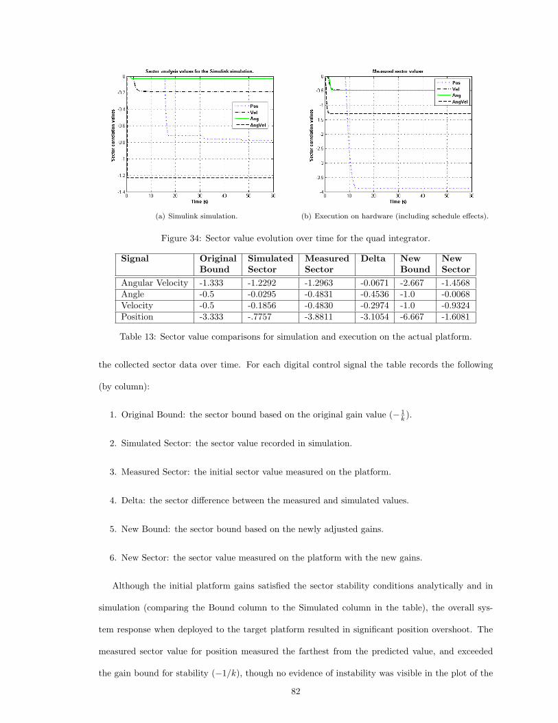
(a) Simulink simulation. (b) Execution on hardware (including schedule effects).
Figure 34: Sector value evolution over time for the quad integrator.
Signal Original Simulated Measured Delta New NewBound Sector Sector Bound Sector
Angular Velocity -1.333 -1.2292 -1.2963 -0.0671 -2.667 -1.4568Angle -0.5 -0.0295 -0.4831 -0.4536 -1.0 -0.0068Velocity -0.5 -0.1856 -0.4830 -0.2974 -1.0 -0.9324Position -3.333 -.7757 -3.8811 -3.1054 -6.667 -1.6081
Table 13: Sector value comparisons for simulation and execution on the actual platform.
the collected sector data over time. For each digital control signal the table records the following
(by column):
1. Original Bound: the sector bound based on the original gain value (− 1k ).
2. Simulated Sector: the sector value recorded in simulation.
3. Measured Sector: the initial sector value measured on the platform.
4. Delta: the sector difference between the measured and simulated values.
5. New Bound: the sector bound based on the newly adjusted gains.
6. New Sector: the sector value measured on the platform with the new gains.
Although the initial platform gains satisfied the sector stability conditions analytically and in
simulation (comparing the Bound column to the Simulated column in the table), the overall sys-
tem response when deployed to the target platform resulted in significant position overshoot. The
measured sector value for position measured the farthest from the predicted value, and exceeded
the gain bound for stability (−1/k), though no evidence of instability was visible in the plot of the
82

output trajectory. As all of the gains moved right up to the edge of their bounds when deployed,
we reduced all of the gains by 12 . Note that changing the gains changes the acceptable sector bound
as well as the actual sector bounds themselves (as shown in Table 13). After adjusting the gains all
of the sector values fell within the bounds.
On closer inspection we discovered that the most significant platform effect was a non-ideal
position gain condition for signals with frequencies too close to the sampling rate. Fig. 35 shows
a comparison of the ideal frequency response of the outer loop controller block with an empirically
measured frequency response for the same controller block deployed on the target hardware. Note
the spike at the right-hand side of the plot in Fig. 35(b). This is a nonlinear gain anomaly due to
the effects of the saturation block, and which appears only for signals with frequencies right near
the Nyquist sampling rate. The remedy was to add a simple input filter to cut off frequencies too
close to the sampling rate. This effectively slows down the possible commands that can be issued
to the system. The sector analysis blocks helped identify the position control component as the
element whose behavior was farthest from predicted when deployed to the platform. Adding a rate
limiter block to the reference input resolved the problem. Note that the full quadrotor model already
included a similar (but more complex) rate limiter.
(a) Analytically predicted response. (b) Measured response.
Figure 35: Magnitude frequency responses for the quad integrator.
The Quad Integrator model simulation exposed a few interesting and unanticipated defects in
our design, beyond the gain anomaly detected by the sector analysis. The most significant problem
was the asynchronous arrival of the input sensor data. Since the input data transfers were not
83

synchronized with the controller schedule, we had to add a double-buffer to the UART data handler
in order to eliminate data corruption.
Quadrotor Model
The final development phase integrated the full dynamics of the quadrotor, comprised of the full
data paths and nonlinear functions of the controllers. Figs. 36 - 38 show details from the full
Simulink model for the quadrotor. In the top-level design model (Fig. 36), the robo stix block
(Fig. 37) contains the functional specifications for the DataHandler (sensor convert block) and the
InnerLoop (inner loop block, also Fig. 38) software components. Likewise the gum stix block and
the ref data block specify functions for the OuterLoop and RefHandler software components.
Figure 36: Simulink model of the Starmac quadrotor helicopter.
We used the LogicPort probe to assess the correctness of the schedule. The configured schedule
(Fig. 39) correlates with the schedule points measured by the LogicPort analyzer for the tasks and
messages on the Robostix board (Fig. 40). Our experimental configuration did not provide a similar
means for accurate measurement of the timing on the Gumstix board, though we can observe that
message transfers start and end as predicted when task interference is absent. Task interference
84

Figure 37: Detail of the Robostix block.
was only observed for misconfigured schedules, or when other non-controller Gumstix processes
created heavy loads, delaying the controller. Both schedule-based and load-based interference were
eliminated for nominal operation. Fig. 41 illustrates tracking behavior for the xPC-simulated
Quadrotor, where the real-time controller implementation runs on the actual controller hardware.
The dashed curves represent the commanded x, y, and z positions as shown, and the solid lines show
the actual trajectory achieved by the HIL simulated helicopter using the deployed controller code.
Our first move to the full quadrotor model uncovered numerical problems with some of the emu-
lated floating-point functions provided by the gcc ARM cross-compiler. This forced us to implement
our own versions of the single-precision absolute value, signum, and minimum functions for the Out-
erLoop component. This problem was new to this phase of the evaluation because the rate limiter
was not present in the Quad Integrator model.
Lessons and Future Work
Probably the greatest difficulty in our work has been dealing with the large number of moving parts
involved in the development of the modeling language and tools, the modeling and implementation
85

Figure 38: Detail of the inner loop block.
of design examples, and the configuration of the development tools and execution environment for
the target platform. Our MIC-based solution only covered a part of the entire problem. We only
lightly addressed target system configuration, automated updates of the ESMoL model to track
changes in the Simulink design, and runtime assessment (of both the simulator for plant dynamics
and the target platform with the deployed code). We developed a technique for runtime assessment
of controller stability as covered in Porter et al[84] (described partially in the Quad Integrator
evaluation section), but it was difficult to automate due to the limited number of free data paths
available for debugging in our chosen target system. The integration of third party libraries in the
development of our tools, and variations in platform module behavior were not directly addressed
by our techniques, though they consumed significant development and testing time.
The next frontier in ESMoL development should be control loop modeling and analysis. Control
design formalisms abound, each with its own particular features and capabilities. Passivity and the
more general sector analysis formalisms are good examples of compositional frameworks which could
be encoded in modeling tools[86] and which could support incremental development.
86

Figure 39: Schedule configuration for the quadrotor.
Figure 40: Timing diagram for the Robostix AVR running the inner loop controller.
87

Figure 41: Trajectory tracking for the quadrotor implementation.
88

CHAPTER IV
INCREMENTAL SYNTACTIC ANALYSIS FOR COMPOSITIONAL MODELS:
ANALYZING CYCLES IN ESMOL
The ESMoL language is built on a platform which provides inherent correctness properties for
well-formed models. The properties include functional determinism, deadlock freedom, and timing
determinism. Establishing well-formedness for a particular model sometimes requires sophisticated
syntactic analysis of the global model structure. Where possible, for particular decomposable syn-
tactic analysis problems we would like to use the model structure to improve efficiency of analysis.
As design changes are made to the model, we would like to limit analysis to those components that
are affected by the modification.
Overview
Syntactic Analysis Challenges
One particular analysis problem concerns synchronous execution environments and system assembly.
In dataflow models of computation we are often concerned with so-called “algebraic” or delay-free
processing loops in a design. Many synchronous formalisms require the absence of delay-free loops in
order to guarantee deadlock freedom [87] or timing determinism [8]. This condition can be encoded
structurally into dataflow modeling languages – for example Simulink [88] analyzes for algebraic
loops and attempts to resolve them analytically. In the Ptolemy dataflow design environment,
such causality loops complicate scheduling requiring fixed-point iteration to ensure convergence of
results[89]. In this work we only consider the structural problem of loop detection in model-based
distributed embedded system designs.
Cycle Detection in ESMoL Models
We propose a simple incremental cycle detection technique with the following characteristics:
89

• The algorithm uses Johnson’s simple cycle enumeration algorithm as its core engine[90]. John-
son’s algorithm is known to be efficient[91]. We use cycle enumeration rather than simple
detection in order to provide useful feedback to the designers.
• The algorithm exploits the component structure of hierarchical dataflow models to allow the
cycle enumeration to scale up to larger models.
• A simple incremental interface is created and stored in each component as the analysis pro-
cesses the model hierarchy from the bottom up. The method should scale to large designs
without imposing onerous data storage requirements on the model, and allow highly efficient
recomputation of the cycle analysis when design changes occur in the model.
• The technique will not produce false positive cycle reports, though it may compress multiple
cycles into a single cycle through the abstraction. Fortunately, full cycles can be recovered
from the abstract cycles through application of the enumeration algorithm on a much smaller
graph.
Zhou and Lee presented an algebraic formalism for detecting causality cycles in dataflow graphs,
identifying particular ports that participate in a cycle. [52]. Our work traverses the entire model
and extracts all elementary cycles, reporting all ports and subsystems involved in the cycle. Our
approach is also inspired by work from Tripakis et al, which creates a richer incremental interface
for components to capture execution granularity as well as potential deadlock information[2]. Their
approach is lossless, in that it retains sufficient detail to faithfully represent dataflow structure and
execution granularity. It is much more complex in both model space and computation than our
approach. Our formalism does not aim to pull semantic information forward into the interface
beyond connectivity. In that sense our approach is more general, as it could be applied to multiple
model analysis problems in the embedded systems design domain.
The KPASSA model analysis tool described by Boucaron et al [92] performs task graph schedul-
ing analysis for latency-insensitive synchronous designs. Their formal model leans heavily on loop
structures, and as such one component of their tool relies on an implementation of Johnson’s cycle
90

enumeration algorithm[93]. Their formal model is specific to a particular model of computation,
and their application of cycle checking is only one small component of that solution.
Tools and Techniques
ESMoL Component Model
As the ESMoL language structure is documented elsewhere, we only cover details relevant to in-
cremental cycle checking. ESMoL is a graphical modeling language which allows designers to use
Simulink diagrams as synchronous software function specifications (where the execution of each block
is equivalent to a single bounded-time blocking C language call). These specifications are used to
create ESMoL component type blocks. ESMoL components have message structures as interfaces,
and the type specification includes a map between Simulink signal ports and the fields of the input
and output message structures.
Once software component types and interfaces have been specified, ESMoL designers instantiate
those components into a distributed deployment model. ESMoL allows the separate specification of
the logical data flow, the mapping of component instances to hardware, timing information for tasks
executing those components, and timing for messages sent over a time-triggered communication
bus. Code generated from the models conforms to an API for time-triggered execution. A portable
virtual machine implementation of the API allows execution in simulation, hardware-in-the-loop,
and fully deployed configurations[69].
ESMoL deliberately provides an unusual degree of freedom in creating software component types.
A designer can include Simulink references from any part of an imported dataflow model, and
instantiate them any number of times within the type definitions. The partition of functions into
ESMoL types allows the designer to control the granularity of functions assigned to distributed
tasks. Tasks can distribute functions over a time-triggered network for performance, or replicate
similar functions for fault mitigation. This level of flexibility requires automatic type-checking to
ensure compatibility for chosen configurations. Beyond interface type-checking, structural well-
formedness problems arise during assembly such as zero-delay cycles. Model analysis must ensure
well-formedness.
91

Cycle Enumeration
To implement cycle enumeration we use the algorithm Johnson proposed as an extension of Tiernan’s
algorithm [94] for enumerating elementary cycles in a directed graph[90]. Both approaches rely on
depth-first search with backtracking, but Johnson’s method marks vertices on elementary paths
already considered to eliminate fruitless searching, unmarking them only when a cycle is found.
Johnson’s algorithm is polynomial (O((n + e)c), where n, e, and c are the sizes of the vertex, edge,
and cycle set, respectively), and is still considered the best available general cycle enumeration
method[91]. We created an implementation of Johnson’s algorithm in C++ using the Boost Graph
library[95].
Hierarchical Graphs
For formally describing our incremental approach we use the algebra of hierarchical graphs intro-
duced by Bruni et al[96]. We repeat here their first definition: a design is a term of sort D generated
by
D ::= Lx[G] (10)
G ::= 0 | x | l < x >| G ‖ G | (νx)G | D < x >
Here term G represents a hierarchical directed graph, D is an edge-encapsulated hierarchical
graph, x is a vertex, x is a list of vertices in G (for which bxc is the corresponding set), l ∈ E (edge
labels of G, where edges can have n-ary connectivity ), Lx ∈ D (D are the design labels of G and x
are interface vertices in L), G ‖ G is parallel graph composition which merges vertices with common
names, (νx)G restricts the interface of graph G to exclude vertices in bxc, and the notation D < x >
maps the vertices from the interface of D to the vertices listed in x (renaming vertices internal to
the design for the external interface). Finally JGK indicates the graph corresponding to the term G.
Note that the term design is used for components in the hierarchy, each with a type and a set of
interface vertices. Unfortunately in the realm of graph theory the term component has a different
92

meaning. This algebraic model was conceived to more easily compute structural equivalence be-
tween hierarchical graphs. Bruni et al prove that syntactic equivalence between two design models
expressed as term algebras corresponds to isomorphism in their respective graphs[96] and conse-
quently equivalent behaviors in computational formalisms mapped to the algebras. Their formalism
also includes a definition of well-typedness, where types defined on the vertex set are only connected
if their types are compatible. Finally they define well-formedness for hierarchical graphs which in-
cludes well-typedness as a condition. We do not define the entire formalism here, only enough to
understand the essence of the connections between the terms and the graphs that they represent.
Incremental Cycle Analysis
Our intention is to support a design and analysis work flow that includes incremental analysis
steps. For example, a design may analyze part of the design before integrating it into a larger part
of the system. In our work flow, we envision storing the results of that first analysis along with
some interface data to reduce the cost of the second analysis. The same should hold true for the
system design. We should be able to analyze the system design efficiently, calculating incremental
analysis interfaces. When the system models are revised, whether by adding, removing, or modifying
components we can isolate the effects of the change on the cost of the analysis. Cycle analysis is a
useful example, but our aim is to tackle this problem more generally.
Formal Model
Let G be a well-formed hierarchical graph (as in Bruni [96]). To get more comfortable with the
notation, first note that graph G itself (without hierarchical structure) can be given as:
G = (‖ x) ‖ (‖(u,v)∈E l < u, v >) (11)
which is the parallel composition of the individual edge graphs of G, merged at their common
vertices.
Let C(G) be the set of elementary cycles in G, and let P (G, u, v) be the subgraph of G containing
all of the paths from vertex u to vertex v.
93

Consider a design of type W . Let W px [G] represent a parent design object in a graph hierarchy
with interface vertices x, and let W cixi
[G] be the design children of W p (JW ciK ⊂ JW pK). Then
neglecting vertex hiding and renaming to simplify the illustration, we have the following:
W px [G] = W p
x [(‖h xh) ‖ (‖(j,k) l < j, k >) ‖ (‖i W cixi
[G])] (12)
Eq. 12 describes the design W p in terms of its design children W ci , internal vertices xh, and
edges l < j, k >.
We introduce a new label lc into the sort for edges (E), which is used to connect vertices at
the boundaries of a design, abstracting the interface connectivity of the design. Introduce a new
mapping A : D → D′ from the designs of G to designs in a new graph G′. G′ is identical to G, but
adds the new edge label. This is the interface that we will use for incremental cycle analysis.
A(W cixi
[G]) =W cixi
[(‖h xh) ‖ (‖(j,k)∈bxic∧P (G,j,k) 6=∅ lc < j, k >) (13)
‖ (‖(j,k) l < j, k >) ‖ (‖m W cmxm
[G])])]
In this abstraction function the child designs are replaced by a much simpler connectivity graph.
We introduce two functions to support the algorithm:
R(A(W cix [G])) = W ci
xi[(‖x∈xi
x) ‖ (‖(j,k)∈lc lc < j, k >)] (14)
S(W px [G]) = W p
x [(‖h xh) ‖ (‖(j,k)∈bxc l < j, k >) ‖ (‖i R(A(W cixi
[G])))] (15)
R(·) and S(·) map designs in G to an abstracted design which only has connectivity edges for each
child design. In other words, when analyzing a component of G we use the incremental interface
data for each child component rather than its full details. This is a useful abstraction for cycle
detection: we can exploit the graph hierarchy to enumerate simple cycles more efficiently.
94

Algorithm Description
Assume we have a function FINDALLCYCLES : G → 2G which enumerates all elementary cycles in a
graph G, returning sets of subgraphs. Then Algorithm 1 adapts the general algorithm FINDALLCYCLES
to the hierarchical graph structure described above. We assume that G has a unique root design,
and that we have a function modified : D→ boolean which indicates whether a particular hierarchi-
cal component has been modified since the last run. New components in the model are considered
modified by default.
Algorithm 1 Hierarchical cycle detection1: cycles← []2: ifaces← {}3: function findhcycles( JW p
x [G]K )4: for all W ci
xi[G] ∈W p
x [G] do
5: FINDHCYCLES(JW cixi
[G]K)6: end for
7: modified(W px [G])← (modified(W p
x [G]) ∨ (∨cimodified(W cixi
[G]))8: if modified(W p
x [G]) then
9: T ← S(W px [G])
10: cycles← [cycles; FINDALLCYCLES(T )]11: ifaces[p]← A(T )12: end if
13: end function
14: FINDHCYCLES(G)
The algorithm performs a depth-first search on a hierarchical graph. If the component has been
modified, we compute connectivity interfaces for each subcomponent and check for cycles in the
parent component – the connectivity graph interface is substituted for each subcomponent. The
modification status is propagated up the hierarchy as the algorithm progresses. Each component
which has a modified child will also be marked as modified. The cycles are accumulated as the
algorithm ascends to the top of the model.
The runtime for the extended algorithm is slightly worse than Johnson’s algorithm in the worst
case, as it must also compute the interface graphs. In the average case the cycle checking proceeds
on graphs much smaller than the global graph, offsetting the cost of finding paths in each subgraph.
Further, if the incremental interface edges are stored in the model following the analysis, then
95

scalability is enhanced when incrementally adding functions to a design. Cycle analysis is then
restricted to the size of the new components together with the stored interfaces.
ESMoL Language Mapping
Now to map ESMoL logical architecture models onto this cycle-checking formal model we use the
following rules:
Subsys ::= LSubsysi,o
JDataflowK
Dataflow ::= 0 | x | lD < x > | Subsys < x, x >
| Dataflow ‖ Dataflow | (νx)Dataflow
MsgType ::= Me,eext (16)
SysTypeDef ::= Subsys < i, o > | lS < x, x >
| SysTypeDef ‖ SysTypeDef |MsgType < x, y >
SysType ::= LSysyi,yo
J(νx)(νe)SysTypeDefK
LogicalModel ::= SysType < i, o > | lL < o, i >
| LogicalModel ‖ LogicalModel
Briefly (from the bottom rule to the top), logical models consist of component blocks (SysType)
whose interface ports connected by edges. Component blocks are specified by Simulink dataflow
blocks (Dataflow) whose interface ports are connected either to other Simulink dataflow blocks or
to fields in message instances. Each message instance (MsgType) inside a system component type
block also has an interface vertex (y) which faces outward, and all other vertices are hidden within
the component (νx)(νy)SysTypeDef . At the logical architecture model level, data is exchanged via
messages which aggregate the individual dataflow connections within the components. Dataflow
blocks are built up from connections between functional vertices and between the interfaces on
composite subsystem blocks (Subsys). These each correspond to sorts in the ESMoL term algebra.
96

Let i, o, and e be vertex sorts corresponding to input ports, output ports, and message elements
respectively. Let s, c, f , and d be edge sorts (of lD, above) representing signal edges, connectivity
edges (as described above to support the incremental interface), f for Simulink primitive function
blocks, and d for delay blocks. The f function edge sorts are n-ary, so each function block can have
an arbitrary but finite number of input and output connections. For lS define the sorts (given with
their interfaces) lb,b < o, i >, lm,b < e, i >, and lb,m < o, e >. These represent the three different
connection types in a SysType specification, for connecting between ports of Simulink blocks (from
outputs to inputs) (lb,b), from message elements to Simulink input ports (lm,b), and from Simulink
output ports to message elements (lb,m).
Finally we give an encoding of terms representing ESMoL models into the more general hierar-
chical graph algebra:
x = x
LSubsysi,o
JDataflowK < x, x > = LxJGK < x >
Me,eextJK < x, y > = LxJGK < x >
LSysi,o
J(νx)(νe)SysTypeDefK = LyJGK < x > (17)
lD < x > = l < x >
l∗ < x, x > = l < x >
(νx)Dataflow = (νx)G
The encoding assigns the various layers of hierarchy from the ESMoL component type system to
hierarchical designs in the graph. Edges from all layers map to (possibly generalized) edges in the
new graph, and ports map to vertices.
The final piece is the application to finding delay-free loops. For a given ESMoL model, simply
remove all delay edges (sort elements d). Then invoke the algorithm. For the results, if a cycle
is found in a component we can construct a more detailed cycle model by substituting paths from
the connectivity edge sort with their more detailed equivalents in the descendants of the component
97

(recursively descending downwards until we run out of cycle elements). Call this subgraph the
expanded cycle. Repeating the cycle enumeration algorithm on these structures should yield the full
set of elementary cycles, and still retain considerable efficiency as we are only analyzing cycles with
possible subcycles, which can be a relatively small slice of the design graph.
Evaluation
Fixed-Wing Aircraft Example
Figure 42: Simulink Fixed Wing Controller Model
Our case study covers cycle analysis of the control design for a fixed-wing aircraft. The Simulink
model (Fig. 42) shows the four controller blocks and the sensor data handler. The particulars
of the control architecture are not important for this example, but Kottenstette covers them in
detail[97]. The controller has five software functions which are specified as Simulink model blocks,
and a dynamics component (the Cessna plant block). The MDL2MGA model importer creates
a structural replica of the Simulink model in the ESMoL modeling language. We use subsystems
from the replica to specify the function of synchronous software components. Fig. 43 illustrates
one possible configuration of the fixed wing controller components. In this particular configuration
(Fig. 43) the entire dataflow is included in one type definition, which means that the entire system
98

Figure 43: Synchronous data flow for Fixed Wing Controller
will execute together as a single synchronous function with all blocks firing at the same rate. This
particular configuration is useful for illustration, but is not the most practical implementation choice.
Incremental Analysis Results
Table 14 contains data from the analysis of the fixed wing model. The first pass was performed
incrementally, with each subcomponent of the top level model analyzed first. Then the top level
is analyzed using the stored path edges in the lower models. The table reports two run times
for the analysis of each component – the first is the processing time required to find the abstract
cycles only, and the second is the full analysis which finds the expanded cycle for each abstract
cycle (enumerating possibly multiple cycles per abstract cycle). The table also displays the number
of hierarchical components visited and the number of individual model elements visited, together
with the number of abstract cycles found and the total number of cycles. The table row labeled
top level (incremental) contains the results for the analysis of the top level of the model once the
individual path interfaces had been created for each of its subcomponents. The second pass (labeled
top level (full)) analyzed the entire fixed wing model at once, reporting the same quantities. Our
assessment of the scalability of the approach is inconclusive for three reasons – 1) the model size is
99

moderate, so overhead is likely large enough to be a significant factor in all of the run times, 2) we
would need a comparison with time taken to process a fully flattened model, including the flattening
traversals, and 3) we need to find larger models for our test set. The analyzer found 18 abstract
cycles and 54 detailed cycles at the top level for both passes. The velocity controller component also
contained a single abstract cycle (consisting of two detailed cycles). Note that we analyzed for all
cycles rather than only delay-free cycles to assess scalability. Total runtime was roughly equivalent
between the full and incremental methods for this particular model. The results so far are promising
but inconclusive as far as improved performance.
Abstract Full Abstract TotalComponent Run Run Hier. Total Cycles Cycles
Time (s) Time (s) Comps. Elts. Found Foundalpha beta mu controller 0.9 0.9 9 80 0 0gamma chi controller 1.6 1.6 7 134 0 0gamma chi mu sensor 1.3 1.3 8 100 0 0omega controller 0.9 0.9 9 80 0 0velocity controller 0.6 0.8 6 60 1 2Top level (incremental) 2.3 55.1 1 21 18 54Totals 7.6 60.6 19 872
Top level (full) 7.9 60.5 42 554 19 56
Table 14: Cycle analysis comparisons for the fixed wing model.
Figs. 44 and 45 display a subset of the velocity controller component which contains a cycle,
along with the expanded cycle for the component, in order to illustrate the cycle refinement in
greater detail. The abstract cycle search discovered the presence of a cycle within the component,
but part of the cycle lies within a subcomponent (anti windup control). The cycle detection for
anti windup control created a single path edge in the interface between the In1 port and the Out2
port, which corresponds to two paths within anti windup control. The full cycle as shown (Fig. 45)
is constructed in the analyzer, and then one more pass of Johnson’s algorithm resolves the two cycles
within the full cycle graph as reported in Tab. 14. The extracted cycle graph is much smaller (13
elements) than the corresponding fully flattened velocity controller model, which would contain 60
elements.
100

Figure 44: Detail of the components involved in the cycle found in the velocity controller.
Future Work
The current implementation is integrated into the ESMoL tool suite for the Generic Modeling
Environment[71], but thorough scalability testing requires larger models.
One interesting observation is the generality of the approach. Algorithm 1 very nearly captures
a generic procedure for bottom-up incremental syntactic analysis of hierarchical graphical models.
Algorithm 2 proposes such a generic template. A complete study of such generic structural analysis
techniques should include consideration of the effects of the component processing order on the
accuracy of the result.
101

Algorithm 2 Hierarchical cycle detection1: results← []2: ifaces← {}3: function analyze( JW p
x [G]K )4: for all W ci
xi[G] ∈W p
x [G] do
5: ANALYZE(JW cixi
[G]K)6: end for
7: modified(W px [G])← (modified(W p
x [G]) ∨ (∨cimodified(W cixi
[G]))8: if modified(W p
x [G]) then
9: T ← ANALYZESTRUCTURE(W px [G])
10: results← [results; COLLECTRESULTS(T )]11: ifaces[p]← CREATEINTERFACE(T )12: end if
13: end function
14: ANALYZE(G)
Two immediate applications of this generic incremental method in ESMoL embedded control
system designs are 1) automated sector analysis for passivity and/or stability and 2) quantization
interval analysis for data precision and overflow. Both represent a static analysis of possible system
behaviors that can be encoded syntactically. In both cases component interface data requirements
are small, and computation is fairly efficient.
102

Figure 45: Full cycle for the velocity controller.
103

CHAPTER V
INCREMENTAL TASK GRAPH SCHEDULE CALCULATION
Analysis of semantic correctness properties depends on formal representations of the system be-
haviors represented by the model. The difficulty with semantic analysis is that concurrent behaviors
over time may not correlate well with the structure of the model, since a proper behavior model
will capture the numerous interactions between components and their effects on seemingly unrelated
components. Semantic analysis is usually more computationally expensive than syntactic analyses,
because of the need to look at states of the model over time. As discussed previously, incremental
techniques may provide efficient analysis if they do not introduce behavioral approximations which
are too conservative. The difficulty lies in finding useful decompositions of behavioral abstractions
which will allow incremental analysis.
Overview
Semantic Analysis Challenges
A well-formed ESMoL model represents a particular set of system behaviors. Prior to schedule
calculation the set of possible behaviors is underdetermined, leading to phenomenally large numbers
of possible schedule configurations, many of which are essentially equivalent from the point of view of
the requirements. ESMoL requires a scheduling technique which can use the timing and dependency
information in the model to create a valid configuration for the execution of tasks and messages in the
time-triggered network. Of particular concern is the satisfaction of end-to-end latency constraints
for scheduled task graphs. Many scheduling techniques support offsets and local deadlines to support
specified dependencies, but do not specify how those offsets and deadlines should be determined.
We need a scalable schedule calculation tool which supports iterative rework of design components
and round-trip integration of the scheduling tool in the design flow.
104

Schedule Analysis and Calculation
We present here a conceptual design for an incremental scheduling and allocation algorithm which
addresses the problems of scalability by incrementally computing task schedules for additional la-
tency constraints. Specifically we propose a modification of the Bubble Scheduling and Allocation
(BSA) algorithm[98] to handle node-locked tasks and incremental addition of new tasks, network
data communication, and latency requirements.
Tools and Techniques
Task Graph Scheduling and Abstractions
Kwok and Ahmad present a detailed evaluation and comparison of many task graph scheduling
techniques[33]. We will rely on their description of the task graph scheduling problem, and describe
a few of the useful scheduling abstractions that are common to some of the algorithms. We are
most interested in the Arbitrary Processor Network (APN) class of scheduling algorithms, which
assign tasks to processors and start times to tasks in a particular network topology. A task graph
is a directed acyclic graph (DAG) G = (V,E), where vertices correspond to computational tasks
having a known, bounded execution time, and edges correspond to messages transferred over a
communication network. Vertices having no inbound edges are denoted entry vertices or sources,
and vertices having no outbound edges are denoted exit vertices or sinks. Each vertex and edge has
a set of weights, corresponding to the computation time required to execute the task represented
by the node or to transfer the message represented by the edge. These execution times may differ
for each processor or network link, so task and message weights are given as functions of vertex and
processor (or edge and network). Let w(ni, Pk) be the task computation cost (execution time) for
vertex vi on processor Pk. Likewise let c(vi, vj , Nl) be the cost (transfer time) for the message from
vertex vi to vertex vj over network link Nl. If two task vertices are scheduled on the same processor,
then the communication cost of an edge between them is counted as zero. The vertex and edge
weights may be determined by estimation, measurement, or static analysis. For schedule analysis
they should be considered bounds on worst-case execution time rather than nominal values.
105

The b-level (bottom-level) of a task vertex measures the longest path from the vertex to an exit
vertex, counting both vertex execution time and data transfer times on the network. The t-level
(top level) measures the longest path distance from an entry vertex to the vertex in question, not
including its own weight. These levels are frequently used in scheduling heuristics to assign priorities
to tasks during scheduling. The t-level roughly represents the earliest start time for a vertex in the
DAG. A critical path (CP) is the longest path from a particular entry vertex to an exit vertex. In
most of the literature the critical path is abstracted as the longest possible path in the task graph,
bounding the b-level values for that graph. For our purposes the task graphs may have multiple
critical paths, where each corresponds to a latency requirement. More formally, given a task DAG G,
latency requirements can be specified as triples Lm = (vi, vo, tm). Here vi indicates a source vertex,
vo indicates a sink vertex, and tm indicates a time requirement within which all paths between vi
and vo must execute. Then CPm represents the critical path from vi to vo for requirement Lm.
Bubble Scheduling and Allocation (BSA)
The Bubble Scheduling and Allocation (BSA) Algorithm[98] first determines a critical path in the
task graph by considering the b-level and t-level of task vertices. The CP determines a partition
of the graph into IB (in-branch) vertices, CP (critical path) vertices, and NA vertices, which are
successors to other kinds of vertices, originally called out-branch vertices in [98]. We slightly adjust
the b-level so that NA vertices have a value blevel(v) = 0, CP vertices start with blevel(vo) = 1, and
all predecessor b-level values are determined as described. Then the critical path and its in-branch
vertices (IBVs) are scheduled serially to a single processor (the pivot processor) using the routine
SERIALINJECT. The function SERIALINJECT places all of the task graph vertices into descending b-
level order. This is a slightly different presentation from the original description in Kwok[98], but
it satisfies all of the precedence dependencies for each vertex in the critical path as required by the
BSA algorithm. Our slightly modified b-level calculation also ensures that NA vertices are scheduled
after latency-critical tasks.
The BSA algorithm (Algorithm 3) proceeds by iterating over the system processors (starting
with the initial pivot processor) and testing scheduled vertices for migration. If a tested vertex
106

could start earlier on another processor, or if moving the vertex will reduce network data transfers
without impacting the overall length of the critical path then the algorithm migrates the tested task.
We assume that all times are discretized, and thus given as integer values. Table 15 describes the
critical functions, routines, and variables. Some of the algorithmic functions are not fully defined
here to save space.
Function orRoutine DescriptionSERIALINJECT Sequences the vertices in decreasing order of blevel, scheduling them
to the specified processor.SCHED Starts from a migrated vertex, calculating start times for it and all
successive vertices based on their processor assignment.SORTPROCS Orders the processors in the system according to a weighting function
based on available space and cost-based proximity to the processors towhich the start and end vertex are bound.
FINDCRITICALPATH Calculates the b-levels of the specified vertices with respect to theentry and exit, and marks the CP and IB vertices.
CALCSTART Finds the best start time for a particular task vertex on the specifiedprocessor, subject to data dependencies.
Variable Descriptionstart Array mapping vertices to their currently configured start times.finish Array mapping vertices to their currently configured end times.dat The earliest time at which a vertex could be scheduled, based on
the arrival times of its data dependencies.vip For a given vertex, the immediate vertex predecessor whose data
arrives last.proc Array mapping vertices to their currently assigned processor.proclist A priority-sorted list of processors.pivot The current processor.
Table 15: Function and variable definitions.
107

Algorithm 3 BSA Algorithm1: start← {(n0, 0), (n1, 0), . . . , (ninf , 0)}2: finish← {(n0, 0), (n1, 0), . . . , (ninf , 0)}3: dat← {(n0, 0), (n1, 0), . . . , (ninf , 0)}4: vip← {(n0, n0), (n1, n0), . . . , (ninf , n0)}5: function bsa(G,H)6: proclist← SORTPROCS(H)7: pivot← proclist[1]8: CP ← FINDCRITICALPATH(G)9: proc← SERIALINJECT(pivot, G, CP, H)
10: for all idx ∈ [1, len(proclist)] do
11: pivot← proclist[idx]12: for all n ∈ {n|proc(n) = pivot} do
13: BestFT ← 014: BestProc← pivot
15: if start(n, pivot) > dat(n, pivot) ∨ proc(vip(n)) 6= pivot then
16: for all p ∈ adj(pivot) do
17: FT ← CALCSTART(n, p) + w(n, p)18: if FT < finish(n, pivot) ∨ (FT = finish(n, pivot) ∧ proc(vip(n)) = p) then
19: BestFT ← FT
20: BestProc← p
21: end if
22: end for
23: if p 6= pivot then
24: proc(n)← p
25: SCHED(G, H, proc, n)26: end if
27: end if
28: end for
29: end for
30: end function
The rationale for the BSA algorithm is as follows. The authors assume that local data transfers
are zero-cost, so the best starting point for the schedule should have the least message transfers.
Accordingly, SERIALINJECT places all of the vertices on a single processor. All improvements beyond
the serial configuration come from moving vertices to adjacent processors where they can start early
enough to “hide” the network data transfer cost. As iteration proceeds down the critical path, the
migration process reduces the overall potential schedule length with each move of a vertex. The
BSA algorithm can be adapted to handle non-uniform data transfers (i.e. different transfer times
for different routes) in the calculation of start times for adjacent processing nodes. As the authors
108

suggest, using the task finish time in the adjacent processor comparisons also adapts the algorithm to
a heterogeneous network with processors running at different speeds[98]. Once the CP and all of its
input dependencies (CP and IB vertices) have been scheduled, the remaining vertices (marked NA)
can be scheduled anywhere convenient in order to reduce network usage or satisfy other objectives.
Incremental Schedule Analysis
We will add a few more problem constraints and assumptions appropriate to our incremental variant
of the task graph problem, and adapt the BSA algorithm to meet them:
1. In a real-time system particular tasks are bound to specific processors due to I/O require-
ments. We will assume that the starting and ending vertex of each critical path correspond
to processor-locked tasks. The problem input will include the assignments for those particular
processors.
2. We assume that an existing schedule has already been placed on the network, and that
the next task graph contains only a single critical path. The pre-existing schedule tasks
are tagged for each critical path in which they participate. For each latency requirement
(Lm corresponding to a single critical path CPm), any vertex is either critical (CP), an
in-branch dependency (IB), or neither (NA). The resulting vertex list has the form vi :
{(CP1, CP ), (CP2, IB), (CP3, NA), . . .}.
3. Any new task graph to be added to the schedule may use existing tasks as part of its speci-
fication. We refer to the shared vertices as merge vertices. However, those composed graphs
may not form a cycle. The full graph is still a DAG with (possibly) multiple input and output
vertices.
4. At the start of the algorithm we have a slack value for each CP in the pre-existing DAG,
which represents an amount by which each CP could expand without violating its end-to-end
deadline.
109

Concepts
The supported work flow for this algorithm proceeds by scheduling the tasks corresponding to
individual requirements sequentially, incrementally adding a DAG with a new CP at each stage
as described below. The critical insights are that the initial pre-existing schedule is packed down
towards the entry tasks, so any flexibility in the schedule will come from expanding those graphs
towards the end of the schedule within the specified slack. That takes a particular form in our
approach. If we consider merging two critical paths at specified vertices, then either they are 1)
disjoint, 2) meet at a single vertex, 3) meet at sequential vertices (i.e. they share a single common
path), or 4) they meet at multiple non-sequential vertices. Case 4 can create problems for our
incremental approach. If the CPs meet at multiple non-sequential vertices, then two or more paths
exist between each pair. As those multiple paths are shared by both CPs, we may have modified
either critical path with a longer segment. This is handled by identifying merge vertices which
create multiple paths between CPs. If the path segment from the new CP is longer, then we use
slack to expand the schedule distance between those vertices (by moving back the later vertex in the
pair). We allow the existing CPs to expand beyond their available slack, but during scheduling all
expanded CPs must be packed back down to within their original deadline (positive slack). Once all
of the multi-path pairs are expanded towards the end of the schedule, the BSA-style optimization
to pack the extra slack back down towards the beginning can proceed.
In BSA, placement of the entry vertex of the new CP is critical, because the BSA algorithm does
not ever move the entry vertex in the schedule. Obviously, if the new CP includes existing vertices,
then a poor scheduling choice for the initial vertex can cause an infeasible or unnecessarily long
schedule. The first segment of the new CP (from the entry vertex to the first merge vertex) will not
pack down, because the first merge point is already “packed”. Our solution is to place the entry
vertex at the start of the earliest empty segment where the serial injection procedure will reach the
merge vertex. Then we use a reverse-BSA algorithm down from the first merge vertex to pack the
start of the new CP forward, and use the forward-BSA algorithm to pack the remaining vertices
backwards, consuming slack that was given during the initial expansion.
110

Algorithm Definition
Assume we are given the following inputs, assumptions, and definitions:
• Existing schedule: Given a network topology H, an original weighted task graph G, a
schedule of start times defined on the vertices of G (start : V (G)→ Z), processor assignments
for all of the vertices of G (proc : V (G) → [1, P ]), a set of latency requirements (Lm,m ∈
[1,M ]), a collection of tags for the vertices (one for each vertex for each requirement) (tag :
V (G) ×M → {CP, IB, NA}|V (G|), and a set of slacks for each latency requirement ( slack :
M → Z ),
• New task graph: Given a new weighted task graph G′, with latency requirement Lm+1 and
corresponding critical path CP’. We also have processor assignments for the entry and exit
vertices of CP’ (proc : vi, vf → [1, P ]).
• Assume that G ∪G′ is cycle-free.
• Let Vs and Es represent the shared vertices and edges of G ∩G′.
• A vertex v is a pure free vertex if tag(v) = {(l, NA)| ∀l ∈ [1,M ]}. Denote this set pfv(G).
• Consider (G ∪ G′) − pfv(G ∪ G′). Scheduling excludes pure free vertices in order to obtain
maximum scheduling freedom, as all significant (i.e. IB and CP) vertices should be involved
in one or more of the critical paths.
111

Algorithm 4 Incremental BSA Setup1: function ibsasetup(G,G′,H,start,proc,tag,slack)2: CDS ← SERIALINJECT(dummy, G′, CP ′, H)3: pairs← FINDFORKS(G, G′, CDS)4: for all (v1, v2, cp) ∈ pairs do
5: Let v1,n = v|v ∈ CDS ∧ (v1, v) ∈ E′.6: Let v2,p = v|v ∈ CDS ∧ (v, v2) ∈ E′.7: Let cost = c(v1, v1,n) +
∑v∈CDS,v∈path(v1,v2)
w(v) + c(v2,p, v2).8: Let dist = start(v2, proc(v2)− start(v1, proc(v1)).9: start(v2, proc(v2)) = start(v2, proc(v2)) + (cost− dist)
10: SCHED(G, H, proc, v2)11: slack(cp)← slack(cp)− (cost− dist)12: end for
13: Let v = v1|(v1, v2) ∈ pairs[1]14: return v
15: end function
The setup for the incremental BSA algorithm (Algorithm 4) performs the following steps:
• Determination of an initial sequence for G′, using a dummy processor with no preexisting task
vertices (line 2).
• Calculating the paired vertices of CP’ which result in multiple branches when merged with the
preexisting CPs (line 3).
• For each pair (v1, v2) and associated preexisting CP (indexed by the integer cp in the algo-
rithm):
– Find the first vertex after v1 in CP’ (line 5).
– Find the last vertex before v2 in CP’ (line 6).
– Calculate the cost of the newly added segment from CP’ (line 7).
– Compare the new segment cost with the distance (dist) from v1 to v2 in the current
schedule, and the slack for CP. (line 9).
– If the move is acceptable, move back v2 by cost− dist, and reschedule the vertices of CP
from that point.
• Return the first vertex of the first pair for splitting the scheduling of CP’ into forward and
reverse segments (line 14-15).
112
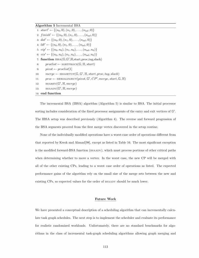
Algorithm 5 Incremental BSA1: start′ ← {(n0, 0), (n1, 0), . . . , (ninf , 0)}2: finish′ ← {(n0, 0), (n1, 0), . . . , (ninf , 0)}3: dat′ ← {(n0, 0), (n1, 0), . . . , (ninf , 0)}4: ldt′ ← {(n0, 0), (n1, 0), . . . , (ninf , 0)}5: vip′ ← {(n0, n0), (n1, n0), . . . , (ninf , n0)}6: vis′ ← {(n0, n0), (n1, n0), . . . , (ninf , n0)}7: function ibsa(G,G′,H,start,proc,tag,slack)8: proclist← SORTPROCS(G, H, start)9: pivot← proclist[1]
10: merge← IBSASETUP(G, G′, H, start, proc, tag, slack)11: proc← ISERIALINJECT(pivot, G′, CP ′,merge, start, G, H)12: BSAREV(G′, H,merge)13: BSAADV(G′, H,merge)14: end function
The incremental BSA (IBSA) algorithm (Algorithm 5) is similar to BSA. The initial processor
sorting includes consideration of the fixed processor assignments of the entry and exit vertices of G′.
The IBSA setup was described previously (Algorithm 4). The reverse and forward progression of
the BSA segments proceed from the first merge vertex discovered in the setup routine.
None of the individually modified operations have a worst-case order of operations different from
that reported by Kwok and Ahmad[98], except as listed in Table 16. The most significant exception
is the modified forward-BSA function (BSAADV), which must process portions of other critical paths
when determining whether to move a vertex. In the worst case, the new CP will be merged with
all of the other existing CPs, leading to a worst case order of operations as listed. The expected
performance gains of the algorithm rely on the small size of the merge sets between the new and
existing CPs, so expected values for the order of BSAADV should be much lower.
Future Work
We have presented a conceptual description of a scheduling algorithm that can incrementally calcu-
late task graph schedules. The next step is to implement the scheduler and evaluate its performance
for realistic randomized workloads. Unfortunately, there are no standard benchmarks for algo-
rithms in the class of incremental task-graph scheduling algorithms allowing graph merging and
113

Function or Order ofRoutine Description OperationsFINDFORKS Walk the new CP, finding vertex pairs that cause
forks in the merged paths, and their original CP. O(em)SORTPROCS Sort the processors according to available time. O(pv)ISERIALINJECT Perform SERIALINJECT with a few changes: find
the start of the first empty space prior to merge, and aswe move forward, skip over existing vertices. Put allof the NA nodes back into the schedule. O(e + v)
BSAREV Perform BSA backward from merge. O(p2ev)BSAADV Perform BSA forward from merge, checking CP
dependencies for merged CP-nodes before moving them. O(p2evm)Variable Descriptionldt The latest time at which a particular vertex could be scheduled,
based on the required send times of its successors.vis For a given vertex, the immediate vertex successor whose data
must arrive first.
Table 16: Function and variable definitions for incremental BSA.
task-processor binding. Some of the random benchmark graphs described by Kwok and Ahmad
could be adapted for this evaluation[33]. The overall schedule length metric is also not wholly ap-
propriate for comparison, unless we consider only the improvement of each latest addition to the
schedule.
The scheduler is intended as a replacement for the scheduling analysis algorithm for the ESMoL
language originally proposed in Porter et al[70]. The original scheduler created feasible schedules,
but had difficulty enforcing end-to-end latency constraints consistently. This scheduler includes
allocation and scheduling, which makes the integration prospects more interesting for ESMoL. The
next step is integration with the ESMoL scheduling specification language.
If necessary to improve scalability, we should consider encoding some of the useful task graph
scheduling abstractions as constraint problems. Earlier work in constraint programming for schedule
calculation shows that constraint-based techniques scale very well to large problems with many
dependencies [34][70]. BSA is essentially a search over multiple dimensions, with interval narrowing
of the start times towards the beginning of the schedule. It should be possible to investigate this
approach to see if it can yield a more scalable version of the algorithm.
114

CHAPTER VI
CONCLUSIONS: WHAT HAVE WE LEARNED?
The ESMoL language and tools provide sufficient expressiveness and detail to analyze and gener-
ate functional quadrotor control software for deployment on a time-triggered distributed processing
network. The reach of our model-integrated tool environment was not sufficient to capture all of
the difficult details involved in our modeling example, so further work on library integration for tool
development and runtime evaluation are particularly important.
Model structure can facilitate the specification and implementation of incremental syntactic
model analysis. Our example offers a proof of concept, and the expectation that where system be-
havior can be represented compositionally according to the hierarchical structure of the model, such
techniques will prove beneficial. Further work will determine scalability of our analysis approach,
though conceptually the incremental approach already increases the flexibility of the development
process.
For purely semantic properties, a proper choice of behavioral abstractions can permit incremental
analysis as well. Our scheduling approach is only conceptual, but illustrates the richness of this line
of inquiry. Further work will implement and evaluate this potentially useful technique, in order to
assess scalability of the algorithm and conservatism of the results produced by it.
115
BIBLIOGRAPHY
[1] I. Shin, “Compositional framework for real-time embedded systems,” Ph.D. dissertation, Univ.
of Pennsylvania, Philadelphia, 2006.
[2] S. Tripakis, D. Bui, M. Geilen, B. Rodiers, and E. A. Lee, “Compositionality in Synchronous
Data Flow: Modular Code Generation from Hierarchical SDF Graphs,” Univ. of California,
Berkeley, Tech. Rep. UCB/EECS-2010-52, 2010.
[3] T. Henzinger and J. Sifakis, “The embedded systems design challenge,” in FM: Formal Methods,
ser. LNCS 4085. Springer, 2006, pp. 1–15.
[4] S. McConnell, Rapid Development: Taming Wild Software Schedules. Redmond, WA: Microsoft
Press, 1996.
[5] G. Karsai, J. Sztipanovits, A. Ledeczi, and T. Bapty, “Model-integrated development of em-
bedded software,” Proc. of the IEEE, vol. 91, no. 1, pp. 145–164, Jan 2003.
[6] E. K. Jackson and J. Sztipanovits, “Towards a formal foundation for domain specific modeling
languages,” Proc. of the Sixth ACM Intl. Conf. on Embedded Software (EMSOFT’06), pp.
53–62, Oct 2006.
[7] H. Kopetz and G. Bauer, “The time-triggered architecture,” Proc. of the IEEE, Special
Issue on Modeling and Design of Embedded Software, Oct 2001. [Online]. Available:
citeseer.ist.psu.edu/kopetz88timetriggered.html
[8] E. A. Lee and D. G. Messerschmitt, “Synchronous data flow,” Proc. of the IEEE, vol. 75, no. 9,
pp. 1235–1245, 1987.
[9] J. T. Buck, “Scheduling Dynamic Dataflow Graphs with Bounded Memory Using the Token
Flow Model,” Ph.D. dissertation, Univ. of California, Berkeley, 1993.
[10] A. Fettweis, “Wave digital filters: theory and practice,” Proc. of the IEEE, vol. 74, no. 2, pp.
270 – 327, 1986.
[11] N. Kottenstette, J. Hall, X. Koutsoukos, P. Antsaklis, and J. Sztipanovits, “Digital control of
multiple discrete passive plants over networks,” Intl. Journal of Systems, Control and Com-
munications (IJSCC), no. Special Issue on Progress in Networked Control Systems, 2009, to
Appear.
[12] N. Kottenstette, H. LeBlanc, E. Eyisi, and X. Koutsoukos, “Multi-rate networked control of
conic systems,” Sep 2009.
[13] G. Niemeyer and J.-J. E. Slotine, “Stable adaptive teleoperation,” IEEE Journal of Oceano-
graphic Engineering, vol. 16, pp. 152–162, 1991.
[14] John Hudak and Peter Feiler, “Developing AADL Models for Control Systems: A Practitioner’s
Guide,” CMU SEI, Tech. Rep. CMU/SEI-2007-TR-014, 2007.
116

[15] F. Singhoff, J. Legrand, L. Nana, and L. Marce, “Scheduling and memory requirements analysis
with AADL,” Ada Lett., vol. XXV, no. 4, pp. 1–10, 2005.
[16] “The Cheddar project : A free real time scheduling analyzer,” http://beru.univ-
brest.fr/ singhoff/cheddar.
[17] T. Henzinger, B. Horowitz, and C. Kirsch, “Giotto: A time-triggered language for embedded
programming,” Proc. of the IEEE, vol. 91, pp. 84–99, Jan 2003. [Online]. Available:
http://www.gigascale.org/pubs/397.html
[18] E. Farcas, C. Farcas, W. Pree, and J. Templ, “Transparent distribution of real-time components
based on logical execution time,” in Proc. of the 2005 ACM Conf. on Lang., Compilers, and
Tools for Embedded Systems (LCTES ’05). New York, NY: ACM Press, Jun 2005, pp. 31–39.
[19] A. Naderlinger, J. Pletzer, W. Pree, and J. Templ, “Model-Driven Development of FlexRay-
Based Systems with the Timing Definition Language (TDL),” in Proc. of the 4th Intl. ICSE
workshop on Software Eng. for Automotive Systems, Minneapolis, May 2007.
[20] F. Balarin, Y. Watanabe, H. Hsieh, L. Lavagno, C. Paserone, and A. L. Sangiovanni-Vincentelli,
“Metropolis: an integrated electronic system design environment,” IEEE Computer, vol. 36,
no. 4, Apr 2003.
[21] N. Pontisso and D. Chemouil, “Topcased combining formal methods with model-driven engi-
neering,” in ASE ’06: Proc. of the 21st IEEE/ACM International Conf. on Automated Software
Engineering. Washington, DC, USA: IEEE Computer Society, 2006, pp. 359–360.
[22] S. Tripakis, C. Sofronis, P. Caspi, and A. Curic, “Translating discrete-time simulink to lustre,”
ACM Trans. Embed. Comput. Syst., vol. 4, no. 4, pp. 779–818, 2005.
[23] D. Park, Innovations and Advanced Techniques in Computer and Information Sciences and
Engineering. Springer Netherlands, 2007, ch. Translation of Safety-Critical Software Require-
ments Specification to Lustre, pp. 157–162.
[24] R. Alur and G. Weiss, “RTComposer: a framework for real-time components with scheduling
interfaces,” in EMSOFT ’08: Proc. of the 8th ACM Intl. Conf. on Embedded software. New
York, NY, USA: ACM, 2008, pp. 159–168.
[25] W. Herzner and R. S. et al, “Model-Based Development of Distributed Embedded Real-Time
Systems with the DECOS Tool-Chain,” in Proc. of SAE 2007 AeroTech Congress & Exhibition,
Los Angeles, CA, USA, Sep 2007.
[26] S. Edwards, L. Lavagno, E. A. Lee, and A. Sangiovanni-Vincentelli, “Design of embedded
systems: Formal models, validation, and synthesis,” Proc. of the IEEE, vol. 85, no. 3, pp.
366–390, Mar 1997.
[27] A. Easwaran, “Advances in hierarchical real-time systems: Incrementality, optimality, and mul-
tiprocessor clustering,” Ph.D. dissertation, Univ. of Pennsylvania, 2008.
117

[28] E. Wandeler, “Modular performance analysis and interface-based design for embedded real-time
systems,” Ph.D. dissertation, Computer Engineering and Networks Laboratory, ETH Zurich,
Switzerland, Sep 2006.
[29] L. Thiele, S. Chakraborty, and M. Naedele, “Real-time calculus for scheduling hard real-time
systems,” in International Symposium on Circuits and Systems ISCAS 2000, vol. 4, Geneva,
Switzerland, 2000, pp. 101–104.
[30] A. Mok and X. Feng, “Towards compositionality in real-time resource partioning based on
regularity bounds,” in RTSS ’01: Proc. of the IEEE Real-Time Systems Symp., Dec 2001, pp.
129–138.
[31] I. Shin and I. Lee, “Compositional real-time scheduling framework,” in RTSS ’04: Proc. of the
IEEE Real-Time Systems Symp., Dec 2004, pp. 57–67.
[32] L. Sha, R. Rajkumar, and J. Lehoczky, “Priority inheritance protocols: an approach to real-time
synchronization,” IEEE Trans. on Computers, vol. 39, no. 9, pp. 1175 –1185, Sep 1990.
[33] Y.-K. Kwok and I. Ahmad, “Benchmarking and comparison of the task graph scheduling
algorithms,” Journal of Parallel and Distributed Computing, vol. 59, no. 3, pp. 381 – 422,
1999. [Online]. Available: http://www.sciencedirect.com/science/article/B6WKJ-45FKTC5-3/
2/9186246cbd7c39c1c1c40633dc2f95b6
[34] K. Schild and J. Wurtz, “Scheduling of time-triggered real-time systems,” Constraints, vol. 5,
no. 4, pp. 335–357, Oct. 2000.
[35] C. Ekelin and J. Jonsson, “Solving embedded systems scheduling problems using constraint
programming,” Chalmers Univ. of Technology, Tech. Rep. TR 00-12, 2000. [Online]. Available:
http://www.ce.chalmers.se/∼cekelin
[36] W. Zheng, J. Chong, C. Pinello, S. Kanajan, and A. Sangiovanni-Vincentelli, “Extensible and
scalable time triggered scheduling,” in ACSD ’05: Proc. of the Fith Intl. Conf. on App. of
Concurrency to System Design, June 2005, pp. 132–141.
[37] P. Pop, P. Eles, T. Pop, and Z. Peng, “An approach to incremental design of distributed
embedded systems,” 2001, pp. 450 – 455.
[38] S. Matic, “Compositionality in deterministic real-time embedded systems,” Ph.D. dissertation,
Univ. of California, Berkeley, Feb 2008.
[39] S. Ghosh, R. Rajkumar, J. Hansen, and J. Lehoczky, “Scalable resource allocation for multi-
processor qos optimization,” in Distributed Computing Systems, 2003. Proceedings. 23rd Inter-
national Conference on, May 2003, pp. 174 – 183.
[40] ——, “Scalable qos-based resource allocation in hierarchical networked environment,” in Real
Time and Embedded Technology and Applications Symposium, 2005. RTAS 2005. 11th IEEE,
Mar 2005, pp. 256 – 267.
[41] G. Kahn, “The semantics of a simple language for parallel programming,” in Information Pro-
cessing 74, Proc. of IFIP Congress 74, Stockholm, Sweden, Aug 1974.
118

[42] G. Gierz, K. H. Hofmann, K. Keimel, J. D. Lawson, M. W. Mislove, and D. S. Scott, Continuous
Lattices and Domains. Cambridge: Cambridge University Press, 2003.
[43] E. A. Lee and T. M. Parks, “Dataflow process networks,” Proc. of the IEEE, vol. 83, no. 5, pp.
773–801, May 1995.
[44] E. Lee and D. Messerschmitt, “Static scheduling of synchronous data flow programs for digital
signal processing,” IEEE Trans. on Computers, vol. C-36, no. 1, pp. 24–35, Jan 1987.
[45] G. Gossler and J. Sifakis, “Composition for component-based modeling,” in Proc. of FMCO’02,
Springer LNCS 2852, Leiden, the Netherlands, Nov 2002, pp. 443–466.
[46] A. Basu, M. Bozga, and J. Sifakis, “Modeling heterogeneous real-time components in
BIP,” in SEFM ’06: Proc. of the 4th IEEE Intl. Conf. on Software Eng. and Formal
Methods. Washington, DC, USA: IEEE Computer Society, 2006, pp. 3–12. [Online]. Available:
papers/Basu-Bozga-Sifakis-06.pdf
[47] S. Bliudze and J. Sifakis, “The Algeba of Connectors - Structuring Interaction in BIP,” IEEE
Trans. on Computers, vol. 57, no. 10, pp. 1315–1330, Oct 2008.
[48] S. Bensalem, A. Legay, T.-H. Nguyen, J. Sifakis, and R. Yan, “Incremental invariant generation
for compositional design,” Verimag, Tech. Rep. TR-2010-6, 2010.
[49] L. Ferrarini, “An incremental approach to logic controller design with petri nets,” Systems,
Man and Cybernetics, IEEE Transactions on, vol. 22, no. 3, pp. 461 –473, may. 1992.
[50] H. Kopetz and G. Bauer, “The Time-Triggered Architecture,” Proc. of the IEEE, vol. 91, no. 1,
pp. 112–126, Jan 2003.
[51] A. Benveniste, “Loosely time-triggered architectures for cyber-physical systems,” in DATE
2010: Design, Automation, and Test Europe, Dresden, Mar 2010.
[52] Y. Zhou and E. Lee, “Causality interfaces for actor networks,” ACM Trans. on Emb. Computing
Systems, vol. 7, no. 3, Apr 2008.
[53] S. Tripakis, C. Pinello, A. Benveniste, A. Sangiovanni-Vincentelli, P. Caspi, and M. Di Natale,
“Implementing synchronous models on loosely time triggered architectures,” Computers, IEEE
Trans. on, vol. 57, no. 10, pp. 1300 –1314, Oct 2008.
[54] A. Teel, “On graphs, conic relations, and input-output stability of nonlinear feedback systems,”
IEEE Trans. on Aut. Control, vol. 41, no. 5, May 1996.
[55] K. Zhou and J. Doyle, Essentials of Robust Control. Prentice Hall, 1998.
[56] N. Chopra, P. Berestesky, and M. Spong, “Bilateral teleoperation over unreliable communication
networks,” IEEE Trans. on Control Sys. Technology, vol. 16, no. 2, pp. 304–313, Mar 2008.
[57] N. Kottenstette and P. J. Antsaklis, “Stable digital control networks for continuous passive
plants subject to delays and data dropouts,” in Proc. of the 46th IEEE Conference on Decision
and Control, 2007, pp. 4433 – 4440.
119

[58] ——, “Time domain and frequency domain conditions for passivity,” Inst. for Software Inte-
grated Sys., Vanderbilt Univ. and Univ. of Notre Dame, Tech. Rep. ISIS-2008-002, November
2008.
[59] S. Boyd and L. Vandenberghe, Convex Optimization. Cambridge Univ. Press, 2004.
[60] S. Boyd, L. E. Ghaoui, E. Feron, and V. Balakrishnan, Linear Matrix Inequalities in System
and Control Theory, ser. Studies in Applied Mathematics. Society for Industrial and Applied
Mathematics (SIAM), 1994, vol. 15.
[61] C. A. Desoer and M. Vidyasagar, Feedback Systems: Input-Output Properties. Orlando, FL,
USA: Academic Press, Inc., 1975.
[62] G. Zames, “On the input-output stability of time-varying nonlinear feedback systems part one:
Conditions derived using concepts of loop gain, conicity, and positivity,” Automatic Control,
IEEE Trans. on, vol. 11, no. 2, pp. 228–238, Apr 1966.
[63] ——, “On the input-output stability of time-varying nonlinear feedback systems–part ii: Con-
ditions involving circles in the frequency plane and sector nonlinearities,” Automatic Control,
IEEE Trans. on, vol. 11, no. 3, pp. 465 – 476, Jul 1966.
[64] N. Kottenstette and P. J. Antsaklis, “Stable digital control networks for continuous
passive plants subject to delays and data dropouts,” in 46th IEEE Conference on
Decision and Control, IEEE. New Orleans, LA: IEEE, 12/2007 2007. [Online]. Available:
http://ieeexplore.ieee.org/stamp/stamp.jsp?arnumber=4434752\&isnumber=4434000
[65] N. Kottenstette and J. Porter, “Digital passive attitude and altitude control schemes for quadro-
tor aircraft,” in ICCA ’09: 7th IEEE Intl. Conf. on Control and Automation, ChristChurch,
New Zealand, 2009.
[66] R. Anderson and M. W. Spong, “Bilateral control of teleoperators with time delay,” Automatic
Control, IEEE Trans. on, vol. 34, no. 5, pp. 494 –501, May 1989.
[67] L. P. Carloni, F. D. Bernardinis, C. Pinello, A. L. Sangiovanni-Vincentelli, and M. Sgroi,
“Platform-based design for embedded systems,” in The Embedded Systems Handbook, R. Zu-
rawski, Ed. CRC Press, 2005.
[68] J. Porter, G. Karsai, P. Volgyesi, H. Nine, P. Humke, G. Hemingway, R. Thibodeaux, and
J. Sztipanovits, “Towards model-based integration of tools and techniques for embedded control
system design, verification, and implementation,” in Workshops and Symposia at MoDELS 2008
(ACES-MB), LNCS 5421. Toulouse, France: Springer, 2009.
[69] G. Hemingway, J. Porter, N. Kottenstette, H. Nine, C. vanBuskirk, G. Karsai, and J. Szti-
panovits, “Automated Synthesis of Time-Triggered Architecture-based TrueTime Models for
Platform Effects Simulation and Analysis,” in RSP ’10: 21st IEEE Intl. Symp. on Rapid Sys-
tems Prototyping, Jun 2010.
[70] J. Porter, G. Karsai, and J. Sztipanovits, “Towards a time-triggered schedule calculation tool to
support model-based embedded software design,” in EMSOFT ’09: Proc. of ACM Intl. Conf.
on Embedded Software, Grenoble, France, Oct 2009.
120

[71] A. Ledeczi, M. Maroti, A. Bakay, G. Karsai, J. Garrett, C. T. IV, G. Nordstrom, J. Sprinkle, and
P. Volgyesi, “The generic modeling environment,” Workshop on Intelligent Signal Processing,
May 2001.
[72] Aditya Agrawal and Gabor Karsai and Sandeep Neema and Feng Shi and Attila Vizhanyo, “The
design of a language for model transformations,” Journal on Software and System Modeling,
vol. 5, no. 3, pp. 261–288, Sep 2006.
[73] E. Magyari, A. Bakay, A. Lang, and et al, “UDM: An Infrastructure for Implementing Domain-
Specific Modeling Languages,” in The 3rd OOPSLA Workshop on Domain-Specific Modeling,
Oct 2003.
[74] R. Thibodeaux, “The specification and implementation of a model of computation,” Master’s
thesis, Vanderbilt Univ., May 2008.
[75] E. Lee and A. Sangiovanni-Vincentelli, “A unified framework for comparing models of compu-
tation,” IEEE Trans. on Computer Aided Design of Integrated Circuits and Systems, vol. 17,
no. 12, pp. 1217–1229, December 1998.
[76] G. Hoffmann, D. G. Rajnarayan, S. L. Waslander, D. Dostal, J. S. Jang, and C. J. Tomlin,
“The stanford testbed of autonomous rotorcraft for multi-agent control,” in the Digital
Avionics System Conference 2004, Salt Lake City, UT, November 2004. [Online]. Available:
pubs/DASC 2004.pdf
[77] G. M. Hoffmann, H. Huang, S. L. Waslander, and C. J. Tomlin, “Quadrotor helicopter flight
dynamics and control: Theory and experiment,” in Proc. of the AIAA Guidance, Navigation,
and Control Conf., Hilton Head, SC, August 2007, aIAA Paper Number 2007-6461. [Online].
Available: pubs/Quadrotor Dynamics GNC07.pdf
[78] S. Neema and G. Karsai, “Embedded control systems language for distributed processing
(ECSL-DP),” Inst. for Software Integrated Sys., Vanderbilt Univ., Tech. Rep. ISIS-
04-505, 2004. [Online]. Available: http://www.isis.vanderbilt.edu/publications/archive/
Neema S 5 12 2004 Embedded C.pdf
[79] T. A. Henzinger, C. M. Kirsch, M. A. Sanvido, and W. Pree, “From control models to real-time
code using giotto,” Control Systems Magazine, vol. 2, no. 1, pp. 50–64, 2003.
[80] A. Pinto, L. Carloni, R. Passerone, and A. Sangiovanni-Vincentelli, “Interchange formats for hy-
brid systems: Abstract semantics,” in Hybrid Systems: Computation and Control, J. Hespanha
and A. Tiwari, Eds., Mar 2006, pp. 491–506.
[81] Google, “CTemplate, A Simple but Powerful Language for C++,”
http://code.google.com/p/google-ctemplate.
[82] C. Schulte, M. Lagerkvist, and G. Tack, “Gecode: Generic Constraint Development Environ-
ment,” http://www.gecode.org/.
[83] K.-E. Arzen and B. B. et al, “Integrated control and scheduling,” Dept. of Automatic Control,
Lund Inst. of Technology, Sweden, Tech. Rep. ISRN LUTFD2/TFRT–7586–SE, Aug 1999.
121

[84] J. Porter, G. Hemingway, N. Kottenstette, G. Karsai, and J. Sztipanovits, “Online stability
validation using sector analysis,” in EMSOFT ’10: Proc. of ACM Intl. Conf. on Embedded
Software, Scottsdale, AZ, Oct 2010.
[85] M. D. la Sen, “Links between dynamic physical systems and operator theory issues concerning
energy balances and stability,” American Journal of Applied Sciences I, vol. 3, pp. 248–254,
2004.
[86] E. Eyisi, J. Porter, J. Hall, N. Kottenstette, X. Koutsoukos, and J. Sztipanovits, “PaNeCS: A
Modeling Language for Passivity-based Design of Networked Control Systems,” in 2nd Work-
shop on the Arch. and Constr. of Emb. Sys – Model-Based (ACES-MB), Denver, Colorado,
2009.
[87] A. Benveniste, P. Caspi, M. di Natale, C. Pinello, A. Sangiovanni-Vincentelli, and S. Tripakis,
“Loosely time-triggered architectures based on communication-by-sampling,” in EMSOFT ’07:
Proc. of the 7th ACM & IEEE Intl. Conf. on Embedded Software. New York, NY, USA: ACM,
2007, pp. 231–239.
[88] The MathWorks, Inc., “Simulink/Stateflow Tools,” http://www.mathworks.com.
[89] UCB, “Ptolemy II,” http://ptolemy.berkeley.edu/ptolemyII.
[90] D. B. Johnson, “Finding all the elementary circuits of a directed graph,” SIAM J. Comput.,
vol. 4, no. 1, pp. 77–84, 1975.
[91] P. Mateti and N. Deo, “On algorithms for enumerating all circuits of a graph,” SIAM J.
Comput., vol. 5, no. 1, pp. 90–99, Mar 1976.
[92] J. Boucaron, R. de Simone, and J.-V. Millo, “Formal methods for scheduling of latency-
insensitive designs,” EURASIP J. Embedded Syst., vol. 2007, pp. 8–8, January 2007. [Online].
Available: http://dx.doi.org/10.1155/2007/39161
[93] J. Boucaron, A. Coadou, and R. De Simone, “Throughput and FIFO Sizing: an Application
to Latency-Insensitive Design,” INRIA, Research Report RR-6919, 2009, RR-6919. [Online].
Available: http://hal.inria.fr/inria-00381644/PDF/RR-6919.pdf
[94] J. C. Tiernan, “An efficient search algorithm to find the elementary circuits of a
graph,” Commun. ACM, vol. 13, pp. 722–726, December 1970. [Online]. Available:
http://doi.acm.org/10.1145/362814.362819
[95] J. G. Siek, L.-Q. Lee, and A. Lumsdaine, The Boost Graph Library: User Guide and Reference
Manual. Addison-Wesley Professional, Dec 2001.
[96] R. Bruni, F. Gadducci, and A. L. Lafuente, “An Algebra of Hierarchical Graphs and Its Ap-
plication to Structural Encoding,” Scientific Annals of Computer Science, vol. 20, pp. 53–96,
2010.
[97] N. Kottenstette, “Constructive non-linear control design with applications to quad-rotor and
fixed-wing aircraft,” Institute for Software Integrated Systems, Vanderbilt University, Nashville,
TN, Tech. Rep. ISIS-10-101, 11 2010.
122

[98] I. Ahmad and Y.-K. Kwok, “On parallelizing the multiprocessor scheduling problem,” IEEE
Transactions on Parallel and Distributed Systems, vol. 10, no. 4, pp. 414–432, Apr 1999.
123