compositional performance veriﬁcation of noc designs

Compositional Performance Verification of NoC Designs

Daniel E. HolcombUC Berkeley

Alexander GotmanovIntel

Michael KishinevskyIntel

Sanjit A. SeshiaUC Berkeley

Abstract—We present a compositional approach to formally verifyquality-of-service (QoS) properties of network-on-chip (NoC) designs.A major challenge to scalability is the need to verify latency boundsfor hundreds to thousands of cycles, which are beyond the capacityof state-of-the-art model checkers. We address this challenge by acompositional form of k-induction. The overall latency bound problemis divided into a number of sub-problems, termed latency lemmas. Eachlatency lemma states that a packet spends a smaller number of cyclesat a particular “stage” of progress. We present a partially-automatedmethod of computing these stages based on the topology of thenetwork and a subset of relevant state, and verify the latency lemmasusing k-induction. The effectiveness of this compositional technique isdemonstrated on illustrative examples as well as an industrial ringinterconnection network.

I. INTRODUCTION

Network on chip (NoC) is a paradigm for communication withinlarge many-core system on chip (SoC) designs. An NoC archi-tecture is a network of interconnected nodes, where each nodehas networking logic and is associated with a processor core,memory controller, specialized IP block, etc. Industrial examplesinclude the Tilera TILE64TM processor [1], STI Cell BE [2], andIntel Larrabee [3]. NoCs typically offer quality of service (QoS)guarantees on worst case latency, jitter, and throughput for someclasses of network traffic. QoS violations are often similar tostarvation and deadlock scenarios and can be easily missed inperformance simulation.

High-level modeling of NoCs [4], [5] and automatic abstraction [6]help to hide unnecessary details, easing the way for formal analysis.Even so, verifying QoS properties can be challenging for industrialNoC designs, both due to the scale of the design and the propertyto be verified. Consider for instance the problem of proving anupper bound on the latency of sending a packet from one node inthe network to another. In principle, this property can be expressedin linear temporal logic (LTL), and the problem can be solvedusing model checking. The LTL property expresses a boundedliveness property, written in English as “every packet from sourceA gets to its destination B within N cycles.” Bounded livenessis essentially a safety assertion where one adds some extra logicto track the progress of time. One can use state-of-the-art modelchecking strategies such as k-induction [7], interpolation [8], andIC3/property-directed reachability (PDR) [9], [10] to verify thisproperty. However, regardless of the strategy, it is necessary toanalyze at least N consecutive cycles to either prove or disprovethe latency bound, assuming that N is tight. Typical latencybounds for NoCs can be in hundreds or thousands of clock cycles.Unrolling of model transition relation to such depth is beyondthe capacity of state-of-the-art model checking engines. Property-directed reachability [9], [10], while avoiding explicit unrolling ofthe transition relation, still does not scale past tens of clock cycles.

In order to address this challenge, in this paper we use a tried-and-tested approach in formal verification: compositional reasoning. Incompositional reasoning, one breaks up the overall proof obligation(proving a latency bound of N cycles) into a number of “smaller”proof sub-goals, which are much easier to verify, such that if all ofthe sub-goals are proved, then so is the original property. The keyis to devise a decomposition that is well-suited to the verificationtask at hand. A natural approach for latency bounds is to first provesmaller bounds on a packet’s progress through the network; e.g.,how long does it take to inject a packet into the network, how muchtime does it spend along a particular subpath, etc. We term theseproof sub-goals latency lemmas. Methods to discover and applythem are the core contributions of this paper.

Specifically, we show that for some common network topologies,one can enumerate finitely many stages that a packet can gothrough. Each location in the network belongs to at least one stageat every time moment. Stages are arranged into a directed, acyclicstage graph, to capture the order in which they can be visited bya packet. A latency lemma bounds the number of cycles betweenwhen a packet is injected into the network and when the samepacket exits some particular stage. By proving the latency lemmasfor all stages, one proves the bounds corresponding to all pathsthrough the network.

To summarize, we make the following novel contributions in thispaper:

• A compositional approach to proving latency bound propertiesin NoCs by decomposition into latency lemmas.

• Methods of formulating latency lemmas using a stage graphbased on the topology of the network and control state.

• Experimental results on two illustrative examples show that ourapproach can reduce the runtime of inductive verification oflatency bounds by 4x-55x, and reduce the runtime of the state-of-the-art IC3/PDR technique by 2x. However using k-inductionto verify latency with lemmas added gives a 8x-15x overallreduction in runtime relative to verifying the same propertyusing PDR.

• Experimental results on an industrial-style ring interconnectionnetwork show that latency lemmas give a significant speedup,and in all cases allow latency bounds to be proved inductively.Several variants of the ring can only be verified within theallotted runtime when latency lemmas are used.

The rest of the paper is organized as follows. Sec. II introducesbasic terminology and sketches our approach using a simpleexample. Sec. III describes our compositional approach in detail.Sec. IV describes our strategy for creating a stage graph. Resultsfor illustrative examples are presented in Sec. V, and for the ring

network in Sec. VI. Related work is presented in Sec. VII and weconclude in Sec. VIII.

II. PRELIMINARIES

A. Background

We describe NoC designs using a high-level modeling formalismcalled executable micro-architectural specifications (xMAS mod-els) [4]. xMAS models are compositions of simple primitives,communicating over channels. Each channel c is a communicationlink between an initiator primitive and a target primitive, andcomprises three signals c.data, c.irdy, and c.trdy. The initiatorcontrols c.data and c.irdy, while the target controls c.trdy. Datais transferred from initiator to target whenever c.irdy and c.trdyare both asserted during the same cycle. A channel c is said to beblocked (by the target) when c.irdy is asserted and c.trdy is not.A channel c obeys a liveness bound x if temporal logic formulac.irdy =⇒ F≤x c.trdy holds, where F is the temporal operator“Eventually”. A liveness bound of x = 0 means that a channel neverblocks. A channel c is persistent if c.irdy, once asserted, remainsasserted until an eventual transfer occurs [11].

An xMAS model of an NoC N is a tuple 〈I ,O,B,C , Init〉where

• I is a finite set of input signals or sources;• O is a finite set of output signals or sinks;• B is a finite set of first-in first-out (FIFO) buffers;• C is a finite set of arbitrary logic components, and• Init is a set of initial states.

Each buffer b ∈B comprises one or more buffer slots, and everyslot in network N is indexed by a unique identifier i. Thecomponents c ∈ C are stateful or stateless xMAS primitives. Dueto lack of space, we provide here only brief descriptions of thesubset of xMAS components that we use. The interested reader isreferred to [4].

1. Queue: parametrized by its number of slots k. Packets are readfrom the fixed head slot, and written to tail position that varieswith the number of packets stored in the queue. When a packetis read from the head slot, all other packets in the queue advanceto the next slot.

2. Source: a source non-deterministically attempts to send a packetthrough its output channel o. Alternatively, an eager sourceattempts to send a packet on every cycle. The data of the injectedpacket is also non-deterministic.

3. Sink: a sink non-deterministically consumes a packet from itsinput channel i. An eager sink attempts to consume a packeton every cycle. Finite latency bounds require that sinks cannotindefinitely block traffic. We therefore enforce that packet sinksguarantee their input channels to obey bounded liveness. Abounded live sink is parameterized by x, the liveness boundthat it guarantees for its input channel i.1

1Sinks are assured of satisfying liveness bounds by their transitionrelations; if the current cycle would be the xth consecutive cycle in whichi.irdy∧¬i.trdy, then the sink is forced to assert i.trdy.

4. Fork: parameterized by functions f and g, consumes a packetfrom i and produces both a = f (i) and b = g(i);

5. Join: parameterized by function h, consumes a packet from bothinputs a and b and produces output o = h(a,b);

6. Switch: parameterized by a switching function s, consumes apacket from i and produces it on a if s(i) = true, and on botherwise;

7. Merge: arbitration primitive that consumes an input packet fromeither a or b, and produces the same packet on o. A state bit ustores the arbitration priority among the inputs, and its updationensures local fairness.

source

o

e

sink

i

fork

ia

b

f

g

join

a

boh

i

switch

a

b

sf

i o

function

k

i o

queue

a

bo

merge

Fig. 5. A key showing the symbols for the various primitives used to model microarchitectural blocks. Section II describes these components in detail. Theitalicized letters (k, f , e, g, h and s) indicate parameters. Whenever we use these primitives in a diagram we need to specify values for these parameters.Often, to avoid clutter we do not show these values explicitly trusting that they are clear from the context. In contrast, the gray letters (i, o, a, and b) in thisfigure only indicate port names and are only shown to help you understand the formal definitions in Section II. Observe that for some components such asthe fork, we place the parameter close to the “corresponding” port in the diagram.

o.irdy := oracle or pre(o.irdy and not o.trdy)o.data := e

where pre is the standard synchronous operator that returnsthe value of its (boolean) argument in the previous cycleand the value 0 in the very first cycle [1]; and oracle is anunconstrained primary input that is used to model the non-determinism of the source in the synchronous model. (Eachsource has its own oracle.) We define o.irdy in this specificmanner to keep it persistent regardless of the oracle behavior:i.e. once a source makes a value available on the channel, itpreserves that value until a transfer.

Dually, a sink is a component which non-deterministicallyconsumes a packet. It has one input port i and is characterizedby the following equation:

i.trdy := oracle or pre(i.trdy and not i.irdy)

For model checking liveness properties, it is necessary toput fairness constraints on the oracles of sinks to rule out thosetraces where the oracle stays constant zero. In Linear TemporalLogic (LTL) this would be (GF oracle).3 Also, occasionallyit may be necessary to put a similar fairness constraint on asource (e.g. see Section III-B). We call such sources fair.

Sometimes it is convenient to have sources and sinks thatare always ready i.e. o.irdy = 1 (for a source) and i.trdy = 1(for a sink). We call these eager. However, even for non-eagersources and sinks, it is natural to associate rates to control howoften they attempt to inject or consume packets. Furthermore,these rates translate trivially into probabilities that the oracleassociated with a source or a sink is 1 in any given cycle.This permits one to automatically generate a random test-bench to drive the oracles in simulation. We have found itvery convenient to generate such random test-benches whengenerating Verilog from our models. They help with quicksanity checks and enable quick performance validation. (Ratesare not used for model checking.)

Finally, one can imagine more complex sources that emitarbitrary values from a given set. However, for the rest of thispaper it will suffice to consider only previously defined simplesources which emit constant values.

D. Synchronization

A fork is a primitive with one input port i : α and twooutputs ports a : β and b : γ parameterized by two functionsf : α → β and g : α → γ. Intuitively, a fork takes an inputpacket and creates a packet at each output. It coordinates theinput and outputs so that a transfer only takes place when

3G stands for “globally” (i.e. always) and F for “in future” (i.e. eventually).

the input is ready to send and both the outputs are ready toreceive. Formally,

a.irdy := i.irdy and b.trdy a.data := f (i.data)b.irdy := i.irdy and a.trdy b.data := g(i.data)i.trdy := a.trdy and b.trdy

A join is the dual of a fork. It has two input ports a : αand b : β and one output port o : γ. It is parameterized by asingle function h : α × β → γ. Intuitively, a join takes twoinput packets (one at each input) and produces a single outputpacket. It coordinates the inputs and output so that a transferonly takes place when the inputs are ready to send and theoutput is ready to receive. Formally,

a.trdy := o.trdy and b.irdyb.trdy := o.trdy and a.irdyo.irdy := a.irdy and b.irdy o.data := h(a.data, b.data)

Note the duality of the join equations with the fork equationsfor the irdy and trdy signals.

E. Switching

A switch is a primitive to route packets in the network.It consists of one input port i and two output ports a andb, all of type α. It is parameterized by a switching functions : α → Bool. Informally, the switch applies s to a packet xat its input, and if s(x) is true, it routes the packet to port a,and otherwise it routes it to port b. Formally,

a.irdy := i.irdy and s(i.data) a.data := i.datab.irdy := i.irdy and not s(i.data) b.data := i.datai.trdy := (a.irdy and a.trdy) or (b.irdy and b.trdy)

F. Arbitration

Arbitration is modeled by a merge primitive that selectsone packet among multiple competing packets. A merge hasmultiple input ports and one output port. Requests for a sharedresource are modeled by sending packets to a merge, and agrant is modeled by the selected packet.

For simplicity we present here a complete definition of atwo-input merge that has two input ports a : α and b : α andone output o : α.

o.irdy := a.irdy or b.irdyo.data := a.data if u and a.irdy

b.data if not u and b.irdya.trdy := u and o.trdyb.trdy := not u and o.trdy

where u is a local Boolean state variable to ensure fairness.We could choose a specific fairness algorithm such as

source

o

e

sink

i

fork

ia

b

f

g

join

a

boh

i

switch

a

b

sf

i o

function

k

i o

queue

a

bo

merge









D. Synchronization








E. Switching



F. Arbitration






source

o

e

sink

i

fork

ia

b

f

g

join

a

boh

i

switch

a

b

sf

i o

function

k

i o

queue

a

bo

merge









D. Synchronization








E. Switching



F. Arbitration






source

o

e

sink

i

fork

ia

b

f

g

join

a

boh

i

switch

a

b

sf

i o

function

k

i o

queue

a

bo

merge









D. Synchronization








E. Switching



F. Arbitration






source

o

e

sink

i

fork

ia

b

f

g

join

a

boh

i

switch

a

b

sf

i o

function

k

i o

queue

a

bo

merge









D. Synchronization








E. Switching



F. Arbitration






source

o

e

sink

i

fork

ia

b

f

g

join

a

boh

i

switch

a

b

sf

i o

function

k

i o

queue

a

bo

merge









D. Synchronization








E. Switching



F. Arbitration






source

o

e

sink

i

fork

ia

b

f

g

join

a

boh

i

switch

a

b

sf

i o

function

k

i o

queue

a

bo

merge









D. Synchronization








E. Switching



F. Arbitration






Figure 1: The set of XMAS primitives. Inputs and outputs arewritten in gray and the parameters of the primitives are written inblack [4].

B. Sketch of Approach

A single state of the network includes a snapshot of the packetsthat may occupy each queue slot, and various bits of control state.From such a snapshot, our approach conjectures an upper bound onhow long each packet has been in the network, based on its locationin the network or designated state variables. These conjectures aretermed latency lemmas, and described formally in Section III.

We sketch our approach using a very simple network: a queueof depth 5 between a non-deterministic source and an eager sink(Fig. 2). Our approach uses a conservative compositional techniqueto verify a latency bound of 6 cycles by using one latency lemmafor each queue slot to assert the following conditions.

• Any packet in slot 1 is less than 2 cycles old.• Any packet in slot 2 is less than 3 cycles old.• Any packet in slot 3 is less than 4 cycles old.• Any packet in slot 4 is less than 5 cycles old.• Any packet in slot 5 is less than 6 cycles old.

The conjunction of the latency lemmas implies a global latencybound of 6 cycles because the lemmas cover all possible locationsof a packet, and all of the bounds are less than or equal to 6 cycles2.

source! sink!1! 2! 3! 4! 5!

chain_example,

Figure 2: Example of a queue with 5 slots.

The efficiency of our approach comes from the implicit compos-ability of the latency lemmas. If all lemmas hold in one cycle,then the transition relation of the network ensures that they will

2Note that the overall latency bound of 6 cycles is loose. The eager sinkprevents the queue from ever filling more than one slot (slot 5), so theworst achievable latency is 1 cycle.

ng_corr'

P2,3!P2,2!

P3,2! P3,1!

G!

N!3!

s1!

2!

s2!s3!

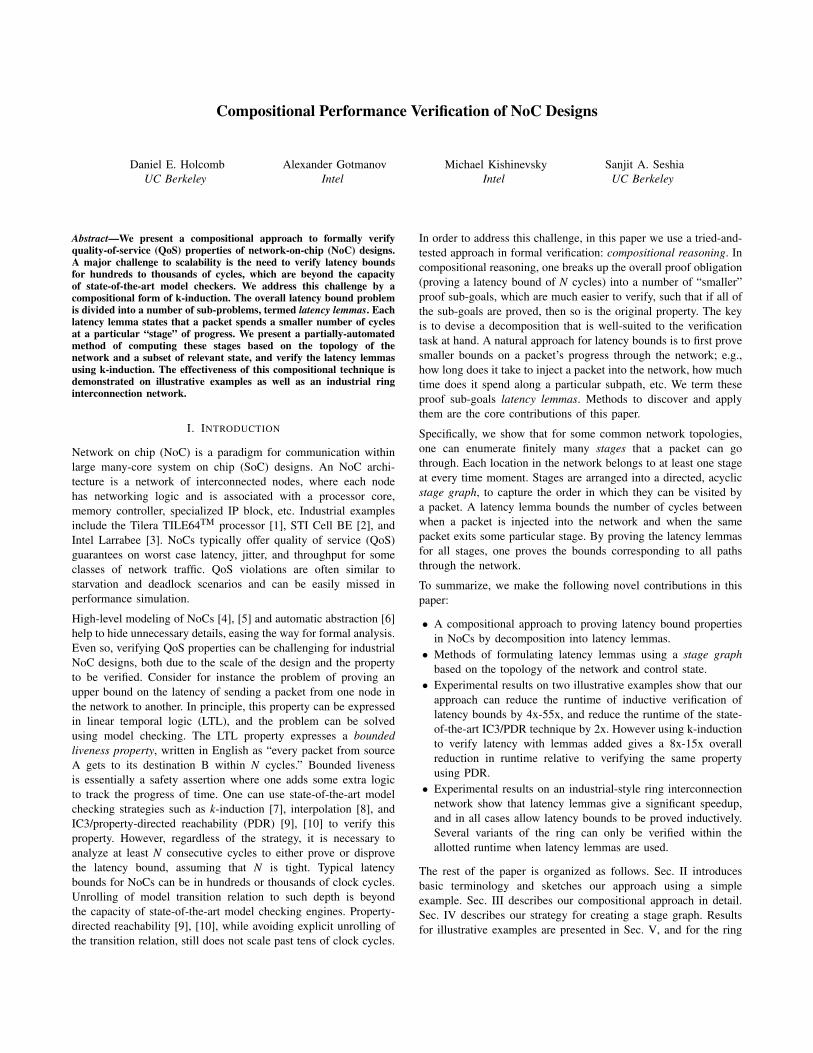
Figure 3: Correspondence between network N and stage graph G.

also hold in the next cycle. The conjunction of all latency lemmascomprises an inductive invariant for the age of all packets. As aninductive invariant, the property can be verified efficiently withouta high degree of unrolling. While this toy example might beverified using (one-step) induction, in general we construct sets ofcomposable lemmas that are verifiable with k-induction. The valuesof k are small on account of the latency lemmas each describingonly a small increment of progress. Useful latency lemmas canbe automatically discovered in many acyclic networks, and can bediscovered with the help of manual insight in cyclic networks.

III. FORMALISM

As sketched in the previous section, we use a set of conjecturedlatency lemmas in order to efficiently verify a bound on the end-to-end latency from any source in the network to any sink.

The model being verified is xMAS model N . We assign a uniqueindex i to every queue slot in the network, and let variable qi refer tothe content of the ith queue slot. The complete state of a networkN with L total queue slots comprises variables q0,q1, . . . ,qL−1representing slot contents, and some additional control variables.

A. Mapping from N to G

Let graph G = (S,E) be an acyclic digraph, with its verticess0,s1, . . . ,sM ∈ S called stages. Each stage corresponds to a latencylemma. Queue slots in N map to stages in G depending on state;all sinks in N map to special stage s0. If a slot i maps to stage j,then it means that slot i is subject to the jth latency lemma. Thereexists an edge e j,k ∈ E if a packet can occupy slots in N that mapto stages s j and sk in consecutive cycles.

In each state of execution, every queue slot in N that stores apacket is mapped to some stage in G (Fig. 3). A single queueslot can map to different stages depending on the state of certainvariables, but always maps to exactly one stage unless the slot isempty. The mapping is defined using a set of formulas pi, j. Eachformula refers to a particular slot i in N and stage s j ∈G, and istrue if the packet in slot i maps to stage s j. In other words, pi, j isthe Boolean function defining conditions under which slot i mapsto stage j, and the function takes as inputs variables qi ∈ Qi andc ∈C.

Latency lemmas for a given slot are forbidden from consideringthe contents of any other slots so as to avoid the correspondingblow-up in the number of stages of G. This restriction on the formof latency lemmas can introduce looseness in the latency boundsby forcing each packet to always make conservative assumptionsabout other traffic.

pi, j : Qi×C 7→ B (1)

• Qi is the set of states of queue slot i.• C is the set of states of the control variables used to enforce fair-

ness, including priority bits of merge primitives and reservationstates of control logic.

A few special cases are worth mentioning. If slot i can never mapto stage s j then pi, j = false regardless of qi and c. If slot i alwaysmaps to stage s j, then pi, j = true, regardless of qi and c. We saysome combination of slot i and states (qi,c) are covered by stages j if formula pi, j = true for (qi,c). Alternatively, we sometimessay that a packet is covered by s j if it resides in the slot i at a timewhen pi, j is true.

All packets in all reachable states should be covered by some stagein G during every cycle. For each slot i, assume the existence of aspecification variable usedi that is true in every state where slot istores a packet. A coverage property X is defined as true if everyused slot i in N maps to at least one stage in G.

X :=∧

i∈[0,L−1]

usedi =⇒

∨s j∈S

pi, j

B. Latency Lemmas to Imply Global Latency Bound

The xMAS model N is augmented with a global clock and packettimestamps to allow latency bounds to be evaluated as safetyproperties over single states. The current time clk and the injectiontimestamps t(qi) are specification variables in the xMAS model.Variable clk is the state of an n-bit counter that increments duringevery cycle. The timestamp is created by appending the currentvalue of clk to every packet when it is first injected from a sourceinto the network. When a packet occupies slot i, its timestamp t(qi)is part of the slot’s state qi. Each queue slot in N is thereforewidened by n-bits to accommodate the packet timestamps.

The global latency bound property and the latency lemmas bothassert claims about the age of a packet. The age of the packet inslot i (denoted age(qi)), is the difference between the current timeand the packet’s timestamp (Eq. 2). Property ΦG (Eq. 3) asserts thatno packet has an age of TV ER. Latency lemma φ j (Eq. 4) assertsthat any packet in a slot i that satisfies pi, j (i.e. maps to stage s j)has an age less than Tj. Property ΦL (Eq 5) asserts that all latencylemmas hold.

age(qi) := (clk− t(qi)) mod 2n (2)

ΦG :=

∧i∈[0,L−1]

(usedi =⇒ age(qi) < TV ER) (3)

φ j :=∧

i

(pi, j =⇒ age(qi) < Tj

)(4)

ΦL :=

∧j

φ j (5)

Latency lemmas are helpful because their composable nature allowsthem to be verified without a large number of unrollings. Whilethe packet timestamps are ostensibly added to a packet when it isinjected, the general initial state of induction allows for packets toexist without being injected3. Because the latency lemmas constrainthe age of packets at intermediate stages of progress, it is notnecessary for the verifier to unroll the circuit to a depth that isproportional to the total path latency. Each lemma can essentiallyignore the prefix path, and assert an age bound building onlyupon the lemmas of direct predecessor stages. This simplificationprovides a large reduction in the number of unrollings requiredand in the solver runtime, but could introduce looseness into theverified bounds.

C. Automated Invariant Strengthening

An advantage of using the xMAS formalism is automated invariantstrengthening. The automatically generated invariants are unrelatedto QoS, but are useful to block the verifier from exploring unreach-able states. The set of inferred invariants is denoted Ψ, and can in-clude numeric invariants [5] and channel persistency invariants [11]among others. This work uses channel persistency invariants, non-blocking invariants on selected channels, and invariants to specifythat the head and tail pointer of each queue are consistent with thenumber of items stored in it.

Including the automated invariants and latency lemmas, the totalverification problem becomes N � ΦL ∧Ψ∧ΦG. The approachis sound because the verified property is a strengthening of theoriginal latency property ΦG.

IV. RULES FOR CONSTRUCTING STAGE GRAPH

The pi, j formulas that define latency lemmas can be chosento be more abstract or precise, and we do not offer a schemefor choosing an optimal level of abstraction. Two extreme casesmust be avoided in defining these formulas. A mapping that isunnecessarily precise may induce too large a stage graph G. Amapping that is too abstract can induce a cyclic graph, or a graphwhere single stages are too large to serve as effective sub-goals.Our approach is to define the mapping as abstractly as possibleusing simple mechanical rules, and to refine the mapping by case-splitting on fairness variables whenever graph G is cyclic or itssub-goals are too large.

A. Propagating Liveness Bounds in N

Latency depends largely on blocking caused by congestion. In anxMAS network, bounded liveness properties assert limits on theamount of blocking that can occur. Starting from the given livenessbounds of packet sinks in N , simple rules back-propagate theliveness bounds across primitives to obtain finite liveness boundsfor other channels.

For any persistent channel c, let dt(c) represent its liveness bound,or stated differently a bound on the number of consecutive cyclesin which the channel can be blocked. A claim of dt(c) = 2 isthen just a compact notation for temporal logic formula c.irdy =⇒

3These packets would have been injected prior to the current k framesof unrolling

F≤2c.trdy. For a non-blocking channel, dt(c) = 0. The livenessbounds dt(c) are not explicitly verified, but are instead only usedas a tool toward calculating the residence times of the stages in G.The rules to propagate liveness bounds through primitives to otherchannels are as follows:

1. Sink: For a sink with a liveness bound of x, dt(i) = x2. Queue: For a queue dt(i) = dt(o), indicating that the queue

itself does not add any backpressure beyond the backpressurefrom its output channel.4

3. Merge: In a fair merge primitive no input is ever blockedthrough a time period when the other merge input is grantedtwice, therefore dt(a) = dt(b) = 2dt(o)+1.

4. Switch: Without considering which output a packetwill be routed to, a conservative bound is given bydt(i) = max(dt(a),dt(b)).

B. Age Bounds of Stages in G

The liveness bounds of the previous subsection are a step towarddiscovering an age bound (Tj) for each latency lemma φ j. Let themaximum number of consecutive cycles during which a packet canmap to stage j be called the residence time of stage j, denoted byw j. If a queue slot i is the head of a queue primitive, and is the onlyslot that stage j can cover, then w j is one greater than the livenessbound on the output channel of the queue. Every stage coveringanother slot of this queue is assigned the same residence time,since non-head packets will advance within the queue wheneverthe head packet departs the queue (see Fig. 4). The age bound Tjfor a packet in any stage j is one greater than the sum of all theresidence times along the longest path to stage j (including j’s ownresidence time w j).

For topologically acyclic networks using the xMAS componentslisted above, the back-propagation scheme deduces liveness boundsfor all channels and maximum delays for each queue slot. The agebounds Tj can be obtained by dynamic programming in this acycliccase, as demonstrated in the tree saturation example of Subsec. V-C.

In cyclic networks, dynamic programming generates infinite Tjfor any stage j that is part of a cycle in G. The cycle can beeliminated by refining the stages using case-splitting on somefairness variables. A network that can guarantee finite latency mayalways have some refinement that produces an acyclic stage graph,but we make no claim about finding it automatically. In the ringexample of Sec. VI, we find that the fairness mechanisms used toensure finite latency are useful for verifying finite latency bounds.Automation of this refinement step is left to future work. Thering of Sec. VI is an example of a cyclic network that requiresrefinement. A similar refinement step can also be used to reducethe residence times of stages in acyclic networks, as is shown inthe tree saturation example (Subsec. V-C).

V. ILLUSTRATIVE EXAMPLES

Several illustrative examples are used to highlight strengths andweaknesses of the proposed approach. The first example is a

4A special case exists when a queue has size 1, disallows simultaneousread and write, and has an eager output channel. Under those conditions,dt(i) = 1 and dt(o) = 0.

single queue to introduce the approach, and the second showshow refinement can be used to reduce induction depth. In thesetwo examples, TV ER can be obtained mechanically with no manualinsight required. The ring network in Sec. VI will show an examplewhere insight is required.

A. Experiment Methodology

The methodology used across all experiments is described here.The xMAS models are written in word-level Verilog, with param-eterized modules implementing the xMAS primitives. The Verilogis bit-blasted into an and-inverter-graph5 (AIG) using the VeriABCflow [12]. Verification is performed on the AIG using the bit-levelmodel checker ABC [13]6 on a 2.4GHz Intel Core i5 processorwith 4GB of RAM. Both k-induction7 and property directedreachability8 (PDR) [10] are performed by ABC. The networksused in experiments are available online in both Verilog and AIGformat.9

Note that verification using k-induction consists of a base-case ofk frames of bounded model checking and an inductive step of kframes. When attempting to verify a property with k-induction,we do not know in advance what value of k will be necessary.We therefore take the conservative approach of allowing the basecase to explore a large number of frames kmax, and only learn kafter the verification terminates. Note that in all cases kmax ≥ k. Toavoid letting the arbitrary choice of kmax skew the runtimes, wereport only the runtime for the inductive step. The runtime of theinductive step is usually orders of magnitude larger than for thebase case.

The tightness of TV ER in each example is quantified using boundedmodel checking (BMC). Let TCEX be the largest latency for whichBMC can find a counterexample within some allotted resourcelimits. The smallest latency that can possibly be a valid latencybound is then TCEX + 1. Therefore, the maximum amount bywhich TV ER over-approximates the tightest possible latency boundis TV ER− (TCEX +1). The determination of TCEX for all examplesis given in Table IX in the appendix.

B. Single Queue

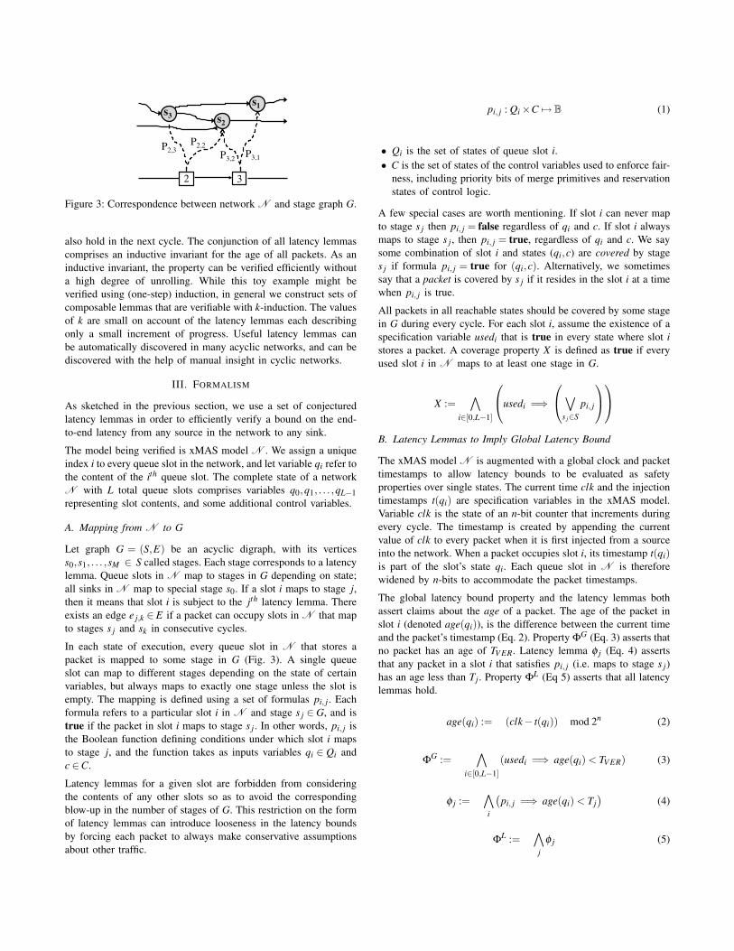
A queue of depth 5 is shown in Fig. 4, along with its stage graphG. The sink obeys a liveness bound of 2 cycles, while the source iscompletely non-deterministic. Each queue slot maps to one stage(Table I), and the age bound (Tj) for each stage is 3 cycles largerthan for the preceding stage.

The k-induction and PDR engines in ABC are both used toverify the latency (Tab. II). The first property is a conjunction ofthe latency lemmas (ΦL), the automatically generated invariants(Ψ), and the global latency bound (ΦG). K-induction verifies thisproperty 12X faster than does PDR. When latency lemmas areremoved from the property, the runtimes of both engines areincreased. Regardless of the engine used, strengthening the global

5http://fmv.jku.at/aiger6Rev. d0170182dbd6; at http://www.eecs.berkeley.edu/∼alanmi/abc/7ABC commands ”read aiger foo.aig; bmc3 -F kmax; orpos; ind -F kmax;”8ABC commands ”read aiger foo.aig; pdr -v;”9http://www.eecs.berkeley.edu/∼holcomb/memocode12 xmas.tar.gz

Queue$example$

s3!s5! s1!s2!13!10!

s4!7!

s0!

2!

16!4!

2! 1! 2! 3! 4! 5!

Figure 4: Queue with a sink obeying a livenessbound of 2 cycles, and corresponding stagegraph G.

j w j Tj pi, j(qi,c)1 3 16 p5,1 := true2 3 13 p4,2 := true3 3 10 p3,3 := true4 3 7 p2,4 := true5 3 4 p1,5 := true

Table I: Graph G from Fig 4. The index of eachstage is j. The residence time of each stage isw j. The age bound of each stage is Tj. Formulaspi, j define the mapping from N to G.

latency property using latency lemmas appears to create an easierverification problem.

Runtime (s) Frames Proved Engine Property1.24 5 Y kind ΦL ∧Ψ∧ΦG

4.50 17 Y kind Ψ∧ΦG

15.31 47 Y pdr ΦL ∧Ψ∧ΦG

41.96 45 Y pdr Ψ∧ΦG

129.00 53 Y pdr ΦG

Table II: Results for a queue of depth 5 and sink with livenessbound 2 (Fig. 4). In this example, TV ER = 16 and TCEX = 14(Tab. IX).

1) Varying Queue Depth: Next we repeat the verification ofproperty ΦL∧Ψ∧ΦG for different queue depths. In each case, thestage graph is modified according to the queue depth. The resultsare shown in Table III. Regardless of the queue depth, only 5 framesare required to verify the property using k-induction, because eachlatency lemma builds upon the lemmas for the other stages. Thenumber of frames required by PDR generally increases with thequeue depth.

K-ind PDRDepth Frames Run Time Frames Run Time

2 5 0.03 35 1.013 5 0.10 39 3.184 5 0.49 49 8.045 5 1.25 47 15.316 5 2.12 49 30.397 5 5.72 54 49.988 5 10.30 67 93.19

Table III: The runtime to verify N � ΦL ∧Ψ∧ΦG for differentqueue depths using k-induction and PDR.

2) Proving Lemmas in Isolation: A final experiment on a singlequeue is performed in order to investigate whether proving the

http://fmv.jku.at/aiger

http://www.eecs.berkeley.edu/~alanmi/abc/

http://www.eecs.berkeley.edu/~holcomb/memocode12_xmas.tar.gz

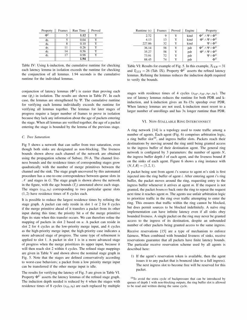
Property Frames Run Time ProvedΦL 5 1.12 Yφ5 5 0.04 Yφ4 8 0.10 Yφ3 11 0.26 Yφ2 14 0.56 Yφ1 17 0.98 Y

1.94

Table IV: Using k-induction, the cumulative runtime for checkingeach latency lemma in isolation exceeds the runtime for checkingthe conjunction of all lemmas. 1.94 seconds is the cumulativeruntime for the individual lemmas.

conjunction of latency lemmas (ΦL) is easier than proving eachone (φ j) in isolation. The results are shown in Table IV. In eachcase, the lemmas are strengthened by Ψ. The cumulative runtimefor verifying each lemma individually exceeds the runtime forverifying all lemmas together. The lemmas for later stages ofprogress require a larger number of frames to prove in isolationbecause they lack any information about the age of packets enteringthe stage. When all lemmas are verified together, the age of a packetentering the stage is bounded by the lemma of the previous stage.

C. Tree Saturation

Fig 5 shows a network that can suffer from tree saturation, eventhough both sinks are designated as non-blocking. The livenessbounds shown above each channel of the network are obtainedusing the propagation scheme of Subsec. IV-A. The channel live-ness bounds and the residence times of corresponding stages growquadratically with the number of merge primitives between thechannel and the sink. The stage graph uncovered by this automatedprocedure has a one-to-one correspondence between queue slots inN and stages in G. The stage graph is shown above the networkin the figure, with the age bounds (Tj) annotated above each stage.The stages (s10,s9) corresponding to two particular queue slots(1,2) have residence times of 8 cycles each.

It is possible to reduce the largest residence times by refining thestage graph. A packet can only reside in slot 1 or 2 for 8 cyclesif the merge primitive ahead of it transfers a packet from its otherinput during this time; the priority bit u of the merge primitiveflips its state when this transfer occurs. We can therefore refine themapping of packets in slot 2 based on u. A packet can reside inslot 2 for 4 cycles as the low-priority merge input, and 4 cyclesas the high-priority merge input; the high-priority case indicates amore advanced stage of progress. The same type of refinement isapplied to slot 1. A packet in slot 1 is in a more advanced stageof progress when the merge prioritizes its upper input, because itwill then reach slot 2 within 4 cycles. The refined stage mappingsare given in Table V and shown above the nominal stage graph inFig. 5. Note that the stages are defined conservatively accordingto worst-case behaviors; a packet from a low priority merge inputcan be transferred if the other merge input is idle.

The results for verifying the latency of Fig. 5 are given in Table VI.Property ΦL′ asserts the latency lemmas of the refined stage graph.The induction depth needed is reduced by 4 when the stages withresidence times of 8 cycles (s10,s9) are each replaced by multiple

Runtime (s) Frames Proved Engine Property

2.72 9 Y kind ΦL′ ∧Ψ∧ΦG

4.13 13 Y kind ΦL ∧Ψ∧ΦG

227.86 32 Y kind Ψ∧ΦG

36.14 58 Y pdr ΦL′ ∧Ψ∧ΦG

35.27 58 Y pdr ΦL ∧Ψ∧ΦG

73.91 72 Y pdr Ψ∧ΦG

88.45 74 Y pdr ΦG

Table VI: Results for example of Fig. 5. In this example, TV ER = 31and TCEX = 26 (Tab. IX). Property ΦL′ asserts the refined latencylemmas. Refining the lemmas reduces the induction depth requiredto verify the bounds.

stages with residence times of 4 cycles (s10′′ ,s10′ ,s9′′ ,s9′ ). Theuse of latency lemmas reduces the runtime for both PDR and k-induction, and k-induction gives an 8x-15x speedup over PDR.When latency lemmas are not used, k-induction must resort to alarger number of unrollings and has 3x longer runtime than PDR.

VI. NON-STALLABLE RING INTERCONNECT

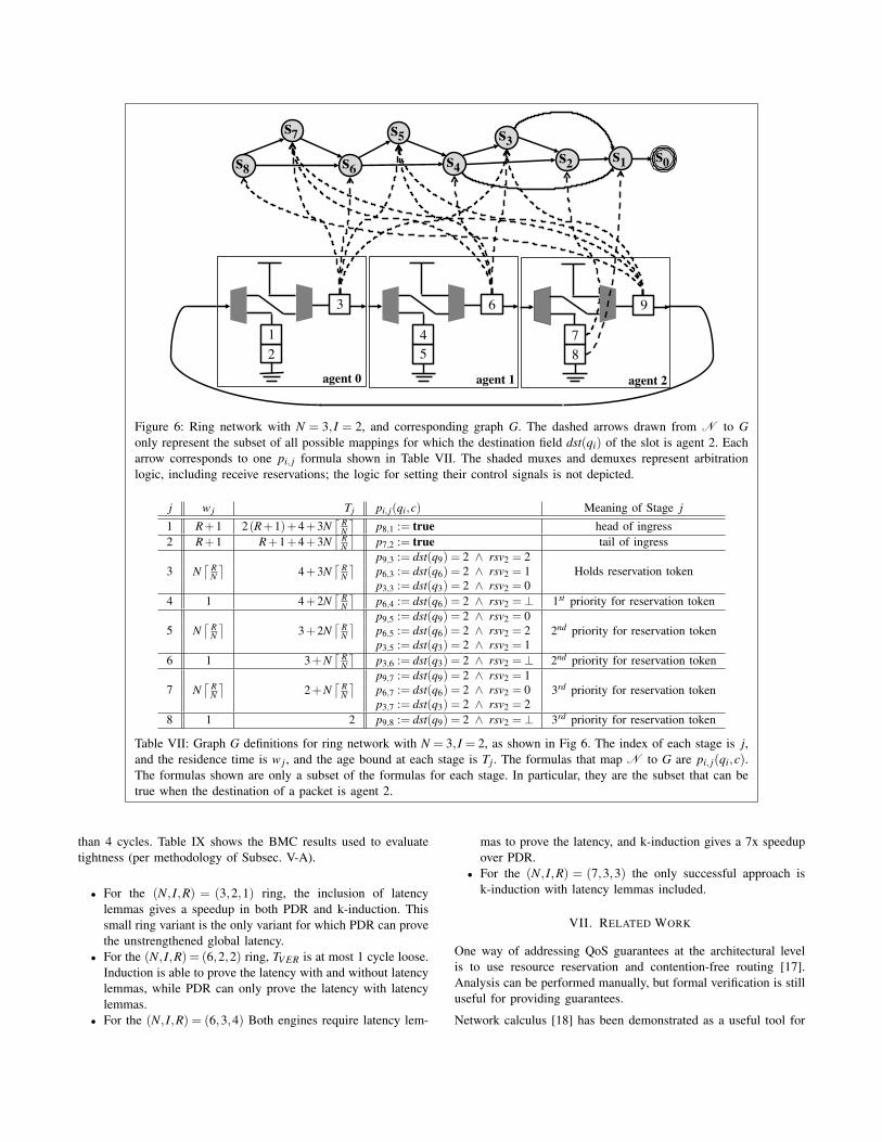
A ring network [14] is a topology used to route traffic among anumber of agents. Each agent (Fig. 6) comprises arbitration logic,a ring buffer slot10, and ingress buffer slots. Packets reach theirdestinations by moving around the ring until being granted accessto the ingress buffer of their destination agent. The general ringnetwork is configured by 3 parameters: the number of agents N,the ingress buffer depth I of each agent, and the liveness bound Ron the sinks of each agent. Figure 6 shows a ring instance with(N, I,R) = (3,2,1).

A packet being sent from agent i’s source to agent m’s sink is firstinjected into the ring buffer of agent i. After entering agent i’s ringbuffer, the packet moves around the ring, requesting entry to theingress buffer whenever it arrives at agent m. If the request is notgranted, the packet bounces back onto the ring to repeat the requestnext time it reaches agent m. The agents use unfair arbitration logicto prioritize traffic in the ring over traffic attempting to enter thering. This ensures that traffic within the ring cannot be blocked,but does permit sources to be blocked indefinitely. A naıve ringimplementation can have infinite latency even if all sinks obeybounded liveness. A single packet on the ring may never be grantedaccess to the ingress of its destination, despite an unboundednumber of other packets being granted access to the same ingress.

Receive reservations [15] are a type of mechanism to enforcefairness. When combined with bounded liveness of sinks, receivereservations guarantee that all packets have finite latency bounds.The particular receive reservation scheme used by all agents isdescribed here:

1) If the agent’s reservation token is available, then the agentissues it to any packet that is bounced (due to a full ingress).The next ingress slot to become free will be reserved for thispacket.

10To avoid the extra cycle of backpressure that can be introduced byqueues of depth 1 with non-blocking outputs, the ring buffer slot is allowedto be read and written during the same cycle.

s1!

1!

s4!

3!

s6!

s8!

u!

Ex_tree_sat!

s9!3!

s0!

s10!

1!

9!

s9’!s9”!s10’!s10”!13!

0!

s7!

s5!

s3!

s2!

0!0!1!1!

1!

3!

3!7!

7!

17! 21! 25!

27! 29!

5!

30! 31!

5! 9! 17!

1! 2! 3! 4! 5! 6!

7! 8!

9! 10!

7!

Figure 5: A network capable of tree saturation and the corresponding graph G. Channelannotations on N are liveness bounds, and stage annotations on G are the age bounds Tj.

j w j Tj pi, j(qi,c)1 1 31 p10,1 := true2 1 30 p9,2 := true3 2 5 p8,3 := true4 2 3 p7,4 := true5 2 29 p6,5 := true6 2 27 p5,6 := true7 4 25 p4,7 := true8 4 21 p3,8 := true9’ 4 17 p1,9′ := u9” 4 13 p1,9′′ := ¬u10’ 4 9 p1,10′ := u10” 4 5 p1,10′′ := ¬u

Table V: Details of refined graph Gfrom Fig 5. The index of each stageis j. The residence time of eachstage is w j. The age bound of eachstage is Tj. Formulas pi, j define themapping from N to G.

2) If the agent’s reservation token is outstanding, packets thatdo not hold it are denied access to the ingress buffer, unlessthe ingress buffer has more than 1 free slot.

3) When a packet with a receive reservation token is grantedaccess to the ingress buffer, the token is returned to the agent.

Receive reservations are fair with respect to packets in the ring.Whenever one packet returns the reservation token, the packettrailing it on the ring has a chance to make the reservation inthe subsequent cycle. Each packet in the ring gets a turn at makinga receive reservation in order.

The liveness bound of the sink is used as the basis for analyticalupper bound on the latency of the ring. Because each sink’s livenessbound of R back-propagates to the ingress’ input channel, noreceive reservation can be held by one packet for more than Nd R

N ecycles; if R < N for example, then any receive reservation that isissued will be returned exactly N cycles later when the reservingpacket returns. Given that there are N total slots in the ring, ananalytical upper bound on the age of any packet in the ring isgiven by tring in Eq. 6. An upper bound on the age of any packetin the entire network is given by TV ER in Eq. 7. It is important tonote that the analytical bound used for TV ER is derived from thehigh-level specification, but our approach allows it to be proved onthe bit-level (Verilog) implementation of the network.

tring = 1+N(

1+N⌈

RN

⌉)(6)

TV ER = I ∗ (R+1)+ tring (7)

Send reservation mechanisms [16] are a counterpart to receivereservations for ensuring fairness in granting ring slots to sources,but are not addressed in this work.

A. Generating a useful stage graph G

The existence of cyclic paths in N complicates the constructionof a stage graph, because the location of a packet within the

ring is not a sufficiently precise indicator of progress. To findsub-goals for marking progress of packets circling the ring, werefine the latency lemmas by case splitting on the state of receivereservations. The refinement based on receive reservation priorityin the ring is analogous to the refinement based on merge priorityin Subsec. V-C.

Some notation is required for the mapping from N to G in the ring.For each agent i∈ [0,N−1], let rsvi ∈ {⊥,0,1, . . . ,N−1} indicatewhich of the N agents contains the ring slot holding the reservationtoken of agent i. rsvi =⊥ indicates that the receive reservation isavailable. For each queue slot j in N , let dst(q j) be the destinationaddress of the packet. The destination address is chosen for eachpacket non-deterministically at the time of injection, and is storedwith the packet in the same manner as the timestamp t(q j).

Using an (N, I,R) = (3,2,1) ring as an example, the definitionand explanation of the sub-goal for each stage in G is given inTable VII. We clarify notation by explaining the row of table VIIthat is denoted by j = 4; this row gives the age bounds and mappingconditions for stage 4. Only queue slot q6 can ever map to stage 4,and it does so only when formula p6,4 is true. Formula p6,4 is trueif the packet in slot q6 has agent 2 for its destination and agent 2has an available receive reservation. Stage 4 has a residence timeof 1 cycle. The packet mapping to stage 4 must have an age ofless than 4+2Nd R

N e.

B. Results

Our approach is evaluated on 4 different variants of the parame-terized ring. The timeout for each verification experiment is 10kseconds. The results are shown in Table VIII. Strengthening theglobal latency property (ΦG) by latency lemmas (ΦL) and auxiliaryinvariants (Ψ) allows the global latency bound of TV ER to be provedby k-induction in all cases within 700 seconds using 13 frames orless. The inclusion of latency lemmas also reduces the runtime ofPDR, but PDR is unable to verify 2 variants within the allottedtime even with latency lemmas included. The bounds proved in allcases do not over-approximate the tightest possible bound by more

ring_network!

ingress!

ring buffer!

agent 0!

s1!s2!

s3!

s4!

s5!

s6!s8!s0!

R!

s7!rsv!

Rsv avail!

agent 1! agent 2!

3!

4!8!7!

9!

2!1!

5!

6!

Figure 6: Ring network with N = 3, I = 2, and corresponding graph G. The dashed arrows drawn from N to Gonly represent the subset of all possible mappings for which the destination field dst(qi) of the slot is agent 2. Eacharrow corresponds to one pi, j formula shown in Table VII. The shaded muxes and demuxes represent arbitrationlogic, including receive reservations; the logic for setting their control signals is not depicted.

j w j Tj pi, j(qi,c) Meaning of Stage j

1 R+1 2(R+1)+4+3N⌈ R

N

⌉p8,1 := true head of ingress

2 R+1 R+1+4+3N⌈ R

N

⌉p7,2 := true tail of ingress

3 N⌈ R

N

⌉4+3N

⌈ RN

⌉ p9,3 := dst(q9) = 2 ∧ rsv2 = 2Holds reservation tokenp6,3 := dst(q6) = 2 ∧ rsv2 = 1

p3,3 := dst(q3) = 2 ∧ rsv2 = 04 1 4+2N

⌈ RN

⌉p6,4 := dst(q6) = 2 ∧ rsv2 =⊥ 1st priority for reservation token

5 N⌈ R

N

⌉3+2N

⌈ RN

⌉ p9,5 := dst(q9) = 2 ∧ rsv2 = 02nd priority for reservation tokenp6,5 := dst(q6) = 2 ∧ rsv2 = 2

p3,5 := dst(q3) = 2 ∧ rsv2 = 16 1 3+N

⌈ RN

⌉p3,6 := dst(q3) = 2 ∧ rsv2 =⊥ 2nd priority for reservation token

7 N⌈ R

N

⌉2+N

⌈ RN

⌉ p9,7 := dst(q9) = 2 ∧ rsv2 = 13rd priority for reservation tokenp6,7 := dst(q6) = 2 ∧ rsv2 = 0

p3,7 := dst(q3) = 2 ∧ rsv2 = 28 1 2 p9,8 := dst(q9) = 2 ∧ rsv2 =⊥ 3rd priority for reservation token

Table VII: Graph G definitions for ring network with N = 3, I = 2, as shown in Fig 6. The index of each stage is j,and the residence time is w j, and the age bound at each stage is Tj. The formulas that map N to G are pi, j(qi,c).The formulas shown are only a subset of the formulas for each stage. In particular, they are the subset that can betrue when the destination of a packet is agent 2.

than 4 cycles. Table IX shows the BMC results used to evaluatetightness (per methodology of Subsec. V-A).

• For the (N, I,R) = (3,2,1) ring, the inclusion of latencylemmas gives a speedup in both PDR and k-induction. Thissmall ring variant is the only variant for which PDR can provethe unstrengthened global latency.

• For the (N, I,R) = (6,2,2) ring, TV ER is at most 1 cycle loose.Induction is able to prove the latency with and without latencylemmas, while PDR can only prove the latency with latencylemmas.

• For the (N, I,R) = (6,3,4) Both engines require latency lem-

mas to prove the latency, and k-induction gives a 7x speedupover PDR.

• For the (N, I,R) = (7,3,3) the only successful approach isk-induction with latency lemmas included.

VII. RELATED WORK

One way of addressing QoS guarantees at the architectural levelis to use resource reservation and contention-free routing [17].Analysis can be performed manually, but formal verification is stilluseful for providing guarantees.

Network calculus [18] has been demonstrated as a useful tool for

(N, I,R) TCEX TV ER Runtime (s) Frames Proved Engine Property

(3,2,1) 12 17

4.89 7 Y kind ΦL∧Ψ∧ΦG

15.36 16 Y kind Ψ∧ΦG

56.84 84 Y pdr ΦL∧Ψ∧ΦG

99.20 82 Y pdr Ψ∧ΦG

119.89 77 Y pdr ΦG

(6,2,2) 47 49


377.73 51 Y kind Ψ∧ΦG

1874.63 152 Y pdr ΦL∧Ψ∧ΦG

10000.00 77 - pdr Ψ∧ΦG

10000.00 81 - pdr ΦG

(6,3,4)55 58


4838.04 61 Y kind Ψ∧ΦG

2555.98 149 Y pdr ΦL∧Ψ∧ΦG

10000.00 70 - pdr Ψ∧ΦG

10000.00 57 - pdr ΦG

(7,3,3)66 69


8573.73 71 Y kind Ψ∧ΦG

5960.78 165 Y pdr ΦL∧Ψ∧ΦG

10000.00 73 - pdr Ψ∧ΦG

10000.00 70 - pdr ΦG

Table VIII: Verifying global latency bound (ΦG) with and without latency lemmas (ΦL) and auxiliary invariants (Ψ)for four different variants of the parameterized ring. Values of TCEX are from Tab. IX. The timeout is 10k seconds.

NoC performance analysis [19]. However, it has limited applica-bility and precision for networks with backpressure and complexcircular message dependencies. Network calculus formalism relieson very high-level abstraction of arbiters, often modeling them aslatency-rate servers. Recent abstraction-based formal approacheshave been applied to NoC components [6], but they only addressscalability problems arising from size of the network, rather thanfrom proving a large latency bound, while the present workaddresses the latter issue.

Several works have explored (unbounded) liveness verificationof communication fabrics. The standard approach of verifyingliveness using a liveness-to-safety transformation [20] does notscale to large networks in practice [11]. Alternative approachesinclude reducing deadlock conditions to a set of equations [11],[21], and proving liveness using the help of intermediate safetyassertions [22].

Our verification approach is conceptually similar to ranking func-tions [23], i.e. numeric functions of model state that measureprogress toward some goal. Typically, ranking functions are usefulin proving termination or liveness properties, but they are alsoapplicable for latency bounds. In fact, our stage graph can beviewed as a structural description of a ranking function for themodel. Note, however, that stage graphs specify partial orders,rather than the linear orders that are typical for ranking functions.

VIII. CONCLUSION

This work presents a compositional approach to verifying latencybound properties of NoC designs. The key idea is to decomposethe overall proof into a finite number of latency lemmas, based onthe notion of stages that a packet can be in. The latency lemma

approach is applied to illustrative examples and an industrial ringdesign. The approach facilitates inductive verification of latencybounds, and also yields significant speedup when using the PDRalgorithm.

Acknowledgments. The authors thank Satrajit Chatterjee for tech-nical discussions, and Bob Brayton and his research group forassistance with tools. This research was supported in part by theGigascale Systems Research Center, one of six research centersfunded under the Focus Center Research Program (FCRP), aSemiconductor Research Corporation entity.

REFERENCES

[1] D. Wentzlaff, P. Griffin, H. Hoffmann, L. Bao, B. Edwards,C. Ramey, M. Mattina, C. Miao, J. Brown, and A. Agrawal,“On-chip interconnection architecture of the tile processor,” IEEEMicro, 2007.

[2] T. Chen, R. Raghavan, J. N. Dale, and E. Iwata, “Cell BroadbandEngine Architecture and its first implementation–A performanceview,” IBM Journal of Research and Development, vol. 51, no. 5,pp. 559–572, 2007.

[3] L. Seiler, D. Carmean, E. Sprangle, T. Forsyth, P. Dubey, S. Junk-ins, A. Lake, R. Cavin, R. Espasa, E. Grochowski, T. Juan,M. Abrash, J. Sugerman, and P. Hanrahan, “Larrabee: A Many-Core x86 Architecture for Visual Computing,” IEEE Micro,vol. 29, no. 1, pp. 10–21, 2009.

[4] S. Chatterjee, M. Kishinevsky, and U. Y. Ogras, “Quick FormalModeling of Communication Fabrics to Enable Verification,” inHigh Level Design Validation and Test Workshop, 2010.

[5] S. Chatterjee and M. Kishinevsky, “Automatic Generation ofInductive Invariants from High-Level Microarchitectural Modelsof Communication Fabrics,” in Computer Aided Verification,2010.

[6] D. E. Holcomb, B. A. Brady, and S. A. Seshia, “Abstraction-Based Performance Analysis of NoCs,” Design Automation Con-ference, Jun. 2011.

[7] M. Sheeran, S. Singh, and G. Stalmarck, “Checking safetyproperties using induction and a SAT-solver,” in Formal Methodsin Computer-Aided Design, 2000, pp. 108–125.

[8] K. L. McMillan, “Interpolation and SAT-based model checking,”in Computer Aided Verification, 2003, pp. 1–13.

[9] A. R. Bradley, “SAT-Based Model Checking Without Unrolling,”Verification, Model Checking, and Abstract Interpretation, 2011.

[10] N. Een and A. Mishchenko, “Efficient implementation of propertydirected reachability,” in Proceedings of International Workshopon Logic Synthesis, 2011.

[11] A. Gotmanov, S. Chatterjee, and M. Kishinevsky, “Verify-ing Deadlock-Freedom of Communication Fabrics,” Verification,Model Checking, and Abstract Interpretation, 2011.

[12] J. Long, S. Ray, B. Sterin, and A. Mishchenko, “EnhancingABC for LTL Stabilization Verification of SystemVerilog/VHDLModels,” International Workshop on Design and Implementationof Formal Tools and Systems, 2011.

[13] R. Brayton and A. Mishchenko, “ABC: An Academic Industrial-Strength Verification Tool,” Computer Aided Verification, 2010.

[14] W. J. Dally and B. Towles, Principles and Practices of Intercon-nection Networks.

[15] M. Mattina, G. Chrysos, and S. Felix, “Method and apparatusfor synchronous unbuffered flow control of packets on a ringinterconnect,” US Patent 7,539,141, May 2009.

[16] M. Mattina, G. Chrysos, and Y. Choi, “Method and apparatusfor preventing starvation in a slotted-ring network,” US Patent7,733,898, Jun. 2010.

[17] K. Goossens, J. Dielissen, and A. Radulescu, “Æthereal networkon chip: concepts, architectures, and implementations,” IEEEDesign & Test of Computers, vol. 22, no. 5, pp. 414–421, Sep.2005.

[18] R. L. Cruz, “A calculus for network delay, part I. Networkelements in isolation,” IEEE Transactions on Information theory,vol. 37, no. 1, pp. 114–131, 1991.

[19] M. H. Wiggers, M. J. G. Bekooij, and G. J. M. Smit, “Modellingrun-time arbitration by latency-rate servers in dataflow graphs,” in10th Workshop on Software & Compilers for Embedded Systems.New York, NY, USA, 2007, pp. 11–22.

[20] A. Biere and C. Artho, “Liveness Checking as Safety Checking,”Electronic Notes in Theoretical Computer Science, 2002.

[21] F. Verbeek and J. Schmaltz, “Hunting deadlocks efficiently inmicroarchitectural models of communication fabrics,” FormalMethods in Computer-Aided Design, 2011.

[22] S. Ray and R. K. Brayton, “Scalable Progress Verification inCredit-Based Flow-Control Systems,” Design Automation andTest in Europe, 2012.

[23] A. Turing, “Checking a large routine,” Conference on High SpeedAutomatic Calculating Machines, 1949.

APPENDIX: BOUNDED MODEL CHECKING

The results of Table IX show the set of experiments conducted toobtain TCEX for each network N . For each N , TCEX is set tobe the largest T (shown in bold) for which a counterexample isdiscovered by bounded model checking. All properties except forΦG are omitted in BMC. A linear search of T over the range[0,TV ER] is performed; the linear search is chosen over binarysearch to minimize the number of trials that have a potentiallyexpensive time-out. For each T that is tested, the BMC run endswhen one of the following conditions occurs:

1) A counterexample is found to show that T is an invalidbound. The number of frames explored to find the coun-terexample is shown.

2) 100 Frames of BMC are completed in less than 10k secondswithout finding a counterexample.

3) 10k Seconds have elapsed without finding a counterexampleand without completing 100 frames of BMC. As 100 framesare not yet reached, the number of frames explored withinthe 10k seconds is shown.

ex queue.v

T Found CEX Runtime(s) Frames12 Y 0.76 1813 Y 0.96 1914 Y 1.66 2115 - 2285.31 100

ex tree sat.v


ring 321.v


ring 622.v


ring 634.v


ring 733.v


Table IX: Search with bounded model checking to discover TCEXfor each N

compositional performance veriﬁcation of noc designs

Documents