Compositional Recurrence Analysis Revisited ∗

Zachary KincaidPrinceton Univ.

zkincaid@cs.princeton.edu

Jason Breck Ashkan ForouhiBoroujeni

Univ. of Wisconsin{jbreck,ashkanfb}@cs.wisc.edu

Thomas RepsUniv. of Wisconsin and GrammaTech,

Inc.reps@cs.wisc.edu

AbstractCompositional recurrence analysis (CRA) is a static-analysismethod based on an interesting combination of symbolic analy-sis and abstract interpretation. This paper addresses the problemof creating a context-sensitive interprocedural version of CRA thathandles recursive procedures. The problem is non-trivial becausethere is an “impedance mismatch” between CRA, which relies onanalysis techniques based on regular languages (i.e., Tarjan’s path-expression method), and the context-free-language underpinningsof context-sensitive analysis.

We address this issue by showing that we can make use of arecently developed framework—Newtonian Program Analysis viaTensor Product (NPA-TP)—that reconciles this impedance mis-match when the abstract domain supports a few special operations.Our approach introduces new problems that are not addressed byNPA-TP; however, we are able to resolve those problems. We callthe resulting algorithm Interprocedural CRA (ICRA).

Our experimental study of ICRA shows that it has broad overallstrength. The study showed that ICRA is both faster and handlesmore assertions than two state-of-the-art software model checkers.It also performs well when applied to the problem of establishingbounds on resource usage, such as memory used or execution time.

1. IntroductionStatic analysis provides a way to obtain information about thepossible states that a program reaches during execution, but withoutactually running the program on specific inputs. Two importantapproaches to static analysis are• abstract interpretation, in which the program is executed over

an abstract domain that (deliberately) leaves out certain detailsof concrete execution states so that the analyzer can explore a

∗ Supported, in part, by a gift from Rajiv and Ritu Batra; by AFRL un-der DARPA MUSE award FA8750-14-2-0270 and DARPA STAC awardFA8750-15-C-0082; and by the UW-Madison Office of the Vice Chancel-lor for Research and Graduate Education with funding from the WisconsinAlumni Research Foundation. Any opinions, findings, and conclusions orrecommendations expressed in this publication are those of the authors, anddo not necessarily reflect the views of the sponsoring agencies. T. Reps hasan ownership interest in GrammaTech, Inc., which has licensed elements ofthe technology reported in this publication.

[Copyright notice will appear here once ’preprint’ option is removed.]

program’s behavior for all possible inputs and all states that theprogram can reach (as well as some unreachable states);• symbolic analysis, which uses logical formulas to create precise

models of a program’s actions, but is usually forced to forgo anexploration that accounts for all of the reachable states.Compositional recurrence analysis (CRA) [13] is a static-

analysis method based on an interesting combination of symbolicanalysis and abstract interpretation. It performs abstract interpreta-tion using an abstract domain of transition formulas, and thus workswith quite precise models of a procedure’s actions. It carries out abottom-up exploration that accounts for all of a procedure’s reach-able states by performing a non-trivial abstraction step at each loop:the formula for the loop body is converted into a system of linearrecurrences, which are then solved to create a summary transformerthat involves polynomial constraints. So that the analyzer can con-tinue its bottom-up analysis—proceeding upward to analyze theloop’s context—the summary transformer is converted into a tran-sition formula.

The CRA domain meets the conditions required to apply Tar-jan’s path-expression method [33] for solving single-proceduredataflow-analysis problems. For each node n, a regular expressionRn is created that summarizes all paths from entry to n. In CRA,the regular expressions are then evaluated using an interpretation ofthe regular operators +, ·, and ∗ as disjunction, sequential compo-sition, and the generation and solving of an appropriate system ofrecurrence equations, respectively.

CRA is compositional in the sense that it computes the abstractmeaning of a program by computing, and then combining, theabstract meanings of its parts.• At the intraprocedural level, CRA makes use of Tarjan’s path-

expression method to compose the meanings of sub-parts via theinterpretations of +, ·, and ∗ [13].• At the interprocedural level, each procedure is analyzed indepen-

dently of its calling context to produce a summary that is used tointerpret calls to the procedure.

However, CRA is non-uniform: although recursion is a kind of gen-eralized loop construct, the algorithm that CRA uses to summarizeloops (based on generating and solving recurrences) is not the sameas the one it uses to summarize recursive procedures (which relieson coarse abstraction and widening). For instance, if a loop is re-coded using a tail-recursive procedure, CRA is not able to identifythe same numeric invariants in the recursive version that it identifiesin the version with an explicit loop.

This paper addresses the problem of creating a context-sensitiveinterprocedural version of CRA that handles loops and recursion—including non-linear recursion—in a uniform way. To solve thisproblem, we must deal with the “impedance mismatch” betweenCRA’s reliance on Tarjan’s path-expression method, which handlesregular languages, and the context-free-language underpinningsof context-sensitive interprocedural analysis [5, 14, 27, 28, 31].This issue is challenging because at the technical level, the regular-

1 2016/10/6

language viewpoint is baked into CRA: CRA’s recurrence-solvingstep is coupled with the interpretation of Kleene-star ( ∗).

The inspiration for our work was to use the recently devel-oped framework for Newtonian Program Analysis via Tensor Prod-uct (NPA-TP) [29] to address the aforementioned impedance mis-match. At first blush, it appeared that NPA-TP overcomes theimpedance mismatch because it provides a way to harness Tarjan’spath-expression method for interprocedural analysis: NPA-TP hasthe surprising property of converting an interprocedural-analysisproblem—i.e., a context-free path problem—into a sequence ofregular-language path problems.

For NPA-TP to be applicable, the abstract domain must sup-port a few non-standard operations (i.e., a so-called tensor-productoperation and a detensor operation). While the CRA domain doessupport these non-standard operations (see §4.3), it fails to meetsome “standard” properties. CRA unfortunately has infinite ascend-ing chains, and thus NPA-TP[CRA] would not be guaranteed to ter-minate. Moreover, CRA does not have an effective entailment pro-cedure, and thus it is not possible, in general, to ascertain whetheran NPA-TP[CRA] analyzer has reached a fixed point.

We address these issues by developing an algorithm that adopts,but adapts in significant ways, ideas used in the NPA-TP frame-work. (See §4.4.) The resulting algorithm, which we call NPA-TP-GJ (Alg. 4.17) extends the ideas of NPA-TP to make it even moregenerally applicable: Kleene iteration, NPA, and NPA-TP do notconverge at all for the class of domains considered by NPA-TP-GJ(and in particular, the CRA domain). The problem that NPA-TP-GJ addresses is how to both detect and enforce convergence whenworking with an abstract domain that has neither decidable equiva-lence nor the ascending-chain condition.

NPA-TP-GJ has broad overall strength. Our experimentsshowed that NPA-TP-GJ instantiated for Interprocedural CRA(ICRA) is both faster and handles more assertions than two state-of-the-art software model checkers. (See §5.1.)

ICRA also provides a new, systematic approach to the problemof establishing bounds on resource usage, such as memory used orexecution time. Recent work by Hoffmann et al. [6, 20] on estab-lishing resource-usage bounds is able to provide polynomial upperbounds on the resource usage of programs with several arguments.It can even succeed when the bound requires an amortized-costanalysis. Hoffmann et al. use ad hoc techniques to analyze pro-cedures (and recursive procedures), whereas ICRA is based on theclassical idea of creating behavior summaries for procedures, in-cluding recursive procedures. In the case of resource-bound anal-ysis, the summary for a procedure P characterizes the change inavailable resources caused by invoking P (and all procedures tran-sitively invoked by P ). Moreover, by approaching resource-boundanalysis as a problem of finding invariant polynomial inequalities,ICRA is able to obtain lower bounds on the resources used, as wellas upper bounds, in a uniform way. (See §5.2.)

Contributions. Overall, our work makes three main contribu-tions:• We extend CRA to create a context-sensitive interprocedural

version that handles loops and recursion—including non-linearrecursion—in a uniform way (§4.3 and §4.4).• We define an alternative to NPA-TP that can be used when the ab-

stract domain of interest has infinite ascending chains and doesnot support effective entailment (§4.4). The method retains sev-eral ideas from NPA-TP, including that of using tensor productsto rearrange the terms appearing in a system of (in)equations sothat certain operations can be postponed.• We report on the results of an experimental study (§5). The study

showed that ICRA is both faster and handles more assertions thantwo state-of-the-art software model checkers. ICRA also per-

forms well when applied to the problem of establishing resource-usage bounds.

Related work is discussed in §6. §7 concludes.

2. Background2.1 Compositional Recurrence Analysis (CRA)Tarjan’s path-expression method [33] is an alternative to the clas-sic iterative style of program analysis. In the iterative style, a pro-gram analysis is described by a lattice of program properties andan abstract transformer over the lattice. An abstract meaning of aprogram is computed by iterating the abstract transformer until afixed point is reached (possibly using a widening operator to en-sure convergence) [9]. In the algebraic style (following Tarjan), aprogram analysis is described by a semantic algebra: an algebraicstructure whose elements represent path properties, and which isequipped with operators for composing properties via sequencing(⊗), choice (⊕), and Kleene-star ( ∗). Computing an abstract mean-ing of a program can be seen as a two-step process. The first stepcomputes a path expression for the program, which is a regularexpression that recognizes the set of paths through the program’scontrol-flow graph. The second step evaluates the path expressionover the semantic algebra (i.e., using the algebra’s operations to in-terpret the regular-expression operations) to arrive at a property thatholds for all paths recognized by the path expression.

CRA follows this algebraic style [13]. The space of programproperties supported by CRA (i.e., the carrier of the semantic alge-bra of CRA) is the set of transition formulas over (not necessarilylinear) integer arithmetic. Letting x denote a finite set of programvariables, a transition formula φ(x,x′) is a formula over the vari-ables x plus a set of primed copies x′, representing the values ofthe variables before and after executing a path. The sequencing op-eration is relational composition and choice is disjunction.1

φ⊗ψ def= ∃x′′.φ(x,x′′) ∧ ψ(x′′,x′) φ⊕ψ def

= φ ∨ ψ

The heart of CRA is its iteration operator. Given as input atransition formula φbody that summarizes the body of a loop, theiteration operator computes a formula φ∗body that summarizes anynumber of iterations. The iteration operator works by using an SMTsolver to extract a system of recurrences entailed by φbody, and thenusing the closed form of the system as the abstraction of the loop.

We illustrate the high-level idea of how CRA analyzes loopsusing the example below. (See [13] for algorithmic details.)

while (i > 0)i := i - 1if (*) x := x + ielse y := y - i

CRA computes a transition formula for the above loop by applyingthe iteration operator to a transition formula representing its body:

φbody : i > 0 ∧ i′ = i− 1 ∧

((x′ = x + i ∧ y

′ = y)

∨ (x′ = x ∧ y′ = y− i)

).

The iteration operator extracts the following recurrence(in)equations from φbody, and computes their closed formsusing symbolic summation:

1 In the implementation of sequential composition (and that of the detensor-transpose operation defined in §4.3), fresh Skolem constants are introducedfor existentially quantified variables. We do not perform quantifier elimina-tion because the formulas are in non-linear integer arithmetic, which doesnot admit quantifier elimination.

2 2016/10/6

Recurrence Closed formi′ = i− 1 i(k) = i(0) − kx′ ≥ x x(k) ≥ x(0)

y′ ≥ y− i y(k) ≥ y(0) − k(k + 1)/2− ki(0)x′ ≤ x + i x(k) ≤ x(0) + k(k + 1)/2 + ki(0)

y′ ≤ y y(k) ≤ y(0)

x′ − y′ = x− y + ix(k) − y(k) = x(0) − y(0)

+k(k + 1)/2 + ki(0)

(where i(k) denotes the value of i on the kth iteration of the loop).Finally, to compute a transition formula representing any number ofiterations of φbody, the iteration operator introduces an existentiallyquantified non-negative iteration variable k, and conjoins the closedform of every recurrence:

φ∗body : ∃k.k ≥ 0∧ i′ = i− k∧ x′ ≥ x∧ y′ ≥ y + k(k + 1)/2 + ki∧ x′ ≤ x + k(k + 1)/2 + ki∧ y′ ≤ y∧ x′ − y′ = x− y + k(k + 1)/2 + ki

CRA is compositional in the sense that it computes the abstractmeaning of a program by breaking it into parts, computing a mean-ing for each part, and then composing the meanings (via ⊗, ⊕, and∗). This property makes it a natural fit for interprocedural analysis,because a procedure can be analyzed independently of its context toproduce a summary that can be used to interpret its calls. Recursiveprocedures, however, present an obstacle. The set of paths througha program that uses recursion is not regular, but rather context-free[27, 31], which places recursive behavior beyond the scope of whatcan be analyzed using CRA’s iteration operator. Recently, however,Reps et al. [29] showed that when a semantic algebra also providesa tensor-product operation, tensor-products can be used to convertlinear context-free systems of (in)equations into regular systems of(in)equations, opening the door to applying CRA’s loop analysis torecursive procedures.

2.2 Newtonian Program Analysis via Tensor Product(NPA-TP)

Esparza et al. [11, 12] generalized Newton’s method—the classi-cal numerical-analysis algorithm for finding roots of real-valuedfunctions—to a method, called Newtonian Program Analysis(NPA), for finding fixed-points of systems of inequalities oversemirings. NPA provides a new way to solve interproceduraldataflow-analysis problems. As in its real-valued counterpart, eachiteration of NPA solves a simpler “linearized” problem.

NPA solves systems of polynomial inequalities over semirings.Program-analysis problems give rise to such systems as follows:if P calls Q twice on some path, one has the inequality XP &XQ⊗XQ, which is quadratic. If there are actions a, b, and c beforeand after the calls, the inequality would be

XP & a⊗XQ⊗ b⊗XQ⊗ c. (1)

In contrast, an inequality is linear2 if each summand on the right-hand side contains only a single occurrence of a variable. For

2 In this paper, there is the potential for confusion between similar termsthat are used for different things in CRA and NPA-TP. In particular, in thecontext of NPA-TP, “linear” and “polynomial” refer to the number of oc-currences of variables on the right-hand sides of inequalities that capturea language of paths through the program. In the context of CRA, “linear”and “polynomial” refer to the properties of terms in the arithmetic transi-tion formulas that encode individual statement actions, loop summaries, orprocedure summaries. The intended meaning should be clear from context.

instance, the following (recursive) linear inequality

XP &(a⊗XQ⊗ b)⊕(c⊗XQ⊗ d)

⊕ (e⊗XR⊗ f)⊕(g⊗XP ⊗h).

corresponds to P calling Q twice in different branches, R once ina third branch, and P once in yet a fourth branch.

NPA is “Newtonian” because—like Newton’s method for nu-merical analysis—it performs a succession of rounds; on eachround, it uses a linear model (a “differential”3)—built from the sys-tem of inequalities, together with the current approximation to theanswer—to find the next approximation to the answer.

Operationally, NPA performs a kind of “linear-language sam-pling” of the state space of a program: if procedure P has multiplecall-sites along a given path, then the linearized program used dur-ing a given round of Newton’s method allows the analyzer to sam-ple the state space of P by taking the ⊕ of various linear-languagepaths through P . Along each such path through P , the abstract val-ues for the call-sites encountered are held fixed, except for possiblyone call-site on the path, which is explored by visiting (the linearmodel of) the called procedure. The abstract value for P and allother procedures are updated according to the results of this state-space exploration, and the algorithm proceeds to the next Newtonround. For instance, for Eqn. (1), the linear model would be

YP & (a⊗ νQ⊗ b⊗YQ⊗ c)⊕(a⊗YQ⊗ b⊗ νQ⊗ c)(where νQ denotes the value for YQ obtained on the previousround), which has just the one variable YQ in each summand.

A program with recursion is modeled with a recursive inequal-ity, e.g.,

X & d⊕ a⊗X ⊗ b⊗X ⊗ c. (2)The associated linear model is the recursive linear inequality

Y & d⊕(a⊗ ν⊗ b⊗Y ⊗ c)⊕(a⊗Y ⊗ b⊗ ν⊗ c). (3)

There is an important difference between the dataflow-analysisand numerical-analysis contexts: when Newton’s method is usedon numerical-analysis problems, multiplicative commutativity isrelied on to rearrange expressions of the form “e⊗Y ⊗ f” into“e⊗ f ⊗Y .” An inequality of the form “Y & g⊕ e⊗ f ⊗Y ” issimilar to the right-linear grammar “Y → g | e f Y ,” whichcorresponds to the regular language L(Y ) = (ef)∗g. In contrast,when Newton’s method is used for interprocedural dataflow anal-ysis, the “multiplication” operation involves function composition,and hence is non-commutative: “Y & g⊕ e⊗Y ⊗ f” cannot berearranged into “Y & g⊕ e⊗ f ⊗Y .”

The inequality “Y & g⊕ e⊗Y ⊗ f” is similar to the linearcontext-free grammar “Y → g | e Y f .” The latter describes thelinear context-free language (LCFL) L(Y ) = {eigf i}, each wordof which has “mirrored symmetry.” Consequently, the linear mod-els that arise in NPA, such as Eqn. (3), correspond to LCFLs withmirrored symmetry (albeit somewhat more complicated mirroredsymmetry than L(Y )).

In a generalization of the work of Esparza et al. called Newto-nian Program Analysis via Tensor Product (NPA-TP), Reps et al.[29] presented a way to convert each LCFL problem into a regular-language problem. Their construction allows them to apply Tarjan’spath-expression method [33] as an interprocedural analysis engineon each Newton round.

Given that the language aibi is the canonical example of anLCFL that is not regular, the NPA-TP transformation sounds im-possible. The secret is that one is not working with words: the

3 In NPA, the notion of a “differential” is not based on freshman calculus(so no limits as ∆x → 0). Instead, NPA just adopts the rewriting rules forcreating differentials (which are similar to the familiar rules for differenti-ation) to define a transformation on expressions that is used to create thelinear model [11, 12, 29].

3 2016/10/6

Y Y

Y

f1

�

�� ��

f2

Z Z Z

(���⨀ f1)

(1t⨀�)

(��⨀ f2)

(a) (b)

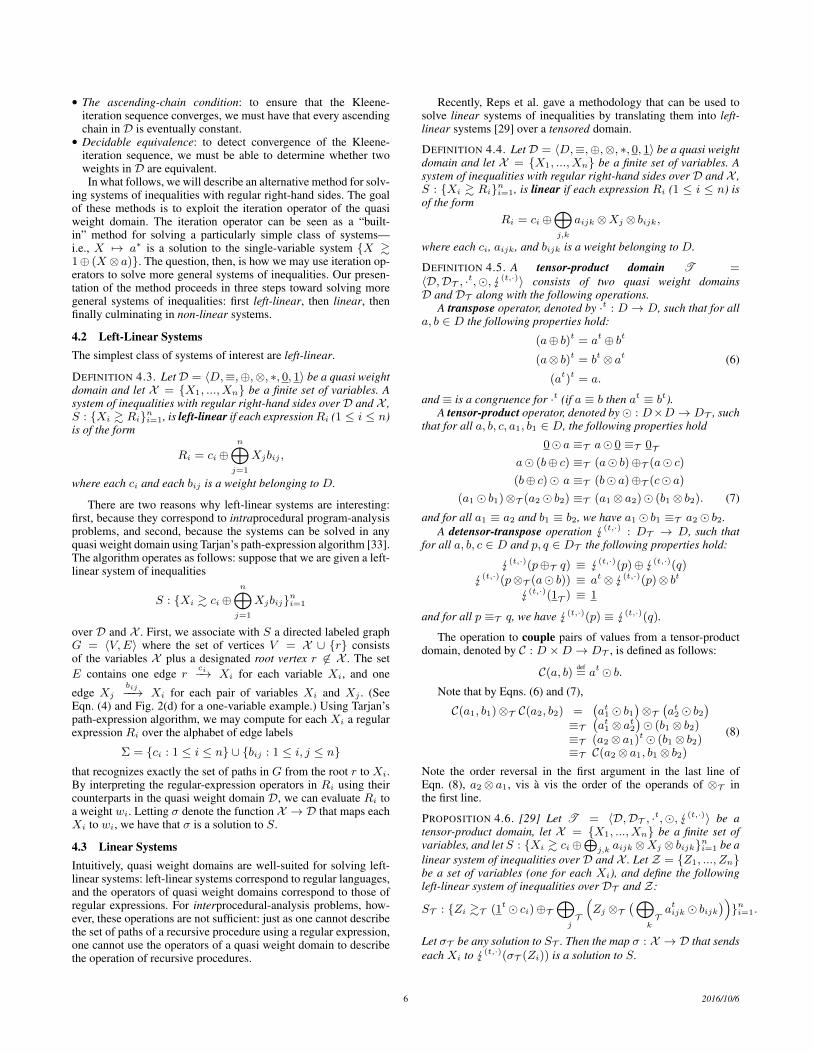
Figure 1: Graphical representations of (a) an unrolled LCFL path inthe Y system of inequalities; and (b) the corresponding unrolled regular-language path in the system of Z inequalities. The paths have the val-ues e2⊗ e1⊗ g⊗ f1⊗ f2 and (1t� g)⊗(et1� f1)⊗(et2� f2), respec-tively.

sum and product operations are interpreted. Also, NPA-TP requiresthe semiring to support a few additional operations—called “trans-pose” (·t), “tensor product” (�), and “detensor” ( (t,·))—that onedoes not have with words. However, one does have such opera-tions for predicate-abstraction problems (an important family ofdataflow-analysis problems used in essentially all modern-day soft-ware model checkers). In predicate-abstraction problems,• a semiring value is a square Boolean matrix• the product operation is Boolean matrix multiplication• the sum operation is pointwise “or”• transpose is matrix transpose, and• tensor product is Kronecker product.4

The key step in NPA-TP is to take each inequality of the form“Y & g⊕(e⊗Y ⊗ f)” in the linear model, and turn it into “Z &(1t� g)⊕(Z ⊗(et� f)),” using the operation λa.λb.(at� b) as akind of pairing operator. The reason why this transformation helpsis due to the following properties of ·t and �:

(a1⊗ a2)t = at2⊗ at1(a1� b1)⊗(a2� b2) = (a1⊗ a2)� (b1⊗ b2).

These properties cause each regular-language path in the Z systemto mimic an LCFL path in the Y system. For instance, theZ-systempath shown in Fig. 1(b) has the value

(1t� g)⊗(et1� f1)⊗(et2� f2) = (1t⊗ et1⊗ et2)� (g⊗ f1⊗ f2)= (e2⊗ e1⊗ 1)t� (g⊗ f1︸ ︷︷ ︸⊗ f2︸ ︷︷ ︸)

which has the kind of mirrored symmetry that we need to prop-erly track the symmetric correlations of values that arise in the Ysystem. More precisely, the detensor operation performs

(t,·)(et� f) = e⊗ f,

4 Each elementR of a predicate-abstraction domain can be thought of as anN ×N Boolean matrix

R =

r1,1 · · · r1,N...

. . ....

rN,1 · · · rN,N

.The Kronecker product of a square Boolean matrix is defined as follows:

R�S =

r1,1S · · · r1,NS...

. . ....

rN,1S · · · rN,NS

which is an N2 ×N2 binary matrix whose entries are

(R�S)[(a− 1)N + b, (a′ − 1)N + b′] = R(a, a′) ∧ S(b, b′).

void X() {if (?) sd;else {

sa;X();sb;X();sc;

}}

X

proc X

d b

c

X

a

proc Z

Z

(at?

bν

c)

Z

(1t?

d)

(at? bν c) ((aν b)t? c)

(1t?d)

�

(a) (b) (c) (d)

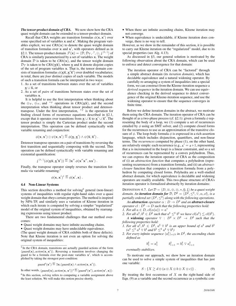
Figure 2: (a) Example program; (b) the program’s interproceduralcontrol-flow graph or, equivalently, the graphical representation of the cor-responding semiring inequality; (c) graphical representation of the lin-earized inequality for Z obtained using NPA-TP; (d) finite-state machinefor the valuations of all regular-language paths of the Z inequality, i.e.,(1t� d)((at� bνc)⊕((aνb)t� c))∗.

so that when the pair-value for the Z-system path is resolved intoa product, it has the mirrored symmetry of the LCFL path in the Ysystem shown in Fig. 1(a); i.e.,

(t,·)((e2⊗ e1⊗ 1)t� (g⊗ f1⊗ f2)) = e2⊗ e1⊗ 1⊗ g⊗ f1︸ ︷︷ ︸⊗ f2︸ ︷︷ ︸To use this idea to solve an LCFL path problem precisely, there

is one further requirement: the “detensor” operation must distributeover the (tensored) ⊕ operation. Because the Z system’s pathsencode all and only the LCFL paths of the Y system, the detensorof the ⊕-over-all-Z-paths equals the desired ⊕-over-all-Y -LCFL-paths. Reps et al. [29] showed that such a distributive detensoroperation exists for Kronecker products of Boolean matrices, andthus all the pieces fit together for predicate-abstraction problems.

EXAMPLE 2.1. To see how NPT-TP works end-to-end, considerthe program scheme shown in Fig. 2(a), which has a single recur-sive procedureX that uses four program statements: sa, sb, sc, andsd. Suppose that we have a semiring that captures a suitable ab-straction of the program’s actions (such as a predicate-abstractiondomain or the CRA abstract domain). Let a, b, c, and d denotethe semiring elements that abstract statements sa, sb, sc, and sd,respectively. The (abstract) actions of X can be expressed as therecursive inequality given as Eqn. (2). The graphical representa-tion of the inequality, shown in Fig. 2(b), can also be viewed as theprogram’s interprocedural control-flow graph (ICFG).

The linear model of Eqn. (2) that would be created with NPAis the recursive linear inequality given as Eqn. (3). In NPA-TP,Eqn. (3) is then converted into the following left-linear inequalityover tensored semiring elements:

Z &(1t� d)

⊕ Z ⊗((aνb)t� c)⊕ Z ⊗(at� bνc).

(4)

The graphical representation of Eqn. (4) is shown in Fig. 2(c).Because Eqn. (4) is left-linear, it corresponds to a regular lan-

guage of paths, and hence we can obtain a solution for Z in closedform. One way to obtain a solution is to create a finite-state ma-chine for the valuations of all regular-language paths of the Zinequality—see Fig. 2(d)—and then apply Tarjan’s path-expressionmethod [33] to obtain a regular expression for Z, namely,

Z = (1t� d)((at� bνc)⊕((aνb)t� c))∗.The above process is iterated by converting Z’s value into the

next approximant for ν (and hence for X) by ν = (t,·)(Z). In

4 2016/10/6

general, we want to find the least fixed-point of the inequality

ν & (t,·)((1t� d)((at� bνc)⊕((aνb)t� c))∗). (5)

The Newton-iteration sequence for X is thus the Kleene-iterationsequence for Eqn. (5).

ν(0) = 0

ν(1) = (t,·)((1t� d)((at� b0c)⊕((a0b)t� c))∗)= (t,·)((1t� d)(0)∗)

= (t,·)(1t� d)= d

ν(2) = (t,·)((1t� d)((at� bdc)⊕((adb)t� c))∗)...

3. Problem StatementThe problem addressed in the paper is the following:

Extend CRA to create a context-sensitive interprocedu-ral version (ICRA) that handles loops and recursion—including non-linear recursion—in a uniform way.

Our initial goal was to use NPA-TP because it provides a way toharness Tarjan’s path-expression method for interprocedural anal-ysis. This property meshes well with the way CRA couples itsrecurrence-solving step with the interpretation of Kleene-star.

Unfortunately, there is a mismatch between CRA and NPA-TP,which presented us with two substantial challenges:• The CRA domain has infinite ascending chains.• The problem of determining whether two CRA transition formu-

las are equivalent is undecidable.Consequently, if we merely instantiated the NPA-TP frameworkwith the CRA domain, the resulting algorithm would not be guar-anteed to converge, and even if it did converge, we would not nec-essarily know that it had.

The key insight that allowed us to devise an algorithm for ICRAis the following:

The iteration operator of CRA can be “factored” through asimple abstract domain (its iteration domain), which has de-cidable equivalence and a widening operator. We can trans-form a system of inequalities into special form such that theKleene-iteration sequence of the transformed system givesrise to a derived sequence in the iteration domain. We canthen use equivalence checking in the derived sequence todetect convergence of the iteration sequence of the revisedsystem, and use widening to ensure convergence in finitetime.

Our solution, presented in §4.4, retains the flavor of NPA-TP: inparticular, it adopts the idea of working with a simpler model of thesystem of inequalities, obtained by rearranging expressions usingtensor product (Prop. 4.12). However, other aspects are modifiedin significant ways. For instance, the key step of our method hasthe flavor Gauss-Jordan elimination: it repeatedly carries out (i)a symbolic variation of NPA-TP’s linearization step applied to asingle inequality, and (ii) substitution of a closed-form expressionfor the linearized symbol into the other inequalities (Alg. 4.13).

4. Technical Details4.1 Systems of InequalitiesThe following definition encapsulates the properties of CRA’s se-mantic algebra that we need to state the problem solved by the gen-eralization of NPA-TP presented in this paper.

DEFINITION 4.1. A quasi weight domain D = 〈D,≡,⊕,⊗, ∗, 0, 1〉 is a set D, equipped with an equivalence relation

≡, a binary combine operator ⊕, a binary extend operator ⊗, aunary closure operator ∗, and distinguished elements 0 and 1, thatsatisfies the following axioms.1. The equivalence relation ≡ is a congruence with respect to ⊕

and ⊗ (a1 ≡ a2 and b1 ≡ b2 implies a1⊕ b1 ≡ a2⊕ b2 anda1⊗ b1 ≡ a2⊗ b2). Note that≡ is not necessarily a congruencewith respect to the closure operator ∗.

2. 〈D,⊕,⊗, 0, 1〉 is an idempotent semiring “up to equivalence,”meaning that for all a, b, c ∈ D we have(a) (Associativity) (a⊗ b)⊗ c ≡ a⊗(b⊗ c) and (a⊕ b)⊕ c ≡

a⊕ (b⊕ c)(b) (Unit) a⊗ 1 ≡ 1⊗ a ≡ a and a⊕ 0 ≡ 0⊕ a ≡ a(c) (Commutativity) a⊕ b ≡ b⊕ a(d) (Distributivity) a⊗(b⊕ c) ≡ (a⊗ b)⊕ (a⊗ c) and

(b⊕ c)⊗ a ≡ (b⊗ a)⊕ (c⊗ a)(e) (Idempotence) a⊕ a ≡ a

3. The closure operator over-approximates reflexive transitive clo-sure, in the following sense. The combine operator of D definesa natural preorder . on D, where for any a and b in D, a . bif and only if a⊕ b ≡ b.(a) (Reflexivity) 1 . a∗

(b) (Transitivity) a∗⊗ a . a∗ and a⊗ a∗ . a∗

Because ⊗ will be used to model sequencing of program ac-tions, there is no assumption that ⊗ is commutative. To simplifynotation, we sometimes abbreviate a⊗ b as ab, and we assume thefollowing precedences for operators: ∗ > ⊗ > ⊕. We also some-times use a ∈ D rather than a ∈ D.

Note that we expect the⊕,⊗, and ∗ operators of a quasi weightdomain to be effective, but the equivalence relation need not be.The equivalence relation is used for developing the underlyingtheory of NPA-TP, but does not play a role in any algorithms.

The central question of interest in this paper is how to computesolutions, over quasi weight domains, to systems of inequalitieswith regular right-hand sides? The problem is formalized below.

DEFINITION 4.2. LetD = 〈D,≡,⊕,⊗, ∗, 0, 1〉 be a quasi weightdomain and let X = {X1, ..., Xn} be a finite set of variables. Asystem of inequalities with regular right-hand sides over D andX consists of one inequality for each variable

X1 & R1 · · · Xn & Rn

where each Ri is a regular expression over D and X . (That is, Ri

is a regular expression over an alphabet where each letter is eithera variable Xi or a weight w ∈ D.) More compactly, we write

S : {Xi & Ri}ni=1

to denote that S is the above system of inequalities with regularright-hand sides.

A solution to S is any map σ : X → D such that for eachXi ∈ X , we have σ(Xi) & σ(Ri), where σ(Ri) denotes thenatural extension of σ to regular expressions over D and X .

The standard method for solving systems of recursive inequali-ties is Kleene iteration. Given a system of inequalities with regularright-hand sides over D and X , S : {Xi & Ri}ni=1, the Kleene-iteration sequence 〈κk : X → D〉k∈N for S is defined by

κ0(Xi)def= 0 κk(Xi)

def= κk−1(Ri) .

If this sequence converges—i.e., there is some k such thatκk(Xi) ≡ κk−1(Xi) for all Xi—then κk is a solution (in fact, theleast solution) to S. However, Kleene iteration requires two condi-tions on D that do not hold in the general setting of quasi weightdomains (and in particular, do not hold in the CRA quasi weightdomain):

5 2016/10/6

• The ascending-chain condition: to ensure that the Kleene-iteration sequence converges, we must have that every ascendingchain in D is eventually constant.• Decidable equivalence: to detect convergence of the Kleene-

iteration sequence, we must be able to determine whether twoweights in D are equivalent.In what follows, we will describe an alternative method for solv-

ing systems of inequalities with regular right-hand sides. The goalof these methods is to exploit the iteration operator of the quasiweight domain. The iteration operator can be seen as a “built-in” method for solving a particularly simple class of systems—i.e., X 7→ a∗ is a solution to the single-variable system {X &1⊕ (X ⊗ a)}. The question, then, is how we may use iteration op-erators to solve more general systems of inequalities. Our presen-tation of the method proceeds in three steps toward solving moregeneral systems of inequalities: first left-linear, then linear, thenfinally culminating in non-linear systems.

4.2 Left-Linear SystemsThe simplest class of systems of interest are left-linear.

DEFINITION 4.3. LetD = 〈D,≡,⊕,⊗, ∗, 0, 1〉 be a quasi weightdomain and let X = {X1, ..., Xn} be a finite set of variables. Asystem of inequalities with regular right-hand sides over D and X ,S : {Xi & Ri}ni=1, is left-linear if each expressionRi (1 ≤ i ≤ n)is of the form

Ri = ci⊕n⊕

j=1

Xjbij ,

where each ci and each bij is a weight belonging to D.

There are two reasons why left-linear systems are interesting:first, because they correspond to intraprocedural program-analysisproblems, and second, because the systems can be solved in anyquasi weight domain using Tarjan’s path-expression algorithm [33].The algorithm operates as follows: suppose that we are given a left-linear system of inequalities

S : {Xi & ci⊕n⊕

j=1

Xjbij}ni=1

over D and X . First, we associate with S a directed labeled graphG = 〈V,E〉 where the set of vertices V = X ∪ {r} consistsof the variables X plus a designated root vertex r 6∈ X . The setE contains one edge r

ci−→ Xi for each variable Xi, and one

edge Xj

bij−−→ Xi for each pair of variables Xi and Xj . (SeeEqn. (4) and Fig. 2(d) for a one-variable example.) Using Tarjan’spath-expression algorithm, we may compute for each Xi a regularexpression Ri over the alphabet of edge labels

Σ = {ci : 1 ≤ i ≤ n} ∪ {bij : 1 ≤ i, j ≤ n}that recognizes exactly the set of paths in G from the root r to Xi.By interpreting the regular-expression operators in Ri using theircounterparts in the quasi weight domain D, we can evaluate Ri toa weight wi. Letting σ denote the function X → D that maps eachXi to wi, we have that σ is a solution to S.

4.3 Linear SystemsIntuitively, quasi weight domains are well-suited for solving left-linear systems: left-linear systems correspond to regular languages,and the operators of quasi weight domains correspond to those ofregular expressions. For interprocedural-analysis problems, how-ever, these operations are not sufficient: just as one cannot describethe set of paths of a recursive procedure using a regular expression,one cannot use the operators of a quasi weight domain to describethe operation of recursive procedures.

Recently, Reps et al. gave a methodology that can be used tosolve linear systems of inequalities by translating them into left-linear systems [29] over a tensored domain.

DEFINITION 4.4. LetD = 〈D,≡,⊕,⊗, ∗, 0, 1〉 be a quasi weightdomain and let X = {X1, ..., Xn} be a finite set of variables. Asystem of inequalities with regular right-hand sides over D and X ,S : {Xi & Ri}ni=1, is linear if each expression Ri (1 ≤ i ≤ n) isof the form

Ri = ci⊕⊕j,k

aijk ⊗Xj ⊗ bijk,

where each ci, aijk, and bijk is a weight belonging to D.

DEFINITION 4.5. A tensor-product domain T =〈D,DT , ·t,�, (t,·)〉 consists of two quasi weight domainsD and DT along with the following operations.

A transpose operator, denoted by ·t : D → D, such that for alla, b ∈ D the following properties hold:

(a⊕ b)t = at⊕ bt

(a⊗ b)t = bt⊗ at (6)

(at)t = a.

and ≡ is a congruence for ·t (if a ≡ b then at ≡ bt).A tensor-product operator, denoted by� : D×D → DT , such

that for all a, b, c, a1, b1 ∈ D, the following properties hold

0� a ≡T a� 0 ≡T 0Ta� (b⊕ c) ≡T (a� b)⊕T (a� c)(b⊕ c)� a ≡T (b� a)⊕T (c� a)

(a1� b1)⊗T (a2� b2) ≡T (a1⊗ a2)� (b1⊗ b2). (7)

and for all a1 ≡ a2 and b1 ≡ b2, we have a1� b1 ≡T a2� b2.A detensor-transpose operation (t,·) : DT → D, such that

for all a, b, c ∈ D and p, q ∈ DT the following properties hold:

(t,·)(p⊕T q) ≡ (t,·)(p)⊕ (t,·)(q)

(t,·)(p⊗T (a� b)) ≡ at⊗ (t,·)(p)⊗ bt (t,·)(1T ) ≡ 1

and for all p ≡T q, we have (t,·)(p) ≡ (t,·)(q).

The operation to couple pairs of values from a tensor-productdomain, denoted by C : D ×D → DT , is defined as follows:

C(a, b) def= at� b.

Note that by Eqns. (6) and (7),

C(a1, b1)⊗T C(a2, b2) =(at1� b1

)⊗T

(at2� b2

)≡T

(at1⊗ at2

)� (b1⊗ b2)

≡T (a2⊗ a1)t� (b1⊗ b2)≡T C(a2⊗ a1, b1⊗ b2)

(8)

Note the order reversal in the first argument in the last line ofEqn. (8), a2⊗ a1, vis à vis the order of the operands of ⊗T inthe first line.

PROPOSITION 4.6. [29] Let T = 〈D,DT , ·t,�, (t,·)〉 be atensor-product domain, let X = {X1, ..., Xn} be a finite set ofvariables, and let S : {Xi & ci⊕

⊕j,k aijk ⊗Xj ⊗ bijk}ni=1 be a

linear system of inequalities over D and X . Let Z = {Z1, ..., Zn}be a set of variables (one for each Xi), and define the followingleft-linear system of inequalities over DT and Z:

ST : {Zi &T (1t� ci)⊕T⊕T

j

(Zj ⊗T

(⊕T

k

atijk � bijk))}ni=1.

Let σT be any solution to ST . Then the map σ : X → D that sendseach Xi to (t,·)(σT (Zi)) is a solution to S.

6 2016/10/6

The tensor-product domain of CRA. We now show how the CRAquasi weight domain can be extended to a tensor-product domain.

Recall that CRA weights are transition formulas φ(x,x′) oversome specified set of variables x and x′. Making the program vari-ables explicit, we use CRA(x) to denote the quasi weight domainof transition formulas over x and x′, with operators defined as in§2.1. The tensor-product domain T (x) = 〈D,DT , ·t,�, (t,·)〉 ofCRA is similarly parameterized by a set of variables x. The weightdomain D is taken to be CRA(x), and the tensor weight domainDT is taken to be CRA(xx), where x and x denote disjoint copiesof the set of program variables x. That is, the tensor domain con-sists of transition formulas φ(xx,x′x′) over doubled vocabularies;in total, there are four distinct copies of each variable. The modelsof such a transition formula can be interpreted in two ways:1. As a set of transitions between states over the set of variables

x ∪ x, or2. As a set of pairs of transitions between states over the set of

variables x.It is helpful to use the first interpretation when thinking about

the ⊗T , ⊕T , and ∗T operations in CRA(xx), and the secondinterpretation when thinking about tensor product and detensor-transpose. Under the first interpretation, ∗T is the operation forfinding closed forms of recurrence equations described in §2.1,except that it operates over transitions from x ∪ x to x′ ∪ x′. Thetensor product is simply the Cartesian product under the secondinterpretation. This operation can be defined syntactically withvariable renaming and conjunction:

φ(x,x′)�ψ(x,x′)def= φ(x,x′) ∧ ψ(x,x′) .

Detensor transpose operates on a pair of transitions by reversing thefirst transition and sequentially composing with the second. Thisoperation can be defined syntactically with variable renaming andexistential quantification:

(t,·)(φ(xx,x′x′))def= ∃x′′.φ(x′′x′′,xx′) .

Finally, the transpose operator simply reverses the transition for-mula via variable renaming:5

φ(x,x′)tdef= φ(x′,x) .

4.4 Non-Linear SystemsThis section describes a method for solving6 general (non-linear)systems of inequalities with regular right-hand sides over a quasiweight domain that obeys certain properties. The method is inspiredby NPA-TP, and similarly uses a variation of Kleene iteration inwhich each iterate is computed by solving a simpler “regularized”model of the original system of inequalities, obtained by rearrang-ing expressions using tensor product.

There are two fundamental challenges that our method over-comes:• Quasi weight domains may have infinite ascending chains.• Quasi weight domains may have undecidable equivalence.(The quasi weight domain of CRA exhibits both of these defects).Note that Kleene iteration is not even an option for solving theoriginal system of inequalities:

5 In the CRA domain, transitions are actually guarded actions of the form〈guard(x), action(x,x′)〉. Reversing a transition involves changing theguard to be a formula over the post-state variables x′, which is accom-plished by taking the strongest post-condition:

guard′(x′) def= ∃x.(guard(x) ∧ action(x,x′)).

In other words, 〈guard(x), action(x,x′)〉t def= 〈guard′(x′), action(x′,x)〉.

6 In this section, solving refers to computing a variable assignment abovethe least solution. We will make this notion precise shortly.

• When there are infinite ascending chains, Kleene iteration maynot converge.• When equivalence is undecidable, if Kleene iteration does con-

verge, there is no way to tell.However, as we show in the remainder of this section, it is possibleto carry out Kleene iteration on the “regularized” model, due to itsspecial properties (see Alg. 4.13).

As discussed in §3, our general solution is motivated by thefollowing observation about the CRA domain, which can be usedto enforce and detect convergence for that domain:

The iteration operator of CRA can be “factored” througha simple abstract domain (its iteration domain), which hasdecidable equivalence and a natural widening operator. Bycarefully re-arranging a system of inequalities into a specialform, we can construct from the Kleene-iteration sequence aderived sequence in the iteration domain. We can use equiv-alence checking in the derived sequence to detect conver-gence of the original Kleene-iteration sequence, and use thewidening operator to ensure that the sequence converges infinite time.

Before we define iteration domains in the abstract, we motivatethem using the CRA domain. The iteration operator of CRA can bethought of as a two-phase process (cf. §2.1): given a formula φ rep-resenting the body of a loop, we (1) compute a set of recurrencesentailed by φ using an SMT solver, and (2) compute closed formsfor the recurrences to use as an approximation of the transitive clo-sure of φ. The loop-body formula φ is expressed in a rich assertionlanguage, which includes disjunction, quantifiers, and non-linearterms. The recurrences computed by phase (1), on the other hand,are relatively simple: each recurrence (e.g., x′ = x+1, representingthat x is incremented in the loop) is a linear constraint, and so a setof recurrences can be represented by a convex polyhedron. Thus,we can express the iteration operator of CRA as the compositionof (i) an abstraction function that computes a polyhedron (repre-senting recurrences) from a transition formula, and (ii) an abstract-closure function that computes a transition formula from a poly-hedron by computing closed forms. Polyhedra are a well-studiedabstract domain, for which equivalence is decidable and wideningoperators are readily available. This two-phase structure of CRA’siteration operator is formalized abstractly by iteration domains:

DEFINITION 4.7. LetD = 〈D,≡,⊕,⊗, ∗, 0, 1〉 be a quasi weightdomain. An iteration domain for D, D] = 〈D],≤],O, α, cl〉, is apartially ordered set 〈D],≤]〉 along with the following operations.

An abstraction operator α : D → D] and an abstract-closureoperator cl : D] → D such that the following properties hold:1. For all a ∈ D, cl(α(a)) = a∗

2. For all a], b] ∈ D] such that a] ≤] b] we have cl(a]) . cl(b]).A widening operator O : D] × D] → D] such that the

following properties hold:1. For all a], b] ∈ D], a] O b] is an upper bound of a] and b]

(a] ≤] a] O b] and b] ≤] a] O b])2. For every infinite sequence 〈a]r〉r∈N in D], the ascending chain

defined as

b]1 = a]1 b]r+1 = b]r O a]r+1

eventually stabilizes.

To motivate our approach, we show how an iteration domaincan be used to solve a simple system of inequalities that has justone variable:

S : {X & d⊕ (a⊗X ⊗ b⊗X ⊗ c)} . (9)

By treating the first occurrence of X on the right-hand side ofEqn. (9) as a variable and the second occurrence as a symbolic con-

7 2016/10/6

proc Z

Z

(1t?

d)

(at? bXc)

(1t?d)

�

(a) (b)

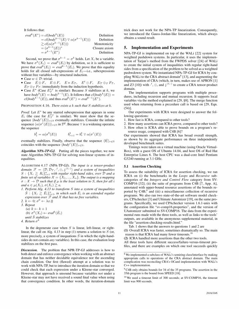
Figure 3: (a) Graphical representation of the linearized inequality given asEqn. (10); (b) finite-state machine for the valuations of all regular-languagepaths of Eqn. (10), i.e., (1t� d)(at� (bXc))∗T .

stant (much like ν was a stand-in for X in Eqn. (3)—see Ex. 2.1),we can create a “symbolically” left-linear system of inequalitiesover tensored weights:

ST : {Z & (1t� d)⊕T (Z ⊗T (at� (b⊗X ⊗ c)))}, (10)

where X = (t,·)(Z). The graphical representation of Eqn. (10) isshown in Fig. 3(a).

REMARK 4.8. The transformation of Eqn. (9) into Eqn. (10) isdifferent from the transformation used in Ex. 2.1 to turn Eqn. (2)into Eqn. (3) and then into Eqn. (4).• The transformation used in Ex. 2.1 leaves us with a left-linear in-

equality in which there is at most one variable in each summand.• The transformation of Eqn. (9) into Eqn. (10) produces a hybrid:

it is left-linear in Z, but X can appear in a summand that alsocontains a Z.

The advantage of this transformation will become apparent shortly.The transformation is formalized later in this section.

Applying Tarjan’s algorithm to Eqn. (10) gives us an expressionfor Z in terms of X (see Fig. 3(a)),

Z 7→ (1t� d)⊗T (at� (b⊗X ⊗ c))∗T , (11)

from which we obtain the following expression for X in terms ofX:

X 7→ (t,·)((1t� d)⊗T (at� (b⊗X ⊗ c))∗T ) .

Thus, the least solution of the system

S : {X & (t,·)((1t� d)⊗T (at� (b⊗X ⊗ c))∗T )}

coincides with the least solution of S. The significance of this se-quence of transformations is that in the system S, every occurrenceof a variable is “guarded” in the sense that it appears below a star. Ifwe let 〈κk : X → D〉k∈N denote the Kleene-iteration sequence forS, then we can define a “derived sequence” 〈βk〉k∈N in the iterationdomain D]:

βk def= α(at� (b⊗κk(X)⊗ c)) .

We observe that if the derived sequence converges (i.e., βk =βk−1 for some k), then so does the Kleene-interation sequence(κk+1(X) ≡ κk(X)). Moreover, convergence can be enforcedby applying the widening operator of the iteration domain to thederived sequence.

We now show how this process can be carried out for an arbi-trary system of inequalities over any number of variables. We beginby introducing a derived detensor-product operator that will aid inour symbolic manipulation of expressions.

DEFINITION 4.9. Let T = 〈D,DT , ·t,�, (t,·)〉 be a tensor-product domain. We define the detensor-product operator n :D ×DT → D as follows:

an p def= (t,·)((1t� a)⊗T p) .7

It is easy to show that for all a, b ∈ D and all p, q ∈ DT we have

an(p⊕T q) ≡ (an p)⊕ (an q)(a⊕ b)n p ≡ (an p)⊕ (bn p)

an(p⊗T (b� c)) ≡ bt⊗(an p)⊗ can 1T ≡ a

and if a ≡ b and p ≡T q then an p ≡ bn q. In the remainder ofthis section, we will assume that the following property holds (asit does for the CRA tensor-product domain): for all a ∈ D andp, q ∈ DT :

an(p⊗T q) ≡ (an p)n q .(Inclusion of this axiom makes 〈D,n〉 a right DT -module upto equivalence—i.e., n acts like scalar multiplication in vectorspaces, where the scalars are tensored weights and vectors areuntensored weights.)

Next, we define (tensored) extended regular expressions, whichcorrespond to the “expressions with symbolic constants” that weused in the construction of S above.

DEFINITION 4.10. Let T = 〈D,DT , ·t,�, (t,·)〉 be a tensor-product domain, and let X = {X1, ..., Xn} be a finite set ofvariables. A (tensored) extended regular expression over T andX is an expression generated by the following grammar:

E,F ∈ Ext(T ) ::= w ∈ D | Xi ∈ X | E⊕F | E⊗F| E∗ | EnET

ET , FT ∈ ExtT (T ) ::= (Et�F ) | ET ⊕T FT| ET ⊗T FT | E∗TT

An extended regular expression E over T is normal if for everysubexpression of E of the form EnET , ET is of the form F ∗TT .

For extended regular expressions E and F , we write E ' F todenote that for every function σ : X → D, we have σ(E) ≡ σ(F ).

DEFINITION 4.11. We say that an occurrence of a variable in a(tensored) extended regular expression is guarded if it appearsbelow a star. A variable with an unguarded occurrence is calledfree. Formally, for any (tensored) extended regular expression, itsset of free variables is defined as follows:

free(w)def= ∅

free(Xi)def= {Xi}

free(E⊕F )def= free(E) ∪ free(F )

free(E⊗F )def= free(E) ∪ free(F )

free(E∗)def= ∅

free(EnFT )def= free(E) ∪ freeT (FT )

freeT (E�F )def= free(E) ∪ free(F )

freeT (ET ⊕T FT )def= freeT (ET ) ∪ freeT (FT )

freeT (ET ⊗T FT )def= freeT (ET ) ∪ freeT (FT )

freeT (E∗TT )def= ∅

The next two propositions define the machinery that we willuse to successively eliminate all free variables from the right-handsides of a system of inequalities.• Prop. 4.12 shows that tensor-product can be used to rewrite a

right-hand side into X & F ⊕X nFT , which is “symbolically”left-linear in X .

7 Alternatively, we could have defined detensor-transpose in terms ofdetensor-product as (t,·)(p)

def= 1n p.

8 2016/10/6

• Alg. 4.13 successively invokes Prop. 4.12 to create X &F ⊕X nFT , which is then rewritten to X & F nFT ∗T . Theterm F nFT ∗T is then substituted into the other inequalities toeliminate all free occurrences of X .

This successive-elimination approach is related to Gauss-Jordan elimination, in that variables are successively eliminatedin some order. However, unlike in Gauss-Jordan elimination,only free occurrences of variables are eliminated—and thus ourmethod is only a partial elimination method.

The resulting equation system—all of whose variables appearunder ∗ or ∗T —is then solved by a successive-approximationmethod.

PROPOSITION 4.12. Let T = 〈D,DT , ·t,�, (t,·)〉 be a tensor-product domain, let X = {X1, ..., Xn} be a finite set of variables,and let E be a normal extended regular expression over T and X .For each variable X ∈ X , there exist extended regular expressionsF and FT such that1. E ' F ⊕ (X nFT ),2. F is normal, and3. X is not free in F .

Proof: By structural induction on E.• Case w ∈ D: we have w ' w⊕ (X n 0T )• Case X: we have X ' 0⊕ (X n 1T )• CaseXi ∈ X for someXi 6= X: we haveXi ' Xi⊕ (X n 0T )• Case E⊕E′: by the induction hypothesis, there is someF, FT , F

′, F ′T such that E ' F ⊕ (X nFT ) and E′ 'F ′⊕ (X nF ′T ) Then

E⊕E′ ' F ⊕ (X nFT )⊕F ′⊕ (X nF ′T )' (F ⊕F ′)⊕ (X n(FT ⊕T F ′T ))

• Case E⊗E′: by the induction hypothesis, there is someF, FT , F

′, F ′T such that E ' F ⊕ (X nFT ) and E′ 'F ′⊕ (X nF ′T ). Then:

E⊗E′ 'E⊗(F ′⊕ (X nF ′T ))' (E⊗F ′)⊕ (E⊗(X nF ′T ))' (E⊗F ′)⊕ (X n(F ′T ⊗T (Et� 1)))' ((F ⊕ (X nFT ))⊗F ′)⊕ (X n(F ′T ⊗T (Et� 1)))

' (F ⊗F ′)⊕ ((X nFT )⊗F ′)⊕ (X n(F ′T ⊗T (Et� 1)))

' (F ⊗F ′)⊕ (X n(FT ⊗T (1�F ′)))⊕ (X n(F ′T ⊗T (Et� 1)))

' (F ⊗F ′)⊕(X n

(FT ⊗T (1�F ′)

⊕T F ′T ⊗T (Et� 1)

))• Case E∗: we have E∗ ' E∗⊕ (X n 0T )• Case EnET : by the induction hypothesis, there is some F, FT

such that E ' F ⊕ (X nFT ). Then

EnET ' (F ⊕ (X nFT ))nET' (F nET )⊕ ((X nFT )nET )' (F nET )⊕ (X n(FT ⊗T ET ))

The last line of each case of the proof can be used to create arecursive function that implements the transformation.

ALGORITHM 4.13 (Free-Variable Elimination). The input is atensor-product domain T = 〈D,DT , ·t,�, (t,·)〉 and a systemof inequalities S : {Xi & Ri}ni=1 with regular right-hand sides,over D and a finite set of variables X = {X1, ..., Xn}. The outputis a system of inequalities S : {Xi & Ei}ni=1 where the right-handsides are normal extended regular expressions over T and X withno free variables, and such that the least solution to S coincideswith the least solution to S.

We transform S into S by eliminating variables one at a time,in a style reminiscent of Gauss-Jordan elimination. We use Sk :

{Xi & Ei,k}ni=1 to denote the system of inequalities after kelimination rounds (we take S0

def= S to be the original system of

equations, noting that each regular expressionRi from the originalsystem of equations is also an extended regular expression Ei,0).1. Repeat for each k = 1 to n:

(a) Rewrite Ek,k as Ek,k ' F ⊕ (Xk nFT ) (cf. Prop. 4.12).(b) Define Sk+1 : {Xi & Ei,k+1}ni=1 by:• Ek,k+1

def= F nF ∗TT

• For i 6= k, Ei,k+1 is obtained from Ei,k by replacingeach free occurrence of Xk with F nF ∗TT .

2. Return S def= Sn+1.

Correctness of Alg. 4.13. We would like to claim, “Given a sys-tem of inequalities S, Alg. 4.13 computes a system of inequalitiesS (of a particular form) such that the least solution of S coincideswith the least solution of S.” However, this statement does not hold,because a system of inequalities need not have a least solution overD (i.e., a solution µ to the system such that for every other solu-tion σ, µ(Xi) . σ(Xi) for all variables Xi). However, any quasiweight domain can be embedded into its completion, in which aleast solution always exists. (The least solution of a system of in-equalities in the completion is analogous to the combine-over-pathssolution of a dataflow-analysis problem.)

DEFINITION 4.14 (Completion of a quasi weight domain).Let D = 〈D,≡,⊕,⊗, ∗, 0, 1〉 be a quasi weight domain. Thecompletion of D, C(D) = 〈DC ,≡C ,⊕C ,⊗C , 0C , 1C〉,is the quasi weight domain in which the weightsDC = {A ∈ 2D : ∀a ∈ A∀b ∈ D.a ≡ b ⇒ b ∈ A} aresets of weights fromD (closed under equivalence), the equivalencerelation ≡C is equality, ⊕C is union, ⊗C is pointwise ⊗ (i.e.,A⊗C B

def= {a⊗ b : a ∈ A, b ∈ B}), A∗C def

=⋃

k∈NAn, 0C

def= ∅

is the empty set, and 1def= {1C} is the singleton set containing 1.

Completion extends to tensor-product domains in the natural way:for a tensor-product domain T = 〈D,DT , ·t,�, (t,·)〉 its com-pletion domain C(T ) is 〈C(D),C(DT ), ·tC ,�C ,

(t,·)C 〉 where

·tC , �C , and (t,·)C are defined pointwise.

Because the completion of a quasi weight domain D is a com-plete lattice and all of its operations are monotonic, any system ofinequalities over D has a unique least solution in C(D). It is thisleast solution that is preserved by the transformations in Alg. 4.13.

Having now formalized the correctness statement of Alg. 4.13,we will prove it. Let S : {Xi & Ri}ni=1 be a system of inequalitiesover D and a finite set of variables X = {X1, ..., Xn}.

Let σC : X → C(D) denote the least solution of S. Weargue that σC is the least solution to every intermediate system ofinequalities Sk by induction, working backward from Sn+1 = Sto S0 = S. For the induction step, we suppose that σC is the leastsolution to Sk+1 and prove that it is the least solution to Sk. RewriteEk,k as Ek,k ' F ⊕ (Xk nFT ) (cf. Prop. 4.12). Because σC isthe least solution to Sk+1, we must have

σC(Xk) = σC(Ek,k+1) = σC(F nF ∗TT ) .

9 2016/10/6

We then have:σC(Xk) = σC(F nF ∗TT )

= σC(F )nC σC(F ∗TT )= σC(F )nC σC(1C ⊕T (F ∗TT ⊗T FT ))= σC(F )nC(1C ⊕C(T )(σC(F ∗TT )⊗C(T ) σC(FT )))

=(σC(F )nC 1C)

⊕C (σC(F )nC(σC(F ∗TT )⊗C(T ) σC(FT )))

= σC(F )⊕C

(σC(F )nC

(σC(F ∗TT )⊗C(T ) σC(FT )

))= σC(F )⊕C

((σC(F )nC σC(F ∗TT )

)nC σC(FT )

)= σC(F )⊕C

((σC(F nF ∗TT )

)nC σC(FT )

)= σC(F )⊕C (σC(Xk)nC σC(FT ))= σC(F ⊕ (Xk nFT ))= σC(Ek,k)

and thus σC solves the constraint Xk & Ek,k.For every j 6= k, the right-hand-sides Ej,k and Ej,k+1 differ

only by substitution of F nF ∗TT for Xk, so because σC(Xk) =σC(F nF ∗TT ) we have σC(Ej,k) = σC(Ej,k+1). It follows fromthe fact that σC(Xj) & σC(Ej,k+1) that σC(Xj) & σC(Ej,k).We have thus shown that σC is a solution to Sk.

It remains to show that σC is the least solution to Sk. Supposethat σC is the least solution to Sk. We will prove that σC is asolution to Sk+1 so that (by virtue of σC being the least solutionto Sk+1 and σC being a solution to Sk+1, and the symmetricargument) σC and σC must coincide.

We begin by showing that σC solves the constraint Xk &Ek,k+1 (in fact, σC(Xk) = σC(Ek,k+1)). Observe that

σC(Ek,k+1) = σC(F n(FT )∗T )= σC(F )nC(σC(FT ))∗T

=⋃

j σC(F )nC(σC(FT ))j .

So to show that σC(Xk) ⊇ σC(Ek,k+1), it is sufficient to showthat for all j we have

σC(Xk) ⊇ σC(F )nC(σC(FT ))j . (12)

Note that because σC is the least solution to Sk, we have

σC(Xk) = σC(Ek,k) = σC(F )⊕C σC(Xk)nC σC(FT )

and thus

σC(Xk) ⊇ σC(F ) (13)σC(Xk) ⊇ σC(Xk)nC σC(FT ) (14)

We prove Eqn. (12) by induction on j.• Base case: immediate from Eqn. (13)• Induction step: Suppose that σC(Xk) ⊇ σC(F )nC(σC(FT ))j .

From Eqn. (14) and monotonicity of n, we have

σC(Xk) ⊇ σC(Xk)nC σC(FT )⊇ (σC(F )nC(σC(FT ))j)nC σC(FT )= σC(F )nC((σC(FT ))j ⊗C(T ) σC(FT ))= σC(F )nC(σC(FT ))j+1

So from the above we have that

σC(Xk) ⊇⋃j

σC(F )nC(σC(FT ))j = σC(Ek,k+1). (15)

We now need to show that σC(Xk) ⊆ σC(Ek,k+1). Let σ′C bethe map that sends Xk to σC(Ek,k+1), and every other variableXi to σC(Xi). It is easy to check that σ′C is a solution to Sk.By virtue of σC being the least solution to Sk, it follows thatσC(Xk) ⊆ σ′C(Xk) = σC(Ek,k+1). Thus, from Eqn. (15), wehave σC(Xk) = σC(Ek,k+1).

For every j 6= k, the right-hand-sides Ej,k and Ej,k+1 differonly by substitution of F nF ∗TT for Xk, so because σC(Xk) =

σC(F nF ∗TT ) we have σC(Ej,k) = σC(Ej,k+1). It follows fromthe fact that σC(Xj) & σC(Ej,k) that σC(Xj) & σC(Ej,k+1).We have thus shown that σC is a solution to Sk+1.

Because σC and σC are both solutions to Sk and Sk+1, σC isthe least solution to Sk, and σC is the least solution to Sk+1, wehave σC = σC , and σC is the least solution to Sk. This observationcompletes our argument that the least solution to S coincides withthe least solution to S.

Solving systems of inequalities with extended-regular-expressionright-hand sides. Let T = 〈D,DT , ·t,�, (t,·)〉 be a tensor-product domain, let X = {X1, ..., Xn} be a finite set of variables,and let S : {Xi & Ei}ni=1 be a system of inequalities in whicheach Ei is an extended regular expression over T and X with nofree variables.

Define a sequence of functions 〈σk : X → D〉k∈N as follows.The function σ0 is defined to be the constant 0 function. For eachk ≥ 1, define

σk(Xi)def= evalk(Ei)

whereevalk(w) = w

evalk(Xi) = σk−1(Xi)evalk(E⊕F ) = evalk(F )⊕ evalk(F )evalk(E⊗F ) = evalk(E)⊗ evalk(E)

evalk(E∗) = cl(bodyk(E)

)evalk(EnET ) = evalk(E)n evalkT (ET )evalkT (Et�F ) = evalkT (E)t� evalkT (F )

evalkT (ET ⊕T FT ) = evalkT (ET )⊕T evalkT (FT )evalkT (ET ⊗T FT ) = evalkT (ET )⊗T evalkT (FT )

evalkT (E∗TT ) = clT (bodykT (ET ))

andbodyk(E) = bodyk−1(E) O α(σk−1(E))

bodykT (ET ) = bodyk−1T (ET ) OT α(σk−1(ET )) .

We say that S stabilizes at k if for every subexpression of the formE∗ that appears in any Ei, we have

bodyk(E) = bodyk−1(E)

and for every subexpresssion of the form E∗TT that appears in anyEi, we have

bodykT (ET ) = bodyk−1T (ET ) .

THEOREM 4.15. If S stabilizes at k, then σk is a solution to S.

Proof: To show that σk is a solution to S, we must demonstrate thatσk(Xi) & σk(Ei) for all i. The essence of the argument is to showthat the following sequence of (in)equalities is valid:

σk(Xi) = evalk(Ei) & σk−1(Ei) = σk(Ei) .

The first equality in the sequence holds by the definition of σk. Themiddle inequality we prove by induction on Ei. We prove validityof the last equation by showing that the assumption that S stabilizesat k (i.e., the fact that bodyk(E) = bodyk−1(E) for every “loop-body” expression E) is sufficient to prove that σk−1 = σk.

First, we show that evalk(Ei) & σk−1(Ei) holds. We provethat this property holds for all sub-expressions of Ei by structuralinduction.• Case w ∈ D, Xj ∈ X : trivial.• Case E⊕F , E⊗F , EnET , Et�F , ET ⊕T FT ,ET ⊗T FT : from the induction hypothesis and monotonicity.• Case E∗ (Case E∗TT is similar): First, observe that by property 1

of the widening operator, we have

bodyk−1(E) O α(σk−1(E)) ≥] α(σk−1(E)) .

10 2016/10/6

It follows that:

evalk(E∗) = cl(bodyk(E)) Definition= cl(bodyk−1(E) O α(σk−1(E))) Definition& cl(α(σk−1(E))) Monotonicity= (σk−1(E))∗ Closure axiom= σk−1(E∗) Definition

Second, we prove that σk−1 = σk holds. Let Xi be a variable.We have σk(Xi) = evalk(Ei) by definition, so it is sufficient toprove that evalk(Ei) = evalk−1(Ei). We prove that this equalityholds for all closed sub-expressions of Ei—i.e., subexpressionswithout free variables—by structural induction.• Case w ∈ D: trivial.• Case E⊕F , E⊗F , EnET , Et�F , ET ⊕T FT ,ET ⊗T FT : immediately from the induction hypothesis.• Case E∗ (Case E∗TT is similar): Because S stabilizes at k, we

have bodyk(E) = bodyk−1(E). It follows that cl(bodyk(E)) =cl(bodyk−1(E)), and thus evalk(E∗) = evalk−1(E∗).

PROPOSITION 4.16. There exists a k such that S stabilizes at k.

Proof: Let E∗ be any starred subexpression that appears in someEi (the case for E∗TT is similar). We must show that the se-quence 〈bodyr(E)〉r∈N eventually stabilizes. Consider the infinitesequence 〈α(σr(E))〉r∈N inD]. Because O is a widening operator,the sequence

b]1 = α(σ0(E)) b]r+1 = b]r O α(σr(E))

eventually stabilizes. Finally, observe that the sequence 〈b]r〉r∈Ncoincides with the sequence 〈bodyr(E)〉r∈N.

Algorithm NPA-TP-GJ. Putting all the pieces together, we nowstate Algorithm NPA-TP-GJ for solving non-linear systems of in-equalities.

ALGORITHM 4.17 (NPA-TP-GJ). The input is a tensor-productdomain T = 〈D,DT , ·t,�, (t,·)〉 and a system of inequalitiesS : {Xi & Ri}ni=1 with regular right-hand sides, over D and afinite set of variables X = {X1, ..., Xn}. The output is a mappingσ : X → D such that if µ is the least solution to S, then for all iand a ∈ µ(Xi), σ(Xi) & a.1. Perform Alg. 4.13 to transform S into a system of inequalitiesS : {Xi & Ei}ni=1, in which each Ei is an extended regularexpression over T and X that has no free variables.

2. k ← 0; σ0 ← λx.03. Repeat

(a) k ← k + 1(b) σk(Xi)← evalk(Ei)

until S stabilizes4. Return σk

In the degenerate case when S is linear, left-linear, or right-linear, the call on Alg. 4.13 in step (1) returns a solution to S (or,more precisely, a system of inequations S in which the right-hand-sides do not contain any variables). In this case, the evaluation loopstabilizes on the first pass.

Discussion. The problem that NPR-TP-GJ addresses is how toboth detect and enforce convergence when working with an abstractdomain that has neither decidable equivalence nor the ascendingchain condition. Our first (flawed) attempt at a solution was towork with NPA-TP, but to introduce the iteration domain so that wecould check that each expression under a Kleene-star converged.However, that approach is unsound because variables not under aKleene-star may not have received a sound final value when usingthat convergence condition. In other words, the iteration-domain

trick does not work for the NPA-TP linearization. Consequently,we introduced the Gauss-Jordan-like linearization, which alwaysobtains a sound result.

5. Implementation and ExperimentsNPA-TP-GJ is implemented on top of the WALi [22] system forweighted pushdown systems. In particular, it uses the implemen-tation of Tarjan’s method from the FWPDS solver [24] of WALito create the initial system of inequalities with regular right-handsides from a specification of the problem to be solved as a weightedpushwdown system. We instantiated NPA-TP-GJ for ICRA by cou-pling WALi to the CRA abstract domain8 [13], and augmenting theimplementation of CRA (which, in turn, makes use of APRON [1]and Z3 [10]) with ·t, �, and (t,·) to create a CRA tensor-productdomain.

The implementation supports programs with multiple proce-dures, including recursion and mutual recursion. It supports localvariables via the method explained in [29, §8]. The merge functionused when returning from a prccedure call is based on [29, Eqn.(54)].

Our experiments with ICRA were designed to answer the fol-lowing questions:1. How fast is ICRA, compared to other tools?2. How many assertions can ICRA prove, compared to other tools?3. How often is ICRA able to prove bounds on a program’s re-

source usage, compared with C4B [6]?Our experiments showed that ICRA has broad overall strength,as shown by its aggregate performance on three independentlydeveloped benchmark suites.

Timings were taken on a virtual machine (using Oracle Virtual-Box), with a guest OS of Ubuntu 14.04, and host OS of Red HatEnterprise Linux 6. The host CPU was a dual-core Intel PentiumG3240 running at 3.1 GHz.

5.1 Assertion CheckingTo assess the suitability of ICRA for assertion checking, we ranICRA on (i) the benchmarks in the Loops and Recursive sub-categories of the Integers and Control Flow category from SV-COMP16 [32]; (ii) the suite of programs from C4B [7, App. A],annotated with upper-bound resource assertions of the bounds re-ported by C4B;9 and (iii) a miscellaneous collection of recursiveprograms. We also ran two state-of-the-art software model check-ers, CPAchecker [3] and Ultimate Automizer [19], on the same pro-grams. Specifically, we used CPAchecker version 1.6.1-unix withthe configuration file “sv-comp16.properties”, and the version ofUAutomizer submitted to SV-COMP16. The data from the experi-mental runs made with the three tools, as well as links to the tools’outputs, are available in the anonymous supplemental material, inthe file “assertion-checking-results.html.”

Tab. 1 shows that the answers to questions 1 and 2 are(1) Overall ICRA was faster, sometimes dramatically so. The mainreason is that ICRA had many fewer timeouts.10

(2) ICRA handled more assertions than the other two tools.All three tools have different success/failure-versus-timeout pro-files, and there are examples on which one tool succeeds quickly

8 We implemented a subclass of WALi’s semiring class/interface by makingappropriate calls to operations of the CRA abstract domain. The maincomplication was reconciling CRA’s OCaml implementation with WALi’sC++ implementation.9 C4B only obtains bounds for 34 of the 35 programs. The assertion in the35th program is the bound from SPEED [18].10 We used a timeout limit of 300 seconds; at SV-COMP16, the timeoutlimit was 900 seconds.

11 2016/10/6

Benchmark Total ICRA UAut. CPASuite #A Time #A Time #A Time #A

recursive 18/7 104.89 7/7 2,013.45 8/7 1,879.68 10/7rec.-simple 36/38 188.98 21/38 7,415.99 27/28 3,046.76 32/33Rec. (tot.) 54/45 293.87 28/45 9,429.44 35/35 4,926.44 42/40

loop-accel. 19/16 20.58 13/16 6,719.06 7/4 4,807.11 13/8loop-invgen 18/1 56.21 16/1 1,901.32 7/1 4,929.20 2/1loop-lit 15/1 323.43 12/1 2,744.02 4/1 2,758.87 6/1loop-new 8/0 6.40 7/0 2,151.40 1/0 1,874.28 3/0loops 34/32 190.53 19/31 4,091.96 20/19 4,605.55 27/27Loops (tot.) 94/50 597.15 67/49 17,607.76 39/25 18,975.01 51/37

C4B 35/0 31.68 29/0 6,182.25 1/0 8,072.61 2/0

Misc.-Rec. 10/4 325.23 9/4 525.06 8/4 344.45 7/1

Table 1: Column 2 shows the breakdown of programs into ones with validand invalid assertions. “X/Y” means that X is the number of programs con-taining valid assertions and Y is the number containing invalid assertions.The total number of programs is X + Y. The two columns for each toolshow the running time (in seconds) and the number of assertions proved. Incolumns 4, 6, and 8, “X/Y” means that (all) the valid assertions in X pro-grams were established, and (all) the invalid assertions in Y programs were(correctly) not established. A timeout is scored in neither category.

but the other tools time out. For instance, ICRA succeeds in prov-ing the assertion in the count_up_down_true-unreach-call_true-termination benchmark (shown below) in .55 seconds, whereasboth CPAchecker and UAutomizer time out:

int main() {unsigned int n = __VERIFIER_nondet_uint();unsigned int x=n, y=0;while(x>0) {x--; y++;

}__VERIFIER_assert(y==n);

}

In contrast, for the the underapprox_true-unreach-call1 benchmark(see below), both CPAchecker and UAutomizer were able to estab-lish the assertion, but ICRA was not.

int main(void) {unsigned int x = 0, y = 1;while (x < 6) {x++; y *= 2;

}__VERIFIER_assert(y % 3);

}

We were somewhat surprised that ICRA did not perform bet-ter on the recursive examples. However, it should be noted thatthe SV-COMP16 Recursive subcategory is probably not represen-tative, and many of the recursive benchmarks match up poorly withICRA’s current capabilities. In particular, many are merely copiesof the Fibonacci function with an assertion that the function com-putes a particular output value for a particular input. (There are35 variants of Fibonacci and 25 variants of the identity function.)These benchmarks are intended to be used with a software model-checker, which will unroll the recursion down to a sufficient depthto prove the assertion. In contrast, ICRA is designed to find invari-ants, and the invariant of the Fibonacci function is beyond our im-plementation’s current capabilities, although we are actively work-ing on enhanced recurrence-solving techniques that would handleit.

The test suite listed as Misc.-Rec. consists of a few newly-written recursive programs, as well as a few recursive programsdrawn from the test suite of the CRA static-analysis tool [13].

5.2 Applications in Resource-Bound AnalysisFor the experiments discussed in §5.1, the C4B benchmarks wereannotated with upper-bound resource assertions. We also explored

void perform(int n) {1. tick(7);2. if(*)3. tick(2);4. if(n>0) perform(n-1);5. tick(-3);}

void start(int n) {int flag = 1;while (flag > 0) {flag = 0;while (n > 0) {tick(1);n = n - 1;flag = 1;

} } }(a) (b)

Figure 4: (a) Recursive function used to illustrate upper and lower boundson resource usage. (b) The speed_pldi10_ex4.c benchmark from the C4Bsuite.

the use of ICRA for generating upper and lower bounds. (C4B itselfcan only establish upper bounds.)

The procedure in Fig. 4(a) illustrates the application of ICRA toresource-bound analysis. Statements of the form tick(k) representmanipulations of a resource such as memory or time, by consumingsome of the resource (if k is positive) or freeing some of theresource (if k is negative).

Given a program, ICRA can compute terms that upper-boundand lower-bound both the final resource usage and the high-watermark of resource usage.11 When computing bounds, it is usefulto treat positive and negative values of a program variable sepa-rately, so ICRA searches for bounds that include terms of the formmax(0, x) and max(0, y − x) (as in [7]), and we use the notation|[0, x]| and |[x, y]|, respectively, for such terms. For the functionperform, ICRA computes the following four bounds, each of whichis achieved by following paths of a particular form:

Bound Path (line numbers)final ≥ 4|[0, n]|+ 4 1→ 2→ 4→ perform(n-1) → 5final ≤ 6|[0, n]|+ 6 1→ 2→ 3→ 4→ perform(n-1) → 5hwm ≥ 7|[0, n]|+ 7 1→ 2→ 4→ perform(n-1) → 5hwm ≤ 9|[0, n]|+ 9 1→ 2→ 3→ 4→ perform(n-1) → 5

In the last two paths, each occurrence of tick(-3) encountered atline 5 has no effect on the value of the high-water mark.

On the C4B test suite, ICRA is able to generate upper boundson resource usage for 25 of the 35 programs, and nontrivial lowerbounds on resource usage for 25 of the programs (but not the sameset of 25). For 3 programs, ICRA obtains a tighter upper-boundthan C4B. For example, given the procedure shown in Fig. 4(b),ICRA generates the following bounds (the first of which improveson the C4B (upper) bound of final ≤ 1 + 2|[0, n]|):

final ≤ |[0, n]| final ≥ |[0, n]|

The source files and the outputs of the bounds-generation ex-periments on the C4B suite are available in the anonymous supple-mental material in the file “bounds-generation-results.html.”

6. Related WorkThe NPA-TP-GJ algorithm and its instantiation for ICRA rely heav-ily on prior work on CRA [13], NPA [12], and NPA-TP [29].• The NPA-TP-GJ algorithm adopts NPA-TP’s tensor-product op-

eration so that various terms in a non-linear inequality canbe rewritten into the “symbolically” left-linear form X &F ⊕X nFT , and then further rewritten as X & F nFT ∗T .• ICRA relies on the fact that the logic fragment that CRA employs

at loops to solve recurrence equations supports effective equiva-lence. That property—along with the widening performed during

11 The result of using ICRA for resource-bound analysis is only sound underthe assumption that every execution of the program in question terminatesfor all inputs.

12 2016/10/6

the body subroutine of eval, and the stabilization result given inThm. 4.15—ensures that ICRA will always terminate when it isapplied to a program that uses recursion.The elimination step in NPA-TP-GJ is related to Gauss-

Jordan elimination, in that variables are eliminated in some or-der. However, unlike in Gauss-Jordan elimination, variables areonly partially eliminated. (So-called “free variables” are elimi-nated, whereas variables that appear under ∗ or ∗T are not elim-inated.) Past work on Gauss-Jordan elimination for semirings orregular expressions includes Tarjan’s path-expression algorithm[33], Gondran & Minoux [15, §4.5], Rote [30, §4], Carré [8, §7],and Backhouse & Carré [2, §4]. The techniques developed in thepresent paper may open up the possibility of using those methods—or perhaps variants that only eliminate “free variables”—for inter-procedural program analysis.

Recently, a new iteration scheme was proposed by Meyer andMuskalla [26], called Munchausen Iteration (MI). MI is based onan iteration step that (a) works on a vector of expressions, and(b) substitutes the current approximant into itself. Both aspectshave some similarities with NPA-TP-GJ, but the substitution stepin MI is more aggressive. The benefit of MI is that, in principle,MI takes exponentially fewer rounds than NPA; however, Meyerand Muskalla indicate that MI is not yet an algorithm, “. . . so far,we do not know how to extract information from the [structuresthat represent answers].” Also, when the ascending-chain conditiondoes not hold, it is not clear how widening would be performed onthe symbolic structures that MI employs.

Although the performance of ICRA in the tool comparison re-ported in §5.1 is encouraging, it is important to note that ICRA isan invariant generator, while CPAchecker and UAutomizer are soft-ware model checkers. The standard trade-offs apply. CPAcheckerand UAutomizer are able to prove challenging program propertiesby employing abstraction refinement to tailor abstractions to theproperty at hand, but may refine abstractions indefinitely and failto terminate. ICRA can be used to compute rich program invariants(rather than just answer verification queries) but is not currentlyable to compute counter-example witnesses to assertion failures.(We illustrated one use of ICRA’s facility for invariant generationin §5.2 by employing ICRA to compute upper and lower bounds onresource usage.)

The success of compositional recurrence analysis is due to thepower of the iteration operator to summarize loops. There are anumber of related techniques for loop summarization [4, 17, 23]and abstract loop-acceleration [16, 21, 25] (which computes post-images of loops rather than summaries). Loop summarization inCRA is based on computing closed forms for recurrences satisfiedby loop bodies. ICRA harnesses the power of CRA’s loop summa-rization for computing summaries of recursive procedures by com-puting abstract transitive closures of tensored transition formulas;i.e., in ICRA, the input and output of the iteration operator are for-mulas that each have four distinct vocabularies.

7. ConclusionThis paper addresses the problem of creating a context-sensitiveinterprocedural version of CRA that handles loops and recursion—including non-linear recursion—in a uniform way. The methodpresented in the paper adopts, but adapts in significant ways, ideasused in the NPA-TP framework [29].

The presentation given in terms of the needed algebraic prop-erties has allowed us to state precisely the interface and propertiesrequired for NPA-TP-GJ to work. Although we currently have onlyone instantiation of NPA-TP-GJ—namely, ICRA—we believe thatthe algebraic formulation is a valuable contribution. We hope toapply NPA-TP-GJ to programs with loops that manipulate strings

or arrays, as well as to the analysis of probabilistic programs (forcomputing expectations of loops).

The results presented in the paper also offer a number of otheropportunities for future work. For instance, it would be valuable toknow whether some elimination orders for the Gauss-Jordan-likestep of ICRA are better than others (and why). We also have ideasabout how to incorporate additional methods for solving recurrenceequations in the interpretation of ∗ and ∗T . Finally, it would bedesirable to be able to perform witness tracing for ICRA.

References[1] APRON. APRON numerical abstract domain library. URL

http://apron.cri.ensmp.fr/library/.[2] R. Backhouse and B. Carré. Regular algebra applied to path-finding

problems. J. Inst. Maths. Applics., 15, 1975.[3] D. Beyer and M. Keremoglu. CPAchecker: A tool for configurable

software verification. In CAV, 2011.[4] S. Biallas, J. Brauer, A. King, and S. Kowalewski. Loop leaping with

closures. In SAS, 2012.[5] A. Bouajjani, J. Esparza, and O. Maler. Reachability analysis of

pushdown automata: Application to model checking. In CONCUR,1997.

[6] Q. Carbonneaux, J. Hoffmann, and Z. Shao. Compositional certifiedresource bounds. In PLDI, 2015.

[7] Q. Carbonneaux, J. Hoffmann, and Z. Shao. Compositional certifiedresource bounds (extended version). YALEU/DCS/TR-1505, YaleUniv., New Haven, CT, Apr. 2015.

[8] B. Carré. An algebra for network routing problems. J. Inst. Maths.Applics., 7, 1971.

[9] P. Cousot and R. Cousot. Abstract interpretation: A unified latticemodel for static analysis of programs by construction or approxima-tion of fixpoints. In POPL, 1977.

[10] L. de Moura and N. Bjørner. Z3: An efficient SMT solver. In TACAS,2008.

[11] J. Esparza, S. Kiefer, and M. Luttenberger. Newton’s method foromega-continuous semirings. In ICALP, 2008.

[12] J. Esparza, S. Kiefer, and M. Luttenberger. Newtonian program anal-ysis. J. ACM, 57(6), 2010.

[13] A. Farzan and Z. Kincaid. Compositional recurrence analysis. InFMCAD, 2015.

[14] A. Finkel, B.Willems, and P. Wolper. A direct symbolic approach tomodel checking pushdown systems. ENTCS, 9, 1997.

[15] M. Gondran and M. Minoux. Graphs, Dioids and Semirings: NewModels and Algorithms. Springer-Verlag, 2010.

[16] L. Gonnord and P. Schrammel. Abstract acceleration in linear relationanalysis. SCP, 93, 2014.

[17] S. Gulwani and F. Zuleger. The reachability-bound problem. In PLDI,2010.

[18] S. Gulwani, K. Mehra, and T. Chilimbi. SPEED: Precise and efficientstatic estimation of program computational complexity. In POPL,2009.

[19] M. Heizmann, J. Christ, D. Dietsch, E. Ermis, J. Hoenicke, M. Lin-denmann, A. Nutz, C. Schilling, and A. Podelski. Ultimate Automizerwith SMTInterpol (competition contribution). In TACAS, 2013.

[20] J. Hoffmann, K. Aehlig, and M. Hofmann. Multivariate amortizedresource analysis. TOPLAS., 34(3), 2012.

[21] B. Jeannet, P. Schrammel, and S. Sankaranarayanan. Abstract accel-eration of general linear loops. In POPL, 2014.

[22] N. Kidd, A. Lal, and T. Reps. WALi: TheWeighted Automaton Library, 2007. URLhttp://www.cs.wisc.edu/wpis/wpds/download.php.

[23] D. Kroening, N. Sharygina, S. Tonetta, A. Tsitovich, and C. Winter-steiger. Loop summarization using abstract transformers. In ATVA,2008.

13 2016/10/6

[24] A. Lal and T. Reps. Improving pushdown system model checking. InCAV, 2006.

[25] J. Leroux and G. Sutre. Accelerated data-flow analysis. In SAS, 2007.[26] R. Meyer and S. Muskalla. Munchausen itera-

tion. CoRR (arXiv), abs/1605.00422, 2016. URLhttp://arxiv.org/abs/1605.00422.

[27] T. Reps. Program analysis via graph reachability. IST, 40, 1998.[28] T. Reps, S. Schwoon, S. Jha, and D. Melski. Weighted pushdown

systems and their application to interprocedural dataflow analysis.SCP, 58, 2005.

[29] T. Reps, E. Turetsky, and P. Prabhu. Newtonian program analysis viatensor product. In POPL, 2016.

[30] G. Rote. Path problems in graphs. In Computational Graph Theory(Computing Supplementum 7). Springer-Verlag, 1990.

[31] M. Sharir and A. Pnueli. Two approaches to interprocedural dataflow analysis. In Program Flow Analysis: Theory and Applications.Prentice-Hall, 1981.

[32] SVCOMP16. 5th Int. competition on software verification (SV-COMP16), 2016. URL https://sv-comp.sosy-lab.org/2016/.

[33] R. Tarjan. Fast algorithms for solving path problems. J. ACM, 28(3):594–614, 1981.

14 2016/10/6