compsci 314 fc data communications fundamentals… · from application development, data...
TRANSCRIPT

7/20/2015 COMPSCI 314 S2C 2014 Ulrich Speidel 2
A bit about myself• I'm a physicst by training and didn't "become" a computer
scientist until my PhD
• Have taught in this department since 2000
• Have been involved in a wide variety of courses ranging from application development, data communication, Internet programming and introductory programming to computer architecture
• I'm quite an approachable person & just because I happen to have my door closed in 303S.594, it doesn't mean I'm trying to hide from you
2
Why I teach this course• My interest in electronic communication started as a teenager –
somewhat unusually with an aeronautical radiotelephone operator's certificate at age 16
• I then became interested in amateur radio, obtained a license and was active in Germany, Australia, and later in New Zealand
• Became involved quite heavily in packet radio (a kind of amateur radio predecessor of Wi‐Fi)
• Have since worked with all layers of the communication stack –from the physical layer (cable, radio, fibre…) to the applications (web) in both theory and practice
7/20/2015 COMPSCI 314 S2C 2014 Ulrich Speidel 3

Course structure
• Week 1‐4: Technical foundations and limits of data communication: channels, signals, codesLecturer: Ulrich Speidel
• Week 5‐8: Nevil Brownlee
• Week 9‐12: Aniket Mahanti
7/20/2015 COMPSCI 314 S2C 2014 Ulrich Speidel 4

Office hours
• Open door policy in 303S.594
• If you want an appointment, contact me on [email protected]
7/20/2015 COMPSCI 314 S2C 2014 Ulrich Speidel 5
7/20/2015 COMPSCI 314 S2C 2014 Ulrich Speidel 6
Assignments and Test
• I will set one assignment, due at 12:00 noon, Monday 10 August 2015
• Nevil and Aniket will also set one assignment each
• The mid‐semester test will be held during lecture time on September 18, 2015
7/20/2015 COMPSCI 314 S2C 2014 Ulrich Speidel 7
Communication with me• Don't be shy to approach me! Here's how to get a meaningful answer quickly…
• Put "COMPSCI314" in the subject of your e‐mail on a question that relates to COMPSCI314 – or risk being mistaken for a 280 student!
• Try to be as concise as possible in your question. It doesn't need to be as short as a text message. It helps if you refer to slide numbers, assignment questions, etc.
• I may anonymise your question and cc the rest of the class into my answer if I think it's of interest to others. Check and keep your class e‐mail – it'll often already contain the answer you're looking for.
• Note that around assignment due dates, tests and exams, I often get lots of questions by e‐mail. Checking your past class e‐mail is often a faster way to get an answer!
• Get in early and don't wait to the last minute if you need help.
7
7/20/2015 COMPSCI 314 S2C 2014 Ulrich Speidel 8
Other things
• I expect you to read your Computer Science e‐mail regularly (i.e., at least once a day)
• Announcements made via e‐mail are expected to be known to you 24 hours after they have been made
• Please see our tutor first if you have questions

7/20/2015 COMPSCI 314 S2C 2014 Ulrich Speidel 9
Our textbook
• “Computer Networking: A Top‐Down Approach”, 5th or 6th edition, by J.F. Kurose and K.W. Ross, Pearson Education
• Won't use this textbook in my part, but you might want to get it now for Nevil's & Aniket's parts
7/20/2015 COMPSCI 314 S2C 2014 Ulrich Speidel 10
What I'll cover – what you'll learn
• Theme 1: Physical foundations of data communications
• Data can travel across many media: cables, radio links – and each medium has its own special properties
• You'll learn about signals and the way we can express them in the physical world: electrical, optical, radio, …
• You'll develop an understanding of concepts such as latency, bandwidth, noise, bit rates, baud rates, and bit error rates, and how they relate to each other
7/20/2015 COMPSCI 314 S2C 2014 Ulrich Speidel 11
What I'll cover – what you'll learn
• Theme 2: Channels and codes
• In this theme, we'll learn about the characteristics of different channels and how we can package data for transport, so it gets to the receiver with as few errors and as little resource use as possible
• You'll develop an understanding of different channel types, where you'll likely to encounter them, and how information is coded and handled to deal with the requirements of each channel
Week 1
• Lecture 1: What's a signal? Electrical and optical signals
• Lecture 2: Radio signals, signal propagation, decibels
• Lecture 3: Satellite communication, communication channels and Fourier analysis, the concept of bandwidth
7/20/2015 COMPSCI 314 S2C 2014 Ulrich Speidel 12
Lecture 1
• What is a signal?
• Electrical signals
• Optical signals
7/20/2015 COMPSCI 314 S2C 2014 Ulrich Speidel 13
7/20/2015 COMPSCI 314 S2C 2014 Ulrich Speidel 14
Signals ‐ generally
“Potential”:
…could be the brightness of the light in an optical fibre…could be the voltage in an electric conductor…or, the level of water in a tank!

7/20/2015 COMPSCI 314 S2C 2014 Ulrich Speidel 15
Potential
difference in potential
Can define this differenceas “positive”(left tank hashigher water level than right tank, i.e., water will flow to the right)
7/20/2015 COMPSCI 314 S2C 2014 Ulrich Speidel 16
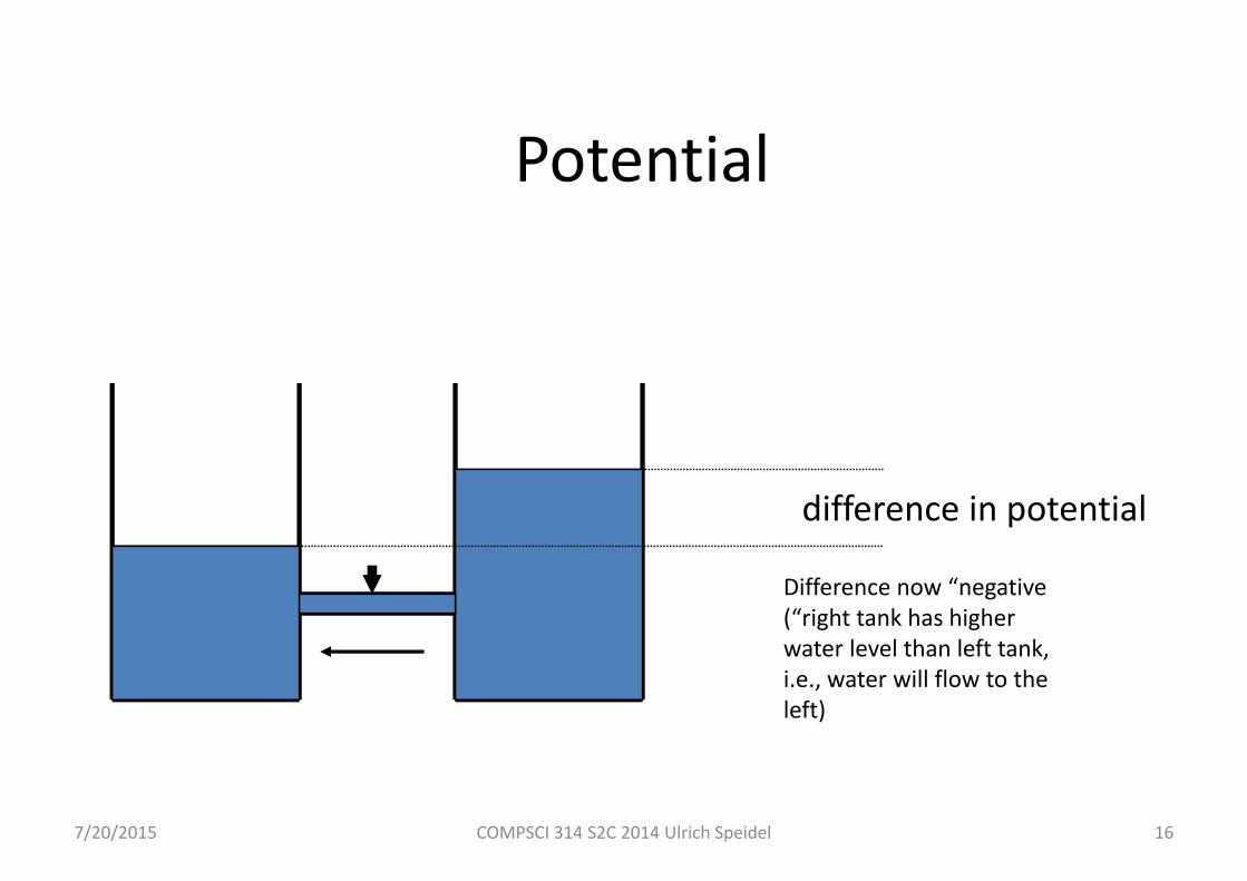
Potential
difference in potential
Difference now “negative(“right tank has higher water level than left tank, i.e., water will flow to the left)

7/20/2015 COMPSCI 314 S2C 2014 Ulrich Speidel 17
Potential
no difference in potential
No difference (“equipotential state” or“equilibrium”) meansno water will flow.Note that this state ispossible for arbitrary fill levels

7/20/2015 COMPSCI 314 S2C 2014 Ulrich Speidel 18
Potential and electrical signals
• Think about electrical conductors as water tanks withwater in them, with the water molecules being electrons
• Introducing signals means changing the water levelsin one or more of the tanks – pressure on valves or flowinto other tanks results
• The water pressure (potential) is the voltage
• The water flow (litres per second) is the current

Power• Water that flows through a device such as a turbine can do work for us, e.g., generate
energy. In physics, (the ability to perform) work and energy are the same.
• To perform work, we need both water pressure (voltage) and water flow (current).
• Current across a load such as a turbine can only perform work if it is driven by pressure.
• The amount of energy that can be created in a given amount of time is therefore proportional to the square of the water pressure (or square of the voltage)
• The amount of energy that can be transferred between systems per second is known as power and is measured in watts.
7/20/2015 COMPSCI 314 S2C 2014 Ulrich Speidel 19

7/20/2015 COMPSCI 314 S2C 2014 Ulrich Speidel 20
Types of (electrical) signals
Analog signals: potential changes continuously with time
• In communication, we often use analog signals that are limited in amplitude (certain minimal and maximal voltagesand/or currents are not exceeded) and that alternate betweenpositive and negative voltages/currents• Such signals may be thought of as the superposition of aamplitudes, frequencies, and phases of sinusoidal signals(Fourier theorem)• we’ll come back to that in a moment!
7/20/2015 COMPSCI 314 S2C 2014 Ulrich Speidel 21
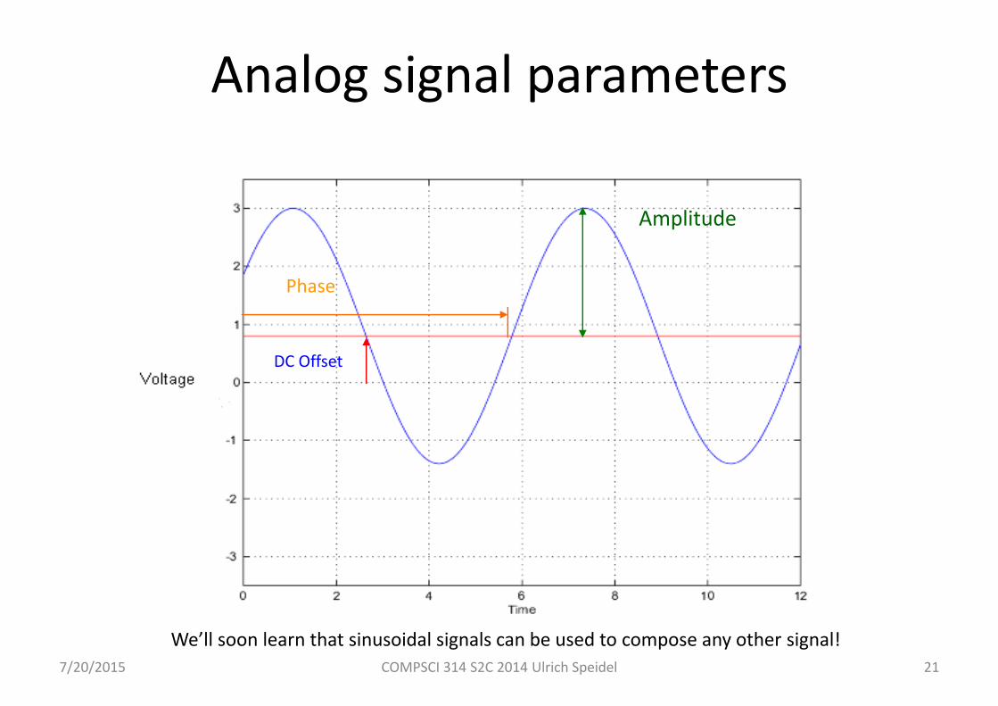
Analog signal parameters
We’ll soon learn that sinusoidal signals can be used to compose any other signal!
Amplitude
Phase
DC Offset
7/20/2015 COMPSCI 314 S2C 2014 Ulrich Speidel 22
Digital signals
• Digital signals are a special case of analog signals
• Ideally, they only have two discrete states, 0 and 1
• These may be expressed, e.g., as two different voltage levels or light intensities
• Transitions between 0 and 1 and vice versa are in theory instantaneous. That is, a digital system should never be in an “inbetween” state
• In practice, this is not possible. This fact causes a lot of problems!
7/20/2015 COMPSCI 314 S2C 2014 Ulrich Speidel 23
Digital vs. analog signals
• Both digital and analog signals can be used to convey information
• Analog signals are used for: conventional telephone, some older mobile phones, conventional radio and TV, as auxiliary carriers for some digital communication
• Digital signals are used for: data communication, including most mobile phones and digital radio/TV
7/20/2015 COMPSCI 314 S2C 2014 Ulrich Speidel 24
Digital vs. analog signals (II)
• Analog signal communication does not necessarily require a computer or digital logic!
• Analog signal communication cannot separate signal from noise
• Digital signal communication requires some sort of digital processor (more effort)
• Digital signal communication can separate signal from noise

7/20/2015 COMPSCI 314 S2C 2014 Ulrich Speidel 25
Transmission media
Both analog and digital signals can be communicated via the following media
• electrical conductors (coax, twinax, twisted pair, powerline, etc.)• optical fibre• air (i.e., radio, laser, smoke signals,…)
Let’s look closer at these three categories
7/20/2015 COMPSCI 314 S2C 2014 Ulrich Speidel 26
Electrical conductors (cable)
• Generally made from copper• Traditional cable form for data communication is coaxial cable (coax)
• Present‐day standard for Ethernet is “twisted pair”• Other cable forms are used (powerline, parallel cable, RS‐232 cable, etc.)

7/20/2015 COMPSCI 314 S2C 2014 Ulrich Speidel 27
Coax cables
• Inner conductor made of copper
• Plastic or foam insulation between inner core and shield
• Shield is copper mesh and/or tinfoil
• Outside insulation

7/20/2015 COMPSCI 314 S2C 2014 Ulrich Speidel 28
Coax cables (II)
• Ratio of diameters is important (impedance)• Overall diameter is important: the larger, the lower the losses (signal degradation over distance)
• Signal travels on inside conductor – outer conductor is grounded
• Cable does not radiate because the shield shields the inner conductor. Similarly, coax cables don’t pick up interfering signals for that reason.
7/20/2015 COMPSCI 314 S2C 2014 Ulrich Speidel 29
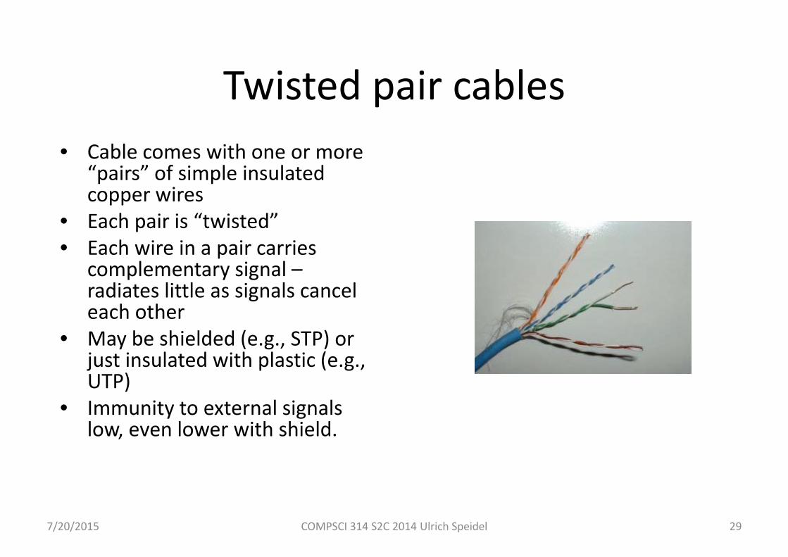
Twisted pair cables• Cable comes with one or more
“pairs” of simple insulated copper wires
• Each pair is “twisted”• Each wire in a pair carries
complementary signal –radiates little as signals cancel each other
• May be shielded (e.g., STP) or just insulated with plastic (e.g., UTP)
• Immunity to external signals low, even lower with shield.
7/20/2015 COMPSCI 314 S2C 2014 Ulrich Speidel 30
Optical fibre
• Made from glass or plastic• Cheap• Can be run for several km without amplifiers• More difficult to connect than copper wiring• Still an emerging technology!
7/20/2015 COMPSCI 314 S2C 2014 Ulrich Speidel 31
Optical fibre (II)
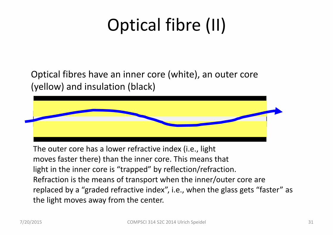
Optical fibres have an inner core (white), an outer core(yellow) and insulation (black)
The outer core has a lower refractive index (i.e., light moves faster there) than the inner core. This means thatlight in the inner core is “trapped” by reflection/refraction.Refraction is the means of transport when the inner/outer core are replaced by a “graded refractive index”, i.e., when the glass gets “faster” as the light moves away from the center.

7/20/2015 COMPSCI 314 S2C 2014 Ulrich Speidel 32
Optical fibre (III) ‐multimodeWe can send more than one light ray down a fibre by choosing different angles of incidence at the start
A fibre used in this way is called a “multimode fibre”. Multimode fibres are usually often for short distances only because it gets a bit difficult to keep the rays apart.Graded‐index fibre is best for this job.
Another way to put more information through a fibre is to send light in different colours (wavelength multiplexing).
7/20/2015 COMPSCI 314 S2C 2014 Ulrich Speidel 33
Optical fibre (IV)
• Used in most undersea cables and long distance overland cables because it’s so cheap
• When cables are laid, they usually contain several pairs of fibres (fibres come in pairs – one fibre for each direction of communication)
• Distances up to 40 km can be bridged without the need for repeaters
• Fibre repeaters are very expensive
• Fascinating read from Wired Magazine on submarine cables:
http://www.wired.com/wired/archive/4.12/ffglass.html

Lecture 2
• Radio signals
• Signal propagation
• Decibels
7/20/2015 COMPSCI 314 S2C 2014 Ulrich Speidel 34
7/20/2015 COMPSCI 314 S2C 2014 Ulrich Speidel 35
Wireless (aka “radio”)
• Big topic!• Traditionally used for overland phone circuits (analog)
• Now increasingly used in digital low power/short range applications: cellphones, Bluetooth, 802.11 WiFi, WiMax, 3G/4G/LTE, etc.
7/20/2015 COMPSCI 314 S2C 2014 Ulrich Speidel 36
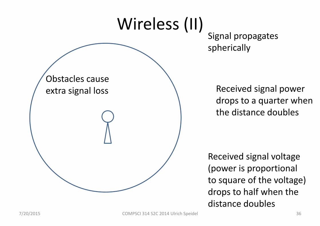
Wireless (II)Signal propagatesspherically
Received signal powerdrops to a quarter whenthe distance doubles
Received signal voltage(power is proportionalto square of the voltage)drops to half when thedistance doubles
Obstacles causeextra signal loss
7/20/2015 COMPSCI 314 S2C 2014 Ulrich Speidel 37
Wireless (III)
• Typical radio systems can live with a received signal power that is 1011 times smaller than the transmitted signal’s power
• Often this is not enough. Good antennas can help (e.g., dish for satellite communication)
7/20/2015 COMPSCI 314 S2C 2014 Ulrich Speidel 38
Wireless (IV) – how does it work?
• Think about an antenna as a conductor that has electrons pumpedinto and out of it at one end, with no connection at the other• This means the conductor gets charged and discharged in rapidcycles. Thus we have an electric field that gets built up and collapses in cycles all the time.• The electrons flowing in and out cause a magnetic field (electromagnet!). Thus we have a magnetic field that gets built up and collapses in cycles all the time.• The collapsing electric field away from the antenna causes a magnetic field there, and vice versa.
7/20/2015 COMPSCI 314 S2C 2014 Ulrich Speidel 39
Wireless (V) ‐ Propagation
• Radio signals propagate with the speed of light c(approx. 300,000,000 m/s in free space)
• If the cycle time is T, then a radio wave travels the distance λ = cT in the time that it completes one cycle. λ is called the “wavelength” of the wave
• f = 1/ T is called the “frequency” of the signal
7/20/2015 COMPSCI 314 S2C 2014 Ulrich Speidel 40
Decibels
• Used to compare voltage and power ratios• Two formulas• For two voltages V1 and V2 :
r (dB) = 20 log10 (V1/V2)• For two powers P1 and P2 :
r (dB) = 10 log10 (P1/P2)• A voltage ratio of 2:1 is approx. 6 dB• A power ratio of 2:1 is approx. 3 dB• You add ratios in dB – simpler that multiplying!• Remember that signal power is proportional to the square of the
voltages (hence the 20 and the 10 in the formulae above)
Decibels• Why decibels? They make large numbers (ratios) numbers that we can handle
easily
• Example: A transmitter sends a signal whose power is 10 watts. A distant receiver receives 1/1,000,000,000,000 of this power.
• An amplifier in the receiver then amplifies the signal power by a factor of 100
• Is that 0.0000000001 watts or 0.0000000001 watts, or even 0.000000000001 watts, or just 0.0000001 watts?
• If you’re hesitating, let’s use dB instead
7/20/2015 COMPSCI 314 S2C 2014 Ulrich Speidel 41
Decibels (continued)• Ratio between received and transmitted power:
1/1,000,000,000,000• Log to base 10 of that: ‐12• ‐12 times 10: ‐120 dB• Ratio between amplified and unamplified signal:
100• Log to base 10 of that: 2• 2 times 10: 20
• Add the dB figures (=multiply the ratios): ‐120 + 20 = ‐100• Convert back to a ratio: 10‐100/10=10‐10
• So, 10 watts * 10‐10 = 10‐9 watts = 0.000000001 watts
7/20/2015 COMPSCI 314 S2C 2014 Ulrich Speidel 42
Lost? Hopelessly log‐jammed?
• Scared of logarithms?
• Never seen them?
• Mentioned at school but seemed too hard?
Fear not – they’re actually quite easy once you’ve mastered a few very simple rules…
7/20/2015 COMPSCI 314 S2C 2014 Ulrich Speidel 43

Logarithm rule number 1
• Logarithms are the inverse of exponentials
• So, if x = yz, then logy x = z
• y is called the “base” of the logarithm (or, of the exponential function yz, for that matter)
• Examples: x = 256, y=2, z=8 x = 81, y = 3, z =4
7/20/2015 COMPSCI 314 S2C 2014 Ulrich Speidel 44

Logarithm rule number 2• Got the wrong base?
• E.g. you need log to base 10 but all your calculator can do is a log to base e (e=2.7182818284590452353602874…). A log to base e is often also just written as “ln”
• No problem. Just use the logarithm function you have and then divide by the
logarithm of the base you want:
• This works for any base, not just 10, and for any logarithm function you have at hand (as long as you use the same function for x and the base, of course)
7/20/2015 COMPSCI 314 S2C 2014 Ulrich Speidel 45
10lnlnlog10
xx
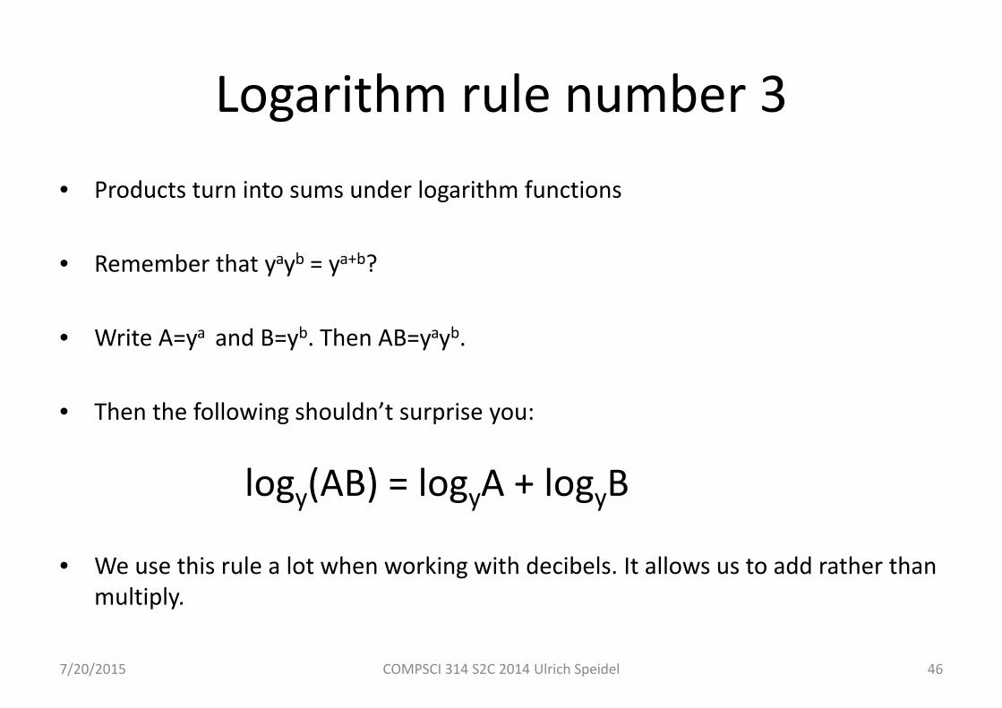
Logarithm rule number 3• Products turn into sums under logarithm functions
• Remember that yayb = ya+b?
• Write A=ya and B=yb. Then AB=yayb.
• Then the following shouldn’t surprise you:
logy(AB) = logyA + logyB
• We use this rule a lot when working with decibels. It allows us to add rather than multiply.
7/20/2015 COMPSCI 314 S2C 2014 Ulrich Speidel 46

Logarithm rule number 3b
• Ratios (quotients) turn into differences under logarithm functions
• This is natural extension of rule number 3
• So:logy(A/B) = logyA ‐ logyB
7/20/2015 COMPSCI 314 S2C 2014 Ulrich Speidel 47

Logarithm rule 3c• Powers (exponents) turn into factors under logarithm functions
• This is also a logical consequence of rule 3
• So:
logy (ab) = b logya
• Note: This rule lets us switch between the “power” formula and the “voltage” formula for decibels. Remember that power is proportional to the square of the voltage, hence we get a factor of 2… This turns the 10 into a 20.
• So: X decibels in power ratio are X decibels in voltage ratio. Always! But: The power ratio (when not quoted in dB) is always the square of its corresponding voltage ratio
7/20/2015 COMPSCI 314 S2C 2014 Ulrich Speidel 48
7/20/2015 COMPSCI 314 S2C 2014 Ulrich Speidel 49
Decibels: Examples
• The signal from a radio transmitter in free space drops by ?? dB when the distance to the transmitter doubles
• A signal amplifier with a gain of 40 dB produces a signal with an output amplitude that is ??? times higher than that of the input signal.
7/20/2015 COMPSCI 314 S2C 2014 Ulrich Speidel 50
Decibels: Examples
• The signal from a radio transmitter in free space drops by –6 dB when the distance to the transmitter doubles
• A signal amplifier with a gain of 40 dB produces a signal with an output amplitude that is ??? times higher than that of the input signal.

7/20/2015 COMPSCI 314 S2C 2014 Ulrich Speidel 51
Decibels: Examples
The signal from a radio transmitter in free space drops by –6 dB when the distance to the transmitter doubles
A signal amplifier with a gain of 40 dB produces a signal with an output amplitude that is 100 times higher than that of the input signal.
Using decibels to quote powers
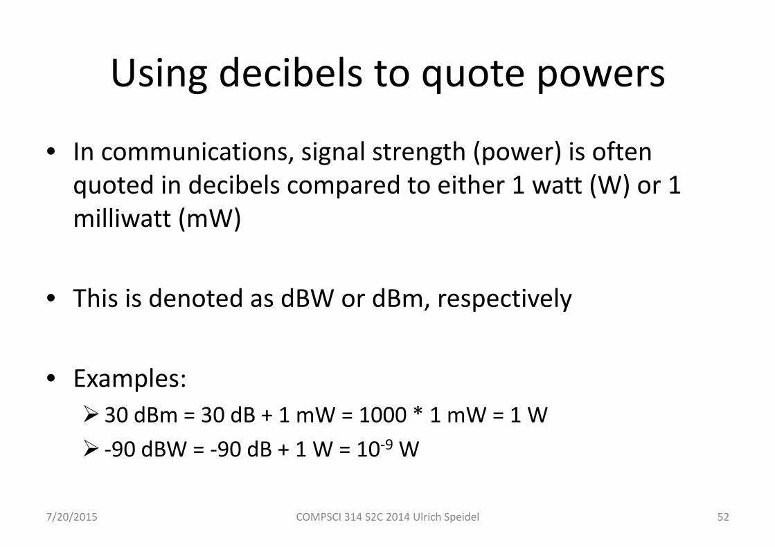
• In communications, signal strength (power) is often quoted in decibels compared to either 1 watt (W) or 1 milliwatt (mW)
• This is denoted as dBW or dBm, respectively
• Examples:30 dBm = 30 dB + 1 mW = 1000 * 1 mW = 1 W ‐90 dBW = ‐90 dB + 1 W = 10‐9 W
7/20/2015 COMPSCI 314 S2C 2014 Ulrich Speidel 52
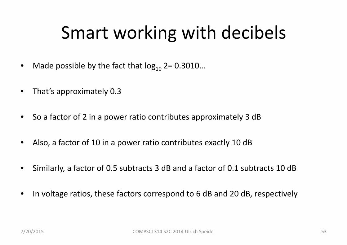
Smart working with decibels• Made possible by the fact that log10 2= 0.3010…
• That’s approximately 0.3
• So a factor of 2 in a power ratio contributes approximately 3 dB
• Also, a factor of 10 in a power ratio contributes exactly 10 dB
• Similarly, a factor of 0.5 subtracts 3 dB and a factor of 0.1 subtracts 10 dB
• In voltage ratios, these factors correspond to 6 dB and 20 dB, respectively
7/20/2015 COMPSCI 314 S2C 2014 Ulrich Speidel 53
Smart working with decibels
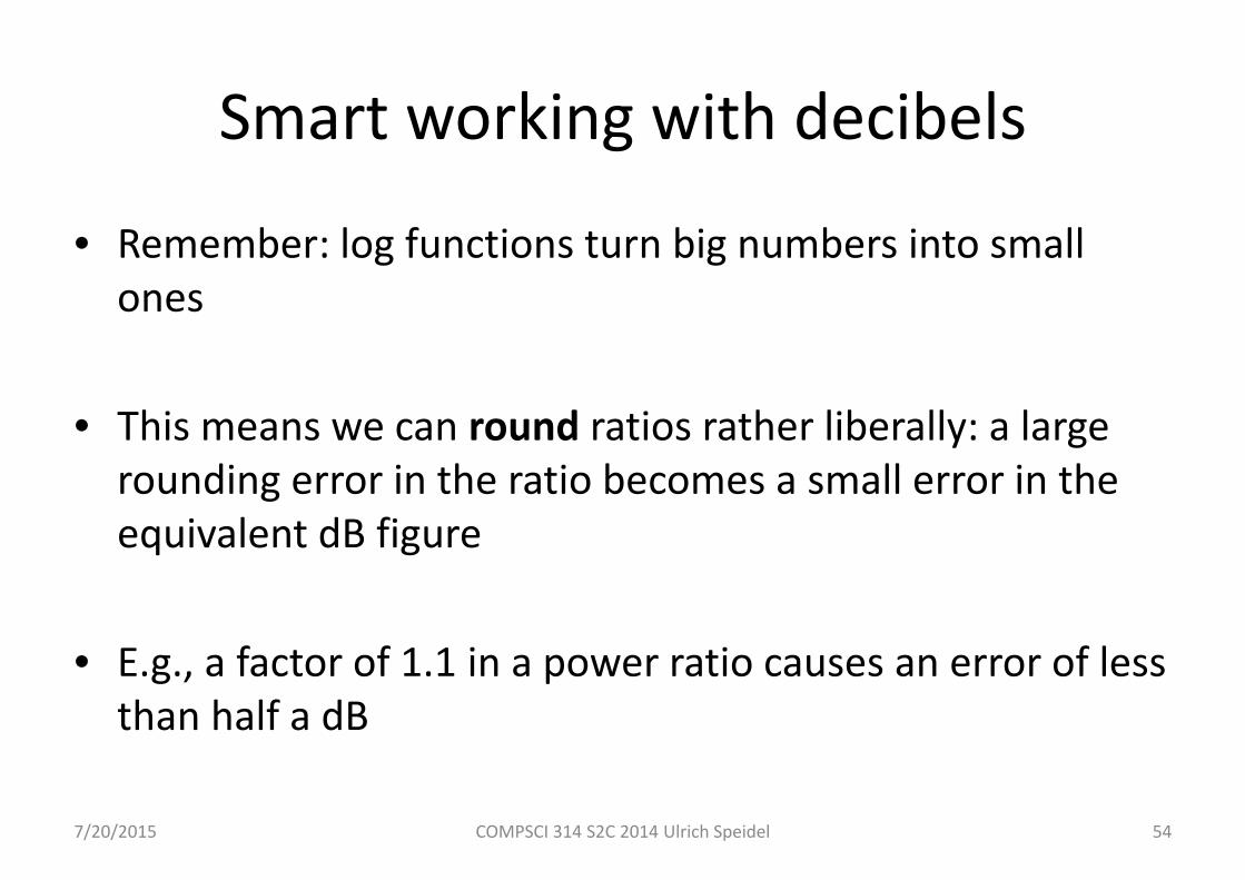
• Remember: log functions turn big numbers into small ones
• This means we can round ratios rather liberally: a large rounding error in the ratio becomes a small error in the equivalent dB figure
• E.g., a factor of 1.1 in a power ratio causes an error of less than half a dB
7/20/2015 COMPSCI 314 S2C 2014 Ulrich Speidel 54
Smart working with decibels
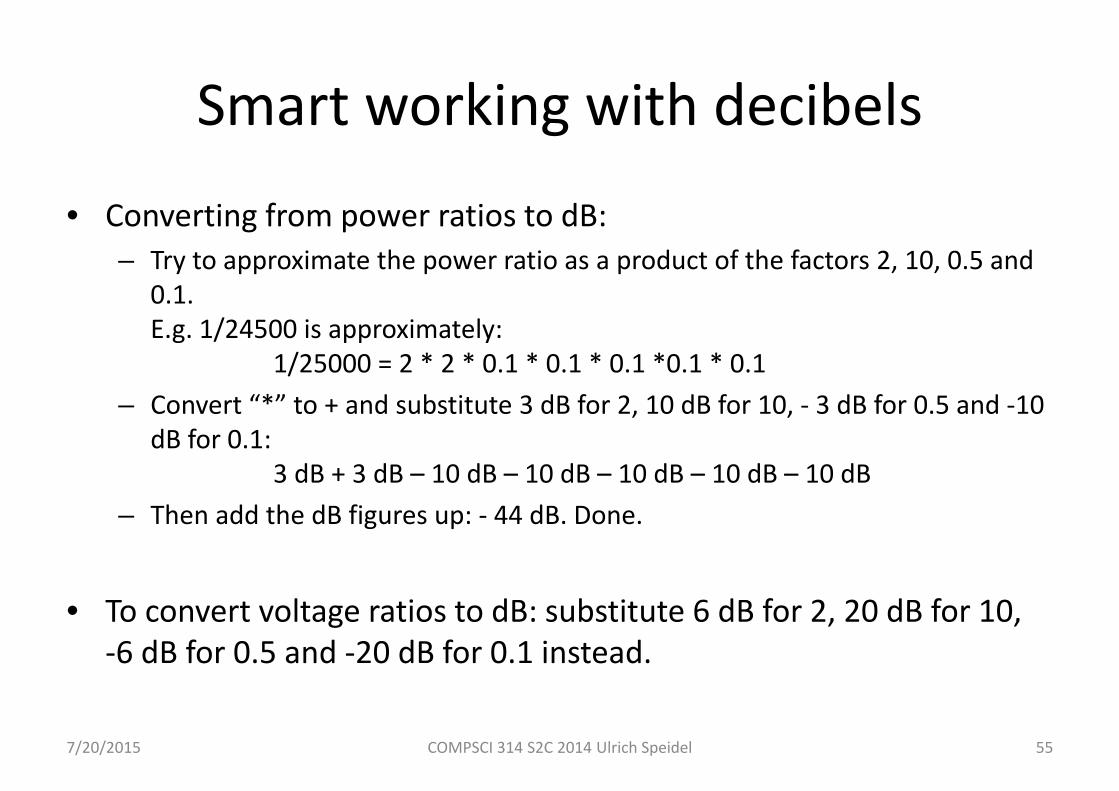
• Converting from power ratios to dB:– Try to approximate the power ratio as a product of the factors 2, 10, 0.5 and
0.1. E.g. 1/24500 is approximately:
1/25000 = 2 * 2 * 0.1 * 0.1 * 0.1 *0.1 * 0.1– Convert “*” to + and substitute 3 dB for 2, 10 dB for 10, ‐ 3 dB for 0.5 and ‐10
dB for 0.1:3 dB + 3 dB – 10 dB – 10 dB – 10 dB – 10 dB – 10 dB
– Then add the dB figures up: ‐ 44 dB. Done.
• To convert voltage ratios to dB: substitute 6 dB for 2, 20 dB for 10, ‐6 dB for 0.5 and ‐20 dB for 0.1 instead.
7/20/2015 COMPSCI 314 S2C 2014 Ulrich Speidel 55
Smart working with decibels
• To convert a dB figure into a power ratio:– Try to express the dB figure as a sum of 3 dB, 10 dB, ‐3 dB and – 10 dB.
E.g., 35 dB = 10 dB + 10 dB + 3 dB + 3 dB + 3 dB + 3 dB + 3 dB– Substitute 3 dB by a factor of 2, 10 dB by a factor of 10, ‐ 3 dB by a factor of
0.5, and ‐10 dB by a factor of 0.1:10 * 10 * 2 * 2 * 2 * 2 * 2
– Multiply them all together: 320
• For voltage ratios, use summands of 6 dB and 20 dB respectively. For added precision, allow yourself a single 3 dB or – 3dB term and multiply or divide by 1.4 (or 1.5 if you’re not too fussed)
7/20/2015 COMPSCI 314 S2C 2014 Ulrich Speidel 56
7/20/2015 COMPSCI 314 S2C 2014 Ulrich Speidel 57
Propagation in wire and fibre
• Similar concepts apply to signals propagating in wires and fibres. Light in particular is actually a radio wave, albeit with an extremely high frequency.
• λ is always quoted as the “vacuum” wavelength – this applies in particular to fibre optics!
• Signals in wire or fibre propagate at typically about 2/3rds of c,i.e., at about 200,000,000 m/s.
• Exact speed varies a bit depending on the actual media, typically 0.6...0.7 c.
• In fibre, the factor is 1/a where a is the refractive index of the fibre core.
• Losses in wire and fibre are not due to spreading, but due to attenuation in the material (light or electrical power is converted into heat).
Lecture 3
• Satellite communication
• Communication channels
• Fourier analysis
• Signals in the time domain and frequency domain (power spectra)
7/20/2015 COMPSCI 314 S2C 2014 Ulrich Speidel 58
7/20/2015 COMPSCI 314 S2C 2014 Ulrich Speidel 59
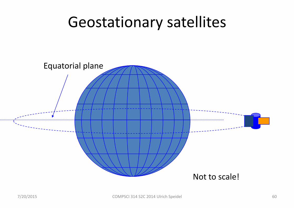
Geostationary satellites
• Also called “geosynchronous”• High circular orbit in the equatorial plane (35,786 km above the equator)
• Orbit the earth exactly once every siderial day (= the time the earth takes to rotate around its axis, this is slightly less than 24 hrs because the earth’s orbiting around the sun needs to be subtracted)
• Appear to be in the same spot in the sky 24hrs a day if viewed from the earth – easy to point a dish antenna at!
7/20/2015 COMPSCI 314 S2C 2014 Ulrich Speidel 60
Geostationary satellites
Not to scale!
Equatorial plane
Geostationary orbits
7/20/2015 COMPSCI 314 S2C 2014 Ulrich Speidel 61
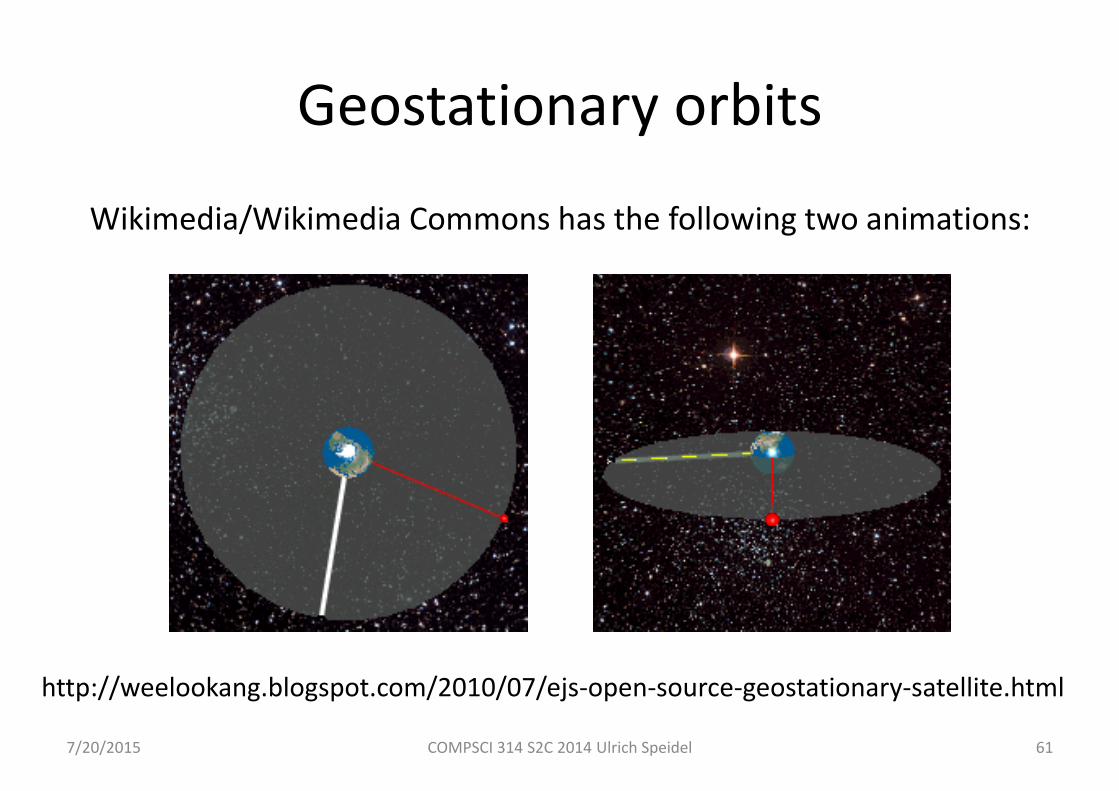
Wikimedia/Wikimedia Commons has the following two animations:
http://weelookang.blogspot.com/2010/07/ejs‐open‐source‐geostationary‐satellite.html
7/20/2015 COMPSCI 314 S2C 2014 Ulrich Speidel 62
Low/Medium‐Earth‐Orbit (LEO/MEO) satellites
• Orbital altitude less than that of geostationary satellites
• Don’t appear to be in the same spot
• Can be used to “cover” more territory
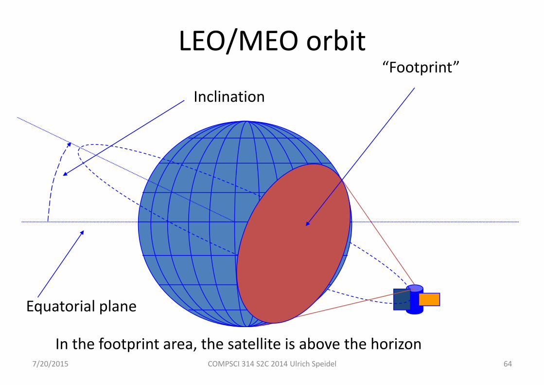
• Have an “inclination” (angle between orbital plane and equatorial plane)
• Inclination determines highest/lowest latitude that the satellite can “cover” (=not a good communication solution for polar regions such as Antarctica)
• Need to track the satellite with steerable antenna to achieve large bandwidths, but antennas tend to be smaller
• Examples: GPS, Iridium (LEO), O3b (MEO)

GEO & MEO ground station
7/20/2015 COMPSCI 314 S2C 2014 Ulrich Speidel 63
GEO antenna(fixed)
MEO antennas(steerable)
One MEO antenna(red arrow)tracks currentsatellite, otherantenna (green arrow)awaits rise ofnext satelliteover horizonto take over tracking
7/20/2015 COMPSCI 314 S2C 2014 Ulrich Speidel 64
LEO/MEO orbit“Footprint”
In the footprint area, the satellite is above the horizon
Equatorial plane
Inclination

7/20/2015 COMPSCI 314 S2C 2014 Ulrich Speidel 65
Satellite communication issues
• Latency can be much higher than for cable or fibre• Renting a transponder (satellite channel) can be much cheaper than
running a cable over hundreds or thousands of km• Most communication satellites used to be geostationary, but in
recent times LEO’s/MEO's (e.g., Iridium, GPS, O3b, etc.) have been used successfully (at least from a technical point of view)
• Satellites don’t require landowner approval but can be jammed easily unless spread‐spectrum technology is used
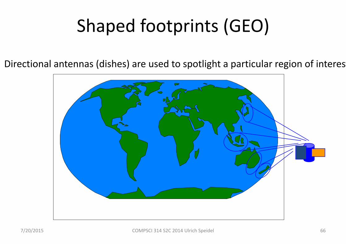
• Antennas can be used to “shape” footprints – deliver all your power into the area you want to cover
7/20/2015 COMPSCI 314 S2C 2014 Ulrich Speidel 66
Shaped footprints (GEO)
Directional antennas (dishes) are used to spotlight a particular region of interest
7/20/2015 COMPSCI 314 S2C 2014 Ulrich Speidel 67
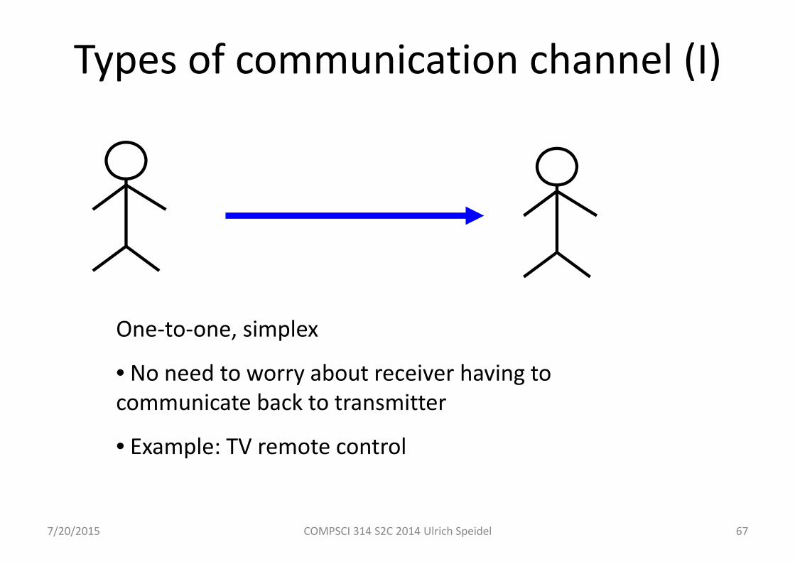
Types of communication channel (I)
One‐to‐one, simplex
• No need to worry about receiver having to communicate back to transmitter
• Example: TV remote control
7/20/2015 COMPSCI 314 S2C 2014 Ulrich Speidel 68
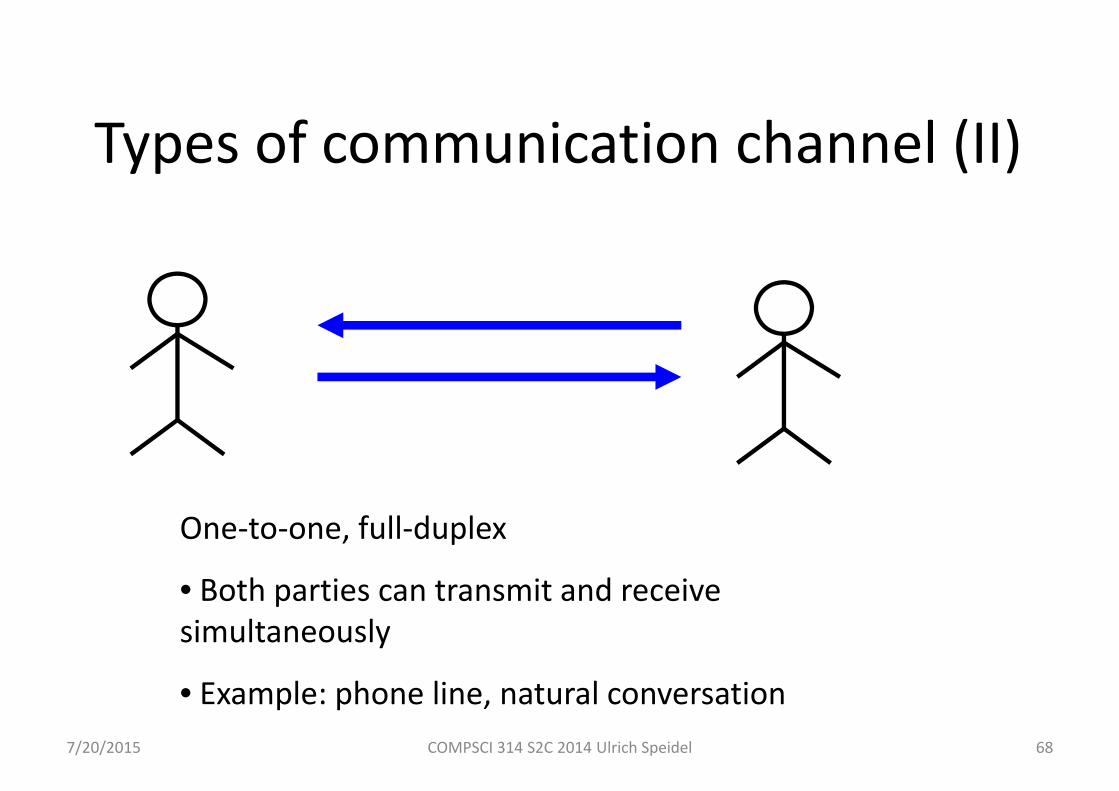
Types of communication channel (II)
One‐to‐one, full‐duplex
• Both parties can transmit and receive simultaneously
• Example: phone line, natural conversation
7/20/2015 COMPSCI 314 S2C 2014 Ulrich Speidel 69
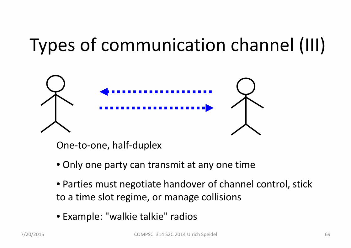
Types of communication channel (III)
One‐to‐one, half‐duplex
• Only one party can transmit at any one time
• Parties must negotiate handover of channel control, stick to a time slot regime, or manage collisions
• Example: "walkie talkie" radios
7/20/2015 COMPSCI 314 S2C 2014 Ulrich Speidel 70
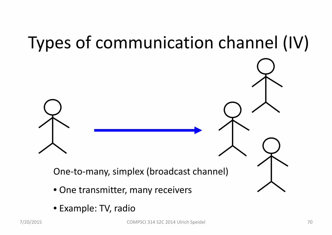
Types of communication channel (IV)
One‐to‐many, simplex (broadcast channel)
• One transmitter, many receivers
• Example: TV, radio
7/20/2015 COMPSCI 314 S2C 2014 Ulrich Speidel 71
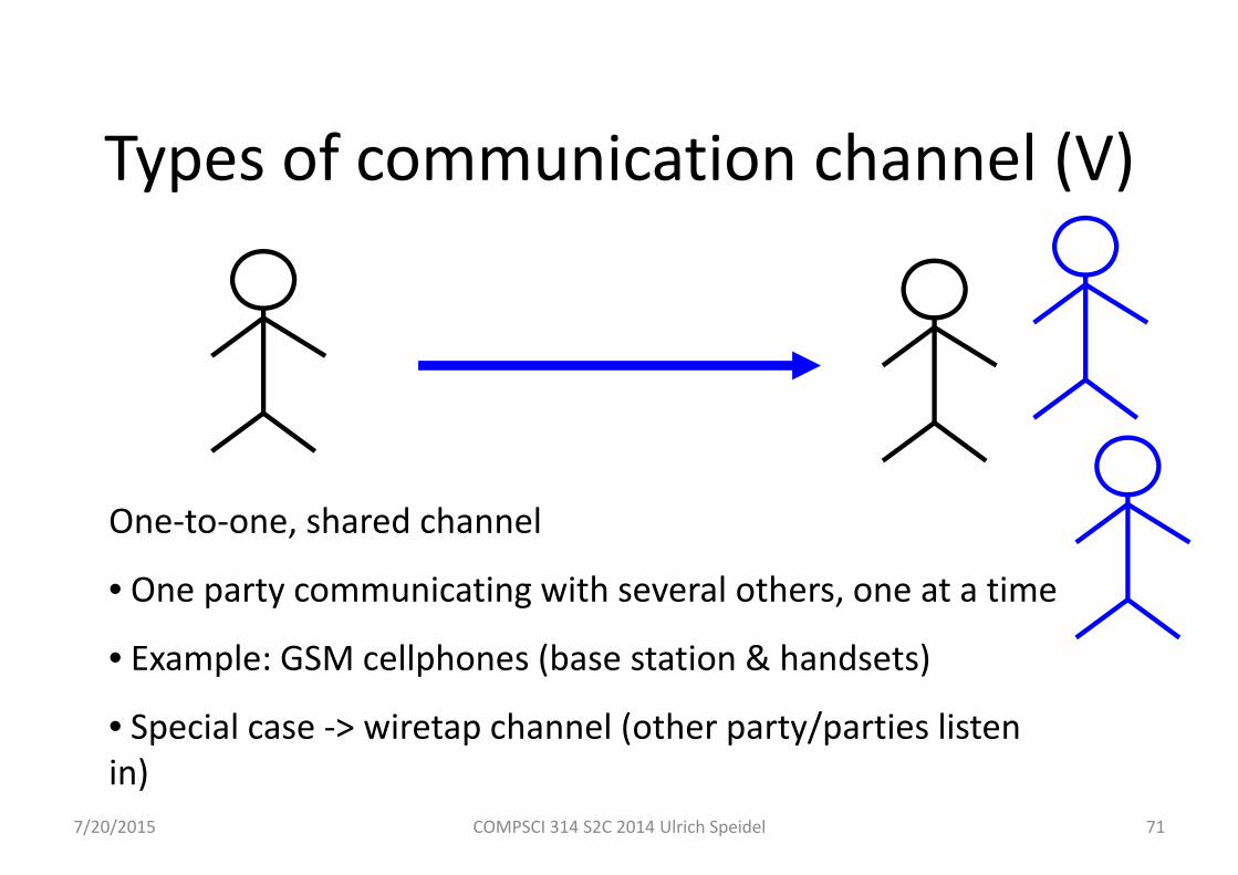
Types of communication channel (V)
One‐to‐one, shared channel
• One party communicating with several others, one at a time
• Example: GSM cellphones (base station & handsets)
• Special case ‐> wiretap channel (other party/parties listen in)
7/20/2015 COMPSCI 314 S2C 2014 Ulrich Speidel 72
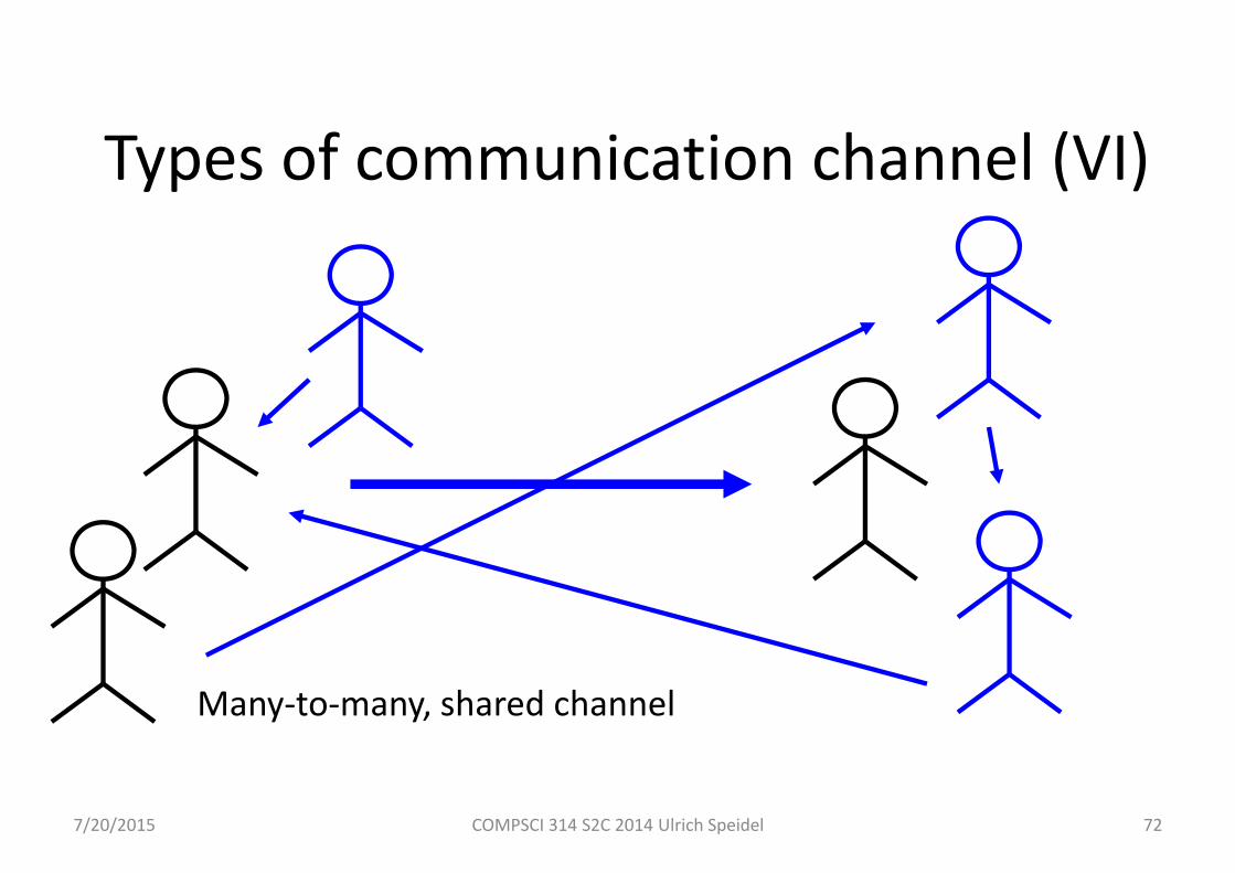
Types of communication channel (VI)
Many‐to‐many, shared channel
Notes on many‐to‐many channels
• Participants act as both transmitters and receivers
• Only one transmitter can access the channel at a time– participants must negotiate channel access, manage collisions, or stick to a timing scheme
• Not every receiver may be able to hear every transmitter
• Example: 802.11 WiFi
7/20/2015 COMPSCI 314 S2C 2014 Ulrich Speidel 73

7/20/2015 COMPSCI 314 S2C 2014 Ulrich Speidel 74
Channel type summary
• Each type of channel has its own characteristic
• Need to make adequate provisions for privacy/security, equal access, etc.
• There is no “one‐size‐fits‐all” solution that works for every type of channel/scenario
• You must judge what works best where
• Will return to channel types a little later once we've discussed modulation and noise
7/20/2015 COMPSCI 314 S2C 2014 Ulrich Speidel 75
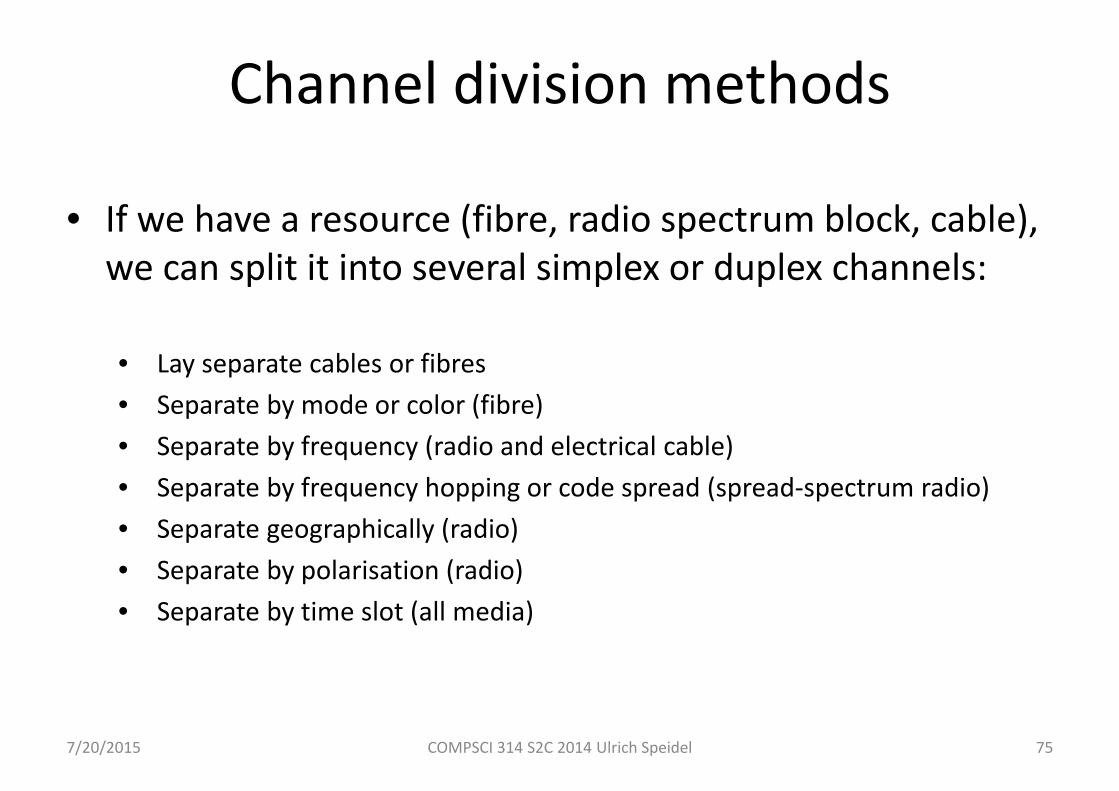
Channel division methods
• If we have a resource (fibre, radio spectrum block, cable), we can split it into several simplex or duplex channels:
• Lay separate cables or fibres• Separate by mode or color (fibre)• Separate by frequency (radio and electrical cable)• Separate by frequency hopping or code spread (spread‐spectrum radio)• Separate geographically (radio)• Separate by polarisation (radio)• Separate by time slot (all media)
Signals and information
• So far, we’ve talked about signals but have concentrated on how they can be sent between two physical locations
• We haven’t looked at what signal actually are, how we can describe them, and how we can get them to carry information for us.
• This is what we’ll do next. We start with looking at what makes up a signal.
7/20/2015 COMPSCI 314 S2C 2014 Ulrich Speidel 76
7/20/2015 COMPSCI 314 S2C 2014 Ulrich Speidel 77
Quick glossary to remember
• The frequency is the number of oscillation cycles per second, measured in hertz (Hz)
• The amplitude is the “height” of the signal (voltage), typically measured in volts (V)
• The power is always proportional to the square of a voltage. It’s measured in watts (W)
• The phase of a sine wave is a measure for how much the waveform is shifted to the left or right (i.e., along the time axis). It’s an angle, so it’s typically measured in degrees or radians.
7/20/2015 COMPSCI 314 S2C 2014 Ulrich Speidel 78
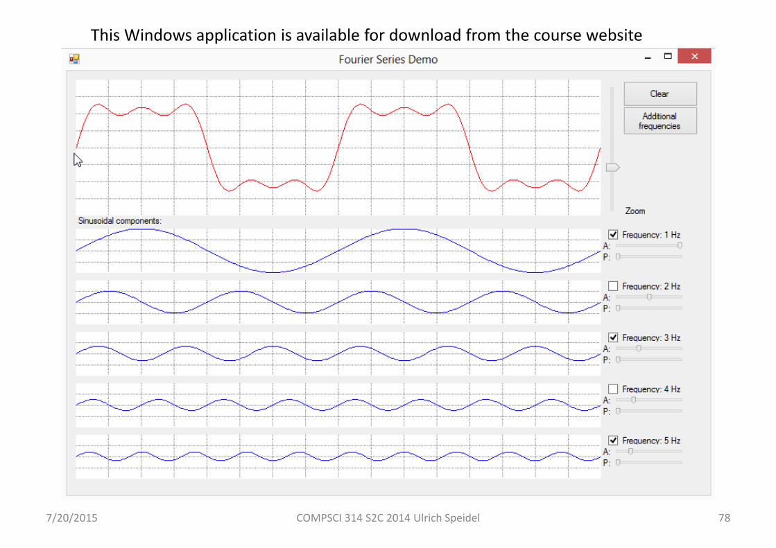
This Windows application is available for download from the course website
Fourier transforms / series
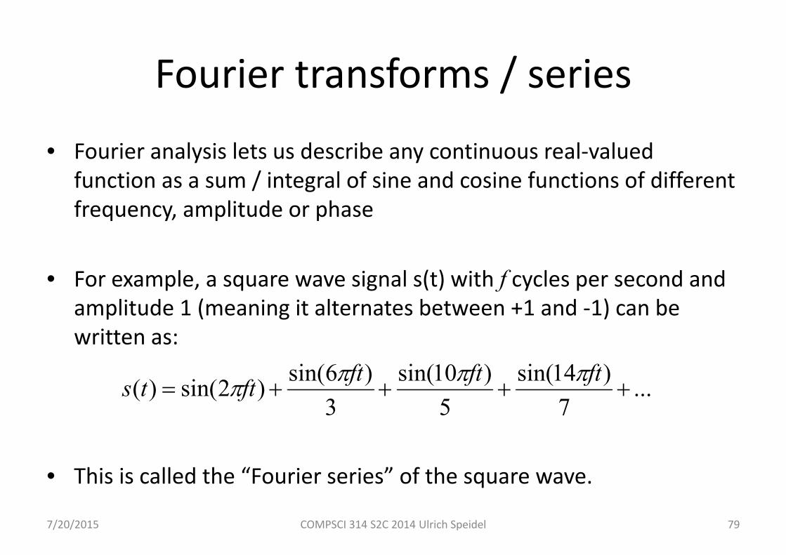
• Fourier analysis lets us describe any continuous real‐valued function as a sum / integral of sine and cosine functions of different frequency, amplitude or phase
• For example, a square wave signal s(t) with f cycles per second and amplitude 1 (meaning it alternates between +1 and ‐1) can be written as:
• This is called the “Fourier series” of the square wave.
7/20/2015 COMPSCI 314 S2C 2014 Ulrich Speidel 79
...7
)14sin(5
)10sin(3
)6sin()2sin()( ftftftftts

Implications of Fourier analysis• As a CS student, you'll know what a bit is: 0 or 1. A 0 is for low voltage level and 1 is for high voltage level (or vice
versa)
• Now think of the bit sequence ….1010101010101…
• That's a square wave
• Fourier analysis tells us that to make a perfect square wave, we need an infinite number of sine functions with (ultimately) infinitely high frequencies
• That isn't very practical. So any "real" square wave in a real computer is only an approximation. A 0 bit is "more or less low voltage" and a 1 bit is "more or less high voltage".
• So, real 0 and 1 bits don't actually exist. Yes, they did lie to you in stage 1 and 2. Sorry.
• Moreover, transitions between such approximated 0 and 1 bits are not instantaneous. The higher the frequencies we can include, the faster the transitions become.
7/20/2015 COMPSCI 314 S2C 2014 Ulrich Speidel 80
Fourier analysis and bandwidth
• The transition time between bits limits the number of different bits we can transmit per time unit (i.e., per second)– The faster we can transition between different bits, the more bits per second
we can transmit– The more frequencies we can include, the more bits per second we can
transmit
• The bandwidth of a communication channel is the difference between the highest and the lowest frequency it can carry – the width of the frequency band in which the communication takes place
• bandwidth ~= (potential) bit rate
7/20/2015 COMPSCI 314 S2C 2014 Ulrich Speidel 81
Fourier notes I
• Real bit streams we want to communicate aren't perfect square waves but look "more realistic" (limited in time and with 0's and 1's lumping together)
• The Fourier analysis in such cases becomes a little bit more complex
• But the principle remains: Transition edges between different bits get sharper with increasing bandwidth!
7/20/2015 COMPSCI 314 S2C 2014 Ulrich Speidel 82
Fourier notes II• If the lowest frequency in our band is 0 Hz, we call the signal in the band the
baseband signal. – A simple bit stream with low/high voltage levels for 0/1 bits is always a baseband
signal
• Modulation (see next lecture) allows us to shift a baseband signal into a frequency band whose lowest frequency is (usually much) larger than 0 Hz
• You may have heard of "radio spectrum auctions" where mobile phone companies get to buy bands in the radio spectrum
– As the spectrum is limited, these bands are valuable: The more bandwidth a company can win, the more customers it can serve and the better the service it can offer
7/20/2015 COMPSCI 314 S2C 2014 Ulrich Speidel 83
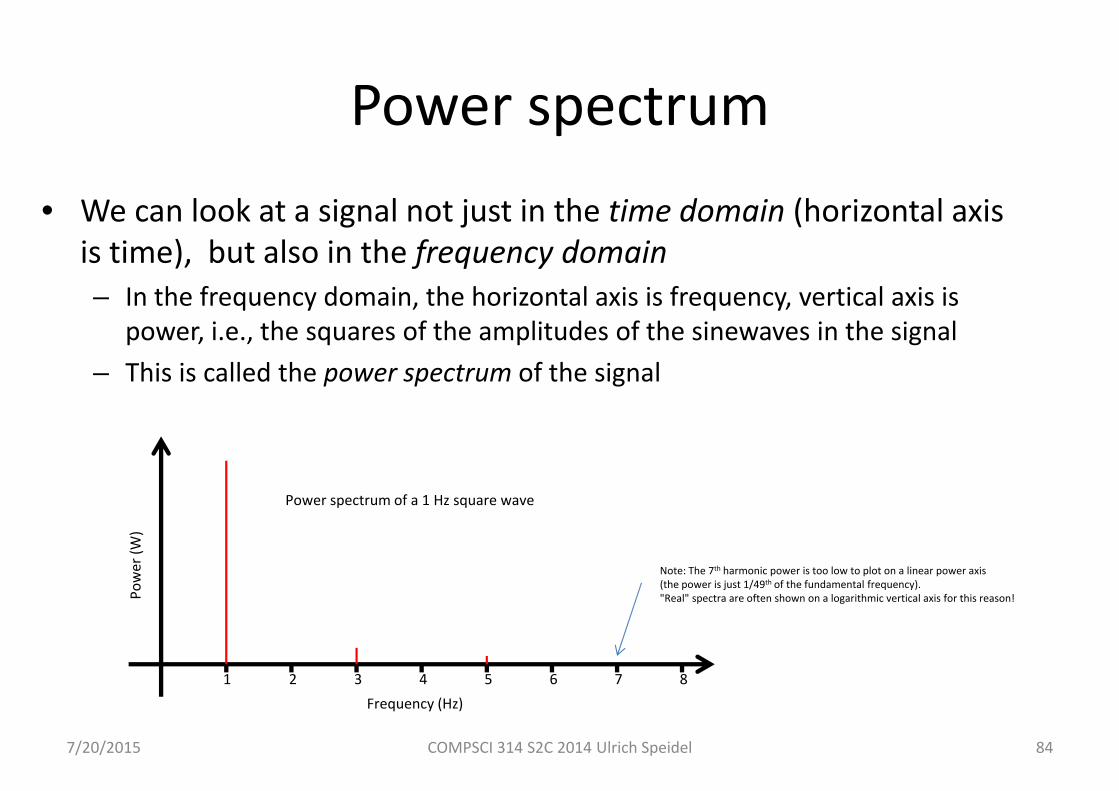
Power spectrum• We can look at a signal not just in the time domain (horizontal axis
is time), but also in the frequency domain– In the frequency domain, the horizontal axis is frequency, vertical axis is
power, i.e., the squares of the amplitudes of the sinewaves in the signal– This is called the power spectrum of the signal
7/20/2015 COMPSCI 314 S2C 2014 Ulrich Speidel 84
1 2 3 4 5 6 7 8Frequency (Hz)
Power (W
)
Power spectrum of a 1 Hz square wave
Note: The 7th harmonic power is too low to plot on a linear power axis (the power is just 1/49th of the fundamental frequency)."Real" spectra are often shown on a logarithmic vertical axis for this reason!

Bandwidth and power spectrum of a signal
• The difference between the highest and lowest (significant) frequency component in a signal’s power spectrum represents the signal’s bandwidth
• In communications, the term bandwidth is used to describe both the width of the frequency band available for a signal and the width of the signal’s actual power spectrum. Which bandwidth we mean should generally be apparent from the context.
7/20/2015 COMPSCI 314 S2C 2014 Ulrich Speidel 85
Week 2
• Lecture 4: Modulation
• Lecture 5: Constellation diagrams
• Lecture 6: Noise and the Shannon‐Hartley capacity theorem
7/20/2015 COMPSCI 314 S2C 2014 Ulrich Speidel 86
Lecture 4
• Modulation
• Amplitude modulation
• Frequency modulation
• Phase modulation
7/20/2015 COMPSCI 314 S2C 2014 Ulrich Speidel 87

7/20/2015 COMPSCI 314 S2C 2014 Ulrich Speidel 88
Modulation
• Modulation is the term for shaping an analog signal waveform in order to transmit analog or digital information
• Modulation is used in radio communication and also for modem communication
• The basic three types of modulation are amplitude modulation, frequency modulation, and phase modulation

7/20/2015 COMPSCI 314 S2C 2014 Ulrich Speidel 89
Amplitude Modulation (AM)
• Vary the amplitude of a carrier signal depending on the amplitude of the modulating signal that carries the information to be transmitted
• Crude example: for a binary (on or off) modulating signal, turn carrier on or off (Morse code on radio works that way)
• Can vary all or just part of the amplitude of the carrier• Called ASK (amplitude shift keying) in the discrete case (discrete case means that we vary in steps)

7/20/2015 COMPSCI 314 S2C 2014 Ulrich Speidel 90
AM in the time domain
Modulation of a 64 Hz sine wave with a pure sine wave of a Hz
7/20/2015 COMPSCI 314 S2C 2014 Ulrich Speidel 91
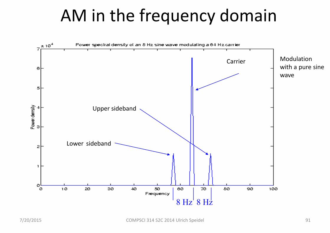
AM in the frequency domain
Carrier
Upper sideband
Lower sideband
8 Hz 8 Hz
Modulationwith a pure sinewave
7/20/2015 COMPSCI 314 S2C 2014 Ulrich Speidel 92
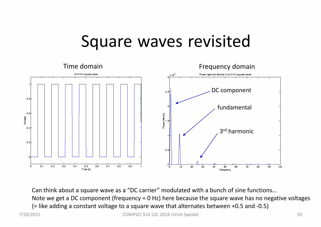
Square waves revisited
DC component
fundamental
3rd harmonic
Can think about a square wave as a “DC carrier” modulated with a bunch of sine functions…Note we get a DC component (frequency = 0 Hz) here because the square wave has no negative voltages(= like adding a constant voltage to a square wave that alternates between +0.5 and ‐0.5)
Time domain Frequency domain

7/20/2015 COMPSCI 314 S2C 2014 Ulrich Speidel 93
AM with a square wave in the time domain (Amplitude Shift Keying)
7/20/2015 COMPSCI 314 S2C 2014 Ulrich Speidel 94
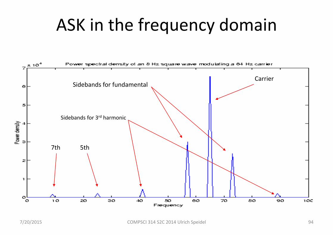
ASK in the frequency domain
CarrierSidebands for fundamental
Sidebands for 3rd harmonic
5th 7th
7/20/2015 COMPSCI 314 S2C 2014 Ulrich Speidel 95
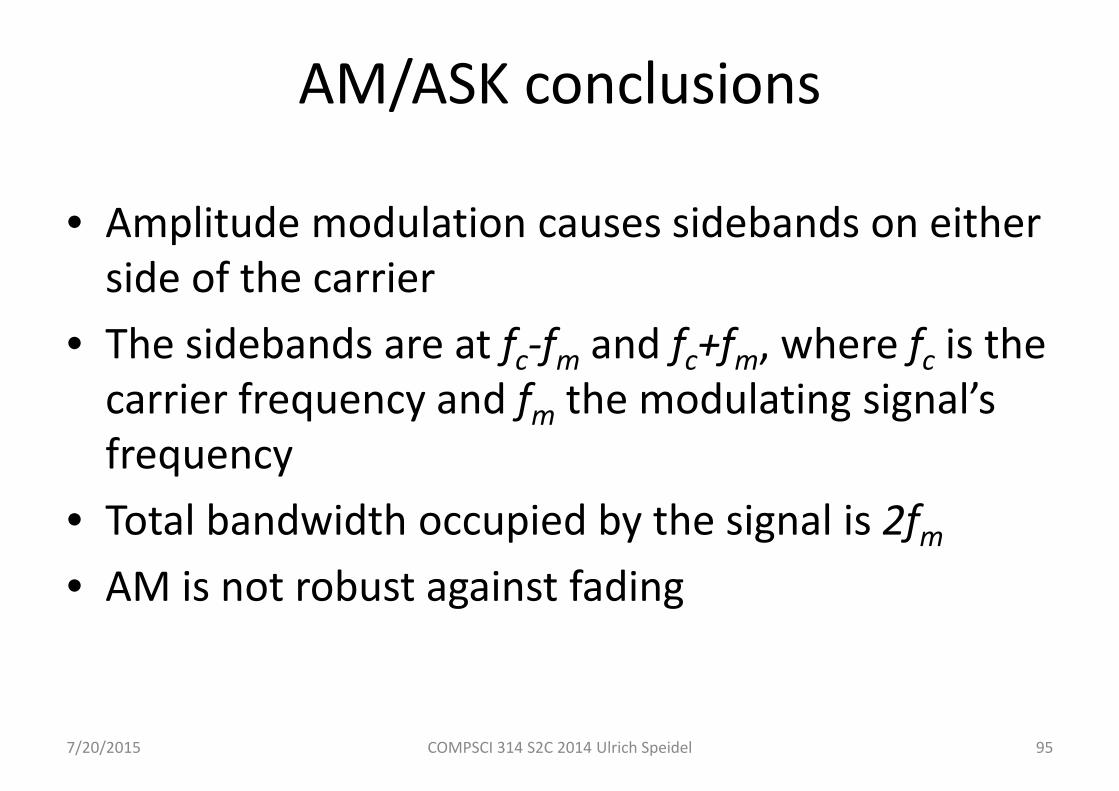
AM/ASK conclusions
• Amplitude modulation causes sidebands on either side of the carrier
• The sidebands are at fc‐fm and fc+fm, where fc is the carrier frequency and fm the modulating signal’s frequency
• Total bandwidth occupied by the signal is 2fm• AM is not robust against fading

7/20/2015 COMPSCI 314 S2C 2014 Ulrich Speidel 96
Frequency modulation (FM)
• Vary the frequency of a sinusoidal carrier signal with the amplitude of the modulating signal
• More robust modulation scheme if used on its own – we always transmit the carrier at full power
• Usually takes more bandwidth than AM• Called FSK (frequency shift keying) in the discrete case
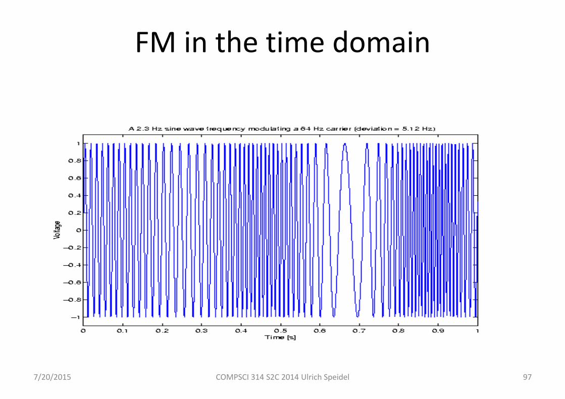
7/20/2015 COMPSCI 314 S2C 2014 Ulrich Speidel 97
FM in the time domain

7/20/2015 COMPSCI 314 S2C 2014 Ulrich Speidel 98
FM in the frequency domain
FM tends to have lots of sidebands
7/20/2015 COMPSCI 314 S2C 2014 Ulrich Speidel 99
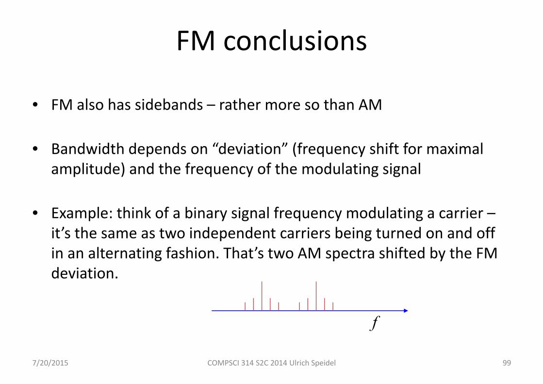
FM conclusions
• FM also has sidebands – rather more so than AM
• Bandwidth depends on “deviation” (frequency shift for maximal amplitude) and the frequency of the modulating signal
• Example: think of a binary signal frequency modulating a carrier –it’s the same as two independent carriers being turned on and off in an alternating fashion. That’s two AM spectra shifted by the FM deviation.
f

7/20/2015 COMPSCI 314 S2C 2014 Ulrich Speidel 100
FSK in the frequency domain…
Told you so!

7/20/2015 COMPSCI 314 S2C 2014 Ulrich Speidel 101
Phase modulation (PM)
• Vary phase of carrier signal to follow the amplitude of the modulating signal
• Looks very similar to FM in many respects. In the analog case, FM receivers can generally be used to receive PM transmissions and vice versa
• Called PSK (phase shift keying) in the discrete case
7/20/2015 COMPSCI 314 S2C 2014 Ulrich Speidel 102
PM conclusions
• Sidebands depend on amount of phase shift (think of the “sharpness” of the phase jump in a digital transmission) and the frequency of the modulating signal
• In the PSK case, we get discrete sidebands
7/20/2015 COMPSCI 314 S2C 2014 Ulrich Speidel 103
Combining AM and PM
• Can modulate both amplitude and phase of a carrier signal by generating a linear combination of a sine and a cosine wave of the carrier frequency:
s(t)=I sin(2πfct) + Q cos(2πfct)
• By choosing I and Q, we have states in a two‐dimensional state space. The frequency (carrier) does not change with time.
• A set of such states is called a constellation. A constellation can be depicted graphically as a constellation diagram.
Lecture 5
• Constellation diagrams
• BPSK
• QPSK
• 16‐QAM
7/20/2015 COMPSCI 314 S2C 2014 Ulrich Speidel 104

7/20/2015 COMPSCI 314 S2C 2014 Ulrich Speidel 105
Constellation diagram:Standard binary PSK
Q
I
The distance between the twostates determines the robustness of the scheme (but also the power that is needed for transmission!)
• Two states with same amplitude (distance from origin)
• 180 degrees apart
7/20/2015 COMPSCI 314 S2C 2014 Ulrich Speidel 106
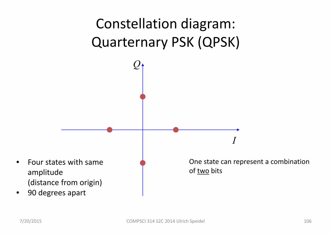
Constellation diagram:Quarternary PSK (QPSK)
Q
I
One state can represent a combination of two bits
• Four states with same amplitude (distance from origin)
• 90 degrees apart
7/20/2015 COMPSCI 314 S2C 2014 Ulrich Speidel 107
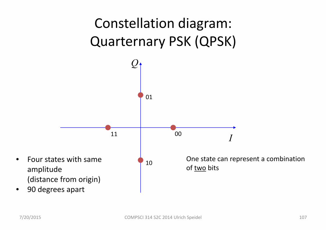
Constellation diagram:Quarternary PSK (QPSK)
Q
I
One state can represent a combination of two bits
• Four states with same amplitude (distance from origin)
• 90 degrees apart
00
01
11
10
7/20/2015 COMPSCI 314 S2C 2014 Ulrich Speidel 108
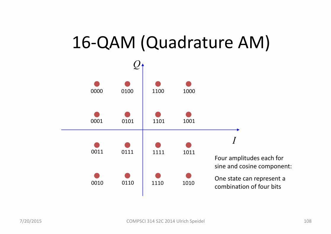
16‐QAM (Quadrature AM) Q
IFour amplitudes each forsine and cosine component:
One state can represent a combination of four bits
0000
0001
0011
0010
0100
0101
0111
0110
1100
1101
1111
1110
1000
1001
1011
1010
Gray coding
• Look at the neighbouring constellation points in the 16‐QAM scheme.
• They all differ be exactly one bit. This is known as a Gray code.
• Using a Gray code means that if we end up decoding a neighbouring constellation point, we only get one incorrect bit.
7/20/2015 COMPSCI 314 S2C 2014 Ulrich Speidel 109

Things worth knowing• 16QAM is not the limit – there are schemes with more constellation points (up to 256x256
constellation points in 65536‐QAM)
• Used in DSL/ADSL (where multiple high‐frequency tones – much like the keys on a piano ‐are each QAM modulated in parallel)
• Also used in radio communication and in optical communication
• The number of symbols (constellation points) we transmit per second is known as the Baud rate. It is not normally the same as the bit rate, except when there are only two constellation points (e.g., BPSK).
• In 16QAM, there are four bits per symbol, so we get a bit rate that is four times the Baud rate.
7/20/2015 COMPSCI 314 S2C 2014 Ulrich Speidel 110

7/20/2015 COMPSCI 314 S2C 2014 Ulrich Speidel 111
Constellation diagram summary
• Can modulate an audio signal or radio signal in both phase and amplitude
• Can do this in a number of different constellations (see signal constellation diagrams)
• Distance between adjacent constellation points determines robustness
Lecture 6
• Noise
• Noise in constellation diagrams
• The Shannon‐Hartley capacity theorem
7/20/2015 COMPSCI 314 S2C 2014 Ulrich Speidel 112
7/20/2015 COMPSCI 314 S2C 2014 Ulrich Speidel 113
Signal degradation
• A signal sent by a transmitter does not normally arrive at the receiver without having been degraded in some way
• A signal may lose amplitude through spreading
• A signal may lose amplitude through attenuation in the medium it propagates in (e.g., light in a fibre is absorbed by the glass)
• A signal may get distorted because some of its constituting frequency components (‐>Fourier analysis) get attenuated by different amounts or propagate at different speeds or on different paths. This can sometimes be reversed by appropriate filtering.
• A signal may get corrupted by additive noise on the channel it propagates through
7/20/2015 COMPSCI 314 S2C 2014 Ulrich Speidel 114
Noise
• Noise is a random signal that is added to a signal to be transmitted by the medium/channel that the signal is traveling through
• The power spectrum of noise may be flat or have some shape
• Noise with a flat power spectrum is called “white noise”. It often has a thermal origin (electrons bouncing around electronic components).
• In Fourier analysis, we can think of white noise as having components for all frequencies, such that the phases are random. Its amplitude distribution is often assumed to be Gaussian (i.e., the probability of a component having a certain amplitude A decreases as A increases).
• Noise is present in all practical communication channels. We can measure noise power across a given bandwidth in watts per hertz (W/Hz).

7/20/2015 COMPSCI 314 S2C 2014 Ulrich Speidel 115
The effect of signal degradation I
Q
State transmitted
State received
Decision boundary
(no error)
7/20/2015 COMPSCI 314 S2C 2014 Ulrich Speidel 116
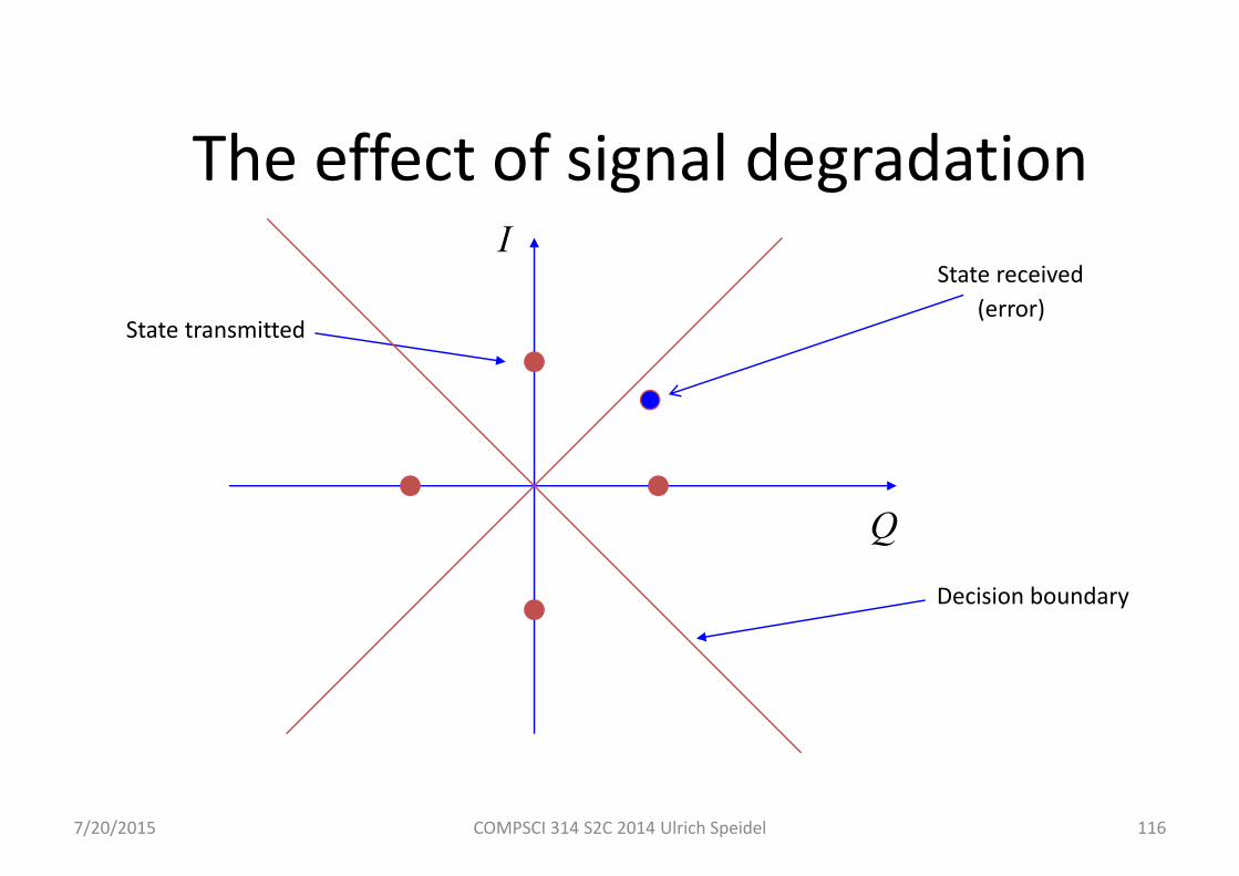
The effect of signal degradation I
Q
State transmitted
State received
Decision boundary
(error)
7/20/2015 COMPSCI 314 S2C 2014 Ulrich Speidel 117
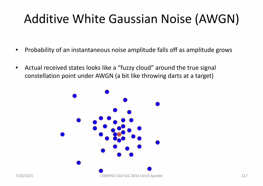
Additive White Gaussian Noise (AWGN)
• Probability of an instantaneous noise amplitude falls off as amplitude grows
• Actual received states looks like a “fuzzy cloud” around the true signal constellation point under AWGN (a bit like throwing darts at a target)

7/20/2015 COMPSCI 314 S2C 2014 Ulrich Speidel 118
Actual effects of noise
• How much effect noise has depends on two factors:– The noise level (average noise power) = “diameter of the cloud”– The signal level = distance to the nearest neighbour in the constellation
• Signal‐to‐noise ratio (SNR) defines how close the detected signal constellation points come to the sector(s) of constellation points other than that of the transmitted signal
• The SNR is the ratio between the size of the non‐overlapping circular area around each constellation point and the area occupied by the “noise cloud” (determined by the noise power)
• Detecting an incorrect constellation point constitutes a symbol error
7/20/2015 COMPSCI 314 S2C 2014 Ulrich Speidel 119
Actual effects of noise
• Depending on the number of states in the constellation, a wrongly detected state may lead to one or more bit errors
• Can use Gray code to minimize number of bit errors –choose bit assignment to constellation points such that adjacent states differ in as few bits as possible
• Can use signal‐to‐noise ratio (SNR) to estimate bit error rate: the higher the SNR, the fewer bit errors you get
Observations (I)• The area in which we can accommodate our constellation points is determined by the
square of the maximum sine and cosine amplitude we can transmit with (area of circle around the origin going through the furthest constellation point away from the origin).
• This area corresponds to a square of a voltage, so represents a power. Divide this power by the number of constellation points (symbols) and we get the power per symbol.
• If the noise power exceeds the power per symbol, we’ll routinely get symbol errors. So, if we have a choice of constellation, the size of the noise cloud (noise power) that the channel adds to the constellation points determines the maximum number of constellation points we can accommodate within a given radius (amplitude) around the origin.
7/20/2015 COMPSCI 314 S2C 2014 Ulrich Speidel 120

Observations (II)• Let S be the signal power and N the noise power in our given band. Then S/N is
the signal‐to‐noise ratio (SNR) and the number of feasible constellation points is S/N.
• The number of bits per symbol is thus log2(S/N).
• All this happens within a bandwidth that we may assume supports our chosen symbol rate (i.e., we spend sufficient time in the vicinity of each constellation point in order for it to be detected => Fourier analysis).
• If we had n times the bandwidth, we could replicate the scheme and gain n times the symbol rate. Conclusion: symbol rate converts to bit rate proportional to bandwidth!
7/20/2015 COMPSCI 314 S2C 2014 Ulrich Speidel 121
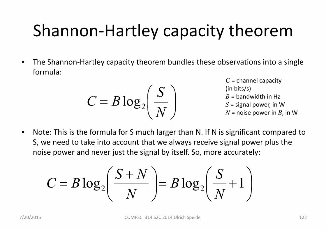
Shannon‐Hartley capacity theorem• The Shannon‐Hartley capacity theorem bundles these observations into a single
formula:
• Note: This is the formula for S much larger than N. If N is significant compared to S, we need to take into account that we always receive signal power plus the noise power and never just the signal by itself. So, more accurately:
7/20/2015 COMPSCI 314 S2C 2014 Ulrich Speidel 122
NSBC 2log
1loglog 22 NSB
NNSBC
C = channel capacity(in bits/s)B = bandwidth in HzS = signal power, in WN = noise power in B, in W
Shannon‐Hartley interpreted• The more bandwidth we have, the higher the rate at which we can communicate.
• The more transmit power we use, the higher the possible bit rate.
• The lower the noise, the higher the bit rate we’ll be able to sustain in a given bandwidth with a given transmit power.
• Note: S is actually the signal power available at the receiver (i.e., whatever is left over from the power with which the signal was transmitted). This can be many orders of magnitude less than the actual transmit power, but it scales with the transmit power!
7/20/2015 COMPSCI 314 S2C 2014 Ulrich Speidel 123
Shannon‐Hartley notes• The Shannon‐Hartley capacity theorem places a fundamental limit on the bit rate
we can theoretically achieve in a given bandwidth under given channel conditions.
• It means we can’t simply “transmit faster” without either spilling over into adjacent frequency bands and/or introducing an increasing number of bit errors.
• In practice, it can be quite difficult to achieve the bit rate that the Shannon‐Hartley capacity theorem promises. This is a very active area of research in information theory, and a pressing one, too!
7/20/2015 COMPSCI 314 S2C 2014 Ulrich Speidel 124

Week 3
• Lecture 7: Symbol errors and error detection/correction
• Lecture 8: Hamming codes, LDPC codes, network coding
• Lecture 9: Clocking and synchronisation
7/20/2015 COMPSCI 314 S2C 2014 Ulrich Speidel 125
Lecture 7
• Symbol errors
• Parity error detection / correction
• Cyclic redundancy checks (Checksums)
7/20/2015 COMPSCI 314 S2C 2014 Ulrich Speidel 126
Symbol errors revisited
7/20/2015 COMPSCI 314 S2C 2014 Ulrich Speidel 127
I
Q
State transmitted
State received
Decision boundary
(error)
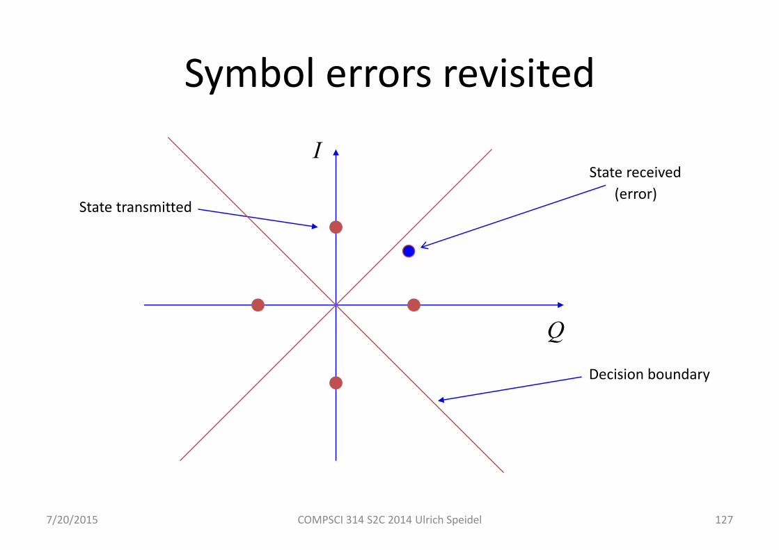
Symbol errors revisited
• A symbol error happens when noise or distortion added on the channel cause the received signal to fall outside the intended constellation state’s discriminator region
• As each symbol maps to one or more bits, this means that one or more bits will be in error
• When symbol / bit errors happen, there are a number of ways in which this may be dealt with
7/20/2015 COMPSCI 314 S2C 2014 Ulrich Speidel 128
Error handling strategies
• Do nothing: – In this case, the receiver will use / output incorrect data– This may be acceptable under certain circumstances (e.g., real‐time
streaming audio)
• Error detection:– Receiver may substitute incorrect data by defaults or may re‐request correct
version from transmitter (automatic repeat request – ARQ)– Requires encoding to enable errors to be detected
• Error correction:– Use remaining data to reconstruct the original transmission– Requires encoding to enable errors to be detected and corrected
7/20/2015 COMPSCI 314 S2C 2014 Ulrich Speidel 129

Error detection
• Error detection is used in two contexts– If we are able to substitute the data (e.g., in an image, replace a pixel value
by an interpolation of neighbouring pixel values)– If we are able to re‐request the correct data from the transmitter. This
requires a bi‐directional channel (e.g., duplex, semi‐duplex, many‐to‐many, or one‐to‐one shared). This is called ARQ (Automatic Repeat Request)
• Error detection requires additional information (redundancy) to be transmitted along with the data. Examples:– Parity bits– Checksums (CRC, hashes)
7/20/2015 COMPSCI 314 S2C 2014 Ulrich Speidel 130
Error correction
• Error correction may be used when:– We are not able to substitute or re‐request data, or– when re‐requesting data is not feasible due to the turnaround time, or not
economical
• Error correction also requires the transmission of redundant information – as a rule more than for mere error detection. Examples:– Hamming codes– Reed‐Solomon codes (as used on CDs)– advanced codes such as convolutional codes, turbo codes, Low Density Parity
Check codes (LDPC codes), and others
7/20/2015 COMPSCI 314 S2C 2014 Ulrich Speidel 131
Brute force approach to error correction
7/20/2015 COMPSCI 314 S2C 2014 Ulrich Speidel 132
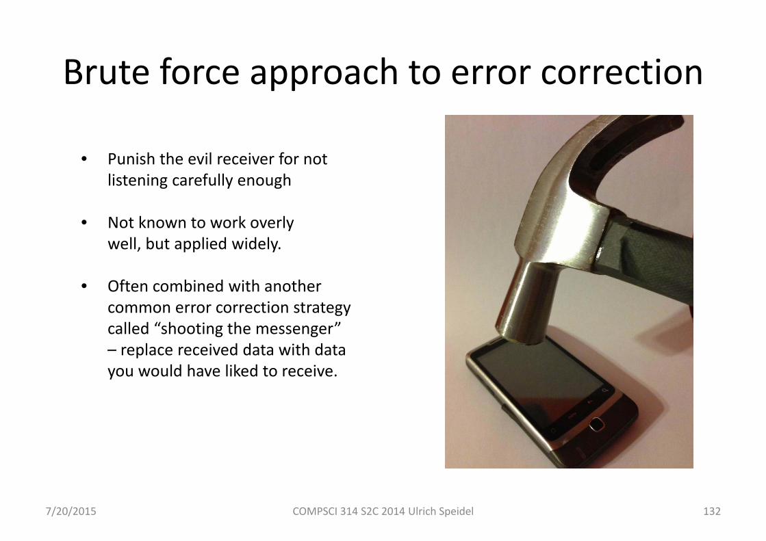
• Punish the evil receiver for not listening carefully enough
• Not known to work overlywell, but applied widely.
• Often combined with another common error correction strategy called “shooting the messenger” – replace received data with data you would have liked to receive.
7/20/2015 COMPSCI 314 S2C 2014 Ulrich Speidel 133
Parity bits• The data we wish to transmit is called the payload data
• Add an additional bit (the parity bit) to each byte of payload data
• Two types of parity (we may choose either):– Even parity: the parity bit is set such that the total number of 1‐bits including the parity bit itself is even
– Odd parity: the parity bit is set such that the total number of 1‐bits including the parity bit itself is odd
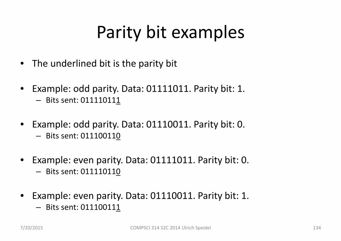
Parity bit examples• The underlined bit is the parity bit
• Example: odd parity. Data: 01111011. Parity bit: 1. – Bits sent: 011110111
• Example: odd parity. Data: 01110011. Parity bit: 0. – Bits sent: 011100110
• Example: even parity. Data: 01111011. Parity bit: 0. – Bits sent: 011110110
• Example: even parity. Data: 01110011. Parity bit: 1. – Bits sent: 011100111
7/20/2015 COMPSCI 314 S2C 2014 Ulrich Speidel 134
Parity checks
• Assume a single bit inversion error (bit in italics) in the third bit odd parity example from the previous slide:– That is, 011110111 turns into 010110111
• The receiver tests of odd parity but only finds six 1 bits (including the parity bit) ‐> error detected– Can’t determine which bit(s) are inverted?– What happens if two or more bits are in error?– What happens if only the parity bit is inverted? What is the probability of this happening?
7/20/2015 COMPSCI 314 S2C 2014 Ulrich Speidel 135

7/20/2015 COMPSCI 314 S2C 2014 Ulrich Speidel 136
Checksums and digests
• Checksums in data communication are often implemented as CRCs (cyclic redundancy checksums)
• Digests are like checksums, except that we presume that we want to guard the data against “intelligent interference” (i.e., when someone is deliberately trying to modify our data in transit). The algorithms for digests are generally more complex from a computational point of view
• Think of both checksums and digests as hash functions – except that we make no attempt to resolve any collisions of hash values
7/20/2015 COMPSCI 314 S2C 2014 Ulrich Speidel 137
CRC Checksums
• Based on modulo‐2 division of polynomials
• In practice, either 16 bit or 32 bit CRCs are used in many data communication applications, e.g., Ethernet frame protection
• Need to understand polynomial division and modulo‐2 arithmetic for this
7/20/2015 COMPSCI 314 S2C 2014 Ulrich Speidel 138
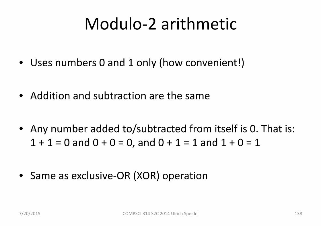
Modulo‐2 arithmetic
• Uses numbers 0 and 1 only (how convenient!)
• Addition and subtraction are the same
• Any number added to/subtracted from itself is 0. That is: 1 + 1 = 0 and 0 + 0 = 0, and 0 + 1 = 1 and 1 + 0 = 1
• Same as exclusive‐OR (XOR) operation

7/20/2015 COMPSCI 314 S2C 2014 Ulrich Speidel 139
Polynomial division in modulo‐2
• Coefficients of polynomials under modulo‐2 …. are just bits, one bit per coefficient!
• Look at payload as a polynomial ‐ its bits are the coefficients
• E.g., 10011011 is equivalent to:
x7+x4+x3+x+1 = 1 x7+ 0 x6 + 0 x5 + 1 x4 + 1 x3+ 0 x2+ 1 x1 + 1 x0
• Division works like long division of decimal numbers – but the rules of modulo 2 make it a little easier
• Example: Divide 100110110000 by 11001 modulo‐2
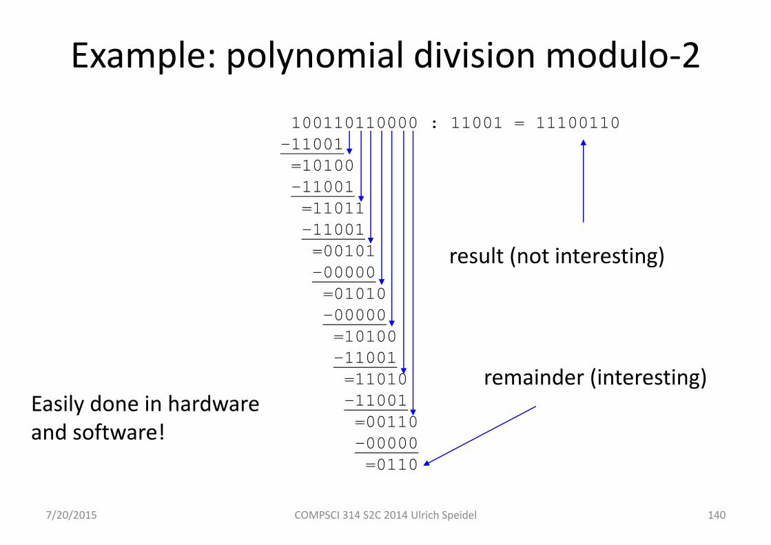
7/20/2015 COMPSCI 314 S2C 2014 Ulrich Speidel 140
Example: polynomial division modulo‐2100110110000 : 11001 = 11100110-11001=10100-11001=11011-11001=00101-00000=01010-00000=10100-11001=11010-11001=00110-00000=0110
remainder (interesting)
result (not interesting)
Easily done in hardwareand software!
7/20/2015 COMPSCI 314 S2C 2014 Ulrich Speidel 141
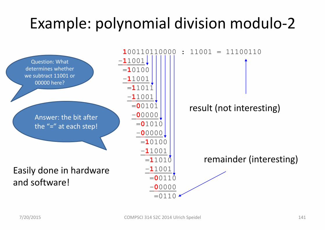
Example: polynomial division modulo‐2100110110000 : 11001 = 11100110-11001=10100-11001=11011-11001=00101-00000=01010-00000=10100-11001=11010-11001=00110-00000=0110
remainder (interesting)
result (not interesting)
Easily done in hardwareand software!
Question: What determines whether we subtract 11001 or
00000 here?
Answer: the bit after the “=” at each step!
7/20/2015 COMPSCI 314 S2C 2014 Ulrich Speidel 142
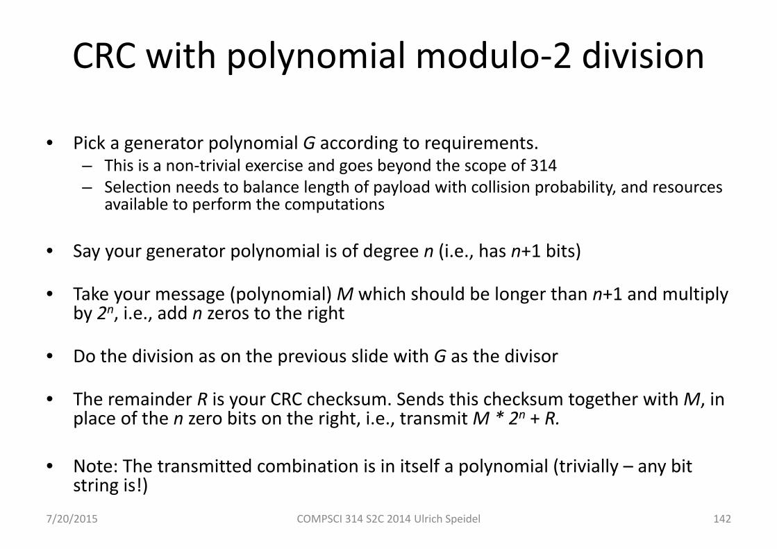
CRC with polynomial modulo‐2 division
• Pick a generator polynomial G according to requirements.– This is a non‐trivial exercise and goes beyond the scope of 314– Selection needs to balance length of payload with collision probability, and resources
available to perform the computations
• Say your generator polynomial is of degree n (i.e., has n+1 bits)
• Take your message (polynomial) M which should be longer than n+1 and multiply by 2n, i.e., add n zeros to the right
• Do the division as on the previous slide with G as the divisor
• The remainder R is your CRC checksum. Sends this checksum together with M, in place of the n zero bits on the right, i.e., transmit M * 2n + R.
• Note: The transmitted combination is in itself a polynomial (trivially – any bit string is!)
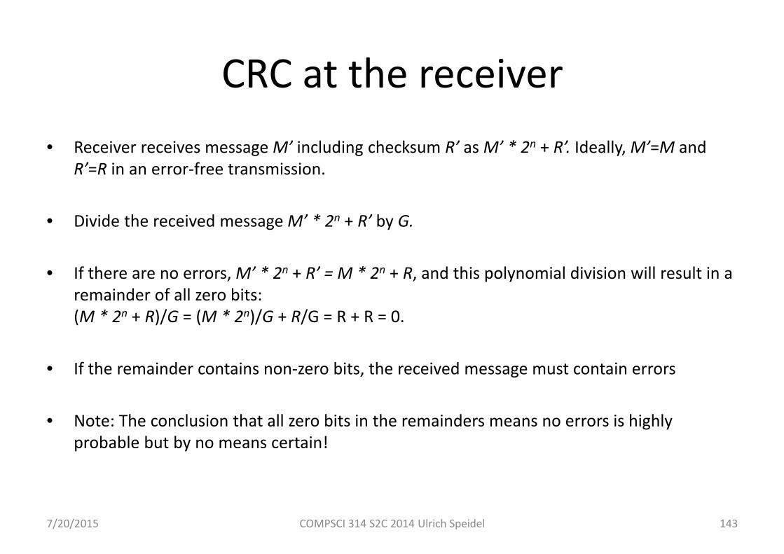
CRC at the receiver• Receiver receives message M’ including checksum R’ as M’ * 2n + R’. Ideally, M’=M and
R’=R in an error‐free transmission.
• Divide the received message M’ * 2n + R’ by G.
• If there are no errors, M’ * 2n + R’ = M * 2n + R, and this polynomial division will result in a remainder of all zero bits: (M * 2n + R)/G = (M * 2n)/G + R/G = R + R = 0.
• If the remainder contains non‐zero bits, the received message must contain errors
• Note: The conclusion that all zero bits in the remainders means no errors is highly probable but by no means certain!
7/20/2015 COMPSCI 314 S2C 2014 Ulrich Speidel 143

100110110000 : 11001 = 11100110-11001=10100-11001=11011-11001=00101-00000=01010-00000=10100-11001=11010-11001=00110-00000=0110
7/20/2015 COMPSCI 314 S2C 2014 Ulrich Speidel 144
Example: Computation of CRC
remainder (CRC)
result (not that interesting)
last n=4 bits (blue) reserved for CRC
G
Transmitter side
Bits sent:
100110110110
M * 2n
M * 2n + R
7/20/2015 COMPSCI 314 S2C 2014 Ulrich Speidel 145
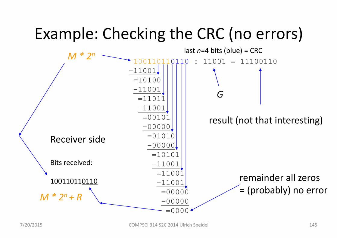
100110110110 : 11001 = 11100110-11001=10100-11001=11011-11001=00101-00000=01010-00000=10101-11001=11001-11001=00000-00000=0000
Example: Checking the CRC (no errors)
remainder all zeros= (probably) no error
result (not that interesting)
last n=4 bits (blue) = CRC
G
Receiver side
Bits received:
100110110110
M * 2n
M * 2n + R
7/20/2015 COMPSCI 314 S2C 2014 Ulrich Speidel 146
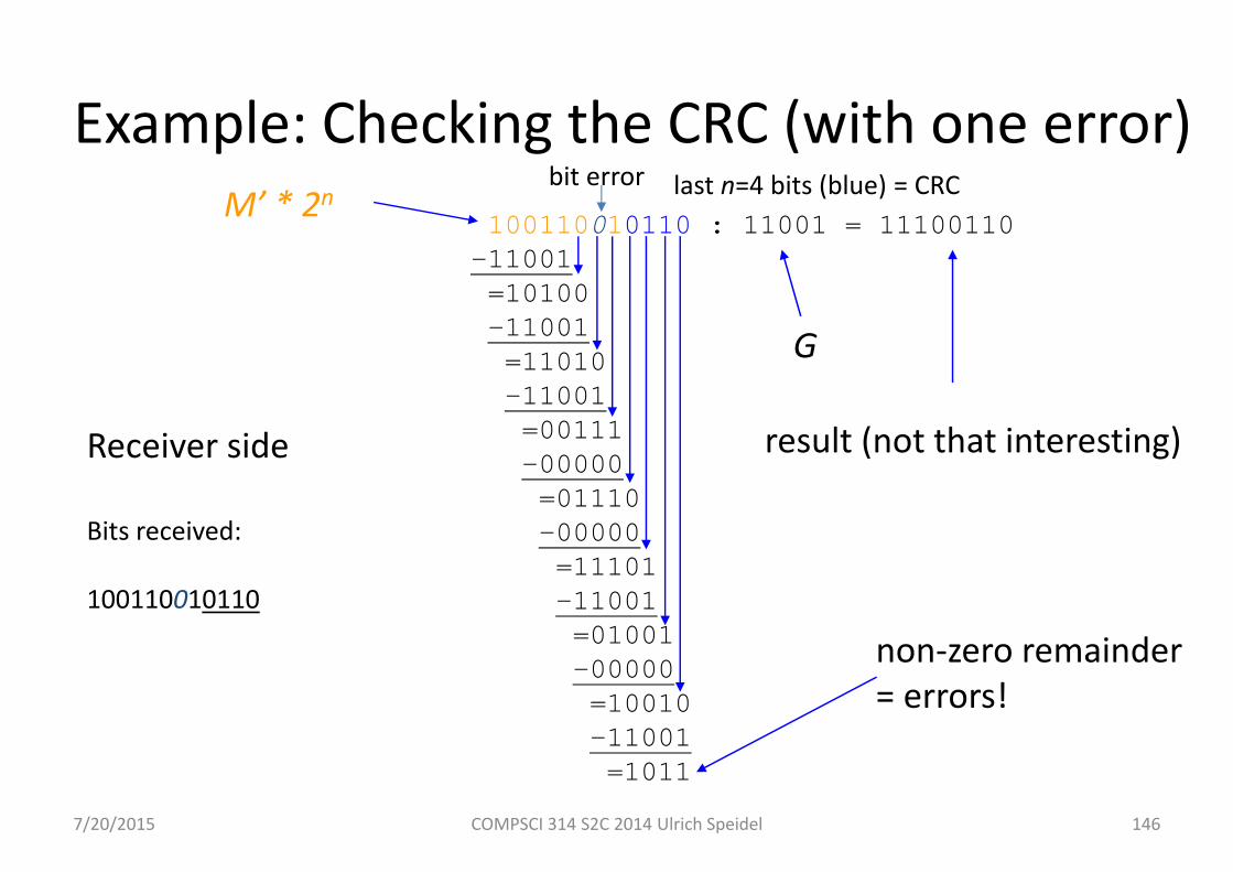
100110010110 : 11001 = 11100110-11001=10100-11001=11010-11001=00111-00000=01110-00000=11101-11001=01001-00000=10010-11001=1011
Example: Checking the CRC (with one error)
non‐zero remainder= errors!
result (not that interesting)
last n=4 bits (blue) = CRC
G
Receiver side
Bits received:
100110010110
M’ * 2nbit error

Lecture 8
• Error correction with Hamming codes
• LDPC codes
• Network coding
7/20/2015 COMPSCI 314 S2C 2014 Ulrich Speidel 147
7/20/2015 COMPSCI 314 S2C 2014 Ulrich Speidel 148
Error correction with Hamming codes
• Error detection is best used when the receiver has a way of coping with the data loss (e.g., the ability to ask the transmitter for a fresh copy of a packet)
• This is often either not possible or not practical, e.g., because of high latency in cases where data is needed immediately (streaming audio / video or VoIP)
• If we cannot re‐request data, we may need to attempt error correction based on what we have received
• Hamming Codes are perhaps the simplest example for error correction
• In Hamming codes, we protect a bit string with several parity bits. The combination of parity bits that are in error lets us work out which bit is in error
7/20/2015 COMPSCI 314 S2C 2014 Ulrich Speidel 149
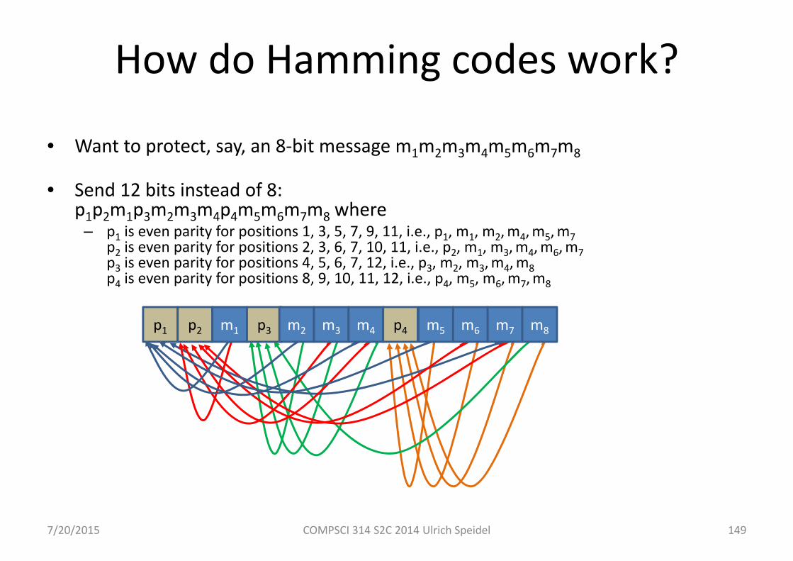
How do Hamming codes work?
• Want to protect, say, an 8‐bit message m1m2m3m4m5m6m7m8
• Send 12 bits instead of 8:p1p2m1p3m2m3m4p4m5m6m7m8 where
– p1 is even parity for positions 1, 3, 5, 7, 9, 11, i.e., p1, m1, m2,m4,m5,m7p2 is even parity for positions 2, 3, 6, 7, 10, 11, i.e., p2, m1, m3,m4,m6,m7p3 is even parity for positions 4, 5, 6, 7, 12, i.e., p3, m2, m3,m4,m8p4 is even parity for positions 8, 9, 10, 11, 12, i.e., p4, m5, m6,m7,m8
p1 p2 m1 p3 m2 m3 m4 p4 m5 m6 m7 m8
7/20/2015 COMPSCI 314 S2C 2014 Ulrich Speidel 150
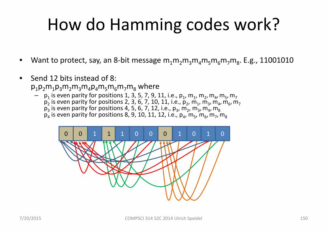
How do Hamming codes work?
• Want to protect, say, an 8‐bit message m1m2m3m4m5m6m7m8. E.g., 11001010
• Send 12 bits instead of 8:p1p2m1p3m2m3m4p4m5m6m7m8 where
– p1 is even parity for positions 1, 3, 5, 7, 9, 11, i.e., p1, m1, m2,m4,m5,m7p2 is even parity for positions 2, 3, 6, 7, 10, 11, i.e., p2, m1, m3,m4,m6,m7p3 is even parity for positions 4, 5, 6, 7, 12, i.e., p3, m2, m3,m4,m8p4 is even parity for positions 8, 9, 10, 11, 12, i.e., p4, m5, m6,m7,m8
0 0 1 1 1 0 0 0 1 0 1 0
7/20/2015 COMPSCI 314 S2C 2014 Ulrich Speidel 151
How do Hamming codes work?
• Can now pinpoint where an error occurred: each data bit is protected by at least two parity bits, each parity bit only protects itself.
• Receiver re‐computes its own parity bits from data bits received and compares them with the parity bits received
• If parity bits are the same, then we have no error (probably)
• If only one parity bit does not compute to the same value at the receiver, the error is (probably) in the parity bit itself (note: for this type of Hamming code)
• If two parity bits fail to compute to the same value, then we can look at which data bits share both of these two parity bits. If they are shared by more than one bit, the remaining two (correct) parity bits will help us determine which data bit is in error.

7/20/2015 COMPSCI 314 S2C 2014 Ulrich Speidel 152
How do Hamming codes work?
• Want to protect, say, an 8‐bit message m1m2m3m4m5m6m7m8. E.g., 11001010
• Send 12 bits instead of 8:p1p2m1p3m2m3m4p4m5m6m7m8 where
– p1 is even parity for positions 1, 3, 5, 7, 9, 11, i.e., p1, m1, m2,m4,m5,m7p2 is even parity for positions 2, 3, 6, 7, 10, 11, i.e., p2, m1, m3,m4,m6,m7p3 is even parity for positions 4, 5, 6, 7, 12, i.e., p3, m2, m3,m4,m8p4 is even parity for positions 8, 9, 10, 11, 12, i.e., p4, m5, m6,m7,m8
0 0 1 1 1 0 0 0 1 1 1 0
• Example: Bit m6 in error• Parity bits p2 and p4
do not match at the receiver
• These bits are sharedby m6 and m7
• But: m7 is protectedby p1 as well
• p1 matches, so m7cannot be in error
• Conclusion: error is inm6. Correct to: m6=0
Limits of Hamming codes• The number of parity bits in a Hamming code determines how many errors we can correct
• E.g., the code with 8 data bits and 4 parity bits presented here can correct one error
• If there are additional errors, we may be able to detect them with Hamming code
• Example: Consider a situation in which parity bits p2, p3, and p4 don’t match
• As a general rule, the number of parity bits needed to correct a single data bit error is log2(number of data bits)+1
• Think of this conceptually as “number of bits needed to identify (address) the erroneous bit plus one parity bit to protect the parity bits”
7/20/2015 COMPSCI 314 S2C 2014 Ulrich Speidel 153
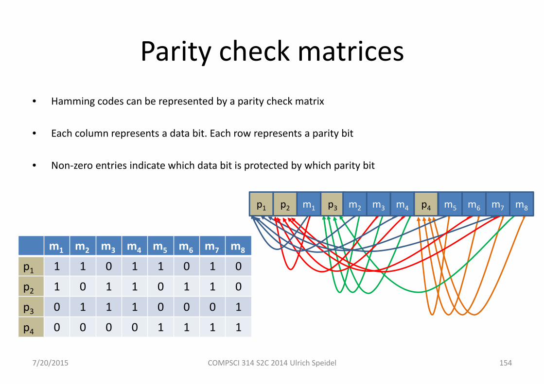
Parity check matrices• Hamming codes can be represented by a parity check matrix
• Each column represents a data bit. Each row represents a parity bit
• Non‐zero entries indicate which data bit is protected by which parity bit
7/20/2015 COMPSCI 314 S2C 2014 Ulrich Speidel 154
p1 p2 m1 p3 m2 m3 m4 p4 m5 m6 m7 m8
m1 m2 m3 m4 m5 m6 m7 m8
p1 1 1 0 1 1 0 1 0
p2 1 0 1 1 0 1 1 0
p3 0 1 1 1 0 0 0 1
p4 0 0 0 0 1 1 1 1
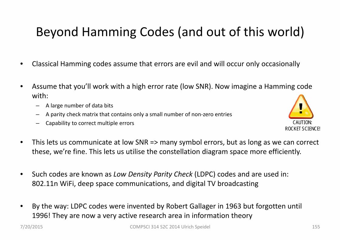
Beyond Hamming Codes (and out of this world)
• Classical Hamming codes assume that errors are evil and will occur only occasionally
• Assume that you’ll work with a high error rate (low SNR). Now imagine a Hamming code with:
– A large number of data bits– A parity check matrix that contains only a small number of non‐zero entries– Capability to correct multiple errors
• This lets us communicate at low SNR => many symbol errors, but as long as we can correct these, we’re fine. This lets us utilise the constellation diagram space more efficiently.
• Such codes are known as Low Density Parity Check (LDPC) codes and are used in:802.11n WiFi, deep space communications, and digital TV broadcasting
• By the way: LDPC codes were invented by Robert Gallager in 1963 but forgotten until 1996! They are now a very active research area in information theory
7/20/2015 COMPSCI 314 S2C 2014 Ulrich Speidel 155
CAUTION: ROCKET SCIENCE!
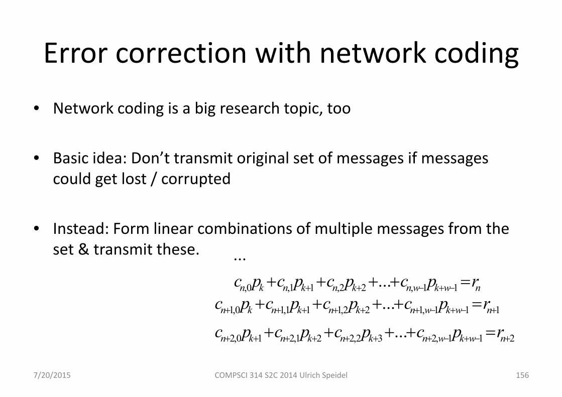
Error correction with network coding
• Network coding is a big research topic, too
• Basic idea: Don’t transmit original set of messages if messages could get lost / corrupted
• Instead: Form linear combinations of multiple messages from the set & transmit these.
7/20/2015 COMPSCI 314 S2C 2014 Ulrich Speidel 156
211,232,221,210,2
111,122,111,10,1
11,22,11,0,
.........
...
nwkwnknknkn
nwkwnknknkn
nwkwnknknkn
rpcpcpcpcrpcpcpcpc
rpcpcpcpc
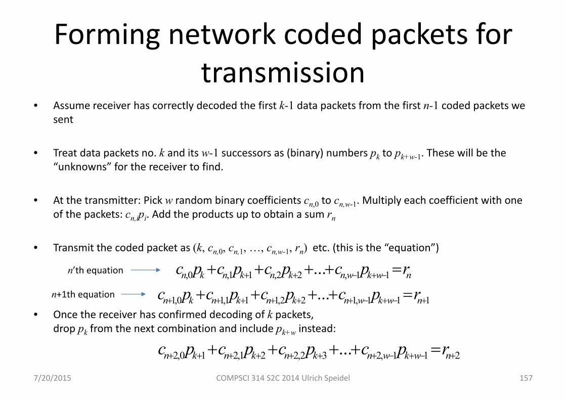
Forming network coded packets for transmission
• Assume receiver has correctly decoded the first k-1 data packets from the first n-1 coded packets we sent
• Treat data packets no. k and its w-1 successors as (binary) numbers pk to pk+w-1. These will be the “unknowns” for the receiver to find.
• At the transmitter: Pick w random binary coefficients cn,0 to cn,w-1. Multiply each coefficient with one of the packets: cn,ipi. Add the products up to obtain a sum rn
• Transmit the coded packet as (k, cn,0, cn,1, …, cn,w-1, rn) etc. (this is the “equation”)
• Once the receiver has confirmed decoding of k packets,drop pk from the next combination and include pk+w instead:
7/20/2015 COMPSCI 314 S2C 2014 Ulrich Speidel 157
111,122,111,10,1
11,22,11,0,
......
nwkwnknknkn
nwkwnknknkn
rpcpcpcpcrpcpcpcpc
211,232,221,210,2 ... nwkwnknknkn rpcpcpcpc
n’th equation
n+1th equation

Decoding network coded packets• Receiver recovers the original packets by solving the system of linear equations (you may remember
doing this in maths at some point or other)
• This is always possible once the receiver receives a sufficient number of equations containing the packet (“degrees of freedom”)
• Note: number of combinations (equations) matter, not the specific set of coefficients
• Transmitter keeps sending combinations of the same packets until it has confirmation of degrees of freedom at the receiver
• Lost combination packets don’t need to be retransmitted – the packet that follows can do the same job as a retransmission
• More info: See: Sundararajan, Shah, Médard, Mitzenmacher and Barros: “Network coding meets TCP”, http://arxiv.org/pdf/0809.5022.pdf
7/20/2015 COMPSCI 314 S2C 2014 Ulrich Speidel 158
Lecture 9
• Coding
• Clocking and synchronisation
• Bit stuffing and framing
7/20/2015 COMPSCI 314 S2C 2014 Ulrich Speidel 159

7/20/2015 COMPSCI 314 S2C 2014 Ulrich Speidel 160
Coding ‐ overview
• We encode information to facilitate its communication
• Encoding is not the same as encryption!
7/20/2015 COMPSCI 314 S2C 2014 Ulrich Speidel 161
Coding ‐ issues
• Adapt information to channel alphabet – not everything comes in bits
• Clocking and synchronisation – making sure the receiver knows what we’re at
• Error detection and correction (see previous lectures)
• Separating between messages
• Efficiency: Transmitting information with minimum unnecessary repetition
7/20/2015 COMPSCI 314 S2C 2014 Ulrich Speidel 162
Examples for codes
• Adapt information to channel alphabet: Morse code, ASCII
• Clocking and synchronization: Morse code, ASCII, Manchester, T‐codes, start/stop bits
• Error detection and correction (see previous lectures): Hamming codes, LDPC codes, parity, T‐codes
• Separating between messages: framing with bit stuffing (not actually a code in the classical sense), start/stop bits
• Efficiency: Transmitting information with minimum unnecessary repetition: Huffman codes, T‐codes

7/20/2015 COMPSCI 314 S2C 2014 Ulrich Speidel 163
Channel alphabet
• In electronic communications, we often have a channel alphabet with two letters which we can map to the bit values 0 and 1– E.g., high/low voltage, light in fibre on/off, BPSK constellation points
• Sometimes, a higher number of states are available and used– E.g., 4 in QPSK, 16 in 16QAM, 3 states (voltage positive/zero/negative), for example– Many of these can be mapped back to binary through bit combinations (e.g., 2 bits in
QPSK, 4 bits in 16QAM), but this is not always easy (e.g., for 3 states)
• The alphabet we might need to communicate in could be quite different: English, Chinese, German, Arabic
• Map higher order alphabets to binary using a code such as ASCII, Unicode, Morse
7/20/2015 COMPSCI 314 S2C 2014 Ulrich Speidel 164
Clocking
• Receiver needs to know when symbols (typically bits) on the channel begin and when they end
– Receiver ideally tries to sample the signal state in the middle of the bit period– If receiver knows the bit rate, the receiver’s clock will determine when to take the next sample
• But: Most real time bases (clocks) are a little bit inaccurate – transmitter and receiver clocks drift apart
– Typical quartz clock: a few seconds per day– Insertion errors: If the clock is too fast, we’ll sample “extra bits” by inadvertently sampling the
same bits twice – at 1 Mbps that’s several million bits a day!– Deletion errors: If the clock is too slow, we’ll skip bits instead– “Lattice fence effect”– A far more serious problem in the 1970’s where the predominant modem clocks were based on
resistors and capacitors – time constants could vary by as much as 20%
7/20/2015 COMPSCI 314 S2C 2014 Ulrich Speidel 165
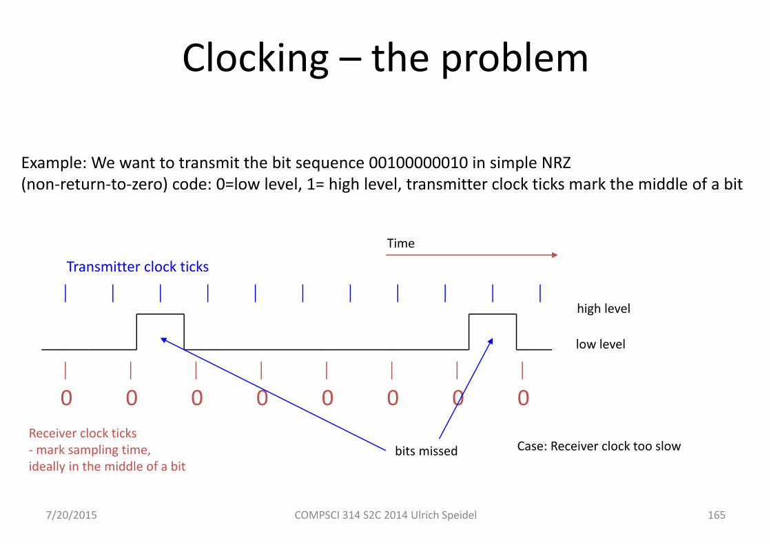
Clocking – the problem
Transmitter clock ticks
Example: We want to transmit the bit sequence 00100000010 in simple NRZ (non‐return‐to‐zero) code: 0=low level, 1= high level, transmitter clock ticks mark the middle of a bit
Time
low level
high level
Receiver clock ticks‐mark sampling time,ideally in the middle of a bit
bits missed
0 0 0 0 0 0 00
Case: Receiver clock too slow

7/20/2015 COMPSCI 314 S2C 2014 Ulrich Speidel 166
Clocking – the problem
Transmitter clock ticks
Example: We want to transmit the bit sequence 00100000010 in simple NRZ (non‐return‐to‐zero) code: 0=low level, 1= high level, transmitter clock ticks mark the middle of a bit
Time
low level
high level
Receiver clock ticks‐mark sampling time,ideally in the middle of a bit Bit received twice
0 1 1 0 0 0 00
Case: Receiver clock too fast
0 0 0 1 0
Additional 0 bit received
7/20/2015 COMPSCI 314 S2C 2014 Ulrich Speidel 167
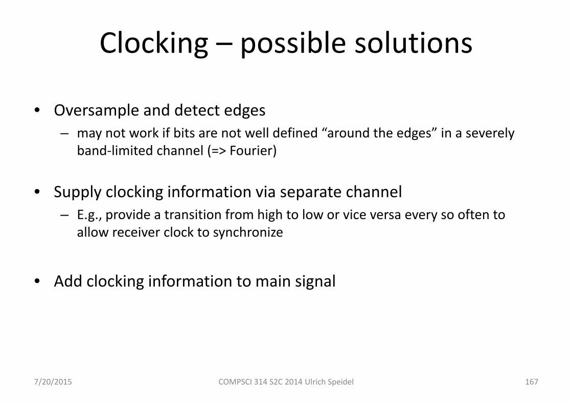
Clocking – possible solutions
• Oversample and detect edges– may not work if bits are not well defined “around the edges” in a severely
band‐limited channel (=> Fourier)
• Supply clocking information via separate channel– E.g., provide a transition from high to low or vice versa every so often to
allow receiver clock to synchronize
• Add clocking information to main signal
7/20/2015 COMPSCI 314 S2C 2014 Ulrich Speidel 168
Adding clocking information to a signal
• Methods in this category are generally known as “differential encoding” – baseband symbols are expressed as transitionsbetween channel states
• Example 1: NRZI (non‐return to zero inverted) with bit stuffing
• Example 2: Manchester coding
7/20/2015 COMPSCI 314 S2C 2014 Ulrich Speidel 169
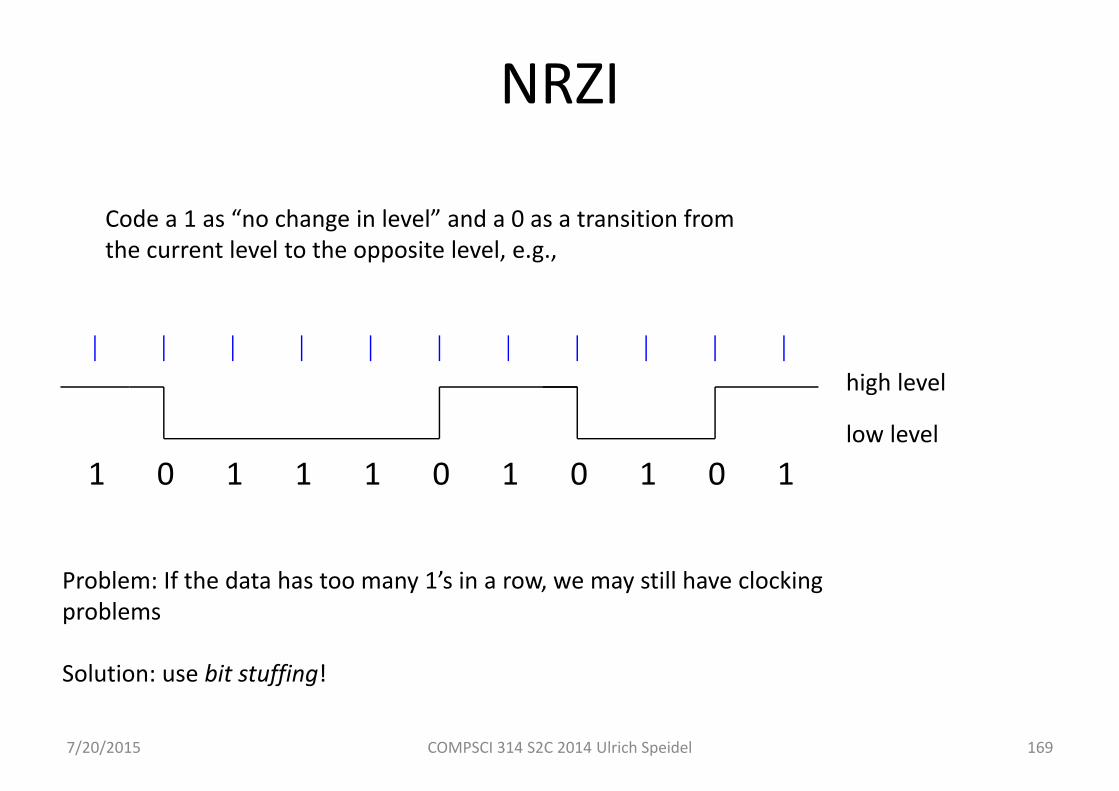
NRZI
Code a 1 as “no change in level” and a 0 as a transition fromthe current level to the opposite level, e.g.,
1 1 1 1 1 1 10 0 0 0
Problem: If the data has too many 1’s in a row, we may still have clocking problems
Solution: use bit stuffing!
low level
high level

7/20/2015 COMPSCI 314 S2C 2014 Ulrich Speidel 170
Bit stuffing
• Insert a 0 into the raw data after, e.g., every 5th consecutive 1 on the transmitter side
• This way, we have a guaranteed edge on which the receiver can synchronize itself
• On the receiver side, remove the 0‐bit that comes after every 5th consecutive 1
• Problems: Symbol rate varies with data, need to use queue buffers if signaling rate is to be constant. Receiver still needs own clock to predict next bit sampling time.
• Advantage: on average, few extra bits are inserted, bit stuffing is rather bandwidth‐friendly as a result
• Used in HDLC which is used in X.25, PPP (used, e.g., in (A)DSL), etc.
• Can also be used with NRZ (in which case we need to detect transitions as the beginning of bits)
7/20/2015 COMPSCI 314 S2C 2014 Ulrich Speidel 171
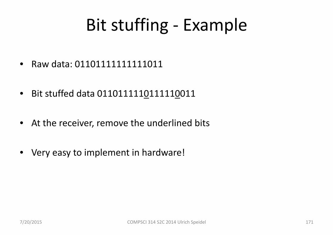
Bit stuffing ‐ Example
• Raw data: 01101111111111011
• Bit stuffed data 0110111110111110011
• At the receiver, remove the underlined bits
• Very easy to implement in hardware!
7/20/2015 COMPSCI 314 S2C 2014 Ulrich Speidel 172
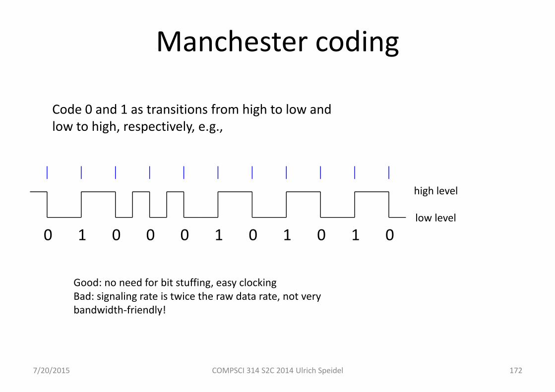
Manchester coding
Code 0 and 1 as transitions from high to low andlow to high, respectively, e.g.,
0 0 0 0 0 0 01 1 1 1low level
high level
Good: no need for bit stuffing, easy clockingBad: signaling rate is twice the raw data rate, not verybandwidth‐friendly!
7/20/2015 COMPSCI 314 S2C 2014 Ulrich Speidel 173
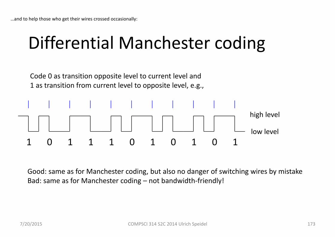
Differential Manchester coding
Code 0 as transition opposite level to current level and 1 as transition from current level to opposite level, e.g.,
1 1 1 1 1 1 10 0 0 0low level
high level
Good: same as for Manchester coding, but also no danger of switching wires by mistakeBad: same as for Manchester coding – not bandwidth‐friendly!
…and to help those who get their wires crossed occasionally:

Framing
• It is pretty common for communication channels to be idle –periods of time when nothing is transmitted
• When transmissions happen, they typically happen in the form of messages containing a certain number of bits or bytes. These messages are called frames– Depending on the context, they may also be called packets or datagrams etc.
• How do we know that nothing is transmitted (rather than just a long series of 0’s), and how do we recognise the start of a frame?
7/20/2015 COMPSCI 314 S2C 2014 Ulrich Speidel 174
Framing with bit stuffing and CRCs• A common approach (e.g., Ethernet) is to use bit stuffing
• Remember that in bit stuffing, the maximum number of consecutive 1‐bits we can get is 5
• Basic idea of framing: Mark the start and end of each frame by a byte 01111110 (six 1‐bits in series)
• Problem: Consider noise received between the end of a frame and the start of another. How does a receiver that has started listening during the last frame detect that the noise is not frame content?
– Note: The noise is preceded and followed by 01111110, too – the frame markers of the last and the next frame!
• Answer: protect each frame by including a CRC checksum and use the frame only if the CRC check is correct. Noise produces a random CRC checksum which is almost guaranteed to be wrong.
7/20/2015 COMPSCI 314 S2C 2014 Ulrich Speidel 175
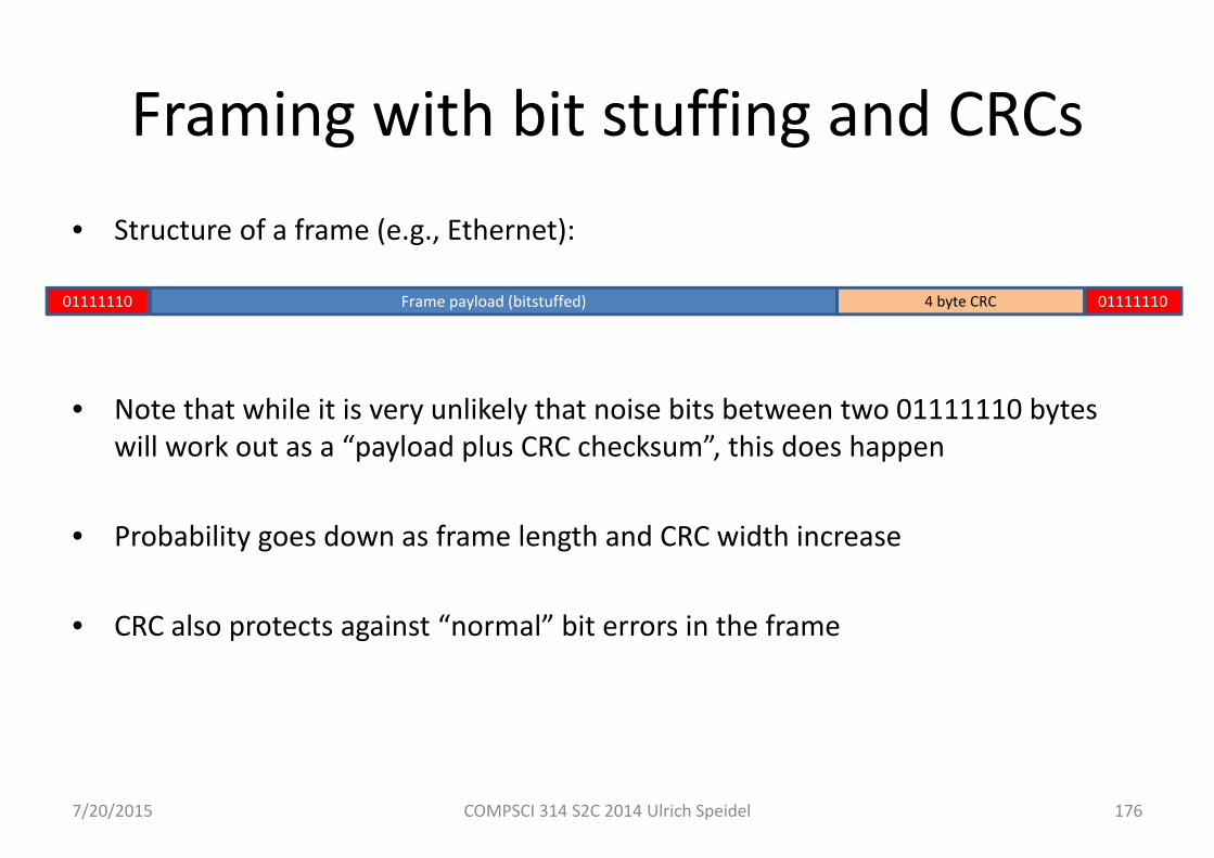
Framing with bit stuffing and CRCs• Structure of a frame (e.g., Ethernet):
• Note that while it is very unlikely that noise bits between two 01111110 bytes will work out as a “payload plus CRC checksum”, this does happen
• Probability goes down as frame length and CRC width increase
• CRC also protects against “normal” bit errors in the frame
7/20/2015 COMPSCI 314 S2C 2014 Ulrich Speidel 176
Frame payload (bitstuffed)01111110 011111104 byte CRC
Week 4
• Lecture 10: Data compression
• Lecture 11: Analog signals over digital channels
7/20/2015 COMPSCI 314 S2C 2014 Ulrich Speidel 177
Lecture 10
• Coding for efficiency: Data compression
• Huffman codes
• The Lempel‐Ziv 1978 algorithm (LZ78)
• Lossy compression
7/20/2015 COMPSCI 314 S2C 2014 Ulrich Speidel 178
7/20/2015 COMPSCI 314 S2C 2014 Ulrich Speidel 179
Coding again – under a Shannon‐Hartley perspective!
• Coding can help us to make the best of our bandwidth
• Hamming codes make us more robust against noise – at the expense of the payload bit rate!
• Shannon‐Hartley capacity really specifies a rate in “bits of information”, not necessarily binary digits– How many NRZ zero bits can you send per second? Infinitely many as long as
you don’t send any ones! On the other hand, do you send any information?
• Can use data compression to squeeze more real bits into our bits
7/20/2015 COMPSCI 314 S2C 2014 Ulrich Speidel 180
Data Compression with Variable‐Length Codes
• E.g., say we want to send messages composed from characters in the English alphabet, using a binary channel
• That is, we want to encode each letter in the English alphabet as a unique string of bits
• We also want this code to be uniquely decipherable, that is, no codeword must be a prefix of another! (e.g., A=101, B=1010 is not permitted!)
• Finally, we want the code to be efficient. In other words, we want a “typical” message to be as short as possible
• Can use a variable‐length code (VLC). E.g., assign short codewords to letters that appear frequently, and long codewords to letters that appear less often

7/20/2015 COMPSCI 314 S2C 2014 Ulrich Speidel 181
The ideal VLC
• If a letter x has the probability of occurrence P(x) and the encoding e(x) with length |e(x)|, then the ideal codeword length is |e(x)| = -log2(P(x))
• A typical message (where each letter occurs with its probability) is
ΣxP(x)|e(x)| = -Σx P(x) log2(P(x))
bits long
• Problem: in most practical cases, -log2(P(x)) is not an integer – so codewords of that length can’t exist!
• Also, we would like our code to be self‐synchronizing, i.e., if a bit is inverted, we would like to re‐establish decoding at the correct codeword boundaries as soon as possible!
7/20/2015 COMPSCI 314 S2C 2014 Ulrich Speidel 182
Practical VLCs
• Practical VLCs have some inefficiency in their coding – this is called the code’s redundancy:
r = ΣxP(x)|e(x)| + Σx P(x) log2(P(x))
where |e(x)| is the length of the actual encoding of x.
• Efficient coding means we need to try and minimize r.
Huffman codes• Huffman codes are one of the oldest data compression schemes – they’re from 1952.
They are built… using Huffman’s algorithm, which builds a Huffman tree
• Huffman’s algorithm assumes a source that emits symbols with a given probability, e.g., letters from the English alphabet, or certain measurement data values in a (long) series of measurements
• The probabilities of the source symbols / data values must be known (at least as estimates)
• Huffman codes are used, among other places, in some image and video formats (JPEG, MPEG‐2, MP3, …)
• Huffman codes are lossless, meaning we can recover the original data after decoding
7/20/2015 COMPSCI 314 S2C 2014 Ulrich Speidel 183
7/20/2015 COMPSCI 314 S2C 2014 Ulrich Speidel 184
Huffman’s Algorithm
• Huffman’s algorithm can be used to construct codes with minimum redundancy:
1. Sort all probabilities for the letters you wish to encode2. Combine the two lowest probabilities. Sort again. Repeat step 2 until only one
probability (=1) is left3. This gives you a tree4. Assign codewords by going into the tree, level by level, starting from the root
with an empty bit string.5. At each branching node (combined probability), add a 0 to the bit string for the
left branch, and a 1 for the right branch6. The strings assigned to the nodes at the bottom are the codewords
• Note: Huffman codes are not unique
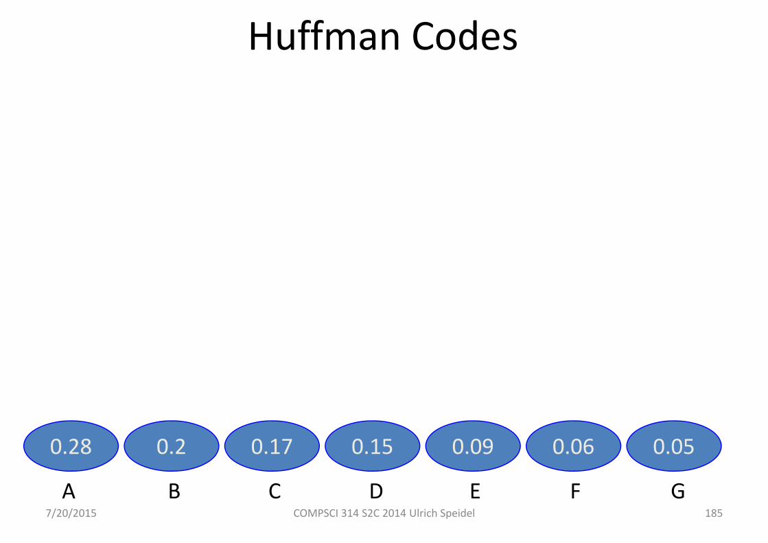
7/20/2015 COMPSCI 314 S2C 2014 Ulrich Speidel 185
Huffman Codes
0.28 0.2 0.17 0.15 0.09 0.06 0.05
A B C ED F G
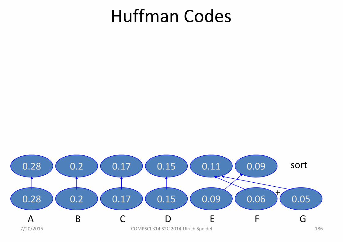
7/20/2015 COMPSCI 314 S2C 2014 Ulrich Speidel 186
0.28 0.2 0.17 0.15 0.09 0.06 0.05
0.11 0.090.150.28 0.2 0.17 sort
+
Huffman Codes
A B C ED F G
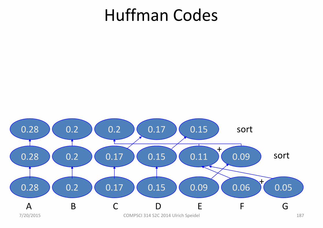
7/20/2015 COMPSCI 314 S2C 2014 Ulrich Speidel 187
0.28 0.2 0.17 0.15 0.09 0.06 0.05
0.11 0.090.150.28 0.2 0.17 sort
+
+
0.28 0.2 0.2 0.150.17 sort
Huffman Codes
A B C ED F G
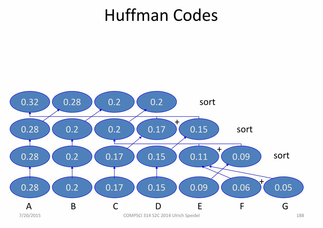
7/20/2015 COMPSCI 314 S2C 2014 Ulrich Speidel 188
0.28 0.2 0.17 0.15 0.09 0.06 0.05
0.11 0.090.150.28 0.2 0.17 sort
+
+
0.28 0.2 0.2 0.150.17 sort+
0.32 0.28 0.2 0.2 sort
Huffman Codes
A B C ED F G
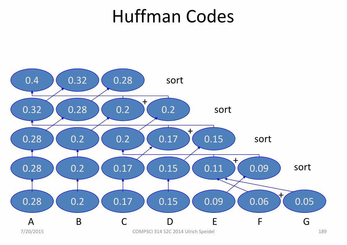
7/20/2015 COMPSCI 314 S2C 2014 Ulrich Speidel 189
0.28 0.2 0.17 0.15 0.09 0.06 0.05
0.11 0.090.150.28 0.2 0.17 sort
+
+
0.28 0.2 0.2 0.150.17 sort+
0.32 0.28 0.2 0.2 sort+
0.4 0.32 0.28 sort
Huffman Codes
A B C ED F G
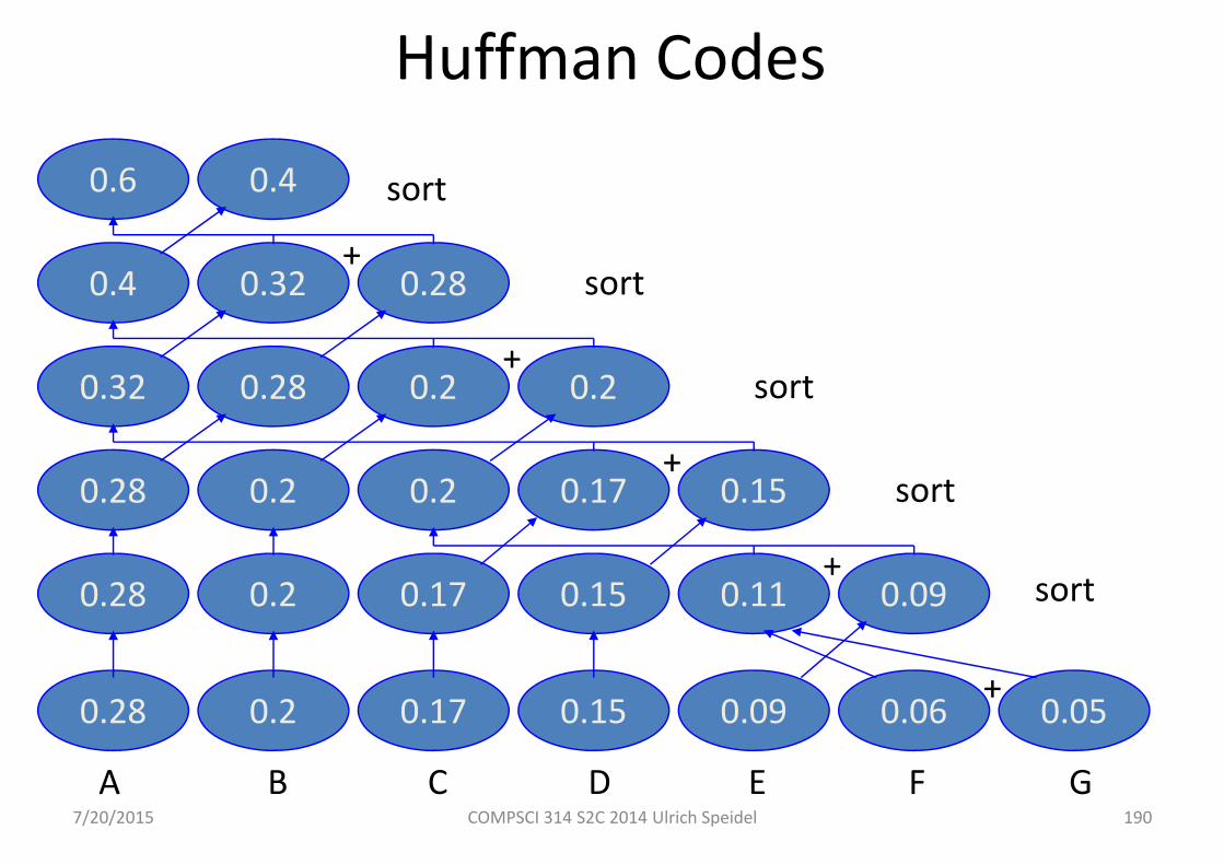
7/20/2015 COMPSCI 314 S2C 2014 Ulrich Speidel 190
0.28 0.2 0.17 0.15 0.09 0.06 0.05
0.11 0.090.150.28 0.2 0.17 sort
+
+
0.28 0.2 0.2 0.150.17 sort+
0.32 0.28 0.2 0.2 sort+
0.4 0.32 0.28 sort+
0.6 0.4 sort
Huffman Codes
A B C ED F G

7/20/2015 COMPSCI 314 S2C 2014 Ulrich Speidel 191
0.28 0.2 0.17 0.15 0.09 0.06 0.05
0.11 0.090.150.28 0.2 0.17 sort
+
+
0.28 0.2 0.2 0.150.17 sort+
0.32 0.28 0.2 0.2 sort+
0.4 0.32 0.28 sort+
0.6 0.4 sort
1 Huffman Codes+
A B C ED F G

7/20/2015 COMPSCI 314 S2C 2014 Ulrich Speidel 192
0.28 0.2 0.17 0.15 0.09 0.06 0.05
0.11 0.090.150.28 0.2 0.17 sort
+
+
0.28 0.2 0.2 0.150.17 sort+
0.32 0.28 0.2 0.2 sort+
0.4 0.32 0.28 sort+
0.6 0.4 sort
root Huffman Codes+
A B C ED F G

7/20/2015 COMPSCI 314 S2C 2014 Ulrich Speidel 193
0.28 0.2 0.17 0.15 0.09 0.06 0.05
0.11 0.090.150.28 0.2 0.17 sort
+
+
0.28 0.2 0.2 0.150.17 sort+
0.32 0.28 0.2 0.2 sort+
0.4 0.32 0.28 sort+
0 1 sort
root Huffman Codes+
A B C ED F G
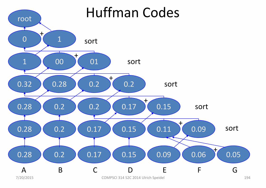
7/20/2015 COMPSCI 314 S2C 2014 Ulrich Speidel 194
0.28 0.2 0.17 0.15 0.09 0.06 0.05
0.11 0.090.150.28 0.2 0.17 sort
+
+
0.28 0.2 0.2 0.150.17 sort+
0.32 0.28 0.2 0.2 sort+
1 00 01 sort+
0 1 sort
root Huffman Codes+
A B C ED F G

7/20/2015 COMPSCI 314 S2C 2014 Ulrich Speidel 195
0.28 0.2 0.17 0.15 0.09 0.06 0.05
0.11 0.090.150.28 0.2 0.17 sort
+
+
0.28 0.2 0.2 0.150.17 sort+
00 01 10 11 sort+
1 00 01 sort+
0 1 sort
root Huffman Codes+
A B C ED F G

7/20/2015 COMPSCI 314 S2C 2014 Ulrich Speidel 196
0.28 0.2 0.17 0.15 0.09 0.06 0.05
0.11 0.090.150.28 0.2 0.17 sort
+
+
01 10 11 001000 sort+
00 01 10 11 sort+
1 00 01 sort+
0 1 sort
root Huffman Codes
A B C ED F G
+

7/20/2015 COMPSCI 314 S2C 2014 Ulrich Speidel 197
0.28 0.2 0.17 0.15 0.09 0.06 0.05
110 11100101 10 000 sort
+
+
01 10 11 001000 sort+
00 01 10 11 sort+
1 00 01 sort+
0 1 sort
root Huffman Codes+
A B C ED F G

7/20/2015 COMPSCI 314 S2C 2014 Ulrich Speidel 198
01 10 000 001 111 1100 1101
110 11100101 10 000 sort
+
+
01 10 11 001000 sort+
00 01 10 11 sort+
1 00 01 sort+
0 1 sort
root Huffman Codes+
A B C ED F G
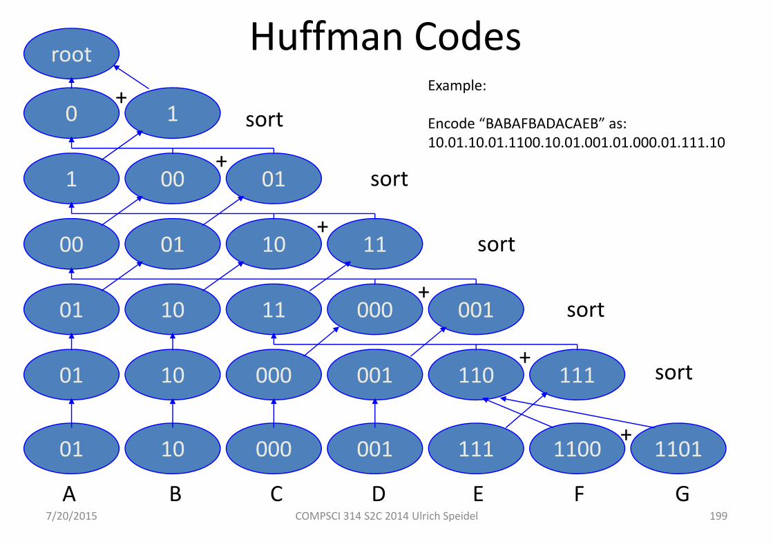
7/20/2015 COMPSCI 314 S2C 2014 Ulrich Speidel 199
01 10 000 001 111 1100 1101
110 11100101 10 000 sort
+
+
01 10 11 001000 sort+
00 01 10 11 sort+
1 00 01 sort+
0 1 sort
root Huffman Codes+
A B C ED F G
Example:
Encode “BABAFBADACAEB” as:10.01.10.01.1100.10.01.001.01.000.01.111.10

7/20/2015 COMPSCI 314 S2C 2014 Ulrich Speidel 200
Adaptive Huffman Coding
• Problem: we may know the number of different symbols that an information source may emit, but often don’t know their respective probabilities of occurrence
• E.g., may know that a source sends text but do not know how frequently certain letters (symbols) occur
• Can use adaptive Huffman coding:1. Start with using a block code (all symbols have equal probability)2. Send a symbol & compute source statistics for all symbols sent so far, both at the sender and at
the receiver3. Generate Huffman code for the new source probabilities at both ends. Use this Huffman code
for the next symbol4. Recompute statistics etc.
• Makes the assumption that upcoming symbols will be governed by the same probabilities as the previous ones
7/20/2015 COMPSCI 314 S2C 2014 Ulrich Speidel 201
Lempel‐Ziv compression (LZ78)
• One of a family of popular universal compression algorithms, developed by Abraham Lempel and Jacob Ziv
• Input: a string of bits. Output: an encoded tree (the vocabulary)
• Basic idea: – describe a bit string in a series of parsing steps– each step describes a substring as:
• a reference to an earlier substring, and• a one‐bit innovation
• The vocabulary is built as a tree, initially empty, with one node added at each step
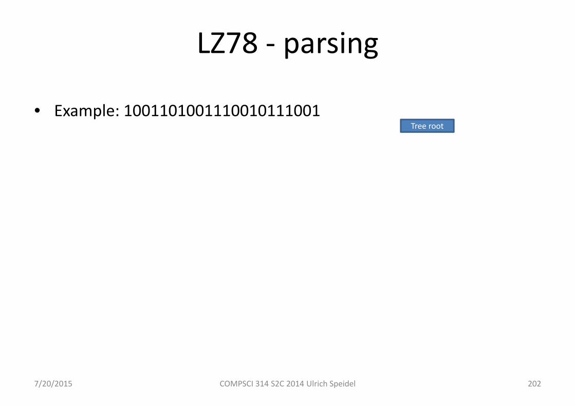
7/20/2015 COMPSCI 314 S2C 2014 Ulrich Speidel 202
LZ78 ‐ parsing
• Example: 1001101001110010111001Tree root
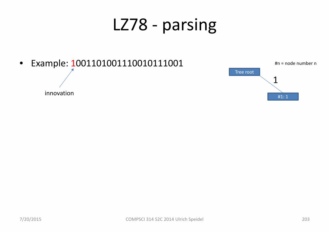
7/20/2015 COMPSCI 314 S2C 2014 Ulrich Speidel 203
LZ78 ‐ parsing
• Example: 1001101001110010111001Tree root
innovation
1#1: 1
#n = node number n
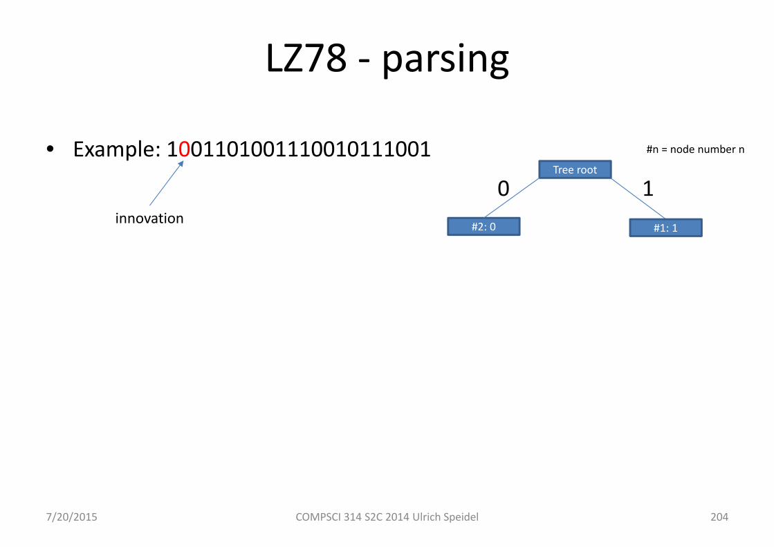
7/20/2015 COMPSCI 314 S2C 2014 Ulrich Speidel 204
LZ78 ‐ parsing
• Example: 1001101001110010111001Tree root
innovation
1#1: 1
0#2: 0
#n = node number n
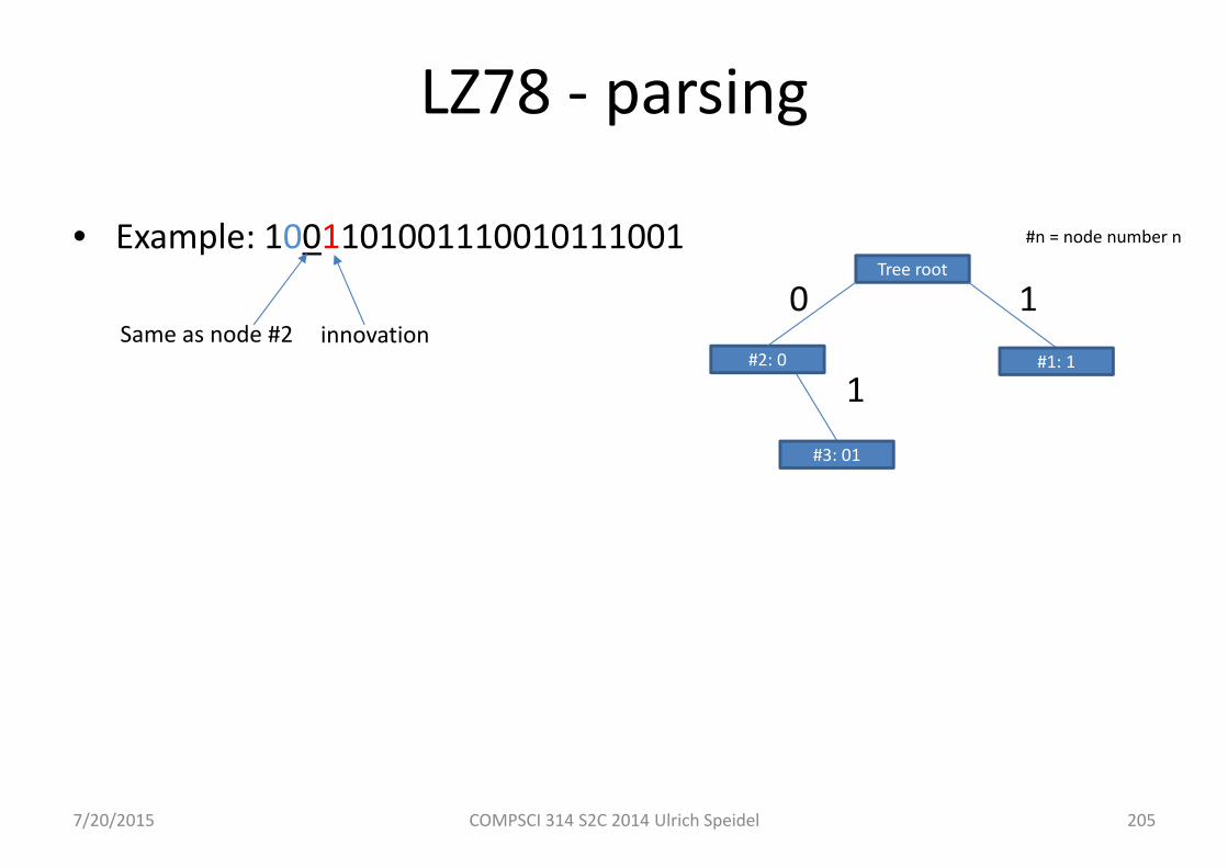
7/20/2015 COMPSCI 314 S2C 2014 Ulrich Speidel 205
LZ78 ‐ parsing
• Example: 1001101001110010111001Tree root
Same as node #21#1: 1
0#2: 0
innovation
1
#3: 01
#n = node number n
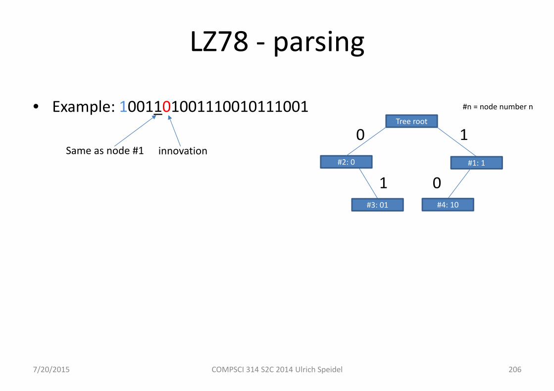
7/20/2015 COMPSCI 314 S2C 2014 Ulrich Speidel 206
LZ78 ‐ parsing
• Example: 1001101001110010111001Tree root
Same as node #11#1: 1
0#2: 0
innovation
1#3: 01
#n = node number n
0#4: 10
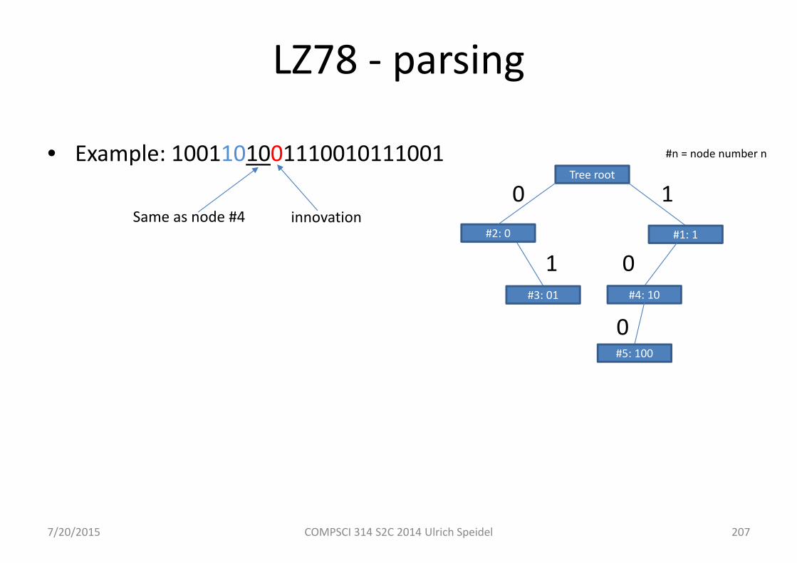
7/20/2015 COMPSCI 314 S2C 2014 Ulrich Speidel 207
LZ78 ‐ parsing
• Example: 1001101001110010111001Tree root
Same as node #41#1: 1
0#2: 0
innovation
1#3: 01
#n = node number n
0#4: 10
0#5: 100
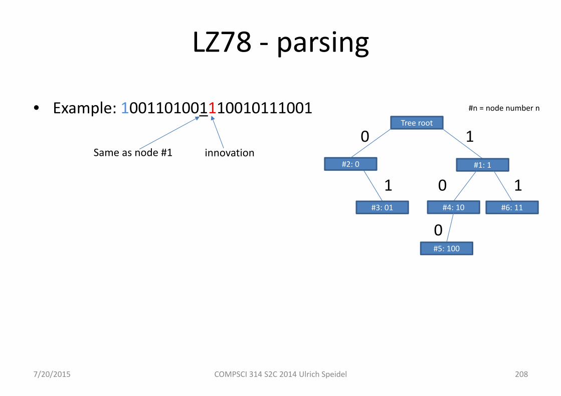
7/20/2015 COMPSCI 314 S2C 2014 Ulrich Speidel 208
LZ78 ‐ parsing
• Example: 1001101001110010111001Tree root
Same as node #11#1: 1
0#2: 0
innovation
1#3: 01
#n = node number n
0#4: 10
0#5: 100
1#6: 11

7/20/2015 COMPSCI 314 S2C 2014 Ulrich Speidel 209
LZ78 ‐ parsing
• Example: 1001101001110010111001Tree root
Same as node #51#1: 1
0#2: 0
innovation
1#3: 01
#n = node number n
0#4: 10
0#5: 100
1#6: 11
1#7: 1001
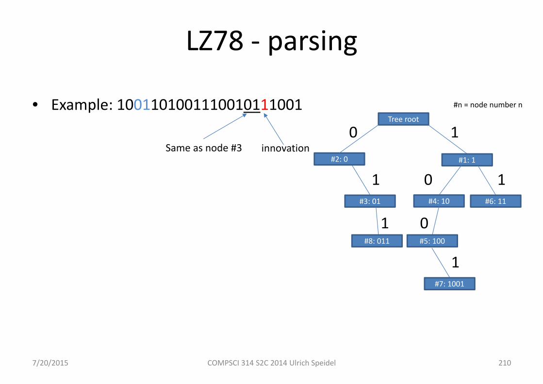
7/20/2015 COMPSCI 314 S2C 2014 Ulrich Speidel 210
LZ78 ‐ parsing
• Example: 1001101001110010111001Tree root
Same as node #31#1: 1
0#2: 0
innovation
1#3: 01
#n = node number n
0#4: 10
0#5: 100
1#6: 11
1#7: 1001
1#8: 011
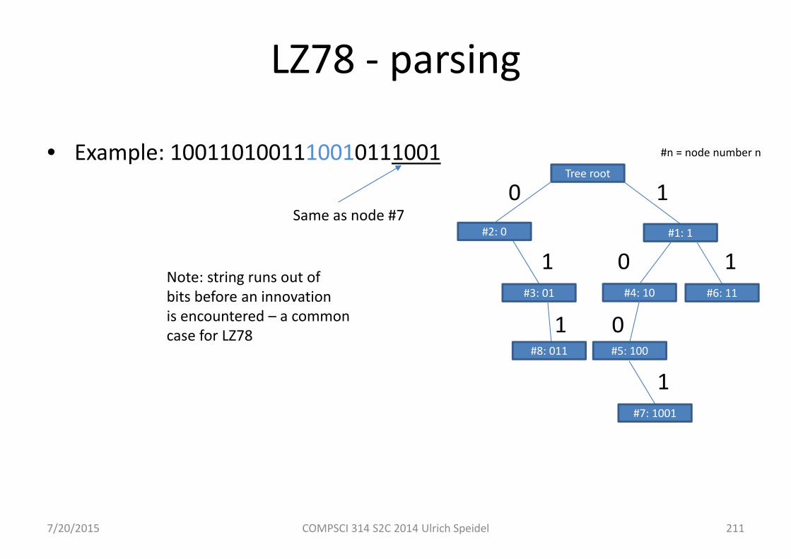
7/20/2015 COMPSCI 314 S2C 2014 Ulrich Speidel 211
LZ78 ‐ parsing
• Example: 1001101001110010111001Tree root
Same as node #71#1: 1
0#2: 0
1#3: 01
#n = node number n
0#4: 10
0#5: 100
1#6: 11
1#7: 1001
1#8: 011
Note: string runs out of bits before an innovationis encountered – a commoncase for LZ78
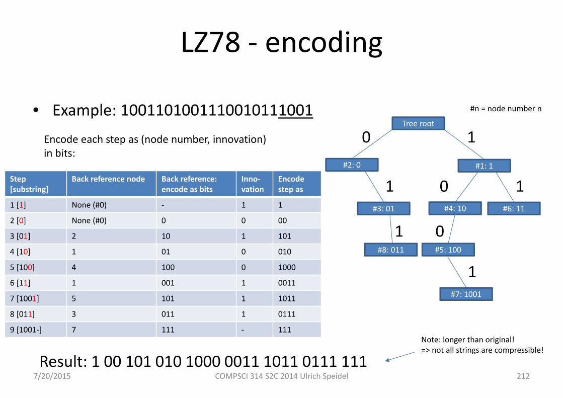
7/20/2015 COMPSCI 314 S2C 2014 Ulrich Speidel 212
LZ78 ‐ encoding
• Example: 1001101001110010111001Tree root
1#1: 1
0#2: 0
1#3: 01
#n = node number n
0#4: 10
0#5: 100
1#6: 11
1#7: 1001
1#8: 011
Encode each step as (node number, innovation)in bits:
Step [substring]
Back reference node Back reference: encode as bits
Inno‐vation
Encode step as
1 [1] None (#0) ‐ 1 1
2 [0] None (#0) 0 0 00
3 [01] 2 10 1 101
4 [10] 1 01 0 010
5 [100] 4 100 0 1000
6 [11] 1 001 1 0011
7 [1001] 5 101 1 1011
8 [011] 3 011 1 0111
9 [1001‐] 7 111 ‐ 111
Result: 1 00 101 010 1000 0011 1011 0111 111Note: longer than original!=> not all strings are compressible!
LZ‐78 comments
• LZ‐78 cannot compress all strings. It is best at compressing long strings which contain many repetitions of long substrings– our example did not, although you may have observed that the strings we
referenced got progressively a little longer
• Compression algorithms of the Lempel‐Ziv family (LZ‐78, LZ‐77, LZW etc.) are very widely used:– ZIP files (e.g., WinZip, Windows Compressed Folder, etc.)– .gz files (Linux gzip)– Frequently used to compress web pages on web servers before they are
transmitted to the browser – …plus many, many more applications
7/20/2015 COMPSCI 314 S2C 2014 Ulrich Speidel 213

Lecture 11
• Analog signals over digital channels
• Analog‐to‐digital conversion
7/20/2015 COMPSCI 314 S2C 2014 Ulrich Speidel 214
7/20/2015 COMPSCI 314 S2C 2014 Ulrich Speidel 215
Analog signals over digital channels
• E.g., telephony, video, but also remote measurement (telemetry)
• Need to convert analog values (voltages) to digital signals
• May not need all information in our analog signal

Digital voltage generator(D‐to‐A converter)‐ converts a number to a voltage
7/20/2015 COMPSCI 314 S2C 2014 Ulrich Speidel 216
Analog‐to‐Digital Conversion
Measuring devicelooks whether voltageat output is zero
Unknown voltage(e.g., from microphone)
Comparator(subtracts voltages)
Logic
Counter
Simple “ramp” ADC
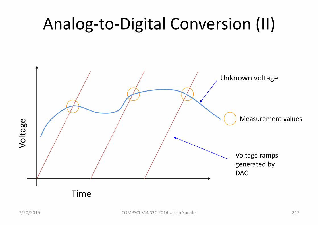
7/20/2015 COMPSCI 314 S2C 2014 Ulrich Speidel 217
Analog‐to‐Digital Conversion (II)
Unknown voltage
Volta
ge
Time
Voltage ramps generated by DAC
Measurement values
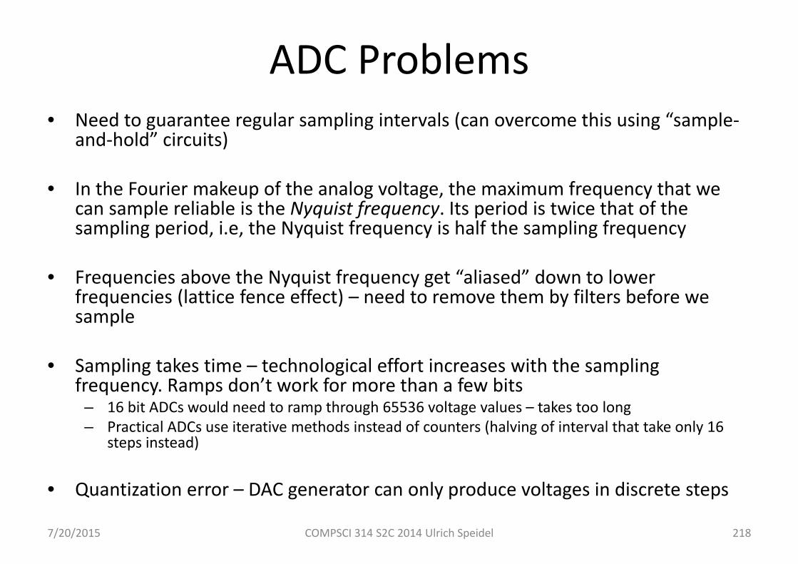
7/20/2015 COMPSCI 314 S2C 2014 Ulrich Speidel 218
ADC Problems• Need to guarantee regular sampling intervals (can overcome this using “sample‐
and‐hold” circuits)
• In the Fourier makeup of the analog voltage, the maximum frequency that we can sample reliable is the Nyquist frequency. Its period is twice that of the sampling period, i.e, the Nyquist frequency is half the sampling frequency
• Frequencies above the Nyquist frequency get “aliased” down to lower frequencies (lattice fence effect) – need to remove them by filters before we sample
• Sampling takes time – technological effort increases with the sampling frequency. Ramps don’t work for more than a few bits
– 16 bit ADCs would need to ramp through 65536 voltage values – takes too long– Practical ADCs use iterative methods instead of counters (halving of interval that take only 16
steps instead)
• Quantization error – DAC generator can only produce voltages in discrete steps
7/20/2015 COMPSCI 314 S2C 2014 Ulrich Speidel 219
Other ADC issues
• Sometimes, e.g., in audio and video applications, the intended “receiver” at the far end is a human being
• The human ear/eye usually cannot process all the information we can sample
• By leaving insignificant information out, we can still get the message across, but with far fewer bits (JPEG, MPEG, MP3, …)– This is called lossy compression
Lecture 12
• Revision/Overflow
7/20/2015 COMPSCI 314 S2C 2014 Ulrich Speidel 220