computability theory - springer
TRANSCRIPT
2Computability Theory
In this chapter we will develop a significant amount of computability theory.Much of this technical material will not be needed until much later in thebook, and perhaps in only a small section of the book. We have chosen togather it in one place for ease of reference. However, as a result this chapteris quite uneven in difficulty, and we strongly recommend that one use mostof it as a reference for later chapters, rather than reading through all of itin detail before proceeding. This is especially so for those unfamiliar withmore advanced techniques such as priority arguments.
In a few instances we will mention, or sometimes use, methods or resultsbeyond what we introduce in the present chapter. For instance, when wemention the work by Reimann and Slaman [327] on “never continuouslyrandom” sets in Section 6.12, we will talk about Borel Determinacy, andin a few places in Chapter 13, some knowledge of forcing in the contextof computability theory could be helpful, although our presentations willbe self-contained. Such instances will be few and isolated, however, andchoices had to be made to keep the length of the book somewhat withinreason.
2.1 Computable functions, coding, and the haltingproblem
At the heart of our understanding of algorithmic randomness is the notionof an algorithm. Thus the tools we use are based on classical computability
R.G. Downey and D. Hirschfeldt, Algorithmic Randomness and Complexity, Theory and 7Applications of Computability, DOI 10.1007/978-0-387-68441-3_2, © Springer Science+Business Media, LLC 2010

8 2. Computability Theory
theory. While we expect the reader to have had at least one course in therudiments of computability theory, such as a typical course on “theory ofcomputation”, the goal of this chapter is to give a reasonably self-containedaccount of the basics, as well as some of the tools we will need. We do,however, assume familiarity with the technical definition of computabilityvia Turing machines (or some equivalent formalism). For more details see,for example, Rogers [334], Salomaa [347], Soare [366], Odifreddi [310, 311],or Cooper [79].
Our initial concern is with functions from A into N where A ⊆ N, i.e.,partial functions on N. If A = N then the function is called total . Lookingonly at N may seem rather restrictive. For example, later we will be con-cerned with functions that take the set of finite binary strings or subsetsof the rationals as their domains and/or ranges. However, from the pointof view of classical computability theory (that is, where resources such astime and memory do not matter), our definitions naturally extend to suchfunctions by coding; that is, the domains and ranges of such functions canbe coded as subsets of N. For example, the rationals Q can be coded in Nas follows.
Definition 2.1.1. Let r ∈ Q \ {0} and write r = (−1)δ pq with p, q ∈ N in
lowest terms and δ = 0 or 1. Then define the Godel number of r, denotedby #(r), as 2δ3p5q. Let the Godel number of 0 be 0.
The function # is an injection from Q into N, and given n ∈ N wecan decide exactly which r ∈ Q, if any, has #(r) = n. Similarly, if σis a finite binary string, say σ = a1a2 . . . an, then we can define #(σ) =2a1+13a2+1 . . . (pn)an+1, where pn denotes the nth prime. There are myriadother codings possible, of course. For instance, one could code the stringσ as the binary number 1σ, so that, for example, the string 01001 wouldcorrespond to 101001 in binary. Coding methods such as these are called“effective codings”, since they include algorithms for deciding the resultinginjections, in the sense discussed above for the Godel numbering of therationals.
Henceforth, unless otherwise indicated, when we discuss computabilityissues relating to a class of objects, we will always regard these objects as(implicitly) effectively coded in some way.
Part of the philosophy underlying computability theory is the celebratedChurch-Turing Thesis, which states that the algorithmic (i.e., intuitivelycomputable) partial functions are exactly those that can be computed byTuring machines on the natural numbers. Thus, we formally adopt thedefinition of algorithmic, or computable, functions as being those that arecomputable by Turing machines, but argue informally, appealing to theintuitive notion of computability as is usual. Excellent discussions of thesubtleties of the Church-Turing Thesis can be found in Odifreddi [310] andSoare [367].

2.1. Computable functions, coding, and the halting problem 9
There are certain important basic properties of the algorithmic partialfunctions that we will use throughout the book, often implicitly. Followingthe usual computability theoretic terminology, we refer to such functionsas partial computable functions .
Proposition 2.1.2 (Enumeration Theorem – Universal Turing Machine).There is an algorithmic way of enumerating all the partial computablefunctions. That is, there is a list Φ0,Φ1, . . . of all such functions suchthat we have an algorithmic procedure for passing from an index i to aTuring machine computing Φi, and vice versa. Using such a list, we candefine a partial computable function f(x, y) of two variables such thatf(x, y) = Φx(y) for all x, y. Such a function, and any Turing machinethat computes it, are called universal.
To a modern computer scientist, this result is obvious. That is, given aprogram in some computer language, we can convert it into ASCII code,and treat it as a number. Given such a binary number, we can decodeit and decide whether it corresponds to the code of a program, and if soexecute this program. Thus a compiler for the given language can be usedto produce a universal program.
Henceforth, we fix an effective listing Φ0,Φ1, . . . of the partial computablefunctions as above. We have an algorithmic procedure for passing from anindex i to a Turing machine Mi computing Φi, and we identify each Φiwith Mi.
For any partial computable function f , there are infinitely many ways tocompute f . If Φy is one such algorithm for computing f , we say that y isan index for f .
The point of Proposition 2.1.2 is that we can pretend that we have allthe machines Φ1,Φ2, . . . in front of us. For instance, to compute 10 stepsin the computation of the 3rd machine on input 20, we can pretend towalk to the 3rd machine, put 20 on the tape, and run it for 10 steps (wewrite the result as Φ3(20)[10]). Thus we can computably simulate the actionof computable functions. In many ways, Proposition 2.1.2 is the platformthat makes undecidability proofs work, since it allows us to diagonalizeover the class of partial computable functions without leaving this class.For instance, we have the following result, where we write Φx(y)↓ to meanthat Φx is defined on y, or equivalently, that the corresponding Turingmachine halts on input y, and Φx(y) ↑ to mean that Φx is not defined ony.
Proposition 2.1.3 (Unsolvability of the halting problem). There is noalgorithm that, given x, y, decides whether Φx(y) ↓. Indeed, there is noalgorithm to decide whether Φx(x)↓.

10 2. Computability Theory
Proof. Suppose such an algorithm exists. Then by Proposition 2.1.2, itfollows that the following function g is (total) computable:
g(x) =
{1 if Φx(x)↑Φx(x) + 1 if Φx(x)↓ .
Again using Proposition 2.1.2, there is a y with g = Φy. Since g is total,g(y) ↓, so Φy(y) ↓, and hence g(y) = Φy(y) + 1 = g(y) + 1, which is acontradiction.
Note that we can define a partial computable function g via g(x) =Φx(x) + 1 and avoid contradiction, as it will follow that, for any indexy for g, we have Φy(y) ↑= g(y) ↑. Also, the reason for the use of partialcomputable functions in Proposition 2.1.2 is now clear: The argument aboveshows that there is no computable procedure to enumerate all (and only)the total computable functions.
Proposition 2.1.3 can be used to show that many problems are algorith-mically unsolvable by “coding” the halting problem into these problems.For example, we have the following result.
Proposition 2.1.4. There is no algorithm to decide whether the domainof Φx is empty.
To prove this proposition, we need a lemma, known as the s-m-n theorem.We state it for unary functions, but it holds for n-ary ones as well. Strictlyspeaking, the lemma below is the s-1-1 theorem. For the full statement andproof of the s-m-n theorem, see [366].
Lemma 2.1.5 (The s-m-n Theorem). Let g(x, y) be a partial computablefunction of two variables. Then there is a computable function s of onevariable such that, for all x, y,
Φs(x)(y) = g(x, y).
Proof. Given a Turing machine M computing g and a number x, we canbuild a Turing machine N that on input y simulates the action of writingthe pair (x, y) on M ’s input tape and running M . We can then find anindex s(x) for the function computed by N .
Proof of Proposition 2.1.4. We code the halting problem into the problemof deciding whether dom(Φx) = ∅. That is, we show that if we could decidewhether dom(Φx) = ∅ then we could solve the halting problem. Define apartial computable function of two variables by
g(x, y) =
{1 if Φx(x)↓↑ if Φx(x)↑ .
Notice that g ignores its second input.
2.2. Computable enumerability and Rice’s Theorem 11
Via the s-m-n theorem, we can consider g(x, y) as a computable collec-tion of partial computable functions. That is, there is a computable s suchthat, for all x, y,
Φs(x)(y) = g(x, y).
Now
dom(Φs(x)) =
{N if Φx(x)↓∅ if Φx(x)↑,
so if we could decide for a given x whether Φs(x) has empty domain, thenwe could solve the halting problem.
We denote the result of running the Turing machine corresponding to Φefor s many steps on input x by Φe(x)[s]. This value can of course be eitherdefined, in which case we write Φe(x)[s] ↓, or undefined, in which case wewrite Φe(x)[s]↑.
We will often be interested in the computability of families of functions.We say that f0, f1, . . . are uniformly (partial) computable if there is a (par-tial) computable function f of two variables such that f(n, x) = fn(x)for all n and x. It is not hard to see that f0, f1, . . . are uniformly partialcomputable iff there is a computable g such that fn = Φg(n) for all n.
2.2 Computable enumerability and Rice’s Theorem
We now show that the reasoning used in the proof of Proposition 2.1.4 canbe pushed much further. First we wish to regard all problems as coded bysubsets of N. For example, the halting problem can be coded by
∅′ = {x : Φx(x)↓}(or if we insist on the two-variable formulation, by {〈x, y〉 : Φx(y)↓}). Nextwe need some terminology.
Definition 2.2.1. A set A ⊆ N is called
(i) computably enumerable (c.e.) if A = dom(Φe) for some e, and
(ii) computable if A and A = N \A are both computably enumerable.
A set is co-c.e. if its complement is c.e. Thus a set is computable iffit is both c.e. and co-c.e. Of course, it also makes sense to say that Ais computable if its characteristic function χA is computable, particularlysince, as mentioned in Chapter 1, we identify sets with their characteristicfunctions. It is straightforward to check that A is computable in the senseof Definition 2.2.1 if and only if χA is computable.
We let We denote the eth computably enumerable set, that is, dom(Φe),and let We[s] = {x � s : Φe(x)[s] ↓}. We sometimes write We[s] as We,s.
12 2. Computability Theory
We think of We[s] as the result of performing s steps in the enumerationof We.
An index for a c.e. set A is an e such that We = A.We say that a family of sets A0, A1, . . . is uniformly computably enumer-
able if An = dom(fn) for a family f0, f1, . . . of uniformly partial computablefunctions. It is easy to see that this condition is equivalent to saying thatthere is a computable g such that An = Wg(n) for all n, or that there isa c.e. set A such that An = {x : 〈n, x〉 ∈ A} for all n. A family of setsA0, A1, . . . is uniformly computable if the functions χA0 , χA1 , . . . are uni-formly computable, which is equivalent to saying that both A0, A1, . . . andA0, A1, . . . are uniformly c.e.
Definition 2.2.1 suggests that one way to make a set A noncomputableis by ensuring that A is coinfinite and for all e, if We is infinite thenA∩We �= ∅. A c.e. set A with these properties is called simple. An infiniteset that contains no infinite c.e. set is called immune. (So a simple set isa c.e. set whose complement is immune.) Not all noncomputable c.e. setsare simple, since given any noncomputable c.e. set A, the set {2n : n ∈ A}is also c.e. and noncomputable, but is not simple.
The name computably enumerable comes from a notion of “effec-tively countable”, via the following characterization, whose proof isstraightforward.
Proposition 2.2.2. A set A is computably enumerable iff either A = ∅ orthere is a total computable function f from N onto A. (If A is infinite thenf can be chosen to be injective.)
Thus we can think of an infinite computably enumerable set as an effec-tively infinite list (but not necessarily in increasing numerical order). Notethat computable sets correspond to decidable questions, since if A is com-putable, then either A ∈ {∅,N} or we can decide whether x ∈ A as follows.Let f and g be computable functions such that f(N) = A and g(N) = A.Now enumerate f(0), g(0), f(1), g(1), . . . until x occurs (as it must). If xoccurs in the range of f , then x ∈ A; if it occurs in the range of g, thenx /∈ A.
It is straightforward to show that ∅′ is computably enumerable. Thus,by Proposition 2.1.3, it is an example of a computably enumerable set thatis not computable. As we will show in Proposition 2.4.5, ∅′ is a completecomputably enumerable set, in the sense that for any c.e. set A, there isan algorithm for computing A using ∅′. We will introduce another “highlyknowledgeable” real, closely related to ∅′ and denoted by Ω, in Definition3.13.6. Calude and Chaitin [48] pointed out that, in 1927, Emile Borelprefigured the idea of such knowledgeable reals by “defining” a real B suchthat the nth bit of B answers the nth question in an enumeration of allyes/no questions one can write down in French.
If A is c.e., then it clearly has a computable approximation, that is, a uni-formly computable family {As}s∈ω of sets such that A(n) = limsAs(n) for
2.3. The Recursion Theorem 13
all n. (For example, {We[s]}s∈ω is a computable approximation of We.) InSection 2.6, we will give an exact characterization of the sets that have com-putable approximations. In the particular case of c.e. sets, we can choosethe As so that A0 ⊆ A1 ⊆ A2 ⊆ · · · . In the constructions we discuss, when-ever we are given a c.e. set, we assume we have such an approximation, andthink of As as the set of numbers put into A by stage s of the construc-tion. In general, whenever we have an object X that is being approximatedduring a construction, we denote the stage s approximation to X by X [s].
An index set is a set A such that if x ∈ A and Φx = Φy then y ∈ A. Forexample, {x : dom(Φx) = ∅} is an index set. An index set can be thoughtof as coding a problem about computable functions (like the emptinessof domain problem) whose answer does not depend on the particular al-gorithm used to compute a function. Generalizing Proposition 2.1.4, wehave the following result, which shows that nontrivial index sets are nevercomputable. Its proof is very similar to that of Proposition 2.1.4.
Theorem 2.2.3 (Rice’s Theorem [332]). An index set A is computable(and so the problem it codes is decidable) iff A = N or A = ∅.
Proof. Let A /∈ {∅,N} be an index set. Let e be such that dom(Φe) = ∅.We may assume without loss of generality that e ∈ A (the case e ∈ A beingsymmetric). Fix i ∈ A. By the s-m-n theorem, there is a computable s(x)such that, for all y ∈ N,
Φs(x)(y) =
{Φi(y) if Φx(x)↓↑ if Φx(x)↑ .
If Φx(x)↓ then Φs(x) = Φi and so s(x) ∈ A, while if Φx(x)↑ then Φs(x) = Φeand so s(x) /∈ A. Thus, if A were computable, ∅′ would also be computable.
Of course, many nontrivial decision problems (such as the problem ofdeciding whether a natural number is prime, say) are not coded by indexsets, and so can have decidable solutions.
2.3 The Recursion Theorem
Kleene’s Recursion Theorem (also known as the Fixed Point Theorem)is a fundamental result in classical computability theory. It allows us touse an index for a computable function or c.e. set that we are building in aconstruction as part of that very construction. Thus it forms the theoreticalunderpinning of the common programming practice of having a routinemake recursive calls to itself.
Theorem 2.3.1 (Recursion Theorem, Kleene [209]). Let f be a total com-putable function. Then there is a number n, called a fixed point of f , such

14 2. Computability Theory
that
Φn = Φf(n),
and hence
Wn = Wf(n).
Furthermore, such an n can be computed from an index for f .
Proof. First define a total computable function d via the s-m-n Theoremso that
Φd(e)(k) =
{ΦΦe(e)(k) if Φe(e)↓↑ if Φe(e)↑ .
Let i be such that
Φi = f ◦ dand let n = d(i). Notice that Φi is total. The following calculation showsthat n is a fixed point of f .
Φn = Φd(i) = ΦΦi(i) = Φf◦d(i) = Φf(n).
The explicit definition of n given above can clearly be carried outcomputably given an index for f .
A longer but more perspicuous proof of the recursion theorem was givenby Owings [312]; see also Soare [366, pp. 36–37].
There are many variations on the theme of the recursion theorem, suchas the following one, which we will use several times below.
Theorem 2.3.2 (Recursion Theorem with Parameters, Kleene [209]). Letf be a total computable function of two variables. Then there is a totalcomputable function h such that Φh(y) = Φf(h(y),y), and hence Wh(y) =Wf(h(y),y), for all y. Furthermore, an index for h can be obtained effectivelyfrom an index for f .
Proof. The proof is similar to that of the recursion theorem. Let d be atotal computable function such that
Φd(x,y)(k) =
{ΦΦx(〈x,y〉)(k) if Φx(〈x, y〉)↓↑ if Φx(〈x, y〉)↑ .
Let i be such that
Φi(〈x, y〉) = f(d(x, y), y)
for all x and y, and let h(y) = d(i, y). Then
Φh(y) = Φd(i,y) = ΦΦi(〈i,y〉) = Φf(d(i,y),y) = Φf(h(y),y)
for all y. The explicit definition of h given above can clearly be carried outcomputably given an index for f .
2.4. Reductions 15
It is straightforward to modify the above proof to show that if f is a par-tial computable function of two variables, then there is a total computablefunction h such that Φh(y) = Φf(h(y),y) for all y such that f(h(y), y)↓.
In Section 3.5, we will see that there is a version of the recursion theoremfor functions computed by prefix-free machines, a class of machines thatwill play a key role in this book.
Here is a very simple application of the recursion theorem. We showthat ∅′ is not an index set. Let f be a computable function such thatΦf(n)(n) ↓ and Φf(n)(m) ↑ for all m �= n. Let n be a fixed point for f , sothat Φn = Φf(n). Let m �= n be another index for Φn. Then Φn(n) ↓ andhence n ∈ ∅′, but Φm(m) ↑ and hence m /∈ ∅′. So ∅′ is not an index set.Note that this example also shows that there is a Turing machine that haltsonly on its own index.
The following is another useful application of the recursion theorem.
Theorem 2.3.3 (Slowdown Lemma, Ambos-Spies, Jockusch, Shore, andSoare [7]). Let {Ue,s}e,s∈ω be a computable sequence of finite sets such thatUe,s ⊆ Ue,s+1 for all e and s. Let Ue =
⋃s Ue,s. There is a computable
function g such that for all e, s, n, we have Wg(e) = Ue and if n /∈ Ue,s thenn /∈Wg(e),s+1.
Proof. Let f be a computable function such that Wf(i,e) behaves as fol-lows. Given n, look for a least s such that n ∈ Ue,s. If such an s is found,ask whether n ∈ Wi,s. If not, then enumerate n into Wf(i,e). By the recur-sion theorem with parameters, there is a computable function g such thatWg(e) = Wf(g(e),e) for every e. If n /∈ Ue,s, then n /∈ Wg(e). If n ∈ Ue,s thenfor the least such s it cannot be the case that n ∈ Wg(e),s, since in thatcase we would have n /∈ Wf(g(e),e) = Wg(e). So n ∈ Wf(g(e),e) = Wg(e) butn /∈Wg(e),s.
We will provide the details of applications of versions of the recursiontheorem for several results in this chapter, but will assume familiarity withtheir use elsewhere in the book.
2.4 Reductions
The key concept used in the proof of Rice’s Theorem is that of reduction,that is, the idea that “if we can do B then this ability also allows us to doA”. In other words, questions about problem A are reducible to ones aboutproblem B. We want to use this idea to define partial orderings, known asreducibilities , that calibrate problems according to computational difficulty.The idea is to have A � B if the ability to solve B allows us also to solveA, meaning that B is “at least as hard as” A. In this section, we introduceseveral ways to formalize this notion, beginning with the best-known one,Turing reducibility. For any reducibility �R, we write A ≡R B, and say

16 2. Computability Theory
that A and B are R-equivalent , if A �R B and B �R A. We write A <R Bif A �R B and B �R A. Finally, we write A |R B if A �R B and B �R A.
2.4.1 Oracle machines and Turing reducibility
An oracle (Turing) machine is a Turing machine with an extra infinite read-only oracle tape, which it can access one bit at a time while performingits computation. If there is an oracle machine M that computes the set Awhen its oracle tape codes the set B, then we say that A is Turing reducibleto B, or B-computable, or computable in B, and write A �T B.1 Note that,in computing A(n) for any given n, the machine M can make only finitelymany queries to the oracle tape; in other words, it can access the value ofB(m) for at most finitely many m. The definition of relative computabilitycan be extended to functions in the obvious way. We will also considersituations in which the oracle tape codes a finite string. In that case, if themachine attempts to make any queries beyond the length of the string, thecomputation automatically diverges. All the notation we introduce belowfor oracle tapes coding sets applies to strings as well.
For example, let E = {x : dom(Φx) �= ∅}. In the proof of Proposition2.1.4, we showed that ∅′ �T E. Indeed the proof of Rice’s Theorem demon-strates that, for a nontrivial index set I, we always have ∅′ �T I. On theother hand, the unsolvability of the halting problem implies that ∅′ �T ∅.(Note that X �T ∅ iff X is computable. Indeed, if Y is computable, thenX �T Y iff X is computable.)
It is not hard to check that Turing reducibility is transitive and reflexive,and thus is a preordering on the subsets of N. The equivalence classes ofthe form deg(A) = {B : B ≡T A} code a notion of equicomputability andare called Turing degrees (of unsolvability), though we often refer to themsimply as degrees . We always use boldface lowercase letters such as a forTuring degrees. A Turing degree is computably enumerable if it contains acomputably enumerable set (which does not imply that all the sets in thedegree are c.e.). The Turing degrees inherit a natural ordering from Turingreducibility: a � b iff A �T B for some (or equivalently all) A ∈ a andB ∈ b. We will relentlessly mix notation by writing, for example, A <T b,for a set A and a degree b, to mean that A <T B for some (or equivalentlyall) B ∈ b.
The Turing degrees form an uppersemilattice. The join operation is in-duced by ⊕, where A ⊕ B = {2n : n ∈ A} ∪ {2n + 1 : n ∈ B}. ClearlyA,B �T A ⊕ B, and if A,B �T C, then A ⊕ B �T C. Furthermore, if
1We can also put resource bounds on our procedures. For example, if we count stepsand ask that computations halt in a polynomial (in the length of the input) number ofsteps, then we arrive at the polynomial time computable functions and the notion ofpolynomial time (Turing) reducibility. We will not consider such reducibilities here; seeAmbos-Spies and Mayordomo [10].
2.4. Reductions 17
A ≡T A and B ≡T B, then A⊕B ≡T A⊕ B. Thus it makes sense to definethe join a ∨ b of the degrees a and b to be the degree of A ⊕ B for some(or equivalently all) A ∈ a and B ∈ b. Kleene and Post [210] showed thatthe Turing degrees are not a lattice. That is, not every pair of degrees hasa greatest lower bound.
For sets A0, A1, . . ., let⊕
iAi = {〈i, n〉 : n ∈ Ai}. Note that, while Aj �T⊕iAi for all j, the degree of
⊕iAi may be much greater than the degrees
of the Ai’s. For instance, for any function f , we can let Ai = {f(i)}, inwhich case each Ai is a singleton, and hence computable, but
⊕iAi ≡T f .
We let 0 denote the degree of the computable sets. Note that each degreeis countable and has only countably many predecessors (since there are onlycountably many oracle machines), so there are continuum many degrees.
For an oracle machine Φ, we write ΦA for the function computed byΦ with oracle A (i.e., with A coded into its oracle tape). The analog ofProposition 2.1.2 holds for oracle machines. That is, there is an effectiveenumeration Φ0,Φ1, . . . of all oracle machines, and a universal oracle (Tur-ing) machine Φ such that ΦA(x, y) = ΦAx (y) for all x, y and all oraclesA.
We had previously defined Φe to be the eth partial computable func-tion. However, we have already identified partial computable functions withTuring machines, and we can regard normal Turing machines as oracle ma-chines with empty oracle tape; in fact it is convenient to identify the ethpartial computable function Φe with Φ∅
e. Thus there is no real conflict be-tween the two notations, and we will not worry about the double meaningof Φe.
When a set A has a computable approximation {As}s∈ω, we writeΦAe (n)[s] to mean the result of running Φe with oracle As on input n for smany steps.
We also think of oracle machines as determining (Turing) functionals ,that is, partial functions from 2ω to 2ω (or ωω). The value of the functionalΦ on A is ΦA.
The use of a converging oracle computation ΦA(n) is x+1 for the largestnumber x such that the value of A(x) is queried during the computation.(If no such value is queried, then the use of the computation is 0.) Wedenote this use by ϕA(n). In general, when we have an oracle computationrepresented by an uppercase Greek letter, its use function is representedby the corresponding lowercase Greek letter. Normally, we do not careabout the exact position of the largest bit queried during a computation,and can replace the exact use function by any function that is at least aslarge. Furthermore, we may assume that an oracle machine cannot queryits oracle’s nth bit before stage n. So we typically adopt the following usefulconventions on a use function ϕA.
1. The use function is strictly increasing where defined, that is, ϕA(m) <ϕA(n) for all m < n such that both these values are defined, and
18 2. Computability Theory
similarly, when A is being approximated, ϕA(m)[s] < ϕA(n)[s] for allm < n and s such that both these values are defined.
2. When A is being approximated, ϕA(n)[s] � ϕA(n)[t] for all n ands < t such that both these values are defined.
3. ϕA(n)[s] � s for all n and s such that this value is defined.
Although in a sense trivial, the following principle is quite important.
Proposition 2.4.1 (Use Principle). Let ΦA(n) be a converging oracle com-putation, and let B be a set such that B � ϕA(n) = A � ϕA(n). ThenΦB(n) = ΦA(n).
Proof. The sets A and B give the same answers to all questions askedduring the relevant computations, so the results must be the same.
One important consequence of the use principle is that if A is c.e. andΦA is total, then A can compute the function f defined by letting f(n) bethe least s by which the computation of ΦA(n) has settled, i.e., ΦA(n)[t]↓=ΦA(n)[s] ↓ for all t > s. The reason is that f(n) is the least s such thatΦA(n)[s]↓ and A � ϕA(n)[s] = As � ϕA(n)[s].
For a set A, let
A′ = {e : ΦAe (e)↓}.The set A′ represents the halting problem relativized to A. The generalprocess of extending a definition or result in the non-oracle case to theoracle case is known as relativization. For instance, Proposition 2.1.3 (theunsolvability of the halting problem) can be relativized with a completelyanalogous proof to show that A′ �T A for all A. Two good (but not hard)exercises are to show that A <T A′ and that if A �T B then A′ �T
B′. Another important example of relativization is the concept of a set Bbeing computably enumerable in a set A, which means that B = dom(ΦAe )for some e. Most results in computability theory can be relativized in acompletely straightforward way, and we freely use the relativized versionsof theorems proved below when needed.
2.4.2 The jump operator and jump classes
We often refer to A′ as the (Turing) jump of A. The jump operator is thefunction A → A′. The nth jump of A, written as A(n), is the result ofapplying the jump operator n times to A. So, for example, A(2) = A′′ andA(3) = A′′′. If a = deg(A) then we write a′ for deg(A′), and similarly for thenth jump notation. This definition makes sense because A ≡T B impliesA′ ≡T B
′. Note that we have a hierarchy of degrees 0 < 0′ < 0′′ < · · · .We also define the ω-jump of A as A(ω) =
⊕nA
(n). (We could continueto iterate the jump to define α-jumps for higher ordinals α, but we will notneed these in this book.)
2.4. Reductions 19
The halting problem, and hence the jump operator, play a fundamentalrole in much of computability theory. Closely connected to the jump opera-tor, and also of great importance in computability theory, are the followingjump classes .
Definition 2.4.2. A set A is lown if A(n) ≡T ∅(n). The low1 sets are calledlow .
A set A �T ∅′ is highn if A(n) ≡T ∅(n+1). The high1 sets are called high.More generally, we call an arbitrary set A high if A′ �T ∅′′.
These classes are particularly well suited to studying ∅′-computable sets.The following classes are sometimes better suited to the general case.
Definition 2.4.3. A set A is generalized lown (GLn) if A(n) ≡T (A ⊕∅′)(n−1).
A set A is generalized highn (GHn) if A(n) ≡T (A⊕ ∅′)(n).
Note that if A �T ∅′, then A is GLn iff it is lown, and GHn iff it is highn.A degree is low if the sets it contains are low, and similarly for other jumpclasses.
While jump classes are defined in terms of the jump operator, they oftenhave more “combinatorial” characterizations. For example, we will see inTheorem 2.23.7 that a set A is high iff there is an A-computable functionthat dominates all computable functions, where f dominates g if f(n) �g(n) for all sufficiently large n.
2.4.3 Strong reducibilities
The reduction used in the proof of Rice’s Theorem is of a particularlystrong type, since to decide whether x ∈ ∅′, we simply compute s(x) andask whether s(x) ∈ A. Considering this kind of reduction leads to thefollowing definition.
Definition 2.4.4. We say that A is many-one reducible (m-reducible) toB, and write A �m B, if there is a total computable function f such thatfor all x, we have x ∈ A iff f(x) ∈ B.2
If B is ∅ or N then the only set m-reducible to B is B itself, but we willignore these cases of the above definition. If the function f in the definitionof m-reduction is injective, then we say that A is 1-reducible to B, and
2In the context of complexity theory, resource bounded versions of m-reducibility areat the basis of virtually all modern NP-completeness proofs. Although Cook’s originaldefinition of NP-completeness was in terms of polynomial time Turing reducibility, theKarp version in terms of polynomial time m-reducibility is most often used. It is stillan open question of structural complexity theory whether there is a set A such that thepolynomial time Turing degree of A collapses to a single polynomial time m-degree.

20 2. Computability Theory
write A �1 B. Note that if B is c.e. and A �m B then A is also c.e. Alsonote that ∅′ is m-complete, and even 1-complete, in the following sense.
Proposition 2.4.5. If A is c.e. then A �1 ∅′.
Proof. It is easy to define an injective computable function f such that foreach n, the machine Φf(n) ignores its input and halts iff n enters A at somepoint. Then f witnesses the fact that A �1 ∅′.
It is not difficult to construct sets A and B such that A �T B butA �m B. For example, ∅′ �T ∅′, but ∅′ �m ∅′, since ∅′ is not c.e. It is alsopossible to construct such examples in which A and B are both c.e. Thusm-reducibility strictly refines Turing reducibility, and hence we say thatm-reducibility is an example of a strong reducibility (which should not beconfused with the notion of strong reducibility of mass problems introducedin Section 8.9). There are many other strong reducibilities. Their definitionsdepend on the types of oracle access used in the corresponding reductions.We mention two that will be important in this book.
One of the key aspects of Turing reducibility is that a Turing reductionmay be adaptable, in the sense that the number and type of queries made ofthe oracle depends upon the oracle itself. For instance, imagine a reductionthat works as follows: on input x, the oracle is queried as to whether itcontains some power of x. That is, the reduction asks whether 1 is in theoracle, then whether x is in the oracle, then whether x2 is in the oracle, andso on. If the answer is yes for some xn, then the reduction checks whetherthe least such n is even, in which case it outputs 0, or odd, in which caseit outputs 1.
Note that there is no limit to the number of questions asked of the oracleon a given input. This number depends on the oracle. Indeed, if the oraclehappens to contain no power of x, then the computation on input x willnot halt at all, and infinitely many questions will be asked.
Many naturally arising reductions do not have this adaptive property.One class of examples gives rise to the notion of truth table reducibility. Atruth table on the variables v1, v2, . . . is a (finite) boolean combination σ ofthese variables. We write A � σ if σ holds with vn interpreted as n ∈ A.For example, σ might be ((v1 ∧ v2) ∨ (v3 → v4)) ∧ v5), in which case A � σiff 5 ∈ A and either (1 ∈ A and 2 ∈ A) or (3 /∈ A or 4 ∈ A) (or both). Letσ0, σ1, . . . be an effective list of all truth tables.
Definition 2.4.6. We say that A is truth table reducible to B, and writeA �tt B, if there is a computable function f such that for all x,
x ∈ A iff B � σf(x).
Notice that an m-reduction is a simple example of a tt-reduction. Therelevant truth table for input n has a single entry vf(n), where f is thefunction witnessing the given m-reduction.
The following characterization follows easily from the compactness of 2ω.
2.4. Reductions 21
Proposition 2.4.7 (Nerode [293]). A Turing reduction Φ is a truth tablereduction iff ΦX is total for all oracles X.
This characterization is particularly useful in the context of effectivemeasure theory, as it means that truth table reductions can be used totransfer measures from one space to another. Examples can be found in thework of Reimann and Slaman [327, 328, 329] and the proof of Demuth’sTheorem 8.6.1 below.
Concepts defined using Turing reducibility often have productive analogsfor strong reducibilities. The following is an example we will use below.
Definition 2.4.8. A set A is superlow if A′ ≡tt ∅′.One way to look at a tt-reduction is that it is one in which the oracle
queries to be performed on a given input are predetermined, independentlyof the oracle, and the computation halts for every oracle. Removing thelast restriction yields the notion of weak truth table reduction, which canalso be thought of as bounded Turing reduction, in the sense that there is acomputable bound, independent of the oracle, on the amount of the oracleto be queried on a given input.
Definition 2.4.9. We say that A is weak truth table reducible (wtt-reducible) to B, and write A �wtt B, if there are a computable function fand an oracle Turing machine Φ such that ΦB = A and ϕB(n) � f(n) forall n.
Definitions and notations that we introduced for Turing reducibility, suchas the notion of degree, also apply to these strong reducibilities. In par-ticular, we have the notions of truth table functional and weak truth tablefunctional . For a Turing functional Φ to be a wtt-functional, we requirethat there be a single computable function f such that for all oracles B, ifΦB(n)↓ then ϕB(n) � f(n). The best way to think of a tt-functional is asa total Turing functional, that is, a functional Φ such that ΦB is total forall oracles B.
The reducibilities we have seen so far calibrate sets into degrees of greaterand greater fineness, in the order T, wtt, tt, m, 1.
2.4.4 Myhill’s Theorem
The definition of ∅′ depends on the choice of an effective enumeration ofthe partial computable functions. By Proposition 2.4.5, however, any twoversions of ∅′ are 1-equivalent. The following result shows that they are infact equivalent up to a computable permutation of N.
Theorem 2.4.10 (Myhill Isomorphism Theorem [291]). A ≡1 B iff thereis a computable permutation h of N such that h(A) = B.
Proof. The “if” direction is immediate, so assume that A �1 B via f andB �1 A via g. We define h in stages. We will ensure that the finite partial

22 2. Computability Theory
function hs defined at each stage is injective and such that m ∈ A iffhs(m) ∈ B for all m ∈ domhs.
Let h0 = ∅. Suppose we have defined hs for s even. Let m be least suchthat hs(m) is not defined. List f(n), f ◦h−1
s ◦f(n), f ◦h−1s ◦f ◦h−1
s ◦f(n), . . .until an element k /∈ rng hs is found. Note that each element of this list, andin particular k, is in B iff n ∈ A. Extend hs to hs+1 by letting hs+1(m) = k.
Now define hs+2 in the same way, with f , hs, dom, and rng replaced byg, h−1
s+1, rng, and dom, respectively.Let h =
⋃s hs. It is easy to check that h is a computable permutation of
N and that h(A) = B.
Myhill [291] characterized the 1-complete sets using the following notions.
Definition 2.4.11 (Post [316]). A set B is productive if there is a partialcomputable function h such that if We ⊆ B then h(e)↓∈ B \We.
A c.e. set A is creative if A is productive.
The halting problem is an example of a creative set, since ∅′ is productivevia the identity function.
Theorem 2.4.12 (Myhill’s Theorem [291]). The following are equivalentfor a set A.
(i) A is creative.
(ii) A is m-complete (i.e., m-equivalent to ∅′).
(iii) A is 1-complete (i.e., 1-equivalent to ∅′).
(iv) A is equivalent to ∅′ up to a computable permutation of N.
Proof. The Myhill Isomorphism Theorem shows that (iii) and (iv) areequivalent, and (iii) obviously implies (ii). To show that (ii) implies (i),suppose that ∅′ �m A via f . Let g be a computable function such thatWg(e) = {n : f(n) ∈ We} for all e, and let h(e) = f(g(e)). If We ⊆ A thenWg(e) ∈ ∅′, so g(e) ∈ ∅′\Wg(e), and hence h(e) ∈ A\We. Thus A is creativevia h.
To show that (i) implies (iii), we use the recursion theorem with param-eters. Since A is c.e., we have A �1 ∅′, so it is enough to show that ∅′ �1 A.Let h be a function witnessing that A is productive. Let f be a computablefunction such that Wf(n,k) = {f(n)} if k ∈ ∅′ and Wf(n,k) = ∅ otherwise.By the recursion theorem with parameters, there is an injective computablefunction g such that Wg(k) = Wf(g(k),k) for all k. Then
k ∈ ∅′ ⇒ Wg(k) = {f(g(k))} ⇒ Wg(k) � A ⇒ f(g(k)) ∈ A
and
k /∈ ∅′ ⇒ Wg(k) = ∅ ⇒ Wg(k) ⊆ A ⇒ f(g(k)) ∈ A.
Thus ∅′ �1 A via f ◦ g.

2.5. The arithmetic hierarchy 23
We will see a randomness-theoretic version of this result in Section 9.2.
2.5 The arithmetic hierarchy
We define the notions of Σ0n, Π0
n, and Δ0n sets as follows. A set A is Σ0
n ifthere is a computable relation R(x1, . . . , xn, y) such that y ∈ A iff
∃x1 ∀x2 ∃x3 ∀x4 · · ·Qnxn︸ ︷︷ ︸n alternating quantifiers
R(x1, . . . , xn, y).
Since the quantifiers alternate, Qn is ∃ if n is odd and ∀ if n is even. Inthis definition, we could have had n alternating quantifier blocks, insteadof single quantifiers, but we can always collapse two successive existentialor universal quantifiers into a single one by using pairing functions, so thatwould not make a difference.
The definition of A being Π0n is the same, except that the leading quan-
tifier is a ∀ (but there still are n alternating quantifiers in total). It is easyto see that A is Π0
n iff A is Σ0n.
Finally, we say a set is Δ0n if it is both Σ0
n and Π0n (or equivalently, if
both it and its complement are Σ0n). Note that the Δ0
0, Π00, and Σ0
0 sets areall exactly the computable sets. The same is true of the Δ0
1 sets, as shownby Proposition 2.5.1 below.
These notions give rise to Kleene’s arithmetic hierarchy, which can bepictured as follows.
Δ01 Δ0
2 Δ03 . . .
Σ01 Σ0
2
Π01 Π0
2
� �
� � �� �
� � �
A set is arithmetic if it is in one of the levels of the arithmetic hierarchy.As we will see in the next section, there is a strong relationship be-
tween the arithmetic hierarchy and enumeration. The following is a simpleexample at the lowest level of the hierarchy
Proposition 2.5.1 (Kleene [208]). A set A is computably enumerable iffA is Σ0
1.
Proof. Suppose A is c.e. Then A = dom(Φe) for some e, so n ∈ A iff∃sΦe(y)[s]↓. Thus A is Σ0
1.Conversely, if A is Σ0
1 then for some computable R we have n ∈ A iff∃xR(x, n). Define a partial computable function g by letting g(n) = 1 atstage s iff s � n and there is an x < s such that R(x, n) holds. Then n ∈ Aiff n ∈ dom(g), so A is c.e.

24 2. Computability Theory
2.6 The Limit Lemma and Post’s Theorem
There is an important generalization, due to Post, of Proposition 2.5.1. Itties in the arithmetic hierarchy with the degrees of unsolvability, and givescompleteness properties of degrees of the form 0(n), highlighting their im-portance. In this section we will look at this and related characterizations,beginning with Shoenfield’s Limit Lemma.
Saying that a set A is c.e. can be thought of as saying that A has a com-putable approximation that, for each n, starts out by saying that n /∈ A,and then changes its mind at most once. More precisely, there is a com-putable binary function f such that for all n we have A(n) = lims f(n, s),with f(n, 0) = 0 and f(n, s+ 1) �= f(n, s) for at most one s. Generalizingthis idea, the limit lemma characterizes the sets computable from the halt-ing problem as those that have computable approximations with finitelymany mind changes, and hence are “effectively approximable”. (In otherwords, the sets computable from ∅′ are exactly those that have computableapproximations, as defined in Section 2.2.)
Theorem 2.6.1 (Limit Lemma, Shoenfield [354]). For a set A, we haveA �T ∅′ iff there is a computable binary function g such that, for all n,
(i) lims g(n, s) exists (i.e., |{s : g(n, s) �= g(n, s+ 1)}| <∞), and
(ii) A(n) = lims g(n, s).
Proof. (⇒) Suppose A = Φ∅′. Define g by letting g(n, s) = 0 if either
Φ∅′[s] ↑ or Φ∅′
[s] ↓�= 1, and letting g(n, s) = 1 otherwise. Fix n, and let sbe a stage such that ∅′t � ϕ∅′
(n) = ∅′ � ϕ∅′(n) for all t � s. By the use
principle (Proposition 2.4.1), g(n, t) = Φ∅′(n)[t] = Φ∅′
(n) = A(n) for allt � s. Thus g has the required properties.
(⇐) Suppose such a function g exists. Without loss of generality, we mayassume that g(n, 0) = 0 for all n. To show that A �T ∅′, it is enough tobuild a c.e. set B such that A �T B, since by Proposition 2.4.5, every c.e.set is computable in ∅′. We put 〈n, k〉 into B whenever we find that
|{s : g(n, s) �= g(n, s+ 1)}| � k.
Now define a Turing reduction Γ as follows. Given an oracle X , on inputn, search for the least k such that 〈n, k〉 /∈ X , and if one is found, thenoutput 0 if k is even and 1 if k is odd. Clearly, ΓB = A.
As in the case of c.e. sets, whenever we are given a set A computable in∅′, we assume that we have a fixed computable approximation A0, A1, . . .to A; that is, we assume we have a computable function g as in the limitlemma, and write As for the set of all n such that g(n, s) = 1. We mayalways assume without loss of generality that A0 = ∅ and As ⊆ [0, s].
Intuitively, the proof of the “if” direction of the limit lemma boils downto saying that, since (by Propositions 2.4.5 and 2.5.1) the set ∅′ can decide

2.6. The Limit Lemma and Post’s Theorem 25
whether ∃s > t (g(n, s) �= g(n, s+ 1)) for any n and t, it can also computelims g(n, s).
Corollary 2.6.2. For a set A, the following are equivalent.
(i) A �tt ∅′.
(ii) A �wtt ∅′.
(iii) There are a computable binary function g and a computable functionh such that, for all n,
(a) |{s : g(n, s) �= g(n, s+ 1)}| < h(n), and(b) A(n) = lims g(n, s).
Proof. We know that (i) implies (ii). The proof that (ii) implies (iii) isessentially the same as that of the “if” direction of Theorem 2.6.1, togetherwith the remark that if Φ is a wtt-reduction then we can computably boundthe number of times the value of Φ∅′
[s] can change as s increases. The proofthat (iii) implies (i) is much the same as that of the “only if” direction ofTheorem 2.6.1, except that we can now make Γ into a tt-reduction becausewe have to check whether 〈n, k〉 /∈ X only for k < h(n).
Sets with the properties given in Corollary 2.6.2 are called ω-c.e., andwill be further discussed in Section 2.7.
As we have seen, we often want to relativize results, definitions, andproofs in computability theory. The limit lemma relativizes to show thatA �T B
′ iff there is a B-computable binary function f such that A(n) =lims f(n, s) for all n. Combining this fact with induction, we have thefollowing generalization of the limit lemma.
Corollary 2.6.3 (Limit Lemma, Strong Form, Shoenfield [354]). Let k �1. For a set A, we have A �T ∅(k) iff there is a computable function g ofk + 1 variables such that A(n) = lims1 lims2 . . . limsk
g(n, s1, s2, . . . , sk) forall n.
We now turn to Post’s characterization of the levels of the arithmetichierarchy. Let C be a class of sets (such as a level of the arithmetic hierar-chy). A set A is C-complete if A ∈ C and B �T A for all B ∈ C. If in factB �m A for all B ∈ C, then we say that A is C m-complete, and similarlyfor other strong reducibilities.
Theorem 2.6.4 (Post’s Theorem [317]). Let n � 0.
(i) A set B is Σ0n+1 ⇔ B is c.e. in some Σ0
n set ⇔ B is c.e. in some Π0n
set.
(ii) The set ∅(n) is Σ0n m-complete.
(iii) A set B is Σ0n+1 iff B is c.e. in ∅(n).
(iv) A set B is Δ0n+1 iff B �T ∅(n).

26 2. Computability Theory
Proof. (i) First note that if B is c.e. in A then B is also c.e. in A. Thus,being c.e. in a Σ0
n set is the same as being c.e. in a Π0n set, so all we need
to show is that B is Σ0n+1 iff B is c.e. in some Π0
n set.The “only if” direction has the same proof as the corresponding part of
Proposition 2.5.1, except that the computable relation R in that proof isnow replaced by a Π0
n relation R.For the “if” direction, let B be c.e. in some Π0
n set A. Then, byProposition 2.5.1 relativized to A, there is an e such that n ∈ B iff
∃s ∃σ ≺ A (Φσe (n)[s]↓). (2.1)
The property in parentheses is computable, while the property σ ≺ A isa combination of a Π0
n statement (asserting that certain elements are inA) and a Σ0
n statement (asserting that certain elements are not in A), andhence is Δ0
n+1. So (2.1) is a Σ0n+1 statement.
(ii) We proceed by induction. By Propositions 2.4.5 and 2.5.1, ∅′ is Σ01
m-complete. Now assume by induction that ∅(n) is Σ0n m-complete. Since
∅(n+1) is c.e. in ∅(n), it is Σ0n+1. Let C be Σ0
n+1. By part (i), C is c.e. in someΣ0n set, and hence it is c.e. in ∅(n). As in the unrelativized case, it is now
easy to define a computable function f such that n ∈ C iff f(n) ∈ ∅(n+1).(In more detail, let e be such that C = W ∅(n)
e , and define f so that for alloracles X and all n and x, we have ΦXf(n)(x)↓ iff n ∈WX
e .)(iii) By (i) and (ii), and the fact that if X is c.e. in Y and Y �T Z, then
X is also c.e. in Z.(iv) The set B is Δ0
n+1 iff B and B are both Σ0n+1, and hence both c.e.
in ∅(n) by (ii). But a set and its complement are both c.e. in X iff the setis computable in X . Thus B is Δ0
n+1 iff B �T ∅(n).
Note in particular that the Δ02 sets are exactly the ∅′-computable sets,
that is, the sets that have computable approximations.There are many “natural” sets, such as certain index sets, that are com-
plete for various levels of the arithmetic hierarchy. The following resultgives a few examples.
Theorem 2.6.5. (i) Fin = {e : We is finite} is Σ02 m-complete.
(ii) Tot = {e : Φe is total} and Inf = {e : We is infinite} are both Π02
m-complete.
(iii) Cof = {e : We is cofinite} is Σ03 m-complete.
Proof sketch. None of these are terribly difficult. We do (i) as an example.We know that ∅′′ is Σ0
2 m-complete by Post’s Theorem, and it is easy tocheck that Fin is itself Σ0
2, so it is enough to m-reduce ∅′′ to Fin. Using thes-m-n theorem, we can define a computable function f such that for all sand e, we have s ∈ Wf(e) iff there is a t � s such that either Φ∅′
e (e)[t]↑ or∅′t+1 � ϕ∅′
e (e)[t] �= ∅′t � ϕ∅′e (e)[t]. Then f(e) ∈ Fin iff Φ∅′
e (e)↓ iff e ∈ ∅′′.

2.7. The difference hierarchy 27
Part (ii) is similar, and (iii) is also similar but more intricate. See Soare[366] for more details.
2.7 The difference hierarchy
The arithmetic hierarchy gives us one way to extend the concept of com-putable enumerability. Another way to do so is via the difference hierarchy,which is defined as follows.
Definition 2.7.1. Let n � 1. A set A is n-computably enumerable (n-c.e.)if there is a computable binary function f such that for all x,
(i) f(x, 0) = 0,
(ii) A(x) = lims f(x, s), and
(iii) |{s : f(x, s+ 1) �= f(x, s)}| � n.
Thus the 1-c.e. sets are simply the c.e. sets. The 2-c.e. sets are often calledd.c.e., which stands for “difference of c.e.”, because of the easily proved factthat A is 2-c.e. iff there are c.e. sets B and C such that A = B \ C.
We have seen the following definition in Section 2.6.
Definition 2.7.2. A set A is ω-c.e. if there are a computable binaryfunction f and a computable unary function g such that for all x,
(i) f(x, 0) = 0,
(ii) A(x) = lims f(x, s), and
(iii) |{s : f(x, s+ 1) �= f(x, s)}| � g(x).
In Corollary 2.6.2, we saw that the ω-c.e. sets are exactly those that are(w)tt-reducible to ∅′. The following fact was probably known before it wasexplicitly stated by Arslanov [14].
Proposition 2.7.3 (Arslanov [14]). If A is ω-c.e. then there is a B ≡m Aand a computable binary function h such that for all x,
(i) h(x, 0) = 0,
(ii) B(x) = lims h(x, s), and
(iii) |{s : h(x, s+ 1) �= h(x, s)}| � x.
Proof. Let g be as in Definition 2.7.2. Without loss of generality, we mayassume that g is increasing. Let B = {g(x) : x ∈ A}. Then B clearly hasthe desired properties.
It is possible to define the concept of α-c.e. set for all computable ordi-nals α, forming what is known as the Ershov hierarchy. The details of thedefinition depend on ordinal notations. We will not use this concept in any

28 2. Computability Theory
significant way, so for simplicity we assume familiarity with the definitionof a computable ordinal and Kleene’s ordinal notations. For those unfamil-iar with these concepts, we refer to Rogers [334] and Odifreddi [310, 311].See Epstein, Haas, and Kramer [140] for more on α-c.e. sets and degrees.
Definition 2.7.4. Let α be a computable ordinal. A set A is α-c.e. relativeto a computable system S of notations for α if there is a partial computablefunction f such that for all x, we have A(x) = f(x, b) for the S-leastnotation b such that f(x, b) converges.
It is not hard to check that this definition agrees with the previous onesfor α � ω, independently of the system of notations chosen.
As in the c.e. case, we say that a degree is n-c.e. if it contains an n-c.e.set, and similarly for ω-c.e. and α-c.e. degrees.
2.8 Primitive recursive functions
The class of primitive recursive functions is the smallest class of functionssatisfying the following properties (where a 0-ary function is just a naturalnumber).
(i) The function n → n+ 1 is primitive recursive.
(ii) For each k and m, the function (n0, . . . , nk−1) → m is primitiverecursive.
(iii) For each k and i < k, the function (n0, . . . , nk−1) → ni is primitiverecursive.
(iv) If f and g0, . . . , gk−1 are primitive recursive, f is k-ary, and the gi areall j-ary, then
(n0, . . . , nj−1) → f(g0(n0, . . . , nj−1), . . . , gk−1(n0, . . . , nj−1))
is primitive recursive.
(v) If the k-ary function g and the (k + 2)-ary function h are primitiverecursive, then so is the function f defined by
f(0, n0, . . . , nk−1) = g(n0, . . . , nk−1)
and
f(i+ 1, n0, . . . , nk−1) = h(n, f(i, n0, . . . , nk−1), n0, . . . , nk−1).
It is easy to see that every primitive recursive function is computable.However, it is also easy to see that the primitive recursive functions aretotal and can be effectively listed, so there are computable functions that

2.9. A note on reductions 29
are not primitive recursive.3 A famous example is Ackermann’s function
A(m,n) =
⎧⎪⎨⎪⎩n+ 1 if m = 0A(m− 1, 1) if m > 0 ∧ n = 0A(m− 1, A(m,n− 1)) otherwise.
Many natural computable functions are primitive recursive, though, andit is sometimes useful to work with an effectively listable class of totalcomputable functions, so we will use primitive recursive functions in a fewplaces below.
2.9 A note on reductions
There are several ways to describe a reduction procedure. Formally, A �T
B means that there is an e such that ΦBe = A. In practice, though, wenever actually build an oracle Turing machine to witness the fact thatA �T B, but avail ourselves of the Church-Turing Thesis to informallydescribe a reduction Γ such that ΓB = A. One such description is givenin the proof of the ⇐ direction of Shoenfield’s Limit Lemma (Theorem2.6.1). This proof gives an example of a static definition of a reductionprocedure, in that the action of Γ is specified by a rule, rather than beingdefined during a construction. As an example of a dynamic definition of areduction procedure, we reprove the ⇐ direction of the limit lemma.
Recall that we are given a computable binary function g such that, forall n,
(i) lims g(n, s) exists and
(ii) A(n) = lims g(n, s).
We wish to show that A �T ∅′, by building a c.e. set B and a reductionΓB = A.
We simultaneously construct B and Γ in stages. We begin with B0 = ∅.For each n, we leave the value of ΓB(n) undefined until stage n. At stagen, we let ΓB(n)[n] = g(n, n) with use γB(n)[n] = 〈n, 0〉 + 1.
Furthermore, at stage s > 0 we proceed as follows for each n < s. Ifg(n, s) = g(n, s − 1), then we change nothing. That is, we let ΓB(n)[s] =ΓB(n)[s − 1] with the same use γB(n)[s] = γB(n)[s − 1]. Otherwise, weenumerate γ(n, s − 1) − 1 into B, which allows us to redefine ΓB(n)[s] =g(n, s), with use γB(n)[s] = 〈n, k〉 + 1 for the least 〈n, k〉 /∈ B.
It is not hard to check that ΓB = A, and that in fact this reduction isbasically the same as that in the original proof of the limit lemma (if we
3We can obtain the partial computable functions by adding to the five items abovean unbounded search scheme. See Soare [366] for more details and further discussion ofprimitive recursive functions.

30 2. Computability Theory
assume without loss of generality that g(n, n) = 0 for all n), at least as faras its action on oracle B goes.
More generally, the rules for a reduction ΔC to a c.e. set C are as follows,for each input n.
1. Initially ΔC(n)[0]↑.
2. At some stage s we must define ΔC(n)[s]↓= i for some value i, withsome use δC(n)[s]. By this action, we are promising that ΔC(n) = iunless C � δC(n)[s] �= Cs � δC(n)[s].
3. The convention now is that δC(n)[t] = δC(n)[s] for t > s unlessCt � δC(n)[s] �= Cs � δC(n)[t]. Should we find a stage t > s such thatCt � δC(n)[s] �= Cs � δC(n)[t], we then again have ΔC(n)[t]↑.
4. We now again must have a stage u � t at which we define ΔC(n)[u]↓=j for some value j, with some use δC(n)[u]. We then return to step3, with u in place of s.
5. If ΔC is to be total, we have to ensure that we stay at step 3 per-manently from some point on. That is, there must be a stage u atwhich we define ΔC(n)[u] and δC(n)[u], such that C � δC(n)[u] =Cu � δC(n)[u]. One way to achieve this is to ensure that, from somepoint on, whenever we redefine δC(n)[u], we set it to the same value.
In some constructions, C will be given to us, but in others we will buildit along with Δ. In this case, when we want to redefine the value of thecomputation ΔC(n) at stage s, we will often be able to do so by puttinga number less than δC(n)[s] into C (as we did in the limit lemma exampleabove).
There is a similar method of building a reduction ΔC when C is not c.e.,but merely Δ0
2. The difference is that now we must promise that if ΔC(n)[s]is defined and there is a t > s such that Ct � δC(n)[s] = Cs � δC(n)[s], thenΔC(n)[t] = ΔC(n)[s] and δC(n)[t] = δC(n)[s].
A more formal view of a reduction is as a partial computable map fromstrings to strings obeying certain continuity conditions. In this view, areduction ΓB = A is specified by a partial computable function f : 2<ω →2<ω such that
1. if σ ≺ B, then f(σ) ≺ A;
2. for all σ ≺ τ , if both f(σ)↓ and f(τ)↓, then f(σ) � f(τ); and
3. for all τ ≺ A there is a σ ≺ B such that τ ≺ f(σ).
The reduction in the proof of the ⇐ direction of the limit lemma can beviewed in this way by letting f(σ) be the longest string τ such that, for alln < |τ |, there is a k with σ(〈n, k〉) = 0, and τ(n) = 0 iff the first such k tobe found is even.

2.10. The finite extension method 31
Notice that this last method implies the following interesting observation:A function f : 2<ω → 2<ω is continuous iff it is computable relative to someoracle.
2.10 The finite extension method
In this section, we introduce one of the main techniques used in classicaldegree theory. We will refine this technique in the next section to what isknown as the finite injury priority method.
The dynamic construction of a reduction from B to A in the limit lemma,discussed in the previous section, has much in common with many proofsin classical computability theory. We perform a construction where someobject is built in stages. Typically, we have some overall goal that we breakdown into smaller subgoals that we argue are all met in the limit. In thiscase, the goal is to construct the reduction ΓB = A. We break this goal intothe subgoals of defining ΓB(n) for each n, and we accomplish these subgoalsby using the information supplied by our “opponent”, who is feeding usinformation about the universe, in this case the values g(n, s).
As an archetype for such proofs, think of Cantor’s proof that the col-lection of all infinite binary sequences is uncountable. One can conceive ofthis proof as follows. Suppose we could list the infinite binary sequencesas S = {S0, S1, . . .}, with Se = se,0se,1 . . . . It is our goal to construct abinary sequence U = u0u1 . . . that is not on the list S. We think of theconstruction as a game against our opponent who must supply us with S.We construct u in stages, at stage t specifying only u0 . . . ut, the initialsegment of U of length t+ 1. Our list of requirements is the decompositionof the overall goal into subgoals of the form
Re : U �= Se.
There is one such requirement for each e ∈ N. Of course, we know how tosatisfy these requirements. At stage e, we simply ensure that ue �= se,e bysetting ue = 1 − se,e. This action ensures that U �= Se for all e; in otherwords, all the requirements are met. This fact contradicts the assumptionthat S lists all infinite binary sequences, as U is itself an infinite binarysequence.
Notice that if we define a real number to be computable if it has a com-putable binary expansion, then the above proof can be used to show thatthere is no computable listing of all the computable reals (modulo someunimportant technicalities involving nonunique representations of reals).We will return to the topic of effective real numbers in Chapter 5.
Clearly, the proof of the unsolvability of the halting problem can also besimilarly recast, where this time the eth requirement asks us to invalidatethe eth member of some supposed list of all algorithms deciding whetherΦe(e)↓.

32 2. Computability Theory
While later results will be more complicated than these easy examples,the overall structure of the above should be kept in mind: Our constructionswill be in finite steps, where one or more objects are constructed stage bystage in finite pieces. These objects will be constructed to satisfy a list ofrequirements. The strategy we use will be dictated by how our opponentreveals the universe to us. Our overall goal is to satisfy all requirements inthe limit.
To finish this section, we look at a slightly more involved version of thistechnique. While we know that there are uncountably many Turing degrees,the only ones we have seen so far are the iterates of the halting problem.Rice’s Theorem 2.2.3 shows that all index sets are of degree � 0′. In 1944,Post [316] observed that all computably enumerable problems known at thetime were either computable or of Turing degree 0′. He asked the followingquestion.
Question 2.10.1 (Post’s Problem). Does there exist a computablyenumerable degree a with 0 < a < 0′?
As we will see in the next section, Post’s Problem was finally given apositive answer by Friedberg [161] and Muchnik [284], using a new andingenious method called the priority method. This method was an effec-tivization of an earlier method discovered by Kleene and Post [210]. Thelatter is called the finite extension method, and was used to prove thefollowing result.
Theorem 2.10.2 (Kleene and Post [210]). There are degrees a and b, bothbelow 0′, such that a | b. In other words, there are ∅′-computable sets thatare incomparable under Turing reducibility.4
Proof. We construct A = limsAs and B = limsBs in stages, to meet thefollowing requirements for all e ∈ N.
R2e : ΦAe �= B.
R2e+1 : ΦBe �= A.
Note that if A �T B then there must be some procedure Φe with ΦBe = A.Hence, if we meet all our requirements then A �T B, and similarly B �T A,so that A and B have incomparable Turing degrees. The fact that A,B �T
∅′ will come from the construction and will be observed at the end.The argument is by finite extensions, in the sense that at each stage s we
specify a finite portion As of A and a finite portion Bs of B. These finiteportions As and Bs will be specified as binary strings. The key invariantthat we need to maintain throughout the construction is that As � Au and
4The difference between the Kleene-Post Theorem and the solution to Post’s Prob-lem is that the degrees constructed in the proof of Theorem 2.10.2 are not necessarilycomputably enumerable, but merely Δ0
2.

2.10. The finite extension method 33
Bs � Bu for all stages u � s. Thus, after stage s we can only extend theportions of A and B that we have specified by stage s, which is a hallmarkof the finite extension method.Construction.Stage 0. Let A0 = B0 = λ (the empty string).Stage 2e+1. (Attend to R2e.) We will have specified A2e and B2e at stage2e. Pick some number x, called a witness , with x � |B2e|, and ask whetherthere is a string σ properly extending A2e such that Φσe (x)↓.
If such a σ exists, then let A2e+1 be the length-lexicographically leastsuch σ. Let B2e+1 be the string of length x + 1 extending B2e such thatB2e+1(n) = 0 for all n with |B2e| � n < x and B2e+1(x) = 1 − Φσe (x).
If no such σ exists, then let A2e+1 = A2e0 and B2e+1 = B2e0.Stage 2e+2. (Attend to R2e+1.) Define A2e+2 and B2e+2 by proceeding inthe same way as at stage 2e+ 1, but with the roles of A and B reversed.End of Construction.
Verification. First note that we have A0 ≺ A1 ≺ · · · and B0 ≺ B1 ≺ · · · ,so A and B are well-defined.
We now prove that we meet the requirement Rn for each n; in fact, weshow that we meet Rn at stage n+1. Suppose that n = 2e (the case wheren is odd being completely analogous). At stage n + 1, there are two casesto consider. Let x be as defined at that stage.
If there is a σ properly extending An with Φσe (x) ↓, then our action isto adopt such a σ as An+1 and define Bn+1 so that ΦAn+1
e (x) �= Bn+1(x).Since A extends An+1 and ΦAn+1
e (x)↓, it follows that A and An+1 agree onthe use of this computation, and hence ΦAe (x) = ΦAn+1
e . Since B extendsBn+1, we also have B(x) = Bn+1(x). Thus ΦAe (x) �= B(x), and Rn is met.
If there is no σ extending An with Φσe (x)↓, then since A is an extensionof An, it must be the case ΦA(x)↑, and hence Rn is again met.
Finally we argue that A,B �T ∅′. Notice that the construction is in factfully computable except for the decision as to which case we are in at a givenstage. There we must decide whether there is a convergent computation ofa particular kind. For instance, at stage 2e+1 we must decide whether thefollowing holds:
∃τ ∃s [τ � A2e ∧ Φτe (x)[s]↓]. (2.2)
This is a Σ01 question, uniformly in x, and hence can be decided by ∅′.5
The reasoning at the end of the above proof is quite common: we oftenmake use of the fact that ∅′ can answer any Δ0
2 question, and hence anyΣ0
1 or Π01 question.
5More precisely, we use the s-m-n theorem to construct a computable ternary functionf such that for all e, σ, x, and z, we have Φf(e,σ,x)(z)↓ iff (2.2) holds. Then (2.2) holdsiff f(e, σ, x) ∈ ∅′.
34 2. Computability Theory
A key ingredient of the proof of Theorem 2.10.2 is the use principle(Proposition 2.4.1). In constructions of this sort, where we build objectsto defeat certain oracle computations, a typical requirement will say some-thing like “the reduction Γ is not a witness to A �T B.” If we have aconverging computation ΓB(n)[s] �= A(n)[s] and we “preserve the use” ofthis computation by not changing B after stage s on the use γB(n)[s] (andsimilarly preserve A(n)), then we will preserve this disagreement. But thisuse corresponds to only a finite portion ofB, so we still have all the numbersbigger than it to meet other requirements. In the finite extension method,this use preservation is automatic, since once we define B(x) we never rede-fine it, but in other constructions we will introduce below, this may not bethe case, because we may have occasion to redefine certain values of B. Inthat case, to ensure that ΓB �= A, we will have to structure the constructionso that, if ΓB is total, then there are n and s such that ΓB(n)[s] �= A(n)[s]and, from stage s on, we preserve both A(n) and B � γB(n)[s].
2.11 Post’s Problem and the finite injury prioritymethod
A more subtle technique than the finite extension method is the prioritymethod . We begin by looking at the simplest incarnation of this eleganttechnique, the finite injury priority method . This method is somewhat likethe finite extension method, but with backtracking.
The idea behind it is the following. Suppose we must again satisfy re-quirements R0,R1, . . ., but this time we are constrained to some sort ofeffective construction, so we are not allowed to ask questions of a noncom-putable oracle during the construction. As an illustration, let us reconsiderPost’s Problem (Question 2.10.1). Post’s Problem asks us to find a c.e.degree strictly between 0 and 0′. It is clearly enough to construct c.e. setsA and B with incomparable Turing degrees. The Kleene-Post method doesallow us to construct sets with incomparable degrees below 0′, using a ∅′oracle question at each stage, but there is no reason to expect these sets tobe computably enumerable. To make A and B c.e., we must have a com-putable (rather than merely ∅′-computable) construction where elements gointo the sets A and B but never leave them. As we will see, doing so requiresgiving up on satisfying our requirements in order. The key idea, discoveredindependently by Friedberg [161] and Muchnik [284], is to pursue multiplestrategies for each requirement, in the following sense.
In the proof of the Kleene-Post Theorem, it appears that, in satisfyingthe requirement R2e, we need to know whether or not there is a σ extendingA2e such that Φσe (x) ↓, where x is our chosen witness. Now our idea is tofirst guess that no such σ exists, which means that we do nothing for R2e

2.11. Post’s Problem and the finite injury priority method 35
other than keep x out of B. If at some point we find an appropriate σ, wethen make A extend σ and put x into B if necessary, as in the Kleene-Postconstruction.
The only problem is that putting x into B may well upset the action ofother requirements of the form R2i+1, because such a requirement mightneed B to extend some string τ (for the same reason that R2e needs A toextend σ), which may no longer be possible. If we nevertheless put x intoB, we say that we have injured R2i+1. Of course, R2i+1 can now choose anew witness and start over from scratch, but perhaps another requirementmay injure it again later. So we need to somehow ensure that, for eachrequirement, there is a stage after which it is never injured.
To make sure that this is the case, we put a priority ordering on ourrequirements, by stating that Rj has stronger priority than Ri if j < i,and allow Rj to injure Ri only if Rj has stronger priority than Ri. ThusR0 is never injured. The requirement R1 may be injured by the action ofR0. However, once this happens R0 will never act again, so if R1 is allowedto start over at this point, it will succeed. This process of starting over iscalled initialization. Initializing R1 means that we restart its action witha new witness, chosen to be larger than any number previously seen in theconstruction, and hence larger than any number R0 cares about. This newincarnation of R1 is guaranteed never to be injured. It should now be clearthat, by induction, each requirement will eventually reach a point, followinga finite number of initializations, after which it will never be injured andhence will succeed in reaching its goal.
We may think of this kind of construction as a game between a teamof industrialists (each possibly trying to erect a factory) and a team ofenvironmentalists (each possibly trying to build a park). In the end wewant the world to be happy. In other words, we want all desired factoriesand parks to be built. However, some of the players may get distracted byother activities and never decide to build anything, so we cannot simplylet one player build, then the next, and so on, because we might then getpermanently stuck waiting for a player who never decides to build. Membersof the two teams have their own places in the pecking order. For instance,industrialist 6 has stronger priority than all environmentalists except thefirst six, and therefore can build anywhere except on parks built by thefirst six environmentalists. So industrialist 6 may choose to build on landalready demarcated by environmentalist 10, say, who would then need tofind another place to build a park. Of course, even if this event happens, ahigher ranked environmentalist, such as number 3, for instance, could laterlay claim to that same land, forcing industrialist 6 to find another placeto build a factory. Whether the highest ranked industrialist has priorityover the highest ranked environmentalist or vice versa is irrelevant to theconstruction, so we leave that detail to each reader’s political leanings.
For each player, there are only finitely many other players with strongerpriority, and once all of these have finished building what they desire, the

36 2. Computability Theory
given player has free pick of the remaining land (which is infinite), and canbuild on it without later being forced out.
In general, in a finite injury priority argument, we have a list of require-ments in some priority ordering. There are several different ways to meeteach individual requirement. Exactly which way will be possible to imple-ment depends upon information that is not initially available to us but is“revealed” to us during the construction. The problem is that a require-ment cannot wait for others to act, and hence must risk having its workdestroyed by the actions of other requirements. We must arrange thingsso that only requirements of stronger priority can injure ones of weakerpriority, and we can always restart the ones of weaker priority once theyare injured. In a finite injury argument, any requirement requires attentiononly finitely often, and we argue by induction that each requirement even-tually gets an environment wherein it can be met. As we will later see, thereare much more complex infinite injury arguments where one requirementmight injure another infinitely often, but the key there is that the injuryis somehow controlled so that it is still the case that each requirementeventually gets an environment wherein it can be met. Of course, imposingthis coherence criterion on our constructions means that each requirementmust ensure that its action does not prevent weaker requirements from find-ing appropriate environments (a principle known as Harrington’s “goldenrule”).
For a more thorough account of these beautiful techniques and their usesin modern computability theory, see Soare [366].
We now turn to the formal description of the solution to Post’s Problemby Friedberg and Muchnik, which was the first use of the priority method.In Chapter 11, we will return to Post’s Problem and explore its connectionswith the notion of Kolmogorov complexity.
Theorem 2.11.1 (Friedberg [161], Muchnik [284]). There exist computablyenumerable sets A and B such that A and B have incomparable Turingdegrees.
Proof. We build A =⋃sAs and B =
⋃sBs in stages to satisfy the same
requirements as in the proof of the Kleene-Post Theorem. That is, we makeA and B c.e. while meeting the following requirements for all e ∈ N.
R2e : ΦAe �= B.
R2e+1 : ΦBe �= A.
The strategy for a single requirement. We begin by looking at thestrategy for a single requirement R2e. We first pick a witness x to followR2e. This follower is targeted for B, and, of course, we initially keep it outof B. We then wait for a stage s such that ΦAe (x)[s] ↓= 0. If such a stagedoes not occur, then either ΦAe (x)↑ or ΦAe (x)↓�= 0. In either case, since wekeep x out of B, we have ΦAe (x) �= 0 = B(x), and hence R2e is satisfied.
2.11. Post’s Problem and the finite injury priority method 37
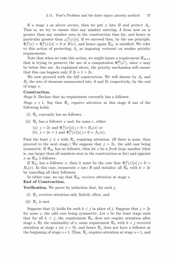
If a stage s as above occurs, then we put x into B and protect As.That is, we try to ensure that any number entering A from now on isgreater than any number seen in the construction thus far, and hence inparticular greater than ϕAe (x)[s]. If we succeed then, by the use principle,ΦAe (x) = ΦAe (x)[s] = 0 �= B(x), and hence again R2e is satisfied. We referto this action of protecting As as imposing restraint on weaker priorityrequirements.
Note that when we take this action, we might injure a requirement R2i+1
that is trying to preserve the use of a computation ΦBi (x′), since x maybe below this use. As explained above, the priority mechanism will ensurethat this can happen only if 2i+ 1 > 2e.
We now proceed with the full construction. We will denote by As andBs the sets of elements enumerated into A and B, respectively, by the endof stage s.Construction.Stage 0. Declare that no requirement currently has a follower.Stage s + 1. Say that Rj requires attention at this stage if one of thefollowing holds.
(i) Rj currently has no follower.
(ii) Rj has a follower x and, for some e, either
(a) j = 2e and ΦAe (x)[s]↓= 0 = Bs(x) or(b) j = 2e+ 1 and ΦBe (x)[s]↓= 0 = As(x).
Find the least j � s with Rj requiring attention. (If there is none, thenproceed to the next stage.) We suppose that j = 2e, the odd case beingsymmetric. If R2e has no follower, then let x be a fresh large number (thatis, one larger than all numbers seen in the construction so far) and appointx as R2e’s follower.
If R2e has a follower x, then it must be the case that ΦAe (x)[s] ↓= 0 =Bs(x). In this case, enumerate x into B and initialize all Rk with k > 2eby canceling all their followers.
In either case, we say that R2e receives attention at stage s.End of Construction.Verification. We prove by induction that, for each j,
(i) Rj receives attention only finitely often, and
(ii) Rj is met.
Suppose that (i) holds for each k < j in place of j. Suppose that j = 2efor some e, the odd case being symmetric. Let s be the least stage suchthat for all k < j, the requirement Rk does not require attention afterstage s. By the minimality of s, some requirement Rk with k < j receivedattention at stage s (or s = 0), and hence Rj does not have a follower atthe beginning of stage s+1. Thus, Rj requires attention at stage s+1, and

38 2. Computability Theory
is appointed a follower x. Since Rj cannot have its follower canceled unlesssome Rk with k < j receives attention, x is Rj ’s permanent follower.
It is clear by the way followers are chosen that x is never any otherrequirement’s follower, so x will not enter B unless Rj acts to put it intoB. So if Rj never requires attention after stage s+ 1, then x /∈ B, and wenever have ΦAe (x)[t] ↓= 0 for t > s, which implies that either ΦAe (x) ↑ orΦAe (x)↓�= 0. In either case, Rj is met.
On the other hand, if Rj requires attention at a stage t+1 > s+1, thenx ∈ B and ΦAe (x)[t]↓= 0. The only requirements that put numbers into Aafter stage t+1 are ones weaker than Rj (i.e., requirements Rk for k > j).Each such strategy is initialized at stage t + 1, which means that, whenit is later appointed a follower, that follower will be bigger than ϕAe (x)[t].Thus no number less than ϕAe (x)[t] will ever enter A after stage t+1, whichimplies, by the use principle, that ΦA(x) ↓= ΦAe (x)[t] = 0 �= B(x). So inthis case also, Rj is met. Since x ∈ Bt+2 and x is Rj ’s permanent follower,Rj never requires attention after stage t+ 1.
The above proof is an example of the simplest kind of finite injury ar-gument, what is called a bounded injury construction. That is, we canput a computable bound in advance on the number of times that a givenrequirement Rj will be injured. In this case, the bound is 2j − 1.
We give another example of this kind of construction, connected withthe important concept of lowness. It is natural to ask what can be saidabout the jump operator beyond the basic facts we have seen so far. Thenext theorem proves that the jump operator on degrees is not injective.Indeed, injectivity fails in the first place it can, in the sense that there arenoncomputable sets that the jump operator cannot distinguish from ∅.
Theorem 2.11.2 (Friedberg). There is a noncomputable c.e. low set.
Proof. We construct our set A in stages. To make A noncomputable weneed to meet the requirements
Pe : A �= We.
To make A low we meet the requirements
Ne : (∃∞sΦAe (e)[s]↓) ⇒ ΦAe (e)↓ .
To see that such requirements suffice, suppose they are met and definethe computable binary function g by letting g(e, s) = 1 if ΦAe (e)[s] ↓ andg(e, s) = 0 otherwise. Then g(e) = lims g(e, s) is well-defined, and by thelimit lemma, A′ = {e : g(e) = 1} �T ∅′.
The strategy for Pe is simple. We pick a fresh large follower x, and keepit out of A. If x enters We, then we put x into A. We meet Ne by anequally simple conservation strategy. If we see ΦAe (e)[s] ↓ then we simplytry to ensure that A � ϕAe (e)[s] = As � ϕAe (e)[s] by initializing all weakerpriority requirements, which forces them to choose fresh large numbers as

2.12. Finite injury arguments of unbounded type 39
followers. These numbers will be too big to injure the ΦAe (e)[s] computationafter stage s. The priority method sorts the actions of the various strategiesout. Since Pe picks a fresh large follower each time it is initialized, it cannotinjure any Nj for j < e. It is easy to see that any Ne can be injured atmost e many times, and that each Pe is met, since it is initialized at most2e many times.
Actually, the above proof constructs a noncomputable c.e. set that issuperlow. (Recall that a set A is superlow if A′ ≡tt ∅′.)
2.12 Finite injury arguments of unbounded type
2.12.1 The Sacks Splitting Theorem
There are priority arguments in which the number of injuries to each re-quirement, while finite, is not bounded by any computable function. Oneexample is the following proof of the Sacks Splitting Theorem [342]. Wewrite A = A0 � A1 to mean that A = A0 ∪ A1 and A0 ∩ A1 = ∅. Turingincomparable c.e. sets A0 and A1 such that A = A0 � A1 are said to forma c.e. splitting of A.
Theorem 2.12.1 (Sacks Splitting Theorem [342]). Every noncomputablec.e. set has a c.e. splitting.
Proof. Let A be a noncomputable c.e. set. We build Ai =⋃sAi,s in stages
by a priority argument to meet the following requirements for all e ∈ Nand i = 0, 1, while ensuring that A = A0 �A1.
Re,i : ΦAie �= A.
These requirements suffice because if A1−i �T Ai then A �T Ai.Without loss of generality, we assume that we are given an enumeration
of A so that exactly one number enters A at each stage. We must putthis number x ∈ As+1 \ As into exactly one of A0 or A1, to ensure thatA = A0 �A1.
To meet Re,i, we define the length of agreement function
l(e, i, s) = max{n : ∀k < n (ΦAie (k)[s] = A(k)[s])}
and an associated use function
u(e, i, s) = ϕAie (l(e, i, s) − 1)[s], 6
using the convention that use functions are monotone increasing (withrespect to the position variable) where defined.
6Of course, in defining this set we ignore s’s such that l(e, i, s) = 0. We will do thesame without further comment below. Here and below, we take the maximum of theempty set to be 0.

40 2. Computability Theory
The main idea of the proof is perhaps initially counterintuitive. Let usconsider a single requirement Re,i in isolation. At each stage s, althoughwe want ΦAi
e �= A, instead of trying to destroy the agreement betweenΦAie [s] and A[s] represented by l(e, i, s), we try to preserve it (a method
sometimes called the Sacks preservation strategy). The way we implementthis preservation is to put numbers entering A � u(e, i, s) after stage s intoA1−i and not into Ai. By the use principle, since this action freezes the Aiside of the computations involved in the definition of l(e, i, s), it ensuresthat ΦAi
e (k) = ΦAie (k)[s] for all k < l(e, i, s).
Now suppose that lim sups l(e, i, s) = ∞, so for each k we can findinfinitely many stages s at which k < l(e, i, s). For each such stage,ΦAie (k) = ΦAi
e (k)[s] = A(k)[s]. Thus A(k) = A(k)[s] for any such s. Sowe can compute A(k) simply by finding such an s, which contradicts thenoncomputability of A. Thus lim sups l(e, i, s) < ∞, which clearly impliesthat Re,i is met.
In the full construction, of course, we have competing requirements,which we sort out by using priorities. That is, we establish a priority list ofour requirements (for instance, saying that Re,i is stronger than Re′,i′ iff〈e, i〉 < 〈e′, i′〉). At stage s, for the single element xs entering A at stage s,we find the strongest priority Re,i with 〈e, i〉 < s such that xs < u(e, i, s)and put xs into A1−i. We say that Re,i acts at stage s. (If there is no suchrequirement, then we put xs into A0.)
To verify that this construction works, we argue by induction that eachrequirement eventually stops acting and is met. Suppose that all require-ments stronger than Re,i eventually stop acting, say by a stage s > 〈e, i〉. Atany stage t > s, if xt < u(e, i, t), then xt is put into A1−i. The same argu-ment as in the one requirement case now shows that if lim sups l(e, i, s) = ∞then A is computable, so lim sups l(e, i, s) < ∞. Our preservation strategythen ensures that lim sups u(e, i, s) < ∞. Thus Re,i eventually stops actingand is met.
In the above construction, injury to a requirement Re,i happens wheneverxs < u(e, i, s) but xs is nonetheless put into Ai, at the behest of a strongerpriority requirement. How often Re,i is injured depends on the lengths ofagreement attached to stronger priority requirements, and thus cannot becomputably bounded.
Note that, for any noncomputable c.e. set C, we can easily add require-ments of the form ΦAi
e �= C to the above construction, satisfying them inthe same way that we did for the Re,i. Thus, as shown by Sacks [342], inaddition to making A0 |T A1, we can also ensure that Ai �T C for i = 0, 1.
Note also that the computable enumerability of A is not crucial in theabove argument. Indeed, a similar argument works for any set A that hasa computable approximation, that is, any Δ0
2 set A. Such an argumentshows that if A and C are noncomputable Δ0
2 sets, then there exist Turingincomparable Δ0
2 sets A0 and A1 such that A = A0 � A1 and Ai �T C
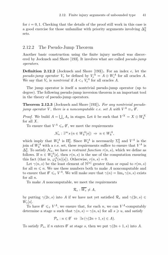
2.12. Finite injury arguments of unbounded type 41
for i = 0, 1. Checking that the details of the proof still work in this case isa good exercise for those unfamiliar with priority arguments involving Δ0
2
sets.
2.12.2 The Pseudo-Jump Theorem
Another basic construction using the finite injury method was discov-ered by Jockusch and Shore [193]. It involves what are called pseudo-jumpoperators.
Definition 2.12.2 (Jockusch and Shore [193]). For an index e, let thepseudo-jump operator Ve be defined by V Ae = A ⊕WA
e for all oracles A.We say that Ve is nontrivial if A <T V
Ae for all oracles A.
The jump operator is itself a nontrivial pseudo-jump operator (up todegree). The following pseudo-jump inversion theorem is an important toolin the theory of pseudo-jump operators.
Theorem 2.12.3 (Jockusch and Shore [193]). For any nontrivial pseudo-jump operator V , there is a noncomputable c.e. set A with V A ≡T ∅′.
Proof. We build A =⋃sAs in stages. Let k be such that V X = X ⊕WX
k
for all X .To ensure that V A �T ∅′, we meet the requirements
Nn : ∃∞s (n ∈ WAk [s]) ⇒ n ∈ WA
k ,
which imply that WAk is Π0
2. Since WAk is necessarily Σ0
2 and V A is thejoin of WA
k with a c.e. set, these requirements suffice to ensure that V A isΔ0
2. To satisfy Nn, we have a restraint function r(n, s), which we define asfollows. If n ∈ WA
k [s], then r(n, s) is the use of the computation ensuringthis fact (that is, ϕAk (n)[s]). Otherwise, r(n, s) = 0.
Let γ(n, s) be the least element of N[n] greater than or equal to r(m, s)for all m � n. We use these numbers both to make A noncomputable andto ensure that ∅′ �T V
A. We will make sure that γ(n) = lims γ(n, s) existsfor all n.
To make A noncomputable, we meet the requirements
Re : We �= A,
by putting γ(2e, s) into A if we have not yet satisfied Re and γ(2e, s) ∈We[s].
To have ∅′ �T V A, we ensure that, for each n, we can V A-computablydetermine a stage u such that γ(n, s) = γ(n, u) for all s � u, and satisfy
Pn : n ∈ ∅′ ⇔ ∃s (γ(2n+ 1, s) ∈ A).
To satisfy Pn, if n enters ∅′ at stage s, then we put γ(2n+ 1, s) into A.

42 2. Computability Theory
Thus the full construction proceeds as follows at stage s: For each e suchthat We[s] ∩A[s] = ∅ and γ(2e, s) ∈We[s], put γ(2e, s) into A. For each nentering ∅′ at stage s, put γ(2n+ 1, s) into A.
We put at most one number into A for the sake of a given R- or P-requirement. By the definition of the γ function, for each n there is an ssuch that, for all t � s, no number less than r(n, t) is put into A at staget. It follows that limt r(n, t) exists, and Nn is satisfied.
Thus γ(n) = lims γ(n, s) exists for all n, and the construction ensuresthat if We ∩A = ∅ then γ(2e) ∈ A iff γ(2e) ∈We, so that Re is satisfied.
It is also clear that each P-requirement is satisfied by the construction, sowe are left with showing that for each n, we can V A-computably determinea stage u such that γ(n, s) = γ(n, u) for all s � u. Assume by inductionthat we have determined a stage t such that γ(m, s) = γ(m, t) for all m < nand s � t. Let u > t be a stage such that for all m � n, if m ∈ WA
k thenm ∈WA
k [u]. Clearly, such a u can be found V A-computably. Let m � n. Ifm ∈ WA
k then r(m, s) = r(m,u) for all s � u, since no number less thanr(m,u) enters A during or after stage u. Now suppose that m /∈ WA
k . Foreach s � u, no number less than r(m, s) enters A during or after stage s, soif m were in WA
k [s] then it would be in WAk , and hence m /∈ WA
k [s]. Thusin this case r(m, s) = 0 for all s � u. So we see that r(m, s) = r(m,u) forall m � n and s � u, and hence γ(n, s) = γ(n, u) for all s � u.
Jockusch and Shore [193, 194] used the pseudo-jump machinery to estab-lish a number of results. One application is a finite injury proof that there isa high incomplete c.e. Turing degree, a result first proved using the infiniteinjury method, as we will see in Section 2.14.3. The Jockusch-Shore proof ofthe existence of a high incomplete c.e. degree in fact produces a superhighdegree (where a set X is superhigh if ∅′′ �tt X
′), and runs as follows. Rela-tivize the original Friedberg theorem that there is a noncomputable set We
of low (or even superlow) Turing degree, to obtain an operator Ve such thatfor all Y we have that Y <T V
Ye and V Ye is (super)low over Y . Then use
Theorem 2.12.3 to obtain a c.e. set A with V Ae ≡T ∅′. Then ∅′ is (super)lowover A and A <T ∅′, and hence A is (super)high and incomplete. We willuse this pseudo-jump technique again in Section 11.8. See Jockusch andShore [193, 194], Downey and Shore [132], and Coles, Downey, Jockusch,and LaForte [73] for more on the general theory of pseudo-jump operators.
2.13 Coding and permitting
Coding and permitting are two basic methods for controlling the degrees ofsets we build. Coding is a way of ensuring that a set A we build has degreeat least that of a given set B. As the name implies, it consists of encodingthe bits of B into A in a recoverable way. One simple way to to do this isto build A to equal B⊕C for some C, but in some cases we need to employ

2.13. Coding and permitting 43
a more elaborate coding method. We will see an example in Proposition2.13.1 below.
Permitting is a way of ensuring that a set A we build has degree at mostthat of a given set B. We will describe the basic form of c.e. permitting.For more elaborate forms of c.e. permitting, see Soare [366]. For a thoroughexposition of the Δ0
2 permitting method, see Miller [281].Let B be a noncomputable c.e. set, and suppose we are building a c.e.
set A to satisfy certain requirements while also ensuring that A �T B. Ata stage s in the construction, we may want to put a number n into A. Butinstead of putting n into A immediately, we wait for a stage t � s such thatBt+1 � n �= Bt � n. At that stage, we say that B permits us to put n intoA. If we always wait for permissions of this kind before putting numbersinto A, then we can compute A from B as follows. Given n, look for ans such that Bs � n = B � n. Then n ∈ A iff n ∈ As. Of course, one hasto worry whether a particular requirement can live with this permittingstrategy. But suppose that we have a requirement R that provides us withinfinitely many followers n, and will be satisfied as long as one such n entersA. Suppose that we never get a permission to put such an n into A. Thenwe can compute B as follows. Given m, wait for a stage s such that Rprovides us with a follower n > m. Since we are assuming we are neverpermitted to put n into A, we have B � n = Bs � n. In particular, m ∈ Biff m ∈ Bs. Since we are assuming that B is noncomputable, some followermust eventually be permitted to enter A, and hence R is satisfied.
The following proof illustrates both coding and permitting. Recall that acoinfinite c.e. set A is simple if its complement does not contain any infinitec.e. set.
Proposition 2.13.1. Every nonzero c.e. degree contains a simple set.
Proof. Let B be a noncomputable c.e. set. We may assume that exactlyone element xs enters B at each stage s. We build a c.e. set A ≡T B tosatisfy the simplicity requirements
Re : |We| = ∞ ⇒ We ∩A �= ∅.
At stage s, let as0 < as1 < · · · be the elements of As. For each e < s, ifWe,s ∩As = ∅ and there is an n ∈ We,s with n > 3e and n > xs, then putn into A. Also, put as3xs
into A.The set A is clearly c.e. Each Re puts at most one number into A, and
this number must be greater than 3e, while for each x ∈ B, the coding ofB puts only one number into A, and this number is at least 3x. Thus A iscoinfinite.
For each n, if Bs � n + 1 = B � n + 1, then n < xt for all t > s, so ncannot enter A after stage s. As explained above, it follows that A �T B.
Given x, the set A can compute a stage s such that asi ∈ A for all i � 3x.Then at3x = as3x for all t � s, so x ∈ B iff either x ∈ Bs or as3x ∈ A. ThusB �T A.

44 2. Computability Theory
Finally, we need to show that each Re is met. Suppose that We is infinitebut We ∩ A = ∅. Then we can computably find 3e < n0 < n1 < · · · ande � s0 < s1 < · · · such that ni ∈ We,si for all i. None of the ni are everpermitted by B, that is, ni � xt for all i and t � si. So B � ni = Bsi � nifor all i, and hence B is computable, contrary to hypothesis. Thus eachrequirement is met, and hence A is simple.
2.14 The infinite injury priority method
In this section, we introduce the infinite injury priority method. We beginby discussing the concept of priority trees, then give a few examples ofconstructions involving such trees. See Soare [366] for further examples.
2.14.1 Priority trees and guessing
The Friedberg-Muchnik construction used to prove Theorem 2.11.1 can beviewed another way. Instead of having a single strategy for each require-ment, which is restarted every time a stronger priority requirement acts,we can attach multiple versions of each requirement to a priority tree, inthis case the full binary tree 2<ω.
Recall that the relevant requirements are the following.
R2e : ΦAe �= B.
R2e+1 : ΦBe �= A.
Attached to each node σ is a “version” Rσ of R|σ|. We call such a versiona strategy for R|σ|, and refer to σ itself as a guess , for reasons that willsoon become clear. Thus there are 2e separate strategies for Re.
Each strategy Rσ has two outcomes , 0 and 1. The outcome 1 indicatesthat Rσ appoints a follower but never enumerates this follower into itstarget set. The outcome 0 indicates that Rσ actually enumerates its followerinto its target set. At a stage s, we have a guess as to which outcome iscorrect, depending on whether or not Rσ has enumerated its follower intoits target set. If this guess is ever 0, then we immediately know that 0 isindeed the correct outcome, so we regard the 0 outcome as being strongerthan the 1 outcome. We order our guesses lexicographically, and hence if σis to the left of τ , then we think of σ as being stronger than τ .
Figure 2.1 shows the above setup. For comparison, it also shows thesetup for the Minimal Pair Theorem, which will be discussed in the nextsubsection.
Here is how this mechanism is used. Consider R1. We have two strategiesfor this requirement. One, which in this paragraph we write as R〈0〉 ratherthan R0 to avoid confusion with R0, is below the 0 outcome of Rλ andthe other, R〈1〉, is below the 1 outcome of Rλ. We think of these versions
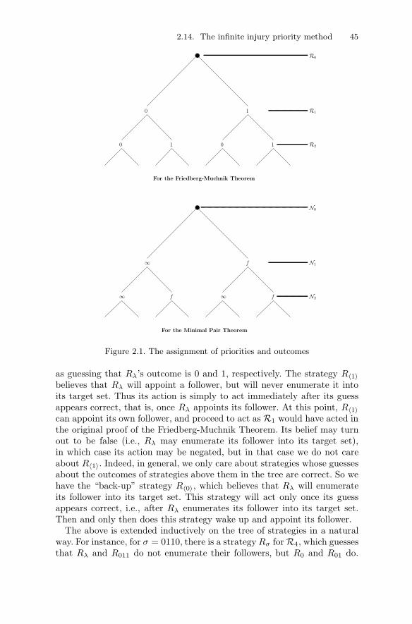
2.14. The infinite injury priority method 45
For the Minimal Pair Theorem
0
1 1
1
0 0
R0
R2
R1
For the Friedberg-Muchnik Theorem
N0
N1
N2
∞
∞ ∞f
f
f
Figure 2.1. The assignment of priorities and outcomes
as guessing that Rλ’s outcome is 0 and 1, respectively. The strategy R〈1〉believes that Rλ will appoint a follower, but will never enumerate it intoits target set. Thus its action is simply to act immediately after its guessappears correct, that is, once Rλ appoints its follower. At this point, R〈1〉can appoint its own follower, and proceed to act as R1 would have acted inthe original proof of the Friedberg-Muchnik Theorem. Its belief may turnout to be false (i.e., Rλ may enumerate its follower into its target set),in which case its action may be negated, but in that case we do not careabout R〈1〉. Indeed, in general, we only care about strategies whose guessesabout the outcomes of strategies above them in the tree are correct. So wehave the “back-up” strategy R〈0〉, which believes that Rλ will enumerateits follower into its target set. This strategy will act only once its guessappears correct, i.e., after Rλ enumerates its follower into its target set.Then and only then does this strategy wake up and appoint its follower.
The above is extended inductively on the tree of strategies in a naturalway. For instance, for σ = 0110, there is a strategyRσ for R4, which guessesthat Rλ and R011 do not enumerate their followers, but R0 and R01 do.
46 2. Computability Theory
This strategy waits for Rλ and R011 to appoint followers, and for R0 andR01 to both appoint followers and then enumerate them. Once all of theseconditions are met, it appoints its own follower and proceeds to act as R4
would have acted in the original proof of the Friedberg-Muchnik Theorem.More precisely, at stage s, we have a guess σs of length s, which is defined
inductively. Only those strategies Rτ with τ � σs get to act at stage s. Wesay that such τ are visited at stage s. Suppose we have defined σs � n. Letτ = σs � n. Then we allow Rτ to act as follows. Let us suppose that n = 2e,the odd case being symmetric. If Rτ has previously put a number into B,then it does nothing. In this case, if n < s then σ(n) = 0. Otherwise, Rτacts in one of three ways.
1. If Rτ does not currently have a follower, then it appoints a followerxτ greater than any number seen in the construction so far. In thiscase, if n < s then σs(n) = 1.
2. Otherwise, if ΦAe (xτ )[s] ↓= 0 = Bs(xτ ), then Rτ enumerates xτ intoB. In this case, if n < s then σs(n) = 0.
3. Otherwise, Rτ does nothing. In this case, if n < s then σs(n) = 1.
The strategy Rλ has a true outcome i, which is 0 if it eventually enu-merates its witness into B, and 1 otherwise. Similarly, Ri has a trueoutcome. The true path TP of the construction is the unique path suchthat TP(n) is the true outcome of RTP�n. Note that, in the above con-struction, TP(n) = lims σs(n), but with an eye to more complicated treeconstructions, we in general define the true path of such a construction asthe leftmost path visited infinitely often (that is, the path extending thoseguesses τ such that τ is the leftmost guess of length |τ | that is visited in-finitely often). The idea behind this definition is that the strategies on thetrue path are the ones that actually succeed in meeting their respectiverequirements.
In the construction described above, it is easy to verify that this is indeedthe case. Let τ ∈ TP. Again, let us assume that |τ | = 2e, the odd casebeing symmetric. At the first stage s at which τ is visited, a follower xτis appointed. Since followers are always chosen to be fresh large numbers,xτ will not be enumerated into B by any strategy other than Rτ . So ifΦAe (xτ ) ↑ or ΦAe (xτ ) ↓= 1, then R|τ | is met. Otherwise, there is a staget > s such that ΦAe (xτ )[t]↓= 0 = Bt(xτ ) and τ is visited at stage t. ThenRτ enumerates xτ into B.
Nodes to the right of τ0 will never again be visited, so the correspondingstrategies will never again act. Nodes to the left of τ are never visited atall, so the corresponding strategies never act. Nodes extending τ0 will nothave been visited before stage t, so the corresponding strategies will pickfollowers greater than ϕAe (xτ )[t]. If n < |τ | then there are two possibilities.If τ(n) = 1 then 1 is the true outcome of Rτ�n, and hence that strategynever enumerates its witness. If τ(n) = 0 then Rτ�n must have already

2.14. The infinite injury priority method 47
enumerated its witness by stage s, since otherwise τ would not have beenvisited at that stage. In either case, we see that strategies correspondingto nodes extended by τ do not enumerate numbers during or after stage t.
The upshot of the analysis in the previous paragraph is that no strategyenumerates a number less than ϕAe (xτ )[t] into A during or after stage t, soby the use principle, ΦAe (xτ )↓= 0 �= B(xτ ), and hence Rτ is met.
It is natural to wonder why we should introduce all this machinery. Forthe Friedberg-Muchnik Theorem itself, as well as for most finite injury ar-guments, the payoff in new insight provided by this reorganization of theconstruction does not really balance the additional notational and concep-tual burden. However, the above concepts were developed in the past fewdecades to make infinite injury arguments comprehensible.
The key difference between finite injury and infinite injury arguments isthe following. In an infinite injury argument, the action of a given require-ments R may be infinitary. Obviously, we cannot simply restart weakerpriority requirements every time R acts. Instead, we can have multiplestrategies for weaker priority requirements, depending on whether or notR acts infinitely often. Thus, in a basic setup of this sort, the left outcomeof R, representing the guess that R acts infinitely often, is visited eachtime R acts.
In the Friedberg-Muchnik argument, the approximation to the true pathmoves only to the left as time goes on, since the guessed outcome of astrategy can change from 1 to 0, but never the other way. Thus, the truepath is computable in ∅′. In infinite injury arguments, the approximationto the true path can move both left and right. Assuming that the tree isfinitely branching, this possibility means that, in general, the true path iscomputable only in ∅′′. It clearly is computable in ∅′′ because, letting TPsbe the unique string of length s visited at stage s,
σ ≺ TP iff ∃∞s (σ ≺ TPs) ∧ ∃<∞s (TPs <lex σ).
In the following sections, we will give examples of infinite injury prioritytree constructions to illustrate the application of this mechanism.
2.14.2 The minimal pair method
Our first example of infinite injury argument is the construction of a min-imal pair of c.e. degrees. A pair of noncomputable degrees a and b is aminimal pair if the only degree below both a and b is 0.
Theorem 2.14.1 (Lachlan [231], Yates [408]). There is a minimal pair ofc.e. degrees.
Proof. We build noncomputable c.e. sets A and B such that every setcomputable in both A and B is computable. We construct A and B in
48 2. Computability Theory
stages to satisfy the following requirements for each e.
Re : A �= We.
Qe : B �= We.
Ne : ΦAe = ΦBe total ⇒ ΦAe computable.7
We arrange these requirements in a priority list as in previous constructions.We meet the R- and Q-requirements by a Friedberg-Muchnik type strat-
egy. For instance, to satisfy Re, we pick a follower x, targeted for A, andwait until x enters We. If this event never happens, then x ∈ A ∩We, soRe is met. If x does enter We, then we put x into A, thus again meetingRe.
The N -requirements are trickier to meet. We first discuss how to meeta single Ne in isolation, and then look at the coherence problems betweenthe various requirements and the solution to these provided by the use ofa tree of strategies.
We follow standard conventions, in particular assuming that all uses atstage s are bounded by s. As in the proof of the Sacks Splitting Theorem2.12.1, we have a length of agreement function
l(e, s) = max{n : ∀k < n (ΦAe (k)[s]↓= ΦBe (k)[s]↓)}
and an associated use function
u(e, s) = max{ϕAe (l(e, t) − 1)[t], ϕBe (l(e, t) − 1)[t] : t � s},
using the convention that use functions are monotone increasing wheredefined. We now also have a maximum length of agreement function
m(e, s) = max{l(e, t) : t � s},
which can be thought of as a high water mark for the length of agreementsseen so far. We say that a stage s is e-expansionary if l(e, s) > m(e, s− 1),that is, if the current length of agreement surpasses the previous high watermark.
The key idea for meeting Ne is the following. Suppose that n < l(e, s),so that ΦAe (n)[s] ↓= ΦBe (n)[s] ↓. Now suppose that we allow numbers toenter A at will, but “freeze” the computation ΦBe (n)[s] by not allowing
7Clearly, meeting the R- and Q-requirements is enough to ensure that A and Bare noncomputable. As for the N -requirements, it might seem at first glance that weneed stronger requirements, of the form ΦA
i = ΦBj total ⇒ ΦA
i computable. However,suppose that we are able to meet the N -requirements. Then we cannot have A = B, sincethe N -requirements would then force A and B to be computable. So there is an n suchthat A(n) �= B(n). Let us assume without loss of generality that n ∈ B. If f �T A,Bthen there are i and j such that ΦA
i = ΦBj = f . But also, there is an e such that, for
all oracles X, we have ΦXe = ΦX
i if n /∈ X and ΦXe = ΦX
j if n ∈ X. For this e, we have
ΦAe = ΦB
e = f . So if such an f is total, then Ne ensures that it is computable. Thisargument is known as Posner’s trick . It is, of course, merely a notational convenience.
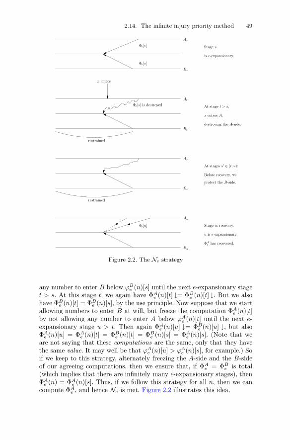
2.14. The infinite injury priority method 49
u is e-expansionary.
x enters
As
Bt
Bs
At stage t > s,
destroying the A-side.
x enters A,
Stage s
is e-expansionary.
restrained
As′
Bs′
Au
Bu
At
Φe[s]
Φe[s]
Φe[s] is destroyed
restrained
At stages s′ ∈ (t, u):
protect the B-side.
Before recovery, we
Φe[u] Stage u: recovery.
ΦAe has recovered.
Figure 2.2. The Ne strategy
any number to enter B below ϕBe (n)[s] until the next e-expansionary staget > s. At this stage t, we again have ΦAe (n)[t] ↓= ΦBe (n)[t] ↓. But we alsohave ΦBe (n)[t] = ΦBe (n)[s], by the use principle. Now suppose that we startallowing numbers to enter B at will, but freeze the computation ΦAe (n)[t]by not allowing any number to enter A below ϕAe (n)[t] until the next e-expansionary stage u > t. Then again ΦAe (n)[u] ↓= ΦBe (n)[u] ↓, but alsoΦAe (n)[u] = ΦAe (n)[t] = ΦBe (n)[t] = ΦBe (n)[s] = ΦAe (n)[s]. (Note that weare not saying that these computations are the same, only that they havethe same value. It may well be that ϕAe (n)[u] > ϕAe (n)[s], for example.) Soif we keep to this strategy, alternately freezing the A-side and the B-sideof our agreeing computations, then we ensure that, if ΦAe = ΦBe is total(which implies that there are infinitely many e-expansionary stages), thenΦAe (n) = ΦAe (n)[s]. Thus, if we follow this strategy for all n, then we cancompute ΦAe , and hence Ne is met. Figure 2.2 illustrates this idea.

50 2. Computability Theory
In summary, the strategy for meeting Ne is to wait until an e-expansionary stage s, then impose a restraint u(e, s) on A, then wait untilthe next e-expansionary stage t, lift the restraint on A, and impose a re-straint u(e, t) on B, and then continue in this way, alternating which set isrestrained at each new e-expansionary stage. Note that there is an impor-tant difference between this strategy and the one employed in the proof ofthe Sacks Splitting Theorem. There we argued that the length of agreementassociated with a given requirement could not go to infinity. Here, however,it may well be the case that lims l(e, s) = ∞, and hence lims u(e, s) = ∞.Thus, the restraints imposed by the strategy for Ne may tend to infinity.
How do the R- and Q-requirements of weaker priority deal with thispossibility? Consider a requirement Ri weaker than Ne. We have twostrategies for Ri. One strategy guesses that there are only finitely manye-expansionary stages. This strategy picks a fresh large follower. Each timea new e-expansionary stage occurs, the strategy is initialized, which meansthat it must pick a new fresh large follower. Otherwise, the strategy actsexactly as described above. That is, it waits until its current follower xenters Wi, if ever, then puts x into A.
The other strategy for Ri guesses that there are infinitely many e-expansionary stages. It picks a follower x. If x enters Wi at stage s, thenit wants to put x into A, but it may be restrained from doing so by thestrategy for Ne. However, if its guess is correct then there will be an e-expansionary stage t � s at which the restraint on A is dropped. At thatstage, x can be put into A.Coherence. When we consider multiple N -requirements, we run into aproblem. Consider two requirements Ne and Ni, with the first havingstronger priority. Let s0 < s1 < · · · be the e-expansionary stages andt0 < t1 < · · · be the i-expansionary stages. During the interval [s0, s1),weaker strategies are prevented from putting certain numbers into A byNe. At stage s1, this restraint is lifted, but if t0 � s1 < t1, then at stages1 it will be Ni that prevents weaker strategies from putting certain num-bers into A. When Ni drops that restraint at stage t1, we may have a newrestraint on A imposed by Ne (if say s2 � t1 < s3). Thus, although indi-vidually Ne and Ni each provide infinitely many stages at which they allowweaker strategies to put numbers into A, the two strategies together mayconspire to block weaker strategies from ever putting numbers into A.
This problem is overcome by having two strategies for Ni. The one guess-ing that there are only finitely many e-expansionary stages has no problems.The one guessing that there are infinitely many e-expansionary stages actsonly at such stages, and in particular calculates its expansionary stagesbased only on such stages, which forces its expansionary stages to be nestedwithin the e-expansionary stages. Thus the actions of Ne and Ni are forcedto cohere.
We now turn to the formal details of the construction. These details mayat first appear somewhat mysterious, in that it may be unclear how they ac-
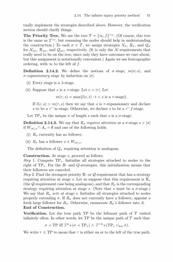
2.14. The infinite injury priority method 51
tually implement the strategies described above. However, the verificationsection should clarify things.The Priority Tree. We use the tree T = {∞, f}<ω. (Of course, this treeis the same as 2<ω, but renaming the nodes should help in understandingthe construction.) To each σ ∈ T , we assign strategies Nσ, Rσ, and Qσfor N|σ|, R|σ|, and Q|σ|, respectively. (It is only the N -requirements thatreally need to be on the tree, since only they have outcomes we care about,but this assignment is notationally convenient.) Again we use lexicographicordering, with ∞ to the left of f .
Definition 2.14.2. We define the notions of σ-stage, m(σ, s), andσ-expansionary stage by induction on |σ|.
(i) Every stage is a λ-stage.
(ii) Suppose that s is a τ -stage. Let e = |τ |. Let
m(τ, s) = max{l(e, t) : t < s is a τ -stage}.
If l(e, s) > m(τ, s) then we say that s is τ -expansionary and declares to be a τ�∞-stage. Otherwise, we declare s to be a τ�f -stage.
Let TPs be the unique σ of length s such that s is a σ-stage.
Definition 2.14.3. We say that Rσ requires attention at a σ-stage s > |σ|if W|σ|,s ∩As = ∅ and one of the following holds.
(i) Rσ currently has no follower.
(ii) Rσ has a follower x ∈W|σ|,s.
The definition of Qσ requiring attention is analogous.
Construction. At stage s, proceed as follows.Step 1. Compute TPs. Initialize all strategies attached to nodes to theright of TPs. For the R- and Q-strategies, this initialization means thattheir followers are canceled.Step 2. Find the strongest priority R- or Q-requirement that has a strategyrequiring attention at stage s. Let us suppose that this requirement is Re
(the Q-requirement case being analogous), and thatRσ is the correspondingstrategy requiring attention at stage s. (Note that s must be a σ-stage.)We say that Rσ acts at stage s. Initialize all strategies attached to nodesproperly extending σ. If Rσ does not currently have a follower, appoint afresh large follower for Rσ. Otherwise, enumerate Rσ’s follower into A.End of Construction.Verification. Let the true path TP be the leftmost path of T visitedinfinitely often. In other words, let TP be the unique path of T such that
σ ≺ TP iff ∃∞s (σ ≺ TPs) ∧ ∃<∞s (TPs <lex σ).
We write τ � TP to mean that τ is either on or to the left of the true path.

52 2. Computability Theory
Lemma 2.14.4. Each R- and Q-requirement is met.
Proof. Consider Re (the Q-requirement case being analogous). Let σ =TP � e. Assume by induction that the strategies attached to proper prefixesof σ act only finitely often, and let s be the least stage such that
1. no strategy attached to a proper prefix of σ acts after stage s and
2. TPt is not to the left of σ for all t > s.
By the minimality of s, it must be the case that Rσ is initialized at stages. Thus, at the next σ-stage t > s, it will be assigned a follower x. SinceRσ cannot be initialized after stage t, this follower is permanent. By theway followers are chosen, x will not be put into A unless x enters We. Ifx enters We at stage u > t, then at the first σ-stage v � u, the strategyRσ will act, and x will enter A. In any case, Rσ succeeds in meeting Re.Note that Rσ acts at most twice after stage s, and hence the induction cancontinue.
Lemma 2.14.5. Each N -requirement is met.
Proof. Consider Ne. Let σ = TP � e. If σ�f ≺ TP then there are onlyfinitely many e-expansionary stages, so Φe(A) �= Φe(B), and hence Ne ismet.
So suppose that σ�∞ ≺ TP and that ΦAe is total. We will show that ΦAeis computable. Let s be the least stage such that
1. no strategy attached to a prefix of σ (including σ itself) acts afterstage s and
2. TPt is not to the left of σ for all t > s.
To compute ΦAe (n), find the least σ�∞-stage t0 > s such that l(e, s) > n.We claim that ΦAe (n) = ΦAe (n)[t0].
Let t0 < t1 < · · · be the σ�∞-stages greater than or equal to t0.Each such stage is e-expansionary, so we have ΦAe (n)[ti] = ΦBe (n)[ti] forall i. We claim that, for each i, we have either ΦAe (n)[ti+1] = ΦAe (n)[ti]or ΦBe (n)[ti+1] = ΦBe (n)[ti]. Assuming this claim, it follows easily thatΦAe (n)[t0] = ΦAe (n)[t1] = · · · , which implies that ΦAe (n) = ΦAe (n)[t0].
To establish the claim, fix i. At stage ti, we initialize all strategies to theright of σ�∞. Thus, any follower of such a strategy appointed after stageti must be larger than any number seen in the construction by stage ti,and in particular larger than ϕAe (n)[ti] and ϕBe (n)[ti]. By the choice of s,strategies above or to the left of σ do not act after stage s. Thus, the onlystrategies that can put numbers less than ϕAe (n)[ti] into A or numbers lessthan ϕBe (n)[ti] into B between stages ti and ti+1 are the ones associatedwith extensions of σ�∞. But such a strategy cannot act except at a σ�∞-stage, and at each stage at most one strategy gets to act. Thus, at most onestrategy associated with an extension of σ�∞ can act between stages ti

2.14. The infinite injury priority method 53
and ti+1, and hence only one of A � ϕAe (n)[ti] and B � ϕBe (n)[ti] can changebetween stages ti and ti+1. So either A � ϕAe (n)[ti+1] = A � ϕAe (n)[ti] orB � ϕBe (n)[ti+1] = B � ϕBe (n)[ti], which implies that either ΦAe (n)[ti+1] =ΦAe (n)[ti] or ΦBe (n)[ti+1] = ΦBe (n)[ti]. As mentioned above, it follows thatΦAe (n) = ΦAe (n)[t0].
These two lemmas show that all requirements are met, which concludesthe proof of the theorem.
Giving a full proof of the following result is a good exercise for thoseunfamiliar with the methodology above.
Theorem 2.14.6 (Ambos-Spies [5], Downey and Welch [135]). There is anoncomputable c.e. set A such that if C �D = A is a c.e. splitting of A,then the degrees of C and D form a minimal pair.
Proof sketch. The proof is similar to that of Theorem 2.14.1, using thelength of agreement function
l(i, j, k,m, s) = max{x : ∀y < x [ΦWki (y)[s]↓= ΦWm
j (y)[s]↓∧ ∀z � ϕWk
i (y)[s], ϕWm
j (y)[s] (Wk[s] � z �Wm[s] � z = As � z)]}.
2.14.3 High computably enumerable degrees
Another example of an infinite injury argument is the construction of anincomplete high c.e. degree. Recall that a c.e. degree a is high if a′ = 0′′.We begin with a few definitions. Recall that A[e] denotes the eth column{〈e, n〉 : 〈e, n〉 ∈ A} of A.
Definition 2.14.7. A set A is piecewise trivial if for all e, the set A[e] iseither finite or equal to N[e].
A subset B of A is thick if for all e we have A[e] =∗ B[e] (i.e., thesymmetric difference of A[e] and B[e] is finite).
Lemma 2.14.8. (i) There is a piecewise trivial c.e. set A such that A[e]
is infinite iff Φe is total.
(ii) If B is a thick subset of such a set A, then B is high.
Proof. (i) Let A = {〈e, n〉 : e ∈ N ∧ ∀k � nΦe(k) ↓}. Then A is c.e., andclearly A[e] is infinite iff A[e] = N[e] iff Φe is total.
(ii) Define a reduction Γ by letting ΓX(e, s) = 1 if 〈e, s〉 ∈ X andΓX(e, s) = 0 otherwise. If Φe is total then A[e] = N[e], so B[e] is coinfi-nite, which implies that lims ΓB(e, s) = 1. On the other hand, if Φe is nottotal then A[e] is finite, so B[e] is finite, which implies that lims ΓB(e, s) = 0.

54 2. Computability Theory
Thus, the function f defined by f(e) = lims ΓB(e, s) is total. By the rela-tivized form of the limit lemma, f �T B
′. So B′ can decide whether a givenΦe is total or not. By Theorem 2.6.5, ∅′′ �T B
′.
Thus, to construct an incomplete high c.e. degree, it suffices to prove thefollowing result, which is a weak form of the Thickness Lemma discussedin the next section.
Theorem 2.14.9 (Shoenfield [355]). Let C be a noncomputable c.e. set,and let A be a piecewise trivial c.e. set. Then there is a c.e. thick subset Bof A such that C �T B.
Proof. We construct B ⊆ A to meet the following requirements for all e.
Re : |A[e] \B[e]| <∞.
Ne : ΦBe �= C.
We give the intuition and formal details of the construction, and sketch outits verification, leaving some details to the reader.
To meet Re, we must make sure that almost all of the eth column of Agets into B. To meet Ne, we use the strategy already employed in the proofof the Sacks Splitting Theorem 2.12.1. That is, we measure the length ofagreement
l(e, s) = max{n : ∀k < n (ΦBe (k)[s] = Cs(k))},
with the idea of preserving Bs on the use ϕBe (n)[s] for all n < l(e, s).The problem comes from the interaction of this preservation strategy
with the strategies for stronger priority R-requirements, since these maybe infinitary. It might be the case that we infinitely often try to preserve anagreeing computation ΦBe (n)[s] = Cs(n), only to have some 〈i, x〉 enter Awith i < e and 〈i, x〉 < ϕBe (n)[s]. Since we must put almost every such pairinto B to meet Ri, our strategy for meeting Ne might be injured infinitelyoften.
On the other hand, we do know that Ri can do only one of two things.Either A[i] is finite, and hence Ri stops injuring Ne after some time, oralmost all of A[i] is put into B. In the latter case, the numbers put intoB for the sake of Ri form a computable set (since A is piecewise trivial).It is easy to adapt the strategy for Ne to deal with this case. Let S bethe computable set of numbers put into B for the sake of Ri. We canthen proceed with the Sacks preservation strategy, except that we do notbelieve a computation ΦBe (k)[s] unless Bs already contains every elementof S � ϕBe (k)[s]. This modification prevents the action taken for Ri fromever injuring the strategy for meeting Ne.
Of course, we do not know which of the two possibilities for the action ofRi actually happens, so, as before, we will have multiple strategies for Ne,representing guesses as to whether or not A[i] is finite. There are several
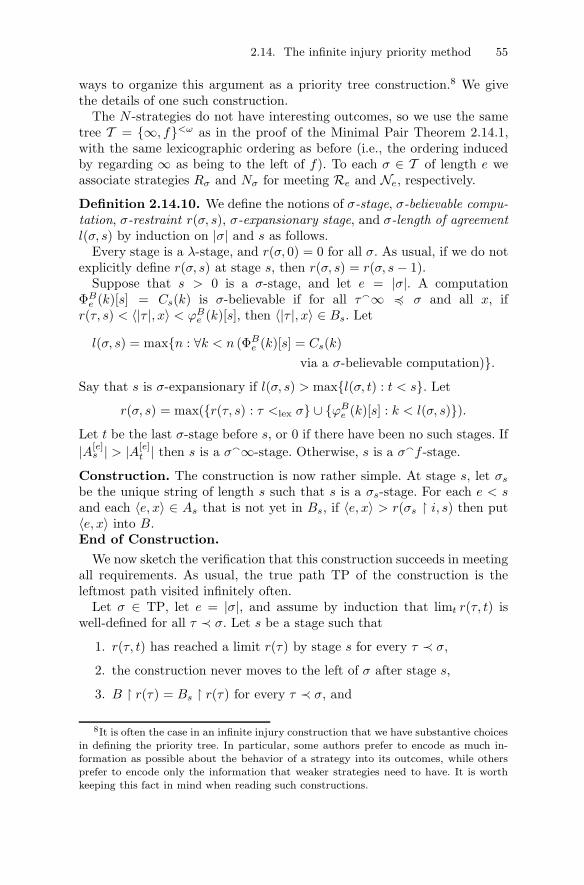
2.14. The infinite injury priority method 55
ways to organize this argument as a priority tree construction.8 We givethe details of one such construction.
The N -strategies do not have interesting outcomes, so we use the sametree T = {∞, f}<ω as in the proof of the Minimal Pair Theorem 2.14.1,with the same lexicographic ordering as before (i.e., the ordering inducedby regarding ∞ as being to the left of f). To each σ ∈ T of length e weassociate strategies Rσ and Nσ for meeting Re and Ne, respectively.
Definition 2.14.10. We define the notions of σ-stage, σ-believable compu-tation, σ-restraint r(σ, s), σ-expansionary stage, and σ-length of agreementl(σ, s) by induction on |σ| and s as follows.
Every stage is a λ-stage, and r(σ, 0) = 0 for all σ. As usual, if we do notexplicitly define r(σ, s) at stage s, then r(σ, s) = r(σ, s − 1).
Suppose that s > 0 is a σ-stage, and let e = |σ|. A computationΦBe (k)[s] = Cs(k) is σ-believable if for all τ�∞ � σ and all x, ifr(τ, s) < 〈|τ |, x〉 < ϕBe (k)[s], then 〈|τ |, x〉 ∈ Bs. Let
l(σ, s) = max{n : ∀k < n (ΦBe (k)[s] = Cs(k)via a σ-believable computation)}.
Say that s is σ-expansionary if l(σ, s) > max{l(σ, t) : t < s}. Let
r(σ, s) = max({r(τ, s) : τ <lex σ} ∪ {ϕBe (k)[s] : k < l(σ, s)}).Let t be the last σ-stage before s, or 0 if there have been no such stages. If|A[e]s | > |A[e]
t | then s is a σ�∞-stage. Otherwise, s is a σ�f -stage.
Construction. The construction is now rather simple. At stage s, let σsbe the unique string of length s such that s is a σs-stage. For each e < sand each 〈e, x〉 ∈ As that is not yet in Bs, if 〈e, x〉 > r(σs � i, s) then put〈e, x〉 into B.End of Construction.
We now sketch the verification that this construction succeeds in meetingall requirements. As usual, the true path TP of the construction is theleftmost path visited infinitely often.
Let σ ∈ TP, let e = |σ|, and assume by induction that limt r(τ, t) iswell-defined for all τ ≺ σ. Let s be a stage such that
1. r(τ, t) has reached a limit r(τ) by stage s for every τ ≺ σ,
2. the construction never moves to the left of σ after stage s,
3. B � r(τ) = Bs � r(τ) for every τ ≺ σ, and
8It is often the case in an infinite injury construction that we have substantive choicesin defining the priority tree. In particular, some authors prefer to encode as much in-formation as possible about the behavior of a strategy into its outcomes, while othersprefer to encode only the information that weaker strategies need to have. It is worthkeeping this fact in mind when reading such constructions.
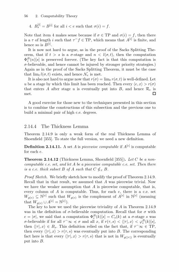
56 2. Computability Theory
4. B[i]s = B[i] for all i < e such that σ(i) = f .
Note that item 4 makes sense because if σ ∈ TP and σ(i) = f , then thereis a τ of length i such that τ�f ∈ TP, which means that A[i] is finite, andhence so is B[i].
It is now not hard to argue, as in the proof of the Sacks Splitting The-orem, that if t > s is a σ-stage and n < l(σ, t), then the computationΦBe (n)[s] is preserved forever. (The key fact is that this computation isσ-believable, and hence cannot be injured by stronger priority strategies.)Again as in the proof of the Sacks Splitting Theorem, it must be the casethat limt l(σ, t) exists, and hence Ne is met.
It is also not hard to argue now that r(σ) = limt r(σ, t) is well-defined. Letu be a stage by which this limit has been reached. Then every 〈e, x〉 > r(σ)that enters A after stage u is eventually put into B, and hence Re ismet.
A good exercise for those new to the techniques presented in this sectionis to combine the constructions of this subsection and the previous one tobuild a minimal pair of high c.e. degrees.
2.14.4 The Thickness Lemma
Theorem 2.14.9 is only a weak form of the real Thickness Lemma ofShoenfield [355]. To state the full version, we need a new definition.
Definition 2.14.11. A set A is piecewise computable if A[e] is computablefor each e.
Theorem 2.14.12 (Thickness Lemma, Shoenfield [355]). Let C be a non-computable c.e. set, and let A be a piecewise computable c.e. set. Then thereis a c.e. thick subset B of A such that C �T B.
Proof Sketch. We briefly sketch how to modify the proof of Theorem 2.14.9.Recall that in that result, we assumed that A was piecewise trivial. Nowwe have the weaker assumption that A is piecewise computable, that is,every column of A is computable. Thus, for each e, there is a c.e. setWg(e) ⊆ N[e] such that Wg(e) is the complement of A[e] in N[e] (meaningthat Wg(e) �A[e] = N[e]).
The key to how we used the piecewise triviality of A in Theorem 2.14.9was in the definition of σ-believable computation. Recall that for σ withe = |σ|, we said that a computation ΦBe (k)[s] = Cs(k) at a σ-stage s wasσ-believable if for all τ�∞ � σ and all x, if r(τ, s) < 〈|τ |, x〉 < ϕBe (k)[s],then 〈|τ |, x〉 ∈ Bs. This definition relied on the fact that, if τ�∞ ∈ TP,then every 〈|τ |, x〉 > r(τ, s) was eventually put into B. The correspondingfact here is that every 〈|τ |, x〉 > r(τ, s) that is not in Wg(|τ |) is eventuallyput into B.

2.14. The infinite injury priority method 57
So in order to adjust the definition of σ-believable computation, for eachτ ≺ σ, we need to know an index j such that Wj = Wg(|τ |). Since we cannotcompute such a j from |τ |, we must guess it along the tree of strategies.That is, for each τ , instead of the outcomes ∞ and f , we now have anoutcome j for each j ∈ N, representing a guess that Wj = Wg(|τ |). Theoutcome j is taken to be correct at a stage s if j is the least number forwhich we see the length of agreement between N[e] and A[e] �Wj increaseat stage s.
Now a computation ΦBe (k)[s] = Cs(k) at a σ-stage s is σ-believable if forall τ�j � σ and all x, if r(τ, s) < 〈|τ |, x〉 < ϕBe (k)[s], then 〈|τ |, x〉 ∈ Bs∪Wj .The rest of the construction is essentially the same as before. One importantpoint is that, because the tree of strategies is now infinitely branching, theexistence of the true path is no longer automatically guaranteed. However,if τ is visited infinitely often then τ�j is visited infinitely often for theleast j such that Wj = Wg(|τ |), from which it follows that TP is well-defined. There are infinite injury constructions in which showing that TPis well-defined requires a careful proof.
We make some remarks for those who, like the senior author, werebrought up with the “old” techniques using the “hat trick” and the “win-dow lemma” of Soare [366]. It is rather ironic that the very first result thatused the infinite injury method in its proof was the Thickness Lemma,since, like the Density Theorem of the next section, it has a proof not us-ing priority trees that is combinatorially much easier to present. In a sense,this fact shows an inherent shortcoming of the tree technique in that oftenmore information needs to be represented on the tree than is absolutelynecessary for the proof of the theorem. To demonstrate this point, andsince it is somewhat instructive, we now sketch the original proof of theThickness Lemma.
We have the same requirements, but we define ΦB(n)[s] to be ΦB(n)[s]unless some number less than ϕB(n)[s] enters B at stage s, in which casewe declare that ΦB(n)[s] ↑. This is called the hat convention. Using thisconvention, we can generate the hatted length of agreement l(e, s) with Φin place of Φ, and so forth. Finally, we define the restraint function
r(e, s) = max{ϕB(n)[s] : n < l(e, s)}.
The construction is to put 〈e, x〉 ∈ As into B at stage s if it is not yetthere and 〈e, x〉 > max{r(j, s) : j � e}.
To verify that this construction succeeds in meeting all our requirements,it is enough to show that, for each e, the injury set
Ie,s = {x : ∃v � s (x � r(e, v) ∧ x ∈ Bs+1 \Bv)}
is computable, B[e] =∗ A[e], and Ne is met, all by simultaneous induction,the key idea being the “window lemma”, which states that the liminf ofthe restraint R(e, s) = max{r(j, s) : j � e} is finite. The key point is
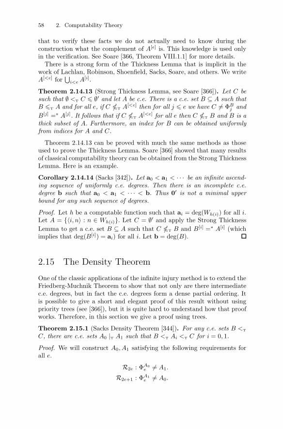
58 2. Computability Theory
that to verify these facts we do not actually need to know during theconstruction what the complement of A[e] is. This knowledge is used onlyin the verification. See Soare [366, Theorem VIII.1.1] for more details.
There is a strong form of the Thickness Lemma that is implicit in thework of Lachlan, Robinson, Shoenfield, Sacks, Soare, and others. We writeA[<e] for
⋃i<eA
[i].
Theorem 2.14.13 (Strong Thickness Lemma, see Soare [366]). Let C besuch that ∅ <T C � ∅′ and let A be c.e. There is a c.e. set B ⊆ A such thatB �T A and for all e, if C �T A
[<e] then for all j � e we have C �= ΦBj andB[j] =∗ A[j]. It follows that if C �T A
[<e] for all e then C �T B and B is athick subset of A. Furthermore, an index for B can be obtained uniformlyfrom indices for A and C.
Theorem 2.14.13 can be proved with much the same methods as thoseused to prove the Thickness Lemma. Soare [366] showed that many resultsof classical computability theory can be obtained from the Strong ThicknessLemma. Here is an example.
Corollary 2.14.14 (Sacks [342]). Let a0 < a1 < · · · be an infinite ascend-ing sequence of uniformly c.e. degrees. Then there is an incomplete c.e.degree b such that a0 < a1 < · · · < b. Thus 0′ is not a minimal upperbound for any such sequence of degrees.
Proof. Let h be a computable function such that ai = deg(Wh(i)) for all i.Let A = {〈i, n〉 : n ∈ Wh(i)}. Let C = ∅′ and apply the Strong ThicknessLemma to get a c.e. set B ⊆ A such that C �T B and B[i] =∗ A[i] (whichimplies that deg(B[i]) = ai) for all i. Let b = deg(B).
2.15 The Density Theorem
One of the classic applications of the infinite injury method is to extend theFriedberg-Muchnik Theorem to show that not only are there intermediatec.e. degrees, but in fact the c.e. degrees form a dense partial ordering. Itis possible to give a short and elegant proof of this result without usingpriority trees (see [366]), but it is quite hard to understand how that proofworks. Therefore, in this section we give a proof using trees.
Theorem 2.15.1 (Sacks Density Theorem [344]). For any c.e. sets B <T
C, there are c.e. sets A0 |T A1 such that B <T Ai <T C for i = 0, 1.
Proof. We will construct A0, A1 satisfying the following requirements forall e.
R2e : ΦA0e �= A1.
R2e+1 : ΦA1e �= A0.
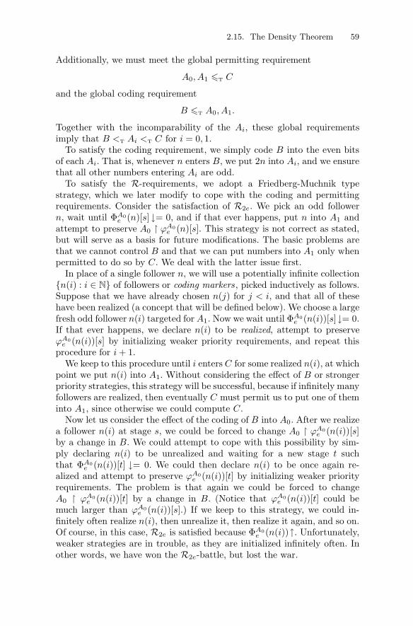
2.15. The Density Theorem 59
Additionally, we must meet the global permitting requirement
A0, A1 �T C
and the global coding requirement
B �T A0, A1.
Together with the incomparability of the Ai, these global requirementsimply that B <T Ai <T C for i = 0, 1.
To satisfy the coding requirement, we simply code B into the even bitsof each Ai. That is, whenever n enters B, we put 2n into Ai, and we ensurethat all other numbers entering Ai are odd.
To satisfy the R-requirements, we adopt a Friedberg-Muchnik typestrategy, which we later modify to cope with the coding and permittingrequirements. Consider the satisfaction of R2e. We pick an odd followern, wait until ΦA0
e (n)[s] ↓= 0, and if that ever happens, put n into A1 andattempt to preserve A0 � ϕA0
e (n)[s]. This strategy is not correct as stated,but will serve as a basis for future modifications. The basic problems arethat we cannot control B and that we can put numbers into A1 only whenpermitted to do so by C. We deal with the latter issue first.
In place of a single follower n, we will use a potentially infinite collection{n(i) : i ∈ N} of followers or coding markers , picked inductively as follows.Suppose that we have already chosen n(j) for j < i, and that all of thesehave been realized (a concept that will be defined below). We choose a largefresh odd follower n(i) targeted forA1. Now we wait until ΦA0
e (n(i))[s]↓= 0.If that ever happens, we declare n(i) to be realized, attempt to preserveϕA0e (n(i))[s] by initializing weaker priority requirements, and repeat this
procedure for i+ 1.We keep to this procedure until i enters C for some realized n(i), at which
point we put n(i) into A1. Without considering the effect of B or strongerpriority strategies, this strategy will be successful, because if infinitely manyfollowers are realized, then eventually C must permit us to put one of theminto A1, since otherwise we could compute C.
Now let us consider the effect of the coding of B into A0. After we realizea follower n(i) at stage s, we could be forced to change A0 � ϕA0
e (n(i))[s]by a change in B. We could attempt to cope with this possibility by sim-ply declaring n(i) to be unrealized and waiting for a new stage t suchthat ΦA0
e (n(i))[t] ↓= 0. We could then declare n(i) to be once again re-alized and attempt to preserve ϕA0
e (n(i))[t] by initializing weaker priorityrequirements. The problem is that again we could be forced to changeA0 � ϕA0
e (n(i))[t] by a change in B. (Notice that ϕA0e (n(i))[t] could be
much larger than ϕA0e (n(i))[s].) If we keep to this strategy, we could in-
finitely often realize n(i), then unrealize it, then realize it again, and so on.Of course, in this case, R2e is satisfied because ΦA0
e (n(i))↑. Unfortunately,weaker strategies are in trouble, as they are initialized infinitely often. Inother words, we have won the R2e-battle, but lost the war.

60 2. Computability Theory
The solution to this dilemma is to notice that this ugly situation canhappen only if the values of ϕA0
e (n(i))[s] are unbounded for some i. If weknew this to be the case, then we could do the construction ignoring R2e,as it would automatically be satisfied. Obviously, though, we cannot knowwhether this situation happens ahead of time. However, we can have aninfinitary outcome for R2e, which guesses that this use is unbounded. Thetrick is to make the effect on the construction of this outcome computable,hence allowing strategies below it to live with the action of R2e if it trulyhas this infinitary outcome.
To make this idea more precise, we begin by presenting the basic modulefor the R2e strategy described above, in the absence of stronger priorityrequirements. (Thus the single strategy for R0, the strongest requirement,acts exactly as follows.) The basic module for R2e+1 strategies is of coursesymmetric.
1. If all currently defined followers are realized, then choose a large freshodd follower n(i).
2. If ΦA0e (n(i))[s] ↓= 0, then declare n(i) to be realized and initialize
weaker strategies.
3. If n(i) is realized and i enters C, then put n(i) into A1. In this case,stop choosing new followers unless n(i) later becomes unrealized.
4. If n(i) is realized and the coding of B causes A0 to change belowϕA0e (n(i))[t] at stage t, then, for the least i for which this is the case
at this stage, cancel all n(j) for j > i (which will have different valuesif defined again later) and declare n(i) to be unrealized.
Note that at each stage s, the strategy for R2e has realized followersn(0), . . . , n(i−1) and an unrealized follower n(i). For each realized followern(j), we have ΦA0
e (n(j))[s]↓.To see that the above module succeeds in satisfying a single requirement
R2e, suppose not, so that ΦA0e = A1. Then each n(i) is eventually defined
and reaches a final value, since all uses of the form ϕA0e (n(i)) eventually
settle. Moreover, we can compute these final values using B, since it isonly the coding of B into A0 that can change these uses. Now we claimthat B can compute C, contrary to hypothesis. Given i, we can use Bto compute a stage s at which n(i) reaches its final value and becomespermanently realized. If i were to enter C after stage s, then n(i) wouldenter A1, ensuring that ΦA0
e �= A1. Thus i ∈ C iff i ∈ Cs.The above also shows that this module has two possible kinds of out-
comes. Either ϕA0e (n(i)) is unbounded for some i, or ΦA0
e (n(i)) �= A1(n(i)).We denote the former outcome by (i, u) and the latter by (i, f). We usethese outcomes to generate the priority tree T = {(i, u), (i, f) : i ∈ N}<ω,with a lexicographic ordering inherited from the ordering of outcomes(i, u) <L (i, f) <L (i+ 1, u).

2.15. The Density Theorem 61
We now discuss how weaker priority requirements can live in the environ-ments provided by R2e, by considering the case e = 0. The markers n(i) forthe R0 strategy will now be denoted by n(λ, i) (since that strategy is asso-ciated with the empty sequence in T ). There are infinitely many strategiesfor R1, one for each outcome. We denote the strategy below outcome σ byRσ and its markers by n(σ, i).
A strategy living below (i, f) guesses that the strategy for R0 has finiteaction. Hence it can be initialized each time we realize n(λ, j) for j � i,and simply implements the basic module.
A strategy Rσ living below σ = (i, u) guesses that n(λ, i) comes to afinal value but no n(λ, j) for j > i does, because we keep changing A0
below ϕA00 (n(λ, i))[s] for the sake of coding B. As in the Thickness Lemma,
this strategy will believe a ΦA10 -computation only if the current value of
n(λ, i + 1) (and hence every n(λ, j) for j > i) is greater than the use ofthat computation.
However, there is a problem here. The strategy Rσ may want to put num-bers into A0 smaller than uses that the R0 strategy is trying to preserve.For instance, say a follower n(σ, j) is appointed, then followers n(λ, k) withk > i are appointed and become realized with corresponding uses largerthan n(σ, j), then n(σ, j) becomes realized and permitted by C. If the guessthat (i, u) is the true outcome of the R0 strategy is correct, then there isno problem. We can put n(σ, j) into A0 and still satisfy R0. But otherwise,we cannot afford to allow the enumeration of n(σ, j) to injure R0.
We now come to the main idea of this proof, Sacks’ notion of delayedpermitting: Since Rσ is guessing that (i, u) is the true outcome of the R0
strategy, it believes that any use larger than n(σ, j) that the R0 strategy istrying to preserve will eventually be violated by the coding of B into A0.So once n(σ, j) is realized and C-permitted, instead of immediately puttingn(σ, j) into A0, we merely promise to put it there if these uses do go away;that is, if Rσ becomes accessible again before n(σ, j) is initialized.
This delayed permitting still allows C to compute A0, because C cancompute B, and hence know whether the relevant uses will ever be violated.That is, given a realized follower n(σ, j), the set C knows whether j ∈ C.If not, then n(σ, j) never enters A0. Otherwise, C can check what theB-conditions are for Rσ to be accessible again, find out whether theseconditions will ever obtain, and if so, go to that stage of the constructionto check whether n(σ, j) has not been initialized in the meantime, which isthe only case in which n(σ, j) enters A0.
It is a subtle fact that, while the true path of the construction remainscomputable only from 0′′, the fate of a particular follower is always com-putable from C. Furthermore, we can still argue that, if σ = (i, u) is in factthe true outcome of R0 strategy and Rσ fails, then B can compute C, inmuch the same way as before, since every C-permitted follower eventuallyhas no restraint placed on it.
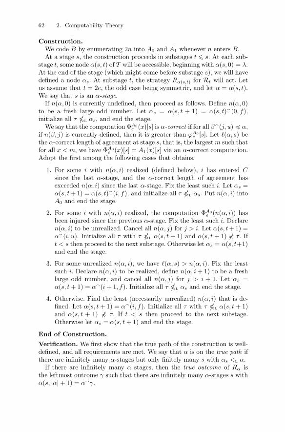
62 2. Computability Theory
Construction.We code B by enumerating 2n into A0 and A1 whenever n enters B.At a stage s, the construction proceeds in substages t � s. At each sub-
stage t, some node α(s, t) of T will be accessible, beginning with α(s, 0) = λ.At the end of the stage (which might come before substage s), we will havedefined a node αs. At substage t, the strategy Rα(s,t) for Rt will act. Letus assume that t = 2e, the odd case being symmetric, and let α = α(s, t).We say that s is an α-stage.
If n(α, 0) is currently undefined, then proceed as follows. Define n(α, 0)to be a fresh large odd number. Let αs = α(s, t + 1) = α(s, t)�(0, f),initialize all τ �L αs, and end the stage.
We say that the computation ΦA0e (x)[s] is α-correct if for all β�(j, u) � α,
if n(β, j) is currently defined, then it is greater than ϕA0e [s]. Let (α, s) be
the α-correct length of agreement at stage s, that is, the largestm such thatfor all x < m, we have ΦA0
e (x)[s] = A1(x)[s] via an α-correct computation.Adopt the first among the following cases that obtains.
1. For some i with n(α, i) realized (defined below), i has entered Csince the last α-stage, and the α-correct length of agreement hasexceeded n(α, i) since the last α-stage. Fix the least such i. Let αs =α(s, t+ 1) = α(s, t)�(i, f), and initialize all τ �L αs. Put n(α, i) intoA0 and end the stage.
2. For some i with n(α, i) realized, the computation ΦA0e (n(α, i)) has
been injured since the previous α-stage. Fix the least such i. Declaren(α, i) to be unrealized. Cancel all n(α, j) for j > i. Let α(s, t+1) =α�(i, u). Initialize all τ with τ �L α(s, t + 1) and α(s, t + 1) �� τ . Ift < s then proceed to the next substage. Otherwise let αs = α(s, t+1)and end the stage.
3. For some unrealized n(α, i), we have (α, s) > n(α, i). Fix the leastsuch i. Declare n(α, i) to be realized, define n(α, i+ 1) to be a freshlarge odd number, and cancel all n(α, j) for j > i + 1. Let αs =α(s, t+ 1) = α�(i+ 1, f). Initialize all τ �L αs and end the stage.
4. Otherwise. Find the least (necessarily unrealized) n(α, i) that is de-fined. Let α(s, t+ 1) = α�(i, f). Initialize all τ with τ �L α(s, t + 1)and α(s, t + 1) �� τ . If t < s then proceed to the next substage.Otherwise let αs = α(s, t+ 1) and end the stage.
End of Construction.
Verification. We first show that the true path of the construction is well-defined, and all requirements are met. We say that α is on the true path ifthere are infinitely many α-stages but only finitely many s with αs <L α.
If there are infinitely many α stages, then the true outcome of Rα isthe leftmost outcome γ such that there are infinitely many α-stages s withα(s, |α| + 1) = α�γ.

2.15. The Density Theorem 63
Lemma 2.15.2. Let α be on the true path, and let γ be its true outcome.Then Rα succeeds in meeting R|α|, there are infinitely many α-stages wherethe stage does not end at substage |α|, and Rα initializes strategies belowα�γ only finitely often.
Proof. Assume by induction that the lemma holds for strategies above α.Then, since α can be initialized only when αs <L α or when a strategyabove it initializes it, there is a stage s0 such that α is not initialized afterstage s0. After this stage, no n(α, i) is canceled except for the sake of ann(α, j) with j < i. Now we can argue as in the basic module, but usingα-correct computations at α-stages, to show that Rα succeeds in meetingR|α|.
If γ = (i, u) then Rα does not initialize strategies below α�γ, and atevery stage s > |α| at which α(s, |α|+ 1) = α�γ, the stage does not end atsubstage |α|.
If γ = (i, f), then the Rα-module acts only finitely often.
Thus, by induction, for each e there is an α of length e such that thereare infinitely many α-stages but only finitely many s with αs <L α, whenceRe is met.
Lemma 2.15.3. A0, A1 �T C.
Proof. We do the A0 case, the Ai case being symmetric.If n ∈ A0, then n must be chosen by stage n as n(α, i) for some α and i
with |α| even and i ∈ C. If that is the case, let s be the stage at which ienters C. Then n will be in A0 iff there is an α-stage t � s at which n(α, i)is still equal to n. So we may assume that s is not itself an α-stage andn(α, i) is not canceled at stage s, since otherwise we would already knowwhether n ∈ A0 at stage s. Thus α <L αs. Let β be the longest commoninitial segment of α and αs. We have two cases.
First suppose that β�(k, f) � α for some k. Then β�(j, o) � αs for somej > k and o ∈ {f, u}. Suppose there is a least β�(k, f)-stage t > s. If theconstruction moves to the left of β�(k, f) between stages s and t then αis initialized, so n /∈ A0. Otherwise, either case 1 or case 3 above holds forβ at stage t, so again α is initialized and n /∈ A0. Of course, if there isno β�(k, f)-stage after s, then n /∈ Ao. Thus, in this case, we know thatn /∈ A0 no matter what happens after stage s.
Now suppose that β�(k, u) � α for some k. After stage s, there can bean α-stage only if there is a β�(k, u)-stage. Now C can use B to figure outwhether the use of the relevant computation ΦAi
e (n(β, k)) is B-correct. Ifit is B-correct, then n /∈ A0, since the only way for there to be a furtherβ�(k, u)-stage is for a strategy above or to the left of β�(k, u) to enumeratesomething into Ai, which causes α to be initialized. If not, then go to a staget where B changes below this use. If t is not a β�(k, u)-stage and n(α, i) isnot canceled at stage t, then αt <L β. Let β′ be the longest common initial

64 2. Computability Theory
segment of β and αt. We can now repeat the above argument with β′ inplace of β.
It is a straightforward exercise to show that, proceeding in this manner,we eventually reach a stage at which we either can be sure that n /∈ A0,or we have an α-stage, at which point n enters A0. Since we do so using Band B �T C, we have A0 �T C.
The two lemmas above complete the proof of the theorem.
2.16 Jump theorems
We will see that the jump operator plays an important role in the study ofalgorithmic randomness. In this section, we look at several classic resultsabout the range of the jump operator, whose proofs are combinations oftechniques we have already seen. Of course, if d = a′ then d � 0′. Thefollowing result is a converse to this fact.
Theorem 2.16.1 (Friedberg Completeness Criterion [160]). If d � 0′ thenthere is a degree a such that a′ = a ∨ 0′ = d.
Proof. This is a finite extension argument. Let D ∈ d. We construct a setA in stages, and let a = deg(A). At stage 0, let A0 = λ.
At odd stages s = 2e+1, we force the jump (i.e., decide whether e ∈ A′).We ask ∅′ whether there is a σ � As−1 such that Φσe (e)↓. If so, we searchfor such a σ and let As = σ. If not, we let As = As−1. Note that, in thiscase, we have ensured that ΦAe (e)↑.
At even stages s = 2e+2, we codeD(e) into A by letting As = As−1D(e).This concludes the construction. We have A⊕∅′ �T A
′ (which is alwaysthe case for any set A), so we can complete the proof by showing thatA′ �T D and D �T A⊕ ∅′.
Since ∅′ �T D, we can carry out the construction computably in D. Todecide whether e ∈ A′, we simply run the construction until stage 2e+ 1.At this stage, we decide whether e ∈ A′. Thus A′ �T D.
A ∅′ oracle can tell us how to obtain A2e+1 given A2e, while an A oraclecan tell us how to obtain A2e+2 given A2e+1, so using A ⊕ ∅′, we cancompute A2n+2 for any given n. Since D(n) is the last element of A2n+2,we can compute D(n) using A⊕ ∅′. Thus D �T A⊕ ∅′.
The above proof should be viewed as a combination of a coding argu-ment and the construction of a low set, done simultaneously. This kind ofcombination is a recurrent theme in the proofs of results such as the onesin this section.
The following extension of the above result is due to Posner and Robinson[315]. We give a proof due to Jockusch and Shore [194].

2.16. Jump theorems 65
Theorem 2.16.2 (Posner and Robinson [315]). r If c > 0 and d � 0′ ∨ cthen there is a degree a such that a′ = a ∨ c = d.
Proof. By Proposition 2.13.1, there is an immune C ∈ c. (Recall that thecomplement of a simple set is immune.) Let D ∈ d. We build a set A byfinite extensions.
Let A0 = λ. Given An, proceed as follows. Let Sn = {x : ∃σ �An0x1 (Φσn(n) ↓)}. If Sn is finite then there is an x ∈ C \ Sn. In thiscase, let An+1 = An0x1D(n). If Sn is infinite then, since Sn is c.e. and Cis immune, there is an x ∈ Sn \ C. In this case, let s be least such that∃σ � An0x1 (Φσn(n)[s] ↓), let σ be the length-lexicographically least stringwitnessing this existential, and let An+1 = σD(n).
It is easy to see that from the sequence A0, A1, . . . we can compute theset A′, the set A⊕ C, and the set D. Thus, it is enough to show that thissequence can be computed from each of these three sets. Suppose we havecomputed An.
Since D �T ∅′ ⊕ C, using D we can compute Sn and C and hencedetermine An+1.
If we have A′, then we have A, so we can determine the x such thatAn0x1 ≺ A. Then using ∅′ we can determine whether x ∈ Sn, and hencedetermine An+1.
If we haveA⊕C, then again we can determine the x such thatAn0x1 ≺ A.By construction, x ∈ Sn iff x /∈ C, so we can then use C to determineAn+1.
It is not hard to show that if A �T ∅′ then A′ is c.e. in ∅′. Since also ∅′ �T
A′, we say that A′ is computably enumerable in and above ∅′, abbreviatedby CEA(∅′). The following theorem is an elaboration of Theorem 2.16.1.
Theorem 2.16.3 (Shoenfield Jump Inversion Theorem [354]). If D isCEA(∅′) then there is an A �T ∅′ such that A′ ≡T D.
We will briefly sketch a proof of the following stronger result. (We restrictourselves to a sketch because, from a modern viewpoint, the proof containsno new ideas beyond what we have seen so far. See Soare [366] for a fullproof.)
Theorem 2.16.4 (Sacks Jump Inversion Theorem [341]). If D is CEA(∅′)then there is a c.e. set A such that A′ ≡T D.
Proof sketch. Let D be CEA(∅′). Then D is Σ02, so there is an approxima-
tion {Ds}s∈ω such that n ∈ D iff there is an s such that n ∈ Dt for allt > s. Arguing as in the proof of Lemma 2.14.8, we have a c.e. set B suchthat B[e] is an initial segment of N[e] and equals N[e] iff e /∈ D.
We need to make the jump of A high enough to compute D, which wedo by meeting for each e the requirement
Pe : A[e] =∗ B[e].
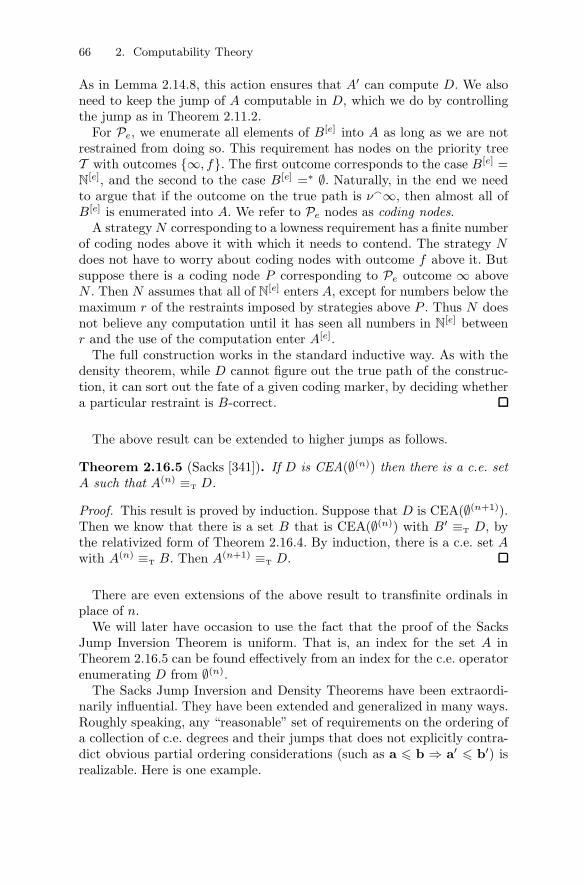
66 2. Computability Theory
As in Lemma 2.14.8, this action ensures that A′ can compute D. We alsoneed to keep the jump of A computable in D, which we do by controllingthe jump as in Theorem 2.11.2.
For Pe, we enumerate all elements of B[e] into A as long as we are notrestrained from doing so. This requirement has nodes on the priority treeT with outcomes {∞, f}. The first outcome corresponds to the case B[e] =N[e], and the second to the case B[e] =∗ ∅. Naturally, in the end we needto argue that if the outcome on the true path is ν�∞, then almost all ofB[e] is enumerated into A. We refer to Pe nodes as coding nodes.
A strategyN corresponding to a lowness requirement has a finite numberof coding nodes above it with which it needs to contend. The strategy Ndoes not have to worry about coding nodes with outcome f above it. Butsuppose there is a coding node P corresponding to Pe outcome ∞ aboveN . Then N assumes that all of N[e] enters A, except for numbers below themaximum r of the restraints imposed by strategies above P . Thus N doesnot believe any computation until it has seen all numbers in N[e] betweenr and the use of the computation enter A[e].
The full construction works in the standard inductive way. As with thedensity theorem, while D cannot figure out the true path of the construc-tion, it can sort out the fate of a given coding marker, by deciding whethera particular restraint is B-correct.
The above result can be extended to higher jumps as follows.
Theorem 2.16.5 (Sacks [341]). If D is CEA(∅(n)) then there is a c.e. setA such that A(n) ≡T D.
Proof. This result is proved by induction. Suppose that D is CEA(∅(n+1)).Then we know that there is a set B that is CEA(∅(n)) with B′ ≡T D, bythe relativized form of Theorem 2.16.4. By induction, there is a c.e. set Awith A(n) ≡T B. Then A(n+1) ≡T D.
There are even extensions of the above result to transfinite ordinals inplace of n.
We will later have occasion to use the fact that the proof of the SacksJump Inversion Theorem is uniform. That is, an index for the set A inTheorem 2.16.5 can be found effectively from an index for the c.e. operatorenumerating D from ∅(n).
The Sacks Jump Inversion and Density Theorems have been extraordi-narily influential. They have been extended and generalized in many ways.Roughly speaking, any “reasonable” set of requirements on the ordering ofa collection of c.e. degrees and their jumps that does not explicitly contra-dict obvious partial ordering considerations (such as a � b ⇒ a′ � b′) isrealizable. Here is one example.
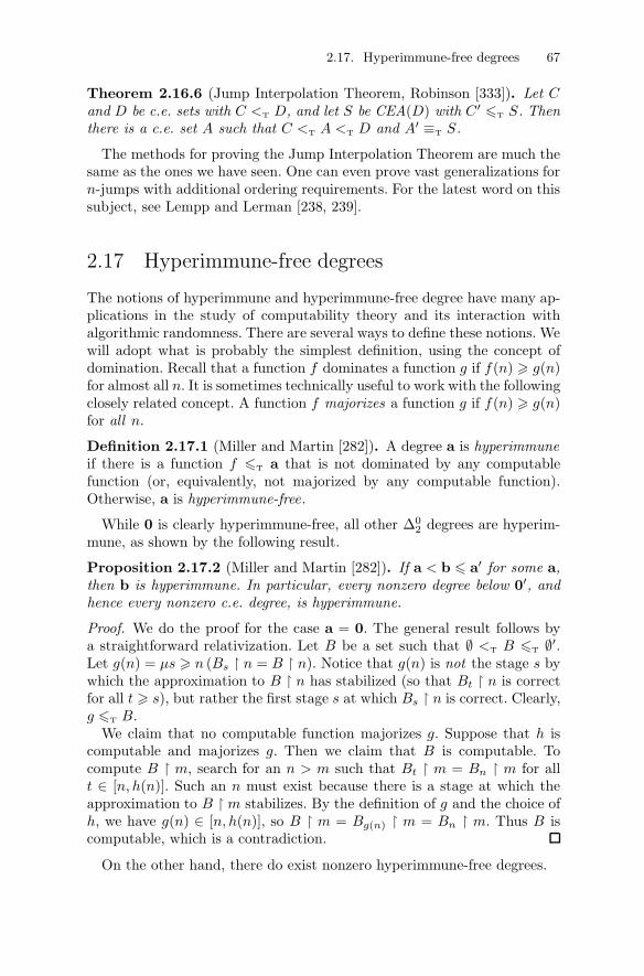
2.17. Hyperimmune-free degrees 67
Theorem 2.16.6 (Jump Interpolation Theorem, Robinson [333]). Let Cand D be c.e. sets with C <T D, and let S be CEA(D) with C′ �T S. Thenthere is a c.e. set A such that C <T A <T D and A′ ≡T S.
The methods for proving the Jump Interpolation Theorem are much thesame as the ones we have seen. One can even prove vast generalizations forn-jumps with additional ordering requirements. For the latest word on thissubject, see Lempp and Lerman [238, 239].
2.17 Hyperimmune-free degrees
The notions of hyperimmune and hyperimmune-free degree have many ap-plications in the study of computability theory and its interaction withalgorithmic randomness. There are several ways to define these notions. Wewill adopt what is probably the simplest definition, using the concept ofdomination. Recall that a function f dominates a function g if f(n) � g(n)for almost all n. It is sometimes technically useful to work with the followingclosely related concept. A function f majorizes a function g if f(n) � g(n)for all n.
Definition 2.17.1 (Miller and Martin [282]). A degree a is hyperimmuneif there is a function f �T a that is not dominated by any computablefunction (or, equivalently, not majorized by any computable function).Otherwise, a is hyperimmune-free.
While 0 is clearly hyperimmune-free, all other Δ02 degrees are hyperim-
mune, as shown by the following result.
Proposition 2.17.2 (Miller and Martin [282]). If a < b � a′ for some a,then b is hyperimmune. In particular, every nonzero degree below 0′, andhence every nonzero c.e. degree, is hyperimmune.
Proof. We do the proof for the case a = 0. The general result follows bya straightforward relativization. Let B be a set such that ∅ <T B �T ∅′.Let g(n) = μs � n (Bs � n = B � n). Notice that g(n) is not the stage s bywhich the approximation to B � n has stabilized (so that Bt � n is correctfor all t � s), but rather the first stage s at which Bs � n is correct. Clearly,g �T B.
We claim that no computable function majorizes g. Suppose that h iscomputable and majorizes g. Then we claim that B is computable. Tocompute B � m, search for an n > m such that Bt � m = Bn � m for allt ∈ [n, h(n)]. Such an n must exist because there is a stage at which theapproximation to B � m stabilizes. By the definition of g and the choice ofh, we have g(n) ∈ [n, h(n)], so B � m = Bg(n) � m = Bn � m. Thus B iscomputable, which is a contradiction.
On the other hand, there do exist nonzero hyperimmune-free degrees.
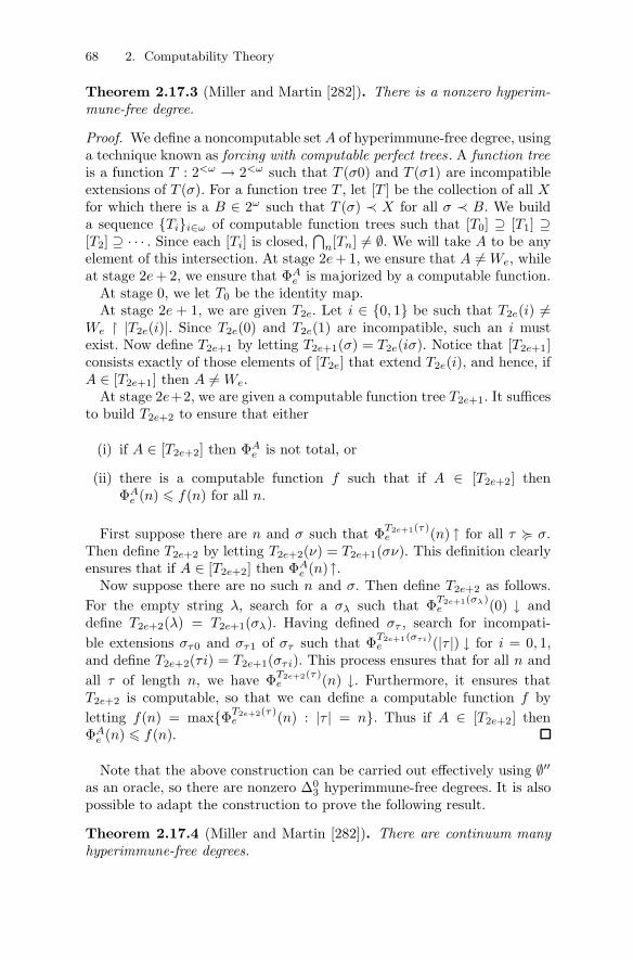
68 2. Computability Theory
Theorem 2.17.3 (Miller and Martin [282]). There is a nonzero hyperim-mune-free degree.
Proof. We define a noncomputable set A of hyperimmune-free degree, usinga technique known as forcing with computable perfect trees . A function treeis a function T : 2<ω → 2<ω such that T (σ0) and T (σ1) are incompatibleextensions of T (σ). For a function tree T , let [T ] be the collection of all Xfor which there is a B ∈ 2ω such that T (σ) ≺ X for all σ ≺ B. We builda sequence {Ti}i∈ω of computable function trees such that [T0] ⊇ [T1] ⊇[T2] ⊇ · · · . Since each [Ti] is closed,
⋂n[Tn] �= ∅. We will take A to be any
element of this intersection. At stage 2e+ 1, we ensure that A �= We, whileat stage 2e+ 2, we ensure that ΦAe is majorized by a computable function.
At stage 0, we let T0 be the identity map.At stage 2e + 1, we are given T2e. Let i ∈ {0, 1} be such that T2e(i) �=
We � |T2e(i)|. Since T2e(0) and T2e(1) are incompatible, such an i mustexist. Now define T2e+1 by letting T2e+1(σ) = T2e(iσ). Notice that [T2e+1]consists exactly of those elements of [T2e] that extend T2e(i), and hence, ifA ∈ [T2e+1] then A �= We.
At stage 2e+2, we are given a computable function tree T2e+1. It sufficesto build T2e+2 to ensure that either
(i) if A ∈ [T2e+2] then ΦAe is not total, or
(ii) there is a computable function f such that if A ∈ [T2e+2] thenΦAe (n) � f(n) for all n.
First suppose there are n and σ such that ΦT2e+1(τ)e (n) ↑ for all τ � σ.
Then define T2e+2 by letting T2e+2(ν) = T2e+1(σν). This definition clearlyensures that if A ∈ [T2e+2] then ΦAe (n)↑.
Now suppose there are no such n and σ. Then define T2e+2 as follows.For the empty string λ, search for a σλ such that ΦT2e+1(σλ)
e (0) ↓ anddefine T2e+2(λ) = T2e+1(σλ). Having defined στ , search for incompati-ble extensions στ0 and στ1 of στ such that ΦT2e+1(στi)
e (|τ |) ↓ for i = 0, 1,and define T2e+2(τi) = T2e+1(στi). This process ensures that for all n andall τ of length n, we have ΦT2e+2(τ)
e (n) ↓. Furthermore, it ensures thatT2e+2 is computable, so that we can define a computable function f byletting f(n) = max{ΦT2e+2(τ)
e (n) : |τ | = n}. Thus if A ∈ [T2e+2] thenΦAe (n) � f(n).
Note that the above construction can be carried out effectively using ∅′′as an oracle, so there are nonzero Δ0
3 hyperimmune-free degrees. It is alsopossible to adapt the construction to prove the following result.
Theorem 2.17.4 (Miller and Martin [282]). There are continuum manyhyperimmune-free degrees.

2.17. Hyperimmune-free degrees 69
On the other hand, we will see in Section 8.21.1 that the class of sets ofhyperimmune-free degree has measure 0.
The name “hyperimmune degree” comes from the notion of a hyperim-mune set, which we now define.9 A strong array is a computable collectionof pairwise disjoint finite sets {Fi}i∈N (which means not only that the Fiare uniformly computable, but also that the function i → maxFi is com-putable). An infinite set A is hyperimmune if for all strong arrays {Fi}i∈N,there is an i such that Fi ⊂ A. A c.e. set is hypersimple if its complementis hyperimmune.
Given the terminology, one would expect that a hyperimmune degree isone that contains a hyperimmune set. We will show that this is indeed thecase by first introducing another equivalent characterization of the hyper-immune degrees. The principal function of a set A = {a0 < a1 < · · · } isthe function pA defined by pA(n) = an.
Lemma 2.17.5 (Miller and Martin [282]). A degree a is hyperimmune iff acontains a set A such that pA is not majorized by any computable function.
Proof. Since pA �T A, the “if” direction is obvious. For the other direction,suppose that there is a function f �T a that is not majorized by anycomputable function. We may assume that f is increasing. Let B ∈ a andlet b0 < b1 < · · · be the elements of B. Let A = {f(bn) : n ∈ N}. Usingthe fact that f is increasing, it is easy to show that A ≡T B. Thus A ∈ a,and pA(n) � f(n) for all n, so pA is not majorized by any computablefunction.
Theorem 2.17.6 (Kuznecov [230], Medvedev [264], Uspensky [393]). Adegree is hyperimmune iff it contains a hyperimmune set.
Proof. Suppose that A is not hyperimmune. Then there is a strong array{Fi}i∈N such that A ∩ Fi �= ∅ for all i. Let f(n) = max
⋃i�n Fi. Then f is
computable, and pA(n) � f(n) for all n. So if no set in a is hyperimmune,then it follows from Lemma 2.17.5 that a is not hyperimmune.
Now suppose that a is not hyperimmune and let A ∈ a. By Lemma2.17.5, there is a computable function f such that pA(n) � f(n) for all n.Let F0 = [0, f(0)]. Given Fi, let ki = maxFi + 1 and let Fi+1 = [ki, f(ki)].Then pA(ki) ∈ A ∩ Fi for all i, so A is not hyperimmune.
The following is a useful characterization of the hyperimmune-freedegrees.
9Some authors have argued that the adoption of the term “hyperimmune-free degree”is a historical accident, and that a more descriptive one, based on domination properties,should be used. Nies, Barmpalias, and Soare, for example, have all used the term com-putably dominated. Earlier, authors such as Gasarch and Simpson used the term almostrecursive.

70 2. Computability Theory
Proposition 2.17.7 (Jockusch [187], Martin [unpublished]). The followingare equivalent for a set A.
(i) A has hyperimmune-free degree.
(ii) For all functions f , if f �T A then f �tt A.
(iii) For all sets B, if B �T A then B �tt A.
Proof. To show that (i) implies (ii), suppose that A has hyperimmune-freedegree and f = ΦAe , and let g(n) be the number of steps taken by thecomputation ΦAe (n). Then g �T A, so there is a computable function hthat majorizes g. Let Ψ be the functional defined as follows. On oracleX and input n, run the computation ΦXe (n) for h(n) many steps. If thiscomputation converges, then output its value, and otherwise output 0. ThenΨ is a truth table functional, and ΨA = ΦAe = f .
Clearly (ii) implies (iii). To show that (iii) implies (i), assume that Adoes not have hyperimmune-free degree and let g �T A be a function notdominated by any computable function. We build a set B �T A such thatB �tt A. Let σ0, σ1, . . . be an effective list of all truth tables. For eache and n, proceed as follows. If Φe(〈e, n〉)[g(n)] ↓ then let 〈e, n〉 ∈ B iffA � σΦe(〈e,n〉). Note that this definition ensures that Φe does not witness atruth table reduction from A to B. If Φe(〈e, n〉)[g(n)]↑ then let 〈e, n〉 ∈ B.Clearly B �T A. Assume for a contradiction that B �tt A. Then there is ane such that Φe witnesses this fact. This Φe is total, so there is a computablefunction h such that Φe(〈e, n〉)[h(n)]↓ for all n. Since h does not dominateg, there is an n such that Φe(〈e, n〉)[g(n)]↓. For this n, we have 〈e, n〉 ∈ Biff A � σΦe(〈e,n〉), contradicting the choice of e.
The above result cannot be extended to wtt-reducibility. Downey [99]constructed a noncomputable c.e. set A such that for all sets B, if B �T Athen B �wtt A. Since A is noncomputable and c.e., it has hyperimmunedegree.
2.18 Minimal degrees
The proof of Theorem 2.17.3 uses ideas that go back to a fundamentaltheorem of Spector [374].
Definition 2.18.1. A degree a > 0 is minimal if there is no degree b with0 < b < a.
Theorem 2.18.2 (Spector [374]). There is a minimal degree below 0′′.
Proof. As with Theorem 2.17.3, the proof uses forcing with computableperfect trees. As before, we build a sequence {Ti}i∈ω of computable functiontrees such that [T0] ⊇ [T1] ⊇ [T2] ⊇ · · · , and take our set A of minimaldegree to be any element of
⋂n[Tn].
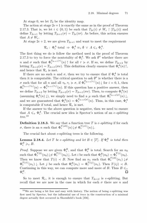
2.18. Minimal degrees 71
At stage 0, we let T0 be the identity map.The action at stage 2e+1 is exactly the same as in the proof of Theorem
2.17.3. That is, we let i ∈ {0, 1} be such that T2e(i) �= We � |T2e(i)| anddefine T2e+1 by letting T2e+1(σ) = T2e(iσ). As before, this action ensuresthat A �= We.
At stage 2e+ 2, we are given T2e+1 and want to meet the requirement
Re : ΦAe total ⇒ ΦAe ≡T ∅ ∨ A �T ΦAe .
The first thing we do is follow the method used in the proof of Theorem2.17.3 to try to force the nontotality of ΦAe . We ask ∅′′ whether there aren and σ such that ΦT2e+1(τ)
e (n) ↑ for all τ � σ. If so, we define T2e+2 byletting T2e+2(ν) = T2e+1(σν). This definition clearly ensures that ΦAe (n)↑,and hence that Re is met.
If there are no such n and σ, then we try to ensure that if ΦAe is totalthen it is computable. The critical question to ask ∅′′ is whether there is aσ such that for all n and all τ0, τ1 � σ, if ΦT2e+1(τi)
e (n)↓ for i = 0, 1, thenΦT2e+1(τ0)e (n) = ΦT2e+1(τ1)
e (n). If this question has a positive answer, thenwe define T2e+2 by letting T2e+2(ν) = T2e+1(σν). Then, to compute ΦAe (n)(assuming ΦAe (n) ↓), we simply need to find a μ such that ΦT2e+2(μ)
e (n) ↓,and we are guaranteed that ΦAe (n) = ΦT2e+2(μ)
e (n). Thus, in this case, ΦAeis computable if total, and hence Re is met.
If the answer to the above question is negative, then we need to ensurethat A �T ΦAe . The crucial new idea is Spector’s notion of an e-splittingtree.10
Definition 2.18.3. We say that a function tree T is e-splitting if for eachσ, there is an n such that ΦT (σ0)
e (n)↓�= ΦT (σ1)e (n)↓.
The crucial fact about e-splitting trees is the following.
Lemma 2.18.4. Let T be e-splitting and let B ∈ [T ]. If ΦBe is total thenΦBe �T B.
Proof. Suppose we are given ΦBe , and that ΦBe is total. Search for an n0
such that ΦT (0)e (n0)↓�= ΦT (1)
e (n0)↓. Let i be such that ΦBe (n0) = ΦT (i)e (n0).
Then we know that T (i) ≺ B. Now find an n1 such that ΦT (i0)e (n1) ↓�=
ΦT (i1)e (n1) ↓. Let j be such that ΦBe (n1) = ΦT (ij)
e (n1). Then T (ij) ≺ B.Continuing in this way, we can compute more and more of B. Thus B �T
ΦBe .
So to meet Re, it is enough to ensure that T2e+2 is e-splitting. Butrecall that we are now in the case in which for each σ there are n and
10We are being a bit free and easy with history. The notion of being e-splitting wasfirst used by Spector, but the influential use of trees in the construction of a minimaldegree actually first occurred in Shoenfield’s book [356].
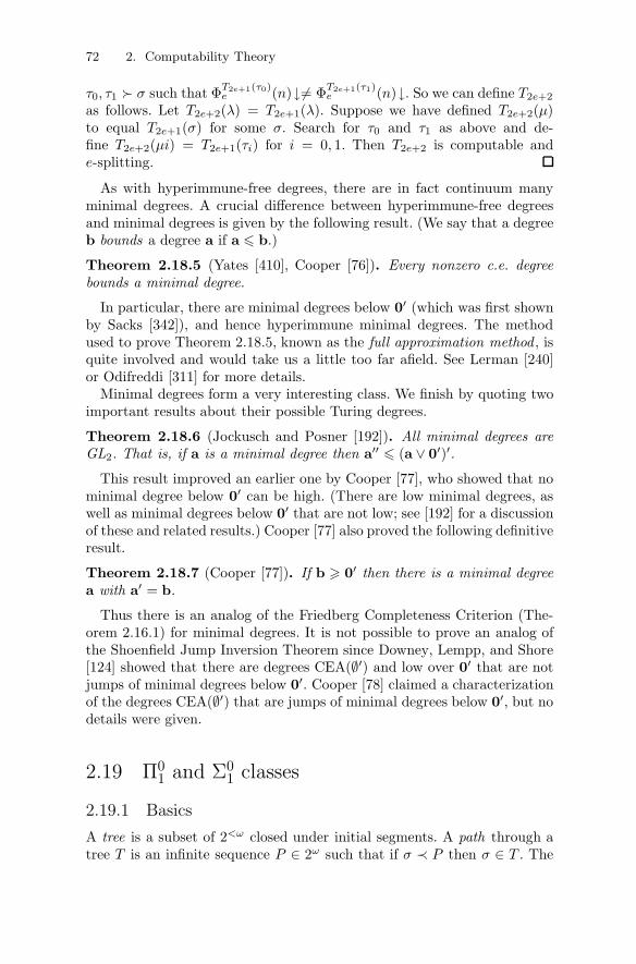
72 2. Computability Theory
τ0, τ1 � σ such that ΦT2e+1(τ0)e (n)↓�= ΦT2e+1(τ1)
e (n)↓. So we can define T2e+2
as follows. Let T2e+2(λ) = T2e+1(λ). Suppose we have defined T2e+2(μ)to equal T2e+1(σ) for some σ. Search for τ0 and τ1 as above and de-fine T2e+2(μi) = T2e+1(τi) for i = 0, 1. Then T2e+2 is computable ande-splitting.
As with hyperimmune-free degrees, there are in fact continuum manyminimal degrees. A crucial difference between hyperimmune-free degreesand minimal degrees is given by the following result. (We say that a degreeb bounds a degree a if a � b.)
Theorem 2.18.5 (Yates [410], Cooper [76]). Every nonzero c.e. degreebounds a minimal degree.
In particular, there are minimal degrees below 0′ (which was first shownby Sacks [342]), and hence hyperimmune minimal degrees. The methodused to prove Theorem 2.18.5, known as the full approximation method , isquite involved and would take us a little too far afield. See Lerman [240]or Odifreddi [311] for more details.
Minimal degrees form a very interesting class. We finish by quoting twoimportant results about their possible Turing degrees.
Theorem 2.18.6 (Jockusch and Posner [192]). All minimal degrees areGL2. That is, if a is a minimal degree then a′′ � (a ∨ 0′)′.
This result improved an earlier one by Cooper [77], who showed that nominimal degree below 0′ can be high. (There are low minimal degrees, aswell as minimal degrees below 0′ that are not low; see [192] for a discussionof these and related results.) Cooper [77] also proved the following definitiveresult.
Theorem 2.18.7 (Cooper [77]). If b � 0′ then there is a minimal degreea with a′ = b.
Thus there is an analog of the Friedberg Completeness Criterion (The-orem 2.16.1) for minimal degrees. It is not possible to prove an analog ofthe Shoenfield Jump Inversion Theorem since Downey, Lempp, and Shore[124] showed that there are degrees CEA(∅′) and low over 0′ that are notjumps of minimal degrees below 0′. Cooper [78] claimed a characterizationof the degrees CEA(∅′) that are jumps of minimal degrees below 0′, but nodetails were given.
2.19 Π01 and Σ0
1 classes
2.19.1 Basics
A tree is a subset of 2<ω closed under initial segments. A path through atree T is an infinite sequence P ∈ 2ω such that if σ ≺ P then σ ∈ T . The

2.19. Π01 and Σ0
1 classes 73
collection of paths through T is denoted by [T ]. A subset of 2ω is a Π01
class if it is equal to [T ] for some computable tree T .11
An equivalent formulation is that C is a Π01 class if there is a computable
relation R such that
C = {A ∈ 2ω : ∀nR(A � n)}.
It is not hard to show that this definition is equivalent to the one viacomputable trees.
There is a host of natural examples of important Π01 in several branches
of logic. For example, let A and B be disjoint c.e. sets. The collection ofseparating sets {X : X ⊇ A ∧ X ∩ B = ∅} is a Π0
1 class. An importantspecial case is an effectively inseparable pair, that is, a pair of disjoint c.e.sets A and B for which there is a computable function f such that for alldisjoint c.e. We ⊇ A and Wj ⊇ B, we have f(e, j) /∈ We ∪ Wj . This isthe two variable version of a creative set. One example of an effectivelyinseparable pair is the sets {e : Φe(e) ↓= 0} and {e : Φe(e) ↓= 1}. Thefunction f witnessing the effective inseparability of this pair is not hard tobuild: given e and j, using the recursion theorem we can find an i such thatΦi(i)↓= 1 if i ∈We and Φi(i)↓= 0 if i ∈Wj .12 We then let f(e, j) = i.
Another example of a Π01 class is the class of (codes of) extensions of a
complete consistent theory. By the proof of Godel’s Incompleteness Theo-rem (see e.g. [139]), for a theory such as Peano Arithmetic (PA), the setA of sentences provable from PA and the set B of sentences refutable fromPA form an effectively inseparable pair.
It is easy to check that the intersection of two Π01 classes is again a Π0
1
class, as is their union.The complement of a Π0
1 class is a Σ01 class . Thus C is a Σ0
1 class iff thereis a computable relation R such that
C = {A : ∃nR(A � n)}.
We can think of Σ01 classes as the analogs for infinite sequences of c.e. sets
of finite strings. Indeed, an important fact about Σ01 classes is that they
are exactly the subsets of 2ω generated by c.e. sets of finite strings, in thefollowing sense. (Here we use the notation of Section 1.2.)
11Sometimes a Π01 class is defined to be the set of paths through a computable subtree
T of ω<ω . Such a class is computably bounded if there is a computable function f suchthat for each σ ∈ T , if σn ∈ T then n � f(σ). The study of computably boundedΠ0
1 classes reduces to the study of the special case of Π01 subclasses of 2ω , since every
computably bounded Π01 class is computably equivalent to a Π0
1 subclass of 2ω . We willrestrict our attention to such classes, so for us a Π0
1 class will mean a Π01 subclass of 2ω .
12In greater detail: Let g be a computable function such that for each k, the machineΦg(k) ignores its input and waits until k enters either We or Wj , at which point themachine returns 0 if k ∈ We and 1 if k ∈ Wj (while if k /∈ We ∪Wj then the machinedoes not return). By the recursion theorem, there is an i such that Φi = Φg(i). For thisi, we have Φi(i)↓= 1 if i ∈ We and Φi(i)↓= 0 if i ∈ Wj .
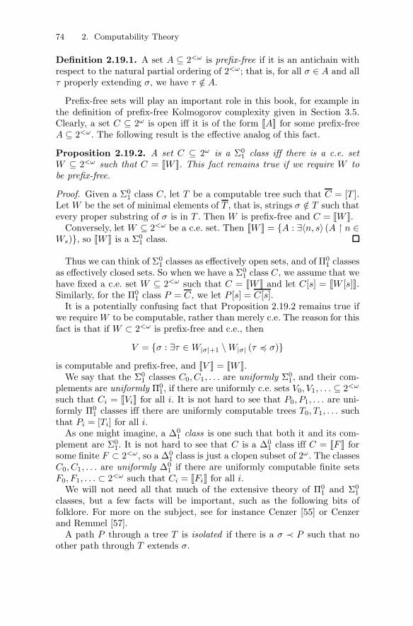
74 2. Computability Theory
Definition 2.19.1. A set A ⊆ 2<ω is prefix-free if it is an antichain withrespect to the natural partial ordering of 2<ω; that is, for all σ ∈ A and allτ properly extending σ, we have τ /∈ A.
Prefix-free sets will play an important role in this book, for example inthe definition of prefix-free Kolmogorov complexity given in Section 3.5.Clearly, a set C ⊆ 2ω is open iff it is of the form �A� for some prefix-freeA ⊆ 2<ω. The following result is the effective analog of this fact.
Proposition 2.19.2. A set C ⊆ 2ω is a Σ01 class iff there is a c.e. set
W ⊆ 2<ω such that C = �W �. This fact remains true if we require W tobe prefix-free.
Proof. Given a Σ01 class C, let T be a computable tree such that C = [T ].
Let W be the set of minimal elements of T , that is, strings σ /∈ T such thatevery proper substring of σ is in T . Then W is prefix-free and C = �W �.
Conversely, let W ⊆ 2<ω be a c.e. set. Then �W � = {A : ∃〈n, s〉 (A � n ∈Ws)}, so �W � is a Σ0
1 class.
Thus we can think of Σ01 classes as effectively open sets, and of Π0
1 classesas effectively closed sets. So when we have a Σ0
1 class C, we assume that wehave fixed a c.e. set W ⊆ 2<ω such that C = �W � and let C[s] = �W [s]�.Similarly, for the Π0
1 class P = C, we let P [s] = C[s].It is a potentially confusing fact that Proposition 2.19.2 remains true if
we require W to be computable, rather than merely c.e. The reason for thisfact is that if W ⊂ 2<ω is prefix-free and c.e., then
V = {σ : ∃τ ∈ W|σ|+1 \W|σ| (τ � σ)}
is computable and prefix-free, and �V � = �W �.We say that the Σ0
1 classes C0, C1, . . . are uniformly Σ01, and their com-
plements are uniformly Π01, if there are uniformly c.e. sets V0, V1, . . . ⊆ 2<ω
such that Ci = �Vi� for all i. It is not hard to see that P0, P1, . . . are uni-formly Π0
1 classes iff there are uniformly computable trees T0, T1, . . . suchthat Pi = [Ti] for all i.
As one might imagine, a Δ01 class is one such that both it and its com-
plement are Σ01. It is not hard to see that C is a Δ0
1 class iff C = �F � forsome finite F ⊂ 2<ω, so a Δ0
1 class is just a clopen subset of 2ω. The classesC0, C1, . . . are uniformly Δ0
1 if there are uniformly computable finite setsF0, F1, . . . ⊂ 2<ω such that Ci = �Fi� for all i.
We will not need all that much of the extensive theory of Π01 and Σ0
1
classes, but a few facts will be important, such as the following bits offolklore. For more on the subject, see for instance Cenzer [55] or Cenzerand Remmel [57].
A path P through a tree T is isolated if there is a σ ≺ P such that noother path through T extends σ.

2.19. Π01 and Σ0
1 classes 75
Proposition 2.19.3. Let T be a computable tree and let P be an isolatedpath through T . Then P is computable.
Proof. Let σ ≺ P be such that no path through T other than P extends σ.For any n > |σ|, there is exactly one τ � σ such that the portion of T aboveτ is infinite (by Konig’s Lemma, which says that if a finitely branching treeis infinite, then it has a path). So to compute P � n for n > |σ|, we lookfor an m � n such that exactly one τ � σ of length n has an extension oflength m in T . Then P � n = τ .
Corollary 2.19.4. Let C be a Π01 class with only finitely many members.
Then every member of C is computable.
Proof. Let T be a computable tree such that C = [T ]. Then T has onlyfinitely many paths, so every path through T is isolated.
Proposition 2.19.5. Let C be a nonempty Π01 class with no computable
members. Then |C| = 2ℵ0 .
Proof. Let T be a computable tree such that C = [T ]. Let S be the set ofextendible elements of T , that is, those σ such that there is an extensionof σ in [T ]. If every σ ∈ S has two incompatible extensions in S, then it iseasy to show that there are continuum many paths through T . Otherwise,there is a σ ∈ S with a unique extension P ∈ [T ]. As in the previous proof,P is computable.
Note also that the question of whether a given computable tree T is finiteis an existential one, since it amounts to asking whether there is an n suchthat no string of length n is in T , and hence it can be decided by ∅′.
The Cantor-Bendixson derivative of a Π01 class C is the class C′ obtained
from C by removing the isolated points of C (i.e., those elements X ∈ Csuch that for some n, we have �X � n� ∩ C = {X}). Let C(0) = C. For anordinal δ, let C(δ+1) = (Cδ)′, and for a limit ordinal δ, let C(δ) =
⋂γ<δ C
(γ).The rank of X ∈ C is the least δ such that X ∈ C(δ) \ C(δ+1), if sucha δ exists. Note that, by Proposition 2.19.3, if X has rank 0, then it iscomputable. If all the elements of C have ranks, then the rank of C is thesupremum of the ranks of its elements (or, equivalently, the least δ suchthat C(δ+1) = ∅).
2.19.2 Π0n and Σ0
n classes
There is a hierarchy of classes, akin to the arithmetic hierarchy of sets.
Definition 2.19.6. A set C ⊆ 2ω is a Π0n class if there is a computable
relation R such that
C = {A : ∀k1 ∃k2 · · ·QknR(A � k1, A � k2, . . . , A � kn)},

76 2. Computability Theory
where the quantifiers alternate and hence Q = ∀ if n is odd and Q = ∃ ifn is even.
The complement of a Π0n class is a Σ0
n class .
These definitions can be relativized to a given set X (by letting Rbe X-computable) to obtain the notions of Π0,X
n class and Σ0,Xn class.
A Π0n+1 class is also a Π0,∅(n)
1 class, since every predicate of the form∃k2 · · ·QknR(A � k1, A � k2, . . . , A � kn) with R computable is computablein ∅(n). Similarly, every Σ0
n+1 class is also a Σ0,∅(n)
1 class. The converse,however, is not always true, because every Π0,∅′
1 class is closed (indeed,every Π0,X
1 class is closed for any X), but there are Π02 classes that are not
closed, such as the class C of all A with A(m) = 1 for infinitely many m,which can be written as {A : ∀k ∃m (m > k ∧ A(m) = 1)}.
Indeed, even a closed Π02 class can fail to be a Π0,∅′
1 class. Doug Cenzer[personal communication] provided us the following example. It is not hardto build a computable subtree T of N<ω with a single infinite path f �T ∅′.Let T = {1n0+101n1+10 . . . 1nk+10m : (n0, . . . , nk) ∈ T, m ∈ N}. It is easyto check that T is a computable subtree of 2<ω. Let P = [T ] ∩ C, whereC is as in the previous paragraph. Then P is a Π0
2 class (because, as withΠ0
1 classes, the intersection of two Π0n classes is again a Π0
n class, as is theirunion). Furthermore, P has a single member A = 1f(0)+101f(1)+10 . . . . ButA ≡T f , so A �T ∅′. Thus P cannot be a Π0,∅′
1 class by the relativized formof Corollary 2.19.4.
Since Σ0,∅(n)
1 sets are the same as Σ0n sets, the relativized form of Propo-
sition 2.19.2 says that a class is Σ0,∅(n)
1 iff it is of the form �W � for someΣ0n set W ⊆ 2<ω.We fix effective listings Sn0 , Sn1 , . . . of the Σ0
n classes by letting Sne = {A :∃k1 ∀k2 · · ·QknR(A � k1, A � k2, . . . , A � kn)} where e is a code for then-ary computable relation R. By an index for a Σ0
n class S we mean an isuch that S = Sni . Similarly, by an index for a Π0
n class P we mean an isuch that P = Sni . We do the same for relativized classes in the naturalway. We then say that the classes C0, C1, . . . are uniformly Σ0
n if thereis a computable function f such that Ci = Snf(i) for all i, and uniformlyΠ0n if their complements are uniformly Σ0
n. This definition agrees with thedefinition of uniformly Σ0
1 classes given in the previous section because theproof of Proposition 2.19.2 is effective, as we now note.
Proposition 2.19.7. From an index for a Σ01 class C, we can computably
find an index for a (prefix-free) c.e. set W ⊆ 2<ω such that C = �W �, andvice versa.
Another way to look at this hierarchy of classes is in terms of effectiveunions and intersections. For example, in the same way that Π0
1 and Σ01
classes are the effective analogs of closed and open sets, respectively, Π02
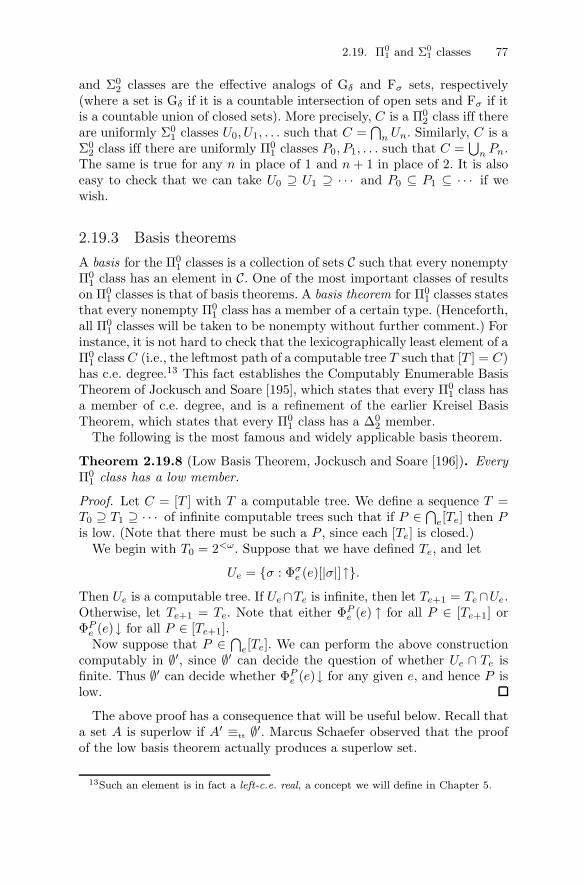
2.19. Π01 and Σ0
1 classes 77
and Σ02 classes are the effective analogs of Gδ and Fσ sets, respectively
(where a set is Gδ if it is a countable intersection of open sets and Fσ if itis a countable union of closed sets). More precisely, C is a Π0
2 class iff thereare uniformly Σ0
1 classes U0, U1, . . . such that C =⋂n Un. Similarly, C is a
Σ02 class iff there are uniformly Π0
1 classes P0, P1, . . . such that C =⋃n Pn.
The same is true for any n in place of 1 and n+ 1 in place of 2. It is alsoeasy to check that we can take U0 ⊇ U1 ⊇ · · · and P0 ⊆ P1 ⊆ · · · if wewish.
2.19.3 Basis theorems
A basis for the Π01 classes is a collection of sets C such that every nonempty
Π01 class has an element in C. One of the most important classes of results
on Π01 classes is that of basis theorems. A basis theorem for Π0
1 classes statesthat every nonempty Π0
1 class has a member of a certain type. (Henceforth,all Π0
1 classes will be taken to be nonempty without further comment.) Forinstance, it is not hard to check that the lexicographically least element of aΠ0
1 class C (i.e., the leftmost path of a computable tree T such that [T ] = C)has c.e. degree.13 This fact establishes the Computably Enumerable BasisTheorem of Jockusch and Soare [195], which states that every Π0
1 class hasa member of c.e. degree, and is a refinement of the earlier Kreisel BasisTheorem, which states that every Π0
1 class has a Δ02 member.
The following is the most famous and widely applicable basis theorem.
Theorem 2.19.8 (Low Basis Theorem, Jockusch and Soare [196]). EveryΠ0
1 class has a low member.
Proof. Let C = [T ] with T a computable tree. We define a sequence T =T0 ⊇ T1 ⊇ · · · of infinite computable trees such that if P ∈
⋂e[Te] then P
is low. (Note that there must be such a P , since each [Te] is closed.)We begin with T0 = 2<ω. Suppose that we have defined Te, and let
Ue = {σ : Φσe (e)[|σ|]↑}.
Then Ue is a computable tree. If Ue∩Te is infinite, then let Te+1 = Te∩Ue.Otherwise, let Te+1 = Te. Note that either ΦPe (e) ↑ for all P ∈ [Te+1] orΦPe (e)↓ for all P ∈ [Te+1].
Now suppose that P ∈⋂e[Te]. We can perform the above construction
computably in ∅′, since ∅′ can decide the question of whether Ue ∩ Te isfinite. Thus ∅′ can decide whether ΦPe (e)↓ for any given e, and hence P islow.
The above proof has a consequence that will be useful below. Recall thata set A is superlow if A′ ≡tt ∅′. Marcus Schaefer observed that the proofof the low basis theorem actually produces a superlow set.
13Such an element is in fact a left-c.e. real, a concept we will define in Chapter 5.

78 2. Computability Theory
Corollary 2.19.9 (Jockusch and Soare [196], Schaefer). Every Π01 class
has a superlow member.
The following variation on the low basis theorem will be useful below.
Theorem 2.19.10 (Jockusch and Soare [196]). Let C be a Π01 class and
let X be a noncomputable set. Then there is an A ∈ C such that X �T Aand A′ �T X ⊕ ∅′.
Proof. Let C = [T ] with T a computable tree. As in the proof of thelow basis theorem, we define a sequence T = T0 ⊇ T1 ⊇ · · · of infinitecomputable trees.
We begin with T0 = 2<ω. Suppose that we have defined T2e to be acomputable tree. We first proceed as in the proof of the low basis theorem.Let Ue = {σ : Φσe (e)[|σ|]↑}. If Ue∩T2e is infinite, then let T2e+1 = T2e∩Ue.Otherwise, let T2e+1 = T2e. As before, T2e+1 is a computable tree.
We now handle cone-avoidance as follows. We X⊕∅′-computably searchuntil we find that one of the following holds.
1. There are an n and an extendible σ ∈ T2e+1 such that Φσe (n)↓�= X(n).
2. There is an n such that T2e+1 ∩ {σ : Φσe (n)↑} is infinite.
We claim one of the above must hold. Suppose not, and fix n. The factthat 2 does not hold means that we can find a k such that Φσe (n)↓ for allσ ∈ T2e+1 ∩ 2k. The fact that 1 does not hold means that, for each such σ,if Φσe (n) �= X(n), then T2e+1 is finite above σ. Thus we can compute X(n)by searching for a j such that for all σ, τ ∈ T2e+1 ∩ 2j , we have Φσe (n) ↓=Φτe(n)↓, which by the above must exist. Since X is noncomputable, either 1or 2 must hold. If we find that 1 holds, then let T2e+2 = T2e+1∩{τ : σ � τ}.Otherwise, let T2e+2 = T2e+1 ∩ {σ : Φσe (n)↑}.
Now let A ∈⋂e[Te]. It is easy to check that we can perform the above
construction computably in X ⊕ ∅′, so as in the proof of the low basistheorem, we have A′ �T X ⊕ ∅′. Furthermore, the definition of the treesT2e+2 ensures that X �T A.
Corollary 2.19.9 and Theorem 2.19.10 cannot be combined. That is, thereare a Π0
1 class C and a noncomputable set X such that X is computablefrom every superlow member of C. We will see examples in Section 14.4.
Another important basis theorem is provided by the hyperimmune-freedegrees.
Theorem 2.19.11 (Hyperimmune-Free Basis Theorem, Jockusch andSoare [196]). Every Π0
1 class has a member of hyperimmune-free degree.
Proof. Let C be a Π01 class, and let T be a computable tree such that
C = [T ]. We can carry out a construction like that in the proof of Millerand Martin’s Theorem 2.17.3 within T . We begin with T0 = T . We donot need the odd stages of that construction since we do not need to force

2.19. Π01 and Σ0
1 classes 79
noncomputability (as 0 is hyperimmune-free). Thus we deal with Φe atstage e+ 1.
We are given Te and we want to build Te+1 to ensure that either
(i) if A ∈ [Te+1] then ΦAe is not total, or
(ii) there is a computable function f such that if A ∈ [Te+1] then ΦAe (n) �f(n) for all n.
Let
Une = {σ : Φσe (n)↑}.
There are two cases.If there is an n such that Une ∩ Te is infinite, then let Te+1 = Une ∩ Te. In
this case, if A ∈ [Te+1] then ΦAe (n)↑.Otherwise, let Te+1 = Te. In this case, for each n we can compute a
number l(n) such that no string σ ∈ Te of length l(n) is in Une . For anysuch σ, we have Φσe (n)↓. Define the computable function f by
f(n) = max{Φσe (n) : σ ∈ Te ∧ |σ| = l(n)}.
Then A ∈ [Te+1] implies that ΦAe (n) � f(n) for all n.So if we let A ∈
⋂e[Te], then A is a member of C and has hyperimmune-
free degree.
In the above construction, if [T ] has no computable members, thenProposition 2.19.5 implies that each Te must have size 2ℵ0 . It is not hardto adjust the construction in this case to obtain continuum many membersof C of hyperimmune-free degree. Thus, a Π0
1 class with no computablemembers has continuum many members of hyperimmune-free degree.
The following result is an immediate consequence of the hyperimmune-free basis theorem and Theorem 2.17.2, but it was first explicitly articulatedby Kautz [200], who gave an interesting direct proof. Recall that a set A iscomputably enumerable in and above a set X (CEA(X)) if A is c.e. in Xand X �T A. A set A is CEA if it is CEA(X) for some X <T A.
Corollary 2.19.12 (Jockusch and Soare [196], Kautz [200]). Every Π01
class has a member that is not CEA.
Although the existence of minimal degrees (Theorem 2.18.2) was provedby techniques similar to those used to prove the hyperimmune-free basistheorem, there is no “minimal basis theorem”, since there are Π0
1 classeswith no members of minimal degree. An example is the Π0
1 class of all com-plete extensions of Peano Arithmetic, by Theorem 2.21.9 below. However,using techniques beyond the scope of this book, Groszek and Slaman [173]proved the following elegant result.
Theorem 2.19.13 (Groszek and Slaman [173]). There is a Π01 class such
that every member either is c.e. and noncomputable, or has minimal degree.

80 2. Computability Theory
We end this section by looking at examples of nonbasis theorems.
Proposition 2.19.14. The intersection of all bases for the Π01 classes is
the collection of computable sets, and hence there is no minimal basis.
Proof. If A is a computable set then {A} is a Π01 class, so every basis for
the Π01 classes must include A. On the other hand, if B is noncomputable
then, by Corollary 2.19.4, {B} is not a Π01 class, so every Π0
1 class mustcontain a member other than B, and hence the collection of all sets otherthan B is a basis for the Π0
1 classes.14
For our next result, we will need the following definition and lemma.
Definition 2.19.15. An infinite set A is effectively immune if there is acomputable function f such that for all e, if We ⊆ A then |We| � f(e).
Post gave the following construction of an effectively immune co-c.e. setA. At stage s, for each e < s, if We[s] ⊆ As and there is an x ∈ We[s] suchthat x > 2e, then put the least such x into A. Then A is infinite, and iseffectively immune via the function e → 2e.
Lemma 2.19.16 (Martin [258]). If a c.e. set B computes an effectivelyimmune set, then B is Turing complete.
Proof. Let B be c.e., and let A �T B be effectively immune, as witnessedby the computable function f . Let Γ be a reduction such that ΓB = A.
For each k we build a c.e. set Wh(k), where the computable function h isgiven by the recursion theorem with parameters. Initially, Wh(k) is empty.If k enters ∅′ at stage t then we wait until a stage s � t at which there is aq such that ΓB(n)[s]↓ for all n < q and there are more than f(h(k)) manynumbers in ΓB[s] � q. We then let Wh(k) = ΓB[s] � q.15 This action ensuresthat |Wh(k)| > f(h(k)), so we must have Wh(k) � A. Thus,
ΓB[s] � q = Wh(k) �= A � q = ΓB � q.
So to compute ∅′(k) from B, we simply look for a stage s at which thereis a q such that Bs � γB(n)[s] = B � γB(n)[s] for all n < q and there aremore than f(h(k)) many numbers in ΓB [s] � q. If k is not in ∅′ by stage s,it cannot later enter ∅′.
14Another way to prove this fact is to note that, by Theorem 2.17.2, the only sets thatare both low and hyperimmune-free are the computable ones.
15In greater detail: For each i and k, we define a c.e. set Ci,k as follows. Initially, Ci,k
is empty. If k enters ∅′ at stage t then we wait until a stage s � t at which there isa q such that ΓB(n)[s] ↓ for all n < q and there are more than f(i) many numbers inΓB [s] � q. We then let Ci,k = ΓB [s] � q. It is easy to see that there is a computablefunction g such that g(i, k) is an index for Ci,k for all i and k. By the recursion theoremwith parameters, there is a computable function h such that Wh(k) = Wg(h(k),k) for allk. This h has the required properties.
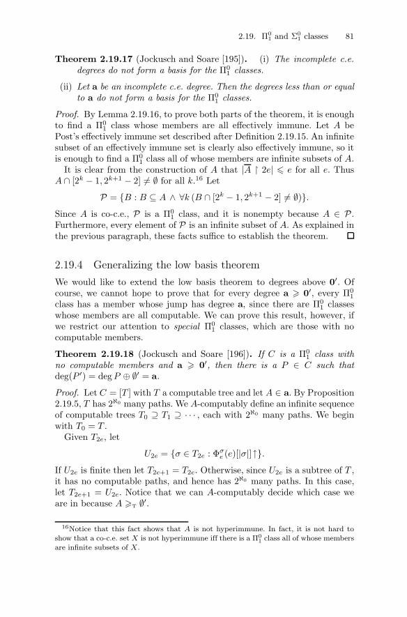
2.19. Π01 and Σ0
1 classes 81
Theorem 2.19.17 (Jockusch and Soare [195]). (i) The incomplete c.e.degrees do not form a basis for the Π0
1 classes.
(ii) Let a be an incomplete c.e. degree. Then the degrees less than or equalto a do not form a basis for the Π0
1 classes.
Proof. By Lemma 2.19.16, to prove both parts of the theorem, it is enoughto find a Π0
1 class whose members are all effectively immune. Let A bePost’s effectively immune set described after Definition 2.19.15. An infinitesubset of an effectively immune set is clearly also effectively immune, so itis enough to find a Π0
1 class all of whose members are infinite subsets of A.It is clear from the construction of A that |A � 2e| � e for all e. Thus
A ∩ [2k − 1, 2k+1 − 2] �= ∅ for all k.16 Let
P = {B : B ⊆ A ∧ ∀k (B ∩ [2k − 1, 2k+1 − 2] �= ∅)}.Since A is co-c.e., P is a Π0
1 class, and it is nonempty because A ∈ P .Furthermore, every element of P is an infinite subset of A. As explained inthe previous paragraph, these facts suffice to establish the theorem.
2.19.4 Generalizing the low basis theorem
We would like to extend the low basis theorem to degrees above 0′. Ofcourse, we cannot hope to prove that for every degree a � 0′, every Π0
1
class has a member whose jump has degree a, since there are Π01 classes
whose members are all computable. We can prove this result, however, ifwe restrict our attention to special Π0
1 classes, which are those with nocomputable members.
Theorem 2.19.18 (Jockusch and Soare [196]). If C is a Π01 class with
no computable members and a � 0′, then there is a P ∈ C such thatdeg(P ′) = degP ⊕ ∅′ = a.
Proof. Let C = [T ] with T a computable tree and let A ∈ a. By Proposition2.19.5, T has 2ℵ0 many paths. We A-computably define an infinite sequenceof computable trees T0 ⊇ T1 ⊇ · · · , each with 2ℵ0 many paths. We beginwith T0 = T .
Given T2e, let
U2e = {σ ∈ T2e : Φσe (e)[|σ|]↑}.If U2e is finite then let T2e+1 = T2e. Otherwise, since U2e is a subtree of T ,it has no computable paths, and hence has 2ℵ0 many paths. In this case,let T2e+1 = U2e. Notice that we can A-computably decide which case weare in because A �T ∅′.
16Notice that this fact shows that A is not hyperimmune. In fact, it is not hard toshow that a co-c.e. set X is not hyperimmune iff there is a Π0
1 class all of whose membersare infinite subsets of X.

82 2. Computability Theory
Now let σ0 <L σ1 be the length-lexicographically least pair of incompara-ble strings in T2e+1 such that for each i < 2, the subtree of T2e+1 above σiis infinite (and hence has 2ℵ0 many paths). Notice that we can find σ0, σ1
using A, again because A �T ∅′. Let T2e+2 be the subtree of T2e+1 aboveσA(e).
Having defined the Te, let P ∈⋂e[Te]. The choice of T2e+1 determines
whether ΦPe (e)↓, so, since the entire construction is A-computable, P ′ �T
A. On the other hand, we can also perform the construction (P ⊕ ∅′)-computably, since all the steps can be done ∅′-computably, except the choiceof which σi to extend in defining T2e+2, which can be done P -computably,since the σi we choose at that stage is the one extended by P . Furthermore,that choice determines the eth bit of A. Thus A �T P⊕∅′ �T P
′, and henceP ′ ≡T P ⊕ ∅′ ≡T A.
Corollary 2.19.19 (Jockusch and Soare [196]). For each a � 0′, the setswith degrees in {b : b′ = a} ∪ {0} form a basis for the Π0
1 classes.
2.20 Strong reducibilities and Post’s Program
The concept of hypersimplicity, which we defined in Section 2.17, was in-troduced by Post [316] as part of an attempt to solve Post’s Problem.Although hypersimple sets can be Turing complete, Post [316] showed thatno hypersimple set can be tt-complete. Later, Friedberg and Rogers [162]proved that no hypersimple set can be wtt-complete. This result has beenextended as follows. A set A is wtt-cuppable if there is a c.e. set W <wtt ∅′such that A⊕W �wtt ∅′.
Theorem 2.20.1 (Downey and Jockusch [119]). No hypersimple set iswtt-cuppable.
Proof. Suppose that A is hypersimple,W is c.e.,W �wtt ∅′, and A⊕W �wtt
∅′. We show that W �wtt ∅′. We will build a c.e. set B. By the recursiontheorem, we may assume that we have a wtt-reduction ΓA⊕W = B withcomputable use g.17 Without loss of generality, we may assume that g(n)is increasing and even for all n and write h(n) for g(n)
2 .We define a strong array {Fi}i∈N as follows, writing m(i) for maxFi.
Let F0 = [0, h(0)]. Given Fi, pick m(i) + 1 many fresh large numbersbi+10 < · · · < bi+1
m(i) and let Fi+1 = (maxFi, h(bi+1m(i))]. Since the Fi form a
strong array, there are infinitely many i with Fi ⊆ A. We can therefore
17In greater detail: We can think of the ensuing construction as building a c.e. setWf(e) given a parameter e, taking as Γ a wtt-functional such that ΓA⊕W = We. (It isnot hard to see that indices for Γ and for a computable function bounding its use can befound effectively from e.) By the recursion theorem, there is an e such that We = Wf(e),and we let B = We.
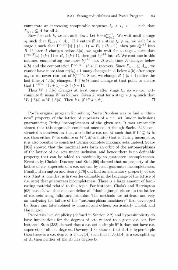
2.20. Strong reducibilities and Post’s Program 83
enumerate an increasing computable sequence i0 < i1 < · · · such thatFik+1 ⊆ A for all k.
Now for each k, we act as follows. Let b = bik+1m(ik). We wait until a stage
sk such that Fik+1 ⊆ Ask. If k enters ∅′ at a stage tk � sk, we wait for a
stage s such that ΓA⊕W [s] � (b + 1) = Bs � (b + 1), then put bik+10 into
B. If later A changes below h(b), we again wait for a stage s such thatΓA⊕W [s] � (b+1) = Bs � (b+1), then put bik+1
1 into B. We continue in thismanner, enumerating one more bik+1
j into B each time A changes belowh(b) and the computation ΓA⊕W � (b+ 1) recovers. Since Fik+1 ⊆ Ask
, wecannot have more than m(ik)+1 many changes in A below h(b) after stagesk, so we never run out of bik+1
j ’s. Since we change B � (b + 1) after thelast time A � h(b) changes, W � h(b) must change at that point to ensurethat ΓA⊕W � (b+ 1) = B � (b+ 1).
Thus W � h(b) changes at least once after stage tk, so we can wtt-compute ∅′ using W as follows. Given k, wait for a stage s � sk such thatWs � h(b) = W � h(b). Then k ∈ ∅′ iff k ∈ ∅′s.
Post’s original program for solving Post’s Problem was to find a “thin-ness” property of the lattice of supersets of a c.e. set (under inclusion)guaranteeing Turing incompleteness of the given set. It was eventuallyshown that this approach could not succeed. Although Sacks [343] con-structed a maximal set (i.e., a coinfinite c.e. set M such that if W ⊇ M isc.e. then either W is cofinite or W \M is finite) that is Turing incomplete,it is also possible to construct Turing complete maximal sets. Indeed, Soare[365] showed that the maximal sets form an orbit of the automorphismsof the lattice of c.e. sets under inclusion, and hence there is no definableproperty that can be added to maximality to guarantee incompleteness.Eventually, Cholak, Downey, and Stob [66] showed that no property of thelattice of c.e. supersets of a c.e. set can by itself guarantee incompleteness.Finally, Harrington and Soare [176] did find an elementary property of c.e.sets (that is, one that is first-order definable in the language of the lattice ofc.e. sets) that guarantees incompleteness. There is a large amount of fasci-nating material related to this topic. For instance, Cholak and Harrington[68] have shown that one can define all “double jump” classes in the latticeof c.e. sets using infinitary formulas. The methods are intricate and relyon analyzing the failure of the “automorphism machinery” first developedby Soare and later refined by himself and others, particularly Cholak andHarrington.
Properties like simplicity (defined in Section 2.2) and hypersimplicity dohave implications for the degrees of sets related to a given c.e. set. Forinstance, Stob [383] showed that a c.e. set is simple iff it does not have c.e.supersets of all c.e. degrees. Downey [100] showed that if A is hypersimplethen there is a c.e. degree b � deg(A) such that if A0 �A1 is a c.e. splittingof A, then neither of the Ai has degree b.
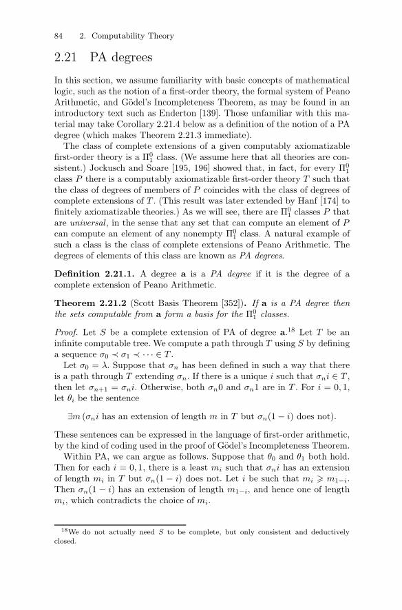
84 2. Computability Theory
2.21 PA degrees
In this section, we assume familiarity with basic concepts of mathematicallogic, such as the notion of a first-order theory, the formal system of PeanoArithmetic, and Godel’s Incompleteness Theorem, as may be found in anintroductory text such as Enderton [139]. Those unfamiliar with this ma-terial may take Corollary 2.21.4 below as a definition of the notion of a PAdegree (which makes Theorem 2.21.3 immediate).
The class of complete extensions of a given computably axiomatizablefirst-order theory is a Π0
1 class. (We assume here that all theories are con-sistent.) Jockusch and Soare [195, 196] showed that, in fact, for every Π0
1
class P there is a computably axiomatizable first-order theory T such thatthe class of degrees of members of P coincides with the class of degrees ofcomplete extensions of T . (This result was later extended by Hanf [174] tofinitely axiomatizable theories.) As we will see, there are Π0
1 classes P thatare universal , in the sense that any set that can compute an element of Pcan compute an element of any nonempty Π0
1 class. A natural example ofsuch a class is the class of complete extensions of Peano Arithmetic. Thedegrees of elements of this class are known as PA degrees.
Definition 2.21.1. A degree a is a PA degree if it is the degree of acomplete extension of Peano Arithmetic.
Theorem 2.21.2 (Scott Basis Theorem [352]). If a is a PA degree thenthe sets computable from a form a basis for the Π0
1 classes.
Proof. Let S be a complete extension of PA of degree a.18 Let T be aninfinite computable tree. We compute a path through T using S by defininga sequence σ0 ≺ σ1 ≺ · · · ∈ T .
Let σ0 = λ. Suppose that σn has been defined in such a way that thereis a path through T extending σn. If there is a unique i such that σni ∈ T ,then let σn+1 = σni. Otherwise, both σn0 and σn1 are in T . For i = 0, 1,let θi be the sentence
∃m (σni has an extension of length m in T but σn(1 − i) does not).
These sentences can be expressed in the language of first-order arithmetic,by the kind of coding used in the proof of Godel’s Incompleteness Theorem.
Within PA, we can argue as follows. Suppose that θ0 and θ1 both hold.Then for each i = 0, 1, there is a least mi such that σni has an extensionof length mi in T but σn(1 − i) does not. Let i be such that mi � m1−i.Then σn(1 − i) has an extension of length m1−i, and hence one of lengthmi, which contradicts the choice of mi.
18We do not actually need S to be complete, but only consistent and deductivelyclosed.

2.21. PA degrees 85
Thus PA � ¬(θ0 ∧ θ1), so there is a least i such that θ1−i /∈ S. Let σn+1 =σni. There must be a path through T extending σn+1, since otherwise wewould have PA � θ1−i, and hence θ1−i ∈ S.
In unpublished work, Solovay showed that, in fact, the property in The-orem 2.21.2 exactly characterizes the PA degrees. This fact, which we willstate as Corollary 2.21.4 below, follows immediately from the followingresult, which is important in its own right.
Theorem 2.21.3 (Solovay [unpublished]). The class of PA degrees isclosed upwards.
Proof. Let A be the set of (Godel numbers of) sentences provable in PA andB the set of (Godel numbers of) sentences refutable from PA. We followthe proof in Odifreddi [310], which uses the fact that A and B form aneffectively inseparable pair of c.e. sets (which recall means that there is acomputable function f such that for all disjoint c.e. We ⊇ A and Wi ⊇ B,we have f(e, i) /∈We ∪Wi).
Let T be a complete extension of PA computable in a set X . Using T ,we will build finite extensions Fσ of PA for σ ∈ 2<ω so that
⋃σ≺X Fσ is a
complete extension of PA with the same degree as X .Let ϕ0, ϕ1, . . . be an effective listing of the sentences of arithmetic. Let
Fλ = PA. Suppose that we have defined Fσ to be a finite consistent exten-sion of PA. Let ψ0 be an existential sentence of arithmetic expressing thestatement that
∃m (m codes a proof of ϕn in Fσand no k < m codes a proof of ¬ϕn in Fσ).
Let ψ1 be the same with the roles of ϕn and ¬ϕn interchanged.We have ψi ∈ T iff ψi is true, and at most one ψi is true. If ψ0 ∈ T then
let F ′σ = Fσ ∪ {ϕn} and otherwise let F ′
σ = Fσ ∪ {¬ϕn}.Let C be the sentences provable in F ′
σ and D the sentences refutablefrom F ′
σ. Then C and D are c.e. sets containing A and B, respectively,and we can effectively find indices for C and D. Since A and B form aneffectively inseparable pair, we can compute a sentence ν /∈ C ∪ D. LetFσ0 = F ′
σ ∪ {ν} and Fσ1 = F ′σ ∪ {¬ν}.
Let S =⋃σ≺X Fσ. Then S is a complete extension of PA, and is X-
computable, since T is X-computable. Given S, we can compute X asfollows. Assume by induction that we have computed X � n and FX�n. Weknow which of ϕn and ¬ϕn is in S, so we know F ′
X�n. Thus we can computeν. We know which of ν and ¬ν is in S, so we know X � n+ 1 and FX�n+1.Thus S ≡T X .
Since the complete extensions of PA form a Π01 class, if the sets com-
putable from a degree a form a basis for the Π01 classes, then in particular

86 2. Computability Theory
a computes a complete extension of PA, and hence, by the above theorem,is itself a PA degree. Thus we have the following result.
Corollary 2.21.4 (Solovay). A degree is PA iff the sets computable fromit form a basis for the Π0
1 classes.
A useful way to restate this corollary is that a degree a is PA iff everycomputable infinite subtree of 2<ω has an a-computable path.
Another way to characterize PA degrees is via effectively inseparablepairs of c.e. sets. Let A and B form such a pair. As previously mentioned,the class of all sets that separate A and B is a Π0
1 class, so every PA degreecomputes such a set. Conversely, given a set C separating A and B, wecan use the following useful lemma to obtain a C-computable completeextension of PA.
Lemma 2.21.5 (Muchnik [285], Smullyan [362]). Let C be a separatingset for an effectively inseparable pair of c.e. sets A and B, and let X andY be disjoint c.e. sets. Then there is a C-computable set separating X andY .
Proof. Let f be a total function witnessing the effective inseparability ofA and B. It is not hard to see that we may assume that f is 1-1. Using therecursion theorem with parameters, we can define computable 1-1 functionsg and h such that for all n we have
Wg(n) =
{A ∪ {f(g(n), h(n))} if n ∈ Y
A otherwise
and
Wh(n) =
{B ∪ {f(g(n), h(n))} if n ∈ X
B otherwise.19
Let D = {n : f(g(n), h(n)) ∈ C}. If n ∈ X then f(g(n), h(n)) ∈Wg(n) ∪ Wh(n), so Wg(n) and Wh(n) cannot be disjoint. It follows thatf(g(n), h(n)) ∈ A ⊆ C, so n ∈ D. The same argument shows that ifn ∈ Y then f(g(n), h(n)) ∈ B, so n /∈ D. Thus D is a separating set for Xand Y .
Theorem 2.21.6 (Jockusch and Soare [196]). If C is a separating set foran effectively inseparable pair then C has PA degree. Thus a degree is PAiff it computes a separating set for an effectively inseparable pair.
Proof. Let X be the set of sentences provable in PA and Y the set ofsentences refutable from PA. By the above lemma, there is a C-computableset D separating X and Y . Let ϕ0, ϕ1, . . . be an effective listing of the
19It is a useful exercise to work out the full details of the application of the recursiontheorem in this case.

2.22. Fixed-point free and diagonally noncomputable functions 87
sentences of arithmetic. Let T0 = ∅. Suppose we have defined the finite setof sentences Tn. Let ψ = (
∧ϕ∈Tn
ϕ) → ϕn. If ψ ∈ D then we know ψ isnot refutable from PA, so (
∧ϕ∈Tn
ϕ) → ¬ϕn is not provable from PA, andwe can let Tn+1 = Tn ∪ {ϕn}. Otherwise, ψ is not provable from PA, so wecan let Tn+1 = Tn ∪ {¬ϕn}. Let T =
⋃n Tn. It is easy to check that T is a
D-computable (and hence C-computable) complete extension of PA.
The following result follows immediately from the Low Basis Theorem2.19.8. (Indeed, this result was Jockusch and Soare’s first application oftheir theorem.)
Theorem 2.21.7 (Jockusch and Soare [196]). There is a low PA degree.
By upward closure, 0′ is a PA degree. However, combining Theorems2.19.17 and 2.21.2, we see that it is the only c.e. PA degree.
Theorem 2.21.8 (Jockusch and Soare [195]). No incomplete c.e. degreeis PA.
The following is another useful fact about the distribution of PA degrees.
Theorem 2.21.9 (Scott and Tennenbaum [351]). A PA degree cannot beminimal.
Proof. Let P = {A ⊕ B : ∀e (A(e) �= Φe(e) ∧ B(e) �= ΦAe (e))}. If a set Shas PA degree then there is an A⊕B ∈ P such that A⊕B �T S. It followsfrom the definition of P that 0 <T A <T A⊕ B �T S, so S does not haveminimal degree.
2.22 Fixed-point free and diagonallynoncomputable functions
A total function f is fixed-point free if Wf(e) �= We for all e. By the re-cursion theorem, no computable function is fixed-point free, and indeedthe fixed-point free functions can be thought of as those that avoid havingfixed points in the sense of the recursion theorem. As we will see (in Section8.17, for example), fixed-point free functions have interesting ramificationsin both classical computability theory and the theory of algorithmic ran-domness. A related concept is that of a diagonally noncomputable (DNC )function, where the total function g is DNC if g(e) �= Φe(e) for all e. Adegree is diagonally noncomputable if it computes a DNC function.
Theorem 2.22.1 (Jockusch, Lerman, Soare, and Solovay [191]). Thefollowing are equivalent.
(i) The set A computes a fixed-point free function.
(ii) The set A computes a total function h such that Φh(e) �= Φe for all e.

88 2. Computability Theory
(iii) The set A computes a DNC function.
(iv) For each e there is a total function h �T A such that h(n) �= Φe(n)for all n.
(v) For each total computable function f there is an index i with ΦAi totaland ΦAi (n) �= Φf(i)(n) for all n.
Proof. We begin by proving the equivalence of (i)–(iii).Clearly (i) implies (ii), since if Wh(e) �= We then Φh(e) �= Φe.To show that (ii) implies (iii), suppose that h is as in (ii). Define Φd(u)
as in the proof of the recursion theorem. That is, Φd(u)(z) is ΦΦu(u)(z) ifΦu(u)↓, and Φd(u)(z)↑ otherwise. As we have seen, we can choose d to be atotal computable function. Let g = h ◦ d. Note that g �T A. Suppose thatg(e) = Φe(e). Then by (ii) we have
Φd(e) �= Φh(d(e)) = Φg(e) = ΦΦe(e) = Φd(e),
which is a contradiction. So g is DNC.To show that (iii) implies (i), fix a partial computable function ψ such
that, for all e, if We �= ∅ then ψ(e) ∈ We, and let q be partial computablewith Φq(e)(q(e)) = ψ(e) for all e. Let g �T A be DNC, and define f �T Aso that Wf(e) = {g(q(e))}. Suppose that We = Wf(e). Then We �= ∅, soψ(e) ∈ We, which implies that ψ(e) = g(q(e)). But g is DNC, so g(q(e)) �=Φq(e)(q(e)) = ψ(e), which is a contradiction. So f is fixed-point free.
We now prove the equivalence of (iv) and (v).To show that (iv) implies (v), let f be a computable function, and let e
be such that Φe(〈i, j〉) = Φf(i)(j). Fix h �T A satisfying (iv) for this e. Forall i and n, let hi(n) = h(〈i, n〉). Then there is a total computable functionp with ΦAp(i) = hi for all i. By the relativized form of the recursion theorem,there is an i such that ΦAp(i) = ΦAi . Then ΦAi is total, and
ΦAi (n) = ΦAp(i)(n) = h(〈i, n〉) �= Φe(〈i, n〉) = Φf(i)(n).
To show that (v) implies (iv), assume that (iv) fails for some e. Letf(i) = e for all i. Then for all i such that ΦAi is total, there is an n suchthat ΦAi (n) = Φe(n) = Φf(i)(n), so (v) fails.
Finally, we show that (iii) and (iv) are equivalent.To show that (iii) implies (iv), given e, let f be a total computable
function such that Φf(n)(x) = Φe(n) for all n and x. Let g �T A be DNCand let h = g ◦ f . Then
Φe(n) = Φf(n)(f(n)) �= g(f(n)) = h(n).
To show that (iv) implies (iii), let e be such that Φe(n) = Φn(n) for alln, and let h be as in (iv). Then h(n) �= Φe(n) = Φn(n) for all n, so h isDNC.

2.22. Fixed-point free and diagonally noncomputable functions 89
Further results about DNC functions, including ones relating them toKolmogorov complexity, will be discussed in Chapter 8, particularly inTheorem 8.16.8.
For DNC functions with range {0, 1}, we have the following result.
Theorem 2.22.2 (Jockusch and Soare [195], Solovay [unpublished]). Adegree is PA iff it computes a {0, 1}-valued DNC function.
Proof. It is straightforward to define a Π01 class P such that the character-
istic function of any element of P is a {0, 1}-valued DNC function. So bythe Scott Basis Theorem 2.21.2, every PA degree computes a {0, 1}-valuedDNC function.
Now let A compute a {0, 1}-valued DNC function g. Then g is thecharacteristic function of a set separating the effectively inseparable pair{e : Φe(e) = 0} and {e : Φe(e) = 1}. So by Lemma 2.21.6, g has PA degree.Since the class of PA degrees is closed upwards, so does A.
The following is a classic result on the interaction between fixed-pointfree functions and computable enumerability.
Theorem 2.22.3 (Arslanov’s Completeness Criterion [13]). A c.e. set isTuring complete iff it computes a fixed-point free function.
Proof. It is easy to define a total ∅′-computable fixed-point free function.For the nontrivial implication, let A be a c.e. set that computes a fixed-point free function f . By speeding up the enumeration of A, we may assumewe have a reduction ΓA = f such that ΓA(n)[s]↓ for all s and n � s.
For each n we build a set Wh(n), with the total computable function hgiven by the recursion theorem with parameters. Initially, Wh(n) = ∅. Ifn ∈ ∅′s then for every x ∈ WΓA(h(n))[s][s], we put x into Wh(n) if it is notalready there. (The full details of the application of the recursion theoremare much as in the footnote to the proof of Theorem 2.19.16.)
We claim we can compute ∅′ from A using h. To prove this claim, fix n.If n ∈ ∅′, then consider the stage s at which n enters ∅′. If the computationΓA(h(n)) has settled by stage s, then every x ∈WΓA(h(n)) is eventually putinto Wh(n), while no other x ever enters Wh(n). So Wf(h(n)) = WΓA(h(n)) =Wh(n), contradicting the choice of f . Thus it must be the case that thecomputation ΓA(h(n)) has not settled by stage s.
So, to decide whether n ∈ ∅′, we simply look for a stage s by whichthe computation ΓA(h(n)) has settled (which we can do computably in Abecause A is c.e.). Then n ∈ ∅′ iff n ∈ ∅′s.
The above argument clearly works for wtt-reducibility as well, so a c.e.set is wtt-complete iff it wtt-computes a fixed-point free function. Arslanov[14] has investigated similar completeness criteria for other reducibilitiessuch as tt-reducibility.
Antonin Kucera realized that fixed-point free functions have much to sayabout c.e. degrees, even beyond Arslanov’s Completeness Criterion, and,

90 2. Computability Theory
as we will later see, about algorithmic randomness. In particular, in [216]he showed that if f �T ∅′ is fixed-point free, then there is a noncomputablec.e. set B �T f . We will prove this result in a slightly stronger form afterintroducing the following notion.
Definition 2.22.4 (Maass [256]). A coinfinite c.e. set A is promptly simpleif there are a computable function f and an enumeration {As}s∈ω of A suchthat for all e,
|We| = ∞ ⇒ ∃∞x∃s (x ∈We[s] \We[s− 1] ∧ x ∈ Af(s)).
The idea of this definition is that x needs to enter A “promptly” afterit enters We. We will say that a degree is promptly simple if it contains apromptly simple set. The usual simple set constructions (such as that ofPost’s hypersimple set) yield promptly simple sets.
We can now state the stronger form of Kucera’s result mentioned above.
Theorem 2.22.5 (Kucera [216]). If f �T ∅′ is fixed-point free then thereis a promptly simple c.e. set B �T f .
Proof. Let f �T ∅′ be fixed-point free. We build B �T f to satisfy thefollowing requirements for all e:
Re : |We| = ∞ ⇒ ∃x∃s (x ∈ We[s] \We[s− 1] ∧ x ∈ Bs).
To see that these requirements suffice to ensure the prompt simplicity ofB (assuming that we also make B c.e. and coinfinite), notice that it is nothard to define a computable function g such that for all e and sufficientlylarge n, there is an i such that Wi = We ∩ {n, n+ 1, . . .} and for x � n, ifx ∈ We[s]\We[s−1] then x ∈Wi[g(s)]\Wi[g(s)−1]. So if the requirementsare satisfied, then for each e and n,
|We| = ∞ ⇒ ∃x > n ∃s (x ∈We[s] \We[s− 1] ∧ x ∈ Bg(s)).
During the construction, we will define an auxiliary computable functionh using the recursion theorem with parameters. (We will give the details ofthis somewhat subtle application of the recursion theorem after outliningthe construction.)
At stage s, act as follows for each e � s such that
1. Re is not yet met,
2. some x > max{2e, h(e)} is in We[s] \We[s− 1], and
3. fs(h(e)) = ft(h(e)) for all t with x � t � s.
Enumerate x into B (which causes Re to be met). Using the recursiontheorem with parameters, let Wh(e) = Wfs(h(e)).
In greater detail, we think of the construction as having a parameteri and enumerating a set Bi. We define an auxiliary partial computablefunction g, which we then use to define h.
At stage s, act as follows for each e � s such that
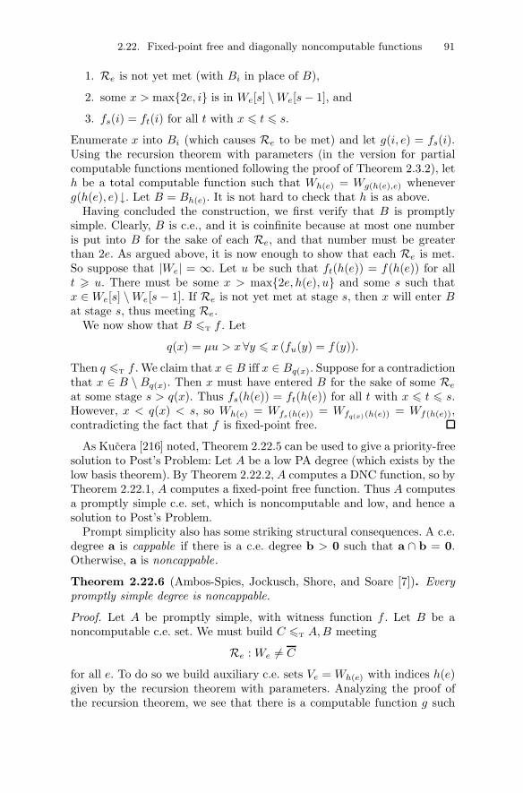
2.22. Fixed-point free and diagonally noncomputable functions 91
1. Re is not yet met (with Bi in place of B),
2. some x > max{2e, i} is in We[s] \We[s− 1], and
3. fs(i) = ft(i) for all t with x � t � s.
Enumerate x into Bi (which causes Re to be met) and let g(i, e) = fs(i).Using the recursion theorem with parameters (in the version for partialcomputable functions mentioned following the proof of Theorem 2.3.2), leth be a total computable function such that Wh(e) = Wg(h(e),e) wheneverg(h(e), e)↓. Let B = Bh(e). It is not hard to check that h is as above.
Having concluded the construction, we first verify that B is promptlysimple. Clearly, B is c.e., and it is coinfinite because at most one numberis put into B for the sake of each Re, and that number must be greaterthan 2e. As argued above, it is now enough to show that each Re is met.So suppose that |We| = ∞. Let u be such that ft(h(e)) = f(h(e)) for allt � u. There must be some x > max{2e, h(e), u} and some s such thatx ∈ We[s] \We[s− 1]. If Re is not yet met at stage s, then x will enter Bat stage s, thus meeting Re.
We now show that B �T f . Let
q(x) = μu > x∀y � x (fu(y) = f(y)).
Then q �T f . We claim that x ∈ B iff x ∈ Bq(x). Suppose for a contradictionthat x ∈ B \ Bq(x). Then x must have entered B for the sake of some Re
at some stage s > q(x). Thus fs(h(e)) = ft(h(e)) for all t with x � t � s.However, x < q(x) < s, so Wh(e) = Wfs(h(e)) = Wfq(x)(h(e)) = Wf(h(e)),contradicting the fact that f is fixed-point free.
As Kucera [216] noted, Theorem 2.22.5 can be used to give a priority-freesolution to Post’s Problem: Let A be a low PA degree (which exists by thelow basis theorem). By Theorem 2.22.2, A computes a DNC function, so byTheorem 2.22.1, A computes a fixed-point free function. Thus A computesa promptly simple c.e. set, which is noncomputable and low, and hence asolution to Post’s Problem.
Prompt simplicity also has some striking structural consequences. A c.e.degree a is cappable if there is a c.e. degree b > 0 such that a ∩ b = 0.Otherwise, a is noncappable.
Theorem 2.22.6 (Ambos-Spies, Jockusch, Shore, and Soare [7]). Everypromptly simple degree is noncappable.
Proof. Let A be promptly simple, with witness function f . Let B be anoncomputable c.e. set. We must build C �T A,B meeting
Re : We �= C
for all e. To do so we build auxiliary c.e. sets Ve = Wh(e) with indices h(e)given by the recursion theorem with parameters. Analyzing the proof ofthe recursion theorem, we see that there is a computable function g such

92 2. Computability Theory
that for almost all n, if we decide to put n into Ve at a stage s, then nenters Wh(e) before stage g(s).
Our strategy for meeting Re is straightforward. We pick a follower ntargeted for C. If we ever see a stage s such that n ∈ We,s, we declare nto be active. If We ∩ Cs = ∅, then we pick a new follower n′ > n. For anactive n, if some number less than n enters B at a stage t, we enumeraten into Ve. If n ∈ Af(g(t)) then we put n into C. In any case, we declare nto be inactive.
Assume for a contradiction that We = C. Then infinitely many followersbecome active during the construction. Since B is noncomputable, infinitelymany of these enter Wh(e), so by the prompt simplicity of A, some activefollower enters C, whence We �= C.
The strategies for different requirements act independently, choosing fol-lowers in such a way that no two strategies ever have the same follower.Thus all requirements are met. Whenever we enumerate n into C at a staget, this action is permitted by a change in B below n at stage t and by nitself entering A by stage f(g(t)). Since f is computable, C �T A,B.
Ambos-Spies, Jockusch, Shore, and Soare [7] extended the above resultby showing that the promptly simple degrees and the cappable degreesform an algebraic decomposition of the c.e. degrees into a strong filterand an ideal. (See [7] for definitions.) Furthermore, they showed that thepromptly simple degrees coincide with the low cuppable degrees, where ais low cuppable if there is a low c.e. degree b such that a ∪ b = 0′. Theproofs of these results are technical, and would take us too far afield.
Corollary 2.22.7 (Kucera [216]). Let a and b be Δ02 degrees both of which
compute fixed-point free functions. Then a and b do not form a minimalpair.
Proof. By Theorem 2.22.5, each of a and b bounds a promptly simpledegree. By Theorem 2.22.6, these promptly simple degrees are noncappable,and hence do not form a minimal pair. Thus neither do a and b.20
Kucera [217] introduced the following variation of the notion of DNCfunction.
Definition 2.22.8 (Kucera [217]). A total function f is generallynoncomputable (GNC ) if f(〈e, n〉) �= Φe(n) for all e and n.
We can argue as before to show that the degrees computing {0, 1}-valued GNC functions are exactly the degrees computing {0, 1}-valuedDNC functions, that is, the PA degrees.
20Kucera’s original proof of this result was direct, in the style of the proof of Theorem2.22.5, and used the (double) recursion theorem.

2.23. Array noncomputability and traceability 93
Theorem 2.22.9 (Kucera [217]). Let A be a Π01 class whose elements are
all {0, 1}-valued GNC functions, and let C be a set. There is a functiong ∈ A and an index e such that g(〈e, n〉) = C(n) for all n. Furthermore, ecan be found effectively from an index for A.
Proof. Using the recursion theorem, choose e such that Φe(n) is defined asfollows. Suppose there is a τ ∈ 2<ω such that
A ∩ {f : ∀n < |τ | (f(〈e, n〉) = τ(n))} = ∅.This condition is c.e., so we can choose the first τ we see satisfying it andlet Φe(n) = 1 − τ(n) for n < |τ | and Φe(n) = 0 for n � |τ |. If there is nosuch τ , then let Φe(n)↑ for all n.
If there is such a τ , then for each {0, 1}-valued GNC function f we havef(〈e, n〉) = τ(n) for all n < |τ |, and hence A ∩ {f : ∀n < |τ | (f(〈e, n〉) =τ(n))} = A �= ∅, contradicting the definition of τ . Thus there is no such τ ,and hence for every σ there is a g ∈ A such that g(〈e, n〉) = σ(n) for alln < |σ|. By compactness, there is a g ∈ A such that g(〈e, n〉) = C(n) forall n.
Kucera [217] remarked that the use of 〈e, n〉 with Φe(n)↑ for all n is ananalog of the use of what are known as flexible formulas in axiomatizabletheories, first introduced and studied by Mostowski [283] and Kripke [214],in connection with Godel’s Incompleteness Theorem.
In unpublished work,21 Kucera also noted that the above proof can becombined with the proof of the low basis theorem to show that if c is alow degree then there is a low PA degree a � c. Combining this resultwith Kucera’s priority-free solution to Post’s Problem, we see that for anylow degree c there is a c.e. degree b such that b ∪ c is low. This result isparticularly interesting in light of the fact that Lewis [245] has constructeda minimal (and hence low2) degree c such that b∪c = 0′ for every nonzeroc.e. degree b. Kucera has also used the above method to construct PAdegrees in various jump classes.
2.23 Array noncomputability and traceability
In this section, we discuss the array noncomputable degrees introducedby Downey, Jockusch, and Stob [120, 121]. The original definition of thisclass was in terms of very strong arrays. Recall that a strong array is acomputable collection of pairwise disjoint finite sets {Fn : n ∈ N} (whichrecall means not only that the Fn are uniformly computable, but also thatthe function i → maxFi is computable).
21This work is now mentioned as example 2.1 in Kucera and Slaman [222]. In unpub-lished work, Kucera and Slaman have also shown that there is a low2 degree that joinsall Δ0
2 fixed-point free degrees to 0′.

94 2. Computability Theory
Definition 2.23.1 (Downey, Jockusch, and Stob [120]).
(i) A strong array {Fn : n ∈ N} is a very strong array if |Fn| > |Fm| forall n > m.
(ii) For a very strong array F = {Fn : n ∈ N}, we say that a c.e. set A isF-array noncomputable (F-a.n.c.) if for each c.e. set W there is a ksuch that W ∩ Fk = A ∩ Fk.
Notice that for any c.e. set W and any k there is a c.e. set W such thatW ∩ Fk �= W ∩ Fk but W (n) = W (n) for n /∈ Fk. From this observationit follows that if A is F -a.n.c. then for each c.e. set W there are infinitelymany k such that W ∩ Fk = A ∩ Fk.
This definition was designed to capture a certain kind of multiple per-mitting construction. The intuition is that for A to be F -a.n.c., A needs|Fk| many permissions to agree with W on Fk. As we will see below,up to degree, the choice of very strong array does not matter. Downey,Jockusch, and Stob [120] used multiple permitting to show that severalproperties are equivalent to array noncomputability. For example, the a.n.c.c.e. degrees are precisely those that bound c.e. sets A1, A2, B1, B2 such thatA1∩A2 = B1∩B2 = ∅ and every separating set for A1, A2 is Turing incom-parable with every separating set for B1, B2. (There are a number of othercharacterizations of the array noncomputable c.e. degrees in [120, 121].)We will see two examples of this technique connected with algorithmicrandomness in Theorems 9.14.4 and 9.14.7 below.
In Downey, Jockusch, and Stob [121], a new definition of array noncom-putability was introduced, based on domination properties of functions andnot restricted to c.e. sets.
Definition 2.23.2 (Downey, Jockusch, and Stob [121]). A degree a isarray noncomputable (a.n.c) if for each f �wtt ∅′ there is a function gcomputable in a such that g(n) � f(n) for infinitely many n. Otherwise, ais array computable.
Note that, using this definition, the a.n.c. degrees are clearly closedupwards. The following results give further characterizations of array non-computability. They also show that, for c.e. sets, the two definitions ofarray noncomputability coincide and the first definition is independent ofthe choice of very strong array up to degree. Let m∅′(n) be the least s suchthat ∅′ � n = ∅′s � n.
Theorem 2.23.3 (Downey, Jockusch, and Stob [121]). Let a be a degree,and let {Fn}n∈ω be a very strong array. The following are equivalent.
(i) The degree a is a.n.c.
(ii) There is a function h computable in a such that h(n) � m∅′(n) forinfinitely many n.
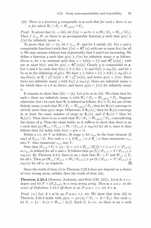
2.23. Array noncomputability and traceability 95
(iii) There is a function g computable in a such that for each e there is ann for which We ∩ Fn = We,g(n) ∩ Fn.
Proof. To prove that (i) → (iii), let f(n) = μs ∀e � n (We∩Fn = We,s∩Fn).Then f �wtt ∅′, so there is an a-computable function g such that g(n) �f(n) for infinitely many n.
To prove that (ii) → (i), let f �wtt ∅′, and let h satisfy (ii). Fix e and acomputable function b such that f(n) = Φ∅′
e (n) with use at most b(n) for alln. We may assume without loss of generality that h and b are increasing. Wedefine a function g such that g(n) � f(n) for infinitely many n as follows.Given n, let s be minimal such that s > h(b(n + 1)) and Φ∅′
e (n)[s] ↓ withuse at most b(n), and let g(n) = Φ∅′
e (n)[s]. Clearly g is computable in a.Let n and k be such that b(n) � k � b(n+ 1) and h(k) � m∅′(k), and let sbe as in the definition of g(n). We have s � h(b(n+1)) � h(k) � m∅′(k) �m∅′(b(n)), so ∅′s � ϕ∅′
e (n)[s] = ∅′ � ϕ∅′e (n)[s], and hence g(n) = f(n). Since
there are infinitely many j with h(j) � m∅′(j), there are infinitely many nfor which there is a k as above, and hence g(n) = f(n) for infinitely manyn.
It remains to show that (iii) → (ii). Let g be as in (iii). We claim that foreach e there are infinitely many n with We ∩ Fn = We,g(n) ∩ Fn. Supposeotherwise. Let i be such that Φi is defined as follows. If x ∈ Fn for one of thefinitely many n such that We∩Fn = We,g(n)∩Fn, then let Φi(x) converge instrictly more than g(n) steps. Otherwise, if Φe(x)↓ then let Φi(x) convergein at least the same number of steps as Φe(x), and if Φe(x) ↑ then letΦi(x)↑. Then there is no n such that Wi∩Fn = Wi,g(n) ∩Fn, contradictingthe choice of g. Thus the claim holds, so it suffices to show that there is ane such that μs (We,s ∩Fn+1 = We ∩Fn+1) � m∅′(n) for all n, since it thenfollows that (ii) holds with h(n) = g(n+ 1).
Define a c.e. set V as follows. At stage s, let cn,s be the least element (ifany) of Fn+1 \ Vs. For each n < s, if ∅′s+1 � n �= ∅′s � n then enumerate cn,sinto V . Also enumerate cs,s into V .
Note that |Fn+1∩V | � |{s : ∃i < n (i ∈ ∅′s+1 \∅′s)}|+1 � n+1 < |Fn+1|,so cn,s is defined for all n and s. It follows that μs (Vs∩Fn+1 = V ∩Fn+1) �m∅′(n). By Theorem 2.3.3, there is an e such that We = V and We,s ⊆ Vsfor all s. Then μs (We,s∩Fn+1 = We∩Fn+1) � μs (Vs∩Fn+1 = V ∩Fn+1) �m∅′(n) for all n, as required.
Since the truth of item (i) in Theorem 2.23.3 does not depend on a choiceof very strong array, neither does the truth of item (iii).
Theorem 2.23.4 (Downey, Jockusch, and Stob [120, 121]). Let a be a c.e.degree and let F = {Fn}n∈N be a very strong array. Then a is a.n.c. in thesense of Definition 2.23.2 iff there is an F-a.n.c. c.e. set A ∈ a.
Proof. (⇐) Let A ∈ a be an F -a.n.c. c.e. set. We show that item (iii) inTheorem 2.23.3 holds with g(n) = μs (As ∩ Fn = A ∩ Fn). For each e,let Ve = {x : ∃s (x ∈ We,s \ As)}. Each Ve is c.e., so there is an n such

96 2. Computability Theory
that A ∩ Fn = Ve ∩ Fn. If x enters We ∩ Fn after stage g(n), then wehave two cases: if x ∈ A then x ∈ Ag(n), so x /∈ Ve, while if x /∈ A thenx ∈ Ve. Both these possibilities contradict the fact that A ∩ Fn = Ve ∩ Fn,so We ∩ Fn = We,g(n) ∩ Fn.
(⇒) Let a be an a.n.c. c.e. degree and let {Fn}n∈N be a very strong array.Let f(n) = μs ∀e � n (We,s ∩ F〈e+1,n〉 = We ∩ F〈e+1,n〉). Clearly f �wtt ∅′,so there is an a-computable g such that g(n) � f(n) for infinitely many n.Since g is a-computable and a is c.e., there is a computable function h(n, s)and an a-computable function p such that g(n) = h(n, s) for all s � p(n).We now define the c.e. set A.
First, we let B ∈ a be c.e. and put⋃n∈B F〈0,n〉 into A. We will not put
any other elements of any F〈0,n〉 into A, so this action ensures that A hasdegree at least a.
Now it suffices to ensure that if n � e and g(n) � f(n), then A ∩F〈e+1,n〉 = We ∩ F〈e+1,n〉. Whenever h(n, s) �= h(n, s + 1) and e � n � s,we put all elements of We,h(n,s+1) ∩ F〈e+1,n〉 into A at stage s.
The definition of A ensures that if x ∈ A∩F〈e+1,n〉 then x ∈ Ap(n), so A iscomputable in p and hence A ∈ a. Suppose now that n � e and g(n) � f(n).It follows from the definition of f that We,g(n) ∩ F〈e+1,n〉 = We ∩ F〈e+1,n〉.Choose s as large as possible so that h(n, s) �= h(n, s + 1). (There is noloss of generality in assuming there is at least one such s � n.) Thenh(n, s+ 1) = g(n) and so
As+1 ∩ F〈e+1,n〉 = We,h(n,s+1) ∩ F〈e+1,n〉= We+1,g(n) ∩ F〈e+1,n〉 = We ∩ F〈e+1,n〉.
Furthermore, by the maximality of s, no elements of F〈e+1,n〉 enter A afterstage s+ 1, so A ∩ F〈e+1,n〉 = We ∩ F〈e+1,n〉.
Corollary 2.23.5 (Downey, Jockusch, and Stob [120, 121]). Let F andG be very strong arrays. Then a degree contains an F-a.n.c. c.e. set iff itcontains a G-a.n.c. c.e. set.
We do not need to consider all wtt-reductions in the definition of arraynoncomputability, but can restrict ourselves to reductions with use boundedby the identity function.
Proposition 2.23.6 (Downey and Hirschfeldt, generalizing [120]). A de-gree a is a.n.c. iff for every f that is computable from ∅′ via a reductionwith use bounded by the identity function, there is an a-computable functiong such that g(n) � f(n) for infinitely many n.
Proof. The “only if” direction is obvious. We prove the “if” direction. Sup-pose that Γ∅′
= f with use bounded by the increasing computable functionp. Let Φ∅′
(n) = max{Γ∅′(m) : p(m) � n}. Then ϕ∅′
(n) � n, so there is ana-computable increasing function g such that g(n) � Φ∅′
(n) for infinitelymany n. Let g(m) = g(p(m+ 1)). Since p is computable, g �T A. Further-

2.23. Array noncomputability and traceability 97
more, if g(n) � Φ∅′(n) then for the largest m such that p(m) � n, we have
g(m) = g(p(m + 1)) > g(n) � Φ∅′(n) � Γ∅′
(m) = f(m), so g(m) � f(m)for infinitely many m.
Martin [258] gave a characterization of the GL2 sets quite close to thedefinition of array computability, as a consequence of the following result.Recall that a function f dominates a function g if f(n) � g(n) for allsufficiently large n. A function is dominant if it dominates all computablefunctions.
Theorem 2.23.7 (Martin [258]). A set A is high iff there is a dominantfunction f �T A.
Proof. Recall that Tot = {e : Φe is total}. This set has degree ∅′′, so Ais high iff Tot �T A′ iff there is an A-computable function h such thatlims h(e, s) = Tot(e) for all e.
Suppose that A is high, and let h be as above. Define an A-computablef as follows. Given n, for each e � n, look for an s � n such that either
1. Φe(n)[s]↓ or
2. h(e, s) = 0.
For each e � n, one of the two must happen. Define f(n) to be larger thanΦe(n) for all e � n such that 1 holds. If Φe is total then h(e, s) = 1 forall sufficiently large s, so f(n) > Φe(n) for all sufficiently large n. Thus fdominates all computable functions.
Now suppose that there is a function f �T A that dominates all com-putable functions. Define h �T A as follows. Given e and s, check whetherΦe(n)[f(s)]↓ for all n � s. If so, let h(e, s) = 1, and otherwise let h(e, s) = 0.If e /∈ Tot then clearly h(e, s) = 0 for all sufficiently large s. If e ∈ Tot ands is sufficiently large then f(s) is greater than the stage by which Φe(n)converges for all n � s, since the latter is a computable function of s. Soh(e, s) = 1 for all sufficiently large s. Thus lims h(e, s) = Tot(e) for alle.
Corollary 2.23.8 (Martin [258]). A set A is GL2 iff there is a functionf �T A⊕ ∅′ that dominates all A-computable functions.
Proof. A set A is GL2 iff (A ⊕ ∅′)′ ≡T A′′ iff A ⊕ ∅′ is high relative to A.
Thus the corollary follows by relativizing Theorem 2.23.7 to A.
By Corollary 2.23.8, if a set A is not GL2 then for each function f �T
A ⊕ ∅′ there is a function g �T A such that g(n) � f(n) for infinitelymany n. Thus if a degree is not GL2 then it is a.n.c. In particular, everyarray computable Δ0
2 degree is low2. In [121], Downey, Jockusch, and Stobdemonstrated that many results previously proved for non-GL2 degreesextend to a.n.c. degrees. However, the a.n.c degrees do not coincide with the

98 2. Computability Theory
non-GL2 degrees, nor do the a.n.c. c.e. degrees coincide with the nonlow2
c.e. degrees.
Theorem 2.23.9 (Downey, Jockusch, and Stob [120]). There is a lowa.n.c. c.e. degree.
Proof. The proof is a straightforward combination of lowness and arraynoncomputability requirements. Let F = {Fn : n ∈ N} be a very strongarray with |Fn| = n+ 1. We build a c.e. set A to satisfy the requirements
Re : ∃n (We ∩ Fn = A ∩ Fn)
and
Ne : ∃∞sΦAe (e)[s]↓ ⇒ ΦAe (e)↓ .
For the sake of Re we simply pick a fresh n to devote to making We∩Fn =A ∩ Fn. We do so in the obvious way: Whenever a new element entersWe ∩ Fn, we put it into A. Such enumerations will happen at most n + 1many times. Each time one happens we initialize the weaker priority N -requirements. Similarly, each time we see a computation ΦAe (e)[s] ↓ weinitialize the weaker priority R-requirements, which now must pick theirn’s to be above the use of this computation. The result follows by the usualfinite injury argument.
On the other hand, an easy modification of Martin’s proofs above showsthat if A is superlow then there is a function wtt-computable in ∅′ thatdominates every A-computable function, and hence A is array computable.
Array computability is also related to hyperimmunity.
Proposition 2.23.10 (Folklore). If a is hyperimmune-free then a is arraycomputable.
Proof. If A is of hyperimmune-free degree then every f �T A is dominatedby some total computable function. It is easy to construct a function g �wtt
∅′ that is a uniform bound for all partial computable functions. (That is,for each e, we have Φe(n) � h(n) for almost all n such that Φe(n) ↓.)Then every function f �T A is dominated by g, and hence A is arraycomputable.
The following concept, closely related to both hyperimmune-freeness andarray computability, is quite useful in the study of algorithmic randomness.
Definition 2.23.11 (Zambella [416], see [386], also Ishmukhametov [184]).A set A, and the degree of A, are c.e. traceable if there is a computablefunction p (called a bound) such that, for each function f �T A, there is acomputable function h (called a trace for f) satisfying, for all n,
(i) |Wh(n)| � p(n) and
(ii) f(n) ∈ Wh(n).

2.23. Array noncomputability and traceability 99
Since one can uniformly enumerate all c.e. traces for a fixed bound p,there is a universal trace with bound p2, say. By a universal trace wemean one that traces each function f �T A on almost all inputs. As thefollowing result shows, the above definition does not change if we replace“there is a computable function p” by “for every unbounded nondecreasingcomputable function p such that p(0) > 0”.
Proposition 2.23.12 (Terwijn and Zambella [389]). Let A be c.e. traceableand let q be an unbounded nondecreasing computable function such thatq(0) > 0. Then A is c.e. traceable with bound q.
Proof. Let A be c.e. traceable with some bound p. Let g �T A. For eachm, let rm be such that q(rm) � p(m+1), and let f(m) = 〈g(0), . . . , g(rm)〉.Let h be as in Definition 2.23.11. Let h be a computable function suchthat Wh(n) is defined as follows. For each m, if rm � n < rm+1, thenenumerate into Wh(n) all the nth coordinates of elements of Wh(m+1). Then|Wh(n)| � |Wh(m+1)| � p(m+ 1) � q(rm) � q(n). Furthermore, g(n) is thenth coordinate of f(m + 1), and f(m + 1) ∈ Wh(m+1), so g(n) ∈ Wh(n).We have not yet defined Wh(n) for n < r0, but since there are only finitelymany such n, we can define Wh(n) = {g(n)} for such n. Then for all n wehave |Wh(n)| � q(n) and g(n) ∈Wh(n), as required.
Ishmukhametov [184] gave the following characterization of the arraycomputable c.e. degrees.
Theorem 2.23.13 (Ishmukhametov [184]). A c.e. degree is array com-putable iff it is c.e. traceable.
Proof. Let A be a c.e. traceable c.e. set. Let f �T A. Let p and h be asin Definition 2.23.11. Let g(n) = maxWh(n). Then g �wtt ∅′, since we canuse p(n) to bound the ∅′-oracle queries needed to compute g(n), and gdominates f . Since f is arbitrary, A is array computable.
Now let A be an array computable c.e. set. By Proposition 2.23.6, thereis a function g computable from ∅′ with use bounded by the identity thatdominates every A-computable function. Let f = ΦAe . Let F (n) be theleast s such that ΦAe (n)[t] = ΦAe (n)[s] for all t > s. Then F �T A, soby modifying g at finitely many places, we obtain a function G that iscomputable in ∅′ with use bounded by the identity function and such thatG(n) > F (n) for all n. Since ∅′ � n can change at most n many times duringthe enumeration of ∅′, there is a computable approximation G0, G1, . . .to G that changes value at n at most n times. Let h be a computablefunction such thatWh(n) = {ΦAe (n)[Gs(n)] : s ∈ N∧ΦAe (n)[Gs(n)]↓}. Then|Wh(n)| � n and f(n) ∈ Wh(n). Since f is arbitrary, A is c.e. traceable.
Using this characterization, Ishmukhametov proved the following re-markable theorem, which shows that if the c.e. degrees are definable inthe global structure of the degrees, then so are the a.n.c. c.e. degrees. A

100 2. Computability Theory
degree m is a strong minimal cover of a degree a < m if for all degreesd < m, we have d � a.
Theorem 2.23.14 (Ishmukhametov [184]). A c.e. degree is array com-putable iff it has a strong minimal cover.
Definition 2.23.11 can be strengthened as follows. Recall that D0, D1, . . .is a canonical listing of finite sets, as defined in Chapter 1.
Definition 2.23.15 (Terwijn and Zambella [389]). A set A, and the degreeof A, are computably traceable if there is a computable function p such that,for each function f �T A, there is a computable function h satisfying, forall n,
(i) |Dh(n)| � p(n) and
(ii) f(n) ∈ Dh(n).
As with c.e. traceability, the above definition does not change if wereplace “there is a computable function p” by “for every unboundednondecreasing computable function p such that p(0) > 0”.
If A is computably traceable then each function g �T A is dominatedby the function f(n) = maxDh(n), where h is a trace for f . Thus, everycomputably traceable degree is hyperimmune-free. One may think of com-putable traceability as a uniform version of hyperimmune-freeness. Terwijnand Zambella [389] showed that a simple variation of the standard con-struction of hyperimmune-free sets by Miller and Martin [282] (Theorem2.17.3) produces continuum many computably traceable sets. Indeed, theproof we gave of Theorem 2.17.3 produces a computably traceable set.
2.24 Genericity and weak genericity
The notion of genericity arose in the context of set-theoretic forcing. It wassubsequently “miniaturized” to obtain a notion of n-genericity appropriateto computability theory. Although the original definition of n-genericitywas in terms of forcing, the following more modern definition is the onethat is now generally used.22 Let S ⊆ 2<ω. A set A meets S if there is an
22The original definition of n-genericity, dating back to Feferman [143], is as follows.Let L be the usual first-order language of number theory together with a set constantX and the membership relation ∈. Let σ ∈ 2<ω . For sentences ψ in L, we define thenotion “σ forces ϕ”, written σ � ψ, by recursion on the structure of ψ as follows.
(i) If ψ is atomic and does not contain X, then σ � ψ iff ψ is true in arithmetic.
(ii) σ � n ∈ X iff σ(n) = 1.
(iii) σ � ψ0 ∨ ψ1 iff σ � ψ0 or σ � ψ1.
(iv) σ � ¬ψ iff ∀τ � σ (τ �� ψ).
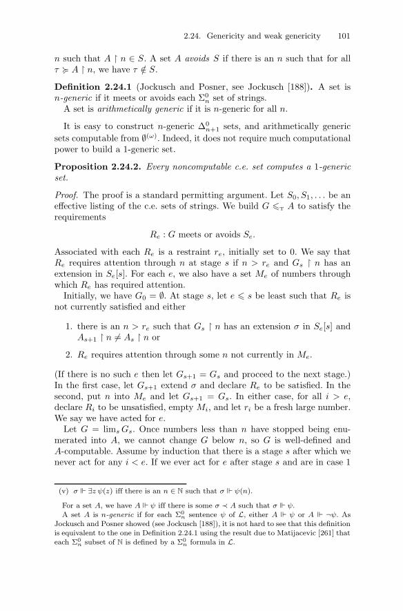
2.24. Genericity and weak genericity 101
n such that A � n ∈ S. A set A avoids S if there is an n such that for allτ � A � n, we have τ /∈ S.
Definition 2.24.1 (Jockusch and Posner, see Jockusch [188]). A set isn-generic if it meets or avoids each Σ0
n set of strings.A set is arithmetically generic if it is n-generic for all n.
It is easy to construct n-generic Δ0n+1 sets, and arithmetically generic
sets computable from ∅(ω). Indeed, it does not require much computationalpower to build a 1-generic set.
Proposition 2.24.2. Every noncomputable c.e. set computes a 1-genericset.
Proof. The proof is a standard permitting argument. Let S0, S1, . . . be aneffective listing of the c.e. sets of strings. We build G �T A to satisfy therequirements
Re : G meets or avoids Se.
Associated with each Re is a restraint re, initially set to 0. We say thatRe requires attention through n at stage s if n > re and Gs � n has anextension in Se[s]. For each e, we also have a set Me of numbers throughwhich Re has required attention.
Initially, we have G0 = ∅. At stage s, let e � s be least such that Re isnot currently satisfied and either
1. there is an n > re such that Gs � n has an extension σ in Se[s] andAs+1 � n �= As � n or
2. Re requires attention through some n not currently in Me.
(If there is no such e then let Gs+1 = Gs and proceed to the next stage.)In the first case, let Gs+1 extend σ and declare Re to be satisfied. In thesecond, put n into Me and let Gs+1 = Gs. In either case, for all i > e,declare Ri to be unsatisfied, empty Mi, and let ri be a fresh large number.We say we have acted for e.
Let G = limsGs. Once numbers less than n have stopped being enu-merated into A, we cannot change G below n, so G is well-defined andA-computable. Assume by induction that there is a stage s after which wenever act for any i < e. If we ever act for e after stage s and are in case 1
(v) σ � ∃z ψ(z) iff there is an n ∈ N such that σ � ψ(n).
For a set A, we have A � ψ iff there is some σ ≺ A such that σ � ψ.A set A is n-generic if for each Σ0
n sentence ψ of L, either A � ψ or A � ¬ψ. AsJockusch and Posner showed (see Jockusch [188]), it is not hard to see that this definitionis equivalent to the one in Definition 2.24.1 using the result due to Matijacevic [261] thateach Σ0
n subset of N is defined by a Σ0n formula in L.
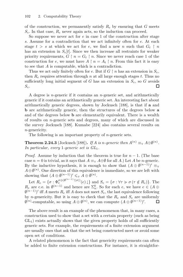
102 2. Computability Theory
of the construction, we permanently satisfy Re by ensuring that G meetsSe. In that case, Re never again acts, so the induction can proceed.
So suppose we never act for e in case 1 of the construction after stages. Assume for a contradiction that we act infinitely often for e. At eachstage t > s at which we act for e, we find a new n such that Gt � nhas an extension in Se[t]. Since we then increase all restraints for weakerpriority requirements, G � n = Gt � n. Since we never reach case 1 of theconstruction for e, we must have A � n = At � n. From this fact it is easyto see that A is computable, which is a contradiction.
Thus we act only finitely often for e. But if G � n has an extension in Se,then Re requires attention through n at all large enough stages t. Thus nosufficiently long initial segment of G has an extension in Se, so G avoidsSe.
A degree is n-generic if it contains an n-generic set, and arithmeticallygeneric if it contains an arithmetically generic set. An interesting fact aboutarithmetically generic degrees, shown by Jockusch [188], is that if a andb are arithmetically generic, then the structures of the degrees below aand of the degrees below b are elementarily equivalent. There is a wealthof results on n-generic sets and degrees, many of which are discussed inthe survey Jockusch [188]. Kumabe [224] also contains several results onn-genericity.
The following is an important property of n-generic sets.
Theorem 2.24.3 (Jockusch [188]). If A is n-generic then A(n) ≡T A⊕∅(n).In particular, every 1-generic set is GL1.
Proof. Assume by induction that the theorem is true for n− 1. (The basecase n = 0 is trivial, as it says that A ≡T A⊕∅ for all A.) Let A be n-generic.By the inductive hypothesis, it is enough to show that (A ⊕ ∅(n−1))′ ≡T
A⊕∅(n). One direction of this equivalence is immediate, so we are left withshowing that (A⊕ ∅(n−1))′ �T A⊕ ∅(n).
Let Re = {σ : Φσ⊕(∅(n−1)�|σ|)e (e)↓} and Se = {σ : ∀τ � σ (τ /∈ Re)}. The
Re are c.e. in ∅(n−1) and hence are Σ0n. So for each e, we have e ∈ (A ⊕
∅(n−1))′ iff A meets Re iff A does not meet Se, the last equivalence followingby n-genericity. But it is easy to check that the Re and Se are uniformly∅(n)-computable, so using A⊕ ∅(n), we can compute (A⊕ ∅(n−1))′.
The above result is an example of the phenomenon that, in many cases, aconstruction used to show that a set with a certain property (such as beingGL1) exists actually shows that the given property holds of all sufficientlygeneric sets. For example, the requirements of a finite extension argumentare usually ones that ask that the set being constructed meet or avoid someopen set of conditions.
A related phenomenon is the fact that genericity requirements can oftenbe added to finite extension constructions. For instance, it is straightfor-

2.24. Genericity and weak genericity 103
ward to modify the construction in the proof of Theorem 2.16.2 to obtainthe following result.
Theorem 2.24.4. If C > 0 and D �T ∅′ ⊕C then there is a 1-generic setA such that A′ ≡T A⊕ C ≡T D.
The following result exemplifies the fact that generic sets are quitecomputationally weak.
Theorem 2.24.5 (Demuth and Kucera [96]). If a set is 1-generic then itdoes not compute a DNC function.
Proof. Let G be 1-generic and let ΦG = f . Let
S = {σ ∈ ω<ω : ∀n < |σ| (σ(n) �= Φn(n))}.
Note that S is co-c.e. Let
X = {τ : ∃σ (Φτ � |σ|↓= σ ∧ σ /∈ S)}.
Then X is c.e., so G either meets or avoids X . If G meets X then there isa τ ≺ G and a σ ∈ ω<ω such that Φτ � |σ| ↓= σ and σ /∈ S. Since ΦG = f ,we have σ ≺ f , and hence f is not DNC. Thus it is enough to assume thatG avoids X and derive a contradiction.
Let ν ≺ G be such that if τ ∈ X then ν ⊀ τ . Let
Y = {σ : ∃ρ (ν ≺ ρ ∧ Φρ � |σ|↓= σ)}.
Then Y is a c.e. subset of S, and it is infinite because every initial segmentof f is in Y . So we can computably find σ0, σ1, . . . ∈ S such that |σi| > i.Let g(i) = σi(i). Then g is computable and, by the definition of S, it isDNC, which is a contradiction.
By Theorem 2.22.2, we have the following result.
Corollary 2.24.6. No PA degree is computable from a 1-generic degree.
Since the hyperimmune-free basis theorem implies that there is a DNCfunction of hyperimmune-free degree, we have the following.
Corollary 2.24.7 (Downey and Yu [137]). There is a hyperimmune-freedegree not computable from any 1-generic degree.
Corollary 2.24.7 should be contrasted with the following result, whoseproof uses a special notion of perfect set forcing.
Theorem 2.24.8 (Downey and Yu [137]). There is a hyperimmune-freedegree computable from a 1-generic degree.
Recall that a set A is CEA if it is computably enumerable in some X <T
A. By Theorem 2.17.2, no set of hyperimmune-free degree can be CEA.There are also noncomputable Δ0
2 sets that are not CEA. For example, letA be co-c.e. If A is c.e. in X , then A is computable in X , so A is not CEA.
104 2. Computability Theory
The following result will be of interest in Section 8.21.3, where we show thatbeing CEA is in fact a property of almost all sets, in the measure-theoreticsense.
Theorem 2.24.9 (Jockusch [188]). Every 1-generic set is CEA.
Proof. 23 Let A be 1-generic. Let X = {2〈i, j〉 : i ∈ A ∧ 2〈i, j〉 /∈ A}.Clearly, X �T A. For each i, the set {σ : ∃j (σ(2〈i, j〉) = 0)} is computableand dense, so for each i there is a j such that 2〈i, j〉 /∈ A. Thus i ∈ A iff∃j (2〈i, j〉 ∈ X), whence A is c.e. in X . So A is CEA(X), and thus we areleft with showing that A �T X .
Let σ be the unique string of length |σ| such that σ(n) = 1 iff n = 2〈i, j〉for i and j such that σ(i) = 1 and σ(2〈i, j〉) = 0. We claim that if ν � σand n � |ν| is odd, then there is a string τ � ν such that τ(n) = 1 andσ � τ .
If σ(n) = 1 then we can take τ = σ, and if n � |σ| then we can take anyτ � σ such that τ(n) = 1. So suppose that σ(n) = 0. Let S be the smallestset under inclusion such that n ∈ S, and if i ∈ S, then 2〈i, j〉 ∈ S if σ(i) = 0and 2〈i, j〉 < |σ|. Let τ be the string of length |σ| such that τ(k) = 1 iffeither σ(k) = 1 or k ∈ S. Then ν � τ . We need to show that σ � τ . Letk � |σ|. If k is odd then σ(k) = τ (k) = 0, so assume that k = 2〈i, j〉 forsome i and j.
If σ(k) = 0, then either σ(i) = 0 or σ(2〈i, j〉) = 1. In the latter case,τ(2〈i, j〉) = 1, so τ(2〈i, j〉) = 0. Now suppose that σ(i) = 0. If i ∈ S,then 2〈i, j〉 ∈ S, so τ(2〈i, j〉) = 1, and hence τ (2〈i, j〉) = 0. If i /∈ S, thenτ(i) = 0 and hence τ(2〈i, j〉) = 0.
If σ(k) = 1, then σ(i) = 1 and σ(2〈i, j〉) = 0. Since σ(i) = 1, we haveτ(i) = 1. Furthermore, it follows easily by induction that S contains nonumbers of the form 2〈d, q〉 with σ(d) = 1. Since σ(2〈i, j〉) = 0 and 2〈i, j〉 /∈S, we have τ(2〈i, j〉) = 0, and hence τ(k) = 1.
We have established our claim. Now assume for a contradiction thatΦX = A for some Turing functional Φ. Let V = {σ : σ | Φσ}. Then Vis c.e. and A extends no string in V , so, since A is 1-generic, there is aν ≺ A such that no extension of ν is in V . Let n � |ν| and σ � ν be suchthat n is odd and Φσ(n) = 0. (Such a σ must exist because {ρ : ∃n �|ν| (n odd ∧ ρ(n) = 0)} is computable and dense, so there is an odd n � |ν|such that ΦX(n) = A(n) = 0.) Then there is a τ � ν such that τ(n) = 1and σ � τ . We have Φτ (n) = 0 and τ(n) = 1, so τ ∈ V , contradicting thechoice of ν.
We now consider a weaker notion of genericity. A set of stringsD is denseif every string has an extension in D. Recall that a set A meets D if thereis a σ ∈ D such that σ ≺ A. Similarly, a string τ meets D if there is a
23Jockusch [188] attributes the idea behind this proof to Martin.

2.24. Genericity and weak genericity 105
σ ∈ D such that σ � τ . Given the set-theoretic definition of genericity interms of meeting dense sets, the following definition is natural.
Definition 2.24.10 (Kurtz [228, 229]). A set is weakly n-generic if it meetsall dense Σ0
n sets of strings. A degree is weakly n-generic if it contains aweakly n-generic set.
As noted by Jockusch (see [228, 229]), it is not hard to show that A isweakly (n+1)-generic iff A meets all dense Δ0
n+1 sets of strings iff A meetsall dense Π0
n sets of strings.Clearly, if a set is n-generic then it is weakly n-generic. The following
result is slightly less obvious.
Theorem 2.24.11 (Kurtz [228, 229]). Every weakly (n+ 1)-generic set isn-generic.
Proof. Let A be weakly (n + 1)-generic. Let S be a Σ0n set of strings. Let
R = {σ : σ ∈ S ∨ ∀τ � σ (τ /∈ S)}. Then R is a dense Σ0n+1 set of strings,
and hence A meets R, which clearly implies that A meets or avoids S. ThusA is n-generic.
Thus we have the following hierarchy: weakly 1-generic ⇐ 1-generic ⇐weakly 2-generic ⇐ 2-generic ⇐ weakly 3-generic ⇐ · · · . We now show thatnone of these implications can be reversed, even for degrees, by exploringthe connection between weak genericity and hyperimmunity. Recall that adegree a is hyperimmune relative to a degree b if there is an a-computablefunction that is not majorized by any b-computable function.
Theorem 2.24.12 (Kurtz [228, 229]). If A is weakly (n+1)-generic, thenthe degree of A is hyperimmune relative to 0(n).
Proof. Let pA be the principal function of A. (That is, pA(n) is the nthelement of A in the natural order.) We show that no 0(n)-computable func-tion majorizes pA. Let f be a 0(n)-computable function. For a string σ, letpσ be the principal function of {n < |σ| : σ(n) = 1} (which is a partialfunction, of course). Let Sf = {σ : ∃n (pσ(n)↓> f(n))}. Then Sf is a denseΔ0n+1 set, so A meets Sf , and hence f does not majorize pA.
Corollary 2.24.13 (Kurtz [228, 229]). There is an n-generic degree thatis not weakly (n+ 1)-generic.
Proof. There is an n-generic degree that is below 0(n), and hence nothyperimmune relative to 0(n).
Theorem 2.24.14 (Kurtz [228, 229]). A degree b is the nth jump of aweakly (n + 1)-generic degree iff b > 0(n) and b is hyperimmune relativeto 0(n).
Proof. Suppose that b = a(n) with a weakly (n + 1)-generic. By Theo-rem 2.24.12, a is hyperimmune relative to 0(n), and the class of degrees

106 2. Computability Theory
that are hyperimmune relative to 0(n) is clearly closed upwards. Thus b ishyperimmune relative to 0(n). Clearly, b � 0(n), so in fact b > 0(n).
The proof of the converse is a variant of the proof of the FriedbergCompleteness Criterion (Theorem 2.16.1). Let b > 0(n) be hyperimmunewith respect to 0(n). Let h be a b-computable function that is not majorizedby any 0(n)-computable function. We may assume that h is increasing andhas degree exactly b, and let B = rng h, so that h = pB and deg(B) = b.Let f0, f1, . . . be uniformly 0(n)-computable functions such that {rng fi :i ∈ N} is the collection of all nonempty Σ0
n+1 sets of strings. Let Si = rng fiand let Ssi = {σ : ∃k � pB(s) (fi(k) = σ)}.
We build a set A by finite extensions σ0 � σ1 � · · · so that A(n) ≡T Band A is weakly (n+ 1)-generic. We meet the requirements
Re : If Se is dense then A meets Se.
We say that Re requires attention at stage s if σs does not meet Sse , butthere is a string τ � σs01e+10 that meets Sse . Our construction is donerelative to B, which can compute ∅(n), and hence we can test whether agiven requirement requires attention at a given stage.
The peculiar form that τ must have comes from the coding of B intoA(n). The number e encodes which requirement is being addressed, whichwill allow us to “unwind” the construction to recover the coding. We willsay that a stage s is a coding stage if we act to code information about Binto A at stage s. Let c(s) denote the number of coding stages before s.
At stage 0, declare that 0 is a coding stage and let σ0 = B(0).At stage s + 1, if no requirement Re with e � s + 1 requires attention
then let σs+1 = σs and declare that s+ 1 is not a coding stage. Otherwise,let Re be the strongest priority requirement requiring attention. Let m0
be the least m such that fe(m) � σs01e+10. If |fe(m0)| > s + 1, then letσs+1 = σs and declare that s + 1 is not a coding stage. Otherwise, letσs+1 = fe(m0)�B(c(s+ 1)) and declare that s+ 1 is a coding stage.
Let A =⋃s σs.
Lemma 2.24.15. Re requires attention only finitely often.
Proof. Assume by induction that there is a stage s after which no require-ment stronger than Re requires attention. Suppose Re requires attentionat a stage t+1 > s, and let m0 be the least m such that fe(m) � σt01e+10.If |fe(m0)| � s + 1 then Re is met at stage t + 1 and hence never againrequires attention. Otherwise, Re continues to be the strongest priority re-quirement requiring attention until stage |fe(m0)| − 1, at which point it ismet, and never again requires attention.
Lemma 2.24.16. A is weakly (n+ 1)-generic.
Proof. Assume that Se is dense. Let g(s) be the least k such that for eachσ ∈ 2�s+1 there is a j � k such that fe(j) extends σ01e+10. Then g �T ∅(n).Let s be a stage after which no requirement stronger than Re ever requires
2.24. Genericity and weak genericity 107
attention. Since pB is not majorized by any ∅(n)-computable function, thereis a t > s such that pB(t) > g(t). At stage t, the requirement Re requiresattention unless it is already met, and continues to be the strongest priorityrequirement requiring attention from that stage on until it is met.
Lemma 2.24.17. A(n) �T B.
Proof. Since ∅(n) �T B, the construction of A is computable from B. Bythe previous lemma, A is weakly (n+1)-generic and hence n-generic, so byTheorem 2.24.3, A(n) ≡T A⊕ ∅(n) �T A⊕B ≡T B.
Lemma 2.24.18. B �T A(n).
Proof. Note that A is infinite, as it is weakly (n + 1)-generic. Elementsare added to A only during coding stages, and there are thus infinitelymany such stages s0 < s1 < · · · . During stage sk we define σsk
so thatσsk
(|σsk| − 1) = B(k). Thus it is enough to show that the function g
defined by g(k) = |σsk| is computable from A(n).
We have g(0) = 1. Assume that we have computed g(k) using A(n). Weknow that σsk+1 � σsk
01e+10 for some e, and we can determine this efrom A, since (A � g(k))�01e+10 ≺ A. Since ∅(n) � A(n), we can computefrom A(n) the least m such that fe(m) � σsk
01e+10, which must exist. Byconstruction, g(k + 1) = |fe(m)| + 1.
Together, the three previous lemmas imply the theorem.
Taking n = 0 in the theorem above, we have the following special case,which will be useful below.
Corollary 2.24.19 (Kurtz [228, 229]). A degree is weakly 1-generic iff itis hyperimmune.
Corollary 2.24.20 (Kurtz [228, 229]). There is a weakly (n+ 1)-genericdegree that is not (n+ 1)-generic.
Proof. By the theorem, there is a weakly (n + 1)-generic degree a suchthat a(n) = 0(n+1), so that a(n+1) = 0(n+2). Since a < 0(n+1), we havea(n+1) > a ∨ 0(n+1), so by Theorem 2.24.3, a is not 1-generic.
Downey, Jockusch, and Stob [121] introduced a new notion of genericityrelated to array computability. Let f �pb C mean that f can be computedfrom oracle C by a reduction procedure with a primitive recursive bound onthe use function. It is easy to show that f �pb ∅′ iff there is a computablefunction f(n, s) and a primitive recursive function p such that lims f(n, s) =f(n) and |{s : f(n, s) �= f(n, s + 1)}| � p(n). Most proofs yielding resultsabout array noncomputable degrees that use functions f �wtt ∅′ actuallyuse functions f �pb ∅′.
108 2. Computability Theory
Definition 2.24.21 (Downey, Jockusch, and Stob [121]). (i) A set ofstrings S is pb-dense if there is a function f �pb ∅′ such that f(σ) � σand f(σ) ∈ S for all σ.
(ii) A set is pb-generic if it meets every pb-dense set of strings. A degreeis pb-generic if it contains a pb-generic set.
For every e, the set {σ : σ ∈ We ∨ ∀τ � σ (τ /∈ We)} is pb-dense, soevery pb-generic set is 1-generic. If f �pb ∅′, then the range of f is Σ0
2, soevery 2-generic set is pb-generic.
The main result about pb-genericity of relevance to us is the following.
Theorem 2.24.22 (Downey, Jockusch, and Stob [121]).
(i) If a is a.n.c., then there is a pb-generic set A �T a.
(ii) If A is pb-generic, then deg(A) is a.n.c.
To prove this theorem, we need a lemma. A sequence {Sn}n∈ω of setsof strings is uniformly wtt-dense if there is a function d �wtt ∅′ such thatd(n, σ) � σ and d(n, σ) ∈ Sn for all n and σ.
Lemma 2.24.23 (Downey, Jockusch, and Stob [121]). If a is a.n.c. and{Sn}n∈ω is uniformly wtt-dense, then there is an A �T a that meets eachSn.
Proof. Let d(n, σ) witness the uniform wtt-density of the Sn. Let d andb be computable functions such that lims d(n, σ, s) = d(n, σ) and |{s :d(n, σ, s) �= d(n, σ, s + 1)}| � b(n, σ). We may assume that d(n, σ, s) � σ
for all σ, n, and s. Let h(n, σ) = μs ∀t � s (d(n, σ, t) = d(n, σ, s)). Letf(n) = max{h(e, σ) : e, |σ| � n}. We have f �wtt ∅′, since d �wtt ∅′. Fix afunction g computable in a such that g(n) � f(n) for infinitely many n.
We obtain A as⋃s σs, where |σs| = s. The basic strategy for n at
a stage s > n is to let σt = d(n, σs, g(s)) � t for all t such thats < t � |d(n, σs, g(s))|, at which point we declare Sn to be satisfied.If at any stage u > s we find that for some t ∈ (g(s), g(u)], we haved(n, σs, t) �= d(n, σs, g(s)), then we declare Sn to be unsatisfied and repeatthe strategy. This strategy can be interrupted at any point by the strat-egy for an Sm with m < n. If this situation happens, we wait until Sm issatisfied and repeat the strategy.
Clearly, A �T a, and if Sn is eventually permanently satisfied, then Ameets Sn. To see that every Sn is indeed eventually permanently satisfied,assume by induction that there is a least stage s0 > n by which all Sm withm < n are permanently satisfied. Let s > s0 be such that g(s) � f(s). If aniteration of the strategy for Sn begins at stage s, then it will clearly leadto Sn becoming permanently satisfied. Otherwise, there must be a stagev ∈ [s0, s) such that a strategy for Sn is started at stage v and for all t ∈

2.24. Genericity and weak genericity 109
(g(v), g(s)], we have d(n, σv, t) = d(n, σv, g(v)). But then g(v) � h(n, σv),so Sn is again permanently satisfied.
Proof of Theorem 2.24.22. (i) Let p0, p1, . . . be a uniformly computablelisting of the primitive recursive functions. If Φ∅′
e (m) ↓ with use atmost pi(m) for all m � n, then let g(e, i, n) = Φ∅′
e (n). Otherwise, letg(e, i, n) = 0. Clearly, g �wtt ∅′ and each function f �pb ∅′ has the formn → g(e, i, n) for some e and i. Let σ0, σ1, . . . be an effective listing of 2<ω.Let h(e, i, n) = g(e, i, n) if σg(e,i,n) ⊇ σn, and otherwise let h(e, i, n) = n.Let Se,i = {σh(e,i,n) : n ∈ N}. Then the sets Se,i are uniformly wtt-dense,and every pb-dense set is equal to Se,i for some e and i. By Lemma 2.24.23,there is a set A computable in a that meets each Se,i, which makes Apb-generic.
(ii) Let A = {a0 < a1 < · · · } be pb-generic. Recall that the principalfunction pA of A is defined by pA(n) = an, and that m∅′(n) is the least ssuch that ∅′ � n = ∅′s � n. We show that pA(n) � m∅′(n) for infinitely manyn, which by Theorem 2.23.3 suffices to conclude that deg(A) is a.n.c. For astring σ, let i0 < i1 < · · · < ijσ−1 be all the numbers such that σ(in) = 1.Let pσ(n) = in if n < jσ and let pσ(n) ↑ otherwise. Fix k. We show thatthere is an n � k such that pA(n) � m∅′(n). Let
S = {σ : ∃n � k (pσ(n) � m∅′(n))}.Then S is pb-dense, as witnessed by the function f defined by f(σ) =σ1k0m∅′(jσ+k)1. Thus A meets S, which means that there is a σ such thatf(σ) ≺ A. Then pA(jσ + k) � m∅′(jσ + k).
Since each nonzero c.e. degree bounds a 1-generic degree, but no 2-genericdegree is below 0′, pb-genericity is an intermediate notion between 1- and2-genericity.
Corollary 2.24.24 (Downey, Jockusch, and Stob [121]). There is a 1-generic degree that is not pb-generic, and a pb-generic degree that is not2-generic.
http://www.springer.com/978-0-387-95567-4