computation in the lawrence physics curriculum (17 december
TRANSCRIPT

COMPUTATION IN THE
LAWRENCE PHYSICS
CURRICULUMA Report to the National Science Foundation,
the W. M. Keck Foundation, and Departments of Physics
on Twenty Years of Curricular Development at Lawrence University
DAVID M. COOK
Department of PhysicsLawrence University
Box 599Appleton, Wisconsin 54912

Copyright c© 2006 by David M. Cook
All rights reserved. No part of this document may be re-produced in any form or by any means without permissionin writing from David M. Cook.

Executive Summary
With support from the National Science Foundation, the W. M. Keck Foundation, and LawrenceUniversity, we in the Department of Physics at Lawrence University have for two decades beendeveloping the computational dimensions of our curriculum, both at the introductory and at theintermediate and advanced levels. We have equipped our introductory laboratory with computers,assorted sensors, and suitable software; we have built a Computational Physics Laboratory (CPL)that makes a wide spectrum of hardware and software available to students; we have developed acurricular approach that introduces students to these resources and to prototypical applications;we have incorporated computational dimensions into our advanced laboratory offerings; and wehave drafted several hundred pages of instructional materials, some of which have in the last fewyears been published. This report describes the history of these developments at Lawrence, thecomputational components of our curriculum, and the text written to support these components.
Based on the premise that twenty-first century physicists cannot function fully if they areunaware of the role that computation can play in both theoretical and experimental endeavors andif they lack at least some skill in applying computational approaches when appropriate, we havestructured a curriculum that
• introduces freshmen to computer-based statistical data analysis, curve fitting, graphical visu-alization, and on-line data acquisition,
• requires sophomores to take a course called Computational Mechanics, in which they learnclassical mechanics at an intermediate level, apply symbolic and numerical computation forsolving ordinary differential equations, evaluating integrals, and generating graphical displays,and use LATEX for preparing documents,
• expects students to use computational resources on their own initiative during the rest of theirtime at Lawrence (and encourages that use by granting 24/7 access to the CPL);
• directs students to use computational resources in several upper-level courses;• offers an elective junior/senior course that focuses on finite difference and finite element ap-
proaches to partial differential equations; and• supports the use of computers for the conduct of senior independent studies.
By the time of graduation, all physics majors at Lawrence have developed a comfortable familiaritywith computational approaches to problems and some have become quite adept at sophisticatedapplications.
Among the outcomes of our two-decade long effort is a text, Computation and ProblemSolving in Undergraduate Physics, which has grown along with our curriculum but has also expandedbeyond our curriculum to include, as options, use of software packages different from those chosen atLawrence. This book is now available in several different versions to support inclusion of computationin undergraduate physics curricula at institutions other than Lawrence.
iii

iv EXECUTIVE SUMMARY

Preface and Acknowledgments
The primary purpose of an undergraduate program in physics is to generate a full realization of thebeauty, breadth, and power of the discipline and to develop both an understanding of fundamentalconcepts and the skills to use a variety of tools—both theoretical and experimental—to apply and testthose concepts. In the last two or three decades of the twentieth century, computational approachesto addressing both theoretical and experimental problems have taken their place alongside the moretraditional approaches. The twenty-first century physicist unfamiliar with computational approacheslacks skills that are now critical to the successful pursuit of the field.
To be sure, computers have been used in undergraduate programs in departments of physicsat many institutions for quite some time. The overwhelming majority of these applications, however,has focused on introductory courses, in which—typically—students either run instructor-writtenprograms or access web-based resources, both of which are designed to support the teaching of theconcepts of physics. Valuable though uses of computers to support the teaching of physics havebeen and continue to be, the exposure of undergraduate physics majors to computation cannot belimited to those applications. The important objective for physics majors at the beginning of thetwenty-first century is not so much to learn how to use programs written by others to reinforcefundamental concepts as to learn how to use whatever tools are appropriate and available to createtheir own computer-based solutions. To this end, contemporary curricula must assure that grad-uates are familiar with the capabilities—and limitations—of available tools, are introduced to anassortment of standard algorithms applied in physical contexts to standard problems and, by thetime of graduation, are able to use computers not only for the learning of physics but even more forthe doing of physics.
In the last few years, computation has indeed begun to find its way into upper-level coursesin computational physics or as an inclusion in individual courses on other topics. Unfortunately,these courses often come along late in the student’s undergraduate program, and students thereforedo not encounter computational approaches early enough for those approaches to become almostsecond-nature by the time of graduation. Further, single courses, wherever they occur during thestudents’ undergraduate days, are decoupled from the rest of the curriculum and typically introduceonly those resources needed for the specific course; they do not foster a broad appreciation of theversatility and scope of computational approaches.
In the last couple of years, a systematic and cooperative effort to explore ways to enhancethe use of computation in upper-level undergraduate physics and to provide materials to supportthat effort has finally begun to emerge. At the 2005 summer meeting of the American Association ofPhysics Teachers (AAPT) in Salt Lake City, UT, for example, Bruce Mason, founder of ComPADRE,Norman Chonacky, editor of Computers in Science and Engineering (CiSE ), and David Winch,Professor of Physics Emeritus at Kalamazoo College, convened an informal crackerbarrel session onthe topic “Building a Physics Computing Community for Undergraduate Education”. The sessionwas attended by key early adopters of computational physics who expressed many varied perspectiveson experiences to date and prospects for the future. With support from CiSE, Robert Fuller,
v
vi PREFACE AND ACKNOWLEDGMENTS
Professor of Physics Emeritus at the University of Nebraska, was commissioned to conduct a surveyof all uses of computation in undergraduate physics programs throughout the country. That surveyproduced baseline national data and led to the identification of invitees for contributions both toa session of invited papers and to a poster session at the 2006 summer meeting of the AAPTin Syracuse, NY. Further, the September/October 2006 (Volume 8, Number 5) issue of CiSE wasdevoted to the theme “Computation in Physics Courses”. It included the results of Professor Fuller’ssurvey, five articles about several approaches (texts based on the invited papers delivered at theSyracuse meeting), and—as a sidebar to Guest Editor Professor Winch’s introduction—abstractsof the seventeen invited posters mounted at the poster session at the same meeting. The postersthemselves are available from links at the CiSE website, specifically
http://opac.ieeecomputersociety.org/opac?year=2006&volume=8&issue=5&acronym=cise
On the eve of the invited sessions at the Syracuse meeting and sponsored by CiSE, a dinner discussionamong a dozen and a half of the current major players launched a collaborative effort to developways to include more computation in undergraduate physics programs. As next steps, CiSE EditorChonacky is spearheading that effort by offering CiSE support to continue the national discussionand by seeking the support of professional societies and outside foundations for a developmentproject. The theme issue of CiSE is an example of publicizing the effort. In November, 2006, theShodor Educational Foundation convened a meeting of selected players to brainstorm about andplan the next steps toward such a project.
The Department of Physics at Lawrence University has been ahead of the pack. In themid 1980s, we recognized the growing importance of computation to the serious physicist. Sincethat time, we have been striving to embed the use of general purpose graphical, symbolic, andnumerical computational tools throughout our curriculum. Developed over more than two decades,our approach involves
• introducing freshman to tools for on-line data acquisition, statistical data analysis and curvefitting;
• introducing sophomores to the simulation of electronic circuits in Electronics,
• introducing sophomores to computer-based symbolic, numerical, and visualization tools in arequired course titled Computational Mechanics, which develops classical mechanics at an inter-mediate level while giving particular attention to uses of computational resources in applicationto mechanics problems that involve graphical visualization, ordinary differential equations, in-tegrals, eigenvalues, and eigenvectors, and to introducing the use of LATEX for the preparationof documents and reports;
• incorporating computational approaches alongside traditional approaches to problems in manyintermediate and advanced courses, most of which list Computational Mechanics as a prereq-uisite;
• providing more exposure to on-line data acquisition, data analysis, graphical visualization ofdata, and report writing in a required junior course titled Advanced Laboratory ;
• offering juniors and seniors the elective course Computational Physics, which has Computa-tional Mechanics as a prerequisite and focuses on numerical solution of the wave, diffusion,and Laplace equations by finite difference and finite element methods.
• making computational resources available and, through 24/7 access to the ComputationalPhysics Laboratory, encouraging students to use these resources routinely on their own initia-tive whenever that use seems appropriate.

PREFACE AND ACKNOWLEDGMENTS vii
In the twenty-plus years since the start of this endeavor, numerous materials have been draftedand redrafted and tested and retested. These materials have now been assembled into a flexibletext that is customizable to reflect many different choices of hardware and software. Details aboutthe Lawrence curricular approach and about this text, titled Computation and Problem Solvingin Undergraduate Physics, are described in this report and also posted on the project web site atwww.lawrence.edu/dept/physics/ccli.
This report, which is being distributed to all domestic departments of physics that offer thebachelor’s degree, embodies a progress report on a project that began slowly at Lawrence Universityin the late 1960s and has been more consciously and vigorously pursued since the mid 1980s. Whilethe project will continue to evolve, it is now sufficiently well developed that documenting its currentstate and some of the underlying motivations seems in order. The author hopes that this reportmay prove useful to the steadily increasing numbers of departments that are giving serious thoughtto including computational physics in their undergraduate curricula. Comments, suggestions, andrequests for additional copies should be directed to the author.
Acknowledgments
I wish here to acknowledge support, encouragement, constructive criticism, andassistance—both financial and otherwise—that have contributed to the evolution of the compu-tational dimensions of the curriculum of the Lawrence University Department of Physics. First, Iam grateful for funding that has come from
• The National Science Foundation:
◦ ILI Grant USE-8851685 for $49433, awarded in June, 1988, for a project entitled “Sci-entific Workstations in Undergraduate Physics”. This grant supported the acquisition ofthe first round of scientific computer workstations at Lawrence and helped to create thefirst Computational Physics Laboratory (CPL).
◦ ILI Grant USE-9052194 for $27455, awarded in June, 1990, for a project titled “TheDiscovery Approach to Undergraduate Introductory Physics”. This grant supported theacquisition of the first round of computers, Vernier interfaces and sensors, and assortedsoftware in the Lawrence introductory physics laboratory and launched the freshmancomponents of the computational inclusions in the Lawrence curriculum.
◦ ILI Grant DUE-9350667 for $48777, awarded in June, 1993, for a project entitled “PartialDifferential Equations in Advanced Undergraduate Physics.” This grant helped to equipthe CPL with the second round of workstations and software to support more elaborateuses for partial differential equations.
◦ ILI Grant DUE-9750580 for $18700, awarded in April, 1997, for a project entitled “Labo-ratory Exercises for a Non-Major Course in the Physics of Music”. This grant provided forthe upgrading of the computers in the Lawrence introductory physics laboratory, mainlyto support the creation of a laboratory to accompany a course in the physics of music,but benefiting the overall introductory program in the Department as well.
◦ CCLI-EMD Grant DUE-9952285 for $177,026, awarded in February, 2000, for a projectentitled “Strengthening Computation in Upper-Level Undergraduate Physics Programs”.This grant supported the final writing of Computation and Problem Solving in Under-graduate Physics (CPSUP) and also, with its supplement (see next item), supported fourweek-long summer faculty workshops that provided constructive feedback on a succes-sion of drafts and enhanced awareness nationally of CPSUP and of the developments atLawrence.

viii PREFACE AND ACKNOWLEDGMENTS
◦ Supplement to CCLI-EMD Grant DUE-9952285 for $3781, awarded in April, 2003, formaking possible the conduct of a fourth workshop in the summer of 2003.
• The W. M. Keck Foundation:
◦ Grant #880969 for $200,000, awarded in June, 1988, for a project entitled “IntegratingScientific Workstations into the Physics Curriculum”. This grant supported the acqui-sition of the first round of scientific workstations at Lawrence, helped to create the firstCPL, and provided funds for summer salaries for Professor Cook and student assistantsto further the curricular development fostered by the acquired hardware.
◦ Grant #931348 for $106,000, awarded in December, 1993, for a project entitled “PreparingPhysics Majors for a Capstone Experience”. This grant supported the enhancementof advanced theoretical, computational, and experimental courses by providing for newequipment, faculty released time for curricular development, summer salaries, and salariesfor student research assistants during summers. (This grant was actually for $250,000,with $144,000 of the total allocated to enhancement of the advanced laboratory.)
◦ Grant #011795 for $140,000, awarded in December, 2001, for a project entitled “ScientificSignature Programs as Vehicles for Departmental Development”. This grant supportedthe enhancement of an already established signature program in computational physics,in particular providing upgraded hardware and also sabbatical support, released time,and student assistants to speed the final development of the two central courses describedin Chapter 4 and the writing of the text for the second of those courses. (This grantwas actually for $400,000, with $260,000 of the total supporting the enhancement of anexisting signature program in laser physics and the creation of a signature program insurface physics.)
• The Alfred P. Sloan Foundation: Grant #B1989-61 for $24000, awarded in December, 1989,for a project entitled “Conference on Using Computational Resources in the Upper-DivisionTheoretical Physics Curriculum”. This grant supported a small conference at Lawrence inJuly, 1990. The objective of the conference was to stimulate thinking among the nineteenparticipants1 about uses of computers in upper-division undergraduate physics. The publishedproceedings were distributed to chairs of all departments offering an undergraduate bachelor’sdegree in physics.
I am also grateful for support from Lawrence University, partly but not solely in the form of matchingfunds for some of the above-listed grants.
Second, I wish to acknowledge the assistance and contributions of 26 Lawrence undergrad-uate physics majors, specifically Peter Strunk, LU ’89, Kristi R. G. Hendrickson, LU ’91, ToddG. Ruskell, LU ’91, Stephen L. Mielke, LU ’92, Ruth Rhodes, LU ’92, Michelle Ruprecht, LU ’92,Sandra Collins, LU ’93, Mark F. Gehrke, LU ’93, Karl J. Geissler, LU ’94, Steven Van Metre, LU ’94,Alain Bellon, LU ’95, Peter Kelly Senecal, LU ’95, Christopher C. Schmidt, LU ’97, Michael D. Sten-ner, LU ’97, Mark Nornberg, LU ’98, Scot Shaw, LU ’98, Jim Truitt, LU ’98, Eric D. Moore, LU ’99,
1In addition to David M. Cook from Lawrence University, participants (with their institutions at the time ofthe conference) were D. Beeman, Harvey Mudd College; Amy L. R. Bug, Swarthmore College; Wolfgang Christian,Davidson College; Robert Ehrlich, George Mason University; Bruce Hawkins, Smith College; William M. MacDonald,University of Maryland; A. John Mallinckrodt, California State Polytechnic University–Pomona; Dawn Meredith,University of New Hampshire; G. W. Parker, North Carolina State University–Raleigh; Desmond N. Penny, SouthernUtah State College; Shafiqur M. Rahman, Allegheny College; Lyle Roelofs, Haverford College; Daniel F. Styer, OberlinCollege; Jan Tobochnik, Kalamazoo College; Pieter Visscher, University of Alabama; Carl Wulfman, University ofthe Pacific; Dean Zollman, Kansas State University; and Paul Zorn, St. Olaf College. Professor Cook’s colleagues atLawrence University and the several students who were research assistants in the summer of 1990 also attended thesessions.

PREFACE AND ACKNOWLEDGMENTS ix
Teresa K. Hayne, LU ’00, Danica Dralus, LU, ’02, Ryan T. Peterson, LU ’03, Scott J. Kaminski,LU ’04, Michelle L. Milne, LU ’04, Lauren E. Kost, LU ’05, Claire Weiss, LU ’07, and Erik Gar-bacik, LU ’08. These students have contributed over the couple of decades past to the evolutionof the use of computational resources in the Lawrence curriculum and the creation of first draftsof numerous instructional pieces to support that evolution. I thank them warmly and sincerely fortheir assistance.
Third, I wish to acknowledge and thank several individuals who have provided reviews ofdrafts or otherwise assisted in the refinement particularly of the major book that has emerged fromthe efforts at Lawrence, including
• numerous students (beyond those specifically named in the previous paragraph) who haveenrolled in my courses over the years and who, directly and indirectly, have made commentsthat have influenced this book.
• my departmental colleagues John R. Brandenberger, Jeffrey A. Collett, Matthew R. Stonek-ing, Paul W. Fontana, and the late J. Bruce Brackenridge, who have listened to my sometimeslengthy observations about matters computational and curricular and offered valuable criti-cisms.
• Wolfgang Christian (Davidson College), Robert Ehrlich (George Mason University), andA. John Mallinckrodt (California State Polytechnic University–Pomona), each of whom par-ticipated in the 1990 Sloan-supported conference on computation in advanced undergraduatephysics and each of whom as a consultant throughout the writing of CPSUP has offered manysuggestions and constructive criticisms.
• the seventy participants2 in the week-long workshops offered at Lawrence in the summers of2001, 2002, and 2003 and who, in that context, provided a critical examination of the evolvingmanuscript and offered numerous suggestions for improvement—in addition to finding manypreviously undetected typographical glitches.
2In July 2001: Steve Adams (Widener University), Russel Kauffman (Muhlenberg College), Marylin Bell (LakeForest College), Lawrence A. Molnar (Calvin College), Thomas R. Greenlee (Bethel College), Elliott Moore (NewMexico Tech), Javier Hasbun (State University of West Georgia), Joelle L. Murray (Linfield College), Derrick Hylton(Spelman College), Paula C. Turner (Kenyon College), Ross Hyman (DePaul University), Scott N. Walck (LebanonValley College), William H. Ingham (James Madison University), and Tim Young (University of North Dakota). InJuly, 2002 (first workshop): Albert Batten (United States Air Force Academy), Andrea Cox LU ’91 (Beloit Col-lege), Brian Cudnik (Prairie View A and M), Craig Gunsul (Whitman College), Kevin Lee (University of Nebraska),Kam-Biu Luk (University of California, Berkeley), Daryl Macomb (Boise State University), Viktor Martisovits (Cen-tral College), Donald Miller (Central Missouri State University), Dorn Peterson (James Madison University), RobertRagan (University of Wisconsin – Lacrosse), Shafiq Rahman (Allegheny College), Rahmathullah Syed (Norwich Uni-versity), Jorge Talamantes (California State University – Bakersfield), Mark Timko (Elmhurst College), Paul Tjossem(Grinnell College), and John Walkup (California Polytechnic Institute – San Luis Obispo). In July, 2002 (second work-shop): Julio Blanco (California State University–Northridge), William Briscoe (George Washington University), PaulBunson (Lawrence University), Albert Chen (Oklahoma Baptist University), K. Kelvin Cheng (Texas Tech Univer-sity), Bob Davis (Taylor University), Mirela Fetea (University of Richmond), David Grumbine (St. Vincent College),Kristi Hendrickson LU ’91 (University of Puget Sound), Tom Herrmann (Eastern Oregon University), Seamus Lagan(Whittier College), Eric Lane (University of Tennessee at Chattanooga), Ernest Ma (Montclair State University),Norris Preyer (College of Charleston), Michael Schillaci (Francis Marion University), Mihir Sejpal (Earlham College),Laura Van Wormer (Hiram College), Mary Lou West (Montclair State University), and Douglas Young (Mercer Uni-versity). In July, 2003: Stephen Addison (University of Central Arkansas), Mohan Aggarwal (Alabama A&M), AnneCaraley (SUNY at Oswego), William Dieterle (California University of Pennsylvania), Timothy Duman (Universityof Indianapolis), Brett Fadem (Colby College), Michael Gray (American University), James Meyer (St. Gregory’sUniversity), Prabasaj Paul (Denison University), David Peterson (Francis Marion University), Edward Pogozelski(SUNY at Geneseo), Chandra Prayaga (University of West Florida), Bruce Richards (Oberlin College), David Seely(Albion College), Adam Smith (Hillsdale College), Walther Spjeldvik (Weber State University), Julie Talbot (StateUniversity of West Georgia), Paul Thomas (University of Wisconsin–Eau Claire), Srinivasa Venugopalan (SUNY atBinghamton), and Alma Zook (Pomona College).

x PREFACE AND ACKNOWLEDGMENTS
• especially Javier Hasbun (State University of West Georgia)—who had students working withalmost the entire manuscript—but also William H. Ingham (James Madison University), Rus-sel Kauffman (Muhlenberg College), Joelle L. Murray (Linfield College), Shafiq Rahman (Al-legheny College), John Thompson (DePaul University), and Tim Young (University of NorthDakota), all of whom used at least portions of the growing manuscript in their teaching dur-ing the academic year 2001–02 and who collectively sent me a wide spectrum of varied andvaluable comments.
Finally (and most important of all), I wish to express deep gratitude for the decades duringwhich my wife, Cynthia, has shown patience, understanding, and support beyond any possibility ofmy ever fully knowing. In truth, I do not know how to thank her.
David M. CookDepartment of PhysicsLawrence UniversityBox 599Appleton, WI 54912
Voice Phone: (920)832-6721FAX: (920)832-6962Email: [email protected]
17 December 2006

Contents
Executive Summary iii
Preface and Acknowledgments v
1 Introduction 1
1.1 Underlying Convictions . . . . . . . . . . . . . . . . . . . . . . . . . . . . . . . . . . . . . 11.2 The Challenge . . . . . . . . . . . . . . . . . . . . . . . . . . . . . . . . . . . . . . . . . . 21.3 Overview of the Lawrence Response . . . . . . . . . . . . . . . . . . . . . . . . . . . . . . 3
2 The Institutional and Departmental Context 5
2.1 About Lawrence . . . . . . . . . . . . . . . . . . . . . . . . . . . . . . . . . . . . . . . . . 52.2 About the Department . . . . . . . . . . . . . . . . . . . . . . . . . . . . . . . . . . . . . 52.3 Signature Programs . . . . . . . . . . . . . . . . . . . . . . . . . . . . . . . . . . . . . . . 72.4 Recruiting of Majors . . . . . . . . . . . . . . . . . . . . . . . . . . . . . . . . . . . . . . 8
3 The Computational Components . . . 11
3.1 Typical Program for Physics Majors . . . . . . . . . . . . . . . . . . . . . . . . . . . . . . 123.2 The Freshman Year (Physics 150, 160) . . . . . . . . . . . . . . . . . . . . . . . . . . . . 133.3 The Sophomore Year . . . . . . . . . . . . . . . . . . . . . . . . . . . . . . . . . . . . . . 16
3.3.1 Electronics (Physics 220) . . . . . . . . . . . . . . . . . . . . . . . . . . . . . . 16
3.3.2 Computational Mechanics (Physics 225) . . . . . . . . . . . . . . . . . . . . . . 17
3.3.3 Electricity and Magnetism (Physics 230) . . . . . . . . . . . . . . . . . . . . . 183.4 The Junior and Senior Years . . . . . . . . . . . . . . . . . . . . . . . . . . . . . . . . . . 18
3.4.1 Quantum Mechanics (Physics 310) . . . . . . . . . . . . . . . . . . . . . . . . . 19
3.4.2 Advanced Laboratory (Physics 330) . . . . . . . . . . . . . . . . . . . . . . . . 19
3.4.3 Computational Physics (Physics 540) . . . . . . . . . . . . . . . . . . . . . . . 20
4 Central Courses 21
4.1 Computational Mechanics (Physics 225) . . . . . . . . . . . . . . . . . . . . . . . . . . . 214.1.1 Outline of the Course . . . . . . . . . . . . . . . . . . . . . . . . . . . . . . . . 224.1.2 Sample Problems from Assignments . . . . . . . . . . . . . . . . . . . . . . . . 234.1.3 Examinations from a Recent Offering . . . . . . . . . . . . . . . . . . . . . . . . 23
4.2 Computational Physics (Physics 540) . . . . . . . . . . . . . . . . . . . . . . . . . . . . . 234.2.1 Outline of the Course . . . . . . . . . . . . . . . . . . . . . . . . . . . . . . . . 244.2.2 The Projects . . . . . . . . . . . . . . . . . . . . . . . . . . . . . . . . . . . . . 26
5 CPSUP 27
5.1 The Challenges . . . . . . . . . . . . . . . . . . . . . . . . . . . . . . . . . . . . . . . . . . 285.2 The Structure of CPSUP . . . . . . . . . . . . . . . . . . . . . . . . . . . . . . . . . . . . 285.3 Potential Uses . . . . . . . . . . . . . . . . . . . . . . . . . . . . . . . . . . . . . . . . . . 305.4 Workshops . . . . . . . . . . . . . . . . . . . . . . . . . . . . . . . . . . . . . . . . . . . . 325.5 Addressing the Publishing Challenge . . . . . . . . . . . . . . . . . . . . . . . . . . . . . 325.6 The Future of CPSUP . . . . . . . . . . . . . . . . . . . . . . . . . . . . . . . . . . . . . 33
xi

xii CONTENTS
A Computational Physics Laboratory 35
A.1 A Brief History . . . . . . . . . . . . . . . . . . . . . . . . . . . . . . . . . . . . . . . . . . 35A.2 Hardware . . . . . . . . . . . . . . . . . . . . . . . . . . . . . . . . . . . . . . . . . . . . . 36A.3 Software . . . . . . . . . . . . . . . . . . . . . . . . . . . . . . . . . . . . . . . . . . . . . . 37A.4 The CPL Library . . . . . . . . . . . . . . . . . . . . . . . . . . . . . . . . . . . . . . . . 37A.5 Network Connections . . . . . . . . . . . . . . . . . . . . . . . . . . . . . . . . . . . . . . 38A.6 Publications about the Project . . . . . . . . . . . . . . . . . . . . . . . . . . . . . . . . 38
A.6.1 Published Books and Papers . . . . . . . . . . . . . . . . . . . . . . . . . . . . . 38A.6.2 Invited Talks and Posters . . . . . . . . . . . . . . . . . . . . . . . . . . . . . . 38A.6.3 Contributed Talks and Posters . . . . . . . . . . . . . . . . . . . . . . . . . . . 39
B Problems from Assignments in Computational Mechanics 41
B.1 Problems from Assignment 1 . . . . . . . . . . . . . . . . . . . . . . . . . . . . . . . . . . 41B.2 Problems from Assignment 2 . . . . . . . . . . . . . . . . . . . . . . . . . . . . . . . . . . 42B.3 Problems from Assignment 3 . . . . . . . . . . . . . . . . . . . . . . . . . . . . . . . . . . 43B.4 Problems from Assignment 4 . . . . . . . . . . . . . . . . . . . . . . . . . . . . . . . . . . 44B.5 Problems from Assignment 5 . . . . . . . . . . . . . . . . . . . . . . . . . . . . . . . . . . 45B.6 Problems from Assignment 6 . . . . . . . . . . . . . . . . . . . . . . . . . . . . . . . . . . 47B.7 Problems from Assignment 7 . . . . . . . . . . . . . . . . . . . . . . . . . . . . . . . . . . 47
C Examinations from Computational Mechanics 49
C.1 Hour Examination #1 – 1 February 2006 . . . . . . . . . . . . . . . . . . . . . . . . . . . 49C.2 Hour Examination #2 – 1 March 2006 . . . . . . . . . . . . . . . . . . . . . . . . . . . . . 52C.3 Final Examination – 15 March 2006 . . . . . . . . . . . . . . . . . . . . . . . . . . . . . . 55
D Options for Projects in Computational Physics 61
D.1 Big Exercise #1 (Assignment 3) . . . . . . . . . . . . . . . . . . . . . . . . . . . . . . . . 62
D.2 Big Exercise #2 (Assignment 6) . . . . . . . . . . . . . . . . . . . . . . . . . . . . . . . . 64
D.3 Big Exercise #3 (Assignment 7) . . . . . . . . . . . . . . . . . . . . . . . . . . . . . . . . 66

Chapter 1
Introduction
1.1 Underlying Convictions
Practicing physicists routinely confront a variety of tasks that support their research but are periph-eral to their main objectives. While physicists in different subareas will probably disagree about therelative importance of particular tasks, most will agree that the more important and most frequentof these tasks involve
• visualizing functions of one, two, and three variables graphically,• solving algebraic equations,• solving ordinary differential equations,• solving partial differential equations,• evaluating integrals,• finding roots, eigenvalues, and eigenvectors,• acquiring data,• displaying data graphically,• performing statistical analyses of data,• fitting theoretically expected functions to data,• processing images, and/or• preparing reports and papers.
More often than not, pursuit of these tasks symbolically and analytically is at best tedious, difficult,and prone to error and at worst essentially impossible. In many cases, however, these tasks canbe addressed by exploiting computational approaches. To facilitate their use of such approaches,practicing physicists of the twenty-first century must be acquainted with1
• a common operating system, preferably some flavor of UNIX or LINUX,• a good text editor, e.g. nedit[1] or xemacs[2],• a spreadsheet program, e.g., Excel [3],• an array/number processor, e.g., IDL[4], MATLAB[5], or OCTAVE[6],• a symbolic manipulator, e.g., MAPLE[7], Mathematica[8], or MAXIMA[9],• a visualization tool, e.g. Kaleidagraph[10] and (IDL, MATLAB, or OCTAVE),
1Citations in square brackets refer to items in the bibliography, which can be found starting on page 69.
1
2 CHAPTER 1. INTRODUCTION
• a standard computational language, e.g., FORTRAN or C or C++, at least sufficient tosupport comfortable use of subroutine packages like Numerical Recipes[11], ODEPACK[12].and MUDPACK[13],
• a program for circuit simulation, e.g., Multisim 7 [14] or SPICE[15];• a program for data acquisition, e.g. LabView [16],• a technical publishing system, e.g., LATEX[17],• a drawing program for creating publication quality figures and diagrams, e.g., Tgif [18], and• a presentation program, e.g., PowerPoint [19].
Undergraduate curricula that do not provide physics majors with at least an orientation to theapplicable algorithms and a reasonable spectrum of the appropriate computational tools are failingto prepare their graduates for the activities that practicing scientists will find themselves doingfrequently and extensively in the twenty-first century.
Beyond the substance of the approaches introduced, a curriculum that responds to theseconvictions must also make sure that students
• are aware of the hazards associated with doing finite-precision arithmetic on floating-pointnumbers.
• are introduced to computational resources early enough so that they can continue to use theseresources at subsequent points in their undergraduate careers, thereby reinforcing the uni-versality and broad applicability of those resources. An upper-level course in computationalphysics is a valuable curricular inclusion, but students need to become acquainted with com-putational resources long before they have either the mathematical or the physical backgroundto profit from a rigorous course in computational physics.
• use computational resources throughout the curriculum, again to emphasize the wide varietyof contexts in which computational resources can be a valuable aid to the conduct of carefulscience. The point is best made—and the skills most reliably developed—if use of theseresources permeates the entire curriculum.
• focus initially on the tools themselves. To be sure, numerous examples drawn from physicalcontexts must be used to motivate the study of techniques and tools, but the focus at firstmust be on the features and capabilities of the tools. Otherwise, knowledge of the tools endsup being limited to the capabilities needed for the specific problems encountered. Simply put,encountering computational tools as an appendix to tasks of higher priority leads to a narrow,unsystematic, and incomplete understanding of the capabilities of the tools and does not fullyset the stage for career-long, confident use of the tools in wider—and possibly unrelated—contexts.
In the broadest of terms, by graduation (and, with any luck well before that time), each studentshould have developed not only the ability to recognize when a computational approach may havemerit but also the skill to pursue that approach confidently, fluently, effectively, knowledgeably, andindependently on his or her own initiative.
1.2 The Challenge
The task before the physics educator is to design a physics curriculum that, without short-changingimportant topics from the historical curriculum, nonetheless includes exposure to and opportunityto build skill in the use of computational approaches to a selected important set of representative

1.3. OVERVIEW OF THE LAWRENCE RESPONSE 3
problems in physics. The skills must, of course, be developed within the context of numerous specificproblems from several areas of physics. The end objective, however, is not so much the results ofthe analyses of those problems as the development of generalizable skills that prepare the student toapply appropriate computational tools to other problems as they arise during the course of a careerand that provide a solid foundation on which the student can readily learn new computationaltechniques as the need arises.
1.3 Overview of the Lawrence Response
The response in the Department of Physics at Lawrence University to the challenge posed in Sec-tion 1.2 involves building infrastructure (i.e., acquiring hardware and software), revising curricula,and drafting instructional materials—all of which contribute to our moving towards a full addressingof the goals laid out in Section 1.1. More specifically, we have
• equipped our introductory and advanced laboratories with appropriate hardware and software—see Sections 3.2 and 3.4.2, respectively—and built a Computational Physics Laboratory(CPL)—see Appendix A.
• introduced computer acquisition of data, statistical analysis of data, and least squares fittingin the introductory laboratories, as described in Section 3.2.
• introduced simulation of electronic circuits in Electronics, as described in Section 3.3.1.
• introduced Computational Mechanics, a required sophomore course that orients majors to theCPL, as described briefly in Section 3.3.2 and more extensively in Section 4.1.
• introduced relaxation methods for Laplace’s equation in Electromagnetic Theory, as describedin Section 3.3.3.
• reinforced techniques for graphical visualization and for numerical and symbolic solution ofordinary differential equations, evaluation of integrals, and finding of eigenvalues and eigen-vectors in Quantum Mechanics, as described in Section 3.4.1.
• expanded the majors’ exposure to on-line data acquisition, techniques for data analysis andcurve fitting, and use of publishing software for generating reports in Advanced Laboratory, asdescribed in Section 3.4.2.
• introduced Computational Physics, an elective junior/senior course that focuses on partialdifferential equations and the graphical visualization of their solutions, as described briefly inSection 3.4.3 and more extensively in Section 4.2.
• incorporated computer-based exercises in other courses, as described at the beginning of Sec-tion 3.4.
• drafted and redrafted numerous documents and, ultimately, a book, as described in Chapter 5.
• sought outside funding. A complete listing of outside support is included in the section titledAcknowledgements on page vii in the preface.
• publicized our efforts in a number of talks, posters, and journal articles. A full listing of theseitems is presented in Appendix A.6.

4 CHAPTER 1. INTRODUCTION
The Lawrence approach to developing the abilities of students to use computational resources isactive; it requires students to play a personal role in their own learning; it forces students to defendtheir work in writing; it gives students practice in preparing and delivering oral presentations; itencourages students to work in groups; and it permeates our curriculum. More than any otherobjective, we encourage students to use our computational resources whenever they feel it appro-priate to do so, and we expect that, by the time of graduation, students will have developed botha secure knowledge of computer-based approaches and the initiative and confidence to exploit thoseapproaches on their own initiative.
In Chapters 3–5, we provide fuller detail on the several computational dimensions of thephysics major at Lawrence. For background, however, we begin in Chapter 2 with a brief descriptionof the broader institutional and departmental context.
Chapter 2
The Institutional andDepartmental Context
2.1 About Lawrence
Founded in 1847 and located in Appleton, Wisconsin, Lawrence University is a nationally ranked,private, coeducational, residential liberal arts college and conservatory of music with 130 full-timefaculty members and 1400 full-time students. Of the students, 1100 are pursuing the bachelor of artsdegree in the college, 165 are pursuing the bachelor of music degree in the conservatory, and 135 arepursuing a five-year program leading to both degrees. About 10% of the students come from countriesother than the United States. A student-faculty ratio of about 11:1 fosters personalized teachingand responsiveness to individual student needs. Small classes, specialized tutorials, and extensivefaculty-student collaboration in research characterize the Lawrence program. Jill Beck is currentlyin her third year as president of Lawrence University, succeeding Richard Warch, who served fortwenty-five years prior to his retirement in June, 2004. For the past several years, applicant pressureat Lawrence has been growing—2315 applicants,1304 admitted students, and an entering freshmanclass of 374 in the fall of 2006. As of 30 June 2006, endowment stood at about $200M. In theacademic year 2000–01, our Departments of Chemistry and Biology moved to a new 78,000 squarefoot, $18.1M science building (which also houses research space for one physics faculty member) and,in the fall of 2001, the Department of Physics moved into substantially renovated spaces enlargedby 40% in Youngchild Hall, which was first occupied in 1963 but experienced a $10M renovationduring the academic year 2000–01.
2.2 About the Department
The Department of Physics at Lawrence consists of five full-time faculty members. Professor DavidM. Cook (Ph.D., Harvard, 1965; joined the faculty in 1965), who works in mathematical and com-putational physics, and Professor John R. Brandenberger (Ph.D., Brown, 1968; joined the facultyin 1968), whose interests lie in experimental atomic physics, laser spectroscopy, and the foundationsof quantum mechanics, will be retiring in June, 2008. Associate Professor Jeffrey A. Collett (Ph.D.,Harvard, 1983; joined the faculty in 1995) is a condensed matter physicist who studies phase transi-tions in thin films of liquid crystals. Associate Professor of Physics Matthew R. Stoneking (Ph.D.,University of Wisconsin, 1994; joined the faculty in 1997) studies non-neutral plasmas. Associate
5

6 CHAPTER 2. THE INSTITUTIONAL AND DEPARTMENTAL CONTEXT
Professor of Physics Megan K. Pickett (Ph.D., Indiana University, 1995; joined the faculty in 2006)is a computational astrophysicist and is Professor Cook’s successor. In addition, Lawrence FellowJoan P. Marler (Ph.D., University of California–San Diego, 2005; joined the faculty in 2005) is a fun-damental particle physicist in the second year of a two-year appointment. Finally, the Departmentbenefits from the services of Mr. LeRoy Frahm, electronics technician, and Mr. Thomas Hesselman,machinist and instrument maker. Searches are currently underway for Professor Brandenberger’ssuccessor and for a Ph.D. physicist to be offered a three-year appointment as a Visiting AssistantProfessor of Physics, a continuing position that was created in 1996 and whose holder changes everytwo or three years. With those hires, the Department will be fully staffed at five FTE in the yearsafter Professors Brandenberger and Cook retire.
In the mid 1980s, the Department of Physics adopted the goal of becoming one of thepremier small undergraduate physics departments in the country. To be sure, if a department is tobe included in that group, the departmental course offerings—its curriculum—must be first rate.We are convinced, however, that a departmental program must be much more than its curriculum.In particular, we strive each year to
• foster out-of-class interactions among students and between students and faculty (twice-weeklymid-afternoon teas, annual department-wide weekend retreat, fall picnic),
• involve students in hosting visitors and candidates for positions,• discuss matters of departmental concern with students,• actively recruit prospective students and involve current students in those efforts,• encourage students to work together,• provide spaces that students can call their own,• maintain a departmental colloquium series (talks by half a dozen outside visitors each year,
by faculty members, by students who conducted summer research at Lawrence or elsewhere,and by students completing independent study projects),
• engage aggressively in faculty and student/faculty research in order to extend faculty produc-tivity and longevity so that attempts at innovation and searches for funding are based upon acontinuous record of professional involvement and achievement,
• pursue outside support to nurture active research and to keep facilities and equipment up todate, and
• provide 24/7 access to student spaces, the computational laboratory, and departmental libraryholdings.
Our faculty offices lie side by side along a single hallway and student study spaces are near to thoseoffices. We try to build a community in which we work together to help students grapple successfullywith course material and to continue the forward-looking development of the Department.
That we have had some success in our efforts to become a premier department is attestedto by several items:
• Our raising since 1987 of more than $2.5M of outside support for faculty research, curriculardevelopment, summer stipends for student researchers, travel to meetings, and disseminationof developments at Lawrence.
• Our invited presentation as one of ten case-study schools at the October, 1998, AIP-APS-AAPT national “Physics Revitalization Conference: Building Undergraduate Physics Pro-grams for the 21st Century”.
• Professor Cook’s invited talk on building undergraduate physics programs, the talk deliveredat the April, 2001, Washington meeting of the American Physical Society.
• Our Department’s hosting in April, 2002, of a visit by a team from the National Task Forceon Undergraduate Physics, a group that was seeking insight into how we have strengthenedour program so as to pass that information on to departments striving to do likewise.

2.3. SIGNATURE PROGRAMS 7
• Professor Brandenberger’s invited talk on developing signature programs in physics, the talkdelivered at the May, 2002, Quebec City meeting of the Canadian Association of Physicists.
• Professor Cook’s and Professor Brandenberger’s invited talks on aspects of the Lawrencephysics program, the talks delivered at different sessions of the March, 2004, Montreal jointmeeting of the American Physical Society and the Canadian Association of Physicists.
• Professors Brandenberger and Collett’s invited workshop on signature programs, the workshopconducted at the Tenth National Conference of the Council on Undergraduate Research, heldat LaCrosse, WI, in June, 2004.
• Between September, 2004, and June, 2006, two invitations to Professor Brandenberger and twoseparate invitations to Professor Cook to provide outside reviews to departments of physicsat four different colleges, all interested in the insights gained by our experiences building aphysics program.
2.3 Signature Programs
In 1986, realizing that attracting strong majors would be difficult without something exciting toattract them, Professor Brandenberger began the assembly of a unique laser facility to supportcourse work in laser physics and optics as well as experimental independent research. In 1988,Professor Cook began the assembly of the Computational Physics Laboratory, which brought a strongcomputational dimension to our upper-level courses, supporting theoretical independent researchand complementing experimental independent research as well. Currently, a similar effort in surfacephysics is emerging.
In time, we came to refer to these specialized laboratories as the central facilities supportingsignature programs, which we define as innovative, high-visibility teaching efforts that focus on con-temporary topics taught in well-equipped signature laboratories specifically designed and equippedfor these programs. Because of their pedagogic dimensions, signature programs are not identicalto faculty research, but the two are strongly coupled, and many of the experiments included in asignature laboratory emerge from faculty research programs. Signature programs affect the totaldepartmental program in numerous ways: they support specialty courses that lend distinctivenessto a department; they intensify student/faculty interaction and increase the drawing power of adepartment; they foster departmental pride; they support student projects at several levels; theyincrease departmental holdings of up-to-date equipment; and—perhaps most important of all for thelong-range future of a department and of physics programs nationally (see Section 2.4)—they serveas staging areas for the active recruitment of science students.
In the computational signature program—the program most relevant to the present docu-ment, the author has for the last twenty years been building the Lawrence Computational PhysicsLaboratory (CPL) and revamping the departmental curriculum so that majors come to use sophis-ticated computational tools like IDL, MAPLE, and LATEX whenever they deem it appropriate. Wehave had outside support to the tune of nearly $725K for the acquisition of hardware, the con-duct of summer programs in curricular development, the conduct of workshops for physics facultyfrom around the country, and the support of released time for writing curricular materials. Inparticular, the required sophomore course Computational Mechanics (to be described more fully inSections 3.3.2 and 4.1) which combines intermediate mechanics with an introduction to computa-tional approaches to problems in physics, was introduced in 2002–03 to make sure that all of ourphysics majors have developed a beginning acquaintance with our computational resources and havedeveloped skills that will support their continued use of these resources in subsequent studies. Theelective junior/senior course Computational Physics (to be described more fully in Sections 3.4.3and 4.2), was introduced in 2004–05 to offer interested students an opportunity to extend theirknowledge and skills to include more advanced computational topics and techniques not covered in

8 CHAPTER 2. THE INSTITUTIONAL AND DEPARTMENTAL CONTEXT
the sophomore course. Neither of these courses would have been possible without the infrastructureof hardware and software provided by the CPL.
In retrospect, Professor Brandenberger’s decade-long exploration in the 1970s and early1980s of laboratory computing was a precursor of and perhaps provided the germ for the notionof the signature programs we conceived in the mid 1980s. Supported first by a Digital Equip-ment Corporation (DEC) PDP-11 laboratory computer and then a DEC MINC computer, ProfessorBrandenberger’s pilot program explored ways in which interfacing of computers with experimentalapparatus and on-line data acquisition would strengthen the undergraduate laboratory program.This project, however, may have been ahead of its time, as it faded in the early 1980s becauseexpecting students to address the difficulties (assembly language programming to access interfaces,control of the timing of measurements, . . .) associated with the then-available computers and mea-suring equipment was ultimately deemed to be less important than exposing them to the topics thatthe computational components displaced from the undergraduate laboratory experience.
2.4 Recruiting of Majors
A particularly important component of our efforts to build a strong program for physics majorsentails active recruiting of able prospective students. Starting in 1987 and continuing ever since, wehave hosted annual weekend workshops for prospective students. Each year, about 25–30 participantsare selected from 50–75 extremely able applicants. Selection of successful applicants is difficult.Those whom we invite are especially able academically, well rounded personally, genuinely interestedin careers in the sciences, and highly motivated to success. Successful applicants spend a weekendon campus, arriving in the afternoon on Friday, staying in the residence halls with current physicsmajors, and leaving Sunday morning. On Friday evening, participants, current majors, and facultymembers enjoy a served dinner.1 The dinner is followed by a session in which participants andfaculty members introduce themselves to one another and, assisted by current students, facultymembers conduct a tour of the departmental facilities. From 8:30 AM until 4:00 PM on Saturday,participants, working in teams of two and guided at each station by a current physics major, performseveral half-hour hands-on experiments. In the first years, almost all the experiments involved lasersor computation. In more recent years, the spectrum has been broadened to include other areas ofcurrent interest within the Department. In the past few years, eight or nine experiments have beenselected from experiments titled
• Build a Laser,• Holography,• Speed of Light (via time of flight of a laser pulse),• Diffraction of Light (Schalow experiment with machinist’s rule),• Xray Diffraction from Thin Films,• Confinement of Non-Neutral Plasmas and Plasma Oscillations,• Motion of Electrons in Magnetic Fields,• Transverse Electromagnetic Modes in a Laser,• Polarization and Malus’ Law,• Scanning Tunneling Microscopy (with a bow to nanoscience),• Computational Physics and Chaos (Lorentz attractor), and• Atomic Spectroscopy.
1We try hard to persuade the prospective students that such meals are the norm at Lawrence, but then, fearing acharge of false advertising, we correct that illusion by having them go through the standard food lines for lunch onSaturday.
2.4. RECRUITING OF MAJORS 9
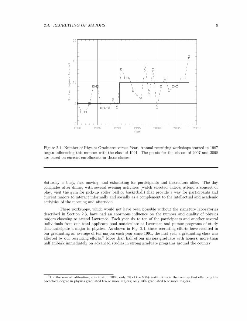
Figure 2.1: Number of Physics Graduates versus Year. Annual recruiting workshops started in 1987began influencing this number with the class of 1991. The points for the classes of 2007 and 2008are based on current enrollments in those classes.
Saturday is busy, fast moving, and exhausting for participants and instructors alike. The dayconcludes after dinner with several evening activities (watch selected videos; attend a concert orplay; visit the gym for pick-up volley ball or basketball) that provide a way for participants andcurrent majors to interact informally and socially as a complement to the intellectual and academicactivities of the morning and afternoon.
These workshops, which would not have been possible without the signature laboratoriesdescribed in Section 2.3, have had an enormous influence on the number and quality of physicsmajors choosing to attend Lawrence. Each year six to ten of the participants and another severalindividuals from our total applicant pool matriculate at Lawrence and pursue programs of studythat anticipate a major in physics. As shown in Fig. 2.1, these recruiting efforts have resulted inour graduating an average of ten majors each year since 1991, the first year a graduating class wasaffected by our recruiting efforts.2 More than half of our majors graduate with honors; more thanhalf embark immediately on advanced studies in strong graduate programs around the country.
2For the sake of calibration, note that, in 2003, only 6% of the 500+ institutions in the country that offer only thebachelor’s degree in physics graduated ten or more majors; only 23% graduated 5 or more majors.

10 CHAPTER 2. THE INSTITUTIONAL AND DEPARTMENTAL CONTEXT

Chapter 3
The Computational Components ofthe Lawrence Curriculum
Computers have been used in physics instruction at Lawrence since 1964 when students in theintroductory courses were sent, card deck in hand, to the institution’s IBM 1620 computer to solveordinary differential equations, find energy eigenvalues for the quantum harmonic oscillator, andanalyze experimental data. Teletype terminals to a time-shared computer came along in 1969 and thefirst institutionally owned time-shared computer—a Digital Equipment Corporation (DEC) PDP 11-45—was installed in the early 1970s. Some of these early uses were spurred by Professor Cook’sfirst sabbatical in 1971–72 at Dartmouth College, then a leader in educational applications of time-shared computing. More consciously structured efforts to bring computing into the entire curriculumtrace to the first Computational Physics Laboratory (CPL) in 19881 and the first equipping of theintroductory laboratory with computers and hardware for on-line data acquisition in 1990.2 Sincethat time, the hardware in the introductory laboratory has been changed twice and and the hardwarein the CPL has been changed three times. These two facilities now provide the infrastructure fornearly all of the current uses of computers in our instructional program.
In broad outline, freshman prospective majors encounter LoggerPro[20], Kaleidagraph, andExcel for data acquisition and analysis, curve fitting, and graphical visualization. Fall-term sopho-mores in Electronics encounter Multisim 7 for circuit simulation and continue to use Kaleidagraphand Excel ; winter-term sophomores in Computational Mechanics experience a concentrated ex-posure to IDL, MAPLE, and LATEX for solving ODEs, evaluating integrals, visualizing functionsgraphically, and preparing neatly printed problem solutions; and spring-term sophomores in Elec-tromagnetic Theory continue to use IDL and MAPLE for graphical visualization and for numericalsolution of Laplace’s equation. Junior/senior courses in quantum mechanics, advanced laboratory,computational physics, mathematical methods of physics, plasma physics, and advanced mechanicsmake further explicit use of computers, though the extent of those uses varies with the instructor. Inaddition, at all points in our curriculum, students are free to use the resources of the CPL wheneverthey deem it appropriate or useful, and many do so in Advanced Laboratory, senior independentprojects, and many other contexts. Indeed, our primary objective in incorporating an early—andsubstantial—explicit introduction to computation is to make sure our students develop sufficientskills early enough in their studies at Lawrence to assure that, ultimately, they will have the neces-sary knowledge and the personal confidence to pursue computational approaches fluently, effectively,and independently on their own initiative.
1The CPL is fully described in Appendix A; financial support is acknowledged on page vii in the preface.2The configuration of hardware and software in this introductory laboratory is described in Section 3.2 and in
footnote 3 in that section; financial support is acknowledged on page vii in the preface.
11

12 CHAPTER 3. THE COMPUTATIONAL COMPONENTS . . .
Term I Term II Term III
Fresh Freshman Studies Freshman Studies ElectiveElective *Intro Classical Physics *Intro Modern Physics
Calculus I Calculus II Calculus III
Soph *Electronics *Computational Mechanics *E and MDiff Eq/Lin Alg Elective Elective
Elective Elective Elective
Junior *Quantum Physics Elective *Advanced LabElective Elective Physics ElectiveElective Elective Elective
Senior Capstone Physics Elective ElectiveElective Elective ElectiveElective Elective Elective
Available Physics Electives:
Group 1: Thermal Physics, Optics, Advanced Mechanics, Advanced E and M, MathematicalMethods of Physics, Advanced Modern Physics, Plasma Physics, Solid State Physics, LaserPhysics, Computational Physics, Tutorials.
Group 2: Independent Studies/Capstone.
Table 3.1: Typical Program of a Physics Major. Courses in bold type are required for a minimummajor in physics; courses marked with an asterisk direct students explicitly to the computer and, inmost cases, include some instruction in one or more of our computational resources.
3.1 Typical Program for Physics Majors
An efficient way to describe the Lawrence approach is to track the computational experience ofmatriculating freshman physics majors as they move towards graduation four years later. Eachyear, full-time students at Lawrence take three courses in each of three ten-week terms. Classperiods are 70 minutes long, and a one-term course is treated officially as the equivalent of a 3-1/3semester-hour course. While there are many variations, the typical program of a student pursuinga physics major is shown in Table 3.1, in which courses marked with an asterisk direct studentsexplicitly to the computer and the ten physics and four mathematics courses shown in bold typeare required for a minimum major in physics, though the occasional matriculant will have sufficientbackground to justify bypassing one or two introductory courses, especially in calculus. Seven toten of the (unqualified) electives will be chosen to satisfy various general education requirements.On the order of ten electives (28% of the student’s program) are completely unconstrained by therequirements for the Lawrence degree or for the major in physics, though most of our (typically)ten graduates each year will take courses in physics, mathematics, and computer science beyondthe minimum required for the major. In addition, many will elect to undertake a senior capstoneproject which, however, is not currently required for the major.

3.2. THE FRESHMAN YEAR (PHYSICS 150, 160) 13
Available physics electives, most of which are offered every other year, are also shown inTable 3.1. Computational Physics makes extensive use of the CPL; in the rest of these courses, stu-dents are free—and are often encouraged—to use those resources on their own initiative (and manyuse them regularly, particularly for graphical visualization and preparation of problem solutions andpapers). Majors are required to take three courses from the eleven in Group 1 and may take asmany as five more from Groups 1 and 2 before exceeding an institutionally imposed limit of fifteencourses in any single department. Tutorials and independent studies, the latter being elected byabout half of all senior majors and sometimes extending over more than one term and leading tohonors in independent study at graduation, offer a vehicle for students to study topics not includedin our regular course offerings.
Beyond our regular curriculum during the academic year, we encourage majors to seekscientifically significant research experiences during the summers. Each summer, four to six studentswho are rising juniors or rising seniors will be engaged as research assistants to Lawrence physicsfaculty members and, occasionally, a rising sophomore will be offered that opportunity. In addition, afew (again four to six) Lawrence physics majors will accept offers to participate in REU programs atother institutions around the country or in industrial or government laboratories. These off-campuspositions are usually limited to rising seniors.
3.2 The Freshman Year (Physics 150, 160)
As freshmen, prospective physics majors at Lawrence first encounter computational approachesin the introductory, calculus-based courses (Physics 150, 160). The infrastructure supporting thecomputational components in these courses (and, incidentally, the computational components inseveral introductory and outreach courses for non-majors) is housed in the introductory physicslaboratory.3 Computer-related hardware in that laboratory now consists of eight Hewlett-PackardPCs running Windows XP, a Hewlett-Packard monochrome laser printer, LabPro[20] interfaces andseveral sensors from Vernier Software and Technology, and units for gathering data on radioactivecounting rates from Spectrum Technologies, Inc. Students in these courses also use the NanoSurfEasyScan scanning tunneling microscopes and atomic force microscopes that are technically partof our emerging surface physics signature laboratory. Available software includes LoggerPro, Excel,Kaleidagraph, the software for driving the Spectrum Technologies and Nanosurf hardware, Multisim 7for circuit simulation in Electronics, and Praat [21] for spectral analysis of sound waves in Physicsof Music.
In particular, students use LoggerPro, Excel, Kaleidagraph, and image-processing softwareassociated with scanning tunneling microscopes. Exercises assigned in the nine or ten three-hourlaboratory sessions in each term routinely involve
3Computers have been used in this introductory laboratory since the late 1960s, when simple data analysis wasdone on a Lawrence-owned batch-mode IBM 1620 computer, then through teletype access to a remote IBM 360computer, and then on in-laboratory terminals to a succession of Lawrence-owned DEC PDP-11 and VAX timeshared computers. In 1990, an NSF grant for a project undertaken by then Assistant Professor John Gastineau, nowemployed at Vernier Software, supported the acquisition of the first microcomputers (MAC SE30s), Vernier ULI cards,and several sensors, and the laboratory took a large step in the direction of providing freshmen with an exposureto on-line data acquisition, statistical data analysis, and graphical visualization of experimental data. Awarded in1997, a grant from the NSF to Professor David M. Cook provided for the replacement of the original computers with(then) state-of-the-art MAC 7300/180 and G3 computers and the acquisition of additional equipment and softwarefor Fourier analysis. While the proposal resulting in this grant focused on up-grading the introductory laboratoryto support the addition of a full laboratory to Professor Cook’s course Physics of Music, it almost goes withoutsaying that other introductory physics courses benefited from this upgrade. Finally, in the summer of 2004, LawrenceUniversity underwrote the updating of the equipment in this laboratory to its current status.

14 CHAPTER 3. THE COMPUTATIONAL COMPONENTS . . .
• automated data acquisition in several experiments (as described in the next two paragraphs),• statistical data analysis in essentially all experiments (Excel and Kaleidagraph),• least squares fitting of linear and parabolic functions to experimental data in several experi-
ments (Excel and Kaleidagraph),• graphical visualization (Kaleidagraph and software special to data-gathering equipment),• creation of images with computer-controlled NanoSurf EasyScan scanning tunneling micro-
scopes and processing of those images, and• radioactive counting experiments using hardware and associated software for data acquisition
from Spectrum Technologies, Inc.
Physics 150, the first course in this two-term rapidly paced sequence, lists one term ofcalculus as a prerequisite—not a corequisite—and deals with classical physics, mostly mechanicsand electromagnetic theory; its current text is Young and Freedman.4 In the lecture portion of thiscourse, students are occasionally assigned exercises that send them to the laboratory computers forgraphing theoretical results or solving ordinary differential equations via Euler and improved Eulermethods using editable Excel templates supplied by the instructor. By far the bulk of the exposureto computers, however, comes in the laboratory meetings, in which students perform experimentstitled
• Using the Laboratory Computers/Elements of Data Analysis, in which students are introducedto the descriptive statistics associated with multiple measurements of single quantities andto Excel as a tool for recording data and doing the requisite arithmetic to determine thesestatistical parameters.
• Position, Velocity, and Acceleration, in which students explore the relationships among thesekinematic quantities, learn how to work with a sonic ranger, and have their first encounter withon-line data acquisition and graphical display using LabPro interfaces and LoggerPro software.
• Free Fall, in which students use a spark-timer to obtain a record of position versus time for thefirst half-second of the motion of an object falling from rest, enter the 25–30 measured posi-tions manually into Excel, use Excel to calculate velocities and accelerations, copy appropriatevalues into Kaleidagraph, and use several different approaches, including least squares fittingto linear and parabolic functions, to extract measured values of the acceleration of gravity withuncertainties.
• Hooke’s Law and Simple Harmonic Motion, in which students explore the relationship betweenforce and extension and the relationship between period and suspended mass for a Hooke’slaw spring, using Excel and Kaleidagraph to do arithmetic and least squares fitting. Then,using the sonic ranger again, a force probe, and LoggerPro, students return to on-line dataacquisition to explore not only position, velocity, acceleration, and force as functions of timebut also velocity as a function of position (phase plane), force as a function of acceleration(F = ma), and force as a function of extension (F = kx).
• Inelastic Collisions, in which the sonic ranger is again used to gather data on the inelasticcollision of a moving cart with a stationary cart, and Excel and Kaleidagraph are used toassess (1) the applicability of conservation of linear momentum, (2) the agreement betweenexperimentally determined and theoretically predicted graphs of final velocity versus initialvelocity, and (3) the agreement between experimentally determined and theoretically predictedgraphs of final kinetic energy versus initial kinetic energy.
4University Physics (11th Edition), Hugh Young and Roger Freedman (Pearson/Addison-Wesley, San Francisco,2004, ISBN 0-8053-9179-7).
3.2. THE FRESHMAN YEAR (PHYSICS 150, 160) 15
• Ballistic Pendulum (Cenco Apparatus), in which students use the rise of the pendulum tomeasure the velocity of the projectile, then predict the position with uncertainty at which theprojectile will hit the floor when fired across the room, place a target, and then subject theirprediction to experimental test. The computer plays a smaller role in this experiment than inmost others, but still is used for statistical analyses of measured values.
• Charge to Mass Ratio of the Electron, in which students measure the currents (and hence themagnetic fields) necessary to deflect an electron beam of known energy in circles of knownradii and then use least squares fitting of those measurements to extract a value for e/m withuncertainty.
• The Driven String: Resonance and Standing Waves, in which mechanical drivers and suitablesignal generators acquired initially for the course Physics of Music are used to study standingwaves in a vibrating string. Students locate a dozen or more normal modes of oscillation anduse least squares fitting to extract information from graphs of frequency versus mode numberand of wavelength versus mode number.
• Interference: Wavelength of Light with a Steel Rule, in which students scatter a laser beam offof the rulings on a machinist’s scale, measure the positions of the maxima in the interferencepattern on the wall, and use Excel and Kaleidagraph to reduce the data (a fairly complicatednumerical process), plot a suitable graph, perform a least squares analysis, and ultimatelyextract a measurement of the wavelength of the light in the laser beam.
Physics 160, the second course in this two-term sequence, deals with relativity, quantummechanics, solid state physics, and particle physics; its current text is Tipler.5 Students are free touse the laboratory computers as they work on the weekly assignments but, again, the bulk of theexposure to computers comes in the laboratory meetings, in which students perform experimentstitled
• Speed of Light, in which students use a pulsed laser and an oscilloscope in a time-of-flightmeasurement of the speed of light. Excel is used for reduction of the measurements.
• Special Relativity Simulation, in which students use Edwin F. Taylor’s SpaceTime[22] to explorelength contraction, time dilation, velocity addition, and the relativity of simultaneity. Thisexperiment is the only experiment in the introductory course in which students use a computersimulation rather than real physical apparatus.
• The Photoelectric Effect, in which the stopping potential of photoelectrons is measured as afunction of the frequency of the incident light. Least squares fitting of the data leads to adetermination of Planck’s constant and the work function of the photoelectric surface.
• The Bohr Model and the Hydrogen Spectrum, in which students use a diffraction grating tomeasure the wavelength of the lines in the Balmer spectrum. Those wavelengths are thencorrelated with the predictions of the Bohr model. Excel is used for reduction of the measure-ments.
• Electron Impact Excitation of Helium (Franck-Hertz Experiment), in which students determinethe excitation energies for helium initially in its ground state by measuring the current at acollecting ring as a function of the energy of the bombarding electrons, associating peaks inthe resulting current with transition energies in the helium atoms. The computer plays only asmall role in this experiment.
5Modern Physics (4th Edition), Paul A. Tipler and Ralph A. Llewellyn (W. H. Freeman and Company, New York,2003, ISBN 0-7167-4345-0).

16 CHAPTER 3. THE COMPUTATIONAL COMPONENTS . . .
• The Scanning Tunneling Microscope (STM), in which students use a computer-controlledNanoSurf EasyScan STM to generate and examine images of the surface of graphite. Inthis experiment, on-line data acquisition and subsequent data analysis are integrated into asingle program that controls the entire process.
• Alpha, Beta, and Gamma Radiation, in which students use a computer-controlled Geigercounter to explore the penetration of various radiations through different distances in airand in other absorbers.
• Radioactive Decay Rate and Half-Life, in which students use a computer-controlled Geigercounter to measure the activity of a short-lived isotope as a function of time.
• Gamma Spectroscopy, in which students use a scintillation counter and computer-controlledpulse height analysis to measure the gamma ray spectrum emitted by available sources and toidentify the material of those sources by its spectrum
Throughout Physics 150 and 160, students are expected to keep complete, accurate, carefulrecords of their work while in the laboratory, and their laboratory records are graded each week notonly on the accuracy and thoroughness of the physics embodied but also on the quality of the recordas a record of what was done, how it was done, and what was thought along the way. Certainly,this laboratory helps students develop their experimental skills and also their skills at keeping usefulrecords of experimental work. By the end of the freshman year, prospective majors have also begunto develop their skills in the use of computational tools, particularly that subset of such skills ofparticular value in the laboratory.
3.3 The Sophomore Year
Beyond the freshman year, majors—of course—continue to use Excel and Kaleidagraph. A seriousintroduction to “real” computation, however, emerges in the sophomore year. In that year (andthereafter), students have 24/7 access to our Computational Physics Laboratory (CPL), whichis equipped—see Appendix A—with hardware and software in all the categories enumerated inSection 1.1 except PowerPoint and LabView . Fall-term sophomores are introduced explicitly tocircuit simulation in Electronics (Section 3.3.1); winter-term sophomores see several applicationsin Computational Mechanics (Section 3.3.2); and spring-term sophomores see additional uses inElectricity and Magnetism (Section 3.3.3).
3.3.1 Electronics (Physics 220)
The course Electronics (Physics 220) meets three times a week, twice for three-hour laboratorysessions and once for a 70-minute lecture/discussion of the current topic. The bulk of the courseentails constructing various circuits and using assorted measuring instruments (oscilloscopes, signaland function generators, frequency counters, digital voltmeters,and digital multimeters) to examinethe properties of the circuits. About 70% of the course is devoted to analog circuits, including LRCresonant circuits and operational amplifiers, and 30% of the course is devoted to digital circuits. Thetexts are Horowitz and Hill6 and Simpson,7 the first as a primary reference and important additionto the students’ personal libraries and the second for most of the reading.
6Paul Horowitz and Winfield Hill, The Art of Electronics (Cambridge University Press, Cambridge, England, 1989,ISBN 0-521-37095-7), Second Edition.
7Robert Simpson, Introductory Electronics for Scientists and Engineers (Prentice-Hall, Englewood Cliffs, NJ, 1987,ISBN 0-205-08377-3), Second Edition. This book is out of print, but several copies are available in the laboratory.

3.3. THE SOPHOMORE YEAR 17
Throughout the term, students continue to hone their skills with Excel and Kaleidagraph.In addition, early in the course, students are introduced to Multisim 7 software installed on thecomputers in the introductory laboratory and, subsequently, use that software to complete a numberof the weekly problem assignments and, whenever they feel it appropriate, to predict or interpretexperimental results. Each student maintains a careful hand-written laboratory notebook, thoughcomputer-produced graphs and spreadsheets will frequently be taped into that notebook. Towardsthe end of the term, each student writes a journal-quality article on one of the experiments. Mostwill use Microsoft Word for the drafting of this article but a few will by this time have learned—andwill use—LATEX. Many will use Multisim 7 to generate theoretical predictions for comparison withtheir experimental results.
3.3.2 Computational Mechanics (Physics 225)
Prior to the academic year 2002–03, we offered a traditional course in intermediate mechanics, us-ing Symon8 or Barger and Olsson9 as the text. In addition, we offered an elective course calledComputational Tools in Physics, which used locally produced documents10 as the text and, in thatperiod, provided the starting point in our nurturing of our students’ abilities to take full advantageof the resources of the Computational Physics Laboratory (CPL). That full-credit course was of-fered in three 1/3-credit segments, one in each of the three terms of our academic year, and wastaken by sophomores as an overload. Its topics were coordinated with the required courses takenby sophomore majors. The first term focused on acquainting students with the rudimentary capa-bilities of our CPL (the UNIX operating system, array processing and graphical visualization usingIDL, publishing scientific manuscripts using LATEX and Tgif, symbolic manipulations using MAPLE,and circuit simulation using SPICE and was coordinated with Electronics. The second term wascoordinated with the intermediate course in classical mechanics, and focused on symbolic and nu-merical approaches to ordinary differential equations (ODEs). The third term was coordinated withan intermediate course in electricity and magnetism11 and focused on symbolic and numerical in-tegration. Especially for those sophomores who did not elect Computational Tools in Physics, weincluded two short computational workshops—one on IDL and the other on MAPLE—in the re-quired sophomore mechanics course. Thus, all sophomores had at least a small, forced exposure tothe CPL, and some—but unfortunately not all—sophomores had a fully comprehensive introductionto the available capabilities.
Beginning in the academic year 2002–03, the course Computational Tools in Physics wasdiscontinued, and the required sophomore course titled Computational Mechanics (Physics 225),which replaced the course in classical mechanics, became the starting point in our nurturing of ourstudents’ abilities to take full advantage of the resources of the CPL. In brief, this course combinesabout 60% of the material covered in a traditional course in intermediate mechanics with about40% of the orientation to computing covered in the discontinued course Computational Tools inPhysics. The gain lies in the incorporation of the computational elements in a course that is requiredof sophomore majors, thus assuring that all majors have an early introduction to computationalapproaches, making possible the assumption of that background in all subsequent courses, andsupporting independent use of our computational resources even if individual faculty members inlater courses do not make explicit assignments involving those resources.
Computational Mechanics does not, of course, cover all of the topics treated in its prede-cessor. In particular, Lagrangian mechanics and rigid body dynamics were moved to our elective
8Keith Symon, Mechanics (Addison Wesley, Reading, MA, 1971, ISBN 0-201-07392-7), Third Edition.9Vernon D. Barger and Martin G. Olsson, Classical Mechanics: A Modern Perspective (McGraw-Hill, New York,
1995, ISBN 0-07-003734-5), Second Edition10See Chapter 5.11See Section 3.3.3.
18 CHAPTER 3. THE COMPUTATIONAL COMPONENTS . . .
junior/senior course Advanced Mechanics. These topics thus remain available to junior and seniormajors but are not any longer encountered by all majors. We believe, however, that this loss is morethan compensated by the acquaintance all of our majors now have with computational approachesand by their and our ability to exploit computational approaches at many points in our intermediateand advanced curriculum.
Computational Mechanics is discussed in fuller detail in Section 4.1.
3.3.3 Electricity and Magnetism (Physics 230)
In Electricity and Magnetism (Physics 230), which uses Griffiths12 as its text, is almost alwaystaken by students immediately after they complete Computational Mechanics, which is the mainprerequisite. Thus, at the end of their sophomore year, majors have an immediate reinforcingof some of the computational topics addressed in Computational Mechanics. Though the detailsand the extent of computer use depend on the individual instructor, students in Electricity andMagnetism use the CPL for graphical visualization of problem solutions worked out by hand; usesymbolic and numerical integration to evaluate electrostatic potentials, electric fields, and magneticfields; solve the Laplace equation using instructor-supplied templates written in IDL’s language; andreview numerical approaches to trajectory problems (which were treated more fully in ComputationalMechanics).
3.4 The Junior and Senior Years
With Computational Mechanics as a uniform background, subsequent theoretical and experimentalcourses alike offer students many opportunities to continue honing their computational skills and,depending on the instructor, some of these courses will direct students explicitly to the CPL for anoccasional exercise. Techniques for graphical visualization are used routinely on the students owninitiative in Optics, Advanced Mechanics, Advanced Electricity and Magnetism, Mathematical Meth-ods of Physics, and Plasma Physics, all of which are alternate-year elective offerings. Most seniorcapstone projects exploit the resources of the CPL, at least for graphical visualization and prepa-ration of reports. Some recent senior projects, notably those in fluid mechanics, musical acoustics,xray diffraction, mapping of astrophysical data, multiphoton quantum transitions, and theoreticalexplorations of the confinement of non-neutral plasmas, have made extensive use of these facilities.Some physics students use the CPL in conjunction with courses in other departments, particularlymathematics. Further, once students have learned to use LATEX in Computational Mechanics, theyroutinely use that tool for preparation of written papers and reports. All of these uses are facilitatedby our policy of granting sophomore, junior and senior majors 24/7 access to the CPL.
Three upper-level courses make more extensive and explicit use of the computer. Usesin Quantum Mechanics, Advanced Laboratory, and Computational Physics are discussed in Sec-tions 3.4.1, 3.4.2, and Sections 3.4.3 and 4.2, respectively.
12David J. Griffiths, Introduction to Electrodynamics (Prentice-Hall, Upper Saddle River, New Jersey, 1999), ThirdEdition.

3.4. THE JUNIOR AND SENIOR YEARS 19
3.4.1 Quantum Mechanics (Physics 310)
Quantum Mechanics (Physics 310), which uses either Griffiths13 or Cook14 as its text, is almostalways taken by students in the fall term of the junior year and, hence, provides the third term ofa comprehensive, intermediate-level exposure to mechanics, electromagnetic theory, and quantummechanics. As with Electricity and Magnetism, the details and the extent of computer use dependon the individual instructor. Students are always free to use the resources of the CPL on their owninitiative and, by this point in their careers at Lawrence, they have acquired sufficient skill andconfidence that many in fact do see ways to use the computer to support their study of quantummechanics. When one of our more computer-oriented faculty members teaches this course, studentsare explicitly directed to the computer for graphical visualizations of quantum wave functions, reflec-tion and transmission coefficients, . . .; for symbolic and numerical solution of quantum eigenvalueproblems (e.g., infinite and finite depth potential wells, simple harmonic oscillator); for symbolicand numerical determination of the time-evolution of Gaussian wave packets; for symbolic and nu-merical evaluation of integrals to find matrix elements and then, for example, explore perturbationexpansions, selection rules, and the Stark effect for higher values of n than are usually addressed byhand; etc.
3.4.2 Advanced Laboratory (Physics 330)
Technically, the laboratory dimensions of our program are outside the purview of responsibilityfor the author of this report. Nonetheless, the exposure that majors have to computation beforeenrolling in Advanced Laboratory supports their confident use of an assortment of computationalresources in that course and also provides the background that facilitates learning about new com-putational techniques that support experimental science to complement the techniques they havealready learned in support of theoretical science.
The course Advanced Laboratory is required for physics majors and is usually taken byjuniors either in the winter or the spring term. Students work individually, and each has exclusiveaccess to the equipment when working on each experiment. Typically, in ten weeks, each studentdoes three or four experiments. For the sake of a serious exposure to research, each student spendsfour or five weeks on the first experiment and is expected to study the pertinent literature, to do anextremely thorough job of the experiment, to contribute something new to the experiment or exploresome new dimension of the physical system, to keep a careful laboratory record, to prepare a journal-quality paper on the experiment, and to give a talk to the rest of the class on that experiment. Whilenew experiments are added and, occasionally, an experiment will be retired, the current optionsinclude the experiments listed in Table 3.2. Most of these experiments involve use of Kaleidagraphand other graphical visualization tools for examining acquired data, use of LATEX or other publishingpackages for preparing written reports, and use of PowerPoint or equivalent presentation softwarefor preparation of talks. The laboratory is equipped with several computers having interface cardsand with numerous measuring instruments that can output digital signals directly to computers,and many experiments therefore involve on-line acquisition of data and compel the student to figureout how to persuade the physical apparatus to communicate with a computer. Linear, polynomial,and non-linear least squares fitting figures in numerous experiments. Occasionally, students usenumerical simulations to support comparison of theoretical predictions with experimental results.
13David J. Griffiths, Introduction to Quantum Mechanics (Prentice-Hall, Upper Saddle River, New Jersey, 2005,ISBN 0-13-111892-7), Second Edition.
14David M. Cook, Non-Relativistic Quantum Mechanics. This set of notes, whose writing was started in 1967 andwhich has seen numerous revisions over the years, has grown to a full—though as yet unpublished—text. A particularfeature distinguishing the current version from other books at the same level is its incorporation of computationalapproaches alongside the more traditional analytic approaches to addressing quantum mechanical problems.

20 CHAPTER 3. THE COMPUTATIONAL COMPONENTS . . .
• Gamma-Gamma Correlation,• High Tc Superconductivity,• Mossbauer Effect,• Muon Decay,• Compton Effect,• Faraday Rotation,• Optical Pumping in Rubidium,• Xray Diffraction,• Quantum Beats,• Holography,• Child’s Law,
• Saturated-Absorption Spectroscopy,• Non-linear Quantum Optics,• Electrical and Optical Properties of Thin Films,• Alpha and Beta Spectroscopy,• Electron Paramagnetic Resonance,• Scanning Tunneling Microscopy,• Atomic Force Microscopy,• Raman Spectroscopy,• Optogalvanic Spectroscopy,• Population Dynamics in a Laser Plasma, and• Laser Fundamentals.
Table 3.2: Experiments Available in Advanced Laboratory.
Those responsible for developing this course are working to incorporate LabView into some of theexperiments, but that inclusion is not yet available to students.
3.4.3 Computational Physics (Physics 540)
The main computational techniques of importance not included in Computational Mechanics applyto generating and visualizing solutions to partial differential equations (PDEs). Some years ago, wetried to incorporate finite-difference and finite-element approaches to PDEs into our junior/seniorelectives Advanced Electricity and Magnetism and Mathematical Methods of Physics. That effortfailed, first—and primarily—because the necessary sacrifice of other topics (electromagnetic radia-tion from accelerated particles, relativistic formulation of electromagnetic theory, Fourier analysisand complex contour integration, . . .) was ultimately deemed unacceptable, and second because—atthe time—only those students who had elected Computational Tools in Physics had the necessarybackground, so only a few juniors and seniors were prepared to profit from inclusion of those topicsin those courses. Once Computational Mechanics had been introduced and taught for two years,however, all junior and senior majors then indeed had the appropriate background. Rather thanresurrecting our earlier incorporation of computational approaches to PDEs into other courses, how-ever, we introduced a new junior/senior course titled Computational Physics (Physics 540). Thiselective course lists Computational Mechanics as a prerequisite, so students who elect Physics 540can move quickly to serious computation; they need not spend a portion of the course learning howto log in and out, work with a text editor and a publishing package, send files to the printer, andwork with basic numerical and symbolic tools—skills that are critical to successful use of a computerbut at the same time are decidedly peripheral to the computational tasks at hand. In short, to use ananalogy from foreign languages, students come to Physics 540 already knowing the vocabulary andthe grammar, and they can begin right away to use these skills in application to the computationaltopics themselves.
Computational Physics is discussed in fuller detail in Section 4.2.

Chapter 4
Central Courses
Two courses in the Lawrence physics curriculum have substantial computational components. Com-putational Mechanics is offered every year, is required in the winter term of the sophomore year, andprovides all majors with an introduction to the resources of the Computational Physics Laboratory(CPL). Computational Physics is an elective junior/senior course that is offered in alternate years,lists Computational Mechanics as a prerequisite, and serves the 20–25% of our majors who seeka more advanced understanding of computational approaches than is provided by the sophomorecourse. Because these two courses are central to the computational dimensions of the Lawrencecurriculum, they are described more fully in this chapter than in the previous brief description inSections 3.3.2 and 3.4.3, respectively.
4.1 Computational Mechanics (Physics 225)
The main objectives of Computational Mechanics (Physics 225) are conveyed by its catalog de-scription, which asserts that it “introduces symbolic and numerical computation through examplesdrawn mainly from classical mechanics but also from classical electromagnetism and quantum me-chanics” and that it “emphasizes computer-based approaches to graphical visualization, the solutionof ordinary differential equations, the evaluation of integrals, and the finding of eigenvalues andeigenvectors”. Prerequisites for the course are Introductory Classical Physics and Differential Equa-tions and Linear Algebra, which itself has three terms of calculus as prerequisites. The text forthe mechanics component, Notes for Computational Mechanics,1 is written by Professor Cook andis comparable in level and sophistication to Symon2 or Barger and Olsson3 but is abbreviated toinclude only those topics covered in the course; the text for the computational components is Com-putation and Problem Solving in Undergraduate Physics (CPSUP), also written by Professor Cook.4
Over the years, the writing of successive drafts of the materials that ultimately found their way intothe version of CPSUP used for this course and ultimately the writing of that book was supportedby grants from the NSF; the actual design of the course and some of the polishing of the text wassupported by the 2001 grant from the W. M. Keck Foundation.5
1While these notes may ultimately be published, as of December, 2006, they are still very much in draft form.2Keith Symon, Mechanics (Addison Wesley, Reading, MA, 1971, ISBN 0-201-07392-7), Third Edition.3Vernon D. Barger and Martin G. Olsson, Classical Mechanics: A Modern Perspective (McGraw-Hill, New York,
1995, ISBN 0-07-003734-5), Second Edition4Both the development of this book and its customizable structure are described more fully in Chapter 5.5See the section titled Acknowledgments on page vii in the preface for more details on these grants.
21
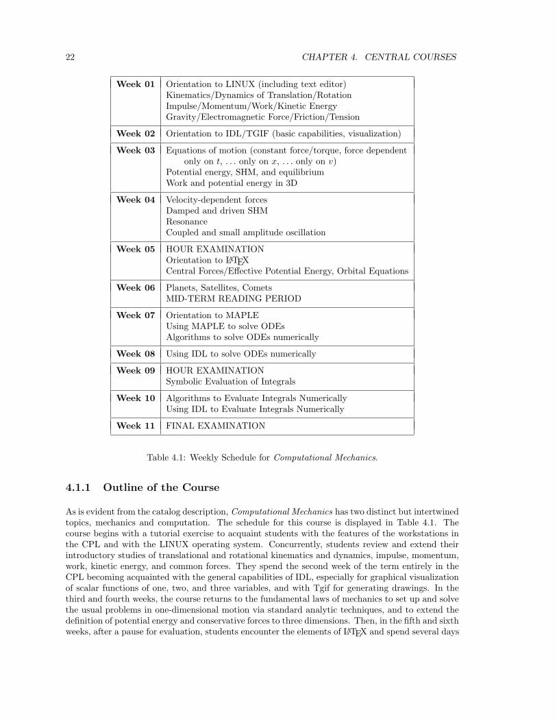
22 CHAPTER 4. CENTRAL COURSES
Week 01 Orientation to LINUX (including text editor)Kinematics/Dynamics of Translation/RotationImpulse/Momentum/Work/Kinetic EnergyGravity/Electromagnetic Force/Friction/Tension
Week 02 Orientation to IDL/TGIF (basic capabilities, visualization)
Week 03 Equations of motion (constant force/torque, force dependentonly on t, . . . only on x, . . . only on v)
Potential energy, SHM, and equilibriumWork and potential energy in 3D
Week 04 Velocity-dependent forcesDamped and driven SHMResonanceCoupled and small amplitude oscillation
Week 05 HOUR EXAMINATIONOrientation to LATEXCentral Forces/Effective Potential Energy, Orbital Equations
Week 06 Planets, Satellites, CometsMID-TERM READING PERIOD
Week 07 Orientation to MAPLEUsing MAPLE to solve ODEsAlgorithms to solve ODEs numerically
Week 08 Using IDL to solve ODEs numerically
Week 09 HOUR EXAMINATIONSymbolic Evaluation of Integrals
Week 10 Algorithms to Evaluate Integrals NumericallyUsing IDL to Evaluate Integrals Numerically
Week 11 FINAL EXAMINATION
Table 4.1: Weekly Schedule for Computational Mechanics.
4.1.1 Outline of the Course
As is evident from the catalog description, Computational Mechanics has two distinct but intertwinedtopics, mechanics and computation. The schedule for this course is displayed in Table 4.1. Thecourse begins with a tutorial exercise to acquaint students with the features of the workstations inthe CPL and with the LINUX operating system. Concurrently, students review and extend theirintroductory studies of translational and rotational kinematics and dynamics, impulse, momentum,work, kinetic energy, and common forces. They spend the second week of the term entirely in theCPL becoming acquainted with the general capabilities of IDL, especially for graphical visualizationof scalar functions of one, two, and three variables, and with Tgif for generating drawings. In thethird and fourth weeks, the course returns to the fundamental laws of mechanics to set up and solvethe usual problems in one-dimensional motion via standard analytic techniques, and to extend thedefinition of potential energy and conservative forces to three dimensions. Then, in the fifth and sixthweeks, after a pause for evaluation, students encounter the elements of LATEX and spend several days

4.2. COMPUTATIONAL PHYSICS (PHYSICS 540) 23
on the standard analytic approaches to the central force problem. The remainder of our ten-weekterm is spent mostly in computationally related activities, including an orientation to MAPLE, adiscussion of numerical algorithms for solving ordinary differential equations (ODEs) and evaluatingintegrals, and an introduction to routines built into IDL for solving ODEs and evaluating integrals.Examples include many of the problems already discussed analytically but also introduce non-linearand chaotic systems. Sample integrals are found in the evaluation of potential energies, momentsand products of inertia, and electric and magnetic fields and potentials. In the rearrangement thatgenerated Computational Mechanics from its predecessor, a more traditional intermediate course inclassical mechanics, only Lagrangian mechanics and rigid-body dynamics were omitted to providethe time for the addition of the computational topics. In the Lawrence curriculum, these two topicsare included in an elective alternate-year, junior/senior elective titled Advanced Mechanics.
Computational Mechanics is a rapidly paced and intensive course. Students in the coursespend quite a bit of time in the CPL. Especially during the first few weeks of the term, whenstudents are inexperienced with the available computational tools, we arrange for a more experiencedstudent—often a student who had worked as a research assistant to Professor Cook in the previoussummer—to be available in the CPL for four to six scheduled hours each week to help studentsin the course strengthen their wings so that, later in the term, they can be expected to fly moreconfidently on their own.
4.1.2 Sample Problems from Assignments
Because they refer to chapters and exercises from the texts, detailed syllabi for this course would notbe particularly meaningful and are not included in this report. Instead, to give a bit of the flavor ofthe course, several representative problems assigned during the term are collected in Appendix B.Note that, after students have learned a bit of LATEX in week 5, they are required to complete theirsolutions to one or two problems each week using that publishing tool.
4.1.3 Examinations from a Recent Offering
The examinations given in a recent offering of this course also convey something of the expectations.In each offering, there are two one-hour examinations and one three-hour final examination. Thesecond of the two hour examinations typically contains both an in-class, closed-book timed part andan out-of-class, open-book but closed-classmate, at-the-computer part. The first hour examinationmay or may not have an at-the-computer component and, because the enrollment in the courseexceeds the available equipment, the final examination will not involve any work at the computer.The first hour examination and the final examination, however, may well ask students to lay outwhat they would do were they able to access a computer. Copies of the three examinations fromthe winter, 2006, offering of Computational Mechanics are contained in Appendix C.
4.2 Computational Physics (Physics 540)
The main objectives of this alternate-year offering are conveyed by its catalog description, whichasserts that it “treats computational approaches to problems in physics with particular emphasis onfinite-difference and finite-element methods for solving partial differential equations as they arise inelectromagnetic theory, fluid mechanics, heat transfer, and quantum mechanics, and on techniquesfor graphical visualization of the solutions”. The prerequisite for the course is Computational Me-chanics, which simple statement hides the several physics and mathematics prerequisites for the

24 CHAPTER 4. CENTRAL COURSES
stated prerequisite course. The text for the course is Professor Cook’s CPSUP, supplemented withassorted documentation for the various programs used during the course. The development of thiscourse and the drafting and revising of the portions of CPSUP used in this course were supportedby the 2001 grant from W. M. Keck Foundation.6
4.2.1 Outline of the Course
The daily schedule for Computational Physics is compiled in Table 4.2. Because students spend quitea lot of time at the workstations in the CPL and because it usually doesn’t take very long in classto set the stage for lengthy exercises at the computer, this course meets for lecture on average 1.5times per week. At other times, students work on the regular assignments, which are common to allstudents and involve (relatively) straightforward exercises that invoke the computational strategy ofthe week. The course begins by orienting students, all of whom have taken Computational Mechanicsbut most of whom have not taken a formal course in programming, to the elements of structuredprogramming, first in pseudocode (which allows focusing on concepts rather than syntactic details)and then in FORTRAN and IDL.
After spending a day and a half deriving the standard second-order partial differential equa-tions of mathematical physics (wave equation, diffusion equation, Laplace equation) and discussingthe multitude of physical contexts in which one or another of these equations appears, the courseintroduces finite difference methods and applies them to
• discretize the diffusion equation in the spatial coordinate(s) but not the temporal coordinate,yielding a possibly large set of first-order ordinary differential equations to be solved simulta-neously subject to appropriate initial and boundary conditions. (The solution of ODEs usingIDL was treated in Computational Mechanics; in Computational Physics, students review useof IDL but then move to using the large FORTRAN solver LSODE, which gives them theirfirst experience writing driving programs to invoke existing and well tested subroutines.)
• discretize the wave equation in the spatial coordinate(s) but not the temporal coordinate,yielding a possibly large set of second-order ordinary differential equations to be solved simul-taneously subject to appropriate initial and boundary conditions.
• discretize the Laplace equation in all coordinates, yielding a possibly large set of algebraicequations to be solved by an iterative approach. Students first follow a supplied template towrite programs, either in IDL or FORTRAN or C, to implement the standard iteration fora variety of different boundary conditions and geometries. Later in the term, students learnabout multigrid approaches to speed the convergence of the iteration and, instead of trying tocode this more difficult approach themselves, encounter again the need to write driving pro-grams to invoke existing subroutines, this time MUD2SP and MUD3SP from the MUDPACKpackage of solvers for elliptic partial differential equations in two and three dimensions.
• discretize the wave and diffusion equations in all coordinates, obtaining a set of algebraicequations that support the systematic stepping of the initial values indefinitely into the futureand, following templates developed in lectures and the text, write their own IDL or FORTRANor C code to solve a number of problems with different initial and boundary conditions.
About 35% of the time in our ten-week term is devoted to this segment of the course.
The final topic of the course, to which about 30% of the time is devoted, addresses finiteelement approaches to partial differential equations though, for simplicity of the initial development,
6See the section titled Acknowledgements on page vii in the preface for more details on these grants.

4.2. COMPUTATIONAL PHYSICS (PHYSICS 540) 25
Day 01 Programming Structures and Strategies
Day 02 Programming in FORTRAN and IDLDay 03 Analytic/Physical Derivation of PDEs (wave,
diffusion, Laplace, and fluid dynamics equations)Day 04 Finite Difference Methods (Part I)
Day 05 ASSIGN 1 DUE; Driving Programs for LSODE (Part I)Day 06 Driving Programs for LSODE (Part II)Day 07 No class; Work on Assignment 2
Day 08 ASSIGN 2 DUE; Finite Difference Methods (Part II)Day 09 Finite Difference Methods (Part III)Day 10 No Class; Work on Assignment 3
Day 11 No Class; Work on Assignment 3Day 12 Oral presentations on Assignment 3Day 13 ASSIGN 3 DUE; MUDPACK/Multigrid Techniques (Part I)
Day 14 MUDPACK/Multigrid Techniques (Part II)Day 15 No Class; Work on Assignment 4Day 16 ASSIGN 4 DUE; Finite Element Methods (Part I)
Day 17 Finite Element Methods (Part II)Day 18 Finite Element Methods (Part III)Day 19 MID-TERM READING PERIOD; No Class
Day 20 No Class; Work on Assignment 5Day 21 ASSIGN 5 DUE; FEMs with MARC/MENTAT (Part I)Day 22 FEMs with MARC/MENTAT (Part II)
Day 23 Project Proposal Due; No Class; Work on Assignment 6Day 24 Oral Presentations on Assignment 6Day 25 ASSIGN 6 DUE; No Class; Work on Projects
Day 26 No Class; Work on ProjectsDay 27 THANKSGIVING VACATIONDay 28 THANKSGIVING VACATION
Day 29 No Class; Work on ProjectsDay 30 No Class; Work on ProjectsDay 31 Oral Presentations on Projects; Final Paper Due
No Final Examination
Table 4.2: Daily Schedule for Computational Physics. The vertical blocking corresponds to theweeks of the term, which happened to start on a Friday in the year to which this schedule applies.
the approach is first applied to ordinary differential equations. In both one and two dimensions, thedevelopment of the technique focuses on a general second-order, self-adjoint, linear, inhomogeneousequation. The overall strategy is laid out, and templates for coding in FORTRAN and IDL areworked out for specific examples of such equations, and students then modify those templates toadapt them to other examples. After the technique has been described and practice with very simpleexamples completed, the course spends two days describing how to use a pair of commercial programs

26 CHAPTER 4. CENTRAL COURSES
called MARC (a venerable solver of partial differential equations by finite element methods) andMENTAT[23] (a more contemporary GUI interface for defining problems, automeshing the geometry,creating the input file for MARC, and examining the output produced by MARC). Students thencomplete an assignment that asks them to adapt strategies illustrated in the class discussion ofMARC/MENTAT to slightly different situations.
4.2.2 The Projects
Because they refer to chapters and exercises from the texts, detailed syllabi would not be particularlymeaningful and are not included in this report. Further, no examinations are given in this course.Beyond the weekly written assignments (which all students complete using LATEX), students alsocomplete two medium-length projects, the first (a component of Assignment 3) an assigned projectusing finite difference techniques and the second (a component of Assignment 6) an assigned projectusing finite element techniques. At the end of the term (the entirety of Assignment 7), each studentcompletes a final, longer project of his or her choice but subject to the instructor’s advance approval.On each of these projects, each student prepares an oral presentation (15 minutes for the first twoprojects; 25–30 minutes for the end-of-term project) delivered to the class and also a written paper.The general level of the course and the types of problem that students are expected to be ableto address are conveyed by the portions of the assignments describing these three projects. Thoseportions of Assignments 3, 6, and 7 are presented in Appendix D.

Chapter 5
CPSUP
The computational components of the Lawrence curriculum and the text which is the topic of thischapter evolved together, and the text has played an important role in supporting our curriculardevelopments. Titled Computation and Problem Solving in Undergraduate Physics (CPSUP),1 thetext had its origins in the mid 1980s when, as has been detailed in the previous chapters of thisreport, we at Lawrence decided that, to be properly prepared for their future careers in physics, ourmajors needed to have a substantial exposure to computational approaches to problems alongsidethe more traditional analytic approaches and they needed to have that exposure early enough sothat we could require them to use computational resources in subsequent courses and so that theywould have the knowledge and confidence to use those resources on their own initiative wheneverit seemed to them appropriate to do so. In the first decade of this project, activities focused onacquiring hardware and software, developing a succession of curricular modifications, and generatingnumerous—ultimately 65 or 70—documents that described the features of the operating system andthe several acquired software packages and illustrated how to apply those software packages—bothsymbolic and numeric—to selected representative problems drawn from several different subareas ofphysics.
By late 1998, it was clear that developments at Lawrence might well be of interest to thewider community—a realization that prompted the submission of a proposal to the EducationalMaterials Development (EMD) track of the CCLI program of the NSF.2 The objectives of theproposed activity were
• to standardize the format of and expand the extensive library of instructional materials devel-oped at Lawrence into a flexible publication to support introduction of uses of computationalresources into the upper-level undergraduate physics curriculum;
• to conduct week-long summer workshops for physics faculty from around the country, not onlyfor evaluation and assessment but also for dissemination; and
• to publish the final product.
The bulk of the writing took place during the summers of 2000, 2001, and 2002 and during a sabbat-ical year early in that period. In the summers, student assistants drafted solutions to representativeexercises. Thus, the end result is not only a book, which runs to about 900 pages if all components
1Greater detail about CPSUP can be found at the URL http://www.lawrence.edu/dept/physics/ccli. A reviewwas published in the American Journal of Physics, Vol. 74, No. 7 (July, 2006), pp. 653–655.
2See NSF Grant DUE-9952285 as listed in the section titled Acknowledgements on page vii in the preface.
27

28 CHAPTER 5. CPSUP
are included, but also an accompanying manual containing solutions to nearly 200 representativeexercises.
In this chapter, the text itself is described in fuller detail. While the writing of this text wasprompted by the absence of curricular materials appropriate to what we wanted to do at Lawrence,the attempt in the final version was to create a text that would have potential use in a varietyof contexts. In this chapter, we state the challenges, describe the structure of the resulting book,speculate about possible uses of CPSUP, describe the strategy adopted for meeting the publishingchallenge, and outline the future growth of CPSUP.
5.1 The Challenges
That different departments use different hardware and software poses a major challenge to thewriting of a widely useful text. The variety of options and combinations is so great that any singlechoice (or coordinated set of choices) is bound to limit the usefulness of the end result to a smallsubset of all potentially interested users. The strategy adopted by CPSUP to address this challengeinvolves assembling different versions of the basic materials from a wide assortment of components,some of which—the generic components—will be included in all versions and others of which—thosespecific to particular software packages—will be included only if the potential user requests them.Thus, the specific software and hardware treated in any particular version will be microscopically“tailor-able” to the spectrum of resources available at the user’s site. One version, for example,could include the generic components and only the components that introduce the features of andapply IDL, MAPLE, C, and LATEX while another might include the generic components and thecomponents that introduce the features of and apply MATLAB, MATHEMATICA, and FORTRAN(including Numerical Recipes).
A second challenge arises because, even among sites that use the same hardware andsoftware, some aspects of local environments are still unique to individual sites. Rules of citizenship,practices and policies regarding accounts and passwords, the features and elementary resources ofthe operating system, the structuring of public directories, backup schedules, after-hours access,licensing restrictions in force on proprietary software, and numerous other aspects are subject toconsiderable local variation. CPSUP itself makes no attempt to address this challenge and doesnot constrain local options in these matters. Throughout the book, individual users are directedto a publication called the Local Guide for site-specific particulars. A suggested template for thatguide will be provided. This guide will have to be created at each site, though a template for thatguide—specifically, the guide used at Lawrence—accompanies CPSUP.
Third and fourth challenges are consequences of the microscopic customizability. Themarket for any single version is likely to be small. Thus, any potential publisher must be ablenot only to assemble and print the desired version on demand (the third challenge) but also (thefourth challenge) to respond economically to orders for relatively small numbers (5–10) of copies ofa particular version. The author’s way to address these challenges is laid out in Section 5.5.
5.2 The Structure of CPSUP
The essential idea for the book emerged from a recognition that the background for and setup ofparticular problems to be addressed with a computer are independent of the specific hardware onwhich and software package with which the solutions would be pursued. It ought therefore to bepossible to create a single book that could be produced in various versions. The book would beassembled from generic components that would be common to all versions and software-specific

5.2. THE STRUCTURE OF CPSUP 29
Chapter 1. PreliminariesChapter 2. Introduction to IDLChapter 3. Introduction to MATLABChapter 4. Introduction to MACSYMAChapter 5. Introduction to MAPLEChapter 6. Introduction to MathematicaChapter 7. Introduction to ProgrammingChapter 8. Introduction to Numerical RecipesChapter 9. Solving Ordinary Differential EquationsChapter 10. Introduction to LSODEChapter 11. Evaluating IntegralsChapter 12. Finding Roots
Appendix A. Introduction to LATEXAppendix B. Introduction to TGIF
Table 5.1: Top-Level Table of Contents for CPSUP.
components, different subsets of which would appear in different versions. At the coarsest level,that flexibility is illustrated in the top-level table of contents in Table 5.1. Chapter 1 stands alone;Chapters 2 and 3 introduce the general features of two common array processors; Chapters 4, 5, and6 introduce the features of three different computer algebra systems; Chapters 7 and 8 introduce aprogramming language and the numerical recipes library; Chapters 9, 10, 11, and 12 address severalimportant categories of computational processing; and the appendices introduce a publishing systemand a program for producing drawings. Any particular version would include at least one of Chapters2 and 3 and one of Chapters 4, 5, and 6, and Chapters 9, 11, and 12—though these last three wouldbe assembled with only those components that illustrate the programs included in the selectionsfrom Chapters 2–6. Chapters 7, 8, and 10, the associated sections in Chapters 9, 11, and 12, andthe appendices would be included only if desired by the end user. While the pedagogic objective isfor students to become fluent in the use of a spectrum of computational tools, and the chapters areorganized by program or by computational technique, the focus throughout is on physical contexts.
The top-level table of contents, however, does not accurately convey the full structure ofthe text. Chapters fall into two groups. Each of Chapters 2, 3, 4, 5, 6, 8, and 10 and AppendicesA and B, for example, focuses on the basic features of a particular application program. Thoughthese chapters draw their examples from physical situations and conclude with numerous physicallyoriented exercises, they still focus on the capabilities of the application program rather than onthe physics illustrated in the examples. Their format reflects a conviction that students must firstfocus attention on the application program itself before being ready to use the program to addressproblems in physics. For example, Chapter 3, the table of contents of which is shown in Table 5.2,is representative of chapters in this group. Specifically, Chapter 3 introduces the main features ofMATLAB, a program for processing arrays of numbers and creating graphical visualizations of one-,two-, and three-dimensional data sets. The other chapters in this group have a similar structure.Many of the sections in these chapters are structured as tutorials that lead the reader through themain features of the corresponding program, are to be studied at a computer, and lean in somemeasure on vendor-supplied documentation and on-line help to encourage and guide self-study.
Shown in Table 5.3, the structure of Chapter 11 on evaluating integrals exemplifies thestructure of the chapters in the second group, each of whose members focuses on a particularcomputational technique. Presumably, before approaching any particular section in this chapter,the student would have studied the relevant sections in earlier chapters. The first section in each ofthese chapters (here Section 11.1) sets several physical problems, the successful addressing of which
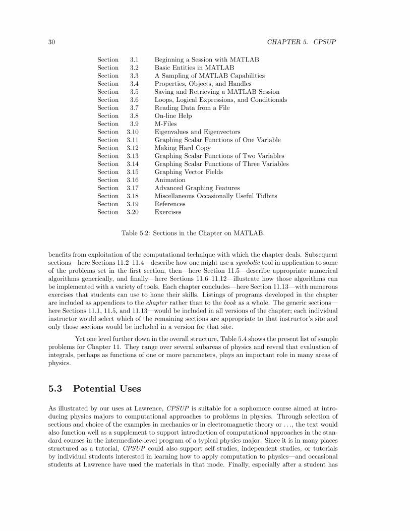
30 CHAPTER 5. CPSUP
Section 3.1 Beginning a Session with MATLABSection 3.2 Basic Entities in MATLABSection 3.3 A Sampling of MATLAB CapabilitiesSection 3.4 Properties, Objects, and HandlesSection 3.5 Saving and Retrieving a MATLAB SessionSection 3.6 Loops, Logical Expressions, and ConditionalsSection 3.7 Reading Data from a FileSection 3.8 On-line HelpSection 3.9 M-FilesSection 3.10 Eigenvalues and EigenvectorsSection 3.11 Graphing Scalar Functions of One VariableSection 3.12 Making Hard CopySection 3.13 Graphing Scalar Functions of Two VariablesSection 3.14 Graphing Scalar Functions of Three VariablesSection 3.15 Graphing Vector FieldsSection 3.16 AnimationSection 3.17 Advanced Graphing FeaturesSection 3.18 Miscellaneous Occasionally Useful TidbitsSection 3.19 ReferencesSection 3.20 Exercises
Table 5.2: Sections in the Chapter on MATLAB.
benefits from exploitation of the computational technique with which the chapter deals. Subsequentsections—here Sections 11.2–11.4—describe how one might use a symbolic tool in application to someof the problems set in the first section, then—here Section 11.5—describe appropriate numericalalgorithms generically, and finally—here Sections 11.6–11.12—illustrate how those algorithms canbe implemented with a variety of tools. Each chapter concludes—here Section 11.13—with numerousexercises that students can use to hone their skills. Listings of programs developed in the chapterare included as appendices to the chapter rather than to the book as a whole. The generic sections—here Sections 11.1, 11.5, and 11.13—would be included in all versions of the chapter; each individualinstructor would select which of the remaining sections are appropriate to that instructor’s site andonly those sections would be included in a version for that site.
Yet one level further down in the overall structure, Table 5.4 shows the present list of sampleproblems for Chapter 11. They range over several subareas of physics and reveal that evaluation ofintegrals, perhaps as functions of one or more parameters, plays an important role in many areas ofphysics.
5.3 Potential Uses
As illustrated by our uses at Lawrence, CPSUP is suitable for a sophomore course aimed at intro-ducing physics majors to computational approaches to problems in physics. Through selection ofsections and choice of the examples in mechanics or in electromagnetic theory or . . ., the text wouldalso function well as a supplement to support introduction of computational approaches in the stan-dard courses in the intermediate-level program of a typical physics major. Since it is in many placesstructured as a tutorial, CPSUP could also support self-studies, independent studies, or tutorialsby individual students interested in learning how to apply computation to physics—and occasionalstudents at Lawrence have used the materials in that mode. Finally, especially after a student has

5.3. POTENTIAL USES 31
Section 11.1 Sample ProblemsSection 11.2 Evaluating Integrals Symbolically with MACSYMASection 11.3 Evaluating Integrals Symbolically with MAPLESection 11.4 Evaluating Integrals Symbolically with MathematicaSection 11.5 Algorithms for Numerical IntegrationSection 11.6 Evaluating Integrals Numerically with IDLSection 11.7 Evaluating Integrals Numerically with MATLABSection 11.8 Evaluating Integrals Numerically with MACSYMASection 11.9 Evaluating Integrals Numerically with MAPLESection 11.10 Evaluating Integrals Numerically with MathematicaSection 11.11 Evaluating Integrals Numerically with FORTRANSection 11.12 Evaluating Integrals Numerically with CSection 11.13 Exercises
Appendix 11.A Listing of trapezoidal.fAppendix 11.B Listing of trapezoidal.c
Table 5.3: Sections in the Chapter on Integration.
11.1.1. One-Dimensional Trajectories11.1.2. Center of Mass11.1.3. Moment of Inertia11.1.4. Large-Amplitude Pendulum (Elliptic Integrals)11.1.5. The Error Function11.1.6. The Cornu Spiral11.1.7. Electric/Magnetic Fields and Potentials11.1.8. Quantum Probabilities
Table 5.4: Sample Problems in Section 11.1.
spent some time with some of the chapters, CPSUP should be a useful reference work to have inone’s library. Broadly, CPSUP is a flexible text that can be used in a variety of ways—including asthe text for stand-alone courses, as a supplement to existing courses, and as the text for tutorials andself-study—to support introduction of computational approaches to problems in physics alongsidethe more traditional analytic approaches.
While the motivation throughout CPSUP lies in and all examples are drawn from physicalcontexts, the ultimate objective is for students to develop a sound understanding of the capabilitiesof a spectrum of computational tools, of a variety of computational techniques, strategies, andalgorithms, and of the ways in which those capabilities and techniques can be productively exploitedto address serious and substantial problems in physics. Students cannot profitably attempt to runin this arena, however, before they have learned to walk. While CPSUP draws its examples fromphysical contexts and students working their way through the book will learn physics, the bookassumes that the student has completed at least an introductory calculus-based survey course inphysics to justify placing the greater emphasis on the computational tools and techniques. Thatfocus also leads to a two-fold organization based on the most important capabilities of the tools andon generally useful computational techniques rather than on the standard subdisciplines of physics.The typical user will jump around in CPSUP to study only those sections that relate to availablesoftware packages, only those illustrative exercises that apply to the particular subdiscipline ofphysics of concern. Though some of the later sections in the book depend on some earlier sections,the linkages are not particularly tight. Thus, the order of presentation in the book does not compel

32 CHAPTER 5. CPSUP
any particular order of treatment in a course or program of self-study.
5.4 Workshops
For purposes of both evaluation and dissemination, the 2000 NSF grant and its 2003 supplementsupported four week-long summer workshops at Lawrence. In each workshop, participants racedthrough exercises that familiarized them with the Lawrence computational environment, with theprimary features of IDL or MATLAB (1 day), and of MAPLE or MATHEMATICA (1 day), andthen with applications of these programs to address problems in physics involving ordinary differen-tial equations (1 day), evaluation of integrals as functions of parameters (1 day), and finding roots(1 day). A total of seventy faculty members representing sixty-six distinct physics departmentsfrom around the country participated in these workshops and provided feedback on the growingmanuscript. A few served more formally as beta testers, and several are among those who havecontinued to use CPSUP in the years after its completion. Dissemination also occurred as a con-sequence of talks and posters—see a full listing in Appendix A.6—presented at national meetingsand occasional announcements emailed and/or US-mailed to the chairs of departments offering thebachelor’s degree in physics and others on a growing locally maintained mailing list.
5.5 Addressing the Publishing Challenge
Present-day customizable and print-on-demand publishing is not yet capable of providing the mi-croscopic section by section customization that CPSUP requires, especially when the number ofcopies ordered of any particular version is likely to be small (5–20). Until an on-going search for acommercial publisher meets with success, the book is being self-published by the author.3 With theassistance of TEX, LATEX, and an assortment of associated pieces of software, the process of producinga PostScript file containing the generic components and the selected software-specific components forany particular version is almost trivially easy. Once all the appropriate LATEX source files containingthe text of the various components (with embedded formatting and indexing commands) have beencreated and, in addition, a buyer-specific file containing true/false values for the flags that select thecomponents to be included is available, the process involves
• running LATEX,• running LATEX a second time to set the internal cross references and table of contents correctly,• running LATEX a third time, especially if insertion of the proper internal references in the
second pass causes the pagination to change,4
• running makeindex to generate the file from which the index will be produced,• running LATEX one last time (third or fourth time) to produce an output file that contains the
proper index, and• running dvips.
After about five minutes of processor time on a contemporary desktop computer, the PostScript filefor a 400–900 page book is in hand!!! That file is then sent electronically to a nearby commercialprint shop, whose staff members provide it as input to a fascinating machine that digests the file andproduces bound copies as output, all without human intervention. That commercial establishment
3Self-publishing has its drawbacks, but one advantage of the approach and the associated on-demand printing isthat typos, grammatical infelicities, and unclear passages discovered now and then can be corrected immediately andbe right in all subsequent printings.
4The system prints a warning during the second pass if a third pass is necessary.
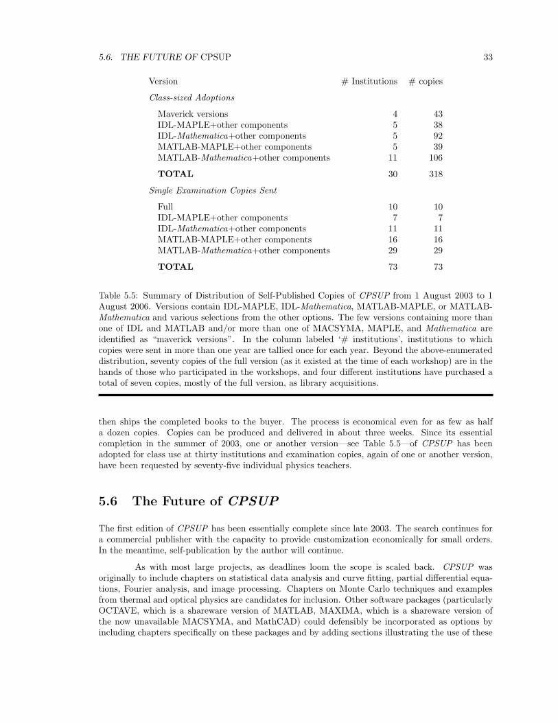
5.6. THE FUTURE OF CPSUP 33
Version # Institutions # copies
Class-sized Adoptions
Maverick versions 4 43IDL-MAPLE+other components 5 38IDL-Mathematica+other components 5 92MATLAB-MAPLE+other components 5 39MATLAB-Mathematica+other components 11 106
TOTAL 30 318
Single Examination Copies Sent
Full 10 10IDL-MAPLE+other components 7 7IDL-Mathematica+other components 11 11MATLAB-MAPLE+other components 16 16MATLAB-Mathematica+other components 29 29
TOTAL 73 73
Table 5.5: Summary of Distribution of Self-Published Copies of CPSUP from 1 August 2003 to 1August 2006. Versions contain IDL-MAPLE, IDL-Mathematica, MATLAB-MAPLE, or MATLAB-Mathematica and various selections from the other options. The few versions containing more thanone of IDL and MATLAB and/or more than one of MACSYMA, MAPLE, and Mathematica areidentified as “maverick versions”. In the column labeled ‘# institutions’, institutions to whichcopies were sent in more than one year are tallied once for each year. Beyond the above-enumerateddistribution, seventy copies of the full version (as it existed at the time of each workshop) are in thehands of those who participated in the workshops, and four different institutions have purchased atotal of seven copies, mostly of the full version, as library acquisitions.
then ships the completed books to the buyer. The process is economical even for as few as halfa dozen copies. Copies can be produced and delivered in about three weeks. Since its essentialcompletion in the summer of 2003, one or another version—see Table 5.5—of CPSUP has beenadopted for class use at thirty institutions and examination copies, again of one or another version,have been requested by seventy-five individual physics teachers.
5.6 The Future of CPSUP
The first edition of CPSUP has been essentially complete since late 2003. The search continues fora commercial publisher with the capacity to provide customization economically for small orders.In the meantime, self-publication by the author will continue.
As with most large projects, as deadlines loom the scope is scaled back. CPSUP wasoriginally to include chapters on statistical data analysis and curve fitting, partial differential equa-tions, Fourier analysis, and image processing. Chapters on Monte Carlo techniques and examplesfrom thermal and optical physics are candidates for inclusion. Other software packages (particularlyOCTAVE, which is a shareware version of MATLAB, MAXIMA, which is a shareware version ofthe now unavailable MACSYMA, and MathCAD) could defensibly be incorporated as options byincluding chapters specifically on these packages and by adding sections illustrating the use of these

34 CHAPTER 5. CPSUP
packages in other chapters. And other languages like Java, publishing packages beyond LATEX, anddrawing programs beyond Tgif should perhaps be made available as options.
Beyond the flexibility easily to accommodate a variety of choices of hardware and soft-ware, the structure adopted has also the convenient—perhaps even fortuitous—capability of easyexpansion. With support from the 2001 W. M. Keck Foundation grant, a step in the direction of asecond edition has already been taken with the drafting of at least parts of the chapters that supportthe course Computational Physics. Chapter 13 on finite difference and finite element approaches topartial differential equations, Chapter 14 on the package MUDPACK, which contains FORTRANsolvers that use multigrid techniques to address elliptic partial differential equations in two andthree dimensions, and Chapter 15 on MARC/MENTAT, which is a commercial pair of programs forsetting up and solving partial differential equations by finite element techniques are well along. Asof December, 2006, the generic parts of these chapters are complete, but the software-specific partsexist only for the software packages in use at Lawrence.
As the author moves towards retirement from full-time teaching, he expects to devotemore of his efforts to filling in these gaps. Chapters on many other computational topics and onother software packages may well come into being. Further, once the publishing wrinkles have beensatisfactorily worked out and the structure of the files has been refined and documented, otherauthors may be attracted to contributing components on their favorite topics or software packages,so the book may expand to offer as options a wider and wider spectrum of hardware and softwareand to include topics not originally incorporated and, more particularly, topics that go beyond theknowledge, skill, and/or energy of the initial author. Periodically, reports of progress on these frontswill be posted on the project website at the URL http://www.lawrence.edu/dept/physics/ccli.

Appendix A
Computational Physics Laboratory
A.1 A Brief History
In 1987, convinced that the scientific careers of its majors would be significantly enhanced by abroad exposure to computational approaches to problems in physics, the Department of Physics atLawrence successfully sought support amounting to about $400,000 from the W. M. Keck Foun-dation, the National Science Foundation, and several vendors to conduct a pilot project designedto nurture both the personal initiative and the individual skills to use sophisticated computationaltools intelligently and independently. To this end, we have created the Lawrence ComputationalPhysics Laboratory (CPL), which gives 45 or so physics majors each year (typically 12 seniors, 13juniors, 20 sophomores) and five faculty members exclusive 24-hour per day access to an impres-sive collection of computational hardware and software as well as a library of pertinent manuals,text books, and locally prepared documents. In addition, we have engaged in faculty development,and—most importantly—we have embedded numerous computer-based classroom demonstrationsand homework exercises in many of our upper-level offerings, thereby encouraging and supportingcontinued independent use both in our junior/senior courses and in senior-level independent studies.This pilot project has received national attention, being described in several published papers andinvited talks (see later section). Its existence served as the basis for convening a small nationalconference (Summer, 1990) at Lawrence (supported by the Sloan Foundation), and it has stimulatedseveral individual visits to the Lawrence campus.
In 1993, additional funds amounting to about $150,000 were received from the NationalScience Foundation and the W. M. Keck Foundation to permit addition of 3D graphics capabilitiesand color printing capabilities to the Computational Physics Laboratory initially equipped by thegrants received in 1987 and 1988.
In 1998, grants from Lawrence University allowed us to begin replacing the oldest SGIequipment with up-to-date SGI equipment. This process will be ongoing, two or three older unitsbeing replaced each year with state-of-the-art equipment.
In early 2000, a grant of $177,026 (supplemented in 2003 with an additional $3781) from theEducational Materials and Development (EMD) track of the Course, Curriculum and LaboratoryImprovement (CCLI) Program of the National Science Foundation provided support for the collectionof numerous local instructional documents into a text and the conduct at Lawrence of four week-long
35

36 APPENDIX A. COMPUTATIONAL PHYSICS LABORATORY
summer workshops for physics faculty members from around the United States. The resulting book,titled Computation and Problem Solving in Undergraduate Physics (CPSUP), is flexible in design.Through the inclusion of components using the selected software packages, the book can be adaptedto respect the particular hardware and software available at specific institutions. Details can befound at the project website at the URL http://www.lawrence.edu/dept/physics/ccli.
In December, 2001, the Department received a third grant from the W. M. Keck Founda-tion. Of the $400,000 total grant, $106,853 was allocated to further development of the CPL. Theprimary objectives of this infusion were to introduce a required sophomore course in computationand mechanics, to introduce an elective junior/senior course in computational physics, and to in-crease the extent to which computational resources are used throughout the physics curriculum atLawrence. In anticipation of increased use generated by those changes in our curriculum, the grantsupported an expansion of the total number of workstations in the laboratory and an upgrading ofthe server, the existing workstations, and the printers.
In the remainder of this appendix, we enumerate the current spectrum of hardware andthe most frequently used pieces of software and list the several papers and presentations that havearisen in the context of developing this resource and writing the text already mentioned.
A.2 Hardware
The first computational physics laboratory, which was constructed in 1988, was equipped with DigitalEquipment Corporation (DEC) VAXstations and a VAXserver running VMS. By the early 1990s,VMS was fading and UNIX was ascending as the operating system of choice for scientific workstationsand, with outside grant support from the NSF and the W. M. Keck Foundation, we reequipped theCPL with Silicon Graphics (SGI) Indigo workstations and a Challenge S server, all running IRIX,SGI’s implementation of the UNIX operating system. Subsequently, these workstations in turn werereplaced by SGI O2 and O2+ workstations and an SGI Origin200 server. In January, 2006, weofficially replaced the SGI hardware with Hewlett-Packard hardware running the LINUX operatingsystem. Currently, hardware in the CPL includes
• eleven Hewlett-Packard xw9300 workstations, each with a single AMD Opteron 248/2.2GHz64-bit processor, 1 GB of memory, one 80 GB hard drive, an NVIDIA Quadro FX3400 videocard, and 17” flat-screen monitor and running the Fedora Core 4 implementation of the LINUXoperating system. Two of these machines are in faculty offices; the remaining nine are in theComputational Physics Laboratory, to which about 50 sophomore, junior, and senior majorseach term have 24/7 access.
• a Hewlett-Packard ProLiant DL380 file server with a single Intel XEON 3.20GHz/1MB 32-bit processor, 1GB of memory, four 72GB harddrives (two of which mirror the other two),and one DAT tape drive for backup purposes and running the Red Hat Enterprise 3.x imple-mentation of the LINUX operating system. This server is housed in the server closet that ismaintained by personnel in Lawrence’s Center for Information Technology (IT), where it is onan uninterruptable power supply.
• a Hewlett-Packard 4200dtn monochrome network PostScript printer with two paper trays anda capability for duplex printing when requested.
• a Tektronix Phaser 350 color network PostScript printer.• nine SGI O2 or O2+ workstations and an SGI Origin200 server, which have officially been
replaced but will remain in use as long as they continue to function. Service contracts are nolonger maintained.

A.3. SOFTWARE 37
The CPL is housed in a single, attractively decorated, quiet, well lighted, and inviting room of about1200 square feet, to which, because we issue keys, upper-division physics majors have 24-hour access.
Personnel in Lawrence’s Department of Instructional Technology Services regularly assistwith overall system maintenance, in particular changing the backup tapes and monitoring the overallhealth of the server, but the bulk of the responsibility for maintenance (installing software upgrades,trouble shooting when system malfunctions occur, . . .) lies with the faculty member in the Depart-ment who oversees the facility.
A.3 Software
Available software in the Computational Physics Laboratory reflects not only the spectrum of capa-bilities enumerated in Section 1.1 but also a deliberate focus on professionally-developed, generallyuseful packages. In addition to operating systems [UNIX, Linux, Windows-XP), windowing systems(X, Windows), system utilities, language compilers (C, C++, FORTRAN), graphics support (IDL,MAPLE, Kaleidagraph), spreadsheet (EXCEL), and text editors (xemacs, nedit, notepad), availablesoftware includes
• MAPLE (from Waterloo MAPLE Software, Inc.)—for doing algebra and calculus symbolically.
• IDL (Interactive Data Language, from ITT Industries, Inc.)—for processing arrays, producinggraphical displays (including animated displays), and processing and displaying images.
• NUMERICAL RECIPES (from Numerical Recipes Software)—FORTRAN and C subroutinesfor doing numerical analyses.
• ODEPACK (from the Lawrence Livermore library of public-domain software)—FORTRANsubroutines for solving a wide variety of ordinary differential equations, both single equationsand (possibly large) systems of equations.
• MUDPACK (from the University Corporation for Atmospheric Research)—FORTRAN sub-routines for solving elliptic partial differential equations by multigrid methods.
• SPICE (from the University of California Berkeley)—for designing and analyzing electroniccircuits.
• MARC/MENTAT (from MSC Software, Inc.)—for setting up and solving problems in heatflow, structures, elasticity, and electromagnetics with finite element methods.
• TEX and LATEX (from Stanford University)—for preparing technical manuscripts.
We also have single licenses for MATLAB (from the MathWorks, Inc.) and Mathematica (fromWolfram Associates, Inc.).
A.4 The CPL Library
Beyond the hardware and software in the CPL, students have access to a small library of printedmaterials, including an assortment of software manuals, a selection of books on computational ap-proaches to problems in physics, and notebooks containing about 60 student-written 5–25 page doc-uments detailing computationally based studies undertaken by students at Lawrence. While thesedocuments are still available, many have been superceded by the book CPSUP already mentioned.

38 APPENDIX A. COMPUTATIONAL PHYSICS LABORATORY
A.5 Network Connections
All workstations in the CPL are connected to the University network and, through a firewall, haveaccess to the world wide web.
A.6 Publications about the Project
A.6.1 Published Books and Papers
• D. M. Cook, Solutions to Selected Exercises to accompany Computation and Problem Solvingin Undergraduate Physics (Lawrence University Press, Appleton, WI 2004). These solutionshave been published electronically and are available to users of the book from a password-protected website.
• D. M. Cook, Computation and Problem Solving in Undergraduate Physics (Lawrence Univer-sity Press, Appleton, WI 2004). Information about this book and details regarding examinationcopies and orders can be found at the URL http://www.lawrence.edu/dept/physics/ccli.
• D. M. Cook, “Computers in the Lawrence Physics Curriculum: Part I”, Computers in Physics11 (3; May/Jun), 240–245 (1997); “..., Part II”, Computers in Physics 11 (4; Jul/Aug),331–335 (1997).
• D. M. Cook, R. Dubisch, G. Sowell, P. Tam, and D. Donnelly, “A Comparison of Several SymbolManipulating Programs: Part I”, Computers in Physics 6(4; Jul/Aug), 411–420 (1992); “...,Part II”, Computers in Physics 6(5; Sep/Oct), 530–540 (1992).
• D. M. Cook (editor), Computing in Advanced Undergraduate Physics, the proceedings of aconference held 13–14 June 1990, at Lawrence University. Published in November, 1990, theseproceedings contain 19 papers on uses of computers in undergraduate curricula around thecountry and record also the discussions following each paper. The proceedings were widelydistributed to institutions offering bachelors degrees in physics and continue to be occasionallyrequested.
• D. M. Cook, “Incorporating Uses of Computational Tools in the Undergraduate Physics Cur-riculum” (lead paper in the above proceedings).
• D. M. Cook, “Computational Exercises for the Upper-Division Undergraduate Physics Cur-riculum”, Comput. Phys. 4(3; May/June), 308–313 (1990)
• D. M. Cook, “Introducing Computational Tools in the Upper-Division Undergraduate PhysicsCurriculum”, Comput. Phys. 4(2; Mar/Apr), 197–201 (1990)
A.6.2 Invited Talks and Posters
Professor Cook has presented physics colloquia, invited talks, or invited posters at
• the winter meeting of the AAPT, Seattle, WA (January, 2007);• (poster) the summer meeting of the AAPT, Syracuse, NY (July, 2006);• the March meeting of the APS, Montreal, QB (March, 2004);• the International Conference on Computer Science, San Francisco, CA (May, 2001);• the Washington meeting of the APS, Washington, DC (April, 2001);

A.6. PUBLICATIONS ABOUT THE PROJECT 39
• the winter meeting of the AAPT, San Diego, CA (January, 2001);• the Physics Revitalization Conference: Building Undergraduate Physics Programs for the 21st
Century , Arlington, VA (October, 1998);• the summer meeting of the AAPT, College Park, MD (August, 1996);• the summer meeting of the AAPT, Boise, ID, (August, 1993);• the summer meeting of the AAPT, Orono, ME, (August, 1992);• the Davidson College (NC) Conference on Computational Physics, (October, 1991);• the spring meeting of the Pacific Northwest Association for College Physics, University of
Puget Sound (April, 1991);• the summer meeting of the AAPT, San Luis Obispo, CA (June, 1989);• Michigan Technological University (September, 1991);• University of Wisconsin–Eau Claire (October, 1990);• Hope College (November, 1989);• Kansas State University (September, 1989); and• University of Nebraska (September, 1989).
A.6.3 Contributed Talks and Posters
Professor Cook has presented contributed talks and posters at
• (poster) the summer meeting of the AAPT, Salt Lake City, UT (August, 2005);• (poster) the summer meeting of the AAPT, Sacramento, CA (July-August, 2004);• the summer meeting of the AAPT, Sacramento, CA (July-August, 2004);• the summer meeting of the AAPT, Rochester, NY (July, 2001); and• the summer meeting of the AAPT, Guelph, ON (July, 2000); and• the summer meeting of the AAPT, Spokane, WA (July, 1995).

40 APPENDIX A. COMPUTATIONAL PHYSICS LABORATORY

Appendix B
Problems from Assignments inComputational Mechanics
B.1 Problems from Assignment 1
Assignment 1 involves a review and embellishment of kinematics and dynamics of translation androtation; Newton’s laws; impulse, momentum, work, energy, and power; gravitational and electro-magnetic forces and friction; and force diagrams. The assignment also includes a tutorial introduc-tion to the Computational Physics Laboratory (CPL) but no computationally based problems areassigned.
•• Sample 1.1: Work your way through the “whirlwind tutorial” contained in Section 2 ofthe Lawrence Local Guide. This tutorial helps you determine your user name and initial password,leads you through the login process, helps you change your password, and then guides you througha few exercises designed to familiarize you with the rudimentary capabilities of software availablein the CPL. There is nothing to hand in for this “problem”, but it must be done by the due datefor this assignment, since subsequent assignments will assume that you are already familiar withthe contents of this tutorial. Note also the schedule when a consultant will be in the CPL to offerassistance.
•• Sample 1.2: A hemisphere of radius a and total mass M uniformly distributed throughoutits volume with density ρ = M/( 2
3πa3) is located with its center at the origin and its flat surfacein the xy plane. (a) Find the position of the center of mass of this hemisphere. (b) Calculate themoment of inertia tensor with respect to the x, y, and z axes. Hint : Use spherical coordinates, inwhich x′ = r′ sin θ′ cosφ′, y′ = r′ sin θ′ sin φ′, z′ = r′ cos θ′, and dm′ = ρ dv′ = ρ r′2 sin θ′ dr′ dθ′ dφ′.
•• Sample 1.3: The position vector r(t) of a particle or mass m moving in a circle is given by
r = R cos ωt i + R sin ωt j
where R and ω are constants. If the particle has mass m, find as functions of time (a) the angularmomentum L about the point r(0), (b) the force F , and (c) the torque N about the point r(0).Then, (d) verify that the angular momentum theorem dL/dt = N is satisfied.
•• Sample 1.4: Consider the spool of mass M , inner radius ri, outer radius ro, and momentof inertia I about its axis. As shown in Fig. B.1, a force F is applied by pulling on a string woundon the spool. (a) Assuming that the spool rolls without slipping across the floor, show that the
41

42 APPENDIX B. PROBLEMS FROM ASSIGNMENTS IN COMPUTATIONAL MECHANICS
θ
F
ri
ro
M
Figure B.1: Systems for Sample Problem 1.4.
acceleration a —measured positive to the right—of this spool and, in terms of that acceleration, thefrictional force f are given by
a =T (ro cos θ − ri)
Mro(1 + I/(Mr2o))
; f = T cos θ − Ma
(b) Determine and defend conditions on θ such that the spool will move to the left. . . . to the right.(c) Show that there is an angle θ for which the spool remains at rest. (d) At this critical angle, findthe maximum T for equilibrium to be maintained. Assume a coefficient of static friction µs andremember that the static frictional force is constrained by f ≤ µsN .
•• Sample 1.5: Suppose the total mass M of a planet of radius R is uniformly distributedthroughout the volume of the planet so that the density (mass per unit volume) of the planet isρ = M/( 4
3πR3). Show that the force of attraction of this planet for a point particle of mass mlocated outside the planet at a distance z from the center of the planet is directed toward the centerof the planet and has magnitude GMm/z2, i.e., show that the force exerted on the particle in thesecircumstances can be computed by supposing that the planet is a point particle of mass M located atthe center of the planet. Hint : Choose a coordinate system whose origin is at the center of the planetand whose z axis is directed from the center of the planet towards the particle so that r = z k. In thatcoordinate system, a mass element would be located at r′ = r′ sin θ′ cosφ′ i+r′ sin θ′ sinφ′ j+r′ cos θ′ kand have mass dm′ = ρ dv′ = ρ r′2 sin θ′ dr′ dθ′ dφ′. With an element of shrewdness, the resultingintegral over the planet doable. Optional : Redo the calculation assuming that the observation pointis inside the planet, i.e., that z < R.
B.2 Problems from Assignment 2
In doing Assignment 2, students spend much of their time at the computer learning the basiccapabilities of IDL and Tgif and doing exercises that involve, particularly, graphical visualization ofassorted functions. They also learn that Newton’s laws generate differential equations and deducethose differential equations for several physical systems.
•• Sample 2.1: Consider two circular disks, each of radius R, located with their centers onthe z axis such that their planes are parallel to the xy plane. Let the first disk have its centerat the point (0, 0, b/2) and the second at the point (0, 0,−b/2). If the top disk carries a uniform,constant charge density σ and the bottom disk carries a uniform, constant charge density −σ, theelectrostatic potential at the point (0, 0, z) is given by
V (z) =σ
2ε0
√
R2 +
(
z − b
2
)2
−∣
∣
∣
∣
z − b
2
∣
∣
∣
∣
−
√
R2 +
(
z +b
2
)2
+
∣
∣
∣
∣
z +b
2
∣
∣
∣
∣

B.3. PROBLEMS FROM ASSIGNMENT 3 43
Obtain graphs of V (z)/(σR/2ε0) versus z/R for various values of b/R and write a paragraph de-scribing these graphs. Hint : Remember the IDL function abs.
•• Sample 2.2: The Planck radiation law gives the expression
u(λ, T ) =8πch
λ5
1
ech/(λkT ) − 1
for the distribution of energy in the radiation emitted by a black body. Here, c is the speed of light,h is Planck’s constant, k is Boltzmann’s constant, λ is the wavelength of the radiation, and T is theabsolute temperature. Using appropriate dimensionless units, plot this function (a) as a functionof λ for several T and (b) as a surface over the λT -plane. Write a paragraph about the way thepeak changes in position, height, and width as T changes. Hint : Choose a reference wavelengthλ0 arbitrarily and recast the expression in terms of the dimensionless variable λ = λ/λ0. Then,note that T0 = ch/(λ0k) has the dimensions of temperature and re-express the temperature T interms of the dimensionless quantity T = T/T0. (You might find it informative to evaluate T0 forλ0 = 550 nm.)
B.3 Problems from Assignment 3
Assignment 3 is particularly long and extends over two weeks. It covers the topics identified forweeks 3 and 4 in Table 4.1 and has only limited incorporation of the computer. It is followed by thefirst hour examination. (See Appendix C.)
•• Sample 3.1: Find the minimum velocity of impact of a projectile on the surface of themoon and the speed with which the projectile must be launched upward from the earth if it is toarrive at the moon with this minimum velocity. Hint : Sketch a graph of the potential energy of theprojectile along a line from the earth to the moon, perhaps even use IDL to generate a careful graphof that function.
•• Sample 3.2: The Lennard-Jones potential energy ULJ(x) is important in chemical bondingtheory and is given by
ULJ = 4ε
(
σ12
x12− σ6
x6
)
orULJ
ε= 4
(
1
x12− 1
x6
)
where ε and σ are constants and r = r/σ. (a) Sketch a graph of this potential energy. (b) Use IDLto obtain a careful graph of ULJ(x)/ε versus x/σ. (c) Locate any equilibrium points, (d) determinewhich ones are stable, and (e) find the frequency of small oscillations about about any equilibriumpoint that is stable.
•• Sample 3.3: The equations of motion for a projectile moving in the xz plane in air underthe downward gravitational attraction of the earth and subject to a linear viscous damping force are
md2x
dt2= −b
dx
dt; m
d2z
dt2= −mg − b
dz
dt
(a) Show that
x(t) =mvx0
b
(
1 − e−bt/m)
; z(t) =
(
m2g
b2+
mvz0
b
)
(
1 − e−bt/m)
− mg
bt
if the projectile starts at the origin at t = 0 with an initial velocity v(0) = vx0 i + vz0 k. (b) Showthat the highest altitude reached by this projectile is given by
zmax =mvz0
b− m2g
b2ln
(
1 +bvz0
mg
)
44 APPENDIX B. PROBLEMS FROM ASSIGNMENTS IN COMPUTATIONAL MECHANICS
Hint : The highest point occurs when vz(t) = 0. (c) Expand this result for zmax in a power series inb, keeping terms up to first order in b, and verify that the zeroth order term gives the correct resultin the absence of damping. Note the expansion ln(1 + x) = x − x2/2 + x3/3 + · · ·, which is validwhen x � 1.
•• Sample 3.4: A object of mass m passes through x = 0 at t = 0 with a positive velocityv0. From that point, the object experiences only a velocity-dependent force that is given either by(a) F = −bx or (b) by F = −cx2. For each case, find v(x), v(t), and x(t) and then comment on thelimits of each of these expressions as t becomes large.
•• Sample 3.5: Consider a system of two identical blocks of mass m moving along a straightline on a horizontal frictionless surface. Let each block be connected to the wall at its end of the lineby a spring of constant k and let the blocks be connected to each other with a spring of constant k ′.(a) Find the normal modes of oscillation, the natural frequencies of those modes, and the normalcoordinates for the system; (b) draw graphs of the two natural frequencies (in units of ω0 =
√
k/mversus the strength of the coupling spring (in units of k′/k; (c) find x1(t) and x2(t) explicitly ifx1(0) = x10 and x2(0) = 0, and (d) use IDL to draw graphs of x1/x10 and x2/x10 versus ω0t forseveral different values of k′/k, carrying your graphs far enough in time to embrace 20 or 30 cyclesof motion at the frequency ω0.
B.4 Problems from Assignment 4
Assignment 4 is devoted to a study of central forces and the planetary problem. This assignmentalso introduces students to LATEX, and students are expected to use LATEX to prepare their solutionsto a couple of the problems on this and all subsequent assignments.
•• Sample 4.1: Consider a particle moving in a circular orbit under the inverse squaregravitational force, for which f(ρ) = −GMm/ρ2. (a) Show that the period of this motion is
given by T = 2π√
ρ3eq/GM . (b) Show that the the speed of the particle in its orbit is given by
vtan =√
GM/ρeq. (c) Suppose the particle is orbiting the earth, whose radius is Re. Show thatthese relationships reduce to
T = 2π
√
Re
g
(
ρeq
Re
)3/2
; vtan =√
gRe
√
Re
ρeq
where g is the acceleration of gravity on the earth. (d) Find expressions for the period T graze andthe orbital speed vgraze
tan for a particle whose orbit grazes the surface of the earth, and then determinethese quantities numerically, expressing the period both in seconds and in hours and the speed bothin meters per second and in miles per hour. (e) Find the radius of the orbit whose period is 24 hoursand the speed of the particle in that orbit, expressing the first as a numerical multiple of Re andthe second as a numerical multiple of vgraze
tan . (f) Use IDL to obtain careful graphs of T/T graze andvtan/vgraze
tan versus ρeq/Re.
•• Sample 4.2: Explore the motion of a particle of mass m when it moves under the influenceof the potential energy U(ρ) = Kρ4, where K is a positive constant. Determine (a) the energy andangular momentum of a circular orbit of radius a; (b) the period of that special orbit; (c) and theperiod of small radial oscillations about that special orbit.
•• Sample 4.3: Using the orbital equation, find the central force necessary to produce anelliptical orbit with the force center at the center of the ellipse. Hints: In Cartesian coordinates, theequation of an ellipse with its center at the origin is (x/a)2+(y/b)2 = 1. Recognizing that x = ρ cos φ

B.5. PROBLEMS FROM ASSIGNMENT 5 45
and y = ρ sin φ, begin by showing that this ellipse is described by the equation u2 = A cos2 φ+B sin2 φin polar coordinates. Here, A = 1/a2, B = 1/b2, and u = 1/ρ. Answer: f(ρ) = Kρ, where K is aconstant.
•• Sample 4.4: Show that the eccentricity ε, the square of the angular momentum L, andthe energy E for an elliptical orbit in an inverse square force F = −α/ρ2 are given in terms of theperigee ρp and apogee ρa by
ε =ρa − ρp
ρa + ρp; L2 = 2mα
ρaρp
ρa + ρp; E = − α
ρa + ρp
B.5 Problems from Assignment 5
Assignment 5 provides an introduction to the general capabilities of MAPLE and then addresses theuse of MAPLE to solve ordinary differential equations.
•• Sample 5.1: The Legendre polynomials Pn(x), which are valid and useful over the interval−1 ≤ x ≤ 1, can be defined in many ways. They emerge as the coefficients in the Taylor expansionof the generating function
g(x, t) =1√
1 − 2xt + t2=
∞∑
n=0
Pn(x) tn
Alternatively, they can be determined from the recursion relationship
(2n + 1)xPn(x) = (n + 1)Pn+1(x) + nPn−1(x)
provided we include the first two P0(x) = 1 and P1(x) = x to get started. Yet again, they can befound from application of multiple differentiation as implied by Rodrigues’ formula
Pn(x) =1
2n n!
dn
dxn
(
(x2 − 1)n)
a. Use the generating function and MAPLE’s capabilities for evaluating Taylor series to find thefirst half-dozen Legendre polynomials, extracting each as an expression bound to a variable.
b. Start by binding the value 1 to P[0] and the value x to P[1]. Then, using the recursionrelationship, find the next several Legendre polynomials.
c. Find the first half-dozen Legendre polynomials by using the command diff to evaluate Ro-drigues’ formula. Hint : You might find that using a loop would simplify your approach.
d. Be clever and, using either matrices or loops constructed in MAPLE, find the values of all ofthe integrals
∫ 1
−1
Pn(x)Pm(x) dx
where n and m take on independently the values 0, 1, 2, 3, 4, 5. (There are 36 integrals tobe evaluated. Try to be efficient in your coding, and remember the command map, which willbe useful in constructing a single statement that evaluates the integral of each element in amulti-element structure.)
e. Within MAPLE, obtain graphs of the first six Legendre polynomials over the interval −1 ≤x ≤ 1.
46 APPENDIX B. PROBLEMS FROM ASSIGNMENTS IN COMPUTATIONAL MECHANICS
f. It is known that a function f(x) defined over the interval −1 ≤ x ≤ 1 can be expanded in aseries of Legendre polynomials of the form f(x) =
∑
an Pn(x) where the coefficients an aregiven by
an =2n + 1
2
∫ 1
−1
f(x)Pn(x) dx
Find the first six coefficients for the expansion of the function f(x) = 0 when −1 < x < 0 andf(x) = 1 when 0 < x < 1. Then, construct the (partial) series representing this function andobtain a graph of that approximation to compare with the graph of the original function.
g. MAPLE actually knows quite a bit about many of the important special functions of math-ematical physics. In particular, the package orthopoly can be loaded with the commandwith(orthopoly) and is described fully in the MAPLE manuals. Take a look at that docu-mentation and then use the function P in that package to determine the first several Legendrepolynomials.
•• Sample 5.2: Using MAPLE, find complete (symbolic) solutions to each of the followingproblems, and use MAPLE also to verify that the solutions you obtain actually do satisfy the originalODE and initial conditions.
a.d2x
dt2= a, x(0) = x0, v(0) = v0, where a is constant, i.e., find position as a function of time
for a particle moving under the action of a constant force and launched with arbitrary initialconditions.
b. md2x
dt2= −eE0 cos(ωt + θ), x(0) = x0, v(0) = v0, i.e., find position as a function of time for
a charged particle moving under the action of a sinusoidal force and launched with arbitraryinitial conditions.
c. md2x
dt2= −mg + b
(
dx
dt
)2
, x(0) = 0, v(0) = 0, i.e., find position as a function of time for a
particle released from rest at the origin and allowed to fall freely under the action of gravityand a viscous retarding force proportional to the square of the speed.
d. the differential equations for x(t) and z(t) in P4.50.1
•• Sample 5.3: Consider a system of two objects of different masses m1 and m2 connected bya spring of constant k. Suppose the blocks are constrained to move along a straight line. Measuringfrom an arbitrarily selected origin on that line, let the coordinates of the particles be x1 and x2,respectively. The equations of motion for this system are
m1d2x1
dt2= k(x2 − x1) ; m2
d2x2
dt2= −k(x2 − x1)
Let the system be put into motion with arbitrary initial conditions
x1(0) = x10 ; x2(0) = x20 ;dx1(0)
dt= v10 ;
dx2(0)
dt= v20
Using MAPLE, solve this initial-value problem for x1(t) and x2(t) and then examine the behaviorof the particular quantities
X(t) =m1x1(t) + m2x2(t)
m1 + m2and Y (t) = x2(t) − x1(t)
which are, respectively, the position of the center of mass of the system and the position of thesecond block relative to the first block.
1P4.50 is the problem presented in this appendix as Sample 3.3.

B.6. PROBLEMS FROM ASSIGNMENT 6 47
B.6 Problems from Assignment 6
Assignment 6 deals with the numerical solution of the ordinary differential equations that appear inclassical mechanics.
•• Sample 6.1: In a previous problem,2 we found that the potential
U(x) = −U0a2(a2 + x2)
8a4 + x4or
U(x)
U0= −1 + x2
8 + x4
where x = x/a admits a variety of motions (bound motion in either the left or the right well when− 1
4 ≤ E/V0 ≤ − 18 ; bound motion over the whole well when − 1
8 ≤ E/V0 ≤ 0; unbound motion whenE/V0 > 0). Find the equation of motion for a particle in this well, cast it in a suitable dimensionlessform, and then explore each of the different types of motion possible. Be sure to look both at graphsof x and v = dx/dt versus t and—especially for the periodic motions—at the phase plane plots, vversus x—all in suitable dimensionless units. It might be interesting to examine period as a functionof energy for this oscillator. Write several paragraphs describing and presenting evidence for yourdiscoveries. Hint : Perhaps a suitable dimensionless time would be t = ω0t, where ω0 is the frequencyof small amplitude oscillations when the particle is confined to one side of the well.
•• Sample 6.2: Explore the behavior of the Van der Pol oscillator described in dimensionlessform by the equation
d2x
dt2 =
dx
dt(1 − x2) − x
obtaining graphs of position versus time, velocity versus time, and velocity versus position (thephase-plane trajectory), each for several different initial conditions. Convince yourself that the final,steady-state path in the phase plane is independent of the initial conditions.
B.7 Problems from Assignment 7
Assignment 7 introduces the use of MAPLE for symbolic and IDL for numerical evaluation ofintegrals and then applies those capabilities to several physical contexts, not all of them originatingin classical mechanics.
•• Sample 7.1: Consider a surface in the xy plane having uniform mass density σ and havingthe shape of a cardioid given in polar coordinates by the function r(φ) = a(1−cos φ). Using symbolicintegration, find (a) the center of mass of this object, (b) the moment of inertia tensor of this objectabout the x, y, and z axes, and (c) the radius of gyration about the z axis. Hints: The (vector)position Rcm of the center of mass and the ij element of the 3 × 3 moment of inertia tensor I aredefined by
Rcm =
∫
r dm∫
dm; Iij =
∫
[(x21 + x2
2 + x23)δij − xixj ] dm
where x1, x2, and x3 symbolize x, y, and z, respectively; δij is the Kronecker delta, which has thevalue 1 when i = j and the value 0 otherwise; and the radius of gyration is defined in the text.
•• Sample 7.2: The n-th order Bessel function can be defined by the integral
Jn(x) =1
π
∫ π
0
cos(nθ − x sin θ) dθ
2This problem is not included in this appendix.

48 APPENDIX B. PROBLEMS FROM ASSIGNMENTS IN COMPUTATIONAL MECHANICS
By evaluating this integral numerically as a function of x for different values of n, obtain graphs ofJ0(x), J1(x), and J2(x) over the range 0 ≤ x ≤ 10.
•• Sample 7.3: A circular current loop of radius a lies in the xy-plane with its center at theorigin and carries a current I ′ counterclockwise as viewed from a point on the positive z axis. Themagnetic field at a point in the xz plane is given by
B(x, z)
µ0I ′/2πa= a2
∫ π
0
z cosφ′ i + (a − x cos φ′) k
[x2 + z2 + a2 − 2ax cos φ′]3/2dφ′
Explore both components of this magnetic field numerically as functions of x/a for various valuesof z/a, including z/a = 0.0 (which will require some creativity for dealing with the point x/a = 1.0,at which the integrand diverges at one point in the range of the integration variable).

Appendix C
Examinations from ComputationalMechanics
C.1 Hour Examination #1 – 1 February 2006
Physics 225: Computational Mechanics Hour Examination 1 1 February 2006
This examination is a closed book examination, but calculators, integral tables, and CPSUP areallowed. Answer all questions, and be sure to include enough narrative with each solution so that Ican understand easily what you were thinking as you solved the problem. The examination is to becompleted by the end of the class period. Each of the three questions will receive the same weightin the grading. The following information may—or may not—be useful.
U(r) = U(rref) −∫
r
rref
F(r′) • dr′ ; vtan = ωr ; N = Ftanr
Iα =dL
dt= N ; α =
dω
dt=
d2φ
dt2; ω =
dφ
dt; L = Iω ; Krot =
1
2Iω2
QUESTION 1. Torque Depending Only on Time
An object of mass m moves in a circular path ofradius d lying in the xy plane and centered at theorigin. The object experiences a sinusoidally vary-ing torque given by N(t) = N0 sinω0t. Thus, withφ(t) being the angular position of the object attime t, the equation of motion is
Id2φ
dt2= N0 sin ω0t
where I = md2 is the moment of inertia of theobject about the z axis. Suppose that, at t = 0,the object is at rest [ω(0) = dφ/dt|t=0 = 0] at theangular position for which φ(0) = 0, i.e., at rest
at the point r = d i on the positive x axis.
x
y
φ
m
49

50 APPENDIX C. EXAMINATIONS FROM COMPUTATIONAL MECHANICS
(a) By solving the above differential equation subject to the given initial conditions, show that
i. ω(t) =dφ
dt=
N0
Iω0
(
1 − cos ω0t)
and ii. φ(t) =N0
Iω20
(
ω0t − sin ω0t)
(b) Show that the power input P (t) to this object by the applied torque is given by
P (t) =N2
0
Iω0sinω0t
(
1 − cosω0t)
Hint : Convert the expression P (t) = F • v = Ftan(t) vtan(t) into the descriptive terms appro-priate to rotation.
(c) Show that the result in part (b) is dimensionally correct, i.e., that the quantity N 20 /(Iω0) has
the units J/s (Joules/second).
QUESTION 2. Conservation of Energy
Suppose a particle of mass m moves along the positive x axis under the action of an attractive forcethat varies inversely as the fourth power of its position from the origin, i.e.,
F = −F0a4
x4i
where a —a length—and F0 —a force—are positive constants. Suppose that, initially, the particle isprojected toward increasing x with speed v0 from the point x = a.
(a) Declaring that the potential energy shall be zero at x = ∞, show that the potential energyassociated with this force is given by
U(x) = −F0a4
3x3
(b) Write out the IDL coding that will generate the graph in Fig. C.1 showing U(x)/(F0a) versusx/a. Pay attention not only to the curve but also to the labels, ranges on the axes, etc. Note: Iam asking only for coding that will produce the graph on the screen, not for coding to produceprinted hard copy of the graph.
(c) With what minimum speed should the particle be projected from x = 12a if it is to escape
altogether from the influence of the force? Hint : Apply conservation of energy.

C.1. HOUR EXAMINATION #1 – 1 FEBRUARY 2006 51
Figure C.1: Figure for Question 2, Part (b).
QUESTION 3. Dynamics of a Non-trivial System
m
m
k
I
R
x=0 x
A system consists of a spring of constant k and two blocks, each of mass m. One end of the springis attached to a wall and the other end is attached to one of the blocks, which slides without frictionon a horizontal table. A massless, inextensible, and perfectly flexible rope runs from the other sideof this first block, over a pulley of radius R and moment of inertia I about its axis of rotation,and to the second block, which hangs from the rope over the pulley and edge of the table. Let theposition of the block on the table be measured from its location when the spring is neither stretchednor compressed, ignore friction in the bearings of the pulley, and assume the rope and pulley movetogether without slipping.

52 APPENDIX C. EXAMINATIONS FROM COMPUTATIONAL MECHANICS
(a) Draw and label a complete force diagram for each of the three main objects in this system(each block and the pulley).
(b) Describe briefly in words each force to which you give a symbol on the diagram.
Given sufficient time, you could write down the consequences of Newton’s second law, identifyall necessary auxiliary conditions, and manipulate them to conclude that the primary equation ofmotion for this system is
meffd2x
dt2+ kx = mg (C.1)
where meff = 2m + I/R2. (Note: I did not ask you to deduce this equation.)
(c) Starting with Eq. (C.1), and assuming that x(0) = x0 and v(0) = v0, show that the quantity
1
2meffv2 +
1
2kx2 − mgx
is conserved. Hint : Remember that d2x/dt2 = v dv/dx.
REMINDER: Pledge.
C.2 Hour Examination #2 – 1 March 2006
Physics 225: Computational Mechanics Hour Examination 2 1 March 2006
This examination has two parts. Part I is closed book, but calculators and integral tables areallowed; it is to be completed by the end of the class period. Part II, which will be given to youwhen you turn in Part I, is open book but closed classmate (and closed other physics majors). Tocomplete Part II, you will need to use the facilities of the CPL. Part II is to be turned in no laterthan 5:00 PM on Friday, 3 March.
Answer all questions, and—both in Part I and in Part II—be sure to include enough nar-rative with each solution so that I can understand easily what you were thinking as you solved theproblem. The weight to be given each question in the grading is shown with the question. In total,the in-class portion, which contains two questions, will count 40% and the out-of-class portion, whichalso contains two questions, will count 60%.
PART I: IN-CLASS CLOSED-BOOK PORTION
Possibly useful information:
U = − Gm1m2
|r2 − r1|; |F| =
Gm1m2
|r2 − r1|2
QUESTION 1: Motion near an Asteroid (weight=20%)
Suppose an astronaut of mass m is located initially at thesurface of a spherically symmetric asteroid of mass M andradius R0. Suppose, further, that she is capable of launch-ing herself from a point on the surface of the asteroid witha velocity of magnitude v0 in any direction.
(a) Apply conservation of energy to show that the es-cape velocity from this asteroid is given by vesc =√
2GM/R0.
R0
v0

Physics 225 – Hour Examination 2 – 1 March 2006 53
(b) By matching centripetal to gravitational forces, show that, if the astronaut launches herselfalong a tangent to the surface of the asteroid, the particular value of v0 that will launch herinto a circular orbit of radius R0—i.e., a grazing orbit—is given by vcircle = vesc/
√2.
(c) Suppose now that the astronaut’s launch speed satisfies vcircle < v0 < vesc, so that she canlaunch herself into an elliptical orbit by “jumping” at speed v0 along a path that is tangent tothe asteroid’s surface at the point of launch. Find an expression for the eccentricity ε of theastronaut’s orbit. Your answer may involve v0, vcircle, and R0 but not G, m, and M . Hints:(1) Remember that the orbit in an inverse-square gravitational force is given by
r(φ) = R0v20/v2
circle
1 + ε cos φ
where φ is measured from the line from the center of the asteroid to the perigee, and (2) theastronaut’s initial point is at the perigee of the orbit.
QUESTION 2: Orbits in Inverse Cube Force (weight=20%)
Consider a particle of mass m moving in the xy plane with position and velocity given in Cartesiancoordinates by
r = x i + y j ; v = vx i + vy j
Suppose that the particle moves under the influence of an attractive inverse cube force so the equationof motion—Newton’s second law— is given by
mdv
dt= m
d 2r
dt2= F = −K
ρ3r = − K
(x2 + y2)3/2r
In these expressions, K is a positive constant. In a coordinate system whose origin coincides withthe force center, whose x axis runs from the force center through the initial position of the particle,and whose y axis lies in the plane of the orbit, the initial position of the particle has only an xcomponent but the initial velocity may have both x and y components. To set a notation, take
r(0) = a i ; v(0) =dr
dt(0) = vx0 i + vy0 j
where a, vx0 and vy0 are (known) constants.
(a) Show that the angular momentum L of this particle about the origin is conserved. Hint :Evaluate dL/dt where L = r × mv.
(b) Find the x and y components of the equation of motion and then, introducing the dimensionlesscoordinates x = x/a and y = y/a, show that
d2x
dt2 = − x
(x2 + y2)2;
d2y
dt2 = − y
(x2 + y2)2
Along the way, of course, you will have to deduce the relationship between t and t.
REMINDER: Pledge.
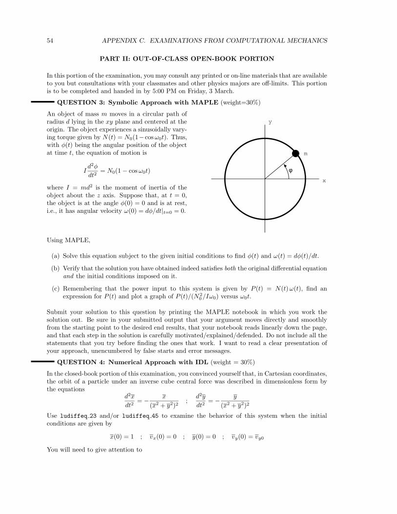
54 APPENDIX C. EXAMINATIONS FROM COMPUTATIONAL MECHANICS
PART II: OUT-OF-CLASS OPEN-BOOK PORTION
In this portion of the examination, you may consult any printed or on-line materials that are availableto you but consultations with your classmates and other physics majors are off-limits. This portionis to be completed and handed in by 5:00 PM on Friday, 3 March.
QUESTION 3: Symbolic Approach with MAPLE (weight=30%)
An object of mass m moves in a circular path ofradius d lying in the xy plane and centered at theorigin. The object experiences a sinusoidally vary-ing torque given by N(t) = N0(1−cos ω0t). Thus,with φ(t) being the angular position of the objectat time t, the equation of motion is
Id2φ
dt2= N0(1 − cos ω0t)
where I = md2 is the moment of inertia of theobject about the z axis. Suppose that, at t = 0,the object is at the angle φ(0) = 0 and is at rest,i.e., it has angular velocity ω(0) = dφ/dt|t=0 = 0.
x
y
φ
m
Using MAPLE,
(a) Solve this equation subject to the given initial conditions to find φ(t) and ω(t) = dφ(t)/dt.
(b) Verify that the solution you have obtained indeed satisfies both the original differential equationand the initial conditions imposed on it.
(c) Remembering that the power input to this system is given by P (t) = N(t)ω(t), find anexpression for P (t) and plot a graph of P (t)/(N 2
0 /Iω0) versus ω0t.
Submit your solution to this question by printing the MAPLE notebook in which you work thesolution out. Be sure in your submitted output that your argument moves directly and smoothlyfrom the starting point to the desired end results, that your notebook reads linearly down the page,and that each step in the solution is carefully motivated/explained/defended. Do not include all thestatements that you try before finding the ones that work. I want to read a clear presentation ofyour approach, unencumbered by false starts and error messages.
QUESTION 4: Numerical Approach with IDL (weight = 30%)
In the closed-book portion of this examination, you convinced yourself that, in Cartesian coordinates,the orbit of a particle under an inverse cube central force was described in dimensionless form bythe equations
d2x
dt2= − x
(x2 + y2)2;
d2y
dt2= − y
(x2 + y2)2
Use ludiffeq 23 and/or ludiffeq 45 to examine the behavior of this system when the initialconditions are given by
x(0) = 1 ; vx(0) = 0 ; y(0) = 0 ; vy(0) = vy0
You will need to give attention to

C.3. FINAL EXAMINATION – 15 MARCH 2006 55
• Creating the appropriate pro-file to define these equations for ludiffeq 23 or ludiffeq 45.
• Using (ludiffeq 23 and/or ludiffeq 45) and plot to generate the solution and a graph ofthe orbit for vy0 = 1 (which should produce a circular orbit) and for two other values of thisvelocity, one slightly larger than 1 and the other slightly smaller than 1. In each case, choosethe time interval over which you generate the solution wisely to show enough of the orbit toreveal its full character.
• Verifying that the solutions you ultimately accept are accurate at least to the resolution of thegraphs—and presenting evidence to support your contentions in this regard. Remember thatyou have both ludiffeq 23 and ludiffeq 45 at your disposal, that each of these routines hasa keyword tol, and that energy and angular momentum given in dimensionless form by
E = v2x + v2
y − 1
x2 + y2 ; L = x vy − y vx
are—or should be—conserved.
Submit your solution to this question by creating a LATEX document that includes (1) sufficientnarrative and sufficient sample IDL code to explain your approach and (2) the graphs associatedwith your presentation of your solution.
C.3 Final Examination – 15 March 2006
Physics 225: Computational Mechanics FINAL EXAMINATION 15 March 2006
This examination is a closed book examination, but reference to CPSUP is permitted and, unlessotherwise noted, calculators and integral tables are allowed. The examination is designed to takeno more than three hours. Each student is to answer Question 1 and any four of the remaining fivequestions (Questions 2, 3, 4, 5, and 6). In all cases, be sure to include enough narrative with eachsolution so that I can understand easily what you were thinking as you solved each problem. In thegrading, Question 1 will carry weight 3 and each of the remaining questions will carry weight 2.
Possibly useful information:
U = − Gm1m2
|r2 − r1|; U =
1
2kx2 ; U = mgz ; K =
1
2mv2 =
1
2Iω2
(1 + ε)q = 1 + qε + . . . ; MRCM =∑
i
miri ; W =
∫
F • dr
REMEMBER: You must answer Question 1.

56 APPENDIX C. EXAMINATIONS FROM COMPUTATIONAL MECHANICS
QUESTION 1: Gravitation; Small Amplitude Oscillations
x
y
aa
y MM
m
Two objects, each of mass M , are fixed on the x axis, one at x = +a and the other at x = −a.Another object of mass m is constrained to stay on the y axis but is free to move along that axis.
(a) Show that, when m is located at the point r = y j, the potential energy of m is given by
U(y) = − 2GMm
[a2 + y2]1/2
(Don’t work too hard. I am not asking you to evaluate an integral of the force, merely to usethe known potential energy of a mass near a second mass to construct the potential energy inthe present situation.) Were you to draw a graph of this function, I would hope you woulddeduce something like the graph at the end of this question. (Note that I did not ask you togenerate—or even defend—this graph.)
(b) Locate the one equilibrium point and classify it as stable or unstable on the basis of featuresof the potential energy.
(c) Find the y component of the force on m by evaluating an appropriate component of the gradientof the potential energy, and show that the equation of motion of m is
d2y
dt2= − 2GMy
(a2 + y2)3/2
(d) Examine the equation to which this equation of motion reduces when y � a, i.e., when y2 canbe ignored relative to a2, and determine the frequency of small amplitude oscillations aboutthe equilibrium point.
Now, if you introduce the dimensionless coordinates y = y/a and t =√
2GM/a3 t, you will find thatthe equation of motion becomes
d2y
dt2 = − y
(1 + y2)3/2
(Note that I did not ask you to deduce this form.)
(e) You wish to draw a graph of the position y of this object as a function of time t when y(0) = 1.0and vy(0) = 0. The ODE does not have an analytic solution, so you will have to invoke IDLand use a numerical method. Choose ludiffeq 23. Describe what you would do to

C.3. FINAL EXAMINATION – 15 MARCH 2006 57
• effect that solution,• obtain the desired graph, and• assess the accuracy of your solution.
In particular, be specific about the coding that you would use, both to define the ODE forIDL and to generate and plot the solution. Note: I am asking only how you would produce agraph on the workstation screen, not how you would produce hard copy of the graph.
REMEMBER: You are to answer any four of the remaining five questions.
QUESTION 2: A Projectile in a Strange Atmosphere
A projectile is fired from the origin with an initialvelocity v0 = vx0 i + vz0 k into a strange atmo-sphere in which air resistance acts only horizon-tally. The projectile thus experiences the forcesshown in the figure to the right. You may assumethat the projectile remains in the xz plane.
(a) Apply Newton’s second law to determine theequations of motion for this projectile.
z
x
mg
bvx
v0
(b) State the initial conditions to be imposed on the solution to the equations in part (a).
(c) Solve the equations obtained in part (a) subject to the initial conditions you identified inpart (b) to show that
x(t) =mvx0
b
(
1 − e−bt/m)
; z(t) = −1
2gt2 + vz0t

58 APPENDIX C. EXAMINATIONS FROM COMPUTATIONAL MECHANICS
(d) Explain briefly what is meant by the range of a projectile and then find an expression for therange of this projectile.
QUESTION 3: Orbits in Inverse Square Forces
In previous work, we have learned that a satellite of mass m orbiting a planet of mass M and radiusR is an ellipse characterized by eccentricity ε and constant angular momentum L. If we choose acoordinate system in which the force center is at the origin and the angle φ is measured from theperigee (point of closest approach), the radial coordinate ρ of the orbit is given as a function of φby the equation
ρ(φ) =L2/(m2GM)
1 + ε cos φ
where ε = 0 for a circular orbit and 0 < ε < 1 for elliptical orbits.
(a) For a general elliptical orbit, suppose that at perigee the speed of the satellite is vp and itsdistance from the force center is ρp.
i. Starting with the definition L = r × mv, show for that orbit that L = mvpρp.
ii. Using the result just obtained, show that,
ρ(φ)
R=
(
vp
vgraze
ρp
R
)2
1 + ε cos φ
where, as we have deduced in earlier work, vgraze =√
GM/R.
(b) Now, suppose a satellite is initially in the specific circular orbit of radius 4R. (Don’t overlookthe 4 .
i. By requiring the gravitational force to provide for the requisite centripetal acceleration,show that the speed of this satellite is given by vs = 1
2 vgraze.
ii. At a fateful instant, a very short but powerful burn of a rocket boosts the speed of thissatellite to 2
3 vgraze, thus putting the satellite into a new (elliptical) orbit whose perigeeis at the point where the boost was applied. Find
• the eccentricity ε of this new orbit.
• the radial coordinate of the new orbit at apogee (point of furthest distance from theforce center).
The first of these quantities will be a pure number; the second can be left as a multipleof R.
QUESTION 4: Center of Mass; Integration with MAPLE and IDL
A slender rod of length l (assume l > 0) lies along the x axis with one end at the origin and theother end at x = l. The rod carries a total mass M distributed non-uniformly with mass per unitlength λ(x) given at coordinate x by λ(x) = Ax2e−x/l. Remembering that
Rcm =1
M
∫
r dm
and taking M as a given (i.e., do not trouble to determine how A and M are related1),
1If you must know, A = M/[l3(2 − 5/e)].

C.3. FINAL EXAMINATION – 15 MARCH 2006 59
(a) Deduce an integral for the x coordinate Xcm of the center of mass of this rod.
(b) Describe how you would use MAPLE to evaluate the integral. Be specific about the state-ment(s) you would submit to MAPLE.
(c) Cast the integral in a dimensionless form and then describe how you would use luqsimp inIDL to evaluate it and assess the accuracy of your result. Be specific about the coding youwould use, both to define the integrand for IDL and to evaluate the integral once the integrandhas been defined.
QUESTION 5: The Lagrangian Approach
m m
k k’ k
x1 x2
In the text and in class, we found the equations of motion for the illustrated system by examiningthe forces experienced by the two blocks and invoking Newton’s second law. This problem leads youthrough an alternate, simultaneously mysterious and wondrous, way to deduce these same equationsfrom a starting point that focuses on energy rather than on forces. Take the table to be horizontal andfrictionless, let the springs be neither stretched nor compressed when the system is in equilibrium,and let the state of the system be described by the coordinates x1(t) and x2(t), which measure thepositions of the blocks from their equilibrium positions, and the velocities x1(t) and x2(t). Usingthe symbols x1, x2, x1 and x2,
• write down the kinetic energy K of the system.
• write down the potential energy U of the system.
• evaluate the Lagrangian L defined by L = K − U of the system.
• pretending—this is the mysterious part—that x1, x2, x1 and x2 are independent of one another,evaluate the quantities
∂L∂x1
and∂L∂x1
• finally, admitting that the positions and velocities are time dependent, evaluate
d
dt
(
∂L∂x1
)
− ∂L∂x1
= 0
and marvel at the result. (Done correctly, this process will lead you to the equation of motion forblock 1 without the hassle of figuring out the forces and making sure that all of them have beentaken into account!)
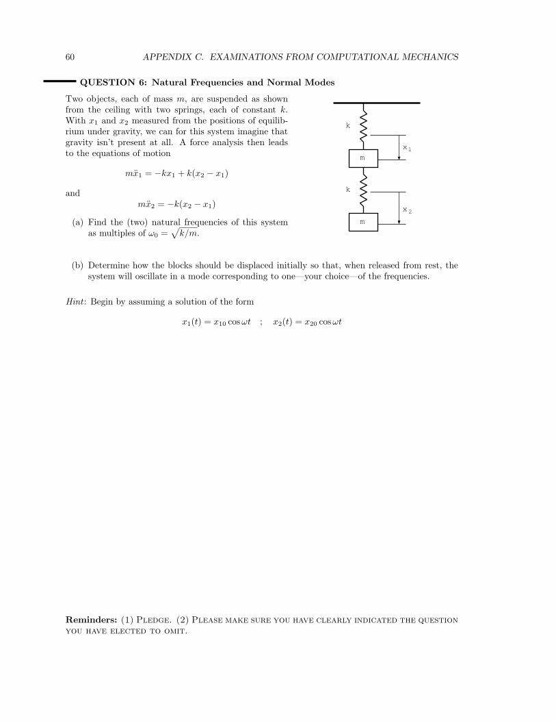
60 APPENDIX C. EXAMINATIONS FROM COMPUTATIONAL MECHANICS
QUESTION 6: Natural Frequencies and Normal Modes
Two objects, each of mass m, are suspended as shownfrom the ceiling with two springs, each of constant k.With x1 and x2 measured from the positions of equilib-rium under gravity, we can for this system imagine thatgravity isn’t present at all. A force analysis then leadsto the equations of motion
mx1 = −kx1 + k(x2 − x1)
andmx2 = −k(x2 − x1)
(a) Find the (two) natural frequencies of this systemas multiples of ω0 =
√
k/m.
k
k
m
m
x1
x2
(b) Determine how the blocks should be displaced initially so that, when released from rest, thesystem will oscillate in a mode corresponding to one—your choice—of the frequencies.
Hint : Begin by assuming a solution of the form
x1(t) = x10 cos ωt ; x2(t) = x20 cosωt
Reminders: (1) Pledge. (2) Please make sure you have clearly indicated the questionyou have elected to omit.

Appendix D
Options for Projects inComputational Physics
Each of Assignment 3 covering finite difference methods and Assignment 6 covering finite elementmethods in Physics 540 contains a small number of problems to be solved by everyone in the classand one assigned project for each student. Completion of each of these assignments involves
• reading appropriate sections in the text to learn about the method covered in the assignment,
• solving and writing out solutions to one or two exercises common to the entire class,1
• with respect to the assigned “big” exercise, putting a special effort into
◦ generating a solution and
◦ writing a carefully written document that
– describes in some detail how the problem was set up and solved (including a discussionof any particular wrinkles that had to be addressed),
– defending the accuracy of the solution,
– exploring the solution in as many creative ways as possible and, in particular, as afunction of any parameters—if any—in the exercise,
– making any other comments that seem appropriate, and
– discussing the features of the solution and its dependence on the parameters, and
• preparing a 15-minute oral summary of the solution and its properties and delivering thatsummary in class.
The problems that are assigned to individual students for each of these two assignments are tabulatedin Sections D.1 and D.2, respectively.
Assignment 7 contains only a project, this time of the student’s choice but subject to theinstructor’s approval. Students spend about three weeks working on this project, which can involveany of the techniques addressed during the term but must be substantial and challenging. Thehandout describing this assignment is presented in Section D.3.
1On Assignment 3, the two common exercises involve (a) modifying a template discussed in the text to solve a1D ODE and (b) adding a convergence test to a program for solving Laplace’s equation. On Assignment 6, the onecommon exercise involves using a commercial finite element program to find the electrostatic potential and chargedistributions in an annular region with Dirichlet boundary conditions at both the inner and outer radii.
61

62 APPENDIX D. OPTIONS FOR PROJECTS IN COMPUTATIONAL PHYSICS
a b
cd
ef
g
Figure D.1: Diagram for Big Exercise B1.1 and B1.2.
D.1 Big Exercise #1 (Assignment 3)
Each student will be assigned one of the following problems as a component of Assignment 3. Shouldthe course sometime enroll more than six students, additional problems will be found.
B1.1 A two-dimensional plate is made by taking a square of side 1 unit and cutting a square ofside 0.5 unit out of one corner as shown in Fig. D.1. Suppose the temperature along sidesaf and ab is maintained at 0 ◦C, the temperature increases linearly from 50 ◦C at e and at cto 100 ◦C at d, and sides fe and bc are insulated. If the entire plate is initially at 0 ◦C, useLSODE to study the approach of the temperature to equilibrium and, in particular, determinethe equilibrium temperature.
B1.2 Consider a thin membrane stretched over the frame shown in Fig. D.1. Introduce a coordinatesystem in which the point a defines the origin and the lines ab and af—each of unit length—liealong the x and y axes, respectively. In the chosen coordinates, the point d has coordinates( 12 , 1
2 ). Suppose this membrane to be drawn aside from the plane of the paper so that therectangle gdcba is undisplaced and the square gdfe assumes a shape given by u(x, y, 0) =64x( 1
2 − x)(y − 12 )(1 − y). Suppose further that this membrane is then released from rest.
Use LSODE to study the subsequent motion of the membrane. In particular, obtain surfaceplots of the shape of the membrane over the xy plane for enough different times to make thecharacter of the motion clear. Remember that, in a dimensionless presentation, the motion ofthe membrane satisfies the two-dimensional wave equation
∂2u
∂t2=
∂2u
∂x2+
∂2u
∂y2
B1.3 Suppose a quantum particle of mass m is initially in the state
Ψ(x, 0) =1
√
a√
πe−(x+5a)2/2a2
eik0x
which represents a particle (1) whose wave function initially is Gaussian with a width on theorder of a centered at x = −5a and (2) the expectation value of whose momentum is hk0 and—assuming non-relativistic motion—(3) the expectation value of whose velocity is v0 = hk0/m.Suppose also that the particle moves under the influence of a static potential energy given by
V (x) =
0 x < −a
1
2V0
(
1 + cosπx
a
)
−a ≤ x ≤ a
0 x > a
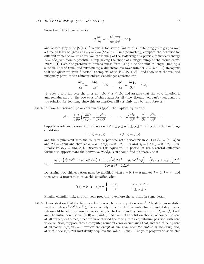
D.1. BIG EXERCISE #1 (ASSIGNMENT 3) 63
Solve the Schrodinger equation,
ih∂Ψ
∂t= − h2
2m
∂2Ψ
∂x2+ V Ψ
and obtain graphs of |Ψ(x, t)|2 versus x for several values of t, extending your graphs overa time at least as great as tend = 2x0/(hk0/m). Time permitting, compare the behavior fordifferent values of k0. In effect, you are looking at the scattering of a particle of incident energyE = h2k0/2m from a potential hump having the shape of a single hump of the cosine curve.Hints: (1) Cast the problem in dimensionless form using a as the unit of length, finding asuitable unit of time, and introducing a dimensionless wave number k = k0a. (2) Recognizethat the quantum wave function is complex, write Ψ = Ψr + iΨi, and show that the real andimaginary parts of the (dimensionless) Schodinger equation are
∂Ψr
∂t= −∂2Ψi
∂x2+ V Ψi ;
∂Ψi
∂t=
∂2Ψr
∂x2− V Ψi
(3) Seek a solution over the interval −10a ≤ x ≤ 10a and assume that the wave function isand remains zero at the two ends of this region for all time, though you can’t then generatethe solution for too long, since this assumption will certainly not be valid forever.
B1.4 In (two-dimensional) polar coordinates (ρ, φ), the Laplace equation is
∇2u =1
ρ
∂
∂ρ
(
ρ∂u
∂ρ
)
+1
ρ2
∂2u
∂φ2= 0 =⇒ ρ2 ∂2u
∂ρ2+ ρ
∂u
∂ρ+
∂2u
∂φ2= 0
Suppose a solution is sought in the region 0 < a ≤ ρ ≤ b, 0 ≤ φ ≤ 2π subject to the boundaryconditions
u(a, φ) = f(φ) ; u(b, φ) = g(φ)
and the requirement that the solution be periodic with period 2π in φ. Let ∆ρ = (b − a)/nand ∆φ = 2π/m and then let ρi = a + i∆ρ, i = 0, 1, 2, . . . , n and φj = j ∆φ, j = 0, 1, 2, . . . ,m.Finally let ui,j = u)ρi, φj). Discretize this equation. In particular use a central differenceformula to approximate the derivative ∂u/∂ρ. You should find ultimately that
ui,j =ui+1,j
(
ρ2i ∆φ2 + 1
2ρi ∆φ2 ∆ρ)
+ ui−1,j
(
ρ2i ∆φ2 − 1
2ρi ∆φ2 ∆ρ)
+(
ui,j+1 + ui,j−1
)
∆ρ2
2 ρ2i ∆φ2 + 2∆ρ2
Determine how this equation must be modified when i = 0, i = n and/or j = 0, j = m, andthen write a program to solve this equation when
f(φ) = 0 ; g(φ =
{
−100 −π < φ < 0
100 0 ≤ φ ≤ π
Finally, compile, link, and run your program to explore the solution in some detail.
B1.5 Demonstration that the full discretization of the wave equation u = c2u′′ leads to an unstablemethod unless c2 ∆t2/∆x2 ≤ 1 is extremely difficult. To illustrate this the instability, recastfdmwave1d to solve the wave equation subject to the boundary conditions u(0, t) = u(l, t) = 0and the initial conditions u(x, 0) = 0, ∂u(x, 0)/∂x = 0. The solution should, of course, be zeroat all subsequent times, since we have started the string in its equilibrium position with zerovelocity. Now, suppose that a computer-roundoff error occurs such that, instead of being zeroat all nodes, u(x,∆t) = 0 everywhere except at one node near the middle of the string and,at that node u(x,∆t) mistakenly acquires the value 1 (one). Use your program to solve this

64 APPENDIX D. OPTIONS FOR PROJECTS IN COMPUTATIONAL PHYSICS
problem for choices of the parameters that make α = 0.5 and other choices that make α = 1.5.Look at the solution with print or plot frequency 1 and compare the way in which that onedisruption of a value at the end of the first time step propagates forward in time for the twovalues of α.
B1.6 Demonstration that the full discretization of the diffusion equation u = α2u′′ leads to anunstable method unless α2 ∆t/∆x2 ≤ 1/2 is extremely difficult. To illustrate this instability,recast fdmdiffus1d to solve the diffusion equation subject to the boundary conditions u(0, t) =u(l, t) = 0 and the initial condition u(x, 0) = 0. The solution should, of course, be zero atall subsequent times, since we have started the temperature distribution with its equilibriumvalues. Now, suppose that a computer-roundoff error occurs such that, instead of being zero atall nodes, u(x,∆t) = 0 everywhere except at one node near the middle of the rod and, at thatnode u(x,∆t) mistakenly acquires the value 1 (one). Use your program to solve this problemfor choices of the parameters that make γ = 0.25 and other choices that make γ = 1.0. Look atthe solution with print or plot frequency 1 and compare the way in which that one disruptionof a value at the end of the first time step propagates forward in time for the two values of γ.
D.2 Big Exercise #2 (Assignment 6)
Each student will be assigned one of the following problems as a component of Assignment 6. Shouldthe course sometime enroll more than six students, additional problems will be found.
B2.1 Suppose a linear element e is characterized by three nodes at x(e)1 , x
(e)2 , and x
(e)3 . Further, let
the solution ϕ(e) on that element be approximated by the quadratic function
ϕ(e) = a(e) + b(e)x + c(e)x2
(a) Find the constants a(e), b(e), and c(e) that will make this function match the specific values
ϕ(e)1 , ϕ
(e)2 , and ϕ
(e)3 at the points x = x
(e)1 , x
(e)2 , and x
(e)3 , respectively. (b) Substituting these
values into the above expression and grouping terms appropriately, cast the result in the form
ϕ(e) =3
∑
i=1
ϕ(e)i N
(e)i (x)
and show that the shape functions N(e)i (x) appropriate to this three-noded linear element are
N(e)1 (x) =
1
∆
∣
∣
∣
∣
∣
∣
∣
1 x x2
1 x(e)2 (x
(e)2 )2
1 x(e)3 (x
(e)3 )2
∣
∣
∣
∣
∣
∣
∣
=(x
(e)2 − x)(x
(e)3 − x)
(x(e)2 − x
(e)1 )(x
(e)3 − x
(e)1 )
N(e)2 (x) =
1
∆
∣
∣
∣
∣
∣
∣
∣
1 x(e)1 (x
(e)1 )2
1 x x2
1 x(e)3 (x
(e)3 )2
∣
∣
∣
∣
∣
∣
∣
=(x − x
(e)1 )(x
(e)3 − x)
(x(e)2 − x
(e)1 )(x
(e)3 − x
(e)2 )
N(e)3 (x) =
1
∆
∣
∣
∣
∣
∣
∣
∣
1 x(e)1 (x
(e)1 )2
1 x(e)2 (x
(e)2 )2
1 x x2
∣
∣
∣
∣
∣
∣
∣
=(x − x
(e)1 )(x − x
(e)2 )
(x(e)3 − x
(e)1 )(x
(e)3 − x
(e)2 )
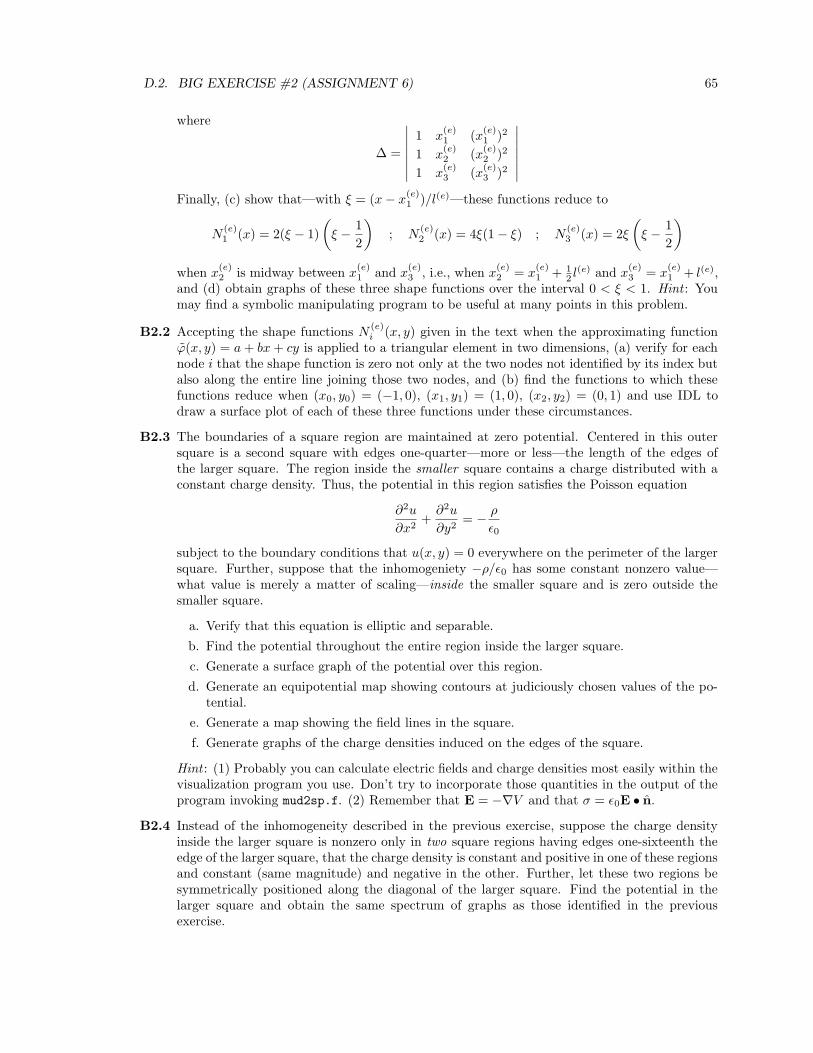
D.2. BIG EXERCISE #2 (ASSIGNMENT 6) 65
where
∆ =
∣
∣
∣
∣
∣
∣
∣
1 x(e)1 (x
(e)1 )2
1 x(e)2 (x
(e)2 )2
1 x(e)3 (x
(e)3 )2
∣
∣
∣
∣
∣
∣
∣
Finally, (c) show that—with ξ = (x − x(e)1 )/l(e)—these functions reduce to
N(e)1 (x) = 2(ξ − 1)
(
ξ − 1
2
)
; N(e)2 (x) = 4ξ(1 − ξ) ; N
(e)3 (x) = 2ξ
(
ξ − 1
2
)
when x(e)2 is midway between x
(e)1 and x
(e)3 , i.e., when x
(e)2 = x
(e)1 + 1
2 l(e) and x(e)3 = x
(e)1 + l(e),
and (d) obtain graphs of these three shape functions over the interval 0 < ξ < 1. Hint : Youmay find a symbolic manipulating program to be useful at many points in this problem.
B2.2 Accepting the shape functions N(e)i (x, y) given in the text when the approximating function
ϕ(x, y) = a + bx + cy is applied to a triangular element in two dimensions, (a) verify for eachnode i that the shape function is zero not only at the two nodes not identified by its index butalso along the entire line joining those two nodes, and (b) find the functions to which thesefunctions reduce when (x0, y0) = (−1, 0), (x1, y1) = (1, 0), (x2, y2) = (0, 1) and use IDL todraw a surface plot of each of these three functions under these circumstances.
B2.3 The boundaries of a square region are maintained at zero potential. Centered in this outersquare is a second square with edges one-quarter—more or less—the length of the edges ofthe larger square. The region inside the smaller square contains a charge distributed with aconstant charge density. Thus, the potential in this region satisfies the Poisson equation
∂2u
∂x2+
∂2u
∂y2= − ρ
ε0
subject to the boundary conditions that u(x, y) = 0 everywhere on the perimeter of the largersquare. Further, suppose that the inhomogeniety −ρ/ε0 has some constant nonzero value—what value is merely a matter of scaling—inside the smaller square and is zero outside thesmaller square.
a. Verify that this equation is elliptic and separable.
b. Find the potential throughout the entire region inside the larger square.
c. Generate a surface graph of the potential over this region.
d. Generate an equipotential map showing contours at judiciously chosen values of the po-tential.
e. Generate a map showing the field lines in the square.
f. Generate graphs of the charge densities induced on the edges of the square.
Hint : (1) Probably you can calculate electric fields and charge densities most easily within thevisualization program you use. Don’t try to incorporate those quantities in the output of theprogram invoking mud2sp.f. (2) Remember that E = −∇V and that σ = ε0E • n.
B2.4 Instead of the inhomogeneity described in the previous exercise, suppose the charge densityinside the larger square is nonzero only in two square regions having edges one-sixteenth theedge of the larger square, that the charge density is constant and positive in one of these regionsand constant (same magnitude) and negative in the other. Further, let these two regions besymmetrically positioned along the diagonal of the larger square. Find the potential in thelarger square and obtain the same spectrum of graphs as those identified in the previousexercise.

66 APPENDIX D. OPTIONS FOR PROJECTS IN COMPUTATIONAL PHYSICS
100
0
50
50
Figure D.2: Geometry for Exercise B2.5.
B2.5 Find the steady state temperature distribution in the geometry shown in Fig. D.2. All arcsare semicircles or quarter-circles of radius 1 unit, and the straight patches are either 2 or 4units in length. As indicated by the shading, the straight patches are insulated. Each circulararc is maintained at the indicated temperature in degrees Celsius. Assume that the materialof which the shape is constructed has uniform thermal conductivity and heat capacity.
B2.6 Find the electrostatic potential in the geometry of Fig. D.3 when the large semicircle andthe diameter are maintained at 0 Volts and the region inside the inner circle contains electriccharge distributed uniformly with density 1 C/m2. Note that you will need to mesh the areainside the inner circle as well as the area between the inner circle and the outer boundary of theregion of interest, but you must do so in a way that preserves the nodes along the inner circle.To specify the charge density, you will have to provide a “boundary condition” on and withinthat inner circle. I think—but I am not sure—that you want to migrate from the Main menuthrough the Boundary Conditions menu to the Electrostatic menu from the ‘BoundaryCondition Class’ panel in the Boundary Conditions menu. The ‘Face Charge’ button inthat menu may be the one you want in order to apply a distributed charge to a selection offaces.
D.3 Big Exercise #3 (Assignment 7)
Your last obligation—there is no final examination—to Physics 540 is to complete an extendedproject of your choice (but subject to my approval), present an oral report on that project in thelast week of the term, and hand in a carefully written paper on the project by noon on Saturday atthe end of the term. A brief written project proposal is due at the beginning of week 7. I offer thefollowing suggestions to stimulate your thinking about this project. I am, of course, willing to listento—and to help refine—any other proposals that you might have.
B3.1 The normal modes of oscillation of a square membrane. This problem can be approachedby using finite difference methods to generate an equivalent matrix eigenvalue problem and

D.3. BIG EXERCISE #3 (ASSIGNMENT 7) 67
x
y
-1.0 1.0-0.3
0.35
V = 0
V = 100
Figure D.3: Geometry for Problem B2.6.
then solving that problem numerically to obtain both the lowest several eigenvalues (naturalfrequencies) and the shapes of the membrane in each mode. This exercise would involve writingyour own IDL or FORTRAN code to implement the numerical solution, though you would wantto find and use IDL routines or Numerical Recipes routines for the actual solution once youhave set up the matrix whose eigenvalues and eigenvectors are to be found.
B3.2 A three-dimensional electrostatic problem in Cartesian coordinates whose solution would in-volve using the multigrid subroutine mud3sp.f.
B3.3 The two-dimensional Laplace equation in cylindrical coordinates with some choice (or choices)of boundary conditions. This problem would be approached using the multigrid subroutinemud2sp.f, though care would be needed to set up the problem in non-Cartesian coordinates.
B3.4 The temperature distribution inside a three-dimensional region that is cylindrically symmetric.This exercise should be doable with mud2sp.f, though care would be needed to set up theproblem in non-Cartesian coordinates.
B3.5 The normal modes of oscillation of an irregularly shaped two-dimensional membrane, whichwould involve learning about some features of MARC/MENTAT not discussed in class.
B3.6 A situation using MARC/MENTAT to set up and solve a problem in a fairly simple three-dimensional geometry.

68 APPENDIX D. OPTIONS FOR PROJECTS IN COMPUTATIONAL PHYSICS

Bibliography
[1] NEdit is a text editor available under a GNU General Public License. Information is availableat the website http://www.nedit.org.
[2] XEmacs is a text editor available under a GNU General Public License. Information is availableat the website http://www.xemacs.org.
[3] Excel is a component of the Microsoft Office suite and is available for purchase from MicrosoftCorporation. Information is available at the website http://office.microsoft.com/en-us.
[4] IDL is a program for array processing and graphical visualization and is available for purchasefrom ITT Industries. Information is available at the website http://www.ittvis.com.
[5] MATLAB is a program for array processing and graphical visualization and is avail-able for purchase from The MathWorks. Information is available at the websitehttp://www.mathworks.com.
[6] OCTAVE is a program for array processing and graphical visualization and is available under aGNU General Public License. Its syntax is similar to that of MATLAB. Information is availableat the website http://www.octave.org.
[7] MAPLE is a computer algebra system and is available for purchase from Waterloo Software.Information is available at the website http://www.maplesoft.com.
[8] Mathematica is a computer algebra system and is available for purchase from Wolfram Research.Information is available at the website http://www.wolfram.com.
[9] MAXIMA is a computer algebra system and is available under a GNU General Public License.Its syntax is similar to the no-longer-available commercial program MACSYMA. Informationis available at http://maxima.sourceforge.net.
[10] Kaleidagraph is a program for generating publication-quality graphs and is available for purchasefrom Synergy Software. Information is available at the website http://www.synergy.com.
[11] The Numerical Recipes library of FORTRAN and C subroutines is available for purchase fromNumerical Recipes Software. Information is available at the website http://www.nr.com.
[12] ODEPACK is a package containing numerous FORTRAN solvers for ODEs, of which LSODE(the Livermore Solver for ODEs) is a component. This package is in the public domain. Infor-mation is available at the website www.netlib.org.
[13] MUDPACK is a package containing numerous FORTRAN solvers for elliptic partial differentialequations in two and three dimensions. This package is in the public domain. Information isavailable at the website http://www.scd.ucar.edu/css/software/mudpack.
69

70 BIBLIOGRAPHY
[14] Multisim 7 is a program for circuit simulation and is available for purchase from ElectronicsWorkbench Corporation. Information about the product and the appropriate local offices of thecompany is available at the website http://www.electronicsworkbench.com.
[15] SPICE is a program for simulating the behavior of electric circuits and is available for purchaseat nominal cost. For information, start at www.berkeley.edu and search for SPICE.
[16] LabView is a program for designing and executing software to access laboratory equipment foron-line acquisition of data. It is available for purchase from National Instruments Corporation.Information is available from the website http://www.NI.com/labview.
[17] LATEX is freely available for many platforms via ftp download from several archives around theworld. For information, start at www.tug.org.
[18] Tgif is a program for drawing assorted diagrams and writing those descriptions in files of severaldifferent types. For information, go to www.ucla.edu and search for Tgif.
[19] PowerPoint is a component of the Microsoft Office suite and is available forpurchase from Microsoft Corporation. Information is available at the websitehttp://office.microsoft.com/en-us.
[20] LoggerPro is the software that interfaces with LabPro hardware to connect a laboratory com-puter to assorted digital sensors. This software and the associated hardware are availablefor purchase from Vernier Software and Technology. Information is available at the websitehttp://www.vernier.com.
[21] Praat is freely available software for Fourier analysis—more broadly phonetics—of digitallyrecorded sound waves. Information is available at the website http://www.praat.org.
[22] SpaceTime is software for simulating time dilation, length contraction, and other special rela-tivistic phenomena. It is available for purchase from Physics Academic Software. Informationis available at the website http://www.webassign.net/pas.
[23] MARC/MENTAT is a pair of programs for setting up and solving partial differential equa-tions by finite element techniques and is available for lease from MSC Software. Information isavailable at the website http://www.mscsoftware.com.