i

Table of Content List of figures ................................................................................................................................... i

List of tables .................................................................................................................................... ii

Acronyms ........................................................................................................................................ ii

Justification ..................................................................................................................................... 1

Previous publications ...................................................................................................................... 2

Objectives ....................................................................................................................................... 4

Methodology ................................................................................................................................... 5

Governing equations ................................................................................................................... 5

Channel networks........................................................................................................................ 8

Lateral weir design .................................................................................................................... 12

Inverted syphon design ............................................................................................................. 14

Sluice gates design .................................................................................................................... 16

Numerical solution of system ................................................................................................... 17

Preliminary results .................................................................................................................... 18

References ..................................................................................................................................... 20

List of figures

Figure 1: Definition sketches for the governing sketches. .............................................................. 6

Figure 2: Example of a looped channel network. ........................................................................... 9

Figure 3: Definition sketch of a channel junctions in a looped network. ..................................... 12

Figure 4: Cross section of a suppressed rectangular weir. ............................................................ 13

Figure 5: Example of a siphon profile that crosses a road. ........................................................... 15

Figure 6: Sluice gate definition sketch.......................................................................................... 17

Figure 7: Case study of a looped channel network with lateral weirs. ......................................... 18

Figure 8: Percent of error for reach length of both method results for the case study of the looped

channel network. ........................................................................................................................... 20

ii

List of tables

Table 1: Geometric and roughness properties of the channel system ........................................... 19

Acronyms

BiCGSTAB Bi-Conjugated Gradient Stabilizer with Preconditioner Method

DSM Direct Step Method

GVF Gradually-Varied Flow

HEC-RAS Hydrologic Engineering Center- River Analysis System

iLU incomplete LU factorization

PR Puerto Rico

StdSM Standard Step Method

SSM Simultaneous Solution Method

UDT Utah Department of Transportation

1

Justification

The first major irrigation system was built during Egypt’s First Dynasty, close to 3100 B.C.

as a diversion of flood waters of the Nile River [1]. Irrigation canals transport water from a source,

such as a natural river or a reservoir, to a crop field or a community. Irrigation canals are vital for

agriculture. One-sixth of irrigated crop land produces one-third of the world’s harvest of food

crops [2]. Food production is a global concern in a world of growing population and limited

resources. Sustainability of food production depends on sound and efficient water use and

conservation practices consisting mainly of irrigation development and management [3]. It is of

upmost importance for farmers to control the water distribution in irrigation systems. Hydraulic

structures such as weirs and gates must be set at specific levels to distribute the correct amount of

water for crop production and water conservation.

This research will develop a computer model to determine the water levels and discharges

in complex irrigation channel networks including hydraulic structures to control water distribution.

This computer model will provide farmers information on flow levels and volumetric discharges,

helping then to make decisions on irrigation water for their crops. The agricultural community will

be able to apply of water conservation and management more efficiently. The scope of research

will be to model irrigation channel networks that may be composed of several channel branches

and loops. The research will be limited to subcritical flow conditions on the channel system.

Analysis and/or design of hydraulic structures in irrigation system, such as lateral weirs, gates and

inverted syphons, will be included. The design computer tool will have the capacity of modeling

any channel configuration, including series, parallel and network channel systems and solve for

flow and water levels simultaneously.

Hydraulic structures are an essential component in real-life scenarios of irrigation channels.

An example of a hydraulic engineering applications is the Lajas Valley Irrigation System, located

on the southwest of Puerto Rico (PR). This system has an annual discharge of 30,830 acre-ft of

water supply for agriculture and potable water supply. Also, it provides irrigation water to 330

intakes and four water treatments plants. This system impacts approximately 100,000 people in its

high season of tourism and vacation periods [4]. Irrigation districts are vital for sustainability in

Puerto Rico and other countries.

2

Previous publications

Gradually varied flow (GVF) has been studied and researched since 19th century.

Chaudhry and Schulte [5] were one of the first pioneers to develop an algorithm for parallel

channels in 1986. Their algorithm solve for water depths and discharges at different sections for

steady-state and GVF conditions based on two fundamental equations: energy equation and

continuity equation. The nonlinear matrix system is solved simultaneously using the Newton-

Raphson method. In order to increase accuracy, and reduce computer time and storage, they found

a way to transform the resulting Jacobian matrix into a banded matrix for series and parallel

channels. In a similar manner, Chaudhry and Schulte [6] extended their previous algorithm to solve

GVF conditions in a channel network, however, the matrix became sparse and more difficult to

solve. This channel network algorithm is based on the same methodology as the parallel-channel

algorithm; but can solve for multiple channel configurations, such as series, parallel and networks.

The two models were applied to an idealized channel network. Results were compared with those

obtained by the fourth-order Runge-Kutta method for each channel configuration, which were

almost identical as described by the author.

A decade after the publication of Chaudhry and Schulte algorithm, Naidu et. al. [7]

presented an algorithm for GVF computations in tree-type channel networks. This algorithm

computes the water surface profile under the same flow conditions as Chaudhry and Schulte. The

solving technique for this algorithm decomposes the channel network into smaller units that are

solve using the fourth-order Runge-Kutta method, and connects all the solutions using the

Shooting Method. This technique does not involve solving simultaneously a large matrix system;

opposite to the one presented by Chaudhry and Schulte. The model was applied to an idealized

tree-type channel network as Chaudhry and Schulte study. Their algorithm was more efficient than

the direct method using the Newton-Raphson technique by an order of magnitude.

Reddy and Bhallamudi [8] developed an algorithm to compute water surface profiles in

steady, GVF of channel networks. Their algorithm computes the same two variables as Chaudhry

and Schulte; flow depths and discharges at a cyclic looped channel network. Although Reddy and

Bhallamudi’s algorithm is very similar to the one from Chaudhry and Schulte, their solving

methodology is very different. Reddy and Bhallamudi’s algorithm is based on three principles:

classifies the computations in an individual channel as an initial value problem or a boundary value

3

problem; determines the path for linking the solution from individual channels; and the Netwon-

Raphson iterative technique is used for obtaining the network solution [8]. Therefore, this

algorithm does not have to solve large matrix systems. The model was tested with the idealized

channel network presented in Chaudhry and Schulte, and Naidu et. al. study. The efficiency of

their algorithm compared with Naidu et. al [7] technique.

Sen and Garg [9] developed a model for unsteady flow in channel networks using St.

Venant equations. Sen and Garg’s algorithm uses the finite difference method to solve the system

of equations for all branches of the network simultaneously. The algorithm does not require any

special node numbering schemes. The number of equations to be solved reduce to four times the

number of branches in the network, resulting in a significant reduction in storage requirements and

solution time. The model was applied to two idealized channel networks, one looped network and

one branch network.

In a different manner, Islam et al. [10] conducted a comparison of two channel network

algorithms. The two algorithms had different techniques for separating end-node variables for each

branch; forward-elimination and branch-segment transformation equation. Both algorithms model

steady and unsteady flows in branched and looped channel networks. The St. Venant equations are

discretized using the four-point implicit Preissmann scheme and the nonlinear matrix system is

solved using the Newton-Raphson method. The model was applied to similar channel networks as

Sen and Garg. Islam et al. [10] concludes that the algorithm that uses the branch-segment

transformation equation is found to be at least five times faster and require less computer storage

than the algorithm using forward-elimination method. In a similar manner, Islam et al. [11]

extended his previous work and developed a hydraulic simulation model for irrigation channel

networks. The model uses the same discretization technique for the St. Venant equations, as his

previous work; but solves the nonlinear matrix system using the sparse matrix solution techniques.

Similarly, this algorithm models the same flow conditions and channel configuration as its

previous algorithm. In addition, this algorithm is capable of simulating different boundary

conditions; such as discharge and stage hydrographs, rating curves, and uniform flow. At the

moment of this research, Islam et al. [11] study was the only algorithm that include the analysis of

different hydraulic structures; such as weirs, sluice gates, drops/falls, pipe outlet, and imposed

discharge. Also, it was the only algorithm to include a user friendly graphical user interface for

entering and editing channel network description and boundary conditions. Even though Islam et

4

al. affirms that its algorithm is capable of solving complex channel networks, the results presented

were only for a simple network of four channels connected in series from the Kangsabati irrigation

project at West Bengal, India. Their results were similar to the ones from a HEC-RAS model and

performed satisfactory for most of the irrigation event at the irrigation project. This case does not

represent a challenging example for other solutions procedures.

At the beginning of this decade, Zhu et al. [12] develop an algorithm for gradually-varied

subcritical flow in channel networks. This algorithm simulates the same flow conditions as Islam

et al. [11] and Sen and Garg’s [9] algorithm; and solves the system using the same techniques as

Islam et al. [11] first algorithm. The algorithm treats backwater effects at the junction points on

the basis of junction-point water stage prediction and correction. The model was applied to two

hypothetical channel networks and a real-life river network in South China, in which the simulated

results compared well with ones from literature and measurements.

Objectives

The main objective for this research is to develop a computer model to determine discharge

and water levels in complex irrigation channel networks including hydraulic structures to control

water distribution. The solution algorithm will solve the mass and energy equation for GVF plus

additional equations to analyze and/or design lateral weir, sluiced gates and inverted syphons. To

the research knowledge, the addition of analysis and/or design of hydraulic structures for irrigation

systems as part of a simultaneous solution has not been proposed before. As part of this research,

the following tasks will be completed:

1. Development of a computer algorithm: The software will be able to solve a wide variety

of configurations of irrigation canals (series, parallel or network systems), including

design and/or analysis of hydraulic structures commonly found in such systems (lateral

weir, sluiced gates and inverted syphons).

2. Development of a graphical user interface (GUI): The GUI will allow a user friendly

interaction with the numerical model.

3. Model application: The new tool will be used in a case study. Efforts will be made to

collect information of “Arenal Tempisque” irrigation district located in Guanacaste,

Costa Rica. This is a major irrigation project for crop production in this Central

5

American country. The system if formed by three irrigation sub-districts with a total of

eighty-nine irrigation channels. Dr. Alejandra Rojas from the Department of

Agricultural Engineering of the University of Costa Rica (UCR) has collaborated

previously with the chairman of this research. Access to field data and new data

measurements could be granted through this partnership.

Methodology

This section consists on describing the proposed methodology for the proposal. First, the

governing equations of the gradually varied flow in open channel will be presented with its

assumptions. Second, the system of equations for the channel network will be proposed with the

boundary conditions of the system. Third, design of some of the hydraulic structures that might be

present on the channel network will be discuss. This include the design of lateral weir, inverted

syphon and sluice gates. The numerical method selected for the solution of the system will be

discuss in more detail. Finally, some preliminary results from a case study of a looped channel

network will be presented.

Governing equations

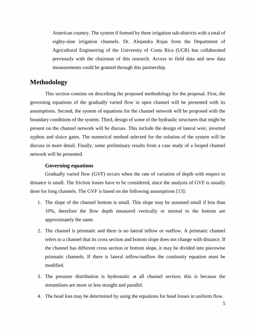
Gradually varied flow (GVF) occurs when the rate of variation of depth with respect to

distance is small. The friction losses have to be considered, since the analysis of GVF is usually

done for long channels. The GVF is based on the following assumptions [13]:

1. The slope of the channel bottom is small. This slope may be assumed small if less than

10%, therefore the flow depth measured vertically or normal to the bottom are

approximately the same.

2. The channel is prismatic and there is no lateral inflow or outflow. A prismatic channel

refers to a channel that its cross section and bottom slope does not change with distance. If

the channel has different cross section or bottom slope, it may be divided into piecewise

prismatic channels. If there is lateral inflow/outflow the continuity equation must be

modified.

3. The pressure distribution is hydrostatic at all channel section; this is because the

streamlines are more or less straight and parallel.

4. The head loss may be determined by using the equations for head losses in uniform flow.

6

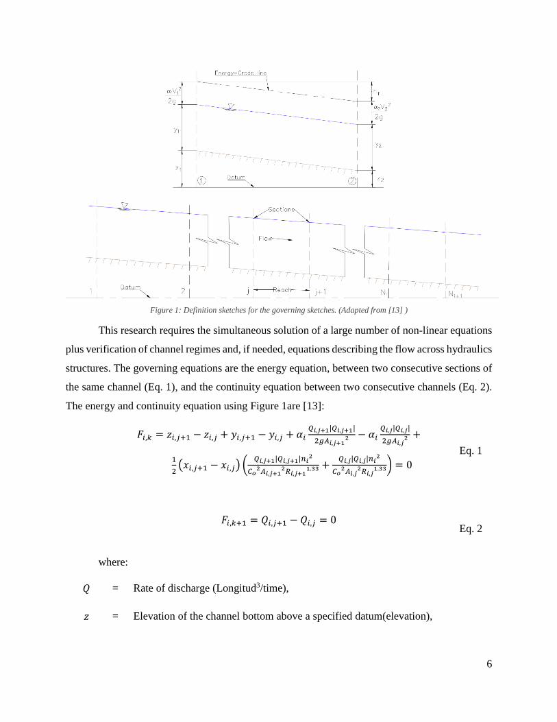
Figure 1: Definition sketches for the governing sketches. (Adapted from [13] )

This research requires the simultaneous solution of a large number of non-linear equations

plus verification of channel regimes and, if needed, equations describing the flow across hydraulics

structures. The governing equations are the energy equation, between two consecutive sections of

the same channel (Eq. 1), and the continuity equation between two consecutive channels (Eq. 2).

The energy and continuity equation using Figure 1are [13]:

𝐹𝑖,𝑘 = 𝑧𝑖,𝑗+1 − 𝑧𝑖,𝑗 + 𝑦𝑖,𝑗+1 − 𝑦𝑖,𝑗 + 𝛼𝑖𝑄𝑖,𝑗+1|𝑄𝑖,𝑗+1|

2𝑔𝐴𝑖,𝑗+12 − 𝛼𝑖

𝑄𝑖,𝑗|𝑄𝑖,𝑗|

2𝑔𝐴𝑖,𝑗2 +

1

2(𝑥𝑖,𝑗+1 − 𝑥𝑖,𝑗) (

𝑄𝑖,𝑗+1|𝑄𝑖,𝑗+1|𝑛𝑖2

𝐶𝑜2𝐴𝑖,𝑗+1

2𝑅𝑖,𝑗+11.33 +

𝑄𝑖,𝑗|𝑄𝑖,𝑗|𝑛𝑖2

𝐶𝑜2𝐴𝑖,𝑗

2𝑅𝑖,𝑗1.33) = 0

Eq. 1

𝐹𝑖,𝑘+1 = 𝑄𝑖,𝑗+1 − 𝑄𝑖,𝑗 = 0 Eq. 2

where:

𝑄 = Rate of discharge (Longitud3/time),

𝑧 = Elevation of the channel bottom above a specified datum(elevation),

7

𝑦 = Flow depth (longitude),

𝛼 = Velocity-head coefficient (dimensionless),

𝑔 = Acceleration due to gravity (longitude/ time2),

𝑥 = Horizontal distance (longitude),

𝐴 = Flow area (longitude2),

𝑛 = Manning’s roughness coefficient (dimensionless),

𝑅 = Hydraulic radius (longitude)

𝐶𝑜 = Dimensional coefficient of Manning’s equation (dimensionless), where for SI

units equals 1.0 and for English units is 1.49,

𝑖 = Subscript that refers to the number of the channel,

𝑗 = Subscript that refers to the section number of the channel i, and

𝑘 = Subscript that refers to the equation number on the matrix system.

On the Eq.1 the last term on the right side is an approximation of the head loss, and may

be computed by the average of the friction slopes. Also, to be able to account for the reverse flow,

which is a flow direction opposite to the assumed one, the discharge term on the energy equation

must be expressed as 𝑄𝑖,𝑗|𝑄𝑖,𝑗| instead of 𝑄𝑖,𝑗2. Figure 1 show a representative sketch for this

notation.

The energy equation (Eq. 1) and the continuity equation (Eq. 2), will be solved

simultaneously for a network of channel cross sections to determine the water levels and the

channel discharges. Equations for hydraulic structures within the irrigation system will also be

included. The system is formed by a large number of non-linear equations. The proposed

simultaneous solution method (SSM) computes GVF on complex channel systems, such as

irrigation districts ([5], [6], and [13]). This method utilizes the Newton-Raphson iterative

procedure for the solution of a system of nonlinear equations. To better understand the concept,

the SSM will be explained for a system of simple looped channel network.

8

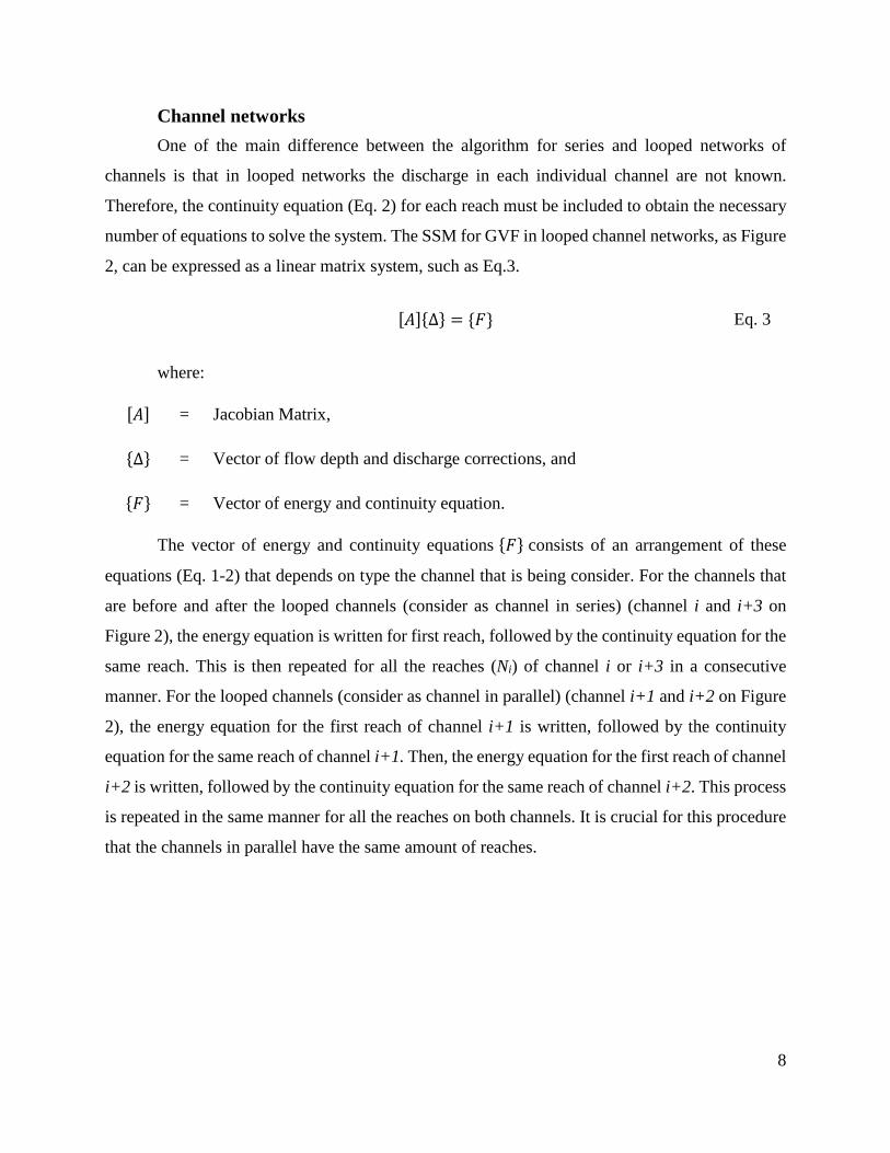
Channel networks

One of the main difference between the algorithm for series and looped networks of

channels is that in looped networks the discharge in each individual channel are not known.

Therefore, the continuity equation (Eq. 2) for each reach must be included to obtain the necessary

number of equations to solve the system. The SSM for GVF in looped channel networks, as Figure

2, can be expressed as a linear matrix system, such as Eq.3.

[𝐴]{∆} = {𝐹} Eq. 3

where:

[𝐴] = Jacobian Matrix,

{∆} = Vector of flow depth and discharge corrections, and

{𝐹} = Vector of energy and continuity equation.

The vector of energy and continuity equations {𝐹} consists of an arrangement of these

equations (Eq. 1-2) that depends on type the channel that is being consider. For the channels that

are before and after the looped channels (consider as channel in series) (channel i and i+3 on

Figure 2), the energy equation is written for first reach, followed by the continuity equation for the

same reach. This is then repeated for all the reaches (Ni) of channel i or i+3 in a consecutive

manner. For the looped channels (consider as channel in parallel) (channel i+1 and i+2 on Figure

2), the energy equation for the first reach of channel i+1 is written, followed by the continuity

equation for the same reach of channel i+1. Then, the energy equation for the first reach of channel

i+2 is written, followed by the continuity equation for the same reach of channel i+2. This process

is repeated in the same manner for all the reaches on both channels. It is crucial for this procedure

that the channels in parallel have the same amount of reaches.

9

Figure 2: Example of a looped channel network.

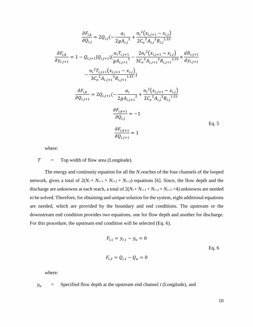
The Jacobian matrix [𝐴] consists of the partial derivatives of the energy and continuity

equations with respect to the flow depth and the discharge. The assembly of this matrix follows

the same pattern as the vector of energy and continuity equation for the channel in series and in

parallel. First, the partial derivative of the energy equation with respect to flow depth is written for

section j of channel i. The second term in the same row will be the derivative of the energy equation

with respect to discharge for the section j of the same channel i. Next, on the same row, the partial

derivative of the energy equation with respect to flow depth is written for section j+1 of channel

i. The last term of this row will be the partial derivative of the energy equation with respect to the

discharge for section j+1 of the same channel i. The following row of the Jacobian matrix will

consist of the partial derivatives of the continuity equation with respect of the discharge, since the

partial derivative with respect of the flow depth is cero. These partial derivatives are shown in Eq.

4 and Eq.5 for the energy and continuity equation, respectively. The vector of flow depth and

discharge corrections {∆} provides the corrections of the flow depth and discharge for all the

sections of all channel. This vector of solutions will be updated at each iteration until the

corrections are smaller than a certain tolerance.

𝜕𝐹𝑖,𝑘

𝜕𝑦𝑖,𝑗= −1 + 𝑄𝑖,𝑗|𝑄𝑖,𝑗|(

𝛼𝑖𝑇𝑖,𝑗

𝑔𝐴𝑖,𝑗3 −

2𝑛𝑖2(𝑥𝑖,𝑗+1 − 𝑥𝑖,𝑗)

3𝐶𝑜2𝐴𝑖,𝑗

2𝑅𝑖,𝑗2.33 ×

𝑑𝑅𝑖,𝑗

𝑑𝑦𝑖,𝑗

−𝑛𝑖

2𝑇𝑖,𝑗(𝑥𝑖,𝑗+1 − 𝑥𝑖,𝑗)


3𝑅𝑖,𝑗1.33 )

Eq. 4

10

𝜕𝐹𝑖,𝑘

𝜕𝑄𝑖,𝑗= 2𝑄𝑖,𝑗(−

𝛼𝑖

2𝑔𝐴𝑖,𝑗2 +

𝑛𝑖2(𝑥𝑖,𝑗+1 − 𝑥𝑖,𝑗)


2𝑅𝑖,𝑗1.33

𝜕𝐹𝑖,𝑘

𝜕𝑦𝑖,𝑗+1= 1 − 𝑄𝑖,𝑗+1|𝑄𝑖,𝑗+1|(

𝛼𝑖𝑇𝑖,𝑗+1

𝑔𝐴𝑖,𝑗+13 −

2𝑛𝑖2(𝑥𝑖,𝑗+1 − 𝑥𝑖,𝑗)

3𝐶𝑜2𝐴𝑖,𝑗+1

2𝑅𝑖,𝑗+12.33 ×

𝑑𝑅𝑖,𝑗+1

𝑑𝑦𝑖,𝑗+1

−𝑛𝑖

2𝑇𝑖,𝑗+1(𝑥𝑖,𝑗+1 − 𝑥𝑖,𝑗)

3𝐶𝑜2𝐴𝑖,𝑗+1

3𝑅𝑖,𝑗+11.33 )

𝜕𝐹𝑖,𝑘

𝜕𝑄𝑖,𝑗+1= 2𝑄𝑖,𝑗+1(−

𝛼𝑖

2𝑔𝐴𝑖,𝑗+12 +

𝑛𝑖2(𝑥𝑖,𝑗+1 − 𝑥𝑖,𝑗)


2𝑅𝑖,𝑗1.33

𝜕𝐹𝑖,𝑘+1

𝜕𝑄𝑖,𝑗= −1

Eq. 5 𝜕𝐹𝑖,𝑘+1

𝜕𝑄𝑖,𝑗+1= 1

where:

𝑇 = Top width of flow area (Longitude).

The energy and continuity equation for all the Ni reaches of the four channels of the looped

network, gives a total of 2(Ni + Ni+1 + Ni+2 + Ni+3) equations [6]. Since, the flow depth and the

discharge are unknowns at each reach, a total of 2(Ni + Ni+1 + Ni+2 + Ni+3 +4) unknowns are needed

to be solved. Therefore, for obtaining and unique solution for the system, eight additional equations

are needed, which are provided by the boundary and end conditions. The upstream or the

downstream end condition provides two equations, one for flow depth and another for discharge.

For this procedure, the upstream end condition will be selected (Eq. 6).

𝐹𝑖,1 = 𝑦𝑖,1 − 𝑦𝑢 = 0

Eq. 6

𝐹𝑖,2 = 𝑄𝑖,1 − 𝑄𝑢 = 0

where:

𝑦𝑢 = Specified flow depth at the upstream end channel i (Longitude), and

11

𝑄𝑢 = Specified discharge at the upstream end channel i (Longitude).

The remaining six equations are provided by boundary conditions at both junction of the

looped network. The upstream junction (jn1) provides three equations, in which one is from the

continuity equation and two are from the energy equation (Eq. 7) (see Figure 3a). In a similar

manner, the downstream junction (jn2) provides the last three equations needed (Eq. 8) (see Figure

3b).

𝐹𝑗𝑛1,1 = 𝑄𝑖,𝑁𝑖+1 − 𝑄𝑖+1,1 − 𝑄𝑖+2,1 = 0

Eq. 7

𝐹𝑗𝑛1,2 = 𝑧𝑖,𝑁𝑖+1 − 𝑧𝑖+1,1 + 𝑦𝑖,𝑁𝑖+1 − 𝑦𝑖+1,1 +

𝑄𝑖,𝑁𝑖+1|𝑄𝑖,𝑁𝑖+1|

2𝑔𝐴𝑖,𝑁𝑖+12

− (𝛼𝑖+1 + ϗ)𝑄𝑖+1,1|𝑄𝑖+1,1|

2𝑔𝐴𝑖+1,12 = 0

𝐹𝑗𝑛1,3 = 𝑧𝑖,𝑁𝑖+1 − 𝑧𝑖+2,1 + 𝑦𝑖,𝑁𝑖+1 − 𝑦𝑖+2,1 +

𝑄𝑖,𝑁𝑖+1|𝑄𝑖,𝑁𝑖+1|

2𝑔𝐴𝑖,𝑁𝑖+12

− (𝛼𝑖+2 + ϗ)𝑄𝑖+2,1|𝑄𝑖+2,1|

2𝑔𝐴𝑖+2,12 = 0

𝐹𝑗𝑛2,1 = 𝑄𝑖+3,1 − 𝑄𝑖+1,𝑁𝑖+1+1 − 𝑄𝑖+2,𝑁𝑖+2+1 = 0

Eq. 8

𝐹𝑗𝑛2,2 = 𝑧𝑖+1,𝑁𝑖+1+1 − 𝑧𝑖+3,1 + 𝑦𝑖+1,𝑁𝑖+1+1 − 𝑦𝑖+3,1

+𝑄𝑖+1,𝑁𝑖+1+1|𝑄𝑖+1,𝑁𝑖+1+1|

2𝑔𝐴𝑖+1,𝑁𝑖+1+12 − (𝛼𝑖+3 + ϗ)

𝑄𝑖+3,1|𝑄𝑖+3,1|

2𝑔𝐴𝑖+3,12 = 0

𝐹𝑗𝑛2,3 = 𝑧𝑖+2,𝑁𝑖+2+1 − 𝑧𝑖+3,1 + 𝑦𝑖+2,𝑁𝑖+2+1 − 𝑦𝑖+3,1

+𝑄𝑖+2,𝑁𝑖+2+1|𝑄𝑖+2,𝑁𝑖+2+1|

2𝑔𝐴𝑖+2,𝑁𝑖+2+12 − (𝛼𝑖+3 + ϗ)

𝑄𝑖+3,1|𝑄𝑖+3,1|

2𝑔𝐴𝑖+3,12 = 0

where:

ϗ = Head-loss coefficient (dimensionless).

12

Figure 3: Definition sketch of a channel junctions in a looped network. a) Upstream junction (jn1); and b) downstream junction

(jn2).

If the equations for a channel network are arbitrarily arranged, then all the nonzero

elements of the Jacobian matrix may not necessarily lie on or near the principal diagonal [13]. This

results in increased storage requirements, increased computer time, and, most probably, reduced

accuracy [13]. For a parallel-channel system with M parallel channels, this arrangement of

equations results in a Jacobian of bandwidth 3M + 1 [13]. In more complex networks, the previous

equations must be included for branching junctions of three channels. Also, for complex channel

networks, there is not a generalized procedure for arranging the equations to produce a Jacobian

matrix of minimum bandwidth, since the system is asymmetric.

Lateral weir design

The lateral weir design depends on the flow depth at the weir. To determine the appropriate

height of the crest (Pw) it’s recommend that as an initial estimate for this value the ratio of the

wetted area to the top width (Pw = Aw/Tw) [14]. Also it’s recommended that the height of the crest

of a suppressed rectangular weir (Figure 4) should be at least equal to three times the maximum

head (hmax) at the weir [15]. Also the sidewalls of the weir must extend at least a distance of 0.3

hmax.

13

Figure 4: Cross section of a suppressed rectangular weir.

The head at the crest of the weir is obtained by subtracting the height of the crest from flow

depth (H=Yw -Pw). For the SM the flow depth at the weir is considered to be the average flow

depth between the section preceding and following section of the weir. This head of water above

the crest is related to the discharge; therefore a higher head of water means an increase of the flow

throughout the weir. To determine the discharge that passes through the weir, the following

equations are used (Eq. 9 to Eq. 11). This flow can be a maximum of 25% of the original discharge

that flows through the main channel [16].

𝑄𝑤 = 𝐶𝑒𝐿𝑤𝐻3/2 Eq. 9

𝐶𝑒 =2

3𝐶𝑑√2𝑔 Eq. 10

𝐶𝑑 = 0.485 (2 − 𝐹𝑟2

2 + 3𝐹𝑟2)0.5 Eq. 11

where:

𝐿𝑤 = Length of the weir (Longitude),

𝐻 = Head above the weir (Longitude),

𝐶𝑒 = Effective discharge coefficient (dimensionless),

𝐶𝑑 = Discharge coefficient (dimensionless), and

𝐹𝑟 = Froude number (dimensionless).

14

When a lateral weir is incorporated to the series of channel, in the SSM, produces a division

of the existing channel into two new channels, with the same geometric properties of the existing

channel, joined by the lateral weir. This new junction can be represented as series junction criteria,

since the flow through the weir will reduce the flow through the main channel and will modify the

energy equation vector and the Jacobian matrix. The main modification is the addition of the weir

flow to the continuity equation (Eq. 2), since a value is now available and there will be a reduction

on the flow at the main channel. The design criteria for the lateral weir consists of determining the

length of the weir necessary to produce a specific discharge throughout the weir that will irrigate

a specific parcel. Therefore, the weir flow desired will be given to the algorithm, as a percent of

the discharge upstream of the weir location. Also, an initial estimate of the height of the crest is

given to the algorithm. It is important to verify with the solution if the height of the crest meets the

minimum criteria proposed by the U.S. Bureau of Reclamation. With the flow depth calculated,

the coefficient of discharge and effective coefficient of discharge is obtained, to finally determine

the length of the weir from Eq. 9.

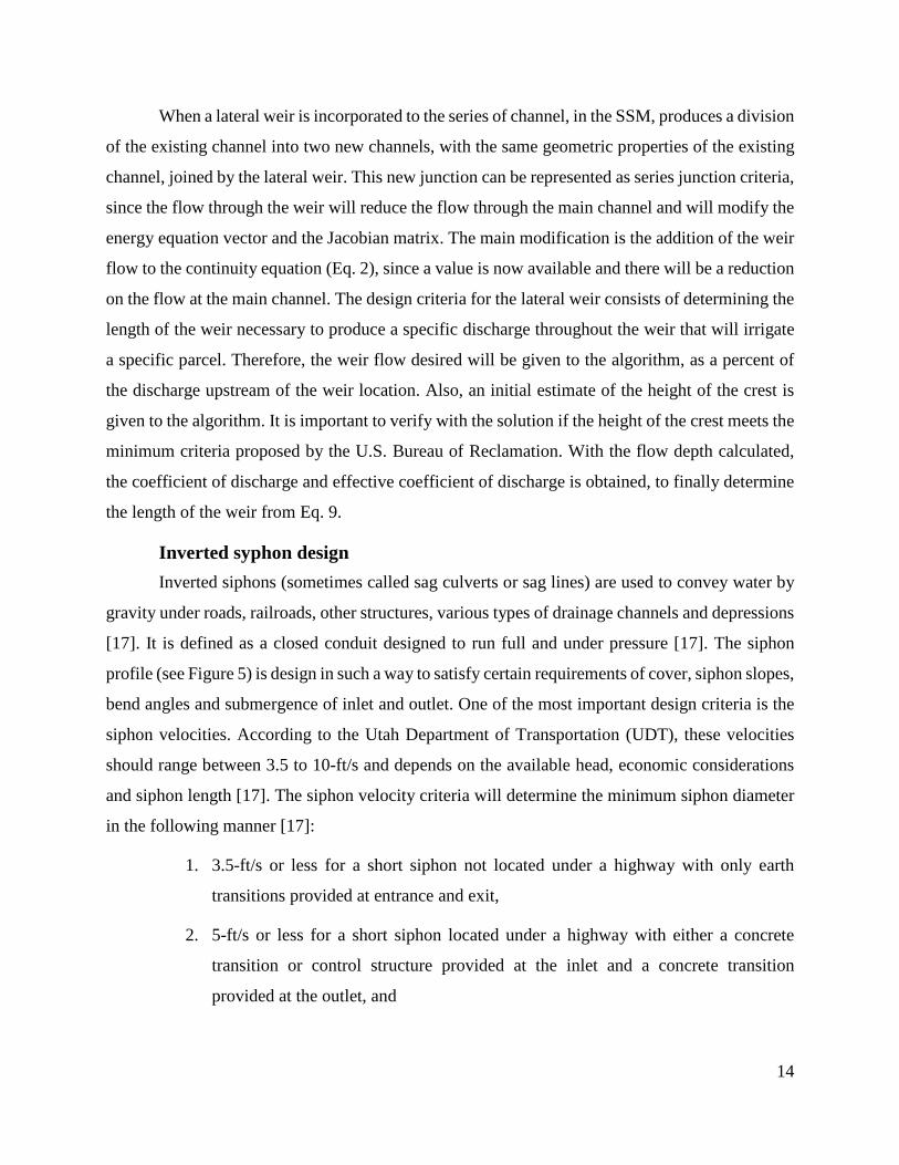
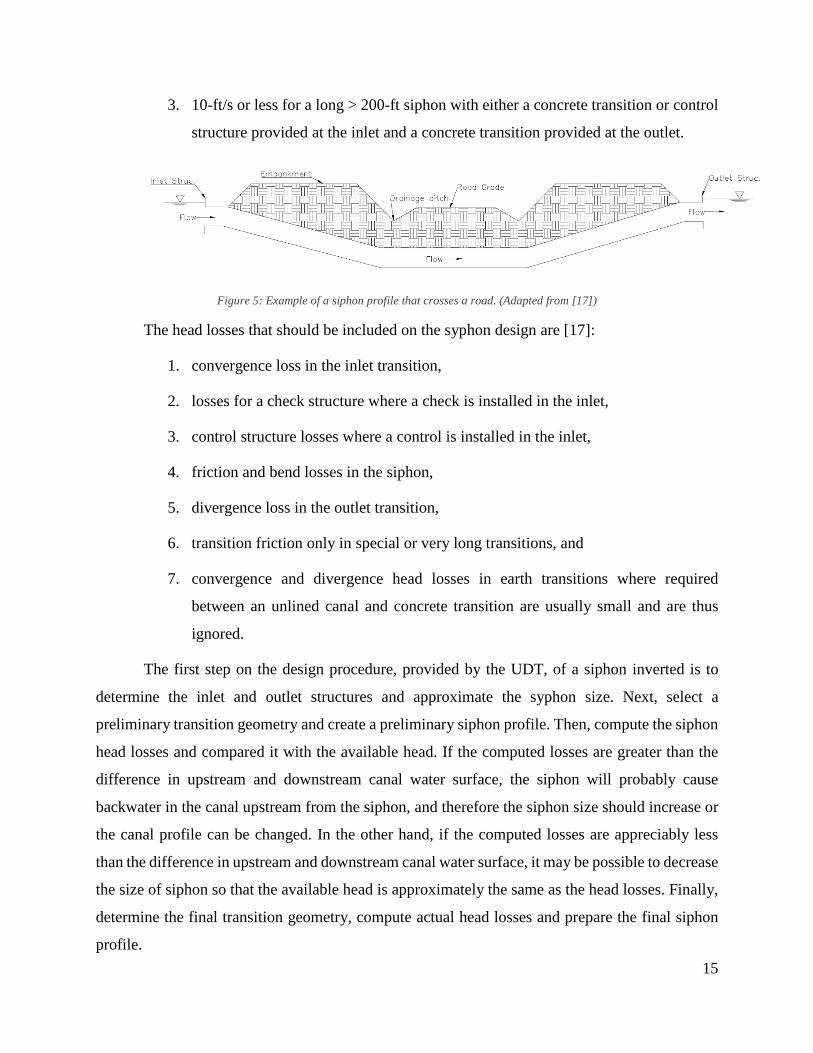
Inverted syphon design

Inverted siphons (sometimes called sag culverts or sag lines) are used to convey water by

gravity under roads, railroads, other structures, various types of drainage channels and depressions

[17]. It is defined as a closed conduit designed to run full and under pressure [17]. The siphon

profile (see Figure 5) is design in such a way to satisfy certain requirements of cover, siphon slopes,

bend angles and submergence of inlet and outlet. One of the most important design criteria is the

siphon velocities. According to the Utah Department of Transportation (UDT), these velocities

should range between 3.5 to 10-ft/s and depends on the available head, economic considerations

and siphon length [17]. The siphon velocity criteria will determine the minimum siphon diameter

in the following manner [17]:

1. 3.5-ft/s or less for a short siphon not located under a highway with only earth

transitions provided at entrance and exit,

2. 5-ft/s or less for a short siphon located under a highway with either a concrete

transition or control structure provided at the inlet and a concrete transition

provided at the outlet, and

15

3. 10-ft/s or less for a long > 200-ft siphon with either a concrete transition or control

structure provided at the inlet and a concrete transition provided at the outlet.

Figure 5: Example of a siphon profile that crosses a road. (Adapted from [17])

The head losses that should be included on the syphon design are [17]:

1. convergence loss in the inlet transition,

2. losses for a check structure where a check is installed in the inlet,

3. control structure losses where a control is installed in the inlet,

4. friction and bend losses in the siphon,

5. divergence loss in the outlet transition,

6. transition friction only in special or very long transitions, and

7. convergence and divergence head losses in earth transitions where required

between an unlined canal and concrete transition are usually small and are thus

ignored.

The first step on the design procedure, provided by the UDT, of a siphon inverted is to

determine the inlet and outlet structures and approximate the syphon size. Next, select a

preliminary transition geometry and create a preliminary siphon profile. Then, compute the siphon

head losses and compared it with the available head. If the computed losses are greater than the

difference in upstream and downstream canal water surface, the siphon will probably cause

backwater in the canal upstream from the siphon, and therefore the siphon size should increase or

the canal profile can be changed. In the other hand, if the computed losses are appreciably less

than the difference in upstream and downstream canal water surface, it may be possible to decrease

the size of siphon so that the available head is approximately the same as the head losses. Finally,

determine the final transition geometry, compute actual head losses and prepare the final siphon

profile.

16

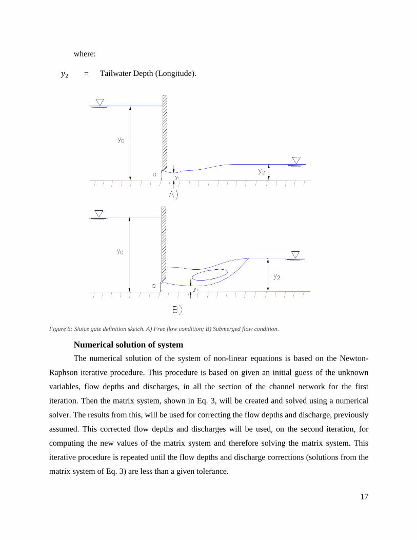
Sluice gates design

A sluice gate is an opening in a hydraulic structure used for controlling the discharge [18].

Figure 6 shows the definition sketch for free flow and submerged flow sluice gate. Downstream

free flow occurs at a (relatively) large ratio of upstream depth to the gate-opening height [18].

However, submerged flow at the downstream would occur for low values of this ratio [18]. The

conventional sluice gate discharge equation is written in the following form (Eq.12):

𝑄𝑠 = 𝐶′𝑑𝑎𝑏√2𝑔𝑦0 Eq. 12

where:

𝑄𝑠 = Sluice gate discharge (Volume/time),

𝐶′𝑑 = Sluice gate discharge coefficient (depends on the flow condition)

(dimensionless),

𝑎 = Sluice gate opening (Longitude),

𝑏 = Sluice gate length (Longitude), and

𝑦0 = Upstream water depth (Longitude).

The free flow condition can be defined as Eq. 13 and the submerged flow conditions can

be defined as Eq. 14 [18]. Depending on the flow conditions the sluice gate discharge coefficient

can be defined as Eq. 15 or Eq. 16 for free flow and submerged flow conditions, respectively.

𝑦0 ≥ 0.81𝑦2(𝑦2

𝑎)0.72 Eq. 13

𝑦2 ≤ 𝑦0 ≤ 0.81𝑦2(𝑦2

𝑎)0.72 Eq. 14

𝐶′𝑑 = 0.611(𝑦0 − 𝑎

𝑦0 + 15𝑎)0.072 Eq. 15

𝐶′𝑑 = 0.611 (

𝑦0 − 𝑎

𝑦0 + 15𝑎)

0.072

(𝑦0 − 𝑦2)0.7{0.32 [0.81𝑦2 (𝑦2

𝑎)

0.72

− 𝑦0]0.7

+ (𝑦0 − 𝑦2)0.7}−1

Eq. 16

17

where:

𝑦2 = Tailwater Depth (Longitude).

Figure 6: Sluice gate definition sketch. A) Free flow condition; B) Submerged flow condition.

Numerical solution of system

The numerical solution of the system of non-linear equations is based on the Newton-

Raphson iterative procedure. This procedure is based on given an initial guess of the unknown

variables, flow depths and discharges, in all the section of the channel network for the first

iteration. Then the matrix system, shown in Eq. 3, will be created and solved using a numerical

solver. The results from this, will be used for correcting the flow depths and discharge, previously

assumed. This corrected flow depths and discharges will be used, on the second iteration, for

computing the new values of the matrix system and therefore solving the matrix system. This

iterative procedure is repeated until the flow depths and discharge corrections (solutions from the

matrix system of Eq. 3) are less than a given tolerance.

18

The numerical solver selected was the Bi-conjugated Gradient Stabilizer with

Preconditioner method (BiCGSTAB). BiCGSTAB is a variation of the Conjugate Gradient

Squared method, which is based on squaring the residual polynomial and may lead to substantial

build-up of rounding errors [19]. The BiCGSTAB is design to solve non-symmetric positive

definite system that are large and sparse linear system, such as our system. Since our matrix system

is ill-conditioned and is non-diagonally dominant, the preconditioner used with BiCGSTAB was

the incomplete LU factorization (iLU) with threshold and pivoting. iLU produces a unit lower

triangular matrix, and an upper triangular matrix, in which the ceros on the original matrix are

preserve on the produced matrices; preserving the sparsity of the system. The pivoting of the iLU

helps to avoid that an element close to the main diagonal is cero, which can produce numerical

destabilization.

Preliminary results

Some preliminary results have been already developed from the proposed algorithm. The

algorithm is capable of solving for the flow depths and discharges of looped channel networks

with analysis and/or design of lateral weir. Figure 7 shows a sketch of the proposed case study of

a looped channel network that contains five lateral weirs and 11 trapezoidal channels that have

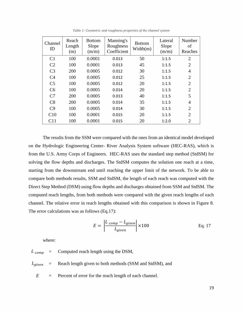
different geometric properties and amount of reaches. Table 1 shows details of the geometric and

roughness properties for the channel system used as a case study.

Figure 7: Case study of a looped channel network with lateral weirs.

19

Table 1: Geometric and roughness properties of the channel system

Channel

ID

Reach

Length

(m)

Bottom

Slope

(m/m)

Manning's

Roughness

Coefficient

Bottom

Width(m)

Lateral

Slope

(m/m)

Number

of

Reaches

C1 100 0.0001 0.013 50 1:1.5 2

C2 100 0.0001 0.013 45 1:1.5 2

C3 200 0.0005 0.012 30 1:1.5 4

C4 100 0.0005 0.012 25 1:1.5 2

C5 100 0.0005 0.012 20 1:1.5 2

C6 100 0.0005 0.014 20 1:1.5 2

C7 200 0.0005 0.013 40 1:1.5 5

C8 200 0.0005 0.014 35 1:1.5 4

C9 100 0.0005 0.014 30 1:1.5 2

C10 100 0.0001 0.015 20 1:1.5 2

C11 100 0.0001 0.015 20 1:2.0 2

The results from the SSM were compared with the ones from an identical model developed

on the Hydrologic Engineering Center- River Analysis System software (HEC-RAS), which is

from the U.S. Army Corps of Engineers. HEC-RAS uses the standard step method (StdSM) for

solving the flow depths and discharges. The StdSM computes the solution one reach at a time,

starting from the downstream end until reaching the upper limit of the network. To be able to

compare both methods results, SSM and StdSM, the length of each reach was computed with the

Direct Step Method (DSM) using flow depths and discharges obtained from SSM and StdSM. The

computed reach lengths, from both methods were compared with the given reach lengths of each

channel. The relative error in reach lengths obtained with this comparison is shown in Figure 8.

The error calculations was as follows (Eq.17):

𝐸 = |𝐿 𝑐𝑜𝑚𝑝 − 𝐿𝑔𝑖𝑣𝑒𝑛

𝐿𝑔𝑖𝑣𝑒𝑛| ×100 Eq. 17

where:

𝐿 𝑐𝑜𝑚𝑝 = Computed reach length using the DSM,

𝐿𝑔𝑖𝑣𝑒𝑛 = Reach length given to both methods (SSM and StdSM), and

𝐸 = Percent of error for the reach length of each channel.

20

The SSM have significant lower percent of error for reach length than HEC-RAS- StdSM,

giving confidence that the proposed algorithm is accurate in calculating the flow depth and

discharges in looped channel networks with lateral weirs.

Figure 8: Percent of error for reach length of both method results for the case study of the looped channel network.

References

[1] Irrigation Museum (2015). Irrigation Timeline [Online]. Available:

http://www.irrigationmuseum.org/exhibit2.aspx [March 22, 2016].

[2] A.M. Michael, “Utilization of Water Resources and Irrigation Development” in Irrigation: Theory and

Principles, 2nd ed. Jangpura, India: Vikas Publishing House, 2008, ch. 1, pp. 1-6.

[3] United Nations Sustainable Development, “Agenda 21”, in United Nations Conference on Environmental and

Development, Rio de Janeiro, Brazil, 1992, pp. 18.1-18.90.

[4] Departamento de Recursos Naturales de Puerto Rico (2008). Plan Integral de Aguas de Puerto Rico [Online].

Available: http://www.recursosaguapuertorico.com/Cuencas-Principales-en-PR.html [March 22, 2016].

[5] M. H. Chaudhry and A. M. Schulte, “Computation of steady-state, gradually varied flow in parallel channels”, in

Canadian Journal of Civil Engineering, vol. 13, pp. 39-45, 1986.

[6] M. H. Chaudhry and A. M. Schulte, “Gradually-varied flows in open-channel network”, in Journal of Hydraulic

Research, vol. 25, pp. 357-371, 1987.

[7] B. J. Naidu et al., “GVF Computation in Tree-type Channel Networks”, in Journal of Hydraulic Engineering, vol.

131, pp. 457-465, Aug. 1997.

[8] H. P. Reddy and S. M. Bhallamudi, “Gradually Varied Flow Computations in Cyclic Looped Channel Networks”,

in Journal of Irrigation and Drainage Engineering, vol. 130, pp. 424–431, Oct. 2004.

0.011%

0.009%

0.001%

0.001%

0.001%

0.001%

0.001%

0.001%

0.001%

0.062%

0.030%

20.773%

0.4%

0.4%

0.6%

19.362%

0.4%

0.7%

0.7%

28.51%

16.89%

0% 5% 10% 15% 20% 25% 30%

1

2

3

4

5

6

7

8

9

10

11

Channel N

um

ber

Percent of Error for Reach Length StdSM SSM

21

[9] D. J. Sen and N. K. Garg, “Efficient Algorithm for Gradually Varied Flows in Channel Networks”, in Journal of

Irrigation and Drainage Engineering, vol. 128, pp. 351-357, Nov. 2002.

[10] A. Islam et al., “Comparison of Gradually Varied Flow Computation Algorithms for Open-Channel Network”,

in Journal of Irrigation and Drainage Engineering, vol. 123, pp. 457-465, Sept. 2005.

[11] A. Islam et al., “Development and Application of Hydraulic Simulation Model for Irrigation Canal Networks”,

in Journal of Irrigation and Drainage Engineering, vol. 134, pp. 49-59, Feb. 2008.

[12] D. Zhu et al., “Simple, Robust, and Efficient Algorithm for Gradually Varied Subcritical Flow Simulation in

General Channel Networks”, in Journal of Hydraulic Engineering, vol. 137, pp. 766-774, July 2011.

[13] H. M. Chaudhry, “Computation of Gradually Varied Flow” in Open-Channel Flow, 2nd ed. New York, NY:

Springer Science, 2008, ch.6, pp.150-197.

[14] R. W. P. May et al., “Design Considerations” in Hydraulic Design of Side Weirs, 1st ed. Reston, VA: Thomas

Telford Publishing, 2003, ch. 3, pp. 15-23

[15] U. S. Department of the Interior: Bureau of Reclamation, “Weirs” in Water Measurement Manual, 3rd ed.

Washington, DC: U.S. Government Printing Office, 2001, ch. 7, pp. 7.1-7.30

[16] V. M. Vargas, “Hydraulic Design of an Overland Flow Distribution System Using Lateral Weirs”, M.S. thesis,

Dept. Civil Engineering and Surveying, Univ. of Puerto Rico, Mayagüez, PR, 2014.

[17] Utah Department of Transportation (2004). Manual of Instruction: Roadway Drainage [Online]. Available:

https://www.udot.utah.gov/main/f?p=100:pg:0:::1:T,V:826, [July 10, 2016].

[18] P.K. Swamee, “Sluice-Gate Discharge Equations”, in Journal of Irrigation and Drainage Engineering, vol. 118,

pp. 56-60, Feb. 1992.

[19] Y. Saad, “Krylov Subspace Methods part II”, in Iterative Methods for Sparse Linear System, 2nd ed.

Philadelphia, PA: SIAM, 2003, ch. 7, pp. 229-258.

computation of gradually varied flow in channel networks...

Documents