Preprint, February 1, 2004 1

Computation of the Fractional Fourier Transform

Adhemar Bultheel and Hector E. Martınez Sulbaran 1

Dept. of Computer Science, Celestijnenlaan 200A, B-3001 Leuven

Abstract

In this note we make a critical comparison of some matlab programs for the digital computation of thefractional Fourier transform that are freely available and we describe our own implementation that filtersthe best out of the existing ones. Two types of transforms are considered: First the fast approximatefractional Fourier transform algorithm for which two algorithms are available. The method is describedin H.M. Ozaktas, M.A. Kutay, and G. Bozdagi. Digital computation of the fractional Fourier transform.

IEEE Trans. Signal Process., 44:2141–2150, 1996. There are two implementations: one is written byA.M. Kutay the other is part of package written by J. O’Neill. Secondly the discrete fractional Fouriertransform algorithm described in the master thesis C. Candan. The discrete fractional Fourier transform,Bilkent Univ., 1998 and an algorithm described by S.C. Pei, M.H. Yeh, and C.C Tseng: Digital fractional

Fourier transform based on orthogonal projections IEEE Trans. Signal Process., 47:1335–1348, 1999.

Key words: Fractional Fourier transform

1 Introduction

The idea of fractional powers of the Fourier transform operator appears in the mathematicalliterature as early as 1929 [23,9,11]. Later on it was used in quantum mechanics [14,13] and signalprocessing [1], but it was mainly the optical interpretation and the applications in optics that gavea burst of publications since the 1990’s that culminated in the book of Ozaktas et al [17].

The reason for its success in optical applications can be explained as follows. Consider a systemwhich consists of a point light source on the left. The light illuminates an object after traversing aset of optical components like e.g. thin lenses. It is then well known that at certain points to theright of the object one may observe images that are the Fourier transform of the object image.Somewhat further it is the inverted object image, still further it becomes the inverted Fouriertransform and still further it is the upright image etc. These images are obtained by the Fourieroperator applied to the object image, its second power (the inverted image), the 3rd power (the

1 The work of the first author is partially supported by the Fund for Scientific Research (FWO), pro-jects “CORFU: Constructive study of orthogonal functions”, grant #G.0184.02 and, “SMA: Structuredmatrices and their applications”, grant G#0078.01, “ANCILA: Asymptotic analysis of the convergencebehavior of iterative methods in numerical linear algebra”, grant #G.0176.02, the K.U.Leuven researchproject “SLAP: Structured linear algebra package”, grant OT-00-16, the Belgian Programme on Interuni-versity Poles of Attraction, initiated by the Belgian State, Prime Minister’s Office for Science, Technologyand Culture. The scientific responsibility rests with the author.

1

inverted Fourier image) and the 4th power (the original image), etc. The images in between arethe result of intermediate (fractional) powers of the Fourier operator applied to the image object.

Like for the Fourier transform, there exists a discrete version of the fractional Fourier transform. Itis based on an eigenvalue decomposition of the discrete Fourier transform matrix. If F = EΛE−1 isthis decomposition then F a = EΛaE−1 is the corresponding discrete fractional Fourier transform.

As far as we know, there are not many public domain software routines available for the compu-tation of the (discrete) fractional Fourier transform. We are aware of only two routines. There isthe one that can be found on the web site [12] of the book [17] previously described in Ozaktas[16] and another one which is part of a package compiled by O’Neill. In this note we shall analysethe advantages and disadvantages of the two algorithms and propose some improvements.

The text is organized as follows. In Section 2 we briefly recall the mathematical background ofthe (discrete) fractional Fourier transform. Section 3 describes the algorithm of Candan and theimplementation aspects are discussed in the subsequent section 4. Some modifications are proposedin section 5. The theory of the discrete transform is given on section 6 and the practical aspects arefound in section 7. The performance in approximating the Gauss-Hermite functions are illustratedin section 8 and its approximation of the fast approximate transform in section 10. In section 9alternative definitions of the discrete fractional Fourier transform are briefly discussed. Finally insection 11, an illustration of the algorithms on de two dimensional example is given.

2 Mathematical Background

In this section we introduce the definition of the continuous fractional Fourier transform (FrFT)and the discrete fractional Fourier transform.

Definition 1 (Continuous Fractional Fourier Transform) The fractional Fourier transformFa of order a ∈ R is a linear integral operator that maps a given function (signal) f(x), x ∈ R

onto fa(ξ), ξ ∈ R by

fa(ξ) = Fa(ξ) =

+∞∫

−∞

Ka(ξ, x)f(x)dx

where the kernel is defined as follows. Set α = aπ/2 then

Ka(ξ, x) = Cα exp

{

−iπ(

2xξ

sinα− (x2 + ξ2) cotα

)}

,

with

Cα =√

1 − i cotα =exp{−i[πsgn(sinα)/4 − α/2]}

√

| sinα|.

For k ∈ 2Z, limiting values are taken.

2

Note that for a ∈ 4Z, the FrFT becomes the identity f4k(ξ) = f(ξ), hence the kernel is in thatcase

K4k(ξ, x) = δ(ξ − x), k ∈ Z

and for a ∈ 2 + 4Z, this is the parity operator f2+4k(ξ) = f(−ξ), corresponding to the kernel

K2+4k(ξ, x) = δ(ξ + x), k ∈ Z,

while for a ∈ 1+4Z, Fa = F1 is just the Fourier operator F , and for a ∈ 3+4Z, F a = F3 = F2F ,in other words, if f1(ξ) = Ff(x) is the Fourier transform, then f3(ξ) = f1(−ξ).

This should make clear that Fa can be interpreted as the ath power of the Fourier transform whichmay be interpreted modulo 4. So, we have for example the well known properties F aF b = Fa+b

and F−aFa = I is the identity.

In the theory of the fractional Fourier transform, a special role is played by a chirp function.

Definition 2 (Chirp function) A chirp is a function that sweeps a certain frequency interval[ω0, ω1] in a certain time interval [t0, t1]. If the sweep rate is linear, it has the form exp{iπ(χx+γ)x}with χ the sweep rate.

Note that Fa(δ(x− γ)) = Ka(ξ, γ) is a chirp with sweep rate cotα.

Note also that

x2 cotα− 2xξ cscα + ξ2 cotα = x2(cotα− cscα) + (x− ξ)2 cscα + ξ2(cotα− cscα).

Thus the fractional Fourier transform can be seen as applying a chirp convolution with sweep ratecscα in between two chirp multiplications with sweep rate cotα.

If the signal f consists of only a finite number of discrete samples, we have to define a correspondingdiscrete fractional Fourier transform. We shall introduce that via the classical discrete Fouriertransform.

Definition 3 (Discrete Fourier Transform) The discrete Fourier transform of a vector f =[f(0), . . . , f(N − 1)]T is defined as the vector f1 = Ff where the N×N DFT matrix F has entriesthat are the N th roots of unity: F (k, n) = W kn/

√N with W = e−i2π/N . Hence

f1(k) =N−1∑

n=0

F (k, n)f(n) =1√N

N−1∑

n=0

f(n)e−i 2πk

N , k = 0, . . . , N − 1.

The DFT matrix F satisfies F 4 = I with I the identity matrix. It has the eigenvalues {1,−i,−1, i} ={eikπ/2 : k = 0, . . . , N − 1}. It has also N independent orthonormal eigenvectors that can be ar-ranged as the columns of a matrix E, so that its eigenvalue decomposition is F = EΛET . Thedefinition of the discrete fractional Fourier transform is then easily given as a multiplication witha (fractional) power of the Fourier matrix. Note however that the choice of the set of eigenvectors

3

for the matrix F is not unique, even if we suppose them to be orthonormal. There are only foueigenvalues and the choice of the (orthonormal) basisvectors within each eigenspace is not unique.There are some arguments, that require a particular choice of these eigenvectors which imposecertain symmetry conditions as we shall see later, and this will fix the eigenvectors uniquely.

Definition 4 (Discrete Fractional Fourier Transform) A discrete fractional Fourier trans-form of a vector f = [f(0), . . . , f(N − 1)]T is defined as the vector fa = F af , i.e., the vector withcomponents

fa(k) = F af =N−1∑

n=0

F a(k, n)f(n), k = 0, . . . , N − 1,

where F a = EΛaET , with F = EΛET an eigenvalue decomposition of the DFT matrix.

Besides the ambiguity in the choice of the eigenvectors that we mentioned before, also the choiceof the branch in the powers Λa for a real introduces another ambiguity which can be given aneasy solution because the eigenvalus in the discrete case are {e−nπ/2} with n = 0, 1, 2, . . ., whichis a cyclic repetition of {−i,−1, i, 1}, and then the powers can be defined as e−ianπ/2 for a real.

The discrete fractional Fourier transform can be used as an approximation of the continuousfractional Fourier transform when N is large as will be explained in section 8. But there is a moredirect and faster way to compute an approximation of the continuous fractional Fourier transform,as will be explained now.

3 Fast computation of the continuous fractional Fourier transform algorithms

The algorithms considered here are algorithms that approximate the continuous fractional Fouriertransform in the sense that they map samples of the signal to samples of the samples of thecontinuous fractional Fourier transform. Because it uses FFT techniques with complexity N logN ,it is a fast algorithm. However, it is not really the fractional analog of the Fast Fourier Transform(FFT) which is a particular fast implementation of the Discrete Fourier Transform (DFT). Andalthough it implements just the FFT when the power a = 1 and the inverse FFT when a = 3,and although some authors have coined it fast fractional Fourier transforms, we deliberately avoidto use this term, and call it fast approximate fractional Fourier transform (FAFrFT). For themoment, the fast implementation of the discrete fractional Fourier transform which would be thegenuine fast fractional Fourier transform (FFrFT), is yet unknown.

The continuous integral transform is approximated by a quadrature formula using samples of theoriginal function and computing only samples of the transformed function. We are aware of twomatlab implementations of the fast approximate fractional Fourier transform.

First there is the matlab routine fracF, implementing the algorithm described in [16] (see also[17, Section 6.7]). It can we found on the web page [12].

The second one is another matlab code fracft, which is part of a software package developed byJ. O’Neill, now available at the mathworks website [15]. It also refers to the same paper but hassome differences in implementation.

For completeness, we recall briefly the idea of the algorithm. As we mentioned before, the definition

4

is rewritten in the form of a convolution in between two chirp multiplications. Using cotα−cscα =− tan(α/2), we have

fa(ξ) = Cαe−iπ tan(α/2)ξ2

+∞∫

−∞

eiπ csc α (ξ−x)2 [e−iπ tan(α/2) x2

f(x)]dx.

A first approximation consists in assuming that the functions can be confined to the interval[−∆/2,∆/2] in all time-frequency directions. This means that the Wigner distribution is essentiallyconfined to a circle with radius ∆/2 around the origin of the time-frequency plane. As explained inthe appendix A of [16]. The Wigner distribution of a chirp multiplication and of a chirp convolutionfor an f under consideration, will be compact and contained in a circle with radius ∆. That istwice the original support. Therefore the integral can be restricted to the interval [−∆,∆]. Also,if we want to recover the result from discrete samples, then we should have samples at intervals1/2∆. Thus, assuming we have N = ∆2 samples of the original f , then we need at least 2Nsamples of the convolution. So the integral sampled at ξk = k/2∆ can be approximated as

fa(ξk) ≈Cα

2∆e−iπξ2

ktan(α/2)

N−1∑

l=−N

g(k − l)h(l) (1)

with xk = k/2∆ and

g(k) = eiπx2

kcsc α, h(k) = e−iπx2

ktan(α/2)f(xk).

This gives a discrete approximation of the continuous transform. The convolution has O(N logN)complexity when using FFT. Therefore it is called a fast approximate fractional Fourier transform.

4 Implementation details

A straightforward implementation of this algorithm does not lead to satisfactory results. Let usinvestigate the different steps in detail.

4.1 The length of the signal

Note that in the previous derivation it is assumed that the length of the signal is 2N , henceeven. The routine fracF is a direct implementation of these formulas and therefore requires thesignal length to be even. However, this causes the summations in the previous formulas not tobe completely symmetric. The lower bound is indeed −N while the upper bound is N − 1. Topreserve symmetry, it seems much more convenient to assume that the signal length is odd. Inthat case, the summations can be made completely symmetric. That is why in the routine fracft,the signal length is assumed to be odd. In fact the formulas were chosen symmetric in [16] andnonsymmetric in [17, Section 6.7].

5

4.2 The FFT as a special case

Classically the FFT is defined as a transformation of a vector [f(0), . . . , f(N − 1)], and it isimplemented in this way in the matlab routine fft. If we compare this with the definition ofthe fast approximate fractional Fourier transform given above, where the signal is assumed to be[f(−N), . . . , f(N − 1)], then it is obvious that the routine fft will not give the same result as analgorithm implementing (1) with a = 1. They will only match when the signal and its FFT arecyclically shifted over (approximately) half the signal length. For example, if the length N of thesignal is even, then the FFT should be computed as SFSf , where S is the cyclic shift over N/2samples. For any N , we have implemented this as

shft = rem((0:N-1)+fix(N/2),N)+1;

SFSf(shft) = fft(f(shft))/sqrt(N);

The square root is needed for the normalization that we introduced in our definition. A similarobservation holds for the inverse FFT: fft is replaced by ifft and the division by the square rootis replaced by a multiplication by the square root.

In fracF this cyclic shift is avoided by computing the FFT and its inverse using the generalroutine, so that for F±1 is computed in exactly the same way as for general F a.

In fracft, a cyclic shift is implemented which essentially corresponds to what we described above.Since the signal length is assumed to be odd, this operation introduces some asymmetry whichmay result in a shift of one sample when comparing the results of the two algorithms.

4.3 The reduction of the interval for a

Because we can compute the fractional Fourier transform for a value of a modulo 4, and by usingfurther additivity properties of a, it can be reduced to an interval of length 2, with an additional(inverse) FFT.

The code fracF assumes that −2 ≤ a ≤ 2 and reduces this interval further by the following tests

• if 0 < a < 0.5 then Fa = FFa−1

• if −0.5 < a < 0 then Fa = F−1Fa+1

• if 1.5 < a < 2 then Fa = FFa−1

• if −2 < a < −1.5 then Fa = F−1Fa+1.

In this way we are left with values of a satisfying 0.5 < |a| < 1.5.

In the code fracft, a can take any value and it is reduced to the interval 0.5 ≤ a ≤ 1.5 bythe following tests. First a is replaced by the residual of a/4 reducing a to the interval [0, 4).This interval is reduced to [0, 2] by using F a = F2Fa−2 if a > 2. Note that F 2 just reverses theinput signal and is thus a trivial operation. Next by the following tests, it is further reduced to0.5 ≤ a ≤ 1.5.

• if a > 1.5 then Fa = FFa−1

6

• if a < 0.5 then Fa = F−1Fa+1.

Both approaches are equally good, although we think the second one is a bit simpler. Besides thisreduction, the special cases of integer a, i.e. a ∈ {0, 1, 2, 3} can be handled directly, and do notneed the complicated computation.

In both cases one has to take care that if we compute F af for a ranging over the interval [0, 4],then, depending on further implementation details, it may happen that for example the transitionfrom a just smaller than 1.5 and a just larger than 1.5 is not very smooth. The reason being thatjust before a = 1.5, the transformation F a is computed for the original signal, while just aftera = 1.5, the transformation Fa−1 is computed for the FFT of the signal. And since we are dealingwith a finite number of samples, and not with a continuous signal, all the computations (includingthe FFT) are only approximations of the actual transformation one wants to perform. Similarproblems may arise for the transition from a value of a close to an integer to the integer valueitself. That is probably the reason why in the code fracF, the FFT and inverse FFT operationsare performed via the general routine for the FrFT. Thus actually using the formula (1) withα = ±π/2:

f±1(ξk) ≈C±π/2

2∆e−iπx2

k

N−1∑

l=−N

e±iπx2

k−le−iπx2

l f(xl).

For a value of a = 2.0001, and f = sin(x) sampled in the interval [0, π], the routine fracF givesan irregular shaped answer, while fracft produces a smooth answer that is approximately equalto the reversed signal F 2f . The reason is that F 2.0001f is computed as F1.0001[Ff ] and the FFTthat is involved here is computed by the general routine instead of calling the built in routine fft.

4.4 The core of the routine

The heart of the routine consists of three steps:

• multiplication of f with a chirp function• this result is convolved with a chirp (multiply their Fourier transforms)• multiply with a chirp.

Thus if Ec represents the chirp function eicx2

, then the approximation (1) can be written as

Faf ≈ Cα

2∆Ec F−1{F [Edf ] · F [Ecf ]} (2)

where c = cotα − cscα = − tan(α/2) and d = cscα. However, a direct implementation of thistechnique does not lead to accurate results. As explained in the appendix A of [16], the bandwidthafter chirp multiplication can be doubled, so that we need to double the number of samples toavoid aliassing. A similar argument holds for the convolution. Therefore both routines fracF andfracft replace the signal f of length N by a longer signal obtained by interpolation.

In fracF if is assumed that f has an even length and using sinc interpolation, its length is doubled.By padding it before and after by N zeros, it has length 4N .

7

In fracft, it is assumed that f has an odd length and again using sinc interpolation, insertingp − 1 values in between two successive sample values, it gets length pN − p + 1. The author haschosen p = 3. The result is padded with N − 1 zeros before and after which results in a signal oflength 5N − 4.

4.5 Subsampling of the result

Since the result has to be a signal of the same length as the original signal, the long signal has tobe subsampled. The reason for expanding the signal and padding it with zeros was mainly becausethe convolution of g and h in the formula (1) will not be contaminated by boundary effects in themiddle of the convolution signal.

In fracF, the signals to be convolved are padded with zeros to a length that is the nearest powerof 2, the convolution is then computed as the inverse FFT of the product of the FFTs of the twosignals. As a result, the middle coefficients are selected.

In fracft however, the computation is more subtle. The main operation is a call of the matlabroutine lconv, which does the same as described above, but before the convolution is computed,the signal is once more interpolated. The number of interpolation points inserted in between twovalues depends on the value of d in the formula (2), thus on the value of a. The subroutine iswritten with more general applications in mind because in our situation there is no interpolationnecessary, because for all values of a ∈ [0.5, 1.5] the formula always finds that the number ofinterpolation points needed is 0.

4.6 The interpolation algorithm

The interpolation can be performed in several ways. Sinc interpolation is popular in these applic-ations. The sinc interpolant of f for the interpolation points {xk = k/2∆ : k = −N, . . . , N − 1},(here ∆ =

√N) is given by

y(x) =N−1∑

k=−N

f(xk)sinc(2∆(x− xk)).

Thus it can be computed by either a convolution of the signal with a sinc function (as in fracft)or it can be applied explicitly using an FFT and an inverse FFT (as in fracF). In both cases itrequires O(M logM) operations if the signal has length M .

If M is large, it might seem to be faster to use Lagrange interpolation. Indeed, assuming we wantto insert one interpolation point in between two successive values, we can use an interpolatingpolynomial in {f(xk−1), f(xk), f(xk+1), f(xk+2)} and evaluate it in x1/2, to get an interpolatingvalue in f(xk+1/2). For the boundaries, i.e., for k = 1 or k = N − 2, we evaluate it in xk−1/2,respectively in xk+3/2 to obtain values for f(x3/2) and f(xN−1/2). This means that we obtainf(xk+1/2) as

[−f(xk−1) + 9f(xk) + 9f(xk+1) − f(xk+2)]/16 if k = 2, . . . , N − 3

8

while

f(x3/2) = [5f(x1) + 15f(x2) − 5f(x3) + f(x4)]/16

and

f(xN−1/2) = [f(xN−3) − 5f(xN−2) + 15f(xN−1) + 5f(xN)]/16.

Which is only O(4M) operations. This would mean that if M > 24, the Lagrange interpolationis faster. However, matlab has a precompiled implementation of the FFT and the inverse FFT,which makes it faster, and some computer experiments revealed that sinc interpolation performedcomparably, if not faster than the explicit Lagrange code, even when M was quite large.

5 Modification of the algorithm, allowing general a and of general length

From our tests on several examples, it turned out that fracft gives slightly better results thanfracF. The problem with fracft is that only signals with odd length are allowed. The routinefracF allows only signals of even length and restricts the value of a to [−2, 2]. To write a generalalgorithm allowing a general a and signals of arbitrary length we did a slight rewriting of fracft.

5.1 Reduction of the interval for a

Here we followed the second strategy of section 4.3 and reduced the interval first to [0, 4) andsubsequently to [0.5, 1.5) avoiding unnecessary transformations for the special cases a ∈ {0, 1, 2, 3}.For this reduction we also had to take care that the FFT was performed with the necessary cyclicshifts as explained in section 4.2.

5.2 The interpolation algorithm

Because we did not see a considerable improvement with the oversampling factor p = 3 insteadof the factor p = 2 (interpolate 2 instead of 1 interpolation point), we took P = 2 for the inter-polation. We have already mentioned that although theoretically Lagrange interpolation shouldbe faster than sinc interpolation, it is slower in practice. Therefore Lagrange interpolation seemsnot advisable. However, there is yet another reason why Lagrange interpolation is not the bestchoice. We illustrate this with an example. Suppose we want to compute F 0.0001(f), where f is thevector containing the samples of eix computed in the interval x ∈ [0, 2π] with steps 0.01. Recallthat this is computed as F 1.0001(F−1(f)). Thus the first step is to compute f−1 = F−1(f) whichshould be a vector containing the samples of a delta-function. Next, the general routine is appliedto compute the transform f0.0001 = F1.0001(f−1). This is approximately the inverse transform, andone would expect the absolute value of f0.0001 to be approximately equal to the constant function1. In this process, f−1 is upsampled by interpolation. When Lagrange interpolation is used, thenearly delta-function f−1 is interpolated well and it remains an approximate delta-function. Whensinc interpolation is used however, the energy is somewhat leaking and the transform looks likein Figure 1. The result is that when Lagrange interpolation is used (and hence the delta-function

9

100 200 300 400 500 600

−2

0

2

4

6

8

10

12

14

16

Fig. 1. sinc interpolation of a delta-function

1 2 3 4 5 6−1

−0.5

0

0.5

1a = 0.0001

1 2 3 4 5 6−1

−0.5

0

0.5

1

1 2 3 4 5 6

0.6

0.8

1

0.5 1 1.5 2 2.5 3

−1

−0.5

0

0.5

1

a = 2.0001

0.5 1 1.5 2 2.5 3

−0.02

−0.01

0

0.01

0.02

0.5 1 1.5 2 2.5 3

0.2

0.4

0.6

0.8

1

Fig. 2. Real part, imaginary part and absolute value of F 0.0001(e−i(4.5x+π/2)), x ∈ [0, 2π] (left) and ofF2.0001(cos(x)), x ∈ [0, π] (right). Solid line for sinc interpolation, dashed line for Lagrange interpolation.

is kept better concentrated in the middle during the interpolation process), then the fractionaltransform will also concentrate most of its energy in the middle and deteriorate near the boundaryof the interval as is clearly seen in Figure 2.

Since the special cases a ∈ {0, 1, 2, 3} are treated before the interpolation, we do not see theoscillating effect for those special values. In the code fracF however, the FFT and inverse FFTis computed using the general routine for the fractional Fourier transform which results in atransform F2(cos(x)) that looks much like the transform using sinc interpolation that is shownon the right of Figure 2, whereas this should be simply obtained as the original signal in reversedorder.

6 Discrete fractional Fourier transform

For the definition and the algorithm of the discrete fractional Fourier transform, we refer to[7,8,19]. The main point is to construct the eigenvalue decomposition of the discrete Fouriertransform matrix F . The eigenvectors are discrete analogs of the Gauss-Hermite eigenfunctions ofthe continuous transform. In this approximation process, first order approximations or higher orderapproximations are possible. It can be shown that as the length N of the signal goes to infinity, thediscrete eigenvectors are sample values of the continuous eigenfunctions. However, since there will

10

be finitely many eigenvectors, only a finite number of eigenvectors can be constructed of orders0, 1, . . . , N − 1, and as the order is closer to N , the approximation becomes worse.

Since the eigenvalues of the N × N DFT matrix F are known to be {(−i)n : n = 0, . . . , N − 1}if N is even and {(−i)n : n = 0, . . . , N − 2, N} if N is odd, the diagonal part in the matrix forthe discrete fractional Fourier transform F a = EΛaEH is readily computed. Thus the remainingproblem is to compute the matrix E of eigenvectors.

These eigenvectors should approximate the Gauss-Hermite functions

ψn(x) =21/4

√2nn!

Hn(√

2π x)e−πx2

with Hn(x) the nth Hermite polynomial which satisfies

H0 = 1, H1(x) = 2x, Hn+1(x) = 2xHn(x) − 2nHn−1(x), n = 1, 2, . . .

Since there are only 4 different eigenvalues with an appropriate multiplicity, the choice of theeigenvectors is not unique. We do want them to be orthogonal, and besides that, it is natural toconstruct the eigenvectors such that they have the same symmetry properties as the correspondingGauss-Hermite functions. Because ψn(x) is even for n even and odd for n odd, also the eigenvectorEn corresponding to the eigenfunction for the eigenvalue (−i)n should be even or odd dependingon n being even or odd. The ingenious trick that was developed in this context is to design a realsymmetric matrixH with distinct eigenvalues (hence with orthogonal eigenvectors) that commuteswith F (hence whose eigenvectors coincide with the eigenvectors of F ).

For the background of this construction we refer to the cited references [7,8,19]. The result is that,given the symmetry properties of the eigenvectors, it can be reduced to a block diagonal, with oneblock for the even eigenvectors and one block for the odd eigenvectors. We have

V HV T =

Ev

Od

where

V =1√2

√2

Ir Jr

Jr −Ir

, r = (N − 1)/2, if N is odd (3)

11

and

V =1√2

√2

Ir Jr

1

Jr −Ir

, r = (N − 2)/2, if N is even. (4)

Ir is the r × r unit matrix (1’s on the main diagonal) and Jr is the r × r anti-unit matrix (with1’s on the main anti-diagonal). Thus we have to compute the eigenvalue decompositions of thesymmetric matrices Ev and Od

Ev = VeΛeVTe and Od = VoΛoV

To ,

so that

EHET =

Λe

Λo

, E = V

Ve

Vo

. (5)

In other words the columns of E are the eigenvectors, which have the desired symmetry propertiesby construction. The first ones are the evens, the trailing ones are the odds. It remains to interlacethem appropriately.

It remains to define this mysterious matrix H. A theoretical analysis [8] shows that H is thediscrete equivalent of the operator H = π(U 2 + D2) where D is the differentiation operator(Df)(x) = (i2π)−1df(x)/dx, and U is the shift operator (Uf)(x) = xf(x), which may be writtenas U = FDF−1.

An approximation for the second derivative can be given by the second order central differenceoperator (indices are taken modulo N)

D2 ≈ δ2 = S−1 − 2I + S, Sf(k) = f(k + 1), k = 0, . . . , N − 1.

On the other hand, the time domain shift U 2 = FD2F−1 corresponds to a frequency domainmultiplication, which, based on the same approximation of D2 results in a multiplication operator

U2 ≈ Fδ2F−1 = M−1 − 2I +M, Mf(k) = eik 2π

N f(k), k = 0, . . . , N − 1.

These add up to give the approximation for H as follows

(Hf)(k) ≈ f(k − 1) + 2[cos(k2π

N) − 2]f(k) + f(k + 1),

12

in other words

H =

2 1 0 · · · 0 1

1 2 cos(2πN

) 1 · · · 0 0

0 1 2 cos(22πN

) · · · 0 0...

......

. . ....

...

1 0 0 · · · 1 2 cos((N − 1) 2πN

)

− 4IN

However, it is possible to get better approximations for D2 (and hence also for U 2). It is shown in[7, p.58] that higher order approximations are given by

D2 ≈m∑

p=1

(−1)p−1 [(p− 1)!]2

(2p)!(δ2)p.

Note that (δ2)p = dp(S) where dp is the trigonometric polynomials dp(x) = (x − 2 + x−1)p. Thecoefficients of dp can be computed by p successive convolutions of the vector [1 − 2 1]. Thisdp(S) is represented by a (symmetric) circulant matrix Cp in the sense that the diagonal elementsof Cp correspond to the constant term c0 in the polynomial dp(x).

Similarly, the operator approximating U 2 is the matrix

U2 ≈m∑

p=1

(−1)p−1 [(p− 1)!]2

(2p)!F (δ2)pF−1.

Note that F (δ2)pF−1 = dp(M) which is a diagonal matrix whose kth element is the real part ofthe DFT of the coefficients of the polynomial dp. So we may conclude that H is represented bythe matrix

H =m∑

p=1

(−1)p−1 [(p− 1)!]2

(2p)!(Cp + Dp + c0IN)

where Cp is the circulant matrix Cp whose diagonal is removed (and written separately as c0IN)

and Dp is the diagonal matrix whose elements are given by Re(FFT (dp)). Since we are interestedin the eigenvectors of H, and the constant diagonal c0IN will influence the eigenvalues, but not theeigenvectors, it can be removed for the computations and we only take into account the matrix

H =m∑

p=1

(−1)p−1 [(p− 1)!]2

(2p)!(Cp + Dp). (6)

Since the previous formula with m terms, corresponds to a finite difference approximation of thederivative up to the order h2m, it is said to be of order 2m.

13

−6.28 0 6.280

0.2

0.4

0.6

0.8

1

1.2

1.4

1.6

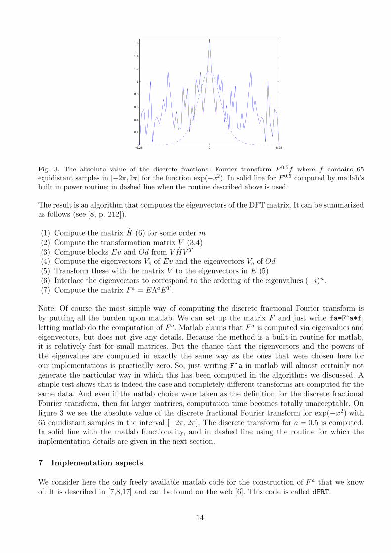
Fig. 3. The absolute value of the discrete fractional Fourier transform F 0.5f where f contains 65equidistant samples in [−2π, 2π] for the function exp(−x2). In solid line for F 0.5 computed by matlab’sbuilt in power routine; in dashed line when the routine described above is used.

The result is an algorithm that computes the eigenvectors of the DFT matrix. It can be summarizedas follows (see [8, p. 212]).

(1) Compute the matrix H (6) for some order m(2) Compute the transformation matrix V (3,4)(3) Compute blocks Ev and Od from V HV T

(4) Compute the eigenvectors Ve of Ev and the eigenvectors Vo of Od(5) Transform these with the matrix V to the eigenvectors in E (5)(6) Interlace the eigenvectors to correspond to the ordering of the eigenvalues (−i)n.(7) Compute the matrix F a = EΛaET .

Note: Of course the most simple way of computing the discrete fractional Fourier transform isby putting all the burden upon matlab. We can set up the matrix F and just write fa=F^a*f,letting matlab do the computation of F a. Matlab claims that F a is computed via eigenvalues andeigenvectors, but does not give any details. Because the method is a built-in routine for matlab,it is relatively fast for small matrices. But the chance that the eigenvectors and the powers ofthe eigenvalues are computed in exactly the same way as the ones that were chosen here forour implementations is practically zero. So, just writing F^a in matlab will almost certainly notgenerate the particular way in which this has been computed in the algorithms we discussed. Asimple test shows that is indeed the case and completely different transforms are computed for thesame data. And even if the natlab choice were taken as the definition for the discrete fractionalFourier transform, then for larger matrices, computation time becomes totally unacceptable. Onfigure 3 we see the absolute value of the discrete fractional Fourier transform for exp(−x2) with65 equidistant samples in the interval [−2π, 2π]. The discrete transform for a = 0.5 is computed.In solid line with the matlab functionality, and in dashed line using the routine for which theimplementation details are given in the next section.

7 Implementation aspects

We consider here the only freely available matlab code for the construction of F a that we knowof. It is described in [7,8,17] and can be found on the web [6]. This code is called dFRT.

14

First of all, to compare the result of the discrete fractional Fourier transform, we multiply thegiven vector f with the transform matrix SF aS where S represents here the cyclic shift matrixthat can be implemented as described in section 4.2.

To compute the discrete fractional Fourier transform, we have to compute the transformationmatrix as described in the previous section, and then multiply the given vector with this matrix.The computational complexity is O(n2), which is higher than for the fast approximate fractionalFourier transform. The larger part of the computation time goes to the construction of the eigen-vectors. These eigenvectors depend only on the size N and the order of approximation used. Thusif we want to compute the discrete fractional Fourier transform F af for a sequence of values ofa, then we have to compute the vectors E only once because F a = EΛaET . In the routine dFRT

this is solved in an ingenious way. The matrix of eigenvectors E and the approximation order pare stored as global variables. If the new size N of f and the new approximation order are equalto the size of the global matrix E and the global order p respectively, then the global matrix E isused again and is not recomputed.

When very high orders of approximation are used, like say m = N/2 and N large, then thecomputation of the factor (k!)2/(2k)! may cause overflow when the results (k!)2 and (2k)! arecomputed separately. That can be avoided when this coefficient is evaluated as

1

1· 1

2· 2

3· 2

4· · · k

2k − 1· k2k.

However, as the experiments show, taking these very high orders does not pay the effort.

The rest of the algorithm is a straightforward implementation of the method described in theprevious section. In dFRT, some of the steps are implemented in different function subroutineswhich are mostly avoided in our version. We also use the matlab toeplitz to construct thecirculant matrices.

Also for the computation of the eigenvalue decomposition of the blocks Ev and Od, the matlabroutine eig is used. This returns eigenvalues (and hence also the eigenvectors) in reverse order ofwhat is needed for the matrix E. A simple fliplr will place the vectors in the correct order. Theinterlacing operation to give the ordered columns of the matrix E can be done in the first placeon the indices as well.

One final remark. If you want to compute the DFRFT as fa = F af = EΛaETf , then the mutiplic-ation of the N ×N matrix F a with the vector f requires O(N 2) operations. However, computingF a = EΛaET , given E and Λa requires O(N 3) operations. Thus if only one DFRFT has to becomputed, it is more efficient to compute fa = E(Λa(ETf)). Multiplication with ET requiresO(N 2) operations, multiplication with Λa another O(N) and finally the multiplication with E isagain O(N 2), which is cheaper than first evaluating F a.

8 Discrete vs. continuous eigenvectors

One way of measuring how well the discrete transform approximates the continuous transformis by comparing the continuous Gauss-Hermite functions ψn with the corresponding eigenvectorsof F . A careful mathematical analysis for which we refer to the literature [7,8,18,17] reveals thatwhen ordered appropriately, the interlacing in step 6 of our algorithm in section 6 corresponds to

15

ordering the eigenvectors according to their number of zero crossings. That implies for examplethat the evens and odds will interlace. However, in view of the size of the blocks Ev and Od,it turns out that for N even, there is no eigenvector with N − 1 zero crossings and for N odd,there is no eigenvector with N zero crossings. Since the Gauss-Hermite function ψn has exactly nzero crossings, it is clear which eigenvector should approximate which ψn. More precisely, one canprove the following

Theorem 5 Let ψn be the Gauss-Hermite functions and let En be the eigenvector with n zerocrossings for the N ×N discrete Fourier transform matrix F .For N even, define the vector with N + 1 entries as

en = [En(N/2 + 2), . . . , En(N), En(1), . . . , En(N/2 + 2)]T .

Then, with proper normalization, it will contain approximations of the sample values in the vector

Ψn = [ψn(xk) : k = −N/2, . . . , N/2]T , xk = k√

2π/(N + 1).

For N odd, define the vector with N entries

en = [EN((N + 3)/2), . . . , EN(N), EN(1), . . . , EN((N + 1)/2)]T .

Then, with proper normalization, it will contain approximations of the sample values in the vector

Ψn = [ψn(xk) : k = −(N − 1)/2, . . . , (N − 1)/2]T , xk = k√

2π/N.

The term approximation means that the vectors en will converge to the vectors Ψn as N → ∞.

For a more precise treatment see [4,3].Note that the eigenvectors are supposed to be normalized, but even then, they are only definedup to a sign. For the definition of the discrete fractional Fourier transform, this sign is of noimportance because F a = EΛaET , and the sign does not matter.

The approximation becomes worse as n approaches N . We have illustrated this in figure 4. Thefunctions ψn are plotted in solid lines, the sample values Ψn are indicated by a cross and theapproximate vectors en are plotted with circles (and joined by a dashed line). In this figure, theapproximation order used for the matrix H is 2 (m = 1). For a larger N , the order does make adifference. For example in figure 5 we have plotted the case N = 100, and n = 30, on the left form = 1 and on the right for m = 20. It can be observed that the eigenvector of F has extremevalues for m = 1 at the beginning and the end, while for m = 20, these values are pulled towardszero, so that they give better approximants.

9 Other definitions of the DFRFT

Many other definitions of the discrete fractional Fourier transform do exist [2,21,22,5], but theyhave several theoretical disadvantages. For example the fast approximate fractional Fourier trans-form that we have discussed before is not a unitary operator like the discrete transform as definedabove is.

16

−6 −4 −2 0 2 4 6−1

−0.8

−0.6

−0.4

−0.2

0

0.2

0.4

0.6

0.8

1n = 2, N = 10

−5 −4 −3 −2 −1 0 1 2 3 4 5

−0.8

−0.6

−0.4

−0.2

0

0.2

0.4

0.6

0.8

n = 2, N = 100

−6 −4 −2 0 2 4 6−1

−0.8

−0.6

−0.4

−0.2

0

0.2

0.4

0.6

0.8

1n = 8, N = 10

−5 −4 −3 −2 −1 0 1 2 3 4 5

−0.8

−0.6

−0.4

−0.2

0

0.2

0.4

0.6

0.8

n = 8, N = 100

Fig. 4. The continuous Gauss-Hermite functions (solid line) sampled at equidistant points (+) and theeigenvectors (o) of the discrete FRFT matrix. On the left for 10 samples, on the right for 100 samples.On top for ψ2, at the bottom for ψ8.

−10 −5 0 5 10−1

−0.8

−0.6

−0.4

−0.2

0

0.2

0.4

0.6

0.8

1n = 30, N = 51

−10 −5 0 5 10−1

−0.8

−0.6

−0.4

−0.2

0

0.2

0.4

0.6

0.8

1n = 30, N = 51

Fig. 5. The continuous Gauss-Hermite functions (solid line) sampled at equidistant points (+) and theeigenvectors (o) of the discrete FRFT matrix for 100 samples, on the right for 100 samples. On the leftfor m = 1, and on the right for m = 20.

Another approach similar to the previous one is described in [18]. The idea is the following. Sincethe eigenvectors of the discrete Fourier transform matrix F are approximated by the samples of theGauss-Hermite eigenfunctions, it is proposed here that the vectors Ψn that were introduced in theprevious sections are projected onto the corresponding eigenspaces. There are only 4 eigenspaces:Ek, k = 0, 1, 2, 3 corresponding to the eigenvalues (−i)k, k = 0, 1, 2, 3. Because the eigenspacescorresponding to different eigenvalues will be orthogonal, it suffices to orthogonalize the projectionswithin their eigenspaces. Some special care has to be taken in the case of a signal length N thatis even, because then there is some jump in the sequence of eigenvalues, because the eigenvaluesare (−i)k, k = 0, . . . , N − 2, N − 1 for N odd and (−i)k, k = 0, . . . , N − 2, N for N even. So weuse the eigenvectors Ek with k zero crossings as defined in the routine dFRFT and the vectors of

17

corresponding sample values Ψk for example for N = 10, the spaces are spanned by the vectors

E0 E0, E4, E8

E1 E1, E5

E2 E2, E6, E10

E3 E3, E7

On the other hand, the following vectors are to be projected on the eigenspaces indicated

E0 Ψ0,Ψ4,Ψ8

E1 Ψ1,Ψ5

E2 Ψ2,Ψ6,Ψ10

E3 Ψ3,Ψ7

Our implementation uses similar tricks as in the case of dFRFT. We remark that the straightforwardcomputation of the Gauss-Hermite functions in their unnormalized form easily leads to overflowsince the hermite polynomials are growing very fast. Therefore a renormalization was implementedto avoid overflow and underflow.

Clearly, the extra projections and orthogonalizations needed require some extra computer time.On the other hand, the resulting eigenvectors that are used are much closer to the sample values ofthe continuous Gauss-Hermite functions. We give in figure 6 the analogs of figure 4, which showsthat there is a better correspondence.

Also the MIMO system implementation discussed in [10] is just a general setting to split thesignal into M disjunct blocks and process these blocks in parallel by a filter bank so that on amultiprocessor machine, the transform is computed faster, but this does not essentially changethe result.

Yet another implementation is proposed in [24]. However, this requires the precomputation of allthe fractional transforms xn = F bnf with b = 4/N if the signal has length N . This is only justifiedin very particular applications, but rather inefficient for a general purpose routine.

10 Discrete vs. fast approximate transform

In figure 7 we see the absolute value of the fractional Fourier transform of cos(x) where x =0 : 0.02 : 2π. The discrete transform is drawn in solid line, the fast approximate transform isdrawn in dashed line. This figure illustrates a general observation: the fast approximate transformoscillates more near the boundaries, while the discrete transform oscillates more in the middleof the interval if the approximation order is too small (i.e., if m is small). However for a largerm, the approximation of the fast approximate transform is much better, as can be observed inthe right plot. As could have been predicted from the previous section, the approximation of theGauss-Hermite functions by the eigenvectors of the discrete transform matrix not being very goodnear the boundaries when the number of zero crossings is high, it is also generally true that for

18

−4 −3 −2 −1 0 1 2 3 4−1

−0.8

−0.6

−0.4

−0.2

0

0.2

0.4

0.6

0.8

1n=2

−6 −4 −2 0 2 4 6−0.8

−0.6

−0.4

−0.2

0

0.2

0.4

0.6

0.8

n= 2

−4 −3 −2 −1 0 1 2 3 4−0.8

−0.6

−0.4

−0.2

0

0.2

0.4

0.6

0.8

1n= 8

−6 −4 −2 0 2 4 6

−0.6

−0.4

−0.2

0

0.2

0.4

0.6

0.8

n= 8

Fig. 6. The continuous Gauss-Hermite functions (solid line) sampled at equidistant points (+) and theeigenvectors (o) of the discrete FRFT matrix using DFPei. On the left for 10 samples, on the right for100 samples. On top for ψ2, at the bottom for ψ8.

0 1 2 3 4 5 6

0.2

0.4

0.6

0.8

1

1.2

1.4

0 1 2 3 4 5 6

0.2

0.4

0.6

0.8

1

1.2

1.4

a = 0.5

Fig. 7. Absolute value of F0.5(cos(x)) (dashed) and of F 0.5(cos(x)) (solid), where x = 0 : 0.02 : 2π. Onthe left with m = 2, on the right with m = 30.

most values of a, the discrete fractional Fourier transform does not approximate very well the fastapproximate fractional Fourier transform near the boundaries. If N is large, then a high order ofapproximation, i.e., taking relatively large values of m will help.

The discrete transform algorithm is considerably slower than the fast approximate transform. Thecomputation of the eigenvectors is the most time consuming. Therefore the trick of saving theeigenvectors avoiding recomputation for different values of a when N and m remain the same is aconsiderable saving of computer time.

A plot of the DFRFT with the Pei or Candan algorithms gives only minor differences. See figure 8.Note the irregular behaviour of the Pei approximant near the boundary.

Since the discrete fractional sine and cosine transform algorithms as described in [20] are essentiallyobtained by taking as eigenvectors half of the even or odd eigenvectors of the discrete fractionalFourier transform matrix that has twice the size of the signal, it should be clear that implementa-

19

0 1 2 3 4 5 6

0.2

0.4

0.6

0.8

1

1.2

1.4

Fig. 8. The fast approximate fractional Fourier transform F 0.5(cosx) where x = 0 : 0.02 : 2π, i.e.,N = 315 (dash-dotted line), and the discrete transform corresponding to the DFpei code (solid line) andthe discrete transform corresponding to the code Disfrft (dashed line). The order of approximation usedis p = N/2.

Fig. 9. On the left, an image that is contaminated by a chirp which has sweep rate 0.6 in the x-directionand 0.3 in the y-direction. When the separable two-dimensional discrete fractional Fourier transform isapplied with the appropriate orders, then the chirp will be transformed in a delta-function. It is theneasily identified and removed. After back transforming the clean image is reconstructed as on the right.

tions for these transforms are directly obtained from the implementation of the discrete fractionalFourier transform that we have discussed.

11 Two-dimensional transform

Although there exists a definition of an non-separable two-dimensional fractional Fourier trans-form, the easiest application is a tensor product type of two-dimensional fractional Fourier trans-form by applying subsequently the one-dimensional transform to the rows and the columns ofthe image. As an example, we superposed a chirp noise on an image as can be seen in the leftof figure 9. After the appropriate one-dimensional discrete fractional Fourier transforms on therows and the columns, the chirp is transformed to a delta-function. This can be seen in figure 10,where we have plotted a mesh for the rows and columns in the neighborhood of the delta-function.Even though the noise is hardly seen in the image, the peak clearly stands out and this identifies

20

100

110

120

130

140

70

80

90

100

1100

200

400

600

800

1000

1200

1400

1600

1800

Fig. 10. After the appropriate one-dimensional transforms on the rows and the columns of the image thechirp is transformed into a delta-function. The plot shows the neighborhood of the peak.

that the appropriate transformation has been made. After removal by replacing the peak by theaverage on the neighboring pixels, the image is back transformed and a clean image is found.

12 Conclusion

We have compared two existing routines for the computation of the fast approximate fractionalFourier transform and one routine for the discrete fractional Fourier transform. We studied in detailthe different steps of the implementation and propose our own implementaion as an alternativethat overcomes some of the restrictions. We also test an implementation for the discrete fractionalFourier transform, compare the results of the discrete and the fast approximate transforms anddescribe our own implementation. It is compared with another algorithm of Pei which is baed onorthogonal projections. The extra computational effort did not seem to be worthwhile in general.Adaptations of our implementation for obtaining discrete sine or cosine transforms are easy.

Matlab versions of our implementations are available on the website

www.cs.kuleuven.ac.be/~nalag/research/software/FRFT/

References

[1] L.B. Almeida. The fractional Fourier transform and time-frequency representation. IEEE Trans.

Sig. Proc., 42:3084–3091, 1994.

[2] N.M. Atakishiyev, L.E. Vicent, and K.B. Wolf. Continuous vs. discrete fractional Fourier transform.J. Comput. Appl. Math., 107:73–95, 1999.

[3] L. Barker. The discrete fractional Fourier transform and Harper’s equation. Mathematika, 47(1-2):281–297, 2000.

[4] L. Barker, C. Candan, T. Hakioglu, M.A. Kutay, and H.M. Ozaktas. The discrete harmonic oscillator,Harper’s equation, and the discrete Fractional Fourier Transfom. J. Phys. A, 33:2209–2222, 2000.

21

[5] G. Cariolaro, T. Erseghe, P. Kraniauskas, and N. Laurenti. Multiplicity of fractional Fouriertransforms and their relationships. IEEE Trans. Sig. Proc., 48(1):227–241, 2000.

[6] C. Candan. dFRT: The discrete fractional Fourier transform, 1996. A matlab programwww.ee.bilkent.edu.tr/~haldun/dFRT.m.

[7] C. Candan. The discrete Fractional Fourier Transform. MS Thesis, Bilkent University, Ankara,1998.

[8] C. Candan, M.A. Kutay, and H.M. Ozaktas. The discrete Fractional Fourier Transform. IEEE

Trans. Sig. Proc., 48:1329–1337, 2000.

[9] E.U. Condon. Immersion of the Fourier transform in a continuous group of functional transformations.Proc. National Academy Sciences, 23:158–164, 1937.

[10] D.F. Huang and B.S. Chen. A multi-input-multi-output system approach for the computation ofdiscrete fractional Fourier transform. Signal Processing, 80:1501–1513, 2000.

[11] H. Kober. Wurzeln aus der Hankel- und Fourier und anderen stetigen Transformationen. Quart. J.

Math. Oxford Ser., 10:45–49, 1939.

[12] M.A. Kutay. fracF: Fast computation of the fractional Fourier transform, 1996.www.ee.bilkent.edu.tr/~haldun/fracF.m.

[13] A.C. McBride and F.H. Kerr. On Namias’s fractional Fourier transforms. IMA J. Appl. Math.,39:159–175, 1987.

[14] V. Namias. The fractional order Fourier transform and its application in quantum mechanics. J.

Inst. Math. Appl., 25:241–265, 1980.

[15] J. O’Neill. DiscreteTFDs:a collection of matlab files for time-frequency analysis, 1999.ftp.mathworks.com/pub/contrib/v5/signal/DiscreteTFDs/.

[16] H.M. Ozaktas, M.A. Kutay, and G. Bozdagi. Digital computation of the fractional Fourier transform.IEEE Trans. Sig. Proc., 44:2141–2150, 1996.

[17] H.M. Ozaktas, Z. Zalevsky, and M.A. Kutay. The fractional Fourier transform. Wiley, Chichester,2001.

[18] S.-C. Pei, M.-H. Yeh, and C.-C. Tseng. Discrete fractional Fourier-transform based on orthogonalprojections. IEEE Trans. Sig. Proc., 47(5):1335–1348, 1999.

[19] S.C. Pei and M.H. Yeh. Improved discrete fractional Fourier transform. Optics Letters, 22:1047–1049,1997.

[20] S.C. Pei and M.H. Yeh. The discrete fractional cosine and sine transforms. IEEE Trans. Sig. Proc.,49:1198–1207, 2001.

[21] M.S. Richman, T.W. Parks, and R.G. Shenoy. Understanding discrete rotations. In Proc. IEEE Int.

Conf. Acoust. Speech, Signal Process., 1997.

[22] B. Santhanam and J.H. McClellan. The discrete rotational Fourier transform. IEEE Trans. Sig.

Proc., 44:994–998, 1996.

[23] N. Wiener. Hermitian polynomials and Fourier analysis. J. Math. Phys., 8:70–73, 1929.

[24] M.H. Yeh and S.C. Pei. A method for the discrete fractional Fourier transform computation. IEEE

Trans. Sig. Proc., 51(3):889–891, 2003.

22