Grenoble INP – ENSIMAGÉcole Nationale Supérieure d’ Informatique et de Mathématiques Appliquées

Final master project report

The Australian University - RSISEResearch School of Information Sciences and Engineering

Computation of the Spatial Impulse Responsefor Ultrasonic Fields on the Graphics

Processing Units (GPU)

Luna Florian3rd year – Option IRV

21st February 2010 – 21st August 2010

RSISE-ANU ANU supervisorNorth Road - Acton Shams Ramtin, Richard HartleyRSISE Building 115 FIB supervisor2601 Canberra - ACT Australia Pere Brunet

2

ContactsStudent

Florian LunaPhone : (+33) 632211964Adress : Quartier le Plan - Le Grand Barsan - 84110 Vaison-la-RomaineEmail : Florian.Luna@gmail.com

Lab Supervisors

Ramtin ShamsEmail : Ramtin.Shams@anu.edu.auPhone : +61 2 6125 8612Fax : +61 2 6125 8660

Richard HartleyEmail : Richard.Hartley@anu.edu.auPhone : (+61) 2 6125 8668Fax : (+61) 2 6125 8660

Address of the RSISEANU College of Engineering & Computer ScienceRSISE Building 115, North RoadThe Australian National UniversityCanberra ACT 0200, Australia

FIB tutor

Pere Brunetpere@lsi.upc.edu

3

AknowledgementsFirst of all, I would like to thank Ramtin Shams for all his support during my internship. Hehelped me not only for my project but also for settling down in Canberra, which was not an easytask. I would like also to thank Parastoo Sadeghi for her help during my internship. I am verythankful for Richard Hartley who supervised me and contributed to bring me in Canberra.

I am also very thankful for the support of my ENSIMAG tutor Marie-Paule Cani, who super-vised me all this year. And my final thank will be to the International Relations Office, AurélieBonachera and Marianne Genton who made an outstanding work.

4 CONTENTS

Contents1 Summary 6

2 Internship presentation 62.1 Introduction . . . . . . . . . . . . . . . . . . . . . . . . . . . . . . . . . . . . . 62.2 The Research School of Information Science and Engineering . . . . . . . . . . 62.3 My supervisors . . . . . . . . . . . . . . . . . . . . . . . . . . . . . . . . . . . 62.4 Contributions . . . . . . . . . . . . . . . . . . . . . . . . . . . . . . . . . . . . 72.5 Summary and key words . . . . . . . . . . . . . . . . . . . . . . . . . . . . . . 7

3 Background 93.1 Overview of Wave-based Ultrasound Modeling . . . . . . . . . . . . . . . . . . 9

3.1.1 Ultrasound Medical Imaging . . . . . . . . . . . . . . . . . . . . . . . . 93.1.2 Transducers . . . . . . . . . . . . . . . . . . . . . . . . . . . . . . . . . 10

3.2 The Spatial Impulse Response . . . . . . . . . . . . . . . . . . . . . . . . . . . 103.3 Overview of GPU Programming on CUDA . . . . . . . . . . . . . . . . . . . . 12

3.3.1 Architecture of a CUDA Capable Processor . . . . . . . . . . . . . . . . 133.3.2 Programming model . . . . . . . . . . . . . . . . . . . . . . . . . . . . 133.3.3 Goals of a CUDA programmer . . . . . . . . . . . . . . . . . . . . . . . 15

3.4 Objectives after analysing the problem . . . . . . . . . . . . . . . . . . . . . . . 15

4 Development of the application 164.1 About UltraCuda . . . . . . . . . . . . . . . . . . . . . . . . . . . . . . . . . . 164.2 Chronology of the developement . . . . . . . . . . . . . . . . . . . . . . . . . . 164.3 Architecture of the application . . . . . . . . . . . . . . . . . . . . . . . . . . . 16

4.3.1 Multi-threading . . . . . . . . . . . . . . . . . . . . . . . . . . . . . . . 174.4 Computing the Spatial Impulse Response for one transducer element . . . . . . . 17

4.4.1 Efficient algorithm for computing the intersection between simple poly-gons and a circle . . . . . . . . . . . . . . . . . . . . . . . . . . . . . . 17

4.4.2 Initializing the algorithm . . . . . . . . . . . . . . . . . . . . . . . . . . 184.4.3 Exploring all the edges . . . . . . . . . . . . . . . . . . . . . . . . . . . 194.4.4 Special cases, tangents and corners . . . . . . . . . . . . . . . . . . . . 194.4.5 Geometric elements . . . . . . . . . . . . . . . . . . . . . . . . . . . . 19

4.5 Preprocessing of the data . . . . . . . . . . . . . . . . . . . . . . . . . . . . . . 204.5.1 First algorithm . . . . . . . . . . . . . . . . . . . . . . . . . . . . . . . 214.5.2 Second algorithm . . . . . . . . . . . . . . . . . . . . . . . . . . . . . . 21

5 Results 225.1 Validation . . . . . . . . . . . . . . . . . . . . . . . . . . . . . . . . . . . . . . 22

5.1.1 Comparaison with Field II . . . . . . . . . . . . . . . . . . . . . . . . . 225.1.2 Testing different kinds of configuration . . . . . . . . . . . . . . . . . . 225.1.3 Comparaison with Field II . . . . . . . . . . . . . . . . . . . . . . . . . 24

CONTENTS 5

5.2 Performances of the application . . . . . . . . . . . . . . . . . . . . . . . . . . 265.2.1 Timing by varying the number of aperture . . . . . . . . . . . . . . . . . 265.2.2 Timing by varying the number of points . . . . . . . . . . . . . . . . . . 28

5.3 Incoming tasks and possible improvments . . . . . . . . . . . . . . . . . . . . . 28

6 Conclusions 296.1 About UltraCuda . . . . . . . . . . . . . . . . . . . . . . . . . . . . . . . . . . 296.2 Personal Experience . . . . . . . . . . . . . . . . . . . . . . . . . . . . . . . . . 29

7 Appendix 317.1 Résumé du stage . . . . . . . . . . . . . . . . . . . . . . . . . . . . . . . . . . 317.2 Geforce GTX 295 . . . . . . . . . . . . . . . . . . . . . . . . . . . . . . . . . . 317.3 Some Matlab scripts . . . . . . . . . . . . . . . . . . . . . . . . . . . . . . . . 32

6 2 INTERNSHIP PRESENTATION

1 Summary

2 Internship presentation

2.1 Introduction

I chose studying computer science at ENSIMAG because I have always been fascinated by sim-ulating and vizualising our surrounding world through computer devices. That interest led me tochoose the Image Processing and Virtual Reality speciality at the Ensimag and then the Interfaceand Vizualisation speciality at the Polytechnic University of Catalunya. The applications of thistopic are growing up and medical imaging is one of the most important. Improving the medicaltechnology by using computer knowledge has always appealed to me. Furthermore, physics ofsound is something that I am very interested in due to my musical background. Choosing thatinternship was not difficult as it was a mix of what I had studied before and personal interests.

The report falls into the following parts. The first one is a presentation of the internship. Itis then followed by an analysis of the problem we want to simulate and a brief presentation ofCUDA (Computer Unified Architecture). The solution and the development of the applicationare then detailed. The validity and the results are presented. The report comes to an end with aconclusion about the project achievement and the personal experience gained during the trainee.

2.2 The Research School of Information Science and Engineering

I did my internship at the Research School of Information Sciences and Engineering (RSISE).The RSISE is one of twelve research schools at ANU and was established on 1 January 1994. Itevolved from the Department of Systems Engineering (1981) within the then Research School ofPhysical Sciences and Engineering (RSPhysSE) and the Computer Sciences Laboratory (1988)also within RSPhysSE.

2.3 My supervisors

My two supervisors were Dr Ramtin Shams and Pr Richard Hartley.

Dr. Shams is a Fellow (senior lecturer) at the School of Engineering at the Australian Na-tional University (ANU). He received his B.E. and M.E. degrees in electrical engineering fromSharif University of Technology, Tehran, and his PhD in biomedical engineering from ANU.

He received an Australian Postdoctoral (APD) Fellowship in 2009 and was the recipient of aFulbright scholarship in 2008. He has more than ten years of industry experience in the ICT sec-tor and worked as the CTO of GPayments Pty. Ltd between 2001 to 2007. His research interestsinclude medical image analysis, high performance computing, and wireless communications.

2.4 Contributions 7

Prof. Richard Hartley is the Head of Computer Vision and Robotics group at ANU. Prof.Hartley is a Fellow of Australian Academy of Science and an IEEE Fellow. From 1984 until2001 he was a member of the research staff at General Electric R&D Center in New York wherehis research involved Computer Vision and Medical Imaging.

He has 34 patents including 9 in the area of medical imaging. He has published more than200 papers. He is a highly cited author and his book ’Multiple View Geometry in ComputerVision’ is the main reference in this area. Prof. Hartley is on the editorial board of IJCV and isthe General chair of ICCV 2011. He is the recipient of GE’s Dushman award in 1990 (highestrecognition for research at GE).

2.4 ContributionsThe series of papers [1],[2] and [3] use a simple ray-based model for ultrasound simulation andachieve real-time performance. We want not only to accelerate the simlation by using the GPUbut also to use a wave-based model of ultrasound based on the concepts of linear acoustics andspatial impulse response.

More precisely, the implementation has been done in C++/CUDA (Compute Unified DeviceArchitecture). CUDA gives developers access to the native instruction set and memory of theparallel computational elements in CUDA GPUs. We present here an implementation of thecomputation of the spatial impulse response for polygonal aperture transducers.

We have used an incremental algorithm more suited to the GPU than the one proposed in [4].The final contribution is the application UltraCuda, developed on C++/CUDA which computesthe spatial impulse response of transducer made of many simple aperture.

2.5 Summary and key wordsKey words : Simulation, Real-Time, Ultrasound, Spatial Impulse Response, GPU.

The goal of the internship was to develop a linear wave-based simulation of ultrasonic fields.The theory was based on the Tupholme-Stepanishen formalism explained in the Jensen course forcalculating pulsed ultrasound field. The Field II Simulation Program developed at the TechnicalUniversity of Denmark does that simulation but the program runs slowly due to the fact that itruns only on the CPU. It is getting older as it was released in 1994. Designing an algorithm andimplementing an application which parallelizes the computation of the spatial impulse responseon the GPU were the main goal of my internship. More precisely, my tasks were to

• Become familiarized with ultrasound physics and GPU programming.

• Have a first go with the simulation through Matlab.

• Devise an algorithm suited to GPU programming.

8 2 INTERNSHIP PRESENTATION

• Develop an application able to simulate different kinds of configurations and the corre-sponding data structures. The application is called through Matlab commands but all thesimulation are made with C++/CUDA programming.

• Verify the validity and time the execution of our implementation.

9

3 Background

3.1 Overview of Wave-based Ultrasound Modeling

Introduction

Wave-based ultrasound modeling is necessary to improve and to optimize ultrasound imaging.Indeed, by simulating the behaviour of ultrasound devices, it is then possible to design ultrasoundimaging devices at a lower cost. The overview of what is wave-based ultrasound will fall intothree parts. First, we give an introduction about the different aspects of ultrasound imaging. Thenwe present what a transducer is. To finish, we present the model we have used for the simulation.

3.1.1 Ultrasound Medical Imaging

Ultrasound imaging remains a very convenient modality. Indeed, it is real-time with high tempo-ral resolution and harmless. Furthermore, ultrasound devices are relatively cheap and portable.The main drawback is the image quality as you can see in the figure 2.

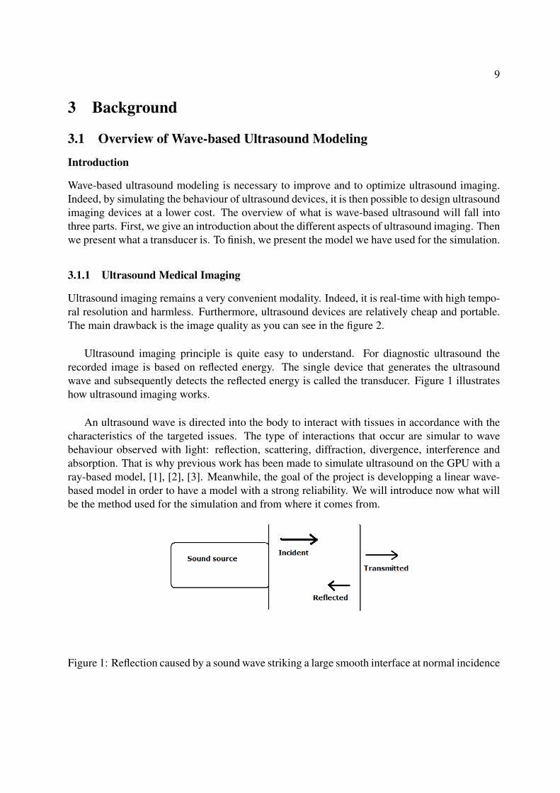
Ultrasound imaging principle is quite easy to understand. For diagnostic ultrasound therecorded image is based on reflected energy. The single device that generates the ultrasoundwave and subsequently detects the reflected energy is called the transducer. Figure 1 illustrateshow ultrasound imaging works.

An ultrasound wave is directed into the body to interact with tissues in accordance with thecharacteristics of the targeted issues. The type of interactions that occur are simular to wavebehaviour observed with light: reflection, scattering, diffraction, divergence, interference andabsorption. That is why previous work has been made to simulate ultrasound on the GPU with aray-based model, [1], [2], [3]. Meanwhile, the goal of the project is developping a linear wave-based model in order to have a model with a strong reliability. We will introduce now what willbe the method used for the simulation and from where it comes from.

Figure 1: Reflection caused by a sound wave striking a large smooth interface at normal incidence

10 3 BACKGROUND

Figure 2: Application of ultrasound imaging, echography of a baby

3.1.2 Transducers

As explained before, a transducer is a device able to convert electricity energy into ultrasoundenergy and vice versa. This phenomenon is explained by the piezoelectric effect. A single ele-ment transducer is a planar geometric surface which vibrates. We will suppose that the vibrationis homogeneous on the whole surface, even if it is apodized in reality.

A transducer can be made of multiple simple transducers arranged into a linear array forexample. With that configuration, you can set a delay for each aperture and so on having thepossibility to modify the shape of the ultrasonic field created.

3.2 The Spatial Impulse Response

Our simulation of the ultrasound wave is based on the same model as the one used in the Fieldprogram. It relies on the concept of spatial impulse response developed by Tuphole and Stephan-ishen [4]. It is inherited from the electrical linear system theory. Indeed, a linear electrical systemis fully characterized by its impulse response. The output of any y(t) to any kind of input signalx(t) is given by

y(t) = h(t) ? x(t) =

∫ +∞

−∞h(θ)x(t− θ) dθ (1)

where h(t) is the impulse response and ? the convolution operator. The transfer function ofthe system is the Fourier transform of the impulse response.

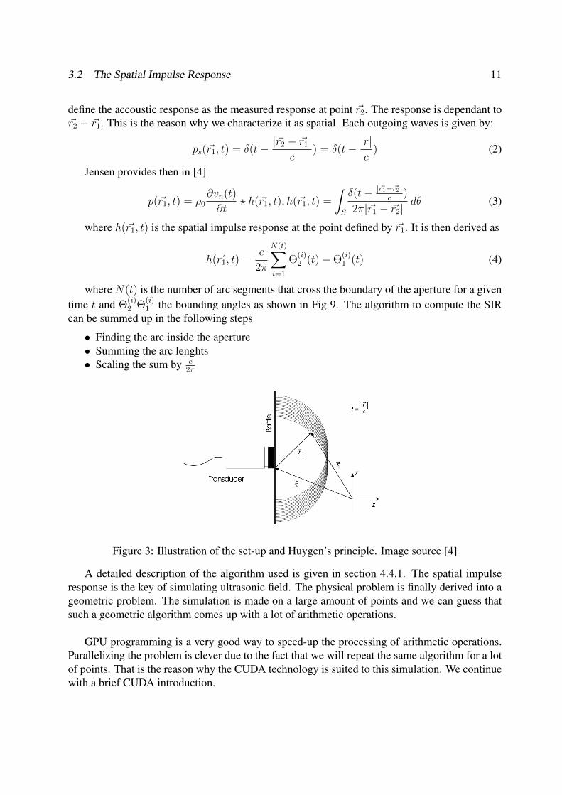
Fig 3 illustrates the basic set-up of a linear acoustic system. The transducer is rigid and set atposition ~r2. It radiates at the sound speed c into a homogeneous medium of density ρ0. Huygen’sprinciple assimilates each point of a radiating surface as the origin of an outgoing spherical wave.An excitation of the transducer with a Dirac function (δ) will give rise to a pressure field. We

3.2 The Spatial Impulse Response 11

define the accoustic response as the measured response at point ~r2. The response is dependant to~r2 − ~r1. This is the reason why we characterize it as spatial. Each outgoing waves is given by:

ps(~r1, t) = δ(t− |~r2 − ~r1|c

) = δ(t− |r|c

) (2)

Jensen provides then in [4]

p(~r1, t) = ρ0∂vn(t)

∂t? h(~r1, t), h(~r1, t) =

∫S

δ(t− |~r1−~r2|c

)

2π|~r1 − ~r2|dθ (3)

where h(~r1, t) is the spatial impulse response at the point defined by ~r1. It is then derived as

h(~r1, t) =c

2π

N(t)∑i=1

Θ(i)2 (t)−Θ

(i)1 (t) (4)

where N(t) is the number of arc segments that cross the boundary of the aperture for a giventime t and Θ

(i)2 Θ

(i)1 the bounding angles as shown in Fig 9. The algorithm to compute the SIR

can be summed up in the following steps

• Finding the arc inside the aperture• Summing the arc lenghts• Scaling the sum by c

2π

Figure 3: Illustration of the set-up and Huygen’s principle. Image source [4]

A detailed description of the algorithm used is given in section 4.4.1. The spatial impulseresponse is the key of simulating ultrasonic field. The physical problem is finally derived into ageometric problem. The simulation is made on a large amount of points and we can guess thatsuch a geometric algorithm comes up with a lot of arithmetic operations.

GPU programming is a very good way to speed-up the processing of arithmetic operations.Parallelizing the problem is clever due to the fact that we will repeat the same algorithm for a lotof points. That is the reason why the CUDA technology is suited to this simulation. We continuewith a brief CUDA introduction.

12 3 BACKGROUND

Figure 4: Intersections of the projected spherical wave and the aperture. Image source [4]

3.3 Overview of GPU Programming on CUDA

Introduction

For more than two decades, standard microprocessors were based on a single central processingunit(CPU), such as the Intel Pentiun and AMD Opteron. Recently, the processor manufacturershave changed their strategy due to the lack of improvement in clock frequency and switched tomultiple processing units. Indeed, parallelization is an efficient way to increase the computa-tional capacity.

The graphic processing unit(GPU) such as the NVIDIA or ATI families were mainly usedfor graphic purposes. For example, GLSL is a C-style language for programming shaders whichreplaces some steps of the graphic pipeline. The power of GPU has never stopped increasing.Nowadays, GPUs are useful not only for graphic purposes but also general purpose arithmeticcomputing.

GPU has evolved into a highly parallel, multithread, manycore processor with high memorybandwith. That’s why it is well-suited to address problems that can be solved with data-parallelcomputations. The main idea of GPU programming is that data-parallel processing maps data el-ements to parallel processing threads. The same program will be executed for each data element.

One can compare the characteristics of the CPU and the GPU. For instance, an Intel Core2 (2.66GHz) provides 14.2 GFlops although a GeForce 9800 GTX (only 675 Mhz) provides420 GFlops. But the GPU is really efficient if used on a suitable problem. In November 2006,NVIDIA introduced CUDA which is a general purpose parallel architecture which solves manycomputational problems in a better way than the the CPU does.

3.3 Overview of GPU Programming on CUDA 13

3.3.1 Architecture of a CUDA Capable Processor

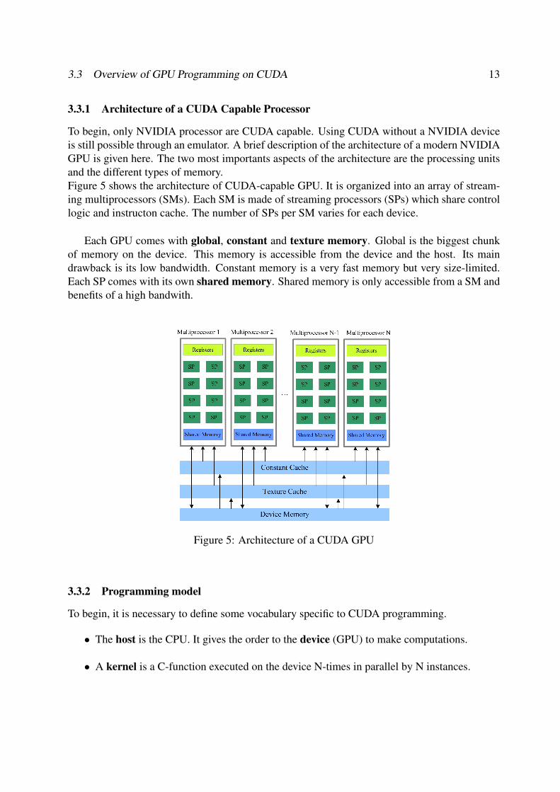
To begin, only NVIDIA processor are CUDA capable. Using CUDA without a NVIDIA deviceis still possible through an emulator. A brief description of the architecture of a modern NVIDIAGPU is given here. The two most importants aspects of the architecture are the processing unitsand the different types of memory.Figure 5 shows the architecture of CUDA-capable GPU. It is organized into an array of stream-ing multiprocessors (SMs). Each SM is made of streaming processors (SPs) which share controllogic and instructon cache. The number of SPs per SM varies for each device.

Each GPU comes with global, constant and texture memory. Global is the biggest chunkof memory on the device. This memory is accessible from the device and the host. Its maindrawback is its low bandwidth. Constant memory is a very fast memory but very size-limited.Each SP comes with its own shared memory. Shared memory is only accessible from a SM andbenefits of a high bandwith.

Figure 5: Architecture of a CUDA GPU

3.3.2 Programming model

To begin, it is necessary to define some vocabulary specific to CUDA programming.

• The host is the CPU. It gives the order to the device (GPU) to make computations.

• A kernel is a C-function executed on the device N-times in parallel by N instances.

14 3 BACKGROUND

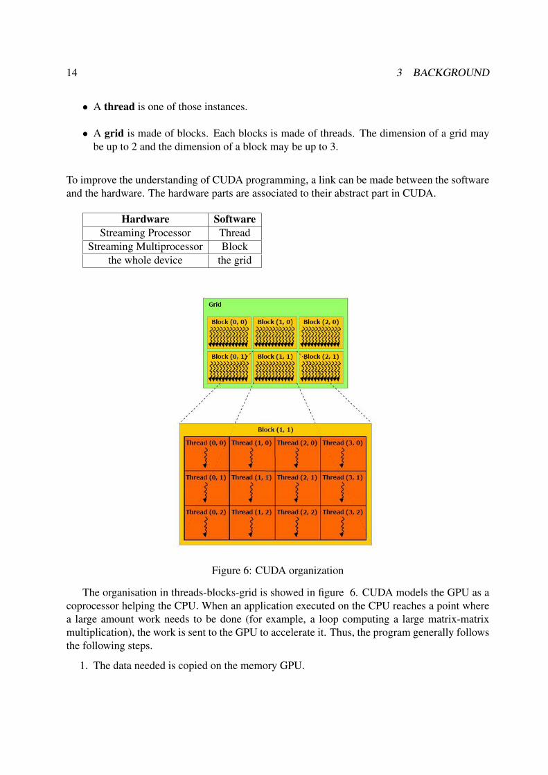
• A thread is one of those instances.

• A grid is made of blocks. Each blocks is made of threads. The dimension of a grid maybe up to 2 and the dimension of a block may be up to 3.

To improve the understanding of CUDA programming, a link can be made between the softwareand the hardware. The hardware parts are associated to their abstract part in CUDA.

Hardware SoftwareStreaming Processor Thread

Streaming Multiprocessor Blockthe whole device the grid

Figure 6: CUDA organization

The organisation in threads-blocks-grid is showed in figure 6. CUDA models the GPU as acoprocessor helping the CPU. When an application executed on the CPU reaches a point wherea large amount work needs to be done (for example, a loop computing a large matrix-matrixmultiplication), the work is sent to the GPU to accelerate it. Thus, the program generally followsthe following steps.

1. The data needed is copied on the memory GPU.

3.4 Objectives after analysing the problem 15

2. The programmer configures the size of the grid and the size of the blocks.3. The parallel computing is executed through a kernel on the GPU.4. Once the work finished, the result is copied back to the CPU and application continues.

3.3.3 Goals of a CUDA programmer

A CUDA program is not a trivial task. [8] gives the fundamental things to in CUDA. The priori-ties of a CUDA programer would be:

• Maximizing parallel execution• Optimizing memory usage to achieve maximum memory bandwidth• Optimizing instruction usage to achieve maximum instruction throughput

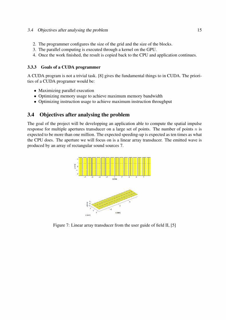
3.4 Objectives after analysing the problemThe goal of the project will be developping an application able to compute the spatial impulseresponse for multiple apertures transducer on a large set of points. The number of points n isexpected to be more than one million. The expected speeding-up is expected as ten times as whatthe CPU does. The aperture we will focus on is a linear array transducer. The emitted wave isproduced by an array of rectangular sound sources 7.

Figure 7: Linear array transducer from the user guide of field II, [5]

16 4 DEVELOPMENT OF THE APPLICATION

4 Development of the application

4.1 About UltraCudaUltraCuda is the name of the application we have implemented to solve the problem exposedbefore. The application is made for a Windows environment and Matlab is necessary to use it.First, we explain precisely how the problem can be parallelized. Then we present our algorithmwhich computes the spatial impulse response. To finish, we will deschribe the final applicationarchitecture. We briefly introduce now the working environment and then the steps of the devel-opment.

We have first used Matlab for testing the geometric algorithm. Indeed, it is quicker to set upa basic simulation on Matlab than in C++. It is then easy to debug and it is useful to test the algo-rithm. The debugging in C++ will be then about memory management on the host and the device.

Then, we have used Matlab to call the C++/CUDA function through a wrapper created withthe mex library. It is a convenient way to manipulate vector outside C and manipulating databefore sending them to our program. CUDA has been chosen for the multi threading. Even ifOpenCL can be used with other GPUs than the NVIDIA ones, CUDA remained very convenient.We had already a lot of helper and generic algorithms like reduction already implemented inCUDA and fully tested.

4.2 Chronology of the developementWe will sum up here the step of the development. The steps of the develoment were:

• Simulating the Spatial Impulse Response for a simple transducer on Matlab and visualizingthe results by different kinds of plottings.

• Discussing the architecture of the application and the data structure used

• Implementing the inititialisation of the algorithm.

• Designing algorithms suited to GPU computation.

• Implementing the new algorithm for a simple transducer.

• Implementing two versions of the simulation for multiple transducers.

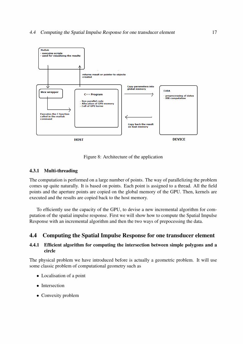
4.3 Architecture of the applicationThe program consists of a C++/CUDA program. All calculations are performed by the C++program and all the data is kept by the C++ program. All the massive parallel part of the codeare executed by CUDA. The C-function are called through a wrapper. The organisation of theprogram is shown on the figure 8.

4.4 Computing the Spatial Impulse Response for one transducer element 17

Figure 8: Architecture of the application

4.3.1 Multi-threading

The computation is performed on a large number of points. The way of parallelizing the problemcomes up quite naturally. It is based on points. Each point is assigned to a thread. All the fieldpoints and the aperture points are copied on the global memory of the GPU. Then, kernels areexecuted and the results are copied back to the host memory.

To efficiently use the capacity of the GPU, to devise a new incremental algorithm for com-putation of the spatial impulse response. First we will show how to compute the Spatial ImpulseResponse with an incremental algorithm and then the two ways of prepocessing the data.

4.4 Computing the Spatial Impulse Response for one transducer element4.4.1 Efficient algorithm for computing the intersection between simple polygons and a

circle

The physical problem we have introduced before is actually a geometric problem. It will usesome classic problem of computational geometry such as

• Localisation of a point

• Intersection

• Convexity problem

18 4 DEVELOPMENT OF THE APPLICATION

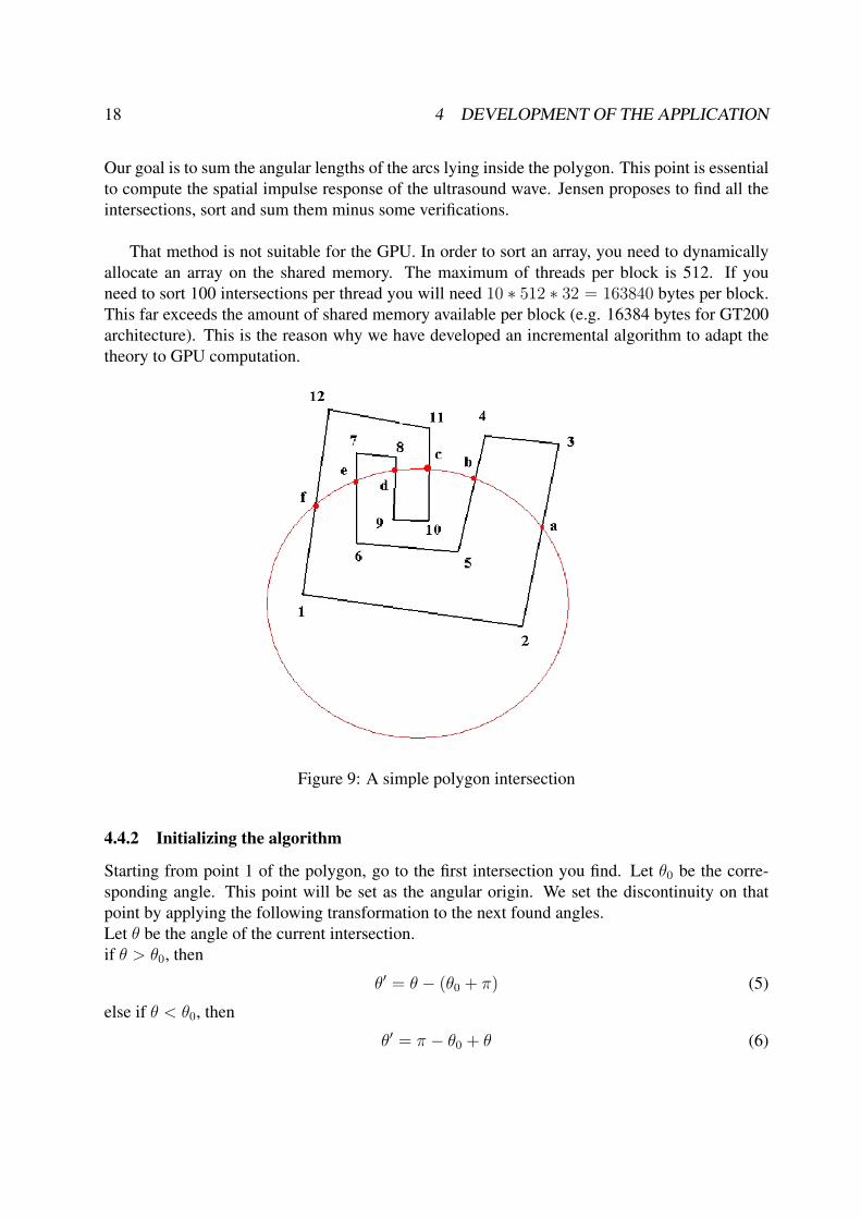
Our goal is to sum the angular lengths of the arcs lying inside the polygon. This point is essentialto compute the spatial impulse response of the ultrasound wave. Jensen proposes to find all theintersections, sort and sum them minus some verifications.

That method is not suitable for the GPU. In order to sort an array, you need to dynamicallyallocate an array on the shared memory. The maximum of threads per block is 512. If youneed to sort 100 intersections per thread you will need 10 ∗ 512 ∗ 32 = 163840 bytes per block.This far exceeds the amount of shared memory available per block (e.g. 16384 bytes for GT200architecture). This is the reason why we have developed an incremental algorithm to adapt thetheory to GPU computation.

Figure 9: A simple polygon intersection

4.4.2 Initializing the algorithm

Starting from point 1 of the polygon, go to the first intersection you find. Let θ0 be the corre-sponding angle. This point will be set as the angular origin. We set the discontinuity on thatpoint by applying the following transformation to the next found angles.Let θ be the angle of the current intersection.if θ > θ0, then

θ′ = θ − (θ0 + π) (5)

else if θ < θ0, then

θ′ = π − θ0 + θ (6)

4.4 Computing the Spatial Impulse Response for one transducer element 19

4.4.3 Exploring all the edges

We explore the polygon in the counterclockwise order.Let S be the sum of the arc lengths.Let P be the array of points of the polygon given in the counterclockwise order.Let n be the number of points in the polygon .Let sign be an integer whose value alternate between 1 and -1.Let θmin be the angle of the closest intersection to the first one intersection in the counterclock-wise order.

• To initialize the algorithm, Find the first intersection and keep the first angle θ0. For theother intersection angles, apply the transformation presented in the previous section.sign = −1;S = sign ∗ θ0;sign = −sign;

• Explore all the edge in counterclockwise order. For each edge, find the intersections. Ifthere are 2 intersections, proceed first with the closest intersection to the first point of theedge. Let θ be the corresponding angle after the transformation.S+ = sign ∗ θ;sign = −sign;if (θ − θ0 < θmin − θ0) then θmin = θ;

• Test if the arc made of the first intersection and the closest to it lies inside the polygon. Ifnot S = 2 ∗ π − S;

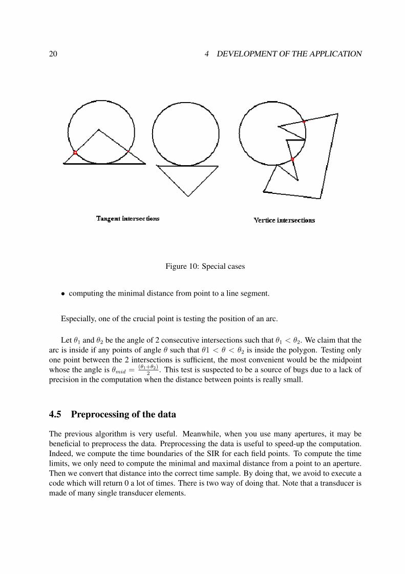
4.4.4 Special cases, tangents and corners

There are some special cases in the algorithm. One may have to deal with a tangent intersectionor a vertice intersection. The solution is to ignore the vertice intersections and the tangent in-tersection. One can notice that a circle contained in a square with tangent intersections at eachedge will be problematic. We avoid that case by the following method. We precompute beforethe minimal distance from the circle center to the polygon. If the center is inside the polygonand the radius of the circle is less or equal to dmin, it means that the whole circle is inside thepolygon. Thus the returned value will be 2π.

4.4.5 Geometric elements

The implementation of the algorithm relies on smaller algorithms of computational geometry.For example, we have implemented those algorithms:

• test wether a point lies on the left side of an directed line.

• test wether a point lies inside a polygon.

20 4 DEVELOPMENT OF THE APPLICATION

Figure 10: Special cases

• computing the minimal distance from point to a line segment.

Especially, one of the crucial point is testing the position of an arc.

Let θ1 and θ2 be the angle of 2 consecutive intersections such that θ1 < θ2. We claim that thearc is inside if any points of angle θ such that θ1 < θ < θ2 is inside the polygon. Testing onlyone point between the 2 intersections is sufficient, the most convenient would be the midpointwhose the angle is θmid = (θ1+θ2)

2. This test is suspected to be a source of bugs due to a lack of

precision in the computation when the distance between points is really small.

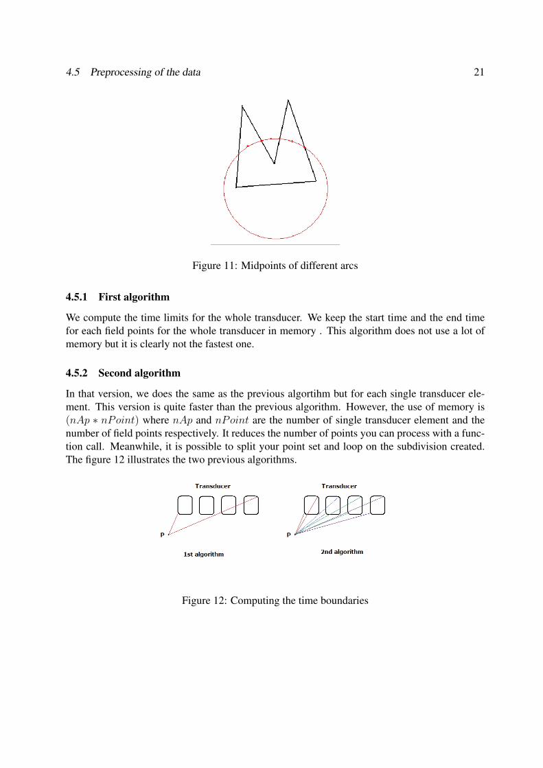
4.5 Preprocessing of the data

The previous algorithm is very useful. Meanwhile, when you use many apertures, it may bebeneficial to preprocess the data. Preprocessing the data is useful to speed-up the computation.Indeed, we compute the time boundaries of the SIR for each field points. To compute the timelimits, we only need to compute the minimal and maximal distance from a point to an aperture.Then we convert that distance into the correct time sample. By doing that, we avoid to execute acode which will return 0 a lot of times. There is two way of doing that. Note that a transducer ismade of many single transducer elements.

4.5 Preprocessing of the data 21

Figure 11: Midpoints of different arcs

4.5.1 First algorithm

We compute the time limits for the whole transducer. We keep the start time and the end timefor each field points for the whole transducer in memory . This algorithm does not use a lot ofmemory but it is clearly not the fastest one.

4.5.2 Second algorithm

In that version, we does the same as the previous algortihm but for each single transducer ele-ment. This version is quite faster than the previous algorithm. However, the use of memory is(nAp ∗ nPoint) where nAp and nPoint are the number of single transducer element and thenumber of field points respectively. It reduces the number of points you can process with a func-tion call. Meanwhile, it is possible to split your point set and loop on the subdivision created.The figure 12 illustrates the two previous algorithms.

Figure 12: Computing the time boundaries

22 5 RESULTS

5 ResultsThe machine I used was not CUDA capable so I connected to a CUDA capable machine withVNC viewer. As you can not debug GPU code, I debugged and tested the correctness of myCUDA code in emulator mode. It allows you to debug the code as it is emulated and runs like aC program.

5.1 Validation

In this version we present our results and discuss their validity compared to Field II and explainwhat are the new directions to take in order to achieve entirely the project.

5.1.1 Comparaison with Field II

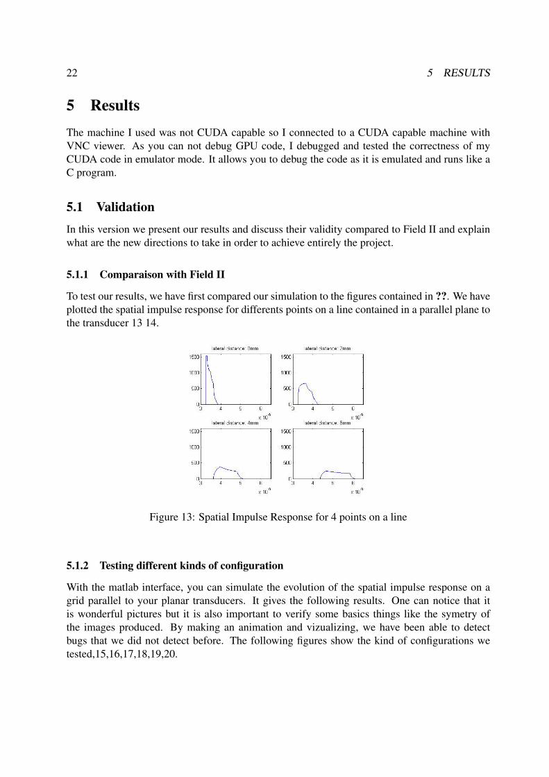
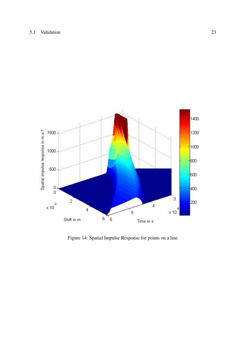
To test our results, we have first compared our simulation to the figures contained in ??. We haveplotted the spatial impulse response for differents points on a line contained in a parallel plane tothe transducer 13 14.

Figure 13: Spatial Impulse Response for 4 points on a line

5.1.2 Testing different kinds of configuration

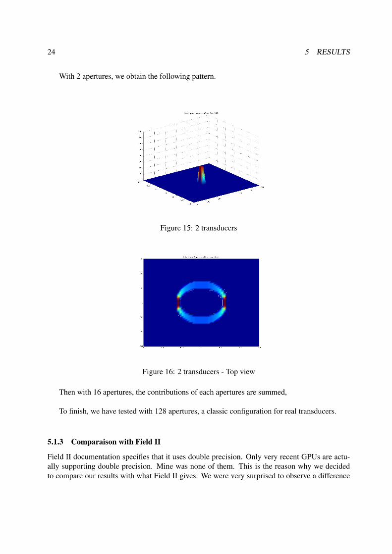
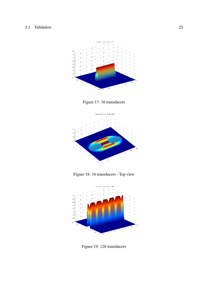
With the matlab interface, you can simulate the evolution of the spatial impulse response on agrid parallel to your planar transducers. It gives the following results. One can notice that itis wonderful pictures but it is also important to verify some basics things like the symetry ofthe images produced. By making an animation and vizualizing, we have been able to detectbugs that we did not detect before. The following figures show the kind of configurations wetested,15,16,17,18,19,20.

5.1 Validation 23

Figure 14: Spatial Impulse Response for points on a line

24 5 RESULTS

With 2 apertures, we obtain the following pattern.

Figure 15: 2 transducers

Figure 16: 2 transducers - Top view

Then with 16 apertures, the contributions of each apertures are summed,

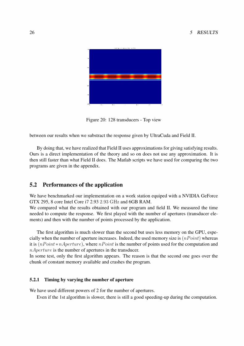
To finish, we have tested with 128 apertures, a classic configuration for real transducers.

5.1.3 Comparaison with Field II

Field II documentation specifies that it uses double precision. Only very recent GPUs are actu-ally supporting double precision. Mine was none of them. This is the reason why we decidedto compare our results with what Field II gives. We were very surprised to observe a difference

5.1 Validation 25

Figure 17: 16 transducers

Figure 18: 16 transducers - Top view

Figure 19: 128 transducers

26 5 RESULTS

Figure 20: 128 transducers - Top view

between our results when we substract the response given by UltraCuda and Field II.

By doing that, we have realized that Field II uses approximations for giving satisfying results.Ours is a direct implementation of the theory and so on does not use any approximation. It isthen still faster than what Field II does. The Matlab scripts we have used for comparing the twoprograms are given in the appendix.

5.2 Performances of the application

We have benchmarked our implementation on a work station equiped with a NVIDIA GeForceGTX 295, 8 core Intel Core i7 2.93 2.93 GHz and 6GB RAM.We compared what the results obtained with our program and field II. We measured the timeneeded to compute the response. We first played with the number of apertures (transducer ele-ments) and then with the number of points processed by the application.

The first algorithm is much slower than the second but uses less memory on the GPU, espe-cially when the number of aperture increases. Indeed, the used memory size is (nPoint) whereasit is (nPoint ∗nAperture), where nPoint is the number of points used for the computation andnAperture is the number of apertures in the transducer.In some test, only the first algorithm appears. The reason is that the second one goes over thechunk of constant memory available and crashes the program.

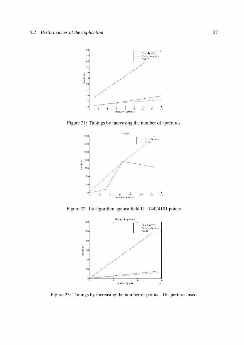
5.2.1 Timing by varying the number of aperture

We have used different powers of 2 for the number of apertures.Even if the 1st algorithm is slower, there is still a good speeding-up during the computation.

5.2 Performances of the application 27

Figure 21: Timings by increasing the number of apertures

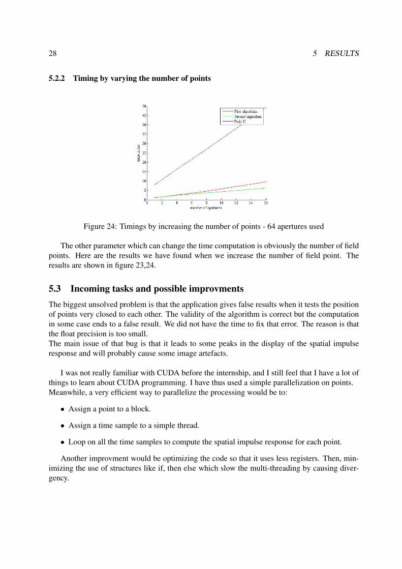
Figure 22: 1st algorithm against field II - 14424101 points

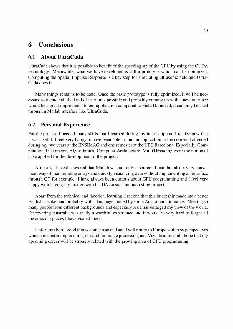
Figure 23: Timings by increasing the number of points - 16 apertures used

28 5 RESULTS

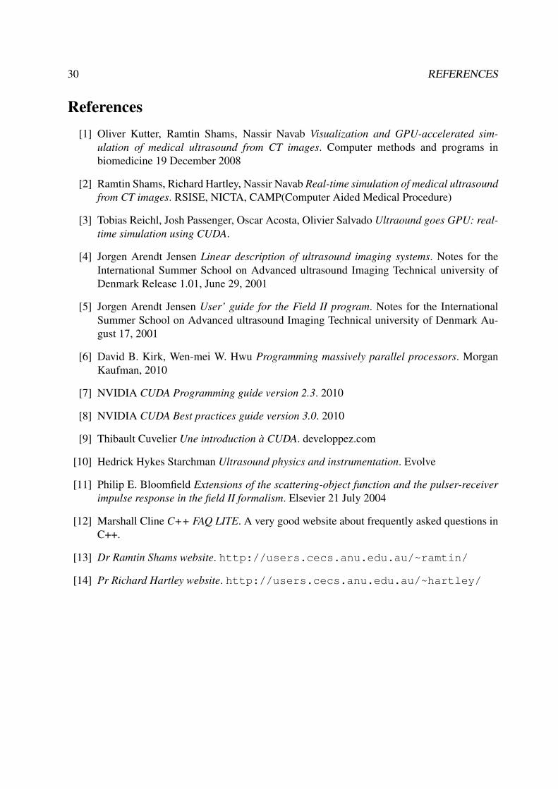
5.2.2 Timing by varying the number of points

Figure 24: Timings by increasing the number of points - 64 apertures used

The other parameter which can change the time computation is obviously the number of fieldpoints. Here are the results we have found when we increase the number of field point. Theresults are shown in figure 23,24.

5.3 Incoming tasks and possible improvmentsThe biggest unsolved problem is that the application gives false results when it tests the positionof points very closed to each other. The validity of the algorithm is correct but the computationin some case ends to a false result. We did not have the time to fix that error. The reason is thatthe float precision is too small.The main issue of that bug is that it leads to some peaks in the display of the spatial impulseresponse and will probably cause some image artefacts.

I was not really familiar with CUDA before the internship, and I still feel that I have a lot ofthings to learn about CUDA programming. I have thus used a simple parallelization on points.Meanwhile, a very efficient way to parallelize the processing would be to:

• Assign a point to a block.

• Assign a time sample to a simple thread.

• Loop on all the time samples to compute the spatial impulse response for each point.

Another improvment would be optimizing the code so that it uses less registers. Then, min-imizing the use of structures like if, then else which slow the multi-threading by causing diver-gency.

29

6 Conclusions

6.1 About UltraCudaUltraCuda shows that it is possible to benefit of the speeding-up of the GPU by using the CUDAtechnology. Meanwhile, what we have developed is still a prototype which can be optimized.Computing the Spatial Impulse Response is a key step for simulating ultrasonic field and Ultra-Cuda does it.

Many things remains to be done. Once the basic prototype is fully optimized, it will be nec-essary to include all the kind of apertures possible and probably coming up with a new interfacewould be a great improvment to our application compared to Field II. Indeed, it can only be usedthrough a Matlab interface like UltraCuda.

6.2 Personal ExperienceFor the project, I needed many skills that I learned during my internship and I realize now thatit was useful. I feel very happy to have been able to find an application to the courses I attendedduring my two years at the ENSIMAG and one semester at the UPC Barcelona. Especially, Com-putational Geometry, Algorithmics, Computer Architecture, MultiThreading were the notions Ihave applied for the development of the project.

After all, I have discovered that Matlab was not only a source of pain but also a very conve-nient way of manipulating arrays and quickly visualizing data without implementing an interfacethrough QT for exemple. I have always been curious about GPU programming and I feel veryhappy with having my first go with CUDA on such an interesting project.

Apart from the technical and theorical learning, I reckon that this internship made me a betterEnglish speaker and probably with a language tainted by some Australian idiomatics. Meeting somany people from different backgrounds and especially Asia has enlarged my view of the world.Discovering Australia was really a worthful experience and it would be very hard to forget allthe amazing places I have visited there.

Unfortunatly, all good things come to an end and I will return to Europe with new perspectiveswhich are continuing in doing research in Image processing and Vizualisation and I hope that myupcoming career will be strongly related with the growing area of GPU programming.

30 REFERENCES

References[1] Oliver Kutter, Ramtin Shams, Nassir Navab Visualization and GPU-accelerated sim-

ulation of medical ultrasound from CT images. Computer methods and programs inbiomedicine 19 December 2008

[2] Ramtin Shams, Richard Hartley, Nassir Navab Real-time simulation of medical ultrasoundfrom CT images. RSISE, NICTA, CAMP(Computer Aided Medical Procedure)

[3] Tobias Reichl, Josh Passenger, Oscar Acosta, Olivier Salvado Ultraound goes GPU: real-time simulation using CUDA.

[4] Jorgen Arendt Jensen Linear description of ultrasound imaging systems. Notes for theInternational Summer School on Advanced ultrasound Imaging Technical university ofDenmark Release 1.01, June 29, 2001

[5] Jorgen Arendt Jensen User’ guide for the Field II program. Notes for the InternationalSummer School on Advanced ultrasound Imaging Technical university of Denmark Au-gust 17, 2001

[6] David B. Kirk, Wen-mei W. Hwu Programming massively parallel processors. MorganKaufman, 2010

[7] NVIDIA CUDA Programming guide version 2.3. 2010

[8] NVIDIA CUDA Best practices guide version 3.0. 2010

[9] Thibault Cuvelier Une introduction à CUDA. developpez.com

[10] Hedrick Hykes Starchman Ultrasound physics and instrumentation. Evolve

[11] Philip E. Bloomfield Extensions of the scattering-object function and the pulser-receiverimpulse response in the field II formalism. Elsevier 21 July 2004

[12] Marshall Cline C++ FAQ LITE. A very good website about frequently asked questions inC++.

[13] Dr Ramtin Shams website. http://users.cecs.anu.edu.au/~ramtin/

[14] Pr Richard Hartley website. http://users.cecs.anu.edu.au/~hartley/

31

7 Appendix

7.1 Résumé du stageL’objectif du projet était de développer une simulation des champs ultrasoniques à partir d’unmodèle linéaire d’onde. La théorie est basée sur le formalisme de Tupholme-Stepanishen. Leprogramme de simulation Field II développé à l’Université Polytechnique du Danemark effectuecette simulation mais l’exécution du programme est longue car il utilise seulement le CPU demanière linéaire. Les principales tâches à effectuer étaient donc de créer et d’implémenter desalgorithmes adaptés au calculs effectués sur le GPU. Plus précisement, mon stage a consisté en:

• Se familiariser avec la physique des ultrasons et la programmation CUDA.

• Faire une première simulation via Matlab.

• Construire des algorithmes adaptés et optimisés pour la programmation GPU.

• Développer une application capable de simuler différents types de configuration et lesstructures de donnée correspondantes. L’application est appelée grâce à des commandesMatlab mais toutes les simulations sont éxécutées par le code C++/CUDA.

• Valider le programme et mesurer les temps d’éxécution.

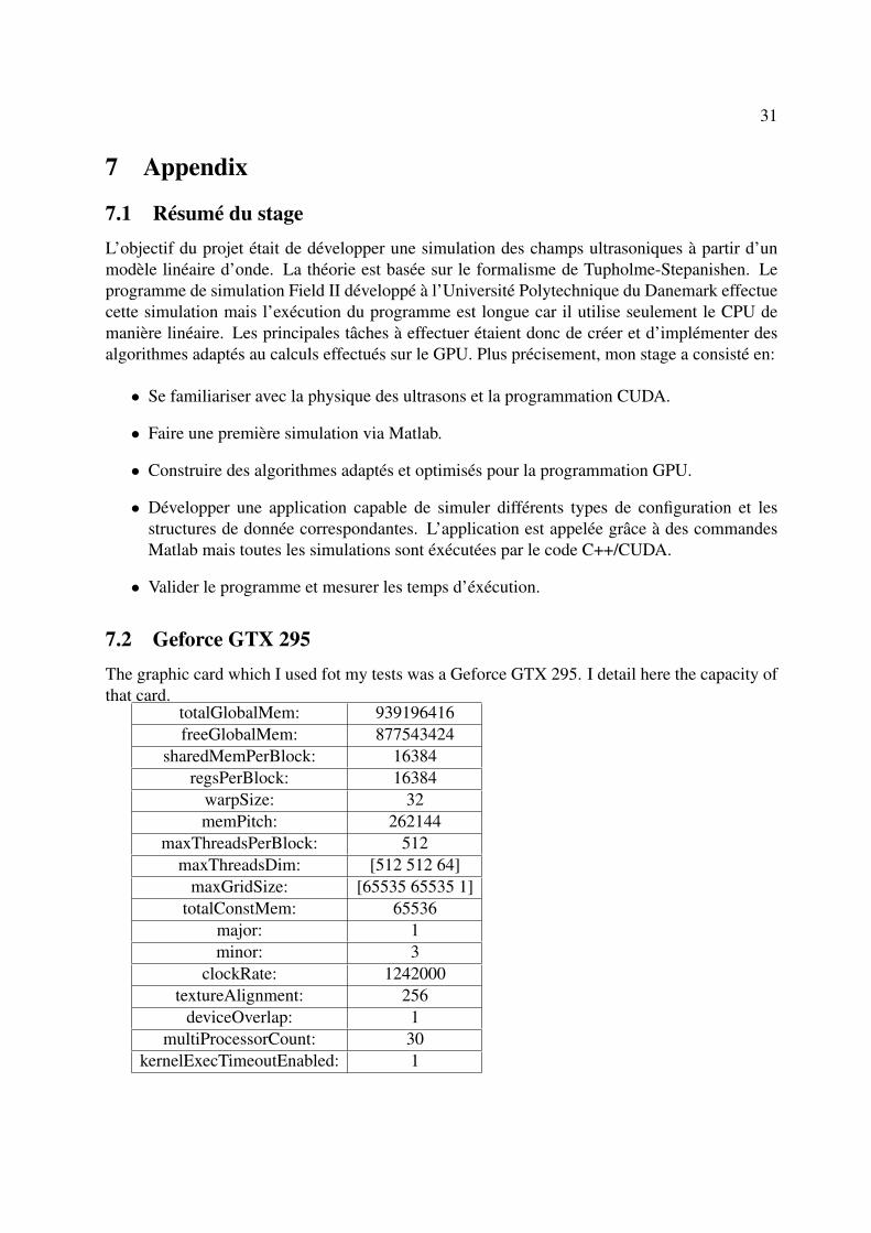
7.2 Geforce GTX 295The graphic card which I used fot my tests was a Geforce GTX 295. I detail here the capacity ofthat card.

totalGlobalMem: 939196416freeGlobalMem: 877543424

sharedMemPerBlock: 16384regsPerBlock: 16384

warpSize: 32memPitch: 262144

maxThreadsPerBlock: 512maxThreadsDim: [512 512 64]

maxGridSize: [65535 65535 1]totalConstMem: 65536

major: 1minor: 3

clockRate: 1242000textureAlignment: 256

deviceOverlap: 1multiProcessorCount: 30

kernelExecTimeoutEnabled: 1

32 7 APPENDIX

Typically, the gloabal memory is where I stored the preprocessed datas and the results. Itlimits so the number of processed points.The registers per blocks is the number of registers per shared processors. The more register youhave the best it is because the threads will not be queued. But not using all the registers willslower the execution also.The maximal dimensions of block and grid gives you what you can expect for a kernel configu-ration.

7.3 Some Matlab scripts

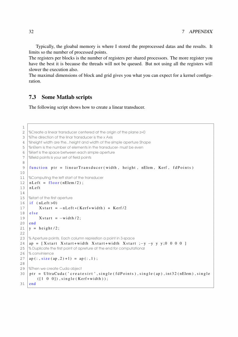
The following script shows how to create a linear transducer.

12 %Create a linear transducer centered at the origin of the plane z=03 %The direction of the linar transducer is the x Axis4 %height width are the...height and width of the simple aperture Shape5 %nElem is the number of elements in the transducer- must be even6 %Kerf is the space between each simple aperture7 %field points is your set of field points89 f u n c t i o n p t r = l i n e a r T r a n s d u c e r ( width , h e i g h t , nElem , Kerf , f d P o i n t s )

1011 %Computing the left start of the transducer12 n L e f t = f l o o r ( nElem / 2 ) ;13 n L e f t1415 %start of the first aperture16 i f ( nLef t >0)17 X s t a r t = −n L e f t ∗ ( Ker f + wid th ) + Kerf / 218 e l s e19 X s t a r t = −wid th / 2 ;20 end21 y = h e i g h t / 2 ;2223 % Aperture points. Each column represtion a point in 3-space24 ap = [ X s t a r t X s t a r t + wid th X s t a r t + wid th X s t a r t ;−y −y y y ; 0 0 0 0 ]25 % Duplicate the first point of apreture at the end for computational26 % convinience27 ap ( : , s i z e ( ap , 2 ) +1) = ap ( : , 1 ) ;2829 %Then we create Cuda object30 p t r = Ul t r aCuda ( ’ c r e a t e s i r t ’ , s i n g l e ( f d P o i n t s ) , s i n g l e ( ap ) , i n t 3 2 ( nElem ) , s i n g l e

( [ 1 0 0 ] ) , s i n g l e ( Ker f + wid th ) ) ;31 end

7.3 Some Matlab scripts 33

The following script generates an animation of the propagation of the wave on a parallelplane to the planar transducer.

1 %generate animation for the rectangular aperture2 g l o b a l c3 pause on45 % Initialise data6 % Resolution of the grid in meters7 r e s = 0 . 0 0 0 5 ;8 % Define the exents of the field plane9 x _ e x t =[−0.03 0 . 0 3 ] ;

10 y _ e x t =[−0.03 0 . 0 3 ] ;11 [X Y] = meshgr id ( x _ e x t ( 1 ) : r e s : x _ e x t ( 2 ) , y _ e x t ( 1 ) : r e s : y _ e x t ( 2 ) ) ;1213 % Plane depth where the SIR is computed14 z = 0 . 0 0 6 ;15 Z = z ∗ ones ( s i z e (X) ) ;1617 %making the grid18 f d P o i n t s = [X ( : ) ’ ;Y ( : ) ’ ; Z ( : ) ’ ] ;192021 % Aperture points. Each column represtion a point in 3-space22 % ap = [-0.0015 0.0015 0.0015 -0.0015 ;-0.0025 -0.0025 0.0025 0.0025 ;0 0 0 0 ];23 % Duplicate the first point of apreture at the end for computational24 % convinience25 % ap(:,size(ap,2)+1) = ap(:,1);2627 % Initializing the Cuda Object28 % ptr = UltraCuda(’creategridt’,single(X),single(Y),single(z),single(ap),int32(10),single([1 0

0]),single(0.0005));2930 %New version with centered aperture31 p t r = l i n e a r T r a n s d u c e r ( 1 / 1 0 0 0 , 5 / 1 0 0 0 , 10 , 1 / 1 0 0 0 , f d P o i n t s ) ;32 Ul t r aCuda ( ’ i n i t t ’ , p t r ) ;3334 % Time boundaries35 t = Ul t r aCuda ( ’ g e t t b t ’ , p t r )36 T = t ( 1 ) : t ( 2 ) ;3738 nFrames = s i z e ( T , 2 ) % a ver3940 v=view ( 3 ) ;41 f o r p =1: nFrames42 % Z=UltraCuda(’csirgridt’,single(T(p)),int32(size(X)),ptr);43 Z= Ul t r aCuda ( ’ c s i r t ’ , s i n g l e ( T ( p ) ) , p t r ) ;

34 7 APPENDIX

44 %loading image45 s u r f ( d ou b l e (X) , dou b l e (Y) , do ub l e ( r e s h a p e ( Z , s i z e (X, 1 ) , s i z e (X, 2 ) ) ) ) ;46 a x i s ( [ x_ext , y _ e x t 0 1 6 0 0 ] )47 % axis off;48 view ( v ) ;4950 s t r = s p r i n t f ( ’ S p a t i a l Impu l se Response on a P l a n e [ Frame %d/%d ] ’ ,T ( p )−T

( 1 ) +1 , numel ( T ) ) ;51 t i t l e ( s t r ) ;52 co lormap ( j e t )53 s h a d i n g f l a t ; s h a d i n g i n t e r p ; % Turn the grid off54 pause55 v=view ;56 end5758 Ul t r aCuda ( ’ c l e a n s i r t ’ , p t r ) ;59 c l e a r mex

I used the same kind of script for all the timing.

1 f u n c t i o n y = benchmark ( r e s )2 f i e l d _ i n i t ( ) ;3 nAp = [1 2 4 8 16 32 6 4 ] ;4 f o r i =1 : s i z e ( nAp , 2 )5 [m1 m2 m3 n f d p o i n t ] = t e s t T i m i n g ( 1 / 1 0 0 0 , 5 / 1 0 0 0 , nAp ( i ) , 0 . 0 5 / 1 0 0 0 , r e s ) ;6 y1 ( i ) =m1 ;7 y2 ( i ) =m2 ;8 y3 ( i ) =m3 ;9 end

10 y = n f d p o i n t ;111213 %do the plot14 ho ld on15 p l o t ( nAp , y1 , ’ r ’ , nAp , y2 , ’ g ’ , nAp , y3 , ’ b ’ ) ;16 x l a b e l ( ’ number o f a p e r t u r e s ’ ) ;17 y l a b e l ( ’ t ime i n ms ’ ) ;18 l e g e n d ( ’ F i r s t a l g o r i t h m ’ , ’ Second a l g o r i t h m ’ , ’ F i e l d I I ’ ) ;19 f i e l d _ e n d ( ) ;20 c l e a r mex ;

7.3 Some Matlab scripts 35

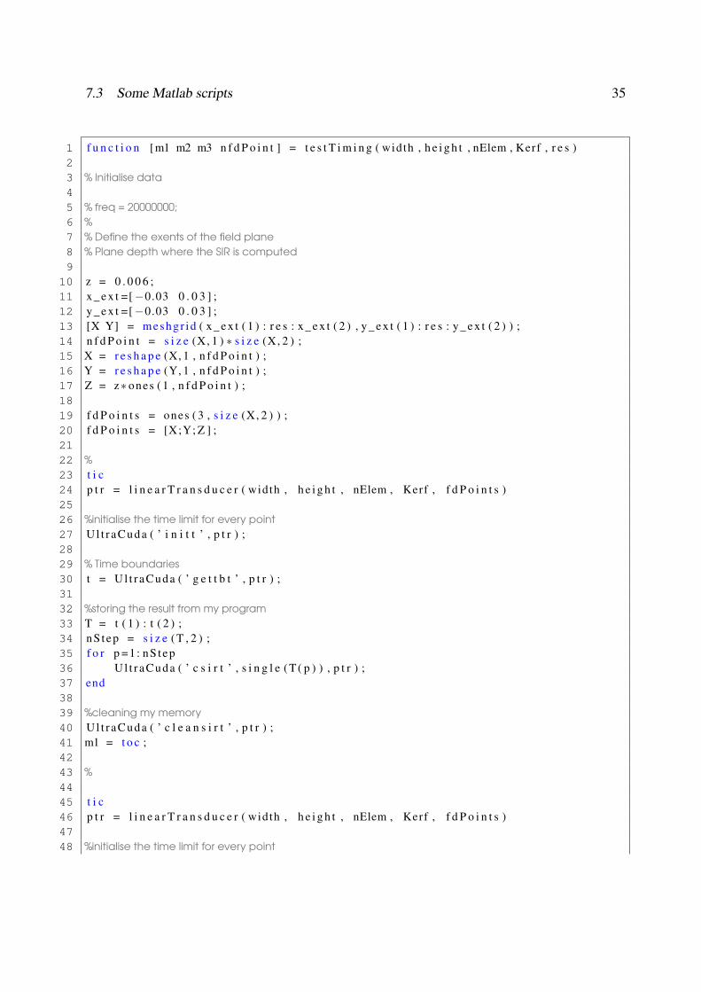
1 f u n c t i o n [m1 m2 m3 n f d P o i n t ] = t e s t T i m i n g ( width , h e i g h t , nElem , Kerf , r e s )23 % Initialise data45 % freq = 20000000;6 %7 % Define the exents of the field plane8 % Plane depth where the SIR is computed9

10 z = 0 . 0 0 6 ;11 x _ e x t =[−0.03 0 . 0 3 ] ;12 y _ e x t =[−0.03 0 . 0 3 ] ;13 [X Y] = meshgr id ( x _ e x t ( 1 ) : r e s : x _ e x t ( 2 ) , y _ e x t ( 1 ) : r e s : y _ e x t ( 2 ) ) ;14 n f d P o i n t = s i z e (X, 1 ) ∗ s i z e (X, 2 ) ;15 X = r e s h a p e (X, 1 , n f d P o i n t ) ;16 Y = r e s h a p e (Y, 1 , n f d P o i n t ) ;17 Z = z∗ ones ( 1 , n f d P o i n t ) ;1819 f d P o i n t s = ones ( 3 , s i z e (X, 2 ) ) ;20 f d P o i n t s = [X;Y; Z ] ;2122 %23 t i c24 p t r = l i n e a r T r a n s d u c e r ( width , h e i g h t , nElem , Kerf , f d P o i n t s )2526 %initialise the time limit for every point27 Ul t r aCuda ( ’ i n i t t ’ , p t r ) ;2829 % Time boundaries30 t = Ul t r aCuda ( ’ g e t t b t ’ , p t r ) ;3132 %storing the result from my program33 T = t ( 1 ) : t ( 2 ) ;34 nS tep = s i z e ( T , 2 ) ;35 f o r p =1: nS tep36 Ul t r aCuda ( ’ c s i r t ’ , s i n g l e ( T ( p ) ) , p t r ) ;37 end3839 %cleaning my memory40 Ul t r aCuda ( ’ c l e a n s i r t ’ , p t r ) ;41 m1 = t o c ;4243 %4445 t i c46 p t r = l i n e a r T r a n s d u c e r ( width , h e i g h t , nElem , Kerf , f d P o i n t s )4748 %initialise the time limit for every point

36 7 APPENDIX

49 Ul t r aCuda ( ’ i n i t t 2 ’ , p t r ) ;5051 % Time boundaries52 t = Ul t r aCuda ( ’ g e t t b t 2 ’ , p t r ) ;5354 %storing the result from my program55 T = t ( 1 ) : t ( 2 ) ;56 nS tep = s i z e ( T , 2 ) ;57 f o r p =1: nS tep58 Ul t r aCuda ( ’ c s i r t 2 ’ , s i n g l e ( T ( p ) ) , p t r ) ;59 end6061 %cleaning my memory62 Ul t r aCuda ( ’ c l e a n s i r t ’ , p t r ) ;63 m2 = t o c ;646566 %67 %doing the same for the field2 program68 %comparing with the field2 program69 t i c ;707172 %showing time73 s e t _ f i e l d ( ’ show_t imes ’ , 1 ) ;74 s e t _ f i e l d ( ’ c ’ , 1 5 4 8 ) ; %speed of sound in homogeneous medium75 s e t _ f i e l d ( ’ f s ’ ,20000000) ; %set the sampling frequency7677 f o c u s = [0 0 0 ] ;%No focus78 %79 %Converting the point into the field2 format80 f d P o i n t s = f d P o i n t s ’ ;81 Th = x d c _ l i n e a r _ a r r a y ( nElem , width , h e i g h t , Kerf , 3 , 5 , f o c u s ) ;8283 f o r i =1 : n f d P o i n t84 %computing the impulse response for point i85 [ h t s t a r t ] = c a l c _ h ( Th , f d P o i n t s ( i , : ) ) ;86 end8788899091 m3 = t o c ;9293 %clear mex filesx949596 end