ORIGINAL PAPER

Computational analysis of the SARS-CoV-2 and otherviruses based on the Kolmogorov’s complexityand Shannon’s information theories

J. A. Tenreiro Machado . Joao M. Rocha-Neves . Jose P. Andrade

Received: 26 April 2020 / Accepted: 14 June 2020 / Published online: 4 July 2020

� Springer Nature B.V. 2020

Abstract This paper tackles the information of 133

RNA viruses available in public databases under the

light of several mathematical and computational tools.

First, the formal concepts of distance metrics, Kol-

mogorov complexity and Shannon information are

recalled. Second, the computational tools available

presently for tackling and visualizing patterns embed-

ded in datasets, such as the hierarchical clustering and

the multidimensional scaling, are discussed. The

synergies of the common application of the mathe-

matical and computational resources are then used for

exploring the RNA data, cross-evaluating the normal-

ized compression distance, entropy and Jensen–

Shannon divergence, versus representations in two

and three dimensions. The results of these different

perspectives give extra light in what concerns the

relations between the distinct RNA viruses.

Keywords COVID-19 � Kolmogorov complexity

theory � Shannon information theory � Hierarchical

clustering � Multidimensional scaling

1 Introduction

In December 2019, a mysterious pneumonia with

unknown etiology was reported in the city of Wuhan,

Province of Hubei, China [1]. The International

Committee on Taxonomy of Virus (ICTV) named

the virus as severe acute respiratory syndrome coro-

navirus 2 (SARS-CoV-2) [2]. Globally, to the 30th of

July 2020, according to the World Health Organiza-

tion Coronavirus Disease 2019 (COVID-19) Situation

Report, 10,185, 374 confirmed cases of COVID-19 are

reported, resulting in 503,862 deaths.

The scientific community reacted as never before,

and many researchers focused on this urgent topic

[3–10]. The mathematical and computer science

communities are also studying this challenging prob-

lem, and we testimony the recent emergence of new

models and algorithmic approaches. This common

multidisciplinary research will allow the human kind

J. A. T. Machado (&)

Department of Electrical Engineering, Institute of

Engineering, Polytechnic of Porto, Rua Dr. Antonio

Bernardino de Almeida, 431, 4249-015 Porto, Portugal

e-mail: jtm@isep.ipp.pt

J. M. Rocha-Neves � J. P. Andrade

Department of Biomedicine – Unity of Anatomy, Faculty

of Medicine of University of Porto, Porto, Portugal

e-mail: joaorochaneves@hotmail.com

J. P. Andrade

e-mail: jandrade@med.up.pt

J. M. Rocha-Neves

Department of Physiology and Surgery, Faculty of

Medicine of University of Porto, Porto, Portugal

J. P. Andrade

Center for Health Technology and Services Research

(CINTESIS), Porto, Portugal

123

Nonlinear Dyn (2020) 101:1731–1750

https://doi.org/10.1007/s11071-020-05771-8(0123456789().,-volV)( 0123456789().,-volV)

to implement a robust and fast response to a problem

that is causing a severe global socioeconomic disrup-

tion, and most probably will lead to the largest global

recession since the Great Depression.

The present paper follows this trend by studying the

genetic information by means of mathematical and

computational tools. The starting point is the infor-

mation encoded in the ribonucleic acid (RNA), a

polymeric molecule essential in various biological

roles.

The evolutionary origin and divergence of eucary-

otes is mostly recoverable from their genetic relation-

ships. The phylogeny of core genes, such as those for

ribosomal proteins, provides a reasonable representa-

tion of many billions of years [11]. Unfortunately, the

diversity of viruses prevents such a reconstruction of

virus evolutionary histories as they lack any equiva-

lent set of universally conserved genes on which to

construct a phylogeny. Viral diversity is far greater

than that of other organisms, with significant differ-

ences in their genetic material, RNA or deoxyribonu-

cleic acid (DNA), and configurations (double or single

stranded), as well as the orientation of their encoded

gene. The smallest virus genomes [12] contain over

2,500 genes [13]. The RNA is a nucleic acid that is

essential to all forms of life, and it is found in nature

generally as single-stranded (ss) rather than a paired

double-stranded (ds) like DNA. In DNA, there are four

bases: adenine (A) complementary to thymine (T) and

cytosine (C) complementary to guanine (G). In the

RNA, uracil (U) is used instead of thymine.

Like DNA, RNA can carry genetic information. An

RNA virus is a virus that has RNA as its genetic

material encoding a number of proteins. This nucleic

acid is usually single-stranded RNA (ssRNA), but

there are double-stranded RNA (dsRNA) viruses.

These viruses exploit the presence of RNA-dependent

RNA polymerases in eucaryotes cells for replication

of their genomes. Many human diseases are caused by

such RNA viruses such as influenza, severe acute

respiratory syndrome (SARS), COVID-19, Ebola

disease virus, chikungunya, Zika virus, influenza B

and Lassa virus [14].

The RNA is usually sequenced indirectly by

copying it into complementary DNA (cDNA), which

is often amplified and subsequently analyzed using a

variety of DNA sequencing methods. Therefore, the

genomic sequences of the RNA viruses are published

presenting the four bases, namely adenine (A),

cytosine (C), guanine (G) and thymine (T).

This genetic information is analyzed by means of

the Kolmogorov’s complexity and Shannon’s infor-

mation theories. In the first case, the so-called

normalized information distance (NID) is adopted. In

the second, a statistical approach is considered, by

constructing histograms for the relative frequency of

three consecutive bases (triplets). The histograms are

interpreted under the light of entropy, cumulative

residual entropy and Jensen–Shannon divergence. The

results obtained for each theory, that is, the values

assessing the virus genetic code under the light of the

Kolmogorov’s complexity and the Shannon’s infor-

mation, are further processed by means of advanced

computational representation techniques. The final

visualization is obtained using the hierarchical clus-

tering (HC) [15–20] and multidimensional scaling

(MDS) techniques [21–27]. Three alternative repre-

sentations, namely dendrograms, hierarchical trees

and three-dimensional loci, are considered.

According to the ICTV, human coronavirus

belongs to the Betacoronavirus genus, a member of

the Coronaviridae family, categorized in the order

Nidovirales [28]. It has been categorized into several

genera, based on phylogenetic analyses and antigenic

criteria, namely: (i) Alphacoronavirus, responsible for

gastrointestinal disorders in humans, dogs, pigs and

cats; (ii) Betacoronavirus, including the bat coron-

avirus, the human severe acute respiratory syndrome

(SARS) virus, the Middle Eastern respiratory syn-

drome (MERS) virus and now the SARS-CoV-2; (iii)

Gammacoronavirus, which infects avian species; and

iv) Deltacoronavirus [2, 29].

Four coronaviruses broadly distributed among

humans (229E, OC43, NL63 and, HKU1) frequently

cause only common cold symptoms [2, 12]. The two

other strains of coronaviruses are linked with deadly

diseases and zoonotic in origin, i.e., the SARS-CoV

and MERS-CoV [30]. In 2002–2003, there was an

outbreak of SARS beginning in Guangdong Province

in China and affecting 27 countries subsequently [31].

It was considered the first pandemic event of the

twenty-first century, due to the SARS-CoV infecting

8098 individuals with 774 deaths [31]. In 2012, in the

Middle East, MERS-CoV caused a severe respiratory

disease that affected 2494 individuals and 858 deaths

[2]. In both epidemics, bats were the original host of

these two coronaviruses [2].

123

1732 J. A. T. Machado et al.

Coronaviruses contain a positive-sense, single-

stranded RNA genome. The genome size for coron-

aviruses ranges from 26.4 to 31.7 kilobases, and it is

one of the largest among RNA viruses.

The rapid spread of SARS-CoV-2 raises intriguing

questions such as whether its evolution is driven by

mutations, recombination or genetic variation [32].

This information is now being applied to the devel-

opment of diagnostic tools, effective antiviral thera-

pies and in the understanding of viral diseases.

Although numerous studies have been done from the

biological and medical perspective, to help further

understand SARS-CoV-2 and trace its origin, this

paper reports the use of multidimensional scale

techniques for the finding of the similarities and the

relationships among COVID-19 strains themselves

and between other described viruses.

For that, we have collected a set of 37 complete

genome sequences of SARS-CoV-2 virus obtained in

several countries from patients with COVID-19. To

help verify whether it is possible to trace the original

or intermediate host of SARS-CoV-2, we obtained the

genomic sequences of SARS-CoV-2 virus in other

hosts, including bats (16 genomic sequences), pan-

golins (8 genomic sequences) and environment (mar-

ket of Wuhan) [13]. We have also collected 23

genomic sequences of the coronavirus that cause mild

symptoms related to common cold in man (229E,

OC43, NL63 and, HKU1). The genomic sequences of

SARS-CoV (10 genomic sequences) and a MERS-

CoV (13 genomic sequences) were also gathered. For

comparison and control, we also obtained sequences

of other deadly pathogenic RNA viruses such as Lassa

(6 genomic sequences), Ebola (6 genomic sequences),

dengue (7 genomic sequences), chikungunya (1

genomic sequence) and influenza B (2 genomic

sequences).

The diagram of Fig. 1 summarizes the main

historical flow of coronavirus in what concerns the

twenty-first-century epidemics.

To the authors’ best knowledge, this paper analyzes

for the first time a large number of viruses associated

with the combination of several distinct mathematical

and computational tools. In short, we have the cross-

comparison of:

– The genomic sequences of 133 viruses.

– The data treatment by means of Kolmogorov’s

complexity and Shannon’s information theories,

using normalized compression distance, entropy,

cumulative residual entropy and Jensen–Shannon

divergence.

– Two clustering computational techniques, namely

the hierarchical clustering and multidimensional

scaling.

– The visualization of the results by means of

dendrograms, trees and point loci.

The results indicate clearly the superior performance

of the approaches based on the Kolmogorov’s com-

plexity measure and the MDS three-dimensional

visualization. Moreover, the characteristics of the

coronaviruses within the large set of tested cases are

highlighted. We conclude that:

– The association between the Kolmogorov perspec-

tive and the three-dimensional MDS representa-

tion leads to be the best results.

– The clusters are easily distinguishable and we

observe the relation between the new SARS-CoV-

2 virus and some CoV found in bats and in the

pangolin.

Fig. 1 Coronavirus related

to twenty-first-century

epidemics. ICST: The

International Committee on

Taxonomy of Virus—

Coronavirus Study Group,

WHO: World Health

Organization

123

Computational analysis of SARS-CoV-2 genome 1733

Bearing these ideas in mind, the paper is organized as

follows. Section 2 introduces the mathematical and

computational tools adopted in the follow-up. Sec-

tion 3 analyzes the data by means of the complexity

and information theories accompanied by the HC and

MDS computational visualization resources. Finally,

Sect. 4 summarizes the main conclusions.

2 Fundamental tools

2.1 Distance metrics

Evaluating the similarity degree between several

objects, each having a number of features requires

the definition of a distance. The calculation of a

function d of two objects xA and xB can be interpreted

as a distance if dðxA; xBÞ� 0 and satisfies the following

axioms [33]:

identity : dðxA; xBÞ ¼ 0 if xA ¼ xB

symmetry : dðxA; xBÞ ¼ dðxB; xAÞ

triangle inequality : dðxA; xBÞ� dðxA; xCÞ

þ dðxC; xAÞ:

ð1Þ

We find in the literature a variety of different

functions that can tackle datasets and shed light to

distinct characteristics [34]. For a set of numerical

vectors x1; . . .; xNð ÞT2 Rn, the Minkowski norm

Ln :PN

k¼1 xkj jn� �1

n, and in particular the Manhattan

and Euclidean cases, L1 and L2 for n ¼ 1 and n ¼ 2,

are often used [35]. In the case of DNA analysis, these

norms support different algorithms [36–38] that allow

the comparison of data sequences. We can also

mention metrics such as the Chi-square [39], Ham-

ming [40] and edit [41] distances. Nonetheless, the

selection of the optimal distances for a specific

application poses relevant challenges [42–45]. In fact,

the adoption of a given metric often depends on the

user experience that performs several numerical

experiments before selecting one or more distances.

Due to these issues, assessing the similarity of several

objects is not a straightforward process and we can

adopt both non-probabilistic and probabilistic infor-

mation measures to obtain distinct perspectives

between object similarities.

2.2 Kolmogorov complexity theory

The Kolmogorov complexity, or algorithmic entropy,

addresses the information measurement without rely-

ing on probabilistic assumptions. The information

measurement focuses an individual finite object

described by a string and takes into consideration that

‘regular’ strings are compressible [46]. The Kol-

mogorov complexity of a string x, denoted as K(x), can

be defined as the length of the shortest binary program

that, given an empty string w at its input, can compute

x on its output in a universal computer, and then halts.

Therefore, K(x) can be interpreted as the length of the

ultimate compressed version of x.

The information distance of two strings (or files)

fxA; xBg 2 R, where R denotes the space of the

objects, can also be computed by means of the

conditional Kolmogorov complexity KðxAjxBÞ[47, 48]. This concept can be read as the length of

the shortest program to obtain xA, if xB is provided for

input. In heuristic terms, if the two strings are

more/less similar, then the calculation is less/more

difficult and, consequently, the size of the program is

smaller/larger. Therefore, the following inequality

always holds

KðxAjxBÞ�KðxAÞ: ð2Þ

Under the light of these concepts, the universal

distance metric [47] denoted as normalized informa-

tion distance (NID):

NIDðxA; xBÞ

¼ maxfKðxAjxBÞ;KðxBjxAÞgmaxfKðxAÞ;KðxBÞg

; fxA; xBg 2 R;

ð3Þ

was proposed.

From equation (2), we have that the NID may take

values in the range [0, 1]. Moreover, we have

NIDðxA; xAÞ � 0 and NIDðxA;wÞ � 1, where w is an

empty object that has no similarity to xA. It is shown

[47] that the NID is a distance because it satisfies the

axioms defined in (1), up to some additive precision,

but is non-computable [47]. In spite of this limitation,

the NID gives the basis for the so-called normalized

compression distance (NCD), which is a com-

putable distance [45]. The computability comes with

the cost of using a good approximation of the

Kolmogorov complexity by a standard compressor

123

1734 J. A. T. Machado et al.

Cð�Þ (interested readers for the discussion between the

equivalence of the NID and the NCD can find further

details in [33]).

The NCD is given by:

NCDðxA; xBÞ ¼CðxAxBÞ � minfCðxAÞ;CðxBÞg

maxfCðxAÞ;CðxBÞg:

ð4Þ

The NCD has values in the range

0\NCDðx; yÞ\1 þ �, assessing the distance between

the files xA and xB. The parameter �[ 0 reflects

‘imperfections’ in the compression algorithm. The

values of CðxAÞ and CðxBÞ are the sizes of each of the

compressed files xA and xB, respectively, and CðxAxBÞis the compressed size of the two concatenated files

considered by the compressor as a single file.

Let us consider, for example, that CðxBÞ�CðxAÞ.Expression (4) says that the distance NCDðxA; xBÞassesses the improvement due to compressing xB using

data from the previously compressed xA and com-

pressing xB from scratch, expressed as the ratio

between their compressed sizes.

Obviously, the approximation of the NID by means

of theNCD poses operational obstacles. Due to the non-

computability of the Kolmogorov complexity, we

cannot predict how close is the NCD to the real value

of the NID, and the approximation may yield arithmetic

problems, particularly in the case of small strings where

numerical indeterminate forms may arise [33, 49].

Moreover, the compressor (as an approximation of the

Kolmogorov complexity) must be ‘normal’ in the sense

that given the object xAxA the compressor C should

produce an object with almost to an identical size to

the compressed version of xA. This is a limitation for

the universality of the NCD since in specific applica-

tions the best performing loss-less algorithms (e.g.,

JBIG, JPEG2000 and JPEG-LS in image compression)

do not satisfy such propriety [50]. Nevertheless, key

results were already obtained using the NCD in image

distinguishability [51], image OCR [52], malware

recognition [53] and genomic analysis [54, 55].

2.3 Shannon information theory

Information theory [56] has been applied in a variety

of scientific areas. The most fundamental piece of the

theory is the information content I of a given event xihaving probability of occurrence P X ¼ xið Þ:

I X ¼ xið Þ ¼ � ln P X ¼ xið Þð Þ; ð5Þ

where X is a discrete random variable.

The expected value of the information, the so-

called Shannon entropy [57, 58], is given by:

H Xð Þ ¼E � ln Xð Þð Þ¼�

X

i

P X ¼ xið Þ ln P X ¼ xið Þð Þ; ð6Þ

where E �ð Þ denotes the expected value operator.

Expression (6) obeys the four Khinchin axioms

[59, 60]. Several generalizations of Shannon entropy

have been proposed, relaxing some of those axioms,

and we can mention the Renyi, Tsallis and generalized

entropy [61–63], just to name a few.

A recent and interesting concept is the cumulative

residual entropies e given by [64, 65]:

e Xð Þ ¼ �X

i

P X[ xið Þ log P X[ xið Þð Þ: ð7Þ

Within the scope of information theory, we can

formulate also the concept of distance discussed in

Sect. 2.1. The Kullback–Leibler divergence between

the probability distributions X1 and X2 is defined as

[34, 66–69]:

DKL X1 k X2ð Þ ¼X

i

P X1 ¼ xið Þ lnP X1 ¼ xið ÞP X2 ¼ xið Þ

� �

:

ð8Þ

From this, we obtain the Jensen–Shannon divergence,

JSD X1 k X2ð Þ, or distance, given by:

JSD X1 k X2ð Þ

¼ 1

2DKL X1 k X12ð Þ þ DKL X2 k X12ð Þ½ �;

ð9Þ

where X12 ¼ 12X1 þ X2ð Þ.

Alternatively, the JSD X1 k X2ð Þ can be calculated

as:

JSD X1 k X2ð Þ ¼ 1

2

X

i

P X1 ¼ xið Þ ln P X1 ¼ xið Þð Þ

þ 1

2

X

i

P X2 ¼ xið Þ ln P X2 ¼ xið Þð Þ

�X

i

P X12 ¼ xið Þ ln P X12 ¼ xið Þð Þ:

ð10Þ

123

Computational analysis of SARS-CoV-2 genome 1735

2.4 Hierarchical clustering, multidimensional

scaling and visualization

The HC is a computational technique that assesses a

group of N objects Xi, i ¼ 1; � � � ;N, in a q-dimensional

space, and tries to rearrange them in a visual structure

with objects Yi highlighting the main similarities

between them in the sense of some predefined metric

[70].

Let us consider N objects defined in a q-dimen-

sional real-valued space and a distance (or dissimilar-

ity) measure dij between pairs of objects. The first step

is to calculate a N � N-dimensional matrix, D ¼ ½dij�,where dij 2 Rþ for i 6¼ j and dii ¼ 0, ði; jÞ ¼ 1; � � � ;N,

stands for the object to object distances [71]. The HC

uses the input information in matrix D and produces a

graphical representation consisting in a dendrogram or

a hierarchical tree.

The so-called agglomerative or divisive clustering

iterative techniques are usually adopted for processing

the information. In the first approach, each object

starts in its own cluster and the computational

iterations merge the most similar items until having

just one cluster. In the second, all objects start their

own cluster and the computational iterations separate

items, until each object has his own cluster. For both

approaches, the numerical iterations follow a linkage

criterion, based on the distances between pairs, for

quantifying the dissimilarity between clusters. The

maximum, minimum and average linkages are possi-

ble criteria. The distance d xA; xBð Þ between two

objects xA 2 A and xB 2 B can be assessed by means

of several metrics such as the average linkage given by

[72]:

dav A;Bð Þ ¼ 1

Ak k Bk kX

xA2A;xB2Bd xA; xBð Þ: ð11Þ

The clustering quality can be assessed by means of the

cophenetic correlation [73]:

c ¼P

i\j xði; jÞ � �xð Þ yði; jÞ � �yð ÞffiffiffiffiffiffiffiffiffiffiffiffiffiffiffiffiffiffiffiffiffiffiffiffiffiffiffiffiffiffiffiffiffiffiffiffiffiffiffiffiffiffiffiffiffiffiffiffiffiffiffiffiffiffiffiffiffiffiffiffiffiffiffiffiffiffiffiffiffiffiffiffiffiffiffiffiffiffiffiP

i\j xði; jÞ � �xð Þ2h i P

i\j yði; jÞ � �yð Þ2h ir ;

ð12Þ

where x(i, j) and y(i, j) stand for the distances between

the pairs Xi and Xj, in the initial measurements, and Yi

and Yj, in the HC chart, respectively, and �x denotes the

average of x.

Values of c close to 1 (to 0) indicate a good (weak)

cluster representation of the original data. In

MATLAB, c is computed by means of the command

cophenet.

In this paper, we adopt the agglomerative clustering

and the average linkage [74, 75] for tackling the matrix

of distances based on the JSD metric (10).

The MDS is also a computational technique for

clustering and visualizing multidimensional data [76].

Similarly to what was said for the HC, the input of the

MDS is the matrix D ¼ ½dij�, ði; jÞ ¼ 1; � � � ;N. The

MDS is to adopt points for representing the objects in a

d-dimensional space, with d\q, that try to reproduce

the original distances, dij. The MDS performs a series

of numerical iterations rearranging the points in order

to optimize a given cost function called stress S. We

have, for example, the residual sum of squares and the

Sammon criteria:

S ¼X

i\j

/ij � dij� �2

" #12

; ð13aÞ

S ¼P

i\j /ij � dij� �2

Pi\j /

2ij

" #12

: ð13bÞ

The resulting MDS points have coordinates that

produce a symmetric matrix U ¼ ½/ij� of distances that

approximate the original one D ¼ ½dij�. In MATLAB,

the commands cmdscale and Sammon can be

adopted for the classical MDS and the Sammon stress

criterion.

The interpretation of the MDS locus is based on the

patterns of points [77, 78]. Therefore, objects with

strong (weak) similarities are represented by fairly

close (distant) points. The MDS locus is interpreted on

the relative positions of the point coordinates. So, the

absolute position of the points or the shape of the

clusters has usually a special meaning, and we can

magnify, translate and rotate the locus for achieving a

good visualization. In the same line of reasoning, the

axes of the plot do not have units or physical meaning.

The quality of the produced MDS locus can be

evaluated using the stress plot and the Shepard

diagram. The stress plot shows S versus d and

decreases monotonically. Usually, low values of d

are adopted, and present computational resources

123

1736 J. A. T. Machado et al.

allow a direct three-dimensional representation, but

often some rotations and magnification are required to

achieve the best visual perspective. The Shepard

diagram plots /ij against dij for a given value of d, and

a narrow (large) scatter of points indicates a good

(weak) fit between the original and the reproduced

distances.

3 The dataset

The information of 133 publicly released genomic

sequences was collected in the Global Initiative on

Sharing Avian Influenza Data (GISAID) and the

GenBank of the National Center for Biotechnology

Information (NCBI) databases (https://www.gisaid.

org/, https://www.ncbi.nlm.nih.gov/genbank). The

information regarding the sequences and serial num-

bers is given in Table of ‘‘Appendix.’’

The mathematical tools of Kolmogorov and Shan-

non theories are used to compare and extract relation-

ships among the data and to identify viral genomic

patterns. The viral genomes are analyzed from the

perspective of dynamical systems using HC and MDS.

Dendrograms and trees are generated by HC algo-

rithms, and a three-dimensional visualization through

MDS visualization. Several clusters with medical and

epidemiological interest were visualized. The MDS

loci provide a key visualization of the relation of

SARS-CoV-2 with the other known coronavirus

affecting humans.

The several non-coronavirus pathogenic viruses

analyzed are very well delimited in several indepen-

dent and easily delineated clusters (Zika, Chikun-

gunya, Dengue, Lassa, Ebola, Influenza B).

The several types of coronaviruses that cause mild

disease (common flu) are very well separated from the

other coronavirus clusters. Interestingly, the types,

229E, HkU1, NL63 and OC43, form separated mini-

clusters within a big well-defined cluster

There are two well-defined CoV-19 or SARS-CoV

clusters. The two environmental SARS-CoV-2 were

aggregated with the human SARS-CoV-2. To differ-

entiate the human MERS-CoV, a zoom was made to

isolate it forming a separate cluster. The MERS-CoV

obtained from camels was included in this cluster.

SARS-CoV formed another independent and well-

segregated cluster. The CoV from bats and pangolin is

dispersed among these several clusters of coronavirus

forming sometimes clusters of few elements. Note that

the bat CoV RaTG13 is near to one of the SARS-CoV

clusters. This coronavirus is the closest known relative

of SARS-CoV-2 [79].

For processing the RNA information consisting of

ASCII files with the four nitrogenous bases, we

consider two approaches. The first one follows the

Kolmogorov complexity theory described in Sect. 2.2.

Therefore, we consider the compressors zlib and

bz2 (see https://www.zlib.net and https://sourceware.

org/bzip2/) followed by the NCD distance (4).

Nonetheless, the two algorithms give almost identical

results, and therefore, only the zlib is considered in

the follow-up.

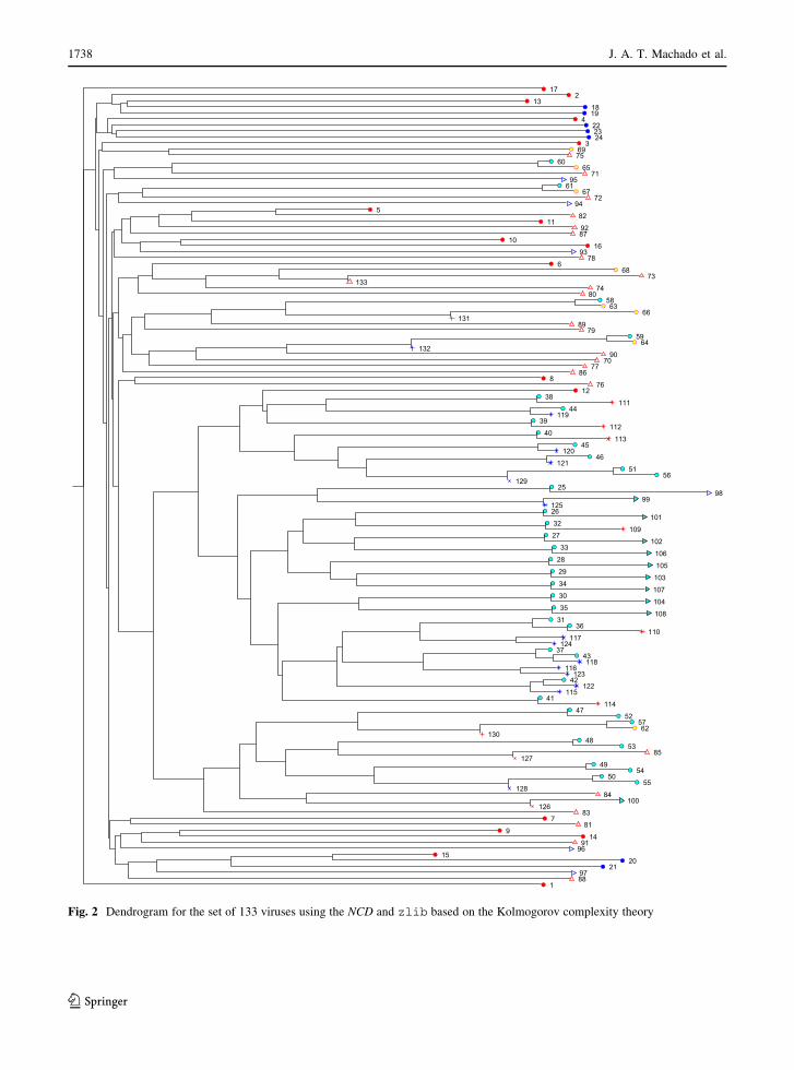
The application of the NCD produces a symmetrical

matrix D, 133 � 133 dimensional that is tackled and

visualized by means of a dendrogram and a HC tree

obtained by the program Phylip http://evolution.

genetics.washington.edu/phylip.html and MDS using

MATLAB https://www.mathworks.com/products/

matlab.html. The corresponding charts are repre-

sented in Figs. 2, 3 and 4.

It is known that the three-dimensional plots require

some rotation in the computer screen. Therefore,

Fig. 5 shows the MDS locus in a different perspective,

without point labels and the cluster of SARS-CoV-2

connected by a line.

The second approach follows the Shannon infor-

mation theory described in Sect. 2.3. Therefore, we

start by considering non-overlapping (codon or anti-

codon) triplets of bases and the histograms of relative

frequency for each virus. In a second phase, after

having the histogram for the complete set of virus, we

process them using entropy concepts. Before contin-

uing, we must clarify that we tested the adoption of n-

tuples, with n ¼ 1; 2; 3; 4, in the DNA information

analysis of a large set of superior species such as

mammals, where the genetic information is consider-

ably larger and the construction of histograms for large

values of n does not pose problems of statistical

significance (since the number of histograms bins

grows as 4n). It was observed that n ¼ 3 is a ‘good

value,’ since n ¼ 1 leads to poor results, n ¼ 2

improves things but is still insufficient, while n ¼ 4

gives almost identical results to n ¼ 3.

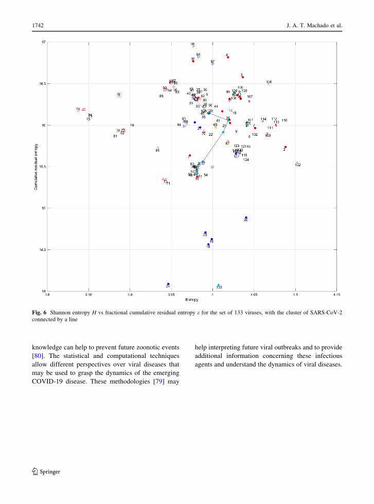
In a first experiment, we consider the Shannon

entropy H vs fractional cumulative residual entropy eas possible descriptors of the 133 histograms. Figure 6

123

Computational analysis of SARS-CoV-2 genome 1737

172

131819

4222324

36975

6065

7195

6167

7294

582

119287

1016

9378

668

73133

7480

5863

66131

8979

5964

13290

7077

868

7612

38111

44119

39112

40113

45120

46121

5156

12925

9899

12526

10132

10927

10233

10628

10529

10334

10730

10435

10831

36110

117124

3743118

11612342

122115

41114

4752

5762

13048

5385

12749

5450

55128

84100

12683

781

914

9196

1520

219788

1

Fig. 2 Dendrogram for the set of 133 viruses using the NCD and zlib based on the Kolmogorov complexity theory

123

1738 J. A. T. Machado et al.

shows the resulting two-dimensional plot, that is, the

Shannon entropy H vs the fractional cumulative

residual entropy e, for the set of 133 viruses. We

observe some separation between virus, but we have

some difficulties due to the high density of points in

some areas.

We now try the other computational techniques

introduced in Sect. 2. In the follow-up, we consider

identical input information, that is, the JDS and the

corresponding matrix D for the set of 133 viruses, and

we compare the distinct computational clustering and

visualization techniques.

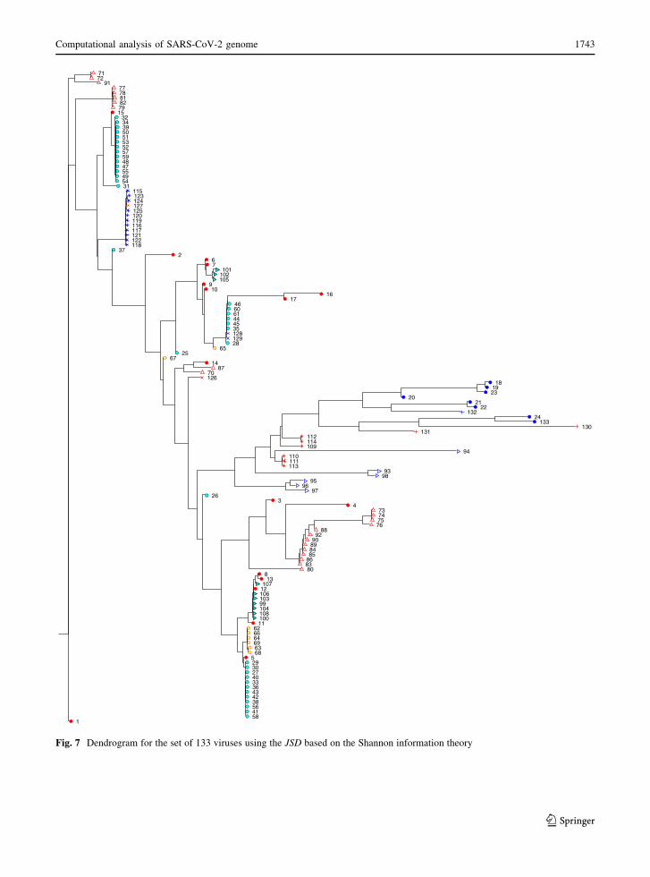
Figures 7, 8 and 9 show the dendrogram, the HC

tree and the three-dimensional MDS locus,

respectively. The dendrogram is the simplest repre-

sentation and it is straightforward to interpret. How-

ever, this technique does not take full advantage of the

space. The HC tree uses more efficiently the two-

dimensional space, but we now have more difficulties

in reading the most dense clusters. The three-dimen-

sional MDS takes advantage of the computational

representation, but requires some rotation/shift/mag-

nification in the computer screen.

Successive magnifications can be done and are

necessary to achieve a more distinct visualization.

Therefore, we can say that all representations have

their own pros and cons, although the three-dimen-

sional MDS is, a priori, the most efficient method.

172

13

1819422

2324

369

75

606571

95

616772

94

5

82

119287

1016

93

78

6

68

73133

7480

58

63

66 13189

79

5964 132

9070 77 86

8

76

1238

111

44119

39

112

40

113

45120

46

121

51

56

12925

98

99

12526 101

32

109

27102

33 106

28 105

29 103

34 107

30 104

35

108

31 36

110117 12437

43

11811612342 122115

41114

47 5257

62130

4853

85127

49

5450

55

128

84

100

12683

7

81

9

149196

15

2021

97881

Fig. 3 HC tree for the set of 133 viruses using the NCD and zlib based on the Kolmogorov complexity theory

123

Computational analysis of SARS-CoV-2 genome 1739

Since the three-dimensional plot requires some

rotation in the computer screen, Fig. 10 shows the

MDS locus in a different perspective, without point

labels and the cluster of SARS-CoV-2 connected by a

line.

The MDS 3D following the Kolmogorov method

isolated the several groups of virus in several extended

groups. The cluster of SARS-CoV-2 is very extended.

Note that the SARS-CoV-2 virus found in the market

of Wuhan is very near of the SARS-CoV-2 cluster.

The CoV found in the pangolin also forms a cluster

mixing with the upper part of the SARS-CoV-2

cluster. Bat CoV virus forms also a diffuse cluster

lacking some contiguity. The bat CoV Yunnan

RaTG13 is very near the SARS-CoV-2 cluster. There

is a big cluster formed by the different CoV that causes

a mild respiratory disease (common cool).

Other pathogenic RNA virus clusters, i.e., Lassa

virus, Zika, influenza B and Ebola, can be easily

separated from the CoV clusters. However, with this

methodology, the cluster formed by the dengue virus is

not very far, in some views, from a part of the cluster

formed by the CoV that causes mild respiratory

disease.

The SARS CoV virus forms another independent

cluster. MERS-CoV from humans forms another

extended cluster and in the vicinity of the CoV virus

from camel.

Fig. 4 MDS three-dimensional locus for the set of 133 viruses using the NCD and zlib based on the Kolmogorov complexity theory

with the cluster of SARS-CoV-2 connected by a line

123

1740 J. A. T. Machado et al.

4 Conclusions

This paper explored the information of 133 RNA

viruses available in public databases. For that purpose,

several mathematical and computational tools were

applied. On the one hand, the concepts of distance and

the theories developed by Kolmogorov and Shannon

for assessing complexity and information were

recalled. The first involved the normalized compres-

sion distance and the zlib compressor for the DNA.

The second understood the use of histograms of

triplets of bases and their assessment through entropy,

cumulative residual entropy and Jensen–Shannon

divergence. On the other hand, the advantages of

hierarchical clustering and multidimensional scaling

algorithmic techniques were also discussed. Repre-

sentations in two and three dimensions, namely by

dendrograms and trees, and loci of points or points and

lines, respectively, were compared. The results

revealed their pros and cons for the specific applica-

tion of the set of viruses under comparison.

The MDS 3D in the Kolmogorov perspective leads

to be the best visualization method. We have not only

the clusters easily distinguishable, but we find also the

relation between the new SARS-CoV-2 virus and

some CoV found in bats (the primary host of the virus)

and in the pangolin, the likely intermediate host. The

SARS-CoV-2 found in the environment, namely the

Market of Wuhan where the epidemic probably

started, is indistinguishable from the SARS-CoV-2

found in humans.

This type of methodology may help to study how an

animal virus jumped the boundaries of species to

infect humans, and pinpoint its origin, as this

Fig. 5 MDS three-dimensional locus for the set of 133 viruses using the NCD and zlib based on the Kolmogorov complexity theory,

without point labels and the cluster of SARS-CoV-2 connected by a line

123

Computational analysis of SARS-CoV-2 genome 1741

knowledge can help to prevent future zoonotic events

[80]. The statistical and computational techniques

allow different perspectives over viral diseases that

may be used to grasp the dynamics of the emerging

COVID-19 disease. These methodologies [79] may

help interpreting future viral outbreaks and to provide

additional information concerning these infectious

agents and understand the dynamics of viral diseases.

Fig. 6 Shannon entropy H vs fractional cumulative residual entropy e for the set of 133 viruses, with the cluster of SARS-CoV-2

connected by a line

123

1742 J. A. T. Machado et al.

7172

91777881827915323439505153525759484755495431

115123124127125120119116117121122118

372

67

101102105

910

1617

46606144453512812928

6525

6714

8770126

181923

202122

13224133

130131

112114109

94110111113

9398

9596

9726

34

73747576

8892

90898485868380

813

107121061039910410810011

626664696368

5293027403336434238564158

1

Fig. 7 Dendrogram for the set of 133 viruses using the JSD based on the Shannon information theory

123

Computational analysis of SARS-CoV-2 genome 1743

Fig. 8 HC tree for the set of 133 viruses using the JSD based on the Shannon information theory

123

1744 J. A. T. Machado et al.

Fig. 9 MDS three-dimensional locus for the set of 133 viruses using the JSD based on the Shannon information theory, with the cluster

of SARS-CoV-2 connected by a line

123

Computational analysis of SARS-CoV-2 genome 1745

Acknowledgements The authors thank all those who have

contributed and shared sequences to the GISAID database

(https://www.gisaid.org/). The authors also thank those who

have contributed to the GenBank of the National Center for

Biotechnology Information (NCBI) databases (https://www.

ncbi.nlm.nih.gov/genbank). The authors also thank Romulo

Antao for the help in handling the information with the com-

pressors zlib and bz2.

Compliance with ethical standards

Conflict of interest The authors declare that they have no

conflict of interest.

Fig. 10 MDS three-dimensional locus for the set of 133 viruses using the JSD based on the Shannon information theory, without point

labels and the cluster of SARS-CoV-2 connected by a line

123

1746 J. A. T. Machado et al.

Appendix

123

Computational analysis of SARS-CoV-2 genome 1747

References

1. Zhu, N., Zhang, D., Wang, W., Li, X., Yang, B., Song, J.,

Zhao, X., Huang, B., Shi, W., Lu, R., Niu, P., Zhan, F., Ma,

X., Wang, D., Xu, W., Wu, G., Gao, G.F., Tan, W.: A novel

coronavirus from patients with pneumonia in China, 2019.

N. Engl. J. Med. 382(8), 727–733 (2020). https://doi.org/10.

1056/nejmoa2001017

2. ur Rehman, S., Shafique, L., Ihsan, A., Liu, Q.: Evolutionary

trajectory for the emergence of novel coronavirus SARS-

CoV-2. Pathogens 9(3), 240 (2020). https://doi.org/10.3390/

pathogens9030240

3. Kandeil, A., Shehata, M.M., Shesheny, R.E., Gomaa, M.R.,

Ali, M.A., Kayali, G.: Complete genome sequence of mid-

dle east respiratory syndrome coronavirus isolated from a

dromedary camel in Egypt. Genome Announc. (2016).

https://doi.org/10.1128/genomea.00309-16

4. Kucharski, A.J., Russell, T.W., Diamond, C., Liu, Y.,

Edmunds, J., Funk, S., Eggo, R.M., Sun, F., Jit, M., Munday,

J.D., Davies, N., Gimma, A., van Zandvoort, K., Gibbs, H.,

Hellewell, J., Jarvis, C.I., Clifford, S., Quilty, B.J., Bosse,

N.I., Abbott, S., Klepac, P., Flasche, S.: Early dynamics of

transmission and control of COVID-19: a mathematical

modelling study. Lancet Infect. Dis. (2020). https://doi.org/

10.1016/s1473-3099(20)30144-4

5. Lam, T.T.Y., Shum, M.H.H., Zhu, H.C., Tong, Y.G., Ni,

X.B., Liao, Y.S., Wei, W., Cheung, W.Y.M., Li, W.J., Li,

L.F., Leung, G.M., Holmes, E.C., Hu, Y.L., Guan, Y.:

Identifying SARS-CoV-2 related coronaviruses in Malayan

pangolins. Nature (2020). https://doi.org/10.1038/s41586-

020-2169-0

6. Kissler, S.M., Tedijanto, C., Goldstein, E., Grad, Y.H.,

Lipsitch, M.: Projecting the transmission dynamics of

SARS-CoV-2 through the postpandemic period. Science

(2020). https://doi.org/10.1126/science.abb5793

7. Li, C., Yang, Y., Ren, L.: Genetic evolution analysis of 2019

novel coronavirus and coronavirus from other species.

Infect. Genet. Evol. 82, 104285 (2020). https://doi.org/10.

1016/j.meegid.2020.104285

8. Peng, L., Yang, W., Zhang, D., Zhuge, C., Hong, L.: Epi-

demic analysis of COVID-19 in china by dynamical mod-

eling. BMJ (2020). https://doi.org/10.1101/2020.02.16.

20023465

9. Qiang, X.L., Xu, P., Fang, G., Liu, W.B., Kou, Z.: Using the

spike protein feature to predict infection risk and monitor

the evolutionary dynamic of coronavirus. Infect. Dis. Pov-

erty (2020). https://doi.org/10.1186/s40249-020-00649-8

10. Liu, Y., Liu, B., Cui, J., Wang, Z., Shen, Y., Xu, Y., Yao, K.,

Guan, Y.: COVID-19 evolves in human hosts (2020).

https://doi.org/10.20944/preprints202003.0316.v1

11. Segata, N., Huttenhower, C.: Toward an efficient method of

identifying core genes for evolutionary and functional

microbial phylogenies. PLoS ONE 6(9), e24704 (2011).

https://doi.org/10.1371/journal.pone.0024704

12. Al-Khannaq, M.N., Ng, K.T., Oong, X.Y., Pang, Y.K.,

Takebe, Y., Chook, J.B., Hanafi, N.S., Kamarulzaman, A.,

Tee, K.K.: Molecular epidemiology and evolutionary his-

tories of human coronavirus OC43 and HKU1 among

patients with upper respiratory tract infections in Kuala

Lumpur, Malaysia. Virol. J. (2016). https://doi.org/10.1186/

s12985-016-0488-4

13. Abergel, C., Legendre, M., Claverie, J.M.: The rapidly

expanding universe of giant viruses: mimivirus, pandoravirus,

pithovirus and mollivirus. FEMS Microbiol. Rev. 39(6),

779–796 (2015). https://doi.org/10.1093/femsre/fuv037

14. Acheson, N.H.: Fundamentals of Molecular Virology.

Wiley, New York (2011)

15. Defays, D.: An efficient algorithm for a complete link

method. Comput. J. 20(4), 364–366 (1977). https://doi.org/

10.1093/comjnl/20.4.364

16. Szekely, G.J., Rizzo, M.L.: Hierarchical clustering via joint

between-within distances: extending Ward’s minimum

variance method. J. Classif. 22(2), 151–183 (2005). https://

doi.org/10.1007/s00357-005-0012-9

17. Fernandez, A., Gomez, S.: Solving non-uniqueness in

agglomerative hierarchical clustering using multidendro-

grams. J. Classif. 25(1), 43–65 (2008). https://doi.org/10.

1007/s00357-008-9004-x18. Hastie, T., Tibshirani, R., Friedman, J.: The Elements of

Statistical Learning: Data Mining, Inference, and Predic-

tion. Springer Series in Statistics, 2nd edn. Springer, New

York (2009)

19. Lopes, A.M., Machado, J.A.T.: Tidal analysis using time-

frequency signal processing and information clustering.

Entropy 19(8),390 (2017). https://doi.org/10.3390/e19080390

20. Machado, J.A.T., Lopes, A.: Rare and extreme events: the

case of COVID-19 pandemic. Nonlinear Dyn. (2020).

https://doi.org/10.1007/s11071-020-05680-w

21. Torgerson, W.: Theory and Methods of Scaling. Wiley,

New York (1958)

22. Shepard, R.N.: The analysis of proximities: multidimen-

sional scaling with an unknown distance function. Psy-

chometrika 27(I and II), 219–246 and 219–246 (1962)

23. Kruskal, J.: Multidimensional scaling by optimizing good-

ness of fit to a nonmetric hypothesis. Psychometrika 29(1),

1–27 (1964)

24. Kruskal, J.B., Wish, M.: Multidimensional Scaling. Sage

Publications, Newbury Park (1978)

25. Borg, I., Groenen, P.J.: Modern Multidimensional Scaling-

Theory and Applications. Springer, New York (2005)

26. Ionescu, C., Machado, J.T., Keyser, R.D.: Is multidimen-

sional scaling suitable for mapping the input respiratory

impedance in subjects and patients? Comput. Methods

Programs Biomed. 104(3), e189–e200 (2011)

27. Machado, J.A.T., Dinc, E., Baleanu, D.: Analysis of UV

spectral bands using multidimensional scaling. SIViP 9(3),

573–580 (2013). https://doi.org/10.1007/s11760-013-0485-7

28. Lai, M.M., Cavanagh, D.: The molecular biology of coro-

naviruses. In: Kielian, M., Mettenleiter, T., Roossinck, M.

(eds.) Advances in Virus Research, pp. 1–100. Elsevier,

Amsterdam (1997). https://doi.org/10.1016/s0065-

3527(08)60286-9

29. Schoeman, D., Fielding, B.C.: Coronavirus envelope pro-

tein: current knowledge. Virol. J. (2019). https://doi.org/10.

1186/s12985-019-1182-0

30. Cui, J., Li, F., Shi, Z.L.: Origin and evolution of pathogenic

coronaviruses. Nat. Rev. Microbiol. 17(3), 181–192 (2018).

https://doi.org/10.1038/s41579-018-0118-9

31. Lau, S.K.P., Woo, P.C.Y., Li, K.S.M., Huang, Y., Tsoi,

H.W., Wong, B.H.L., Wong, S.S.Y., Leung, S.Y., Chan,

123

1748 J. A. T. Machado et al.

K.H., Yuen, K.Y.: Severe acute respiratory syndrome

coronavirus-like virus in chinese horseshoe bats. Proc. Nat.

Acad. Sci. 102(39), 14040–14045 (2005). https://doi.org/

10.1073/pnas.0506735102

32. Phan, T.: Genetic diversity and evolution of SARS-CoV-2.

Infect. Genet. Evol. 81, 104260 (2020). https://doi.org/10.

1016/j.meegid.2020.104260

33. Cilibrasi, R., Vitany, P.M.B.: Clustering by compression.

IEEE Trans. Inf. Theory 51(4), 1523–1545 (2005). https://

doi.org/10.1109/TIT.2005.844059

34. Deza, M.M., Deza, E.: Encyclopedia of Distances. Springer,

Berlin (2009)

35. Cha, S.: Taxonomy of nominal type histogram distance

measures. In: Proceedings of the American Conference on

Applied Mathematics, pp. 325–330. Harvard, Mas-

sachusetts, USA (2008)

36. Yin, C., Chen, Y., Yau, S.S.-T.: A measure of DNA

sequence similarity by Fourier transform with applications

on hierarchical clustering complexity for DNA sequences.

J. Theor. Biol. 359, 18–28 (2014). https://doi.org/10.1016/j.

jtbi.2014.05.043

37. Kubicova, V., Provaznik, I.: Relationship of bacteria using

comparison of whole genome sequences in frequency

domain. Inf. Technol. Biomed. 3, 397–408 (2014). https://

doi.org/10.1007/978-3-319-06593-9_35

38. Gluncic, M., Paar, V.: Direct mapping of symbolic DNA

sequence into frequency domain in global repeat map

algorithm. Nucleic Acids Res. (2013). https://doi.org/10.

1093/nar/gks721

39. Hu, L.Y., Huang, M.W., Ke, S.W., Tsai, C.F.: The distance

function effect on k-nearest neighbor classification for

medical datasets. Springer Plus (2016). https://doi.org/10.

1186/s40064-016-2941-7

40. Hautamaki, V., Pollanen, A., Kinnunen, T., Aik, K., Haiz-

hou, L., Franti, L.: A Comparison of Categorical Attribute

Data Clustering Methods, pp. 53–62. Springer, New York

(2014). https://doi.org/10.1007/978-3-662-44415-3_6

41. Aziz, M., Alhadidi, D., Mohammed, N.: Secure approxima-

tion of edit distance on genomic data. BMC Med. Genomics

(2017). https://doi.org/10.1186/s12920-017-0279-9

42. Yianilos, P.N.: Normalized forms of two common metrics.

Technical Report 91-082-9027-1, NEC Research Institute

(1991)

43. Yu, J., Amores, J., Sebe, N., Tian, Q.: A new study on

distance metrics as similarity measurement. In: IEEE

International Conference on Multimedia and Expo,

pp. 533–536 (2006). https://doi.org/10.1109/ICME.2006.

262443

44. Guyon, I., Gunn, S., Nikravesh, M., Zadeh, L.A. (eds.):

Feature Extraction: Foundations and Applications.

Springer, New York (2008)

45. Russel, R., Sinha, P.: Perceptually based comparison of

image similarity metrics. Perception 40, 1269–1281 (2011).

https://doi.org/10.1068/p7063

46. Kolmogorov, A.: Three approaches to the quantitative

definition of information. Int. J. Comput. Math. 2(1–4),

157–168 (1968)

47. Bennett, C.H., Gacs, P., Li, M., Vitanyi, P., Zurek, W.H.:

Information distance. IEEE Trans. Inf. Theory 44(4),

1407–1423 (1998)

48. Fortnow, L., Lee, T., Vereshchagin, N.: Kolmogorov com-

plexity with error. In: Durand, B., Thomas, W. (eds.)

STACS 2006–23rd Annual Symposium on Theoretical

Aspects of Computer Science, Marseille, France, February

23–25, 2006. Lecture Notes in Computer Science,

pp. 137–148. Springer, Berlin (2006)

49. Cebrian, M., Alfonseca, M., Ortega, A.: Common pitfalls

using the normalized compression distance: what to watch

out for in a compressor. Commun. Inf. Syst. 5(4), 367–384

(2005). https://doi.org/10.4310/CIS.2005.v5.n4.a1

50. Pinho, A., Ferreira, P.: Image similarity using the normalized

compression distance based on finite context models. In: Pro-

ceedings of IEEE International Conference on Image Pro-

cessing (2011). https://doi.org/10.1109/ICIP.2011.6115866

51. Vazquez, P.P., Marco, J.: Using normalized compression

distance for image similarity measurement: an experimental

study. J. Comput. Virol. Hacking Tech. 28(11), 1063–1084

(2012). https://doi.org/10.1007/s00371-011-0651-2

52. Cohen, A.R., Vitanyi, P.M.B.: Normalized compression

distance of multisets with applications. IEEE Trans. Pattern

Anal. Mach. Intell. 37(8), 1602–1614 (2015). https://doi.

org/10.1109/TPAMI.2014.2375175

53. Borbely, R.S.: On normalized compression distance and large

malware. J. Comput. Virol. Hacking Tech. 12(4), 235–242

(2016). https://doi.org/10.1007/s11416-015-0260-0

54. On the Approximation of the Kolmogorov Complexity for

DNA Sequences (2017). https://doi.org/10.1007/978-3-

319-58838-4_29

55. Antao, R., Mota, A., Machado, J.A.T.: Kolmogorov com-

plexity as a data similarity metric: application in mito-

chondrial DNA. Nonlinear Dyn. 93(3), 1059–1071 (2018).

https://doi.org/10.1007/s11071-018-4245-7

56. Shannon, C.E.: A mathematical theory of communication.

Bell System Technical Journal 27(3), 379–423, 623–656

(1948)

57. Gray, R.M.: Entropy and Information Theory. Springer,

New York (2011)

58. Beck, C.: Generalised information and entropy measures in

physics. Contemp. Phys. 50(4), 495–510 (2009). https://doi.

org/10.1080/00107510902823517

59. Khinchin, A.I.: Mathematical Foundations of Information

Theory. Dover, New York (1957)

60. Jaynes, E.T.: Information theory and statistical mechanics.

Phys. Rev. 106(6), 620–630 (1957)

61. Renyi, A.: On measures of information and entropy. In:

Proceedings of the fourth Berkeley Symposium on Mathe-

matics, Statistics and Probability, pp. 547–561. Berkeley,

California (1960). https://projecteuclid.org/euclid.bsmsp/

1200512181

62. Tsallis, C.: Possible generalization of Boltzmann–Gibbs

statistics. J. Stat. Phys. 52(52), 479–487 (1988). https://doi.

org/10.1007/BF01016429

63. Machado, J.A.T.: Fractional order generalized information.

Entropy 16(4), 2350–2361 (2014). https://doi.org/10.3390/

e16042350

64. Wang, Vemuri, Rao, Chen: Cumulative residual entropy, a

new measure of information & its application to image

alignment. In: Proceedings Ninth IEEE International Con-

ference on Computer Vision. IEEE (2003). https://doi.org/

10.1109/iccv.2003.1238395

123

Computational analysis of SARS-CoV-2 genome 1749

65. Xiong, H., Shang, P., Zhang, Y.: Fractional cumulative

residual entropy. Commun. Nonlinear Sci. Numer. Simul. 78,

104879 (2019). https://doi.org/10.1016/j.cnsns.2019.104879

66. Sibson, R.: Information radius. Zeitschrift fur

Wahrscheinlichkeitstheorie und Verwandte Gebiete 14(2),

149–160 (1969)

67. Taneja, I., Pardo, L., Morales, D., Menandez, L.: General-

ized information measures and their applications: a brief

survey. Questiio 13(1–3), 47–73 (1989)

68. Lin, J.: Divergence measures based on the Shannon entropy.

IEEE Trans. Inf. Theory 37(1), 145–151 (1991). https://doi.

org/10.1109/18.61115

69. Cha, S.H.: Measures between probability density functions.

Int. J. Math. Models Methods Appl. Sci. 1(4), 300–307 (2007)

70. Hartigan, J.A.: Clustering Algorithms. Wiley, New York

(1975)

71. Tenreiro, J.A., Machado, A.M.L., Galhano, A.M.: Mul-

tidimensional scaling visualization using parametric simi-

larity indices. Entropy 17(4), 1775–1794 (2015). https://doi.

org/10.3390/e17041775

72. Aggarwal, C.C., Hinneburg, A., Keim, D.A.: On the Sur-

prising Behavior of Distance Metrics in High Dimensional

Space. Springer, New York (2001)

73. Sokal, R.R., Rohlf, F.J.: The comparison of dendrograms by

objective methods. Taxon 10, 33–40 (1962). https://doi.org/

10.2307/1217208

74. Felsenstein, J.: PHYLIP (phylogeny inference package),

version 3.5 c. Joseph Felsenstein (1993)

75. Tuimala, J.: A Primer to Phylogenetic Analysis Using the

PHYLIP Package. CSC—Scientific Computing Ltd., Espoo

(2006)

76. Saeed, N., Haewoon, I.M., Saqib, D.B.M.: A survey on

multidimensional scaling. ACM Comput. Surv. CSUR

51(3), 47 (2018). https://doi.org/10.1145/3178155

77. Machado, J.A.T.: Relativistic time effects in financial

dynamics. Nonlinear Dyn. 75(4), 735–744 (2014). https://

doi.org/10.1007/s11071-013-1100-8

78. Lopes, A.M., Andrade, J.P., Machado, J.T.: Multidimen-

sional scaling analysis of virus diseases. Comput. Methods

Programs Biomed. 131, 97–110 (2016). https://doi.org/10.

1016/j.cmpb.2016.03.029

79. Cyranoski, D.: Profile of a killer: the complex biology

powering the coronavirus pandemic. Nature 581(7806),

22–26 (2020). https://doi.org/10.1038/d41586-020-01315-7

80. Andersen, K.G., Rambaut, A., Lipkin, W.I., Holmes, E.C.,

Garry, R.F.: The proximal origin of SARS-CoV-2. Nat.

Med. 26(4), 450–452 (2020). https://doi.org/10.1038/

s41591-020-0820-9

Publisher’s Note Springer Nature remains neutral with

regard to jurisdictional claims in published maps and

institutional affiliations.

123

1750 J. A. T. Machado et al.