computational analysis orifice diameter variations effects...

Computational Analysis Orifice Diameter Variations Effects of

Conical Cavity Synthetic Jet Actuator on the Drag Force

Reduction Percentage of the Reversed Ahmed Body Model

Harinaldi1, Ramon Trisno

2 and Dewi Larasati

1

1Department Mechanical Engineering, Faculty of Engineering Universitas Indonesia,

Kampus Baru Depok 16242

Abstract: This paper will discuss the simulation analysis of synthetic jet application effects on the Ahmed body

model drag reduction.The purpose of this active airflow control is to improve the fuel consumption efficiency by

reducing the wake area of the aerodynamic drag force. [1]Based on the fluid mechanic theory, the blow and the

suction process of the membrane actuator of synthetic jet which produce vortex ring postpone the airflow

separation in the rural area of the 70% reversed Ahmed body model.This phenomenon is believed that the vortex

ring formation which formed by synthetic jet reduces the drag force by postponing the airflow separation. [2]The

simulation is using k-Epsilon turbulence formulation feature on ANSYS student version software, Independent

variables that applied on this simulation are the variation of the signal wave type, membrane vibration

frequencies, and the airflow velocities.Types of signal waves are square, triangle, sinusoidal and frequencies

ranges 90 Hz - 130 Hz with the frequency interval is 10 Hz.The free stream velocity is 60 km/hr which represent

the maximum allowed city car speed on the urban street.The free variable is the orifice diameter of cavity

variations; there are 3 mm, 5 mm and 8 mm.Based on the simulation result, 110 Hz square wave of membrane

frequency is the boundary condition which resulting the maximum drag reduction at the 3 mm diameter of the

conical synthetic jet in three different free stream velocities.The drag reduction percentage of 3 mm of orifice

diameter synthetic jet when the free stream velocities 11 m/s, 13.9 m/s and 16.7 m/s are 14.20%, 18.62%, 12.47%.

Keywords: Active Control, Ahmed Body, CFD, Synthetic Jet

1. Introduction

1.1. Background

Indonesia government take action to reduce the greenhouse effect emission by 27% in 2022 (President rule

No.61/21 about the action plan to reduce greenhouse gas effect) due to the data of International Energy Agency

Outlook 2014 which concluded that the world greenhouse gas pollution would continuously increase up to 60%

in 2030.

This inclining number of pollutant in the air is related to the rising number of the private transportation uses,

based on the GAIKINDO data (national private car statistic data), the number of city car in Indonesia will

increase up to 30% at the end of 2022.

Many of possible solutions provided to recover this problem despite reducing the amount of private city

car.For example, giving an additional blowing-suction(synthetic jet actuator)devices to control the airflow

separation in the rural area of the vehicle. [3]Based on the fluid mechanics theory, the postpone of airflow

separation can reduce the wake area of air fluid.This phenomenon directly affects to declining percentage of the

vehicle aerodynamic drag force, as the drag percentage minimise the amount of fuel to reach in certain distance

required decreased.

These research purposes are analyzing the effect of orifice diameter variations of the synthetic jet actuator

through the amount of drag force reduction by using ANSYS software.The numerical and visualization

simulation result will provide in this following paper.

6th International Conference on Mechanical, Aeronautical and Industrial Engineering (MAIE-17) Dec. 7-8, 2017 Paris (France)

https://doi.org/10.17758/ERPUB.ER1217301 151

2. Simulation Method

2.1. Ahmed Body Model Design(AutoCAD) Since this research is analyzing the drag force reduction on the city car model, so the 70% reversed Ahmed

body model is the representation of the most city car model type. [4]

Fig. 1:70% Ahmed Body Model Design Fig. 2: Synthetic Jet Cavity 3 mm

Fig. 3: Synthetic Jet Cavity 5 mm Fig. 4: Synthetic Jet Cavity Diameter 8 mm

2.2. Pre-Processing First of all, it required to design the vehicle model and import the Computer Aided Design files to the design

modeler in the CFD software with the format .igs.Here is the picture of the 2D model domain which can be seen

in Fig.1. [5]

Fig. 5: 2D Model domain Fig. 6: Mesh Profile

Then, the process continues to make the mesh based on domain model dimension.Here the researcher using

quadrilateral mesh type, because it has the highest calculation accuracy than another type of mesh shape type

such as a triangle. [6]In order to make the simulation calculation more accurate on the Ahmed body model

surfaces, it is necessary to set the inflation level of the meshing [7].So as we can see from the Figure 6, the mesh

profile is denser in the center of the domain than in the edge of domain profile.



Next step is setting the boundary condition for simulation.To be more specific, here is the specific parameter

and boundary condition of simulation that is applied when setting the model mesh and input the fluid

characteristic

TABLE I: Mesh Parameter TABLE II: Boundary Conditions of the Model

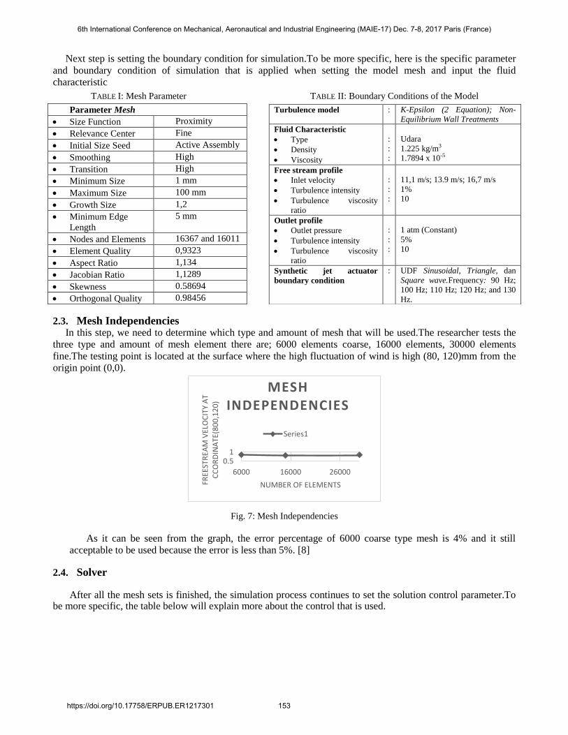
2.3. Mesh Independencies In this step, we need to determine which type and amount of mesh that will be used.The researcher tests the

three type and amount of mesh element there are; 6000 elements coarse, 16000 elements, 30000 elements

fine.The testing point is located at the surface where the high fluctuation of wind is high (80, 120)mm from the

origin point (0,0).

Fig. 7: Mesh Independencies

As it can be seen from the graph, the error percentage of 6000 coarse type mesh is 4% and it still

acceptable to be used because the error is less than 5%. [8]

2.4. Solver

After all the mesh sets is finished, the simulation process continues to set the solution control parameter.To be more specific, the table below will explain more about the control that is used.

Parameter Mesh

Size Function Proximity

Relevance Center Fine

Initial Size Seed Active Assembly

Smoothing High

Transition High

Minimum Size 1 mm

Maximum Size 100 mm

Growth Size 1,2

Minimum Edge

Length

5 mm

Nodes and Elements 16367 and 16011

Element Quality 0,9323

Aspect Ratio 1,134

Jacobian Ratio 1,1289

Skewness 0.58694

Orthogonal Quality 0.98456

Turbulence model : K-Epsilon (2 Equation); Non-

Equilibrium Wall Treatments

Fluid Characteristic

Type

Density

Viscosity

:

:

:

Udara

1.225 kg/m3

1.7894 x 10-5

Free stream profile

Inlet velocity

Turbulence intensity

Turbulence viscosity

ratio

:

:

:

11,1 m/s; 13.9 m/s; 16,7 m/s

1%

10

Outlet profile

Outlet pressure

Turbulence intensity

Turbulence viscosity

ratio

:

:

:

1 atm (Constant)

5%

10

Synthetic jet actuator

boundary condition

: UDF Sinusoidal, Triangle, dan

Square wave.Frequency: 90 Hz;

100 Hz; 110 Hz; 120 Hz; and 130

Hz.

0.51

6000 16000 26000

FREE

STR

EAM

VEL

OC

ITY

AT

CC

OR

DIN

ATE

(80

0,1

20

)

NUMBER OF ELEMENTS

MESH INDEPENDENCIES

Series1



3. Simulation Result and Discussion

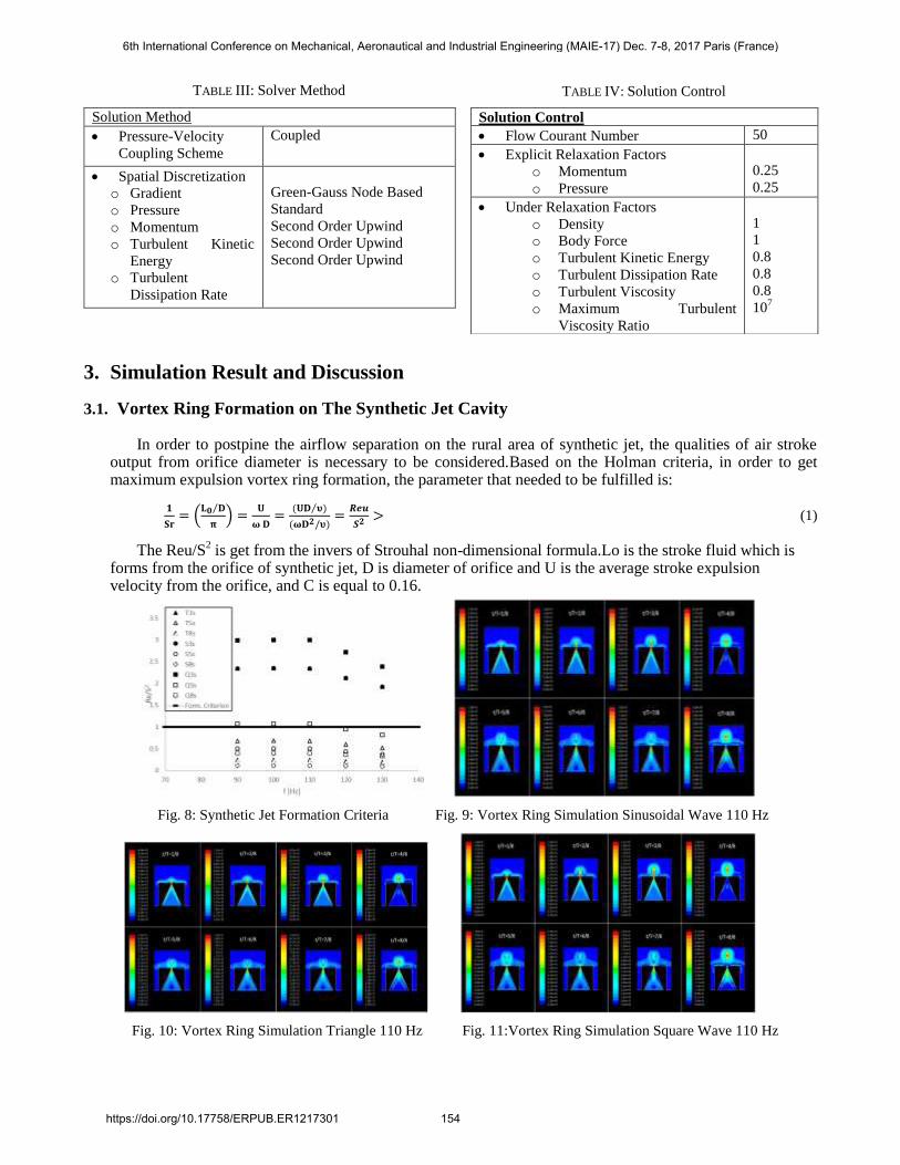
3.1. Vortex Ring Formation on The Synthetic Jet Cavity

In order to postpine the airflow separation on the rural area of synthetic jet, the qualities of air stroke output from orifice diameter is necessary to be considered.Based on the Holman criteria, in order to get maximum expulsion vortex ring formation, the parameter that needed to be fulfilled is:

(

⁄

)

⁄

(1)

The Reu/S2 is get from the invers of Strouhal non-dimensional formula.Lo is the stroke fluid which is

forms from the orifice of synthetic jet, D is diameter of orifice and U is the average stroke expulsion velocity from the orifice, and C is equal to 0.16.

Fig. 8: Synthetic Jet Formation Criteria Fig. 9: Vortex Ring Simulation Sinusoidal Wave 110 Hz

Fig. 10: Vortex Ring Simulation Triangle 110 Hz Fig. 11:Vortex Ring Simulation Square Wave 110 Hz

TABLE III: Solver Method

Solution Method

Pressure-Velocity

Coupling Scheme

Coupled

Spatial Discretization

o Gradient

o Pressure

o Momentum

o Turbulent Kinetic

Energy

o Turbulent

Dissipation Rate

Green-Gauss Node Based

Standard

Second Order Upwind

Second Order Upwind

Second Order Upwind

TABLE IV: Solution Control

Solution Control

Flow Courant Number 50

Explicit Relaxation Factors

o Momentum

o Pressure

0.25

0.25

Under Relaxation Factors

o Density

o Body Force

o Turbulent Kinetic Energy

o Turbulent Dissipation Rate

o Turbulent Viscosity

o Maximum Turbulent

Viscosity Ratio

1

1

0.8

0.8

0.8

107



Then, this Holman criteria in Figure 8 explains that the square wave signal of actuator can produce the higher vortex ring formation than the other type of signal. [9]In addition, Figure 9 explains that the Holman criteria theory is proven, when the 10 Hz square wave signal is applied to the 3 mm rifice diameter concical synthetic jet, the expulsion stroke of vortex ring velocities is 5.71 m/s. Meanwhile, In Figure 9 and 10 explain that other type of signal applied to the 3 mm conical synthetic jet produces 4.36 m/s of expulsion stroke for sinusoidal wave and 3.36 m/s of air stroke for triangle wave.

3.2. The Airflow Separation Condition After the Application of Synthetic Jet Orifice Diameter 3 mm, 5 mm, and 8 mm

3.3. A Free Stream velocity 11.1 m/s

Fig. 12: Separation Point without Synjet Jet Square wave Fig. 13: Separation Point 3 mm Synthetic jet square

Fig 14:Separation point 5 mm Synthetic Jet Square Wave Fig. 15: Separation point 8 mm Synthetic Jet Square Wave

Figure 12 shows that the airflow separation happens at (635,196) from the point origin (0,0).Then, if it is

compared to the synthetic jet which diameter 5 mm and 8 mm the longest distance of airflow separation

postponement is 3 mm cavity orifice synthetic jet.Based on the figure 13 the speartion point is moved to

(649,182) mm.

3.4. Free Stream Velocity 13.9 m/s

Fig. 16: Airflow Separation without Synjet at 13.9 m/s Fig. 17: Separation point 3 mm Synthetic Jet Square Wave

Fig. 18:Separation point 5 mm Synthetic Jet Square Wave Fig. 19: Separation point 8 mm Synthetic Jet Square Wave



When the free stream 13.9 m/s and there is no synthetic jet applied, it can be seen from figure 16 that the airflow

separation happens at(633,198)mm from x,y=(0,0).Furthermore, the figure 17 explains that the maximum

airflow separation posponement happens when the synthetic jet actuator 3 mm applied, the separation point

become (651,190) mm from the origin point.

3.5. At the Free Stream Velocity 16.7 m/s

Fig. 20: Airflow separation point at Free stream 16.7m/s Fig. 21: Separation point 3 mm Synthetic Jet Square Wave

Fig. 22: Separation point 5 mm Synthetic Jet Square Wave Fig. 23: Separation point 8 mm Synthetic Jet Square Wave

As the free flow get faster than before from 13.9 m/s to 16.7 m/s, the airflow separation will get early to happens [10] and Figure 20 shows that the airflow separation happens at (631,200)mm.When the synthetic jet actuator which orifice diameter 3 mm applied to this model.Figure 21 explains that the maximum airflow separation postponement happens and it becomes (643,188)mm from the origin point.

3.6. Drag Force Reduction

3.7. Drag Force Reduction at Free Stream 11.1 m/s

Fig. 24:Drag Reduction Percentage of Conical Cavity Orifice Diameter 3 mm, 5 mm, 8 mm

Figure 24 explain about the drag reduction through the variation of orifice diameter in free stream velocity 11.1 m/s.As it can be seen from the graph above in the 3 mm orifice diameter produces the highest drag reduction 14.2% then it follows by 5 mm orifice diameter which the drag reduction9.95% and 8 mm orifice diameter which drag reduction is 6.35%.

0.00%

5.00%

10.00%

15.00%

90 100 110 120 130

DR

AG

RED

UC

TIO

N(%

)

FREQUENCY (HZ)

DRAG REDUCTION

(3MM)DIAMETER, SQUARE

WAVE 110 HZ

K3

K5

K8



3.8. Drag Force Reduction at Free Stram 13.9 m/s

Fig. 25:Drag Reduction Percentage of Conical Cavity Orifice Diameter 3 mm, 5 mm, 8 mm

Figure 25 above explains that drag reduction of all three types orifice diameter of conical cavity synthetic jet are

rising.The 3 mm diameter has 18.62%, 5 mm has 12.21% and 8 mm has 7.34% of drag force reduction.

3.9. Drag Force Reduction at Free Stream 16.7 m/s

Fig. 26: Drag Reduction Percentage of Conical Cavity Orifice Diameter 3 mm, 5 mm, 8 mm

The graph in figure 26, explains different things happens because on the figure 24 and 25 shows that as the

velocity rises the drag reduction increase.In this free stream the 3 mm of conical cavity drag reduction is 12.48

and still remain the highest, then it follows by 5 mm which reduction is 5.99% and 8 mm diameter has 4.24 of

drag reduction.

Fig. 27: Drag reduction Percentage of 3 mm diameter conical synthetic jet

Figure 27 explains that the smallest drag reduction happens when the 3 m orifice diameter of conical cavity

synthetic jet applied the free stream velocity 16.7 m/s.Based on the fluid mechanics theory, as the free flow get

0.00%

5.00%

10.00%

15.00%

20.00%

90 100 110 120 130DR

AG

RED

UC

TIO

N

FREQUENCY (HZ)

DRAG REDUCTION PERCENTAGE

SQUARE WAVE SIGNAL(3 MM OD)

11,1 m/s

13,9 m/s

16,7 m/s

4.00%

9.00%

14.00%

19.00%

90 100 110 120 130D

RA

G R

EDU

CTI

ON

(%)

FREQUENCY (HZ)

DR AG R EDUC T IO N (3 M M )DIAM ET ER , S QUAR E W AVE

1 1 0 H Z

K3

K5

K8

0.00%

5.00%

10.00%

90 100 110 120 130DR

AG

RED

UC

TIO

N (

%)

FREQUENCY (HZ)

DRAG REDUCT ION (3 MM)DIAMET ER,

SQUARE W AVE 1 1 0 HZ

K3 K5 K8



rises, the airflow separation will get earlier to happens, so the drag force produced is high. [11]Furthermore,

since the point to take the separation poin is fixed, whether the model is not applied or applied with the

synthetic jet actuator, so it is reasonable that the higher the velocity stream, the smaller drag force reduction will

be.

3.10. Conclusion Based on the simulation result, the maximum drag force reduction is produced by the 3 mm orifice diameter of

conical cavity synthetic jet when the membrane actuator vibrate at 110 hz of square signal wave and the free

stream velocity is 13.9 m/s.The amount of drag force reduction is 18.62%.

4. Acknowledgements

This paper would not be possible to finish without the support from my institution, University of Indonesia

and the research grants from research development of University of Indonesia (PITTA).In addition the author

also indebt to all of these person in charge who always support me during the process of finishing the paper:

1. Prof. Dr. Ir. Harinaldi, M.Eng, as the author professor project advisor.The author thanks for his time to

guide the author for finishing this projects

2. Ramon Trisno, S.T, M.Eng, as the research promotor, because of his help to take the experiment and

simulation data, the time to share his knowledge about the research, this project finish before the due

date.

3. The research team, Helmy Azis, Bisma Kertanegara, Bintang Antares and Rizki Abdul Azis, who

already give their time to share the knowledge and experience for discussing our final project.

The author sincerely wishes this paper could be useful to its readers by giving valuable information. The

author fully realizes all the imperfection inside this final project. Therefore, the author humbly requests for the

readers’ criticism, feedback and suggestions to improve our future reports. We also apologize if there is any

mistakes in this paper.

5. References

[1] Munson, B, Fluid Mechanics(Translated by :Prof.Dr.Ir.Harinaldi & Ir.Budiarso, M.Eng), Jakarta: Erlangga, 2002.

[2] Olson R.M and Wright S.J, Basic Fluid Mechanics(Translated by: Alex Tri Kantjono), Jakarta: PT Gramedia

Pustaka, 1993.

[3] M. Gak-El-Hak, "Modern Development in Flow Control,," Appl. Mech. Rev., 9, pp. 365-379, 1996.

https://doi.org/10.1115/1.3101931

[4] G. R. a. G. F. Ahmed S.R., Airflow Study Through Ahmed body Model, no. 8400300-01, 1984.

[5] Versteeg & Malalasekera, Computational Fluid Dynamic The Finite Volume Method., England: Longman, 1996.

[6] Jiyuan Tu, Guan Heng Yeoh, Chaoqun Liu, Computational Fluid Dynamics, A Practical Approach, Oxford:

Elsavier, 2008.

[7] Ansys Inc, Introduction To Ansys Meshing, USA: ANSYS, 2014.

[8] Brunn A., Wassen, Sperber D, Nitsche W, and Thiele F, "Active Drag Control for a Generic Car Model," Active

Flow Controk, no. 95, pp. 247-259, 2007.

[9] Y. U. R. M. B. S. L. C. R. Holman, " ‘Formation criterion for synthetic jets’," AIAA Journal, vol. 43, no. 10, p.

2110–2116., 2005.

https://doi.org/10.2514/1.12033

[10] 2. Fares E., "Unsteady flow simulation of the Ahmed reference body using a lattice Boltzmann approach,"

Computers, and Fluids, vol. 35, pp. 940-950, 2006.

https://doi.org/10.1016/j.compfluid.2005.04.011

[11] Roumeas M, Gillieron, and Kourta A, "Analysis and Control Of the Near Wake Flow Over a Square Back

Geometry," Computers & Fluids, pp. 60-70, 2009.


[12] Lienhart H, Stoots C, and Becker S, Flow and Turbulence Structure in The Wake Of a Simplified Car

Model(Ahmed Model),Numerical and Experimental Fluid, 2002.



https://doi.org/10.1115/1.3101931

https://doi.org/10.2514/1.12033

https://doi.org/10.2514/1.12033





computational analysis orifice diameter variations effects...

Documents