computational astrophysics i: introduction and basic concepts

Computational Astrophysics I: Introduction and basic concepts

Helge Todt

AstrophysicsInstitute of Physics and Astronomy

University of Potsdam

SoSe 2021, 3.6.2021

H. Todt (UP) Computational Astrophysics SoSe 2021, 3.6.2021 1 / 32

The two-body problem


Equations of motion I

We remember (?):

The Kepler’s laws of planetary motion (1619)1 Each planet moves in an elliptical orbit where the Sun is at one of the foci of the ellipse.2 The velocity of a planet increases with decreasing distance to the Sun such, that the

planet sweeps out equal areas in equal times.3 The ratio P2/a3 is the same for all planets orbiting the Sun, where P is the orbital period

and a is the semimajor axis of the ellipse.

The 1. and 3. Kepler’s law describe the shape of the orbit (Copernicus: circles), but not thetime dependence ~r(t). This can in general not be expressed by elementary mathematicalfunctions (see below).Therefore we will try to find a numerical solution.


Equations of motion II

Earth-Sun system→ two-body problem → one-body problem via reduced mass of lighter body (partition ofmotion):

µ =M m

m + M=

mmM + 1

(1)

as mE � M� is µ ≈ m, i.e. motion is relative to the center of mass ≡ only motion of m. Setpoint of origin (0, 0) to the source of the force field of M.

Moreover: Newton’s 2. law:

md2~rdt2 = ~F (2)

and force field according to Newton’s law of gravitation :

~F = −GMmr3 ~r (3)


Equations of motion III

Kepler’s laws, as well as the assumption of a central force imply → conservation of angularmomentum →motion is only in a plane (→Kepler’s 1st law).So, we use Cartesian coordinates in the xy -plane:

Fx = −GMmr3 x (4)

Fy = −GMmr3 y (5)

The equations of motion are then:

d2xdt2 = −GM

r3 x (6)

d2ydt2 = −GM

r3 y (7)

where r =√

x2 + y2 (8)


Excursus: Analytic solution of the Kepler problem I

To derive the analytic solution for equation of motion ~r(t) → use polar coordinates: φ, r1 use conservation of angular momentum `:

µr2φ = ` = const. (9)

φ =`

µr2 (10)

2 use conservation of total energy:

E =12µr2 +

`2

2µr− GMµ

r(11)

r2 =2Eµ− `2

µ2r2 +2GM

r(12)

→ two coupled equations for r and φ


Excursus: Analytic solution of the Kepler problem II

3 decouple Eq. (10), use the orbit equation r = α1+e cosφ with numeric eccentricity e

(= f1 O/a) and α = r(π/2) ≡ `2

GMµ2 gives separable equation for φ

φ =dφdt

=G 2M2µ3

`3(1 + e cosφ)2 (13)

t =

∫ t

t0dt ′ = k

∫ φ

φ0

dφ′

(1 + e cosφ′)2 = f (φ) (14)

right-hand side integral can be looked up in, e.g., Bronstein:

t/k =e sinφ

(e2 − 1)(1 + e cosφ)− 1

e2 − 1

∫dφ

1 + e cosφ(15)

→ e 6= 1: parabola excluded; the integral can be further simplified for the elllipse:

0 ≤ e < 1 :

∫dφ

1 + e cosφ=

2√1− e2

arctan(1− e) tan φ

2√1− e2

(16)


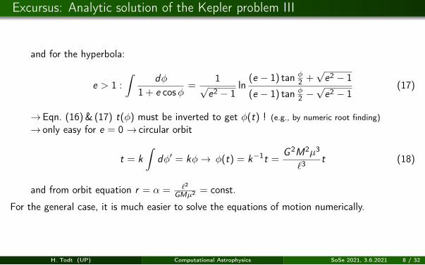
Excursus: Analytic solution of the Kepler problem III

and for the hyperbola:

e > 1 :

∫dφ

1 + e cosφ=

1√e2 − 1

ln(e − 1) tan φ

2 +√

e2 − 1

(e − 1) tan φ2 −√

e2 − 1(17)

→Eqn. (16)& (17) t(φ) must be inverted to get φ(t) ! (e.g., by numeric root finding)→ only easy for e = 0 → circular orbit

t = k∫

dφ′ = kφ→ φ(t) = k−1t =G 2M2µ3

`3t (18)

and from orbit equation r = α = `2

GMµ2 = const.

For the general case, it is much easier to solve the equations of motion numerically.


Excursus: The Kepler equation I

Alternative formulation for time dependency in case of an ellipse (0 ≤ e < 1):

A Π

Q

ψ

S

P

φ

O Ra

b

Orbit, circumscribed by auxillary circle withradius a (= semi-major axis); true anomaly φ,eccentric anomaly ψ. Sun at S , planet at P ,circle center at O. Perapsis (perhelion) Π andapapsis (aphelion) A:

consider a line normal to AΠ through P onthe ellipse, intersecting circle at Q and AΠat R .consider an angle ψ (or E , eccentricanomaly) defined by ∠ΠOQ


Excursus: The Kepler equation II

Then: position (r , φ) of the body P can be described in terms of ψ:

xP = r cosφ = a cosψ − ae (19)

yP = r sinφ = a sinψ√

1− e2 (20)

(with PR/QR = b/a =√1− e2), square both equations and add them up:

r = a(1− e cosψ) (21)

Now, to find ψ = ψ(t), need relationship between dφ and dψ, so combine Eqn. (20)& (21)

sinφ =b sinψ

a(1− e cosψ)|d/dx ′ (22)

cosφdφ =ba

(cosψ(1− e cosψ)dψ − e sin2 ψdψ)

(1− e cosψ)2 (23)

dφ =b

a(1− e cosψ)dψ (24)


Excursus: The Kepler equation III

together with the angular momentum dφ = `µr2 dt:

(1− e cosψ)dψ =`

µabdt (25)

= set t = 0→ ψ(0) = 0, integration: (26)

ψ − e sinψ =`tµab

(27)

use Kepler’s 2nd law πabP = `

2µ with πab the area of the ellipse, we get `/(µab) = 2π/P ≡ ω(orbital angular frequency), so:

Kepler’s equation

ψ − e sinψ = ωt (28)

E − e sinE = M (astronomer’s version) (29)

M: mean anomaly = angle for constant angular velocity


Excursus: The Kepler equation IV

Kepler’s equation E (t)− e sinE (t) = M(t)

is a transcendental equationcan be solved by, e.g., Newton’s methodbecause of E = M + e sinE , also (Banach) fixed-point iteration possible (slow, butstable), already used by Kepler (1621):

E = M ;for (int i = 0 ; i < n ; ++i)

E = M + e * sin(E) ;

can be solved, e.g., by Fourier series →Bessel (1784-1846):

E = M +∞∑

n=1

2nJn(ne) sin(nM) (30)

Jn(ne) =1π

∫ π

0cos(nx − ne sin x)dx (31)


Circular orbits

A special case as a solution of the equations of motion (6)& (7) is the circular orbit. Then:

r =v2

r(32)

mv2

r=

GMmr2 (equilibrium of forces) (33)

⇒ v =

√GMr

(34)

The relation (34) is therefore the condition for a circular orbit.Moreover, Eq. (34) yields together with

P =2πrv

(35)

⇒ P2 =4π2

GMr3 (36)


Astronomical units

For our solar system it is useful to use astronomical units (AU):1 AU = 1.496× 1011 m

and the unit of time is the (Earth-) year1 a = 3.156× 107 s (≈ π × 107 s),

so, for the Earth P = 1 a and r = 1AUTherefore it follows from Eq. (36):

GM =4π2r3

P2 = 4π2 AU3 a−2 (37)

I.e. we set GM ≡ 4π2 in our calculations.Advantage: handy numbers!Thus, e.g. r = 2 is approx. 3× 1011 m and t = 0.1 corresponds to 3.16 × 106 s, and v = 6.28 isroughly 30 km/s.cf.: our rcalc program with “solar units” for R , T , L; natural units in particle physics~ = c = kB = ε0 = 1 → unit of m, p, T is eV (also for E )


The Euler method I

The equations of motion (6)& (7):

d2~rdt2 = −GM

r3 ~r (38)

are a system of differential equations of 2nd order, that we shall solve now.Formally: integration of the equations of motion to obtain thetrajectory ~r(t).

Step 1: reductionRewrite Newton’s equations of motion as a system of differential equations of 1st order (here:1d):

v(t) =dx(t)

dt& a(t) =

dv(t)

dt=

F (x , v , t)

m(39)


The Euler method II

Step 2: Solving the differential equationDifferential equations of the form (initial value problem)

dxdt

= f (x , t), x(t0) = x0 (40)

can be solved numerically (discretization1) by as simple method:

Explicte Euler method (“Euler’s polygonal chain method”)1 choose step size ∆t > 0, so that tn = t0 + n∆t, n = 0, 1, 2, . . .2 calculate the values (iteration):

xn+1 = xn + f (xn, tn)∆t

Obvious: The smaller the step size ∆t, the more steps are necessary, but also the moreaccurate is the result.1I.e. we change from calculus to algebra, which can be solved by computers.


The Euler method III

Why “polygonal chain method”?

x0

x1

x2

x3

x4

x5

x6

x7

x8

0

1

2

3

4

0 1 2 3 4 5 6 7 8 9 10

t

x

Exact solution (–) and numerical solution (–).


The Euler method IV

Derivation from the Fundamental theorem of calculus

integration of the ODEdxdt

= f (x , t) from t0 till t0 + ∆t (41)∫ t0+∆t

t0

dxdt

dt =

∫ t0+∆t

t0f (x , t)dt (42)

⇒ x(t0 + ∆t)− x(t0) =

∫ t0+∆t

t0f (x(t), t)dt (43)

apply rectangle method for the integral:∫ t0+∆t

t0f (x(t), t)dt ≈ ∆t f (x(t0), t0) (44)

Equating (43) with (44) yields Euler step

x(t0 + ∆t) = x(t0) + ∆t f (x(t0), t0) (45)


The Euler method V

Derivation from Taylor expansion

x(t0 + ∆t) = x(t0) + ∆tdxdt

(t0) +O(∆t2) (46)

usedxdt

= f (x , t) (47)

x(t0 + ∆t) = x(t0) + ∆t f (x(t0), t0) (48)

while neglecting term of higher order in ∆t


The Euler method VI

For the system (39)

v(t) =dx(t)

dt& a(t) =

dv(t)

dt=

F (x , v , t)

m

this means

Euler method for solving Newton’s equations of motion

vn+1 = vn + an∆t = vn + an(xn, t)∆t (49)xn+1 = xn + vn∆t (50)

We note:

the velocity at the end of the time interval vn+1 is calculated from an, which is theacceleration at the beginning of the time interval

analogously xn+1 is calculated from vn


The Euler method VII

Example: Harmonic oscillator#include <iostream>#include <cmath>using namespace std ;

int main () {

int n = 10001, nout = 500 ;double t, v, v_old, x ;double const dt = 2. * M_PI / double(n-1) ;

x = 1. ; t = 0. ; v = 0. ;

for (int i = 0 ; i < n ; ++i) {t = t + dt ; v_old = v ;v = v - x * dt ;x = x + v_old * dt ;if (i % nout == 0) // print out only each nout step

cout << t << " " << x << " " << v << endl ;}

return 0 ;}


The Euler-Cromer method

We will slightly modify the explicit Euler method, but such that we obtain the same differentialequations for ∆t → 0.For this new method we use vn+1 for calculating xn+1:

Euler-Cromer method (semi-implicit Euler method)

vn+1 = vn + an∆t (as for Euler) (51)xn+1 = xn + vn+1∆t (52)

Advantage of this method:as for Euler method, x , v need to be calculated only once per stepespecially appropriate for oscillating solutions, as energy is conserved much better (seebelow)


Excursus: Proof of stability for the Euler-Cromer method I

Proof of stability (Cromer 1981):

vn+1 = vn + Fn∆t (= vn + a(xn)∆t, m = 1) (53)xn+1 = xn + vn+1∆t (54)

Without loss of generality, let v0 = 0. Iterate Eq. (53) n times:

vn = (F0 + F1 + . . .+ Fn−1)∆t = Sn−1 (55)xn+1 = xn + Sn∆t (56)

Sn := ∆tn∑

j=0

Fj (57)

Note that for explicit Euler Eq. (56) is xn+1 = xn + Sn−1∆t.


Excursus: Proof of stability for the Euler-Cromer method II

The change in the kinetic energy K between t0 = 0 and tn = n∆t is because of Eq. (53) andv0 = 0

∆Kn = Kn − K0 = Kn =12S2

n−1 (58)

The change in the potential energy U:

∆Un = −∫ xn

x0

F (x)dx (59)


Excursus: Proof of stability for the Euler-Cromer method III

Now use the trapezoid rule for this integral

∆Un = −12

n−1∑i=0

(Fi + Fi+1)(xi+1 − xi ) (60)

= −12

∆tn−1∑i=0

(Fi + Fi+1)Si (→ Eq. 54) (61)

= −12

∆t2n−1∑i=0

i∑j=0

(Fi + Fi+1)Fj (→ Eq. 57) (62)


Excursus: Proof of stability for the Euler-Cromer method IV

As j runs from 0 to i →∆Un has same squared terms as ∆Kn, see:

∆Un = −12

∆t2

n−1∑i=0

F 2i +

n−1∑i=0

i−1∑j=0

FiFj +n∑

i=1

i−1∑j=0

FiFj

(63)

= −12

∆t2

n−1∑i=0

F 2i + 2

n−1∑i=0

i−1∑j=0

FiFj + Fn

i−1∑j=0

Fj

(64)

= −12S2

n−1 −12

∆t FnSn−1 (65)

Hence the total energy changes as

∆En = ∆Kn + ∆Un =12S2

n−1 −12S2

n−1 −12

∆t FnSn−1 (66)

= −12

∆t FnSn−1 = −12

∆t Fnvn (67)


Excursus: Proof of stability for the Euler-Cromer method V

For oscillatory motion: vn = 0 at turning points, Fn = 0 at equilibrium points→∆En = −1

2∆t Fnvn is 0 four times of each cycle →∆En oscillates with T/2.As Fn and vn are bound →∆En is bound, more important: average of ∆En over half a cycle(T )

〈∆En〉 =∆t2

T

12T/∆t∑n=0

Fnvn '∆tT

∫ T2

0F v dt =

∆tT

∫ x( T2 )

x(0)F dx (68)

= −∆tT

(U(T/2)− U(0)) = 0 (69)

as U has same value at each turning point→ energy conserved on average with Euler-Cromer for oscillatory motion

�


Excursus: Proof of stability for the Euler-Cromer method VI

For comparison: with explicit Euler method ∆En contains term∑n−1

i=0 F 2i which increases

monotonically with n and

∆En = −18

∆t2 (F 20 − F 2

n)

(70)

with v0 = 0 →F 20 ≥ F 2

n →∆En oscillates between 0 and −18∆t2F 2

0 per cylce.Energy is bounded as for Euler-Cromer, but 〈∆En〉 6= 0


Stability analysis of the Euler method I

Consider the following ODEdxdt

= −cx (71)

with c > 0 and x(t = 0) = x0. Analytic solution is x(t) = x0 exp(−ct). The explicit Eulermethod gives:

xn+1 = xn + xn∆t = xn − cxn∆t = xn(1− c∆t) (72)

So, every step will give (1− c∆t) and after n steps:

xn = (1− c∆t)nx0 = (a)nx0 (73)

But, with a = 1− c∆t:

0 < a < 1 ⇒ ∆t < 1/c monotonic decline of xn−1 < a < 0 ⇒ 1/c < ∆t < 2/c oscillating decline of xn

a < −1 ⇒ ∆t > 2/c oscillating increase of xn !(74)


Stability analysis of the Euler method II

---- a = 0.5

---- a = -0.5

---- a = -1.01

-1.5

-1.0

-0.5

0.0

0.5

1.0

1.5

1 2 3 4 5 6 7 8 9 10

nx

n

Stability of the explicit Euler method for different a = 1− c∆t

In contrast, consider implicit Euler method (Euler-Cromer):

xn+1 = xn + xn+1∆t = xn − cxn+1∆t (75)

⇒ xn+1 =xn

1 + c∆t(76)

declines for all ∆t (!)


The Euler-Richardson method

Sometimes it is better, to calculate the velocity for the midpoint of the interval:

Euler-Richardson method (“Euler half step method”)

an = F (xn, vn, tn)/m (77)

vM = vn + an12

∆t (78)

xM = xn + vn12

∆t (79)

aM = F(

xM, vM, tn +12

∆t)/m (80)

vn+1 = vn + aM∆t (81)xn+1 = xn + vM∆t (82)

We need twice the number of steps of calculation, but may be more efficient, as we mightchoose a larger step size as for the Euler method.


Literature I

Cromer, A. 1981, American Journal of Physics, 49, 455


computational astrophysics i: introduction and basic concepts

Documents