computational biology in practice why do we work on computational biology? slides will be available...
TRANSCRIPT

Computational Biology in Practice
Why do we work on Computational Biology?
Slides will be available on
http://www.dcs.warwick.ac.uk/~feng/combio.html

Computational Biology in Practice
1. Introduction and model fitting
2. Frequency analysis
3. Network analysis

Examples: from molecular level to systems level
Microarray data (gene)
Protein data Metabolic data Neuronal data

• • • • • •
• •
Development of Arabidopsis plants during the experiment 7 showing the harvested leaf at the morning harvest

Microarray data• Measure all gene activity simultaneously • 32,000 genes in Arabdopsis leaf• One gene is responsible for senesence (aging)?

• In reality, it is a network phenomenon: many genes work together to make it happen
• Similar issues arising in all diseases: searching for biomarkers (in cancer research)
Another Example at systems level: fMRI
/ This graph shows one of these clusters enriched for Chlorophyll a b binding protein genes

Detect what you are thinking Now?
Using Fourier Transform
eye vs. ear

blood-oxygen-level-dependent (BOLD) signal

• We can record the activity of a whole brain
• To find out how a pattern: an image, a voice, an odour, is recognized in your brain
• Can we diagnosis or Prognosis a brain disease such as depression, Alzeihmer disease, epilepsy, drug addition etc.
• A huge data set (100 GB per day in a hospital) is generated and is crying for analysis

Coursework• In the coursework, two sets of data will be provided. • We have 12 subjects.• For each subject, the time series of BOLD signals
from orbitofrontal cortex (OFC) and anterior prefrontal cortex (PFC) under two conditions respectively:
pleasantness vs. intensity• For each condition, there are 9 trials with 18 time
points each (9*18=162)• Hence, the size of each matrix is 12 * 162.

From the data http://www.dcs.warwick.ac.uk/~feng/combio/Work out the causal relationship between two
conditions

• Attempt all parts and submit a report that should include the program listings (with comments).
• Please visit the following web site for a
submission cover sheet:
http://www.dcs.warwick.ac.uk/undergraduate/cover.html
• Completed report should be submitted to the
filing cabinet in the Terminal Room CS006 in the Computer Science Department before 1700 hour on Monday Week 10 (i.e., 14th March 2011).

Problems with fMRI
• Very poor temporal resolutions (neuronal activity at msec level, fMRI at sec level)
• In conjunction with EEG etc.

Brain machine interfaceA brain-computer interface (BCI), sometimes called a direct
neural interface or a brain-machine interface, is a direct communication pathway between a brain and an external device.
In one-way BCIs, computers either accept commands from the brain or send signals to it (for example, to restore vision) but not both.
Two-way BCIs would allow brains and external devices to exchange information in both directions but have yet to be successfully implanted in animals or humans.

Dial a mobile automatically

• Pharmacological treatments

Parkinson’s disease• In neurotechnology, deep brain stimulation (DBS) is a surgical
treatment involving the implantation of a medical device called a brain pacemaker, which sends electrical impulses to specific parts of the brain.
• DBS in select brain regions has provided remarkable therapeutic benefits for otherwise treatment-resistant movement and affective disorders such as chronic pain, Parkinson’s disease, tremor and dystonia.
• Despite the long history of DBS, its underlying principles and mechanisms are still not clear.
• DBS directly changes brain activity in a controlled manner, its effects are reversible (unlike those of lesioning techniques) and is one of only a few neurosurgical methods that allows blinded studies.


One of our own stories

Oxytocine is a hormone released in your brain Oxytocin=Greek: "quick birth“, hormone
Hypothalamus

Science 2005

• Assumption: The rhythm arises from the synergistic interaction between intrinsic and synaptic properties of the component neurons
• Two extreme mechanisms:– Component neurons are intrinsic oscillators. They act as pacemakers for the network– Component neurons are not intrinsic oscillators. The rhythm arises from synaptic interactions– Usually, there is a blend of both strategies
• Neurons are intrinsic oscillators• Reciprocal inhibition: a common connectivity pattern• Pacemaker kernel sets the pace• Synapses control frequency (partially) and phase
sequence• CPGs: They transform excitation into a
rhythmic pattern by appropriate spatio-temporal distribution of inhibition
• A pool of spiking interneurons• Excitatory interconnections between them
create a positive feedback loop that transforms an external tonic excitatory input into a burst
• The burst terminates intrinsically, after accumulation of intracellular signal (calcium) and activation of IK(Ca)
Network oscillators
Emergent activity


Synchronization is an emergent activity


Common theme
• Dealing with data with time
• Dynamical System
Machine learning, a branch of artificial intelligence, is a scientific discipline concerned with the design and development of algorithms that allow computers to evolve behaviors based on empirical data, such as from sensor data or databases.
A learner can take advantage of examples (data) to capture characteristics of interest of their unknown underlying probability distribution.
Data can be seen as examples that illustrate relations between observed variables.
A major focus of machine learning research is to automatically learn to recognize complex patterns and make intelligent decisions based on data; the difficulty lies in the fact that the set of all possible behaviors given all possible inputs is too large to be covered by the set of observed examples (training data).

Hence the learner must generalize from the given examples, so as to be able to produce a useful output in new cases.
Machine learning, like all subjects in artificial intelligence, requires cross-disciplinary proficiency in several areas, such as probability theory, statistics, pattern recognition, cognitive science, data mining, adaptive control, computational neuroscience and theoretical computer science.
In the next three weeks, we will learn one technique to tackle one single issue

Mathematical BackgroundDefinition• A VAR model describes the evolution of a set of k variables over
the same samples period (t = 1, ..., T) as a linear function of only their past evolution.
• The variables are collected in a k × 1 vector y(t), which has as the ith element yi the time t observation of variable yi. For example, if the ith variable is the ith gene activity, then yi is the value of gene activity at t.
• A p-th order VAR, denoted VAR(p), is

tp ptYAtYAAtY )()1()( 10

where A0 is a k × 1 vector of constants, Ai is a k × k matrix (for every i = 1, ..., p) and et is a k × 1 vector of error terms satisfying
— every error term has mean zero; — the contemporaneous covariance matrix of error terms is S (a k × k positive definite matrix); — for any non-zero k , there is no correlation across time; in particular, no serial correlation in individual error terms. • The l-periods back observation y(t-l) is called the l-th lag of y. Thus, a pth-order VAR is also called a VAR with p lags.

Normal distributionWe usually assume that the error term is
normally distributed
et ~ N(m,s)
et ~ N(m,S)

• x=randn(1,1000);• hist(x)• clear all• x=randn(2,1000);• s=[2 1; 1 2];• sqrt(s)*sqrt(s)• y=x'*sqrt(s);• cov(y)• (this actually has a problem, can you
correct it)

Graphic representations
x1
x5
x2
x6x4
x3

Stationary
• What do we need?• Y = a y + et
a < 1 a = 1 a > 1
How to deal with it in matrix case?

ntYAtY )1()( 1
It is stationary if and only if all eigenvalues of the matrix A1 is inside the unit circle, i.e. |eig(A1)|<1
Example 1: clear allclose allk=2;A=rand(k,2);x=zeros(1000,k);x(1,:)=rand(1,k)';for i=1:1000 x(i+1,:)=(A*x(i,:)')'+rand(1,k);endplot(x(:,1))hold onplot(x(:,2),'r')abs(eig(A))

How to deal with general case
• Linear system is always easy to deal with
• We can simply enlarge the state space so that it become VAR(1)

Map VAR(p) to VAR(1)
t
t
t
tp
tAXtX
ty
tyaa
ty
ty
tyatyaty
ptYAtYAAtY
)1()(
0)2(
)1(
01)1(
)(
)2()1()(
)()1()(
21
21
10

• clear all• close all• A1=rand(2,2)*0.5;• A2=rand(2,2)*0.5;• I=[1 0;0 1];• x=zeros(1000,2);• y=zeros(1000,2);• y(1,:)=rand(1,2)';• x(1,:)=rand(1,2)';• x(2,:)=rand(1,2)';• for i=1:999• y(i+1,:)=(A1*y(i,:)')'+rand(1,2); • end• for i=1:998• x(i+2,:)=(A1*x(i+1,:)')'+(A2*x(i,:)')'+rand(1,2); • end• figure(1)• plot(x(:,1))• hold on• plot(x(:,2),'r')• figure(2)• plot(y(:,1))• hold on• plot(y(:,2),'r')• abs(eig(A1))• abs(eig(A2))• A=[A1 A2;I,0*I];• abs(eig(A))

The difference
0 100 200 300 400 500 600 700 800 900 10000
1
2
3
4
5
6
7
8
9
10
0 100 200 300 400 500 600 700 800 900 10000
0.5
1
1.5
2
2.5

• >> mean(x)
• ans =
• 7.1078 7.5605
• >> cov(x)
• ans =
• 0.7840 0.7552• 0.7552 0.9193
• >> mean(y)
• ans =
• 1.3921 1.0293
• >> cov(y)
• ans =
• 0.1290 0.0230• 0.0230 0.0972

0 10 20 30 40 50 60 70 80 90 100-0.2
-0.1
0
0.1
0.2
0.3
0.4
0.5
0.6
0.7
for i=1:100 cc=corrcoef(x([100:500],1),x([100+i:500+i],1)); cx(i)=cc(1,2); cc=corrcoef(y([100:500],1),y([100+i:500+i],1)); cy(i)=cc(1,2); endplot(cx)hold onplot(cy,'r')

For z=yj, x=yi,
Rxx(t)= cov (x(t) x(t+t))/ [SD(x(t)) SD(x(t+t ))]
Autocorrelation with lag t
Rxz(t)=
Crosscorrelation with lag t

Other issues

nonstationary
• y(t+1)= c t + y(t)+ e(t)

Beyond linear model
• Communication in brain
Neuron 1
Neuron 2
1 0 0 1 0 1 0 1 1 0 0
1 0 0 0 0 0 0 0 0 1 1

Beyond linear model
• Communication in brain
Neuron 1
Neuron 2
1 0 1 0 0 1 0 1 1 0 0
1 0 0 0 0 0 0 0 0 1 1

Using kernal function to replace A y(t-l)

Seminar 1
• Generate a two-dimensional VAR(2) time series (x(t), y(t)), t=1,…1000, using Matlab
• Check whether it is stationary or not• Using graphic representation to draw the
interactions between (x(t), y(t))• Given (x(t),y(t)), can you think a way to find the
coefficients in VAR(2)?

The second week
• Given you a set of recorded data, how can we fit it with a VAR(p) model?
x(t)= a x(t-1) +b y(t-1) + e1
y(t)= c x(t-1) +d y(t-1) + e2

Let us look at the one-dim case first
x(t)= a x(t-1) +e1

Least Square fitting (regression)
X(t)
Recorded data
Find this line
X (t-1)

Error function E = sumt (x(t)-ax(t-1))2
• To find a coefficient a such that the error function is minimized
(least square fitting)
• Take the derivative with respect to a 0 = sum (x(t)-ax(t-1))x(t-1) a = [sum x(t)x(t-1)]/ [sum x(t-1)x(t-1)]

clear all close allh=0.1;a=0.5;for i=1:1000 x(i)=h*i; % time z(i)=a*x(i); % actual relationship y(i)=a*x(i)+4*randn(1,1); % experimental observed dataendplot(x,y,'*')hold onplot(x,z,'r')a_bar=(x*y')/(x*x')plot(x,a_bar*x,'g')

In matrix format
a = (X Y’)/ (X X’)= (Y X’) * (X X’)-1
X = (X1, X
2, X
3, …, X
N) recorded data
Y= (y1, y2, …, yN)
For VAR(1) Y = A Y + epsilonA = (Y(t)Y(t-1)’)(Y(t-1)*Y(t-1) ’)-1
Y (t) = (Y1, Y
2, …, Y
N) recorded data
Y(t-1)= (Y1, Y2, …, YN) (there is one error here)

• clear all• close all• k=2;• N=1000;• A=rand(k,2);• x=zeros(N+1,k);• x(1,:)=rand(1,k);• for i=1:N• x(i+1,:)=(A*x(i,:)')'+randn(1,k);• end• plot(x(:,1))• hold on• plot(x(:,2),'r')• abs(eig(A))• A• AE=(x([11:N],:)'*x([10:N-1],:))*(inv(x([10:N-1],:)'*x([10:N-1],:)))

• A =
• 0.1190 0.9597• 0.4984 0.3404
• AE =
• 0.1363 0.9308• 0.4839 0.3618

Graphic representation
Note that here I do not use the first 9 points of data since it is not stationary.
For experimental data, you could use them all.

Finally, we can estimate S S = = cov [Y(t)-Ahat*Y(t-1) ] • clear all• close all• k=2;• N=1000;• A=rand(k,2);• x=zeros(N+1,k);• x(1,:)=rand(1,k);• for i=1:N• x(i+1,:)=(A*x(i,:)')'+randn(1,k);• end• plot(x(:,1))• hold on• plot(x(:,2),'r')• abs(eig(A))• A• AE=(x([11:N],:)'*x([10:N-1],:))*(inv(x([10:N-1],:)'*x([10:N-1],:)))• cov(x([11:N],:)-(AE*x([10:N-1],:)')')

Write down its VAR equation
A =
0.5472 0.1493 0.1386 0.2575
AE =
0.5689 0.0826 0.1380 0.2988
ans =
1.0377 0.0395 0.0395 1.0454

tp ptYAtYAAtY )()1()( 10
Tomorrow, during seminar, you are asked to work
this out with matlab
Bring your labtop with you
Your assignment:
Homer Simpson brain wallpaper. Free desktop wallpaper download 1024 x 768. Right click on image and select: "Set as background". If you prefer to save the image in your pc select "Save image as" instead. It
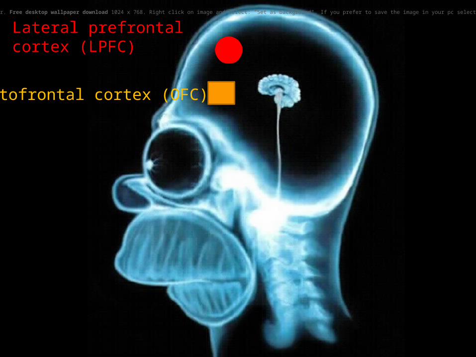
Lateral prefrontal cortex (LPFC)
Obitofrontal cortex (OFC)

Homer Simpson brain wallpaper. Free desktop wallpaper download 1024 x 768. Right click on image and select: "Set as background". If you prefer to save the image in your pc select "Save image as" instead. It
cookies
Lateral prefrontal cortex (LPFC)
Obitofrontal cortex (OFC)

Homer Simpson brain wallpaper. Free desktop wallpaper download 1024 x 768. Right click on image and select: "Set as background". If you prefer to save the image in your pc select "Save image as" instead. It
cookies
Lateral prefrontal cortex (LPFC)
Obitofrontal cortex (OFC)
Pay attention to Pleasantness to the food in your mind

x=load('fMRI.mat'); 12 individuals with a recording of 162 pointsx =
OFCpleas: [12x162 double] LPFCpleas: [12x162 double] OFCintens: [12x162 double] LPFCintens: [12x162 double]
plot(x.OFCpleas(1,:))
0 20 40 60 80 100 120 140 160 180-50
-40
-30
-20
-10
0
10
20
30
40
50

plot(x.LPFCpleas(1,:))
0 20 40 60 80 100 120 140 160 180-100
-80
-60
-40
-20
0
20
40
60
80
Question: Is there a causal driving from LPFC to OFC?

Homer Simpson brain wallpaper. Free desktop wallpaper download 1024 x 768. Right click on image and select: "Set as background". If you prefer to save the image in your pc select "Save image as" instead. It
cookies
Lateral prefrontal cortex (LPFC)
Obitofrontal cortex (OFC)
Pay attention to pleasantness to the food in your mouth
Is there a causal relationship?

Homer Simpson brain wallpaper. Free desktop wallpaper download 1024 x 768. Right click on image and select: "Set as background". If you prefer to save the image in your pc select "Save image as" instead. It
cookies
Lateral prefrontal cortex (LPFC)
Obitofrontal cortex (OFC)
Pay attention to pleasantness to the food in your Mouth
Pay attention to Intensity to the food in your Mouth
Is there a causal relationship

0 20 40 60 80 100 120 140 160 180-100
-80
-60
-40
-20
0
20
40
60
80
100
0 20 40 60 80 100 120 140 160 180-150
-100
-50
0
50
100
150

• In your assignment, we should only look at VAR(1);
• In general, it is not VAR(1), but VAR(p)

Model Fitting• As we have shown before, we can do a pretty good
job to find all parameters in the model if we know the model structure
• In the literature, the approach above is called parametric estimate
• In general, we have no clue on the model structure
• Assume it is VAR (p), how to decide the key parameter p?


AIC
• Akaike's information criterion, developed by Hirotsugu Akaike under the name of "an information criterion" (AIC) in 1971 and proposed in Akaike (1974), is a measure of the goodness of fit of an estimated statistical model.
• It is grounded in the concept of entropy, in effect offering a relative measure of the information lost when a given model is used to describe reality and can be said to describe the tradeoff between bias and variance in model construction, or loosely speaking that of precision and complexity of the model.

AIC• Intuitively speaking we replace the error function E by Etotal = E + p
or specifically AIC= 2p+T[log(2 pi E/T)+1]
• In practice, we plot AIC vs. p and select the order p as the minimal point of AIC
• This is an interesting idea and quite popular under the umbrella Bayesian approach: we fit the model, but also select the model

• One might argue that the longer the VAR model is, the better for us since we can certainly fit the data better with a longer model
• However, this could be very misleading since a longer model could simply fit the noise (overfitting)
• The extra term in AIC is usually called penalty term: which prohibits a long, overfitting model.

Example• Let us look at a simple example• y(t+1)=a1 y(t)+a2 y(t-1)+…ap y(t-p) + et
0
0
)(
)1(
)(
0
.
0
1...00
......
0...01
0...
)1(
)(
)1( 21
tp
pty
ty
tyaaa
pty
ty
ty

0 200 400 600 800 1000 1200-4
-3
-2
-1
0
1
2
3
4
1 1.5 2 2.5 3 3.5 4 4.5 5 5.5 64.5
5
5.5
6
6.5
7
7.5
8
8.5
9

• clear all• close all• k=1;• N=1000;• A=rand(1,1);• x=zeros(N+1);• x(1)=rand(1,1);• for i=1:N• x(i+1)=A*x(i)+randn(1,1);• end• plot(x(:,1))• hold on• • • T=6;• • for k=1:T• y=zeros(N+1,k);• M=floor(N/k);• for m=1:M• for n=1:k• y(m,n)=x(m*k+n);• end• end• • AE=(y([11:N-9],:)'*y([10:N-10],:))*(inv(y([10:N-10],:)'*y([10:N-10],:)))• E=cov(y([11:N-9],:)-(AE*y([10:N-10],:)')')• • AIC(k)=k*2+k*[log(2*pi*E(1,1)/k)+1] • clear y• end

Other issues
pp ptYAtYAAtY )()1()( 10
1. Treat A0 as a dumn variable, i.e. input is always 1
2. Detrend for example, use y(t)=x(t)-x(t-1) so that it becomes stationary
3. There are other ways to estimate the model such as MLE and dynamical Bayesian netwoks

MLE (maximal likelihood estimate) EM is a special case
Dynamical Bayesian Network possible the most popular approach at moment

Bayesian rule P(B|A)= P(B A)/P(A) = P(A|B) / P(A) In Bayes' theorem, each probability has a conventional name:• P(A) is the prior probability of A. It is "prior" in the sense that it does not take into account
any information about B; however, the event B need not occur after event A. The unconditional probability P(A) was called "a priori" by Ronald A. Fisher.
• P(A|B) is the conditional probability of A, given B. It is also called the posterior probability because it is derived from or depends upon the specified value of B.
• P(B|A) is the conditional probability of B given A. It is also called the likelihood.
• P(B) is the prior or marginal probability of B, and acts as a normalizing constant.

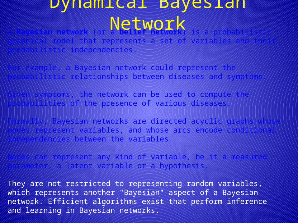
Dynamical Bayesian NetworkA Bayesian network (or a belief network) is a probabilistic graphical model that represents a set of variables and their probabilistic independencies.

Dynamical Bayesian NetworkA Bayesian network (or a belief network) is a probabilistic graphical model that represents a set of variables and their probabilistic independencies. For example, a Bayesian network could represent the probabilistic relationships between diseases and symptoms.

Dynamical Bayesian NetworkA Bayesian network (or a belief network) is a probabilistic graphical model that represents a set of variables and their probabilistic independencies. For example, a Bayesian network could represent the probabilistic relationships between diseases and symptoms. Given symptoms, the network can be used to compute the probabilities of the presence of various diseases.

Dynamical Bayesian NetworkA Bayesian network (or a belief network) is a probabilistic graphical model that represents a set of variables and their probabilistic independencies. For example, a Bayesian network could represent the probabilistic relationships between diseases and symptoms. Given symptoms, the network can be used to compute the probabilities of the presence of various diseases.
Formally, Bayesian networks are directed acyclic graphs whose nodes represent variables, and whose arcs encode conditional independencies between the variables.
Nodes can represent any kind of variable, be it a measured parameter, a latent variable or a hypothesis.
They are not restricted to representing random variables, which represents another "Bayesian" aspect of a Bayesian network. Efficient algorithms exist that perform inference and learning in Bayesian networks.
Bayesian networks that model sequences of variables (such as for example speech signals or protein sequences) are called dynamic Bayesian networks.

Seminar 2
• Generate a two-dimensional VAR(1) time series x(t), t=1,…1000, using Matlab
• Given x(t), find the method to fit it using VAR(1).
• Plot AIC (p) for p=1,2,…

The third week: causality analysis


Granger causality: network structure
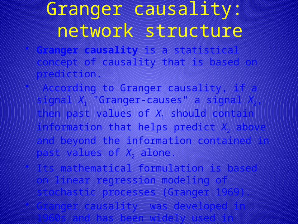
• Granger causality is a statistical concept of causality that is based on prediction.
•

Granger causality: network structure
• Granger causality is a statistical concept of causality that is based on prediction.
• According to Granger causality, if a signal X1 "Granger-causes" a signal X2, then past values of X1 should contain information that helps predict X2 above and beyond the information contained in past values of X2 alone.
• Its mathematical formulation is based on linear regression modeling of stochastic processes (Granger 1969).
• Granger causality was developed in 1960s and has been widely used in economics since the 1960s.
• However it is only within the last few years that applications in biology have become popular.

Prof. Clive W.J. Granger, recipient of the 2003 Nobel Prize in Economics

• The topic of how to define causality has kept philosophers busy for over two thousand years and has yet to be resolved.

• The topic of how to define causality has kept philosophers busy for over two thousand years and has yet to be resolved.
• It is a deep convoluted question with many possible answers which do not satisfy everyone, and yet it remains of some importance.

• The topic of how to define causality has kept philosophers busy for over two thousand years and has yet to be resolved.
• It is a deep convoluted question with many possible answers which do not satisfy everyone, and yet it remains of some importance.
• Investigators would like to think that they have found a "cause", which is a deep fundamental relationship and possibly potentially useful.
• In the early 1960's I was considering a pair of related stochastic processes which were clearly inter-related and I wanted to know if this relationship could be broken down into a pair of one way relationships.
• It was suggested to me to look at a definition of causality proposed by a very famous mathematician, Norbert Wiener, so I adapted this definition (Wiener 1956) into a practical form and discussed it.
• Applied economists found the definition understandable and useable and applications of it started to appear.

Mathematical definition• Give you a set of data, (x(t),y(t))• Fit the data with x(t) = a0 +a11 x(t-1)+…+a1p x(t-p)
+ b11 y(t-1) + … +b1p y(t-p)+ e1t
y(t) = a0 +a21 x(t-1)+…+a2p x(t-p)
+ b21 y(t-1) + … +b2p y(t-p)+ e2t
andx(t) = c0 +c11 x(t-1)+…+c1p x(t-p) + x1t
y(t) = d0+ d21 y(t-1) + … +d2p y(t-p)+ x2t

• y(t) is a Granger cause of x(t) if and only if var (x(1t)) > var (e1t)
or FY->X =log[var (x(1t))/ var (e1t)]>0

• clear all• close all• k=2;• N=1000;• A=rand(k,2);• x=zeros(N+1,k);• x(1,:)=rand(1,k);• for i=1:N• x(i+1,:)=(A*x(i,:)')'+randn(1,k);• end• plot(x(:,1))• hold on• plot(x(:,2),'r')• abs(eig(A))• A• AE=(x([11:N-9],:)'*x([10:N-10],:))*(inv(x([10:N-10],:)'*x([10:N-10],:)))• co=cov(x([11:N-9],:)-(AE*x([10:N-10],:)')');• AE_Granger=[AE(1,1) 0; 0 AE(2,2)];• cog=cov(x([11:N-9],:)-(AE_Granger*x([10:N-10],:)')');• A(1,2)• F_Y_to_X=log(cog(1,1)/co(1,1))• A(2,1)• F_X_to_Y=log(cog(2,2)/co(2,2))

Graphical representation
x Y

Underlying mechanism
• Consider two oscillators; according to the definition above, we can assess the causality in terms of their phases.
• Without noise, it actually doe not work

Other issues• Conditional Granger causality: this could
create a false causality as indicated in dashed line
x Y
Z

Common inputs
• Partial Granger causality: get rid of common inputs

Granger causality in the frequency domain

DFT


w = 2 p k /N
y1=[ 0.8900 0.2838 -0.5071 -3.2185 -1.4326 -3.4192 -2.2660 0.0836 -0.4860 0.8500 -0.7345 -0.5103 0.0445 -0.8006 -2.2613 -3.2948 -2.7340 -1.1170 -5.0842 -3.2483 -1.9090 -1.6674 -3.6872 -4.8392 -1.6104 -1.7963 -2.7653 -3.4246 -1.2610 -1.6252 -2.2733 -1.3700 -1.9442 -2.4821 -1.5835 -1.2642 -2.2062 -0.4804 -0.7040 -0.9342 -1.4635 -1.4217 6.5222 6.3718 6.7612 6.0387 5.4644 4.5623 4.0823 4.3750 4.3987 3.1775 5.3271 4.5798 4.7708 5.5316 -1.3237 -0.6287 -0.0831 -0.7494 1.6089 1.4772 4.0095 5.1718 4.3305 4.2560 -0.8167 3.4848 -1.2116 -0.9308 -3.3943 -3.5389 -1.9443 -1.2607 -1.6920 -2.1766 1.0187 -3.9071 0.4885 -0.0559 -1.4321 -1.8300 -1.4688 -0.7473 1.0083 2.0168 1.9618 1.2593 1.0622 0.9995 0.1974 1.4279 -0.1218 -0.4965 0.6089 0.6683 0.6824 0.7250]
y2=[ -1.5913 -1.2817 -1.3978 -2.6073 -1.6096 -2.2538 -2.1967 -0.8356 0.1223 -0.0290 0.9207 0.5348 -1.6927 -0.9019 -0.4397 -1.7727 -0.3895 -2.9369 -1.8197 -1.4024 -1.2942 -2.2497 -1.6920 -2.1951 -1.3292 -3.2368 -1.7904 -5.6058 -0.4675 -1.8217 -0.9824 -1.0972 -3.0887 -1.0896 -0.9148 -0.5404 -0.6809 -1.2174 -1.1689 -2.1717 -1.4879 -1.2714 5.6686 5.2338 4.8899 4.3310 4.3029 4.0934 3.9316 4.0582 3.4541 4.3231 6.5551 5.0166 6.4040 5.7404 -0.8376 -0.3785 -0.1525 0.8483 1.4076 2.0669 1.6937 0.9976 0.2318 -0.1276 -0.6031 -0.8685 -0.9742 0.4361 -0.6423 -2.4989 -0.4678 -0.4112 -2.1789 -0.6642 -1.8729 -1.8501 -3.6220 -2.7233 -2.0927 -2.3362 -2.6892 -2.0804 -0.0869 0.3587 0.3066 0.1804 -0.8788 -0.9222 0.3760 0.3186 -1.0846 -0.0598 1.6312 2.0180 1.4028 1.1970]
y3=[ -1.1113 -1.9326 -1.4380 -0.8197 -0.8968 0.6573 0.3927 0.6171 -0.4798 -1.2617 -2.3358 -1.3001 -1.8011 -1.3819 -3.3258 -3.1756 -1.7946 -1.7474 -2.7476 -1.2220 -1.2636 -2.9803 -5.9419 -3.8438 -3.6448 -2.3834 -5.4058 -1.8657 -2.7681 -2.5307 -3.3997 -0.8484 -1.0405 -0.3215 -1.3437 -0.0541 -1.2571 -1.4978 -1.7199 -1.7060 -1.3403 -1.1315 5.4301 4.7638 5.3986 4.1592 3.4255 3.6753 3.4875 4.6781 5.7853 5.7093 5.0430 5.6310 5.2887 4.4429 0.6090 2.2569 3.2070 3.3116 4.4651 4.0356 0.9805 -0.1327 -1.1654 -0.9366 -0.9429 0.2230 -0.5696 0.8233 -2.0805 -1.0515 0.3200 0.2602 1.0182 0.7138 -1.7947 -2.2518 -1.2495 -2.8302 -2.8656 -1.9344 -2.7324 -1.6842 0.9664 0.8560 0.8444 -0.2847 -0.5304 -0.7475 -0.0495 0.8815 0.8153 0.4531 0.7130 0.4842 1.1053 0.3536]
y4=[ -1.5629 -1.3146 -2.3187 -1.4200 -1.0698 -0.8720 -0.0581 -0.7040 -0.9083 -0.1637 -1.2387 -1.9663 -1.3931 -1.2987 -0.4419 -2.7723 -2.8456 -1.2274 -1.8841 -2.1944 -3.1944 -4.3064 -5.1124 -1.5171 -3.8637 -2.0934 -3.3278 -2.1742 -2.3531 -0.8733 -1.5454 -0.0722 -1.0644 -0.6315 -1.3939 -0.1475 -1.0830 -1.0649 -1.0840 -1.7295 -1.6956 -1.9917 3.9664 4.0987 3.7499 3.5711 3.8516 4.4219 5.3178 7.0641 5.4455 5.9487 4.8179 4.6775 4.0155 3.7352 2.1015 2.5427 1.7401 2.5474 0.1965 -0.3423 -0.6708 -0.5742 -0.8653 -0.1119 2.3379 2.5526 4.3619 4.2544 -0.6022 -0.9067 -1.5457 -0.7688 -2.1087 -1.4132 -1.7204 -1.7984 -2.2909 -2.4285 -0.3714 -0.6466 1.0687 1.1565 0.0567 -0.0342 -1.8122 -1.1068 -0.2483 0.1029 0.9543 1.5397 1.7971 1.9175 0.8227 0.7427 0.3243 0.0947]
y5=[0.0852 1.4502 1.1921 1.3107 0.7164 -0.0542 0.2408 -0.8628 -0.6566 -1.6902 -1.1169 -1.8113 -0.8302 -0.4098 -2.3219 -3.3268 -2.3250 -1.8097 -5.3647 -5.5535 -4.8778 -2.9077 -1.7377 -1.5831 -2.9420 -1.2204 -0.7912 -2.0745 -1.4007 0.8742 0.2277 -0.9107 -2.8332 -1.1125 -0.6868 -2.0465 -1.6175 -1.3025 -0.8161 -2.0731 -0.6975 -1.0642 3.4434 3.0369 3.5191 3.5191 4.8164 5.8171 4.9752 5.1282 4.8684 4.4455 3.9173 3.8393 4.0938 3.8839 4.3790 3.1935 0.8013 -0.9428 -0.2171 -1.0597 -0.5462 -0.9369 0.1001 1.3242 1.5758 1.9678 1.6801 2.5483 1.0797 0.8469 -0.4669 -1.3864 -2.6224 -1.6965 -1.9245 -1.9346 -3.1694 -1.4811 -1.5022 -1.5644 -0.8952 0.4871 -1.6433 -0.1679 0.3653 -1.0544 0.8967 1.0900 1.0151 0.6483 0.4187 0.7921 -0.1515 -0.0602 -0.2658 -0.3170]
y6=[-0.8652 0.0036 1.1084 -0.2068 -0.3005 -1.5268 -1.8371 -0.2243 -1.7261 -1.2691 -0.0821 0.6196 1.2519 1.2866 -6.0917 -2.0125 -1.9691 -5.2339 -1.9105 -3.3723 -3.2504 -2.8142 -1.2481 -2.3068 -2.4571 -2.6644 -4.7704 -2.1349 -1.1946 -1.2071 -1.9251 -1.1168 -1.3249 -1.4142 -1.1509 -1.1490 -1.4723 -2.0390 -1.3886 -0.4793 0.2396 -1.0024 3.5687 4.5179 5.9633 5.9080 5.4796 6.1459 5.5720 4.5894 4.0429 4.0128 3.2153 4.2673 3.5794 3.9240 0.0859 -0.1722 -0.4743 -0.8890 -1.0859 0.2596 2.1846 3.6090 3.5600 5.4268 5.2363 3.3346 0.7492 -0.2753 -1.1376 -1.4963 -1.8902 -1.7854 -0.8973 -2.2627 -1.1146 -0.7461 -0.2912 1.3372 1.4405 -0.1810 -1.4463 -2.1352 -0.4468 0.2502 1.7787 1.0989 1.4883 1.3513 1.0341 0.4089 0.4600 0.0967 -0.3997 -0.5862 -0.2064 0.2938]
y7=[ 0.4973 -0.1411 -0.7166 -0.7245 -1.5123 -1.6645 0.4459 -0.9774 -1.4978 -0.1646 -0.2848 -0.9623 -1.8286 -2.3521 -1.4760 -5.7693 -1.0593 -5.1050 -2.6712 -2.8494 -1.3592 -1.1994 -3.2579 -2.7392 -0.7956 -1.0756 -1.8185 -0.6120 -1.3946 -1.8223 -4.1718 -1.2683 -1.3835 -0.2097 -0.7923 -1.5900 4.9942 5.0916 5.2036 4.5940 4.6480 4.3785 4.3163 4.0018 3.9734 3.9739 3.5365 4.1441 -1.0877 -0.7001 -0.9794 -1.0045 -0.0221 1.6507 1.3964 2.3687 2.7116 2.5239 1.4007 -1.5811 -1.9969 -1.9188 -2.8198 -1.1193 -2.1052 -1.3470 -2.2429 -0.4253 -0.7935 0.0385 -2.3621 -2.0373 0.2646 0.7820 0.9164 -0.8839 0.6421 0.7783 1.2660 -0.2134 -0.5567 -0.6312 0.0221 -0.2545]
Y=[y1 y2 y3 y4 y5 y6 y7]
Infected one
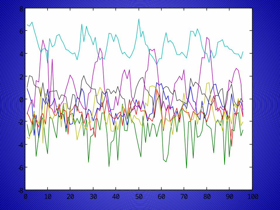
0 10 20 30 40 50 60 70 80 90 100-8
-6
-4
-2
0
2
4
6
8

• X1=[ 1.0190 0.1570 -0.1225 -0.8800 -1.4928 -1.7902 -3.1778 -1.6361 -0.7156 0.8316 1.9254 1.8985 1.9387 • -1.9694 -2.9392 -2.1622 -1.7299 -2.0305 -3.2254 -3.0013 -1.2102 -3.3928 -2.4707 -2.9994 -1.6038 -2.1691• -0.9249 -1.7333 -1.6734 -1.6082 -2.7585 -1.2762 -2.0447 -1.7753 -1.3215 -0.2138 0.6119 -0.5232 -1.1280• 6.2650 5.4346 6.4374 5.1656 5.3450 4.4928 4.1700 3.4881 3.7927 3.1822 3.4520 4.8187 6.0609• -0.4206 -0.6571 -0.5695 0.6961 2.6557 2.3846 3.7432 5.1207 5.4658 5.1733 0.5150 -0.0293 -0.8512• -0.8917 -1.5081 -3.9777 -0.8279 -0.7752 -1.5570 -1.1957 1.3889 1.1591 1.5366 -1.7075 -1.8569 -1.4095• 1.3467 1.5135 1.6885 1.0998 1.0617 1.0890 0.5793 -0.4426 0.1109 -0.5715 0.0801 0.6778 1.9681]
• X2=[ 0.0975 0.8302 -0.4235 -1.4994 -0.3467 -0.7689 -0.2982 -1.5088 0.4120 1.5100 0.6821 0.5272 -0.3992• -2.2854 -3.6403 -1.7551 -1.9432 -2.3596 -3.9362 -1.2242 -5.4418 -2.0289 -1.4007 -2.8160 -3.1527 -1.1349• -1.0630 -1.6152 -1.4750 -1.1032 -1.1556 -1.4670 -1.5154 -1.0782 0.1998 0.5478 -0.2117 -1.7717 -1.2288• 5.8870 6.7253 5.5394 4.8081 4.5301 4.6393 4.1688 3.6951 3.5569 3.3128 4.5196 6.1852 5.4593• -1.1406 -0.3901 0.4473 1.4476 1.1117 3.7138 4.3198 4.8849 3.9621 2.2786 0.6506 -0.3051 -0.6695• -1.9823 -6.7187 -1.3111 -1.0396 -1.2232 -1.9590 0.7543 2.1849 -0.1202 0.3027 -1.5991 -0.6050 -1.6493• 0.9908 2.4968 0.6310 0.4642 0.6701 1.4142 0.3887 -0.3213 -0.4796 -0.1406 0.0689 0.9730 1.8409]
• X3=[-1.0223 -5.5387 -0.4479 -1.3851 -1.3951 -0.7414 -0.2858 0.7421 0.8073 1.5873 1.0060 -0.5954 -0.0461• -2.4973 -1.3228 -6.5944 -2.2381 -1.4167 -2.2630 -3.3529 -2.3726 -1.9269 -2.0207 -3.0727 -1.7030 -1.9321• -1.4718 -1.5350 -1.1041 -1.7919 -2.2718 -0.3065 -1.0324 -1.5403 -0.7563 -0.5904 -0.8524 -1.0647 -1.3543• 5.6090 5.7148 5.3614 4.2139 4.0263 4.1650 3.8841 3.2643 3.6075 4.0200 5.0370 6.0588 6.1426• 0.1008 1.6358 1.5854 3.1962 4.8010 4.8568 4.8197 4.9667 1.6278 0.7348 -0.6572 -0.4231 -1.0896• -2.1699 -0.8516 -1.3327 -0.6787 0.0466 0.8897 1.2517 0.6806 -1.9494 -1.4894 -2.3027 -1.4804 -2.1034• 1.2742 1.2265 0.8215 0.9982 0.4023 0.4000 -0.5684 -0.9213 -0.7086 0.4490 0.9205 1.8145 1.3326]
• X4=[ -1.5736 -0.6997 -1.3682 -0.5494 -1.4154 -0.9309 -0.0237 0.6965 1.6007 1.2214 0.8217 -1.4167 -0.9102• -2.5819 -2.8026 -0.9096 -1.1094 -1.8067 -2.4225 -4.1069 -1.7786 -1.4613 -3.5776 -2.1991 -2.0854 -2.2062• -1.8444 -1.9169 -1.5022 -2.0259 -1.7926 -1.3718 -1.1777 -0.4561 -0.1176 -0.6695 -1.5151 -1.5630 -1.6324• 6.3618 6.2082 4.5250 4.5336 4.4577 3.8432 3.1205 2.9308 4.2088 6.5123 7.0121 6.1881 6.3173• 0.3966 0.8556 0.5509 1.6657 3.1840 4.0432 4.3699 1.9886 0.2309 -0.7550 -1.3941 -0.5085 1.1423• -1.7851 -1.7064 -1.1164 -0.4115 0.2452 -0.4274 0.0143 -0.9561 -0.7468 -1.4614 -2.9026 -2.7740 -2.8484• 1.4491 1.0139 0.7627 0.3348 0.3789 0.5199 -1.6161 -0.5216 -0.1802 1.3900 3.2079 1.5663 1.9900]
• X5=[ -0.8476 -1.8654 -0.5204 -1.5768 0.3764 3.1915 0.9302 2.2097 0.7017 -0.0148 -0.5169 -1.2552 -0.5276• -2.9047 -2.7323 -1.3758 -2.4461 -2.5990 -1.6990 -1.4662 -2.2579 -3.5871 -6.6883 -3.0667 -1.7540 -0.9248• -4.9931 -1.1588 -2.3438 -2.6891 -1.1601 -1.3545 -1.4399 -0.4125 -0.8260 -1.2339 -1.6211 -1.1966 -3.9319• 5.2530 4.4470 4.4675 4.1916 3.3726 3.2212 3.2738 3.7574 6.5120 6.9129 6.0908 6.2329 5.4541• 1.9508 3.7381 4.9993 4.9606 4.1645 5.1192 1.2374 0.1779 -0.4586 -0.6461 -0.8941 0.6817 1.8396• -2.2159 -2.1769 -0.2804 0.2335 0.2406 -2.4968 -3.1204 -2.4153 -0.8539 0.1989 -2.4546 -3.1737 -0.1679• 0.6827 1.1821 0.9351 0.4794 -0.0565 1.0852 -0.2651 1.0995 1.3377 1.9538 1.4793 1.4358 0.9735]
X6=[ -0.6627 -2.3616 -1.8273 1.7770 1.2286 1.1269 1.0182 0.6241 -0.1190 -1.2569 -1.0598 1.0666 -2.6397• -3.0301 -1.0285 -2.1240 -1.2818 -1.2111 -1.9285 -2.7443 -1.8465 -4.4716 -3.4242 -2.3306 -2.2107 -1.3052• -1.2713 -1.1336 -1.8690 0.4411 1.0216 -0.3905 -0.6054 -1.0410 -1.0465 -1.1855 -1.7066 -1.4226 -1.4275• 4.9089 4.4538 4.5449 2.8710 2.9324 3.0892 4.2916 5.0938 6.8545 5.3722 4.9036 5.8237 4.4632• 1.2627 3.2354 2.6520 3.4042 4.7984 1.7800 0.2311 -0.4508 -0.7963 0.1115 1.4346 0.2349 2.9167• -1.7610 -1.3546 -1.9952 -0.7404 0.7636 -0.0964 -2.6279 -0.9534 -1.7137 -1.1517 -1.0918 -1.8579 -0.8047• 0.3393 1.1510 0.8929 -1.1437 -0.3261 -0.2985 0.1619 1.3974 1.7019 1.3158 1.0776 2.4442 0.7530]
• X7=[ 0.3872 -1.6596 -0.4732 1.7610 0.7347 1.3923 0.9469 0.1052 -0.7106 -1.7075 -0.6929 -1.2842 -1.5623• -4.1105 -1.7407 -1.4947 -1.1637 -2.1027 -1.7603 -1.6198 -2.5808 -2.2086 -3.6522 -1.8672 -3.0669 -2.3592• -0.6727 -1.5556 -1.5185 1.2972 0.4462 -0.0549 -2.0438 -1.1893 -1.5742 -1.1651 -1.6676 -1.2211 -1.5852• 3.6736 3.3725 3.0731 2.5690 3.7198 4.0789 6.3096 6.7008 5.2778 5.4808 5.3549 4.8260 4.4689• 4.4175 5.2398 5.6630 5.0925 1.3081 0.0695 -0.6646 -0.3744 0.2032 0.1987 2.2220 1.3666 2.1241• -0.2573 2.5563 3.0604 1.6366 -0.3374 -1.1708 -1.1803 -2.0007 -2.2440 -1.6573 -2.4747 -1.8457 -0.6634• 0.8434 0.2046 -0.4257 -0.1100 0.2866 0.6196 1.6042 1.2647 1.7917 1.1171 1.3152 1.2047 0.3556]
• X8=[-3.7308 -0.4467 -0.4954 1.1534 1.8401• -1.7134 -3.0527 -3.8185 -1.8651 -2.8157• -1.7346 -0.7843 -1.2446 -0.0192 0.2147• 3.8087 3.5298 3.4218 3.5281 4.1877• 5.0009 4.7173 4.6905 2.3561 0.4957• 1.7111 1.4042 2.2281 0.3150 -1.1955• 0.2666 0.1441 0.0036 -0.3972 0.4033]
• X=[X1 X2 X3 X4 X5 X6 X7 X8]
Health one

0 10 20 30 40 50 60 70 80 90 100-8
-6
-4
-2
0
2
4
6
8

1 4 80
20
40
60
80
100
120 5 10 15 20 25 30 35 40 45 500
20
40
60
80
100
120
140

Observations
• For health plant, it has a stronger rhythmic activity
• For infected one, it has a strong trend to decay or increase

Frequency Granger causality
x Y
Want to know at which frequency y drives x?
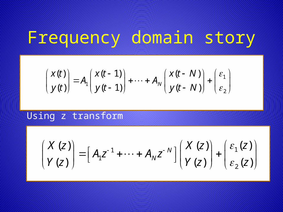
Frequency domain story
11
2
( ) ( 1) ( )
( ) ( 1) ( )N
x t x t x t NA A
y t y t y t N
Using z transform
111
2
( )( ) ( )
( ) ( ) ( )N
N
zX z X zA z A z
Y z Y z z

w
Z=exp(j )w
1 1
12 21
( ) ( )( ) 1( )
( ) ( ) ( )NN
z zX zH z
Y z z zI A z A z
1
2
( )( )( )
( ) ( )
XH
Y
11
22
1 1 1 2
2 1 2 2
212
221
( ) ( ) ( ) ( )( ) ( ) ( ) ( )( ) ( )
( ) ( ) ( ) ( )( ) ( ) ( ) ( )
( ) ( )xx xy
xy yy
X X X YH H
Y X Y Y
S SH H
S S
Where Sxx, is called autospectrum, Sxy cross-spectrum

w
In particular when s12=0,
11 22
11
2 2
2( ) log
xx xx xx xy xy
xxy x
xx xx
S H H H H
Sf
H H
w1
( )2y x y xF f d
Kolmogrov indentity

For general case
• Multyply both side of the noise vector a matrix, so that it becomes independent.
• The remaining part is identical

Guo SX, Wu J.F.H., Ding MZ, Feng J.F.(2008) Uncovering interactions in the frequence domain PLoS Comput Biol 4(5): e1000087. doi:10.1371/journal.pcbi.1000087

Causality between different frequencies


Exam. (seminar 3) 1. Assume that we have microarray data of a single gene activity x(t) for six
days , measured at day 1, 2,3,4,5 and 6, i.e. x(1) x(2) x(3) x(4) x(6) 1 2 -4 1 3We want to fit the data using AR(1) model (the mean of x(t) is normalized to
zero), y(t+1)=ay(t)+eWhere a is a constant and e is the noise.a) Find the coefficient a (5 marks)b) Find the variance of e (5 marks)c) If we want to predict the activity of the gene at day 7, how can you do it?

Answera)a=[(x(1),x(2),x(3),x(4),x(5))*(x(2),x(3),x(4),x(5),x(
6))’]/ [(x(1),x(2),x(3),x(4),x(5))*(x(1),x(2),x(3),x(4),x(5))’]=-7/22
b) variance= [(x(2)-a*x(1))^2+ (x(3)-a*x(2))^2+ (x(4)-a*x(3))^2+ (x(5)-a*x(4))^2+ (x(6)-a*x(5))^2]/5
c) y(7)=ax(6).

For simultaneously recorded gene activities x(t) and y(t), assume that we can fit them using the following VAR(2) model
x(t+1)=a11 x(t)+a12x(t-1)+a14y(t-1)+e1
y(t+1)=b21 x(t)+b24y(t-1)+e2
a) Can you rewrite (x(t),y(t)) in VAR(1)?b) How to assess whether (x(t),y(t)) is stable
or not?c) Y(t) is a Granger causal of x(t) implies that
a14 is not zero. How can you quantify the Granger causality?

Answera) X(t)= A X(t-1)+BX(t-2)+e
b) X(t) is stable if the coefficient matrix above
c) x(t+1)=c11 x(t)+c12x(t-1)+e3
Fy->x=log(var(e3)/var(e1))
0)2(
)1(
0)1(
)( e
tX
tX
I
BA
tX
tX
1|0
|
I
BAeig