computational data, data structures and reasoning in science

Chapter 4: Computational Data, Data Structures and Reasoning in Science

How can computer scientists help scientists advance scientific models? Simple: play on computers' strengths, parry computers' weaknesses.

First the strengths side. Scientists were among the first to use computers, and they used them for number crunching. Even the word “computer” is an artifact of this. Before about the Second World War the term “computer” referred to an occupation. A “computer” was a person, generally a female mathematics major, who performed tedious calculations. The war itself spurred the development of automated computers in Germany, the United Kingdom and the United States. Afterwards a “computer” was such device.

Postwar “computers”, like today's computers, were thought to be1 faster, more accurate and tireless, unlike their prewar human counterparts. Being fast, accurate (hopefully!) and unable to bore makes computers ideal for doing simulations and exhaustive search. Both simulations and exhaustive search require the calculation of many similar computations, which human “computers” would find long, boring and tedious.

On the weaknesses side are computers' complete lack of “common sense”. One manifestation of this is “garbagein, garbageout”. Developers have to be careful to think about how to ensure all input is valid. Invalid input will probably result in invalid output.

Also, just because all inputed values are valid does not mean that the output will be valid. Internal bugs might miscalculate values, which would probably affect its outputs.

4.1 “To a kid with a hammer, everything is a nail”

We computer scientists are trained in the art of solving problems with computers. We study languages, data structures and algorithms towards this end. But, just because computers could solve a problem does not mean that it is the best way to solve a problem.

Analytical solutions, when they exists, are just better. They are more general. They may be easier to convince yourself (and others) of their correctness. (They may depend on other proofs but they probably do not require you to take the integrity of a compiler, operating system, and hardware on faith.)

How to get an analytical solution? If you have a system of equations, try integration! Maybe you can do it. Differential equations are often classified as either “ordinary” or “partial” depending on whether or not there is just one or more than one independent variable. For ordinary differential equations many techniques exist including Laplace transformations, ztransformations, perturbation expansions, and discrete time equations. Partial differential equations are, in general, more difficult to deal with. Separating their variables, however, can

1 I use the qualifier “were thought to be” because when was the last time you checked a calculation by hand? A noteworthy case where computers were wrong was uncovered by Thomas Nicely in October 1994. Nicely, a mathematics professor at the Lynchburg College, found a problem with Intel's Pentium floatingpoint unit that affected some divisions.

Copyright (c) 2008 by Joseph Phillips. All Rights Reserved.

often greatly simplify them. Please see Neil Gershenfeld “The Nature of Mathematical Modeling” or some other authoritative reference on mathematical and computer modeling.

4.2 Computational Data in Science

The most basic piece of knowledge to represent in a computer is one value, either numeric or conceptual. Perhaps the value is a measurement, perhaps it is some interesting derived value (e.g. a mean, median or mode). Perhaps it is our best guess at some constant, like the speed of light. Or, perhaps it is some calculated value that is not a fundamental constant but just the result of a computation.

Associated with almost any value (except perhaps integer counts) is some notion of precision. Scientists often assume a normal Gaussian distribution of measurements. Recording summaries of such measurements requires at least two numbers: a mean and a variance, standard deviation, or some equivalent measure of spread. In computer science, however, we often use just one number. Thus, using the standard double or float variable to store such data loses information. A solution to this is to represent both values in two variables, or perhaps to use an object oriented language to develop special classes that can hold a mean and deviation. These both require added effort on the programmer.

The same issue also occurs with conceptual data. The terms “car”, “Toyota”, “Toyota Prius” and “the car with vehicle identification number XXXXXXXXXXX” refer to increasingly more specific sets of objects.

Beyond just the value and its variance is its units (and implicitly, its dimensions). This knowledge is important to the tune of $125 millions dollars. In 1999 an investigation board concluded that NASA engineers did not convert between pounds, an English measure of rocket thrust, to newtons, a metric measure, in the Mars Climate Orbiter. It is believed that this basic error resulted in the lost of the $125 million dollar spacecraft.

There are at least two ways to associate units with a value: in the variable name or with a class that records the value and units together. The easiest solution is to denote the units of a variable in its name, for example:

double speedOfLightInMetersPerSec = 299792458;

This allows developers to check if calculations are properly conducted in an easier fashion. Consider the following four expressions:

speedOfLightInMetersPerSec * timeInSecondsspeedOfLightInMetersPerSec * timeInHoursspeedOfLightInMetersPerSec * SECONDS_PER_HOUR * timeInHoursspeedOfLightInMetersPerSec + timeInHours

In the first expression, “PerSec” intuitively cancels “Seconds” to yield a value in units “Meters”.


In the second expression, “PerSec” does not properly cancel “Hours”. In the third expression, “MetersPerSecs” multiplied by “SECONDS_PER_HOUR” yields “MetersPER_HOUR”. “MetersPER_HOUR” multiplied by “InHours” just yields “meters”. In the fourth expression it is not clear if any useful value will result from adding a “MetersPerSec” value with an “HOURS” one.

A problem with relying purely on variable naming conventions is that it relies on humans to detect errors. Object oriented languages allow us to define classes that store both values and units. Some languages, like C++, further allow us to overload common arithmetic operators to work our new classes. This allows us to convert values and check dimensions automatically in intuitivelyconstructed expressions. A cost, however, is that we check the units and dimensions at run time.

Associated with almost all values is some sense of domain: the legal sets of values that it make sense. There are actually several interrelating notions of domain. Range definition limits define the limitations that logically bracket values. Latitude measurements, for example, are logically defined to lie between 90 degrees and +90 degrees. Latitudes outside this range make no sense. A given system may be subject to stricter system extent limits because the system being measured is limited. For example, if we are noting where events happened along a 1meter long track then positions like “1.2 meters” obviously lie outside. Also, empirically we might find that even though the system being measured could (in principle) support the value, in practice it is not observed. I call these saturation limits. For example, from January 1973 to April 2008 the United States Geological Survey only recorded one earthquake magnitude 9 earthquake2. Thankfully, earthquakes do not appear to get much larger3. All three limits are related by system constraints: saturation ones must lie within system extent one, which in turn must lie within range definition ones.

Related to those system limitations are also ones related to the equipment doing the measuring. The equipment may be unable to detect some events because they are too weak. I call these detection limits. Sometimes some events are on the threshold of detectability such that we can detect some events and miss others. This happens with earthquakes of small magnitude. If we have a seismometer of sufficient sensitivity then we can detect small tremors. A quake of the same size far from a seismometers may, however, register a background noise. I call these reliability limits. All three limits are related by instrumental constraints: reliability limits must lie within detection ones, which in turn must lie insider system extent ones.

Lastly there are data constraints on the actual observed values we see. The observed range of values must lie within the system extent limits and with the system detect limits.

For measurements, and perhaps values derived from them, it might be good to encode

2 The 2004 December 26th earthquake severely affected many countries around the Indian Ocean.3 Geophysicists have theorybased reasons to believe that earthquakes much larger cannot happen

(discounting asteroid impacts, very large bombs, etc.), at least while the Earth's plates are configured as they currently are. Earthquake magnitude is proportional to the length of the fault that slips. There are not many faults much bigger than the __ fault, which completely ruptured along its entire length on 2004 December 26.


when and where the value comes. While our best models tell us that the speed of light should be constant for all observers at all times, this generally is not the case. Consider a count of the number of robins in the Chicago area in April of some particular year. We can easily encode this as an integer with units “number of robins”. We ought, however, to also specify what we mean by “Chicago area” and note that this count corresponds to April of some year.

When a measurement comes from a complex apparatus we ought to note that equipment too. Astronomy is a good example. Before chargecoupledevice (CCD) cameras became widespread astronomers used to use particular cameras and particular film. It is good to note both the camera and film because later on it find some kind of systematic error associated with either. Systematic errors can often be corrected for, but we must know to do so.

We should also be mindful of who made a particular measurement. If we know their background then we might be able to guess the Kuhnian paradigm that they operated under. This knowledge might help us interpret their observation in our current paradigms.

According to Simon Mitton, between 532 B.C. and 1064 A.D. Chinese astronomers recorded many “guest stars”. Contemporary astronomers now interpret these “guest stars” as novae, supernovae and comets. When comets are excluded Mitton counted 75 novae and supernovae. These records are extremely important because supernovae are so rare. We now no longer believe that “guest stars” are “temporary stars”, rather we reinterpret the ancient Chinese data as a record of stellar explosions spanning more than a thousand years.

Related to who obtained the value is why. We may know that the observer had a particular agenda. This agenda may color his or her judgment, either consciously or subconsciously. Knowing this may help us better interpret the data.

4.3 Data Sources

Nowadays scientific data comes from laboratories of one form or another, and these tend to be highly specialized. Astronomers, for example, get much of their data from observatories. High energy physicists get much of their data from particle accelerators.

Data now is often gathered from multiple laboratories. For example, when interesting stellar events occur observatories worldwide take turns observing it while it is in the sky overhead. As it passes over the horizon observational responsibility passes to observatories further west.

The Human Genome Project showcases the distributed nature of modern “big” science. According to the Human Genome Project Information website (http://www.ornl.gov/sci/techresources/Human_Genome/home.shtml), there were five primary human genome project sequencing sites within the United States and United Kingdom: the U.S.DOE Joint Genome Institute; Baylor College of Medicine Human Genome Sequencing Center; The Wellcome Trust Sanger Institute; Washington University School of Medicine Genome Sequencing Center; and Whitehead Institute/MIT Center for Genome Research.


http://www.ornl.gov/sci/techresources/Human_Genome/home.shtml

Besides these five labs were at least 15 other labs in China, France, Germany, Japan, the United States that participated in smaller roles.

4.4 Data Catalogs

Scientific data culled from multiple sources is often tabulated in large databases. The distributed nature of data collection gives us at least five issues to ponder: (1) what is (and is not) recorded, (2) the distributed nature of catalogs, (3) synonyms and terms in catalogs, (4) missing and error terms, and (5) catalog permanence.

Catalogs record often record data like events. Implicit in the database's design, however, is the data and events that are not recorded. Events are sometimes excluded because they are deemed “outofbounds” along one or more dimension. In our “robin count in the Chicago area in April” the dimensions are partially spatial ones, limiting itself to however we define the “Chicago area”. They are partially temporal ones too: in this case “April”.

Temporal limitations may not be that neatly defined. If the limiting factor is funding then data may be collected until the money runs out. This may result in seemingly arbitrary periods. We may stuck having to do the best with the data we have.

Besides space, time and money, data also may be excluded if they represent events that are too weak to reliably detect. An example is earthquake data. The United States Geological Survey (USGS) has an online catalog that lets people download records of earthquakes delimited by space and time (http://neic.usgs.gov/neis/epic/). This catalog should, however, not be understood as recording every earthquake in the world. For recent earthquakes the catalog may be complete for all “large” quakes worldwide (say Mw > 7). It probably has most reasonably large quakes (say Mw > 6). It has many smaller earthquakes too, but only if they occur near seismometers. It probably excludes many more.

Of course the USGS probably places seismometers close to where earthquakes are expected to occur (e.g. California's San Andreas fault). However, these regions are the intersections of where earthquakes occur and where humans perceive economic interest. For example, the many earthquakes occur at the bottom of the oceans. Few of the small ones affect people. The USGS (and other organizations) records some of larger ones but does not detect (or ignores) the majority of small ones.

A naive look at the USGS catalog would suggest that the majority of small earthquakes happen in Western Europe, where most of the really sensitive seismometers reside. We must be cognizant of the geological (or other) biases that help determine what gets recorded.

(As an aside, earthquake data also provides an interesting time/money study, with politics thrown in. Geophysicists regard the later period of the Cold War as a “golden age” of geophysics. For the United States and the Soviet Union the Partial Test Ban Treaty of 1963 pushed the testing of nuclear weapons underground. Thus, the United States could not rely on the gathering of isotopes from the air to guess the types of nuclear weapons the Soviets were testing. The solution that the Americans came up with was to develop a broad seismological network to “listen” to Soviet nuclear weapons' tests. Perhaps it was the geophysicists and seismologists who benefited the most; they obtained records of many earthquakes from equipment designed to spy on the Russians.)


http://neic.usgs.gov/neis/epic/

As mentioned before data often gathered from many places and gathered into catalogs. For example, several databases centralize bioinformatics data like DNA and protein sequences, and crystal structures. This, of course, relates to the computer science fields of distributed databases and networking. For purposes of this discussion let us assume that good database design methodology has been followed giving us online databases that are suitably redundantly stored and reliably available at any time.

When data is gathered from many sources inconsistencies may appear. Terms may be used inconsistently. Different “missing” or “error” value conventions may be followed. Databases also may be outofdate relative to each other. Further, when data from many databases is centralized at one master “clearing house” database a “least common denominator” format may be followed; some information may not make expressible in the centralized database's schema.

A particular problem is “What exactly is denoted by particular terms?” To computers terms are often denoted as strings of characters in ASCII or perhaps Unicode. What then does the term “robin” mean? In North America it probably means the American robin, “Turdus migratorius”. In Europe it probably means the European robin, “Erithacus rubecula”. In Australia it probably means one of the members of family Petroicidae, of which there are about 45 species in about 15 genera.

Left: Turdus migratorius, the American robinCenter: Erithacus rubecula, the European robin

Right: Petroica phoenicea, one of several Australasian robins

Thus what you denote when you write “robin” probably depends on who (and where) you are.The situation is made more complex by using other, more general terms. Consider just the

American robin (Turdus migratorius). This robin is a member of the thrush family. The thrush family is in the larger group of songbirds. And, of course, all songbirds are birds. The terms “thrush family bird”, “songbird” and “bird” may or may not mean American robin.

This is not a new problem in computer science. The effort to develop ontologies was meant to address it. Ontologies are useful, if they are used.


Missing values and errors in the data are an additional difficulty with using databases. Missing values are often encoded as sentinel values, for example using 1 for counts or the terms “n/a” or “null”. If a given databased was gathered from many sources then there may be more than sentinel value in use.

Rules meant to ensure the gathering data may have a perverse, unintentional effect. Clerks one system were required by the system to enter a telephone number for their customers. What to do when the customer refuses to provide one? The most common telephone number in the database was (111)1111111, and it was shared by many customers. Obviously we must be aware of such rules and the ramifications that they may have on the data.

Errors on databases are probably (in some ways) a smaller problem with computers then with humans. If we give computers the tools to check data's integrity then they can use them. At a pure data transmission and storage level there are parity bits and checksums. For security concerns there are public encryption and cryptographic nonces.

At a higher level we can use rules to check if data “make sense”. The problem with rules is that they probably are inflexible and are subject to our own preconceptions. The United States and the United Kingdom both launched satellites to monitor ozone depletion in the atmosphere. The Americans programmed their system to ignore data that appeared too low. Thus they missed the ozone “hole” that appeared over Antarctica. The British detected it too, but they did not have the same bias that caused them to ignore it.

This issue also is not a new one for dealing with databases. Please see an authoritative source on data mining subfield of data cleaning.

Lastly, there is the issue of the permanence of the data. The quest to store pack more data on smaller and cheaper media has made many forms of storage obsolete: punch card, various forms of magnetic tape, 8inch magnetic disk, 5¼inch magnetic disk, and 3½inch magnetic disk are just a few examples. We now have very large and very cheap (on a perbyte basis storage). How long before it becomes obsolete? Even if we keep the original equipment around, how long will the original media last?

Hopefully the organization in charge of maintaining the database has a backup policy. However, this depends on the organizations level of technological sophistication, and its available budget.

Related to this are issues with the data itself. Perhaps some much data is generated that the organization cannot afford to archive all of it but only keeps around data from the last N time periods. Perhaps the data is subject to privacy issues and their is a policy to destroy it after so long. We should be aware of these issues too.

4.5 Data Structures for Knowledge for Prediction

A basic task in science is using a model to compute what it predicts. This (mostly) deductive operation underpins not just confirmation of old data and prediction of new, but also induction and abduction to see how well potential modifications of the model do.


In computer science we have some data structures for computing with numbers, others for working with symbols, and some for mixing. We will survey some important ones below.

4.5.1. Computing with Numbers: Equations

The dominant knowledge structure for working with numbers is the equation. Equations are strong and powerful things. At their bests we can given them N1 knowns and compute any desired single unknown. There is also information in their structure. If some of the values are vectors or matrices then one “equation” may be a shorthand for several scalar equations.

Consider the iconic “F = ma”. It tells us force and acceleration are acting in the same direction, and that mass is a scalar value. (We should also implicitly or explicitly remember the domain of the values. For example, we do not believe that mass can be negative.)

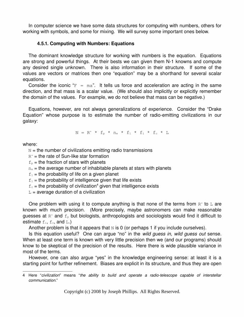
Equations, however, are not always generalizations of experience. Consider the “Drake Equation” whose purpose is to estimate the number of radioemitting civilizations in our galaxy:

N = R* * fp * ne * fl * fi * fc * L

where:N = the number of civilizations emitting radio transmissionsR* = the rate of Sunlike star formationfp = the fraction of stars with planetsne = the average number of inhabitable planets at stars with planetsfl = the probability of life on a given planetfi = the probability of intelligence given that life existsfc = the probability of civilization4 given that intelligence existsL = average duration of a civilization

One problem with using it to compute anything is that none of the terms from R* to L are known with much precision. (More precisely, maybe astronomers can make reasonable guesses at R* and fp but biologists, anthropologists and sociologists would find it difficult to estimate fi, fc, and L.)

Another problem is that it appears that N is 0 (or perhaps 1 if you include ourselves).Is this equation useful? One can argue “no” in the wild guess in, wild guess out sense.

When at least one term is known with very little precision then we (and our programs) should know to be skeptical of the precision of the results. Here there is wide plausible variance in most of the terms.

However, one can also argue “yes” in the knowledge engineering sense: at least it is a starting point for further refinement. Biases are explicit in its structure, and thus they are open

4 Here “civilization” means “the ability to build and operate a radiotelescope capable of interstellar communication.”


for discussion. For example, if we one day find life on the Jovian moon Europa or Saturn's moon Titan then perhaps it ought to be revised to allow for intelligence on moons too.

This is an important point. Equations (and other knowledge structures) can do more than just compute stuff. They also outline a rationale, a way of thinking, and especially at assumptions. The physicist Enrico Fermi was known for asking his students to estimate the number of piano tuners in a particular city on their tests. This was obviously not a question about quantum mechanics but an exercise to see how they broke problems down.

We can return to the classic “F = ma” and realize that this is not what Issac Newton wrote; instead he wrote (in modern Leibniz notation) “F = dp/dt” or “the force is equal to the change in momentum”. We can use calculus' Product Rule to obtain:

F = dp/dt= d(mv)/dt= m(dv/dt) + v(dm/dt)= ma + v(dm/dt)

Here p represents momentum, which is mass (m) times velocity (v). Differentiating the product mv yields a sum of two subexpressions. The term dv/dt (“the change in velocity with respect to time”) is just a, acceleration. The term dm/dt, however, is “the change in mass with respect to time”. Except for rockets, machine guns, conveyor belts and other things that expel or gain a nonnegligible amount of mass at large differences in velocity, the dm/dt term is usually 0, or close to it.

Thus, even our familiar “F = ma” is biased: it is appropriate for things that remain intact.

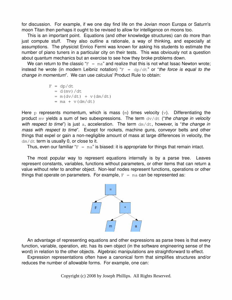
The most popular way to represent equations internally is by a parse tree. Leaves represent constants, variables, functions without parameters, or other items that can return a value without refer to another object. Nonleaf nodes represent functions, operations or other things that operate on parameters. For example, F = ma can be represented as:

An advantage of representing equations and other expressions as parse trees is that every function, variable, operation, etc. has its own object (in the software engineering sense of the word) in relation to the other objects. Algebraic manipulations are straightforward to effect.

Expression representations often have a canonical form that simplifies structures and/or reduces the number of allowable forms. For example, one can:


● remove subtraction operations and replace them with additions, where the expression being subtracted is multiplied by the constant -1,

● remove division operations and replace them with multiplications, where the divisor expression is raised to the power of the constant -1,

● arrange the terms of a polynomial equation such that the highest power is added first, the next highest second, etc., echoing how polynomials are commonly written.

4.5.2. Computing with Concepts: Rules, Decision Trees and Production Systems

Besides computing with numbers there is computing with concepts. This often entails computing one attribute from other attributes. Several techniques exist but the most common are rules, decision trees and production system.

Rules have an ifthen format for predicting one attribute's value given the the values of other attributes. For example the rule:

if dog(X) and wet(X) then smelly(X).

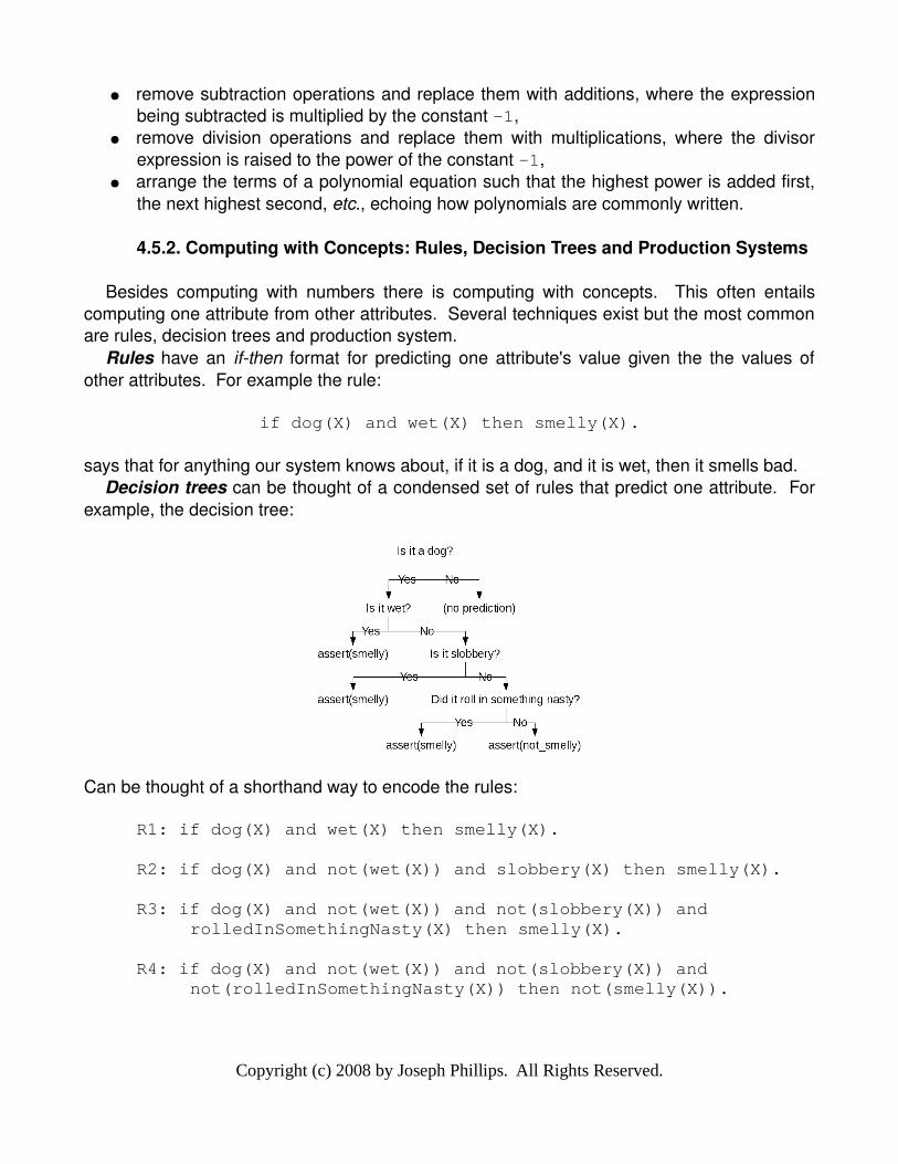
says that for anything our system knows about, if it is a dog, and it is wet, then it smells bad.Decision trees can be thought of a condensed set of rules that predict one attribute. For

example, the decision tree:

Can be thought of a shorthand way to encode the rules:

R1: if dog(X) and wet(X) then smelly(X).

R2: if dog(X) and not(wet(X)) and slobbery(X) then smelly(X).

R3: if dog(X) and not(wet(X)) and not(slobbery(X)) and rolledInSomethingNasty(X) then smelly(X).

R4: if dog(X) and not(wet(X)) and not(slobbery(X)) and not(rolledInSomethingNasty(X)) then not(smelly(X)).


Another way of computing with symbols is with production systems. Production systems are often used to implement knowledgebased (or “expert”) systems that try to encode domain expert knowledge about a particular subject. The productions themselves are ifthen rules but the production system architecture also includes a mechanism for keeping and revising the state that determines which rules will “fire”. We will see more concrete examples later.

As with equations there is also knowledge in the structure of rules and decision trees, and this is most clear with decision trees. Within the machine learning (ML) community of the artificial intelligence (AI) community there has been a decadeslong quest to develop ever better decision tree learning algorithms. ML folks generally define “better” to mean some quantification of “more accurate, subject to not overfitting”. Their heuristics often recursively compute which attribute offers the most discriminatory power in separating training examples into distinct sets that are as homogeneously labeled as possible.

This approach generally succeeds in finding reasonably accurate, reasonably generalized decision trees. However, the structures of these trees may or may not correspond to how domain experts arrange the data in their heads. (One example of this is the ML procedure of “boosting”: combining multiple “weak” classifiers with a weighted voting scheme into a better composite classifier than any individual “weak” classifier alone. It is not clear if individual scientists use weighted voting among contradictory models in their everyday reasoning.) Unlike a pure ML approach, computational scientific discoverers must take agreement with the form and content of prior knowledge into consideration.

4.5.3. Computing with Probabilistic Concepts: Bayesian Networks

Sometimes it is useful to model the Universe that is complex in the sense that there are many attributes that vary nondeterministically, but is simple in the sense that some attributes depend only on certain other attributes instead of the full state. (Equivalently, an attribute may depend on many other attributes, but we have only elucidated the relationships with a handful of more important or easier to explain attributes.)

Bayesian networks (also called “graphical models”) are useful is such cases. They represent patterns of nondeterministic influence with a graph: nodes represent attributes (or “variables” as they are known in Bayesian net community) and arcs between them represent the influence one variable has on another. Arcs may be directional or undirectional. Directional arcs represent influence that the “from” node has on the “to” node. Variables generally have a small and finitesized domain.

For the directional case each node has zero or more nodes coming into it. If it has zero then its variable depends on no other variable. The value it has depends on some a priori probability. Nodes with one or more arcs coming into them depend on the values that the incoming variables have. The value of the variable of interest is depends on a conditional probability of the incoming variables' values.

For example, imagine the following situation. You are in a class with a professor and a teaching associate (“ta”). Either one of the two may or may not assign homework (two boolean variables). You are interested in how busy you will be over the weekend (another


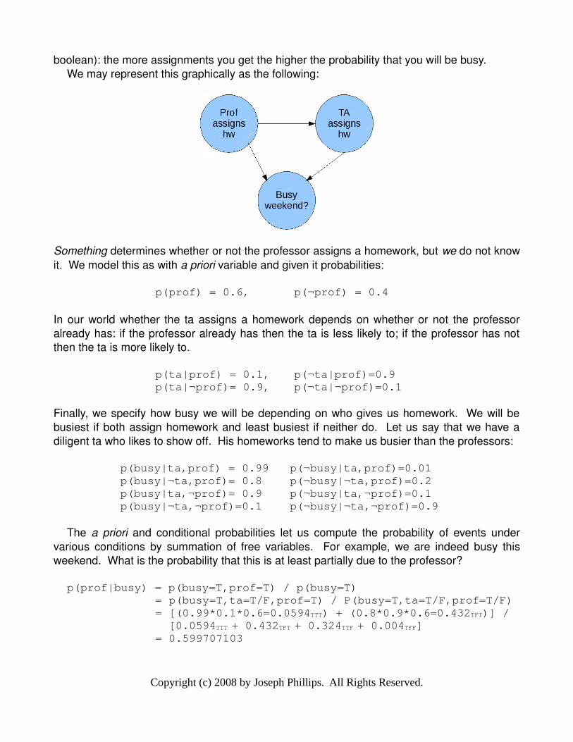
boolean): the more assignments you get the higher the probability that you will be busy.We may represent this graphically as the following:

Something determines whether or not the professor assigns a homework, but we do not know it. We model this as with a priori variable and given it probabilities:

p(prof) = 0.6, p(¬prof) = 0.4

In our world whether the ta assigns a homework depends on whether or not the professor already has: if the professor already has then the ta is less likely to; if the professor has not then the ta is more likely to.

p(ta|prof) = 0.1, p(¬ta|prof)=0.9p(ta|¬prof)= 0.9, p(¬ta|¬prof)=0.1

Finally, we specify how busy we will be depending on who gives us homework. We will be busiest if both assign homework and least busiest if neither do. Let us say that we have a diligent ta who likes to show off. His homeworks tend to make us busier than the professors:

p(busy|ta,prof) = 0.99 p(¬busy|ta,prof)=0.01p(busy|¬ta,prof)= 0.8 p(¬busy|¬ta,prof)=0.2p(busy|ta,¬prof)= 0.9 p(¬busy|ta,¬prof)=0.1p(busy|¬ta,¬prof)=0.1 p(¬busy|¬ta,¬prof)=0.9

The a priori and conditional probabilities let us compute the probability of events under various conditions by summation of free variables. For example, we are indeed busy this weekend. What is the probability that this is at least partially due to the professor?

p(prof|busy) = p(busy=T,prof=T) / p(busy=T)= p(busy=T,ta=T/F,prof=T) / P(busy=T,ta=T/F,prof=T/F)= [(0.99*0.1*0.6=0.0594TTT) + (0.8*0.9*0.6=0.432TFT)] / [0.0594TTT + 0.432TFT + 0.324TTF + 0.004TFF]= 0.599707103


4.6 Algorithms for Knowledge for Prediction

Computers, as was mentioned at the beginning of the chapter, are most helpful when the are called upon to do tasks with multiple repetitive calculations, like simulations and exhaustive search. We will discuss exhaustive search in the next chapter and touch on prediction techniques below.

Our discussion of prediction techniques will proceed from numeric to symbolic, starting with numeric simulation.

4.6.1 Numeric Simulation

The topic of simulation by computer is are large one. I offer a very brief overview below and refer you to books like Ingels' (What Every Engineer Should Know About) Computer Modeling and Simulation and Gershenfeld's The Nature of Mathematical Modeling for more detail.

Computer simulation is a broad topic because some many different types of simulation may be done. Simulations may be:

1. Deterministic or stochastic2. Discrete or continuous3. Static or dynamic4. Linear or nonlinear5. Batch, realtime, or something else

Whatever the type of simulation they ought to be undertaken like any good software engineering effort. There are often four steps:

1. Going from the real system to some logical abstraction of it,2. Choosing the appropriate data structures, algorithms and (when applicable) numerical

techniques,3. Implementing the technique as a program, and4. Validating the program.

In what follows we will touch on topics 1, 2 and 4 because they are covered in other computer science, software engineering and numerical methods books and references. Topic 3, however, warrants its own section because some implementation languages may not be well known to computer scientists.

The most important thing when going from the real system to some abstraction of it is to define what the goals are for the project. What questions do the scientists want answered? What might they reasonably want a few years in the future?

Defining the goals is crucial because it can help you with the next task: deciding what to include in the model and exclude from the model. When in doubt, leave it out. Model can always be modified to be more complex in the future if they lack some crucial detail. However, if the model starts out complex, and the scientists are unhappy with it, what should one do? Is it that some detail already in the model is wrong? Or is it that the model is


missing some detail? Or is it both? Start simply.Spend time defining the goals as best you can because they are needed to determine

whether or not the effort succeeded, failed, or was a partial success. In particular, they are needed for validation. Revisit them as the project progresses. This mirrors modern software engineering practices.

The second issue for doing computer simulation is finding the appropriate data structures, algorithms and numerical techniques. Again the advice here is pretty standard in software engineering and modeling in general:

● Start with what's known● Go from simple to increasingly more complex● Iterate● Develop large models modularly● Model only what is necessary● Make (and state) assumptions and hypotheses● State constraints● Alternate between topdown & bottom up approaches

For advice on the actual mechanics of choosing the best algorithm or data structure I refer you to a book on data structures and algorithms, such as Cormen et al's Introduction to Algorithms. For advice on choosing the best numerical technique I refer you to books on those topics, such as Gershenfeld's The Nature of Mathematical Modeling and Press et al's Numerical Recipes 3rd Edition: The Art of Scientific Computing.

Validation is the fourth issue. Because simulations are so complex and difficult to check by hand it is important that someone define some test cases to check the software. This should be done early in the design phase so everyone is clear about what “success” looks like.

Someone has to come up with the test cases. Ideally that person is a scientists his or her self. After all, they are the client and domain expert; they should know best what good results look like. Cases may also come from other trusted sources, like wellregarded textbooks, papers or reputable websites. If none of these sources is available a computer scientists should try to define some cases his or herself, by hand (or perhaps easilychecked program) and then have them checked by a domain expert. Again, this is just good software engineering practice.

Developers can have a wide range of programming approaches to implement modeling. Here I will touch on five general classes: procedural languages, object oriented languages, artificial intelligence languages, production systems, and simulation languages. Production systems can be considered artificial intelligence languages but we will discuss them separately. QSIM, a language for qualitative simulations, will have its own subchapter after this one.

Procedural programming languages (or imperative programming languages) are noted for their explicit list of instructions telling the computer what to do. Among these instructions are


loops, conditionals, and calls to subroutines (other lists of instructions). They have a long tradition in computer science; assembly language is itself a very lowlevel procedural langauge. Fortran (“FORmula TRANslation”) among the first highlevel languages ever developed, was designed for the purpose of coding scientific applications. Experience with Fortran, Cobol and other firstgeneration high level programming languages lead to a computational theory of computers languages and the development of Algol in the 1960s. Algol was very important language because it influenced most other languages that came after it including Pascal and C. C, a relatively “lowlevel” highlevel language, has had its development intertwined with that of the Unix operating system.

Procedural languages are fast. People have been thinking about optimization in Fortran compilers for 50 about years. C has been called a “portable assembly language” and is easier to design decent compilers for than more complex languages (like Ada). Procedural languages also have large libraries of scientific applications and routines that may be used, minimizing the need to “reinvent the wheel.”

Despite these advantages procedural languages have been falling out of favor for most applications since the mid 1990s. Procedural languages require that the developer to map the domain into primitive computer language elements with little help from the language itself.

Object oriented languages are noted for their ability to let the programmer define hierarchical classes corresponding to domain objects. Inheritance among classes serves to reduce the effort to develop any one particular class, and to encapsulate data structures to create abstract data types. They began with the simulation language Simula67 in the 1960s and Xerox PARC language Smalltalk in the early 1970s. Modula2, a programming language widely used in Europe in the 1980s, popularized the notion of module programming. Ada served the same role in the United States. In the early 1980s a new generation of true objectoriented languages were developed which included C++, Eiffel and Objective C. In the late 1980s and early 1990s C++ became popular in the United States. This was due in part to its syntactical similarity to C, with which American programmers were already familiar. By the mid 1990s some problems with C++ were cleaned up by the Sun Computer company with Java. Later, Microsoft also cleaned up C++ to define C#, a language closer to C++ but with a memory management policy highly influenced by Java. In the first decade of the 21st century both Java and C# are popular programming languages.

Object oriented languages are good for programming scientific applications in the same sense that they are for programming other applications: they encourage the programmer to develop a way to think in the problem domain space instead of the computer language element space. Classes can naturally correspond to scientific objects. Methods for those classes can naturally correspond to transitions that the scientific objects are may undergo. Further, languages like C++ can easily link into the large body of scientific code written in C.

Programming scientific applications in object oriented languages is often easier than in procedural languages, but the programmer must still develop the classes and methods. The languages generally do not natively support scientific concepts or transformations.

Artificial intelligence languages are used by AI researchers to develop AI applications. AI


applications are designed to help programmers implement problem solving techniques. There are several languages but I will discuss Prolog and Lisp below because they represent two different approaches.

Prolog was developed in France and Scotland in the 1970s as a way to do logic programming. It is limited to use Horn clauses, logic sentences that either may be thought of as a disjunction where all but one term has been negated:

NOT(a) OR NOT(b) OR NOT(c) OR z.

or as an implication where the condition is a conjunction of nonnegated terms and the “then” result is a single nonnegated term:

If a AND b AND c THEN z.

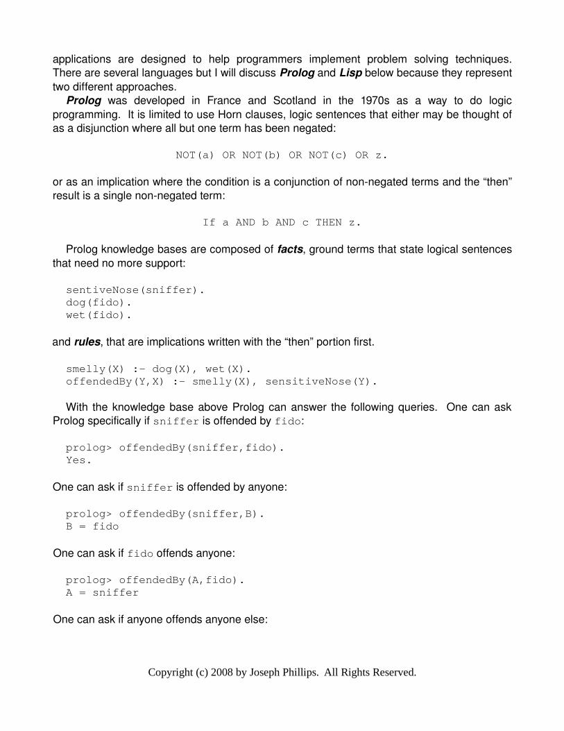
Prolog knowledge bases are composed of facts, ground terms that state logical sentences that need no more support:

sentiveNose(sniffer).dog(fido).wet(fido).

and rules, that are implications written with the “then” portion first.

smelly(X) :- dog(X), wet(X).offendedBy(Y,X) :- smelly(X), sensitiveNose(Y).

With the knowledge base above Prolog can answer the following queries. One can ask Prolog specifically if sniffer is offended by fido:

prolog> offendedBy(sniffer,fido).Yes.

One can ask if sniffer is offended by anyone:

prolog> offendedBy(sniffer,B).B = fido

One can ask if fido offends anyone:

prolog> offendedBy(A,fido).A = sniffer

One can ask if anyone offends anyone else:


prolog> offendedBy(A,B).A = sniffer,B = fido

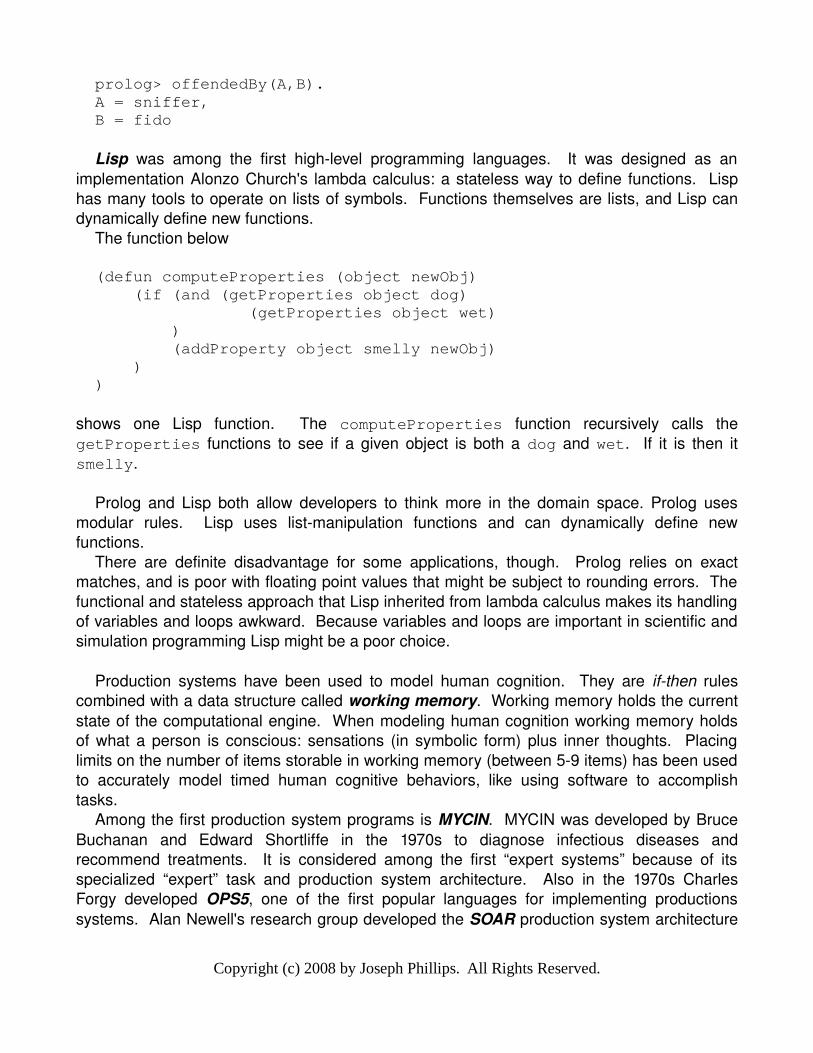
Lisp was among the first highlevel programming languages. It was designed as an implementation Alonzo Church's lambda calculus: a stateless way to define functions. Lisp has many tools to operate on lists of symbols. Functions themselves are lists, and Lisp can dynamically define new functions.

The function below

(defun computeProperties (object newObj) (if (and (getProperties object dog) (getProperties object wet) ) (addProperty object smelly newObj) ))

shows one Lisp function. The computeProperties function recursively calls the getProperties functions to see if a given object is both a dog and wet. If it is then it smelly.

Prolog and Lisp both allow developers to think more in the domain space. Prolog uses modular rules. Lisp uses listmanipulation functions and can dynamically define new functions.

There are definite disadvantage for some applications, though. Prolog relies on exact matches, and is poor with floating point values that might be subject to rounding errors. The functional and stateless approach that Lisp inherited from lambda calculus makes its handling of variables and loops awkward. Because variables and loops are important in scientific and simulation programming Lisp might be a poor choice.

Production systems have been used to model human cognition. They are ifthen rules combined with a data structure called working memory. Working memory holds the current state of the computational engine. When modeling human cognition working memory holds of what a person is conscious: sensations (in symbolic form) plus inner thoughts. Placing limits on the number of items storable in working memory (between 59 items) has been used to accurately model timed human cognitive behaviors, like using software to accomplish tasks.

Among the first production system programs is MYCIN. MYCIN was developed by Bruce Buchanan and Edward Shortliffe in the 1970s to diagnose infectious diseases and recommend treatments. It is considered among the first “expert systems” because of its specialized “expert” task and production system architecture. Also in the 1970s Charles Forgy developed OPS5, one of the first popular languages for implementing productions systems. Alan Newell's research group developed the SOAR production system architecture


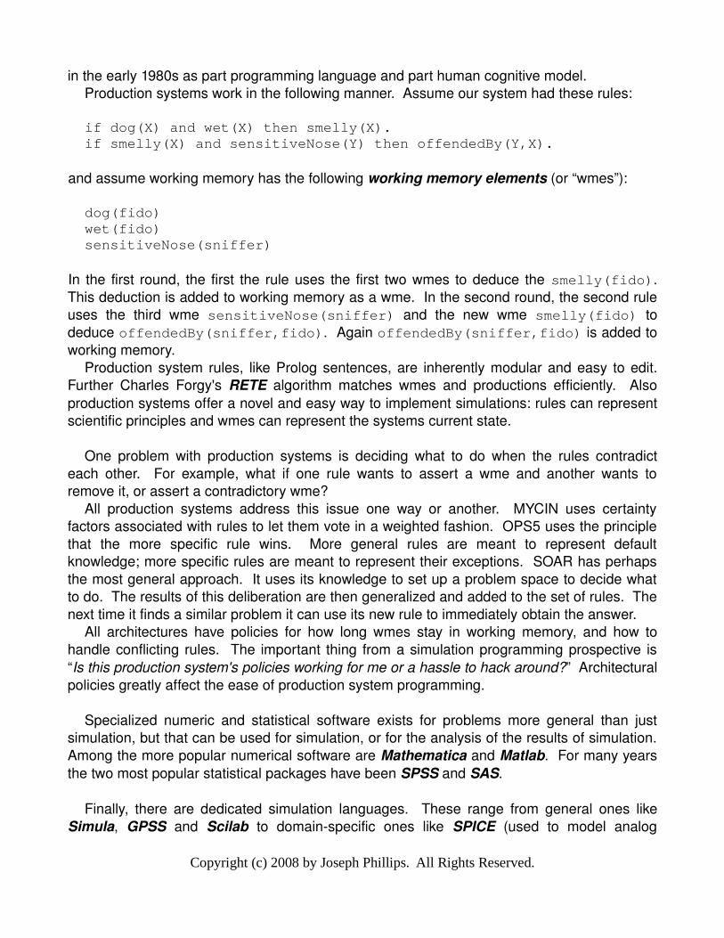
in the early 1980s as part programming language and part human cognitive model.Production systems work in the following manner. Assume our system had these rules:

if dog(X) and wet(X) then smelly(X).if smelly(X) and sensitiveNose(Y) then offendedBy(Y,X).

and assume working memory has the following working memory elements (or “wmes”):

dog(fido)wet(fido)sensitiveNose(sniffer)

In the first round, the first the rule uses the first two wmes to deduce the smelly(fido). This deduction is added to working memory as a wme. In the second round, the second rule uses the third wme sensitiveNose(sniffer) and the new wme smelly(fido) to deduce offendedBy(sniffer,fido). Again offendedBy(sniffer,fido) is added to working memory.

Production system rules, like Prolog sentences, are inherently modular and easy to edit. Further Charles Forgy's RETE algorithm matches wmes and productions efficiently. Also production systems offer a novel and easy way to implement simulations: rules can represent scientific principles and wmes can represent the systems current state.

One problem with production systems is deciding what to do when the rules contradict each other. For example, what if one rule wants to assert a wme and another wants to remove it, or assert a contradictory wme?

All production systems address this issue one way or another. MYCIN uses certainty factors associated with rules to let them vote in a weighted fashion. OPS5 uses the principle that the more specific rule wins. More general rules are meant to represent default knowledge; more specific rules are meant to represent their exceptions. SOAR has perhaps the most general approach. It uses its knowledge to set up a problem space to decide what to do. The results of this deliberation are then generalized and added to the set of rules. The next time it finds a similar problem it can use its new rule to immediately obtain the answer.

All architectures have policies for how long wmes stay in working memory, and how to handle conflicting rules. The important thing from a simulation programming prospective is “Is this production system's policies working for me or a hassle to hack around?” Architectural policies greatly affect the ease of production system programming.

Specialized numeric and statistical software exists for problems more general than just simulation, but that can be used for simulation, or for the analysis of the results of simulation. Among the more popular numerical software are Mathematica and Matlab. For many years the two most popular statistical packages have been SPSS and SAS.

Finally, there are dedicated simulation languages. These range from general ones like Simula, GPSS and Scilab to domainspecific ones like SPICE (used to model analog


circuits). There are several such languages and programming environments. Rather than give an overview of them I will discuss one designed for unique scientific applications: QSIM, a qualitative reasoning language.

4.6.2 Computer Algebra Systems

Before slavishly plugging numbers in to a set of equations it is useful to ask for a simplification. An algorithmic argument for this is that a simpler set of expressions might be easier to compute. A knowledgeunderstanding reason for this is that you may find an analytical solution. Recall: analytical solutions are the coolest and most general. They might lead to deeper insights into your domain.

A computer algebra system (or CAS) is used for algebraic manipulation, including simplifications, integrations, etc. They are useful in domains where there are many interrelated equations, like physics and engineering. Examples include Mathematica and Maple. While Mathematica also has numerical calculation ability too, in general CAS just do algebraic manipulation. They should be distinguished from numerical software (like Matlab) and statistical packages (like SAS and SPSS).

4.6.3 Probabilistic Reasoning and Bayesian Networks

We have discussed calculation of probabilities in Bayesian nets by summation over nonfixed variables, but this does not use the full power of the networks. It would be annoying to do if the network was large, but oftentimes we may use the geometry of the network to simplify the calculation.

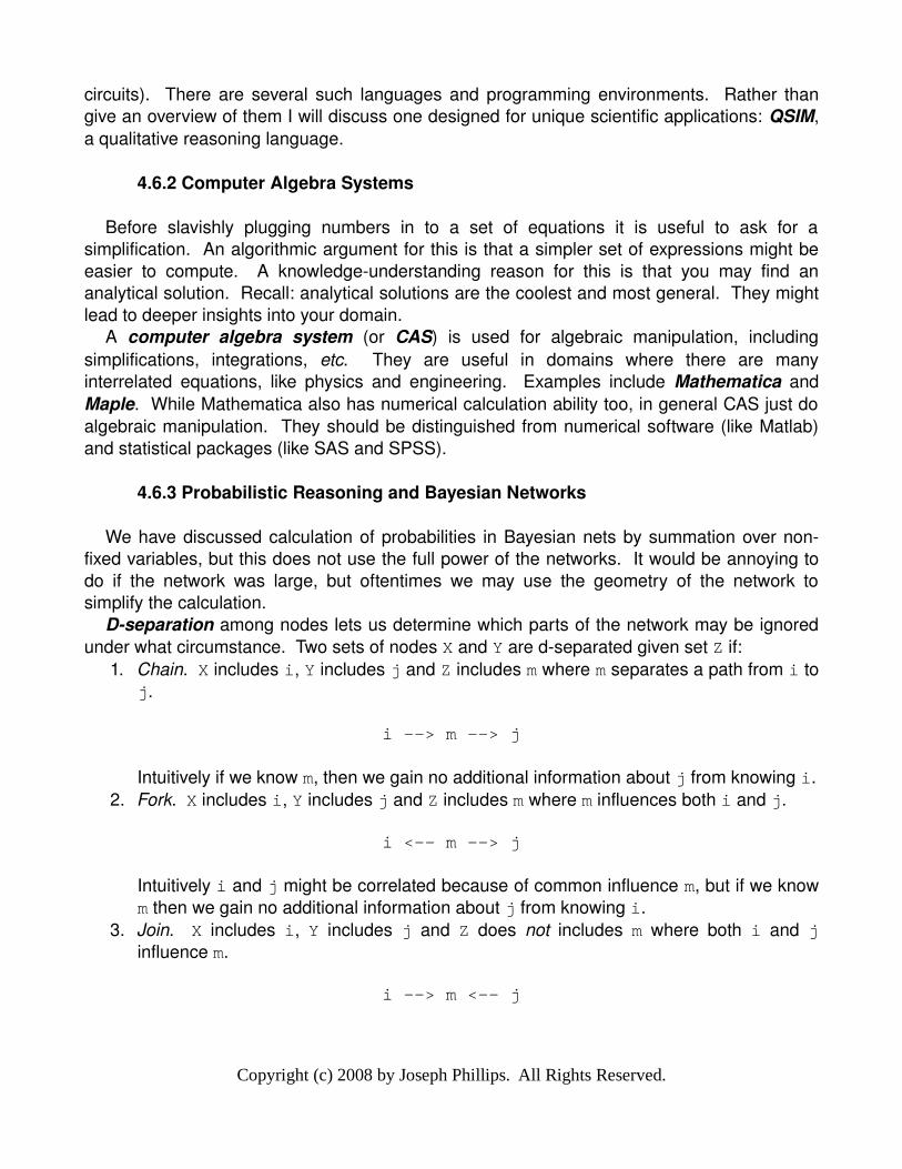
Dseparation among nodes lets us determine which parts of the network may be ignored under what circumstance. Two sets of nodes X and Y are dseparated given set Z if:

1. Chain. X includes i, Y includes j and Z includes m where m separates a path from i to j.

i --> m --> j

Intuitively if we know m, then we gain no additional information about j from knowing i.2. Fork. X includes i, Y includes j and Z includes m where m influences both i and j.

i <-- m --> j

Intuitively i and j might be correlated because of common influence m, but if we know m then we gain no additional information about j from knowing i.

3. Join. X includes i, Y includes j and Z does not includes m where both i and j influence m.

i --> m <-- j


Intuitively because both i and j influence m, if we knew i and we knew m then i's influence on m could suffice to explain it. Variable j would be less likely to have an isupporting value. For example, let i be “the floor is slippery”, let j be “the floor has a small bump” and let m be “someone fell”. If we knew that someone fell and that the floor was slippery then we would feel less inclined to posit a bump in the floor; the floor's slipperiness already has that explanatory capacity.

Algorithms for computation with Bayesian networks is a topic of ongoing research. Please see ___.

4.6.4 Qualitative Reasoning and QSIM

Qualitative reasoning was an area of active research in AI in the 1980s and early 1990s. The idea behind it is to model a physical system as well as possible given very little numeric information. Instead, the behavior of systems was to be modeled qualitatively. States described qualitatively would yield new states in the future. When insufficient knowledge was available to predict just one successor state, multiple possible successors would be given.

The following example from Kuipers gave a taste of their approach. If one wanted to model how something falls one could use highly specific numeric knowledge and data, for example:

d2x/dt2(t) = -9.8 m/sec2

v(t0) = 0 m/secx(t0) = 2 m

Abstracting away the specific numbers gives us a more general solution, at the expense of leaving some detail:

d2x/dt2(t) = -gv(t0) = v0

x(t0) = x0

This more general form uses lets the user specify the gravitational acceleration constant as well as the initial velocity and position. This lets us apply the model in more general circumstances than just 2 meters above the surface of the Earth.

The qualitative reasoning folks take this one step further. They ignore d2x/dt2(t) altogether except to note that dx/dt becomes smaller with time. For x(t) they only note when it is above the surface ([0..infinity]) or at the surface (0).

It what follows I describe the QSIM approach to qualitative reasoning by Kuipers. There are other similar methodologies though. de Kleer and Brown introduced confluences as an alternative representation of qualitative differential equations. Ken Forbus presented Qualitative Process Theory as an alternative, compatible approach. Lastly, B. C. Williams developed Temporal Constraint Propagation as another alternative.

QSIM and other approaches define variables. Variables have values but these values are


limited to represent only landmark values (e.g. MAX_CAPACITY) or the constants 0, -infinity or +infinity. Values may also take on ranges between landmark values, like capacity = (0..MAX_CAPACITY) and time = (t0,t1).

Besides a value, variables also have a derivative. Derivatives are also qualitative: either increasing (inc), decreasing (dec) or steady (std).

QSIM functions are very simple: they are either monotonically increasing (M+) or monotonically decreasing (M-).

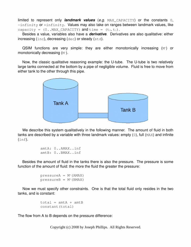
Now, the classic qualitative reasoning example: the Utube. The Utube is two relatively large tanks connected at the bottom by a pipe of negligible volume. Fluid is free to move from either tank to the other through this pipe.

We describe this system qualitatively in the following manner. The amount of fluid in both tanks are described by a variable with three landmark values: empty (0), full (MAX) and infinite (inf).

amtA: 0..AMAX..infamtB: 0..BMAX..inf

Besides the amount of fluid in the tanks there is also the pressure. The pressure is some function of the amount of fluid: the more the fluid the greater the pressure:

pressureA = M+(AMAX)pressureB = M+(BMAX)

Now we must specify other constraints. One is that the total fluid only resides in the two tanks, and is constant:

total = amtA + amtBconstant(total)

The flow from A to B depends on the pressure difference:


pAB = pressureA - pressureBflowAB = M+(pAB)d(amtA)/dt = flowABd(amtB)/dt = -flowAB

We also need knowledge about the domains of the variables:

total: 0..infamtA: 0..AMAX..inf amtB: 0..BMAX..infpressureA: 0..inf pressureB: 0..infpAB: -inf..0..infflowAB: -inf..0..inf

Finally, we need correspondences: statements that one variable will be at a landmark value when and only when another variable is at one of its landmark values:

c1: pressureA & amtA: (0,0), (inf,inf)c2: pressureB & amtB: (0,0), (inf,inf)c3: flowAB & pAB: (-inf, -inf), (0,0), (inf,inf)

We are done! Note the correspondence between qualitative and numeric qualitative equations:

d(amtB)/dt = f(g(amtA) � h(amtB))

where f, g and h are all in the set of M+.

We represent states by giving variables and their derivatives. Imagine filling tank A. (Ignore tank B, imagine the pipe has been closed.) At time t0 the tank is empty, but being filled: amtA = <0,inc>. The next state is a range between two landmarks: empty (t0) and full (t1). We represent this state as (t0,t1). During this state tank A is partially full but still being filled: amtA = <(0,AMAX),inc>. Finally the tank is full at time t1 so we stop filling it. We represent this as amtA = <AMAX,std>.

Now we let us try to predict the Utube's behavior. Imagine that at time t0 tank A is full and tank B is empty:

amtA = <AMAX,?>amtB = <0,?>

The first thing to do is determine the values (and derivatives) of the variables using the correspondences.

amtB = 0 therefore by c2: pressureB = 0


amtA = AMAX therefore by c1: pressureA = (0,inf)

amtA = AMAX && amtB = 0therefore by total's defining sum:total = (0,inf)

pressureA = (0,inf) and pressureB = 0 therefore by pAB's defining difference:

pAB = (0,inf)

constant(total) therefore by the definition of “constant” d(total)/dt = std

pAB = (0,inf) therefore by c3: flowAB = (0,inf)

flowAB = (0,inf) therefore by the definitions of the two derivatives:d(amtA)/dt = decd(amtB)/dt = inc

d(amtA)/dt = dec therefore by c1 again: d(pressureA)/dt = dec.

d(amtB)/dt = dec therefore by c2 again: d(pressureB)/dt = dec.

With the additional constraint (c4) that if d(pressureA)/dt = dec and d(pressureB)/dt = inc then d(pAB)/dt = dec we can propagate our last value:

d(pAB)/dt = dec therefore by c3 and c4: d(flowAB)/dt = dec

That was a lot of work, but now we have fully qualitatively specified the system at time t0:

amtA = <AMAX,dec> pressureA = <(0,inf),dec>amtB = <0,inc> pressureB = <0,inc>pAB = <(0,inf), dec> flowAB = <(0,inf), dec>total = <(0,inf), std>

The next thing to do is to predict the next state. The next qualitative state occurs when either:

1. A variable reaches a landmark value, or2. A variable leaves a landmark value, or3. A variable stops are starts moving

In this case there are 6 variables (not counting total, which is constant), each of which may do four things (options 1, 2 or 3 above, or not change). This gives us an upper limit of 461 = 4095 different states, but the correspondences and other constraints will reduce this considerably.


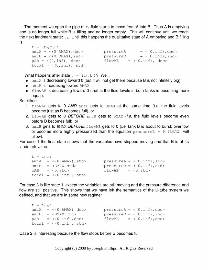
The moment we open the pipe at t0 fluid starts to move from A into B. Thus A is emptying and is no longer full while B is filling and no longer empty. This will continue until we reach the next landmark state: t1. Until this happens the qualitative state of A emptying and B filling is:

t = (t0,t1):amtA = <(0,AMAX),dec> pressureA = <(0,inf),dec>amtB = <(0,BMAX),inc> pressureB = <(0,inf),inc>pAB = <(0,inf), dec> flowAB = <(0,inf), dec>total = <(0,inf), std>

What happens after state t = (t0,t1)? Well:● amtA is decreasing toward 0 (but it will not get there because B is not infinitely big)● amtB is increasing toward BMAX.● flowAB is decreasing toward 0 (that is the fluid levels in both tanks is becoming more

equal).So either:

1. flowAB gets to 0 AND amtB gets to BMAX at the same time (i.e. the fluid levels become just as B becomes full), or

2. flowAB gets to 0 BEFORE amtB gets to BMAX (i.e. the fluid levels become even before B becomes full), or

3. amtB gets to BMAX BEFORE flowAB gets to 0 (i.e. tank B is about to burst, overflow or become more highly pressurized than the equation pressureB = M+(BMAX) will allow).

For case 1 the final state shows that the variables have stopped moving and that B is at its landmark value:

t = t1(a):amtA = <(0,AMAX),std> pressureA = <(0,inf),std>amtB = <BMAX,std> pressureB = <(0,inf),std>pAB = <0,std> flowAB = <0,std>total = <(0,inf), std>

For case 3 is like state 1, except the variables are still moving and the pressure difference and flow are still positive. This shows that we have left the semantics of the Utube system we defined, and that we are in some new regime:

t = t1(c):amtA = <(0,AMAX),dec> pressureA = <(0,inf),dec>amtB = <BMAX,inc> pressureB = <(0,inf),inc>pAB = <(0,inf),dec> flowAB = <(0,inf),dec>total = <(0,inf), std>

Case 2 is interesting because the flow stops before B becomes full.


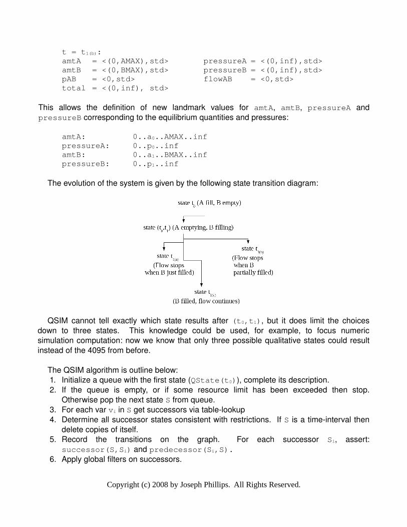
t = t1(b):amtA = <(0,AMAX),std> pressureA = <(0,inf),std>amtB = <(0,BMAX),std> pressureB = <(0,inf),std>pAB = <0,std> flowAB = <0,std>total = <(0,inf), std>

This allows the definition of new landmark values for amtA, amtB, pressureA and pressureB corresponding to the equilibrium quantities and pressures:

amtA: 0..a0..AMAX..infpressureA: 0..p0..infamtB: 0..a1..BMAX..infpressureB: 0..p1..inf

The evolution of the system is given by the following state transition diagram:

QSIM cannot tell exactly which state results after (t0,t1), but it does limit the choices down to three states. This knowledge could be used, for example, to focus numeric simulation computation: now we know that only three possible qualitative states could result instead of the 4095 from before.

The QSIM algorithm is outline below:1. Initialize a queue with the first state (QState(t0)), complete its description.2. If the queue is empty, or if some resource limit has been exceeded then stop.

Otherwise pop the next state S from queue.3. For each var vi in S get successors via tablelookup4. Determine all successor states consistent with restrictions. If S is a timeinterval then

delete copies of itself.5. Record the transitions on the graph. For each successor Si, assert:

successor(S,Si) and predecessor(Si,S).6. Apply global filters on successors.


7. Add successors to queue. Don't add inconsistent state, quiescent states, cycles, transition or t = inf states.

8. Go to 2

4.7 Summary

This chapter has explored issues related to data, knowledge and algorithms appropriate for scientific representation and reasoning. In the next chapter we will discuss machine learning principles for creating new knowledge, and how to modify them for scientific discovery.

References:Buchanan, Bruce G.; Shortliffe, Edward H. “RuleBased Expert Systems: The MYCIN

Experiments of the Stanford Heuristic Programming Project” AddisonWesley. USA. 1985.Cable News Network. “NASA: Human error caused loss of Mars orbiter.”

http://www.cnn.com/TECH/space/9911/10/orbiter.02/. November 10, 1999.Cormen, Thomas H., Leiserson, Charles E., Rivest, Ronald L., Stein, Clifford. “Introduction to

Algorithms, Second Edition”. McGraw Hill/MIT Press. Cambridge, Massachusetts. 2001.de Kleer, J.; Brown, J. S. “A qualitative physics based on confluences.” Artificial Intelligence.

24: 783. 1984. Also in Brachman and Levesque (ed.) Reading in Knowledge Representation. p. 88126. Morgan Kaufmann. 1985.

Emery, Vince. “The Pentium Chip Story: A Learning Experience” http://www.emery.com/bizstuff/nicely.htm. 1996.

Forbus, Ken D. “Qualitative process theory”. Artificial Intelligence. 24:85168. 1984.Forgy, Charles. "Rete: A Fast Algorithm for the Many Pattern/Many Object Pattern Match

Problem", Artificial Intelligence, 19, pp 1737, 1982Gershenfeld, Neil. “The Nature of Mathematical Modeling”. Cambridge University Press.

Cambridge, United Kingdom. 1999.Ingels, Don M. “(What Every Engineer Should Know About) Computer Modeling and

Simulation.” Marcel Dekker Inc. New York. 1985.Jaschek, Carlos. “Data in Astronomy” Cambridge University Press. Cambridge, Great

Britain. 1989.Kuipers, Benjamin. “Qualitative Reasoning: Modeling and Simulation with Incomplete

Knowledge” The Massachusetts Institute of Technology Press. Cambridge, Massachusetts. 1994.

Mitton, Simon. “The Crab Nebula”. Charles Scribner's Sons, New York. 1978.Morton, Oliver. “A Mirror in the Sky: The Drake Equation” in Farmelo, Graham (ed.) It Must

Be Beautiful: Great Equations of Modern Science. p. 4667. Granta Books. New York. 2003.

Newell, Alan. Unified Theories of Cognition, Harvard University Press. Cambridge, Massachusetts. 1994.

Press, William H., Teukolsky, Saul A., Vetterling, William T., Flannery, Brian P. “Numerical Recipes, Third Edition: The Art of Scientific Computing” Cambridge University Press. Cambridge, United Kingdom. 2007.


http://www.seds.org/messier/m-ref.html#mitton

http://en.wikipedia.org/wiki/Artificial_Intelligence_(journal)

http://www.cnn.com/TECH/space/9911/10/orbiter.02/

United States Department of Energy Office of Science, “Human Genome Research Sites”, http://www.ornl.gov/sci/techresources/Human_Genome/home.shtml. February 20, 2008.

Williams, B. C. “Qualitative analysis of MOS circuits” Artificial Intelligence. 24:281346, 1984.Williams, B. C. “Doing time: Putting qualitative reasoning on firmer ground.” In Proceeding of

the 5th National Conference on Artificial Intelligence. p. 105112. San Mateo, CA. Morgan Kaufman. 1986.












computational data, data structures and reasoning in science

Documents