computational finance – portfolio optimization and capital allocation

7/27/2019 Computational Finance – Portfolio Optimization and Capital Allocation

http://slidepdf.com/reader/full/computational-finance-portfolio-optimization-and-capital-allocation 1/13

1 Introduction 1

Computational Finance – PortfolioOptimization and Capital Allocation

1 Introduction

Given a set of n instruments s1, . . . , sn with with possibly uncertain returns, the task is toselect a portfolio θ1, . . . , θn of the instruments so as to maximize one’s utility.

More formally, let p1, . . . , pn be the current prices of the instruments, and let the futureprices be q 1, . . . , q n. The future prices q i are random variables. There may be a risk freeasset s0 with current price p0 and deterministic future price q 0. Let W 0 be the wealth now,available to be invested, and assume that a fraction of this wealth wi is invested in instrumenti, so that the number of units θi of each instrument purchased is given by

θi =wiW 0

pi.

The future wealth is given by

W =i

θiq i,

= W 0i

wi

q i

pi.

We define the return of instrument i by Ri = qi pi

, which is a random variable, and the portfolio

return by R = W W 0

. Then,

R(w) = i

wiRi,

= wTR.

where w is the vector of portfolio weights, and R is the vector of returns. We define theexpected returns µi = E [Ri] and the expected return vector µ to be the vector of expectedreturns. Then the expected return µ(R) = E [R(w)] is

µ =i

wiµi,

= wTµ.

We define the covariance matrix Σ by Σij = Cov[Ri, R j ]. Then the variance of the return,σ2(R) = V ar[R(w)] is given by

σ2 =i

j

wiw jΣij,

= wTΣw.

cMalik Magdon-Ismail, RPI, November 17, 2009



2 Maximizing Expected Utility 2

2 Maximizing Expected Utility

Everyone has a utility function U (·) which is increasing and concave, and one wishes to max-imize the expected utility1. Since

i wi = 1 Thus the solution to the portfolio optimization

problem is given by

maxw

E [U (R(w))] ,

s.t. wT1 = 1,

where 1 is the vector of ones. The utility function is increasing and concave, so U ′ > 0 andU ′′ < 0. Often there may be other constraints on the portfolio, for example, a long-onlyconstraint which requires all wi ≥ 0. In this case the portfolio optimization problem becomes

maxw

E [U (R(w))] ,

s.t. wT1 = 1,

w ≥ 0,

Other types of common constraints are that the weights be integers (wi ∈ Z) or binary (all ornothing, wi ∈ {0, 1}). We will focus on the problem above, with and without the long onlyconstraint. discrete constraints (for example integer or binary) are generally very difficult tohandle.

3 Mean-Variance Analysis

The Second Order Approximation – Quadratic Utility To second order, we canwrite

U (R) = U (µ) + U ′(µ)(R − µ) +1

2U ′′(µ)(R − µ)2,

where we have not shown the dependence on w. Taking the expectation, the middle termequates to 0, and we have (to second order)

E [U (R)] = U (µ) +1

2U ′′(µ)σ2(R).

Since U ′′ < 0, we see that for fixed expected return µ, E [U (R)] is a decreasing function of σ,

∂E [U (R)]

∂σ

< 0.

1We do not get into the details but the existence of a strictly increasing concave utility function forwhich one solves the portfolio optimization problem by maximizing expected utility is intimitately to thenon-existence of type I or II arbitrage (see for example [?]).




3 Mean-Variance Analysis 3

Exercise 3.1

Suppose that one wishes to maximize, over portfolios w, a function f (µ, σ)which satisfies ∂f

∂σ< 0.

Show that if one desires a particular expected return µ, so that wTµ =

µ, then among all portfolios having the desired expected return, the onemaximizing f is the one with the minimum variance.

Exercise 3.2

Suppose that the return R(w) is Normally distributed, so that R ∼ N (µ, σ2).Then E [U (R)] is a function of µ, σ2, E [U (R)] = U (µ, σ2). Show that

∂V

∂σ< 0.

[Hint: Show that

U (µ, σ) =

∞−∞

dǫ ǫn(ǫ)U ′(µ + σǫ),

where n(·) is the standard normal probability density function. Now in-tegrate by parts (note that

dǫ ǫn(ǫ) = −n(ǫ)), and use the fact that

U ′′ < 0. ]

From the previous exercises, we conclude that for the second order approximation or forNormally distributed return,

∂E [U (R)]

∂σ< 0.

This means that for a fixed value of µ, the portfolio which minimizes the variance is themaximum utility portfolio having that return. We define σ2min(µ) as the minimum varianceattainable for a given µ and w∗(µ) as the portfolio which minimizes the variance for a givenµ. We obtain σ2min(µ) and w∗(µ) from the solution to the following optimization problem,

minw

wTΣw ,

s.t. wT1 = 1,

wTµ = µ,

w ≥ 0,





This is a well known optimization problem, known as a quadratic program. In fact, it is sowell known that most mathematical packages come with a built in routine for solving suchproblems. For example in matlab 7, such a routine is provided by the function quadprog inthe optimization toolbox. Typically such routines solve quadratic programs allowing one tospecify the objective function and the linear equality and inequality constraints. In our case,

there are n + 2 constraints, so the solution time is O(n3).

Exercise 3.3

Show that for any utility function U (µ, σ) with ∂V ∂σ

< 0 the utility maxi-mizing portfolio is given by w∗(µ∗) for some µ∗.

The previous exercise shows that the utility maximizing portfolio can be constructed byperforming a one-dimensional minimization over µ. Specifically by varying µ, one maycompute σ2min(µ), and minimize the one dimensional function

Q(µ) = U (µ, σ2min(µ)).

This approach would work for any utility function U (µ, σ) with ∂U ∂σ

< 0. A common alter-native utility function with this property (for positive µ) is the Sharpe ratio, U (µ, σ) = µ

σ.

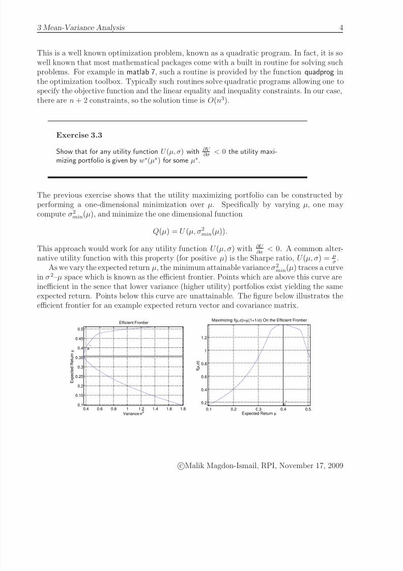
As we vary the expected return µ, the minimum attainable variance σ2min(µ) traces a curvein σ2–µ space which is known as the efficient frontier. Points which are above this curve areinefficient in the sence that lower variance (higher utility) portfolios exist yielding the same

expected return. Points below this curve are unattainable. The figure below illustrates theefficient frontier for an example expected return vector and covariance matrix.

0.4 0.6 0.8 1 1.2 1.4 1.6 1.80.1

0.15

0.2

0.25

0.3

0.35

0.4

0.45

0.5

Efficient Frontier

Variance σ2

E x p e c t e d R e t u r n µ

µ*

0.1 0.2 0.3 0.4 0.5

0.2

0.4

0.6

0.8

1

1.2

Maximizing f(µ,σ)=µ(1+1/ σ) On the Efficient Frontier

Expected Return µ

f ( µ , σ

)

µ*





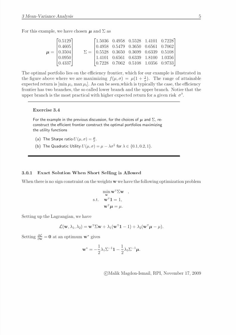
For this example, we have chosen µ and Σ as

µ =

0.51290.46050.3504

0.09500.4337

Σ =

1.5036 0.4958 0.5528 1.4101 0.72280.4958 0.5479 0.3650 0.6561 0.70620.5528 0.3650 0.3699 0.6339 0.5108

1.4101 0.6561 0.6339 1.8100 1.03560.7228 0.7062 0.5108 1.0356 0.9733

The optimal portfolio lies on the efficiency frontier, which for our example is illustrated inthe figure above where we are maximizing f (µ, σ) = µ(1 + 1

σ). The range of attainable

expected return is [min µi, max µi]. As can be seen,which is typically the case, the efficiencyfrontier has two branches, the so called lower branch and the upper branch. Notice that theupper branch is the most practical with higher expected return for a given risk σ2.

Exercise 3.4

For the example in the previous discussion, for the choices of µ and Σ, re-construct the efficient frontier construct the optimal portfolios maximizingthe utility functions

(a) The Sharpe ratio U (µ, σ) = µσ

.

(b) The Quadratic Utility U (µ, σ) = µ − λσ2 for λ ∈ {0.1, 0.2, 1}.

3.0.1 Exact Solution When Short Selling is Allowed

When there is no sign constraint on the weights w we have the following optimization problem

minw

wTΣw ,

s.t. wT1 = 1,

wTµ = µ.

Setting up the Lagrangian, we have

L(w, λ1, λ2) = wTΣw + λ1(wT1 − 1) + λ2(wTµ − µ).

Setting ∂ L∂ w

= 0 at an optimum w∗ gives

w∗ = −1

2λ1Σ−11 −

1

2λ2Σ−1µ.





We are assuming that Σis invertible, which in particular means that there is no risk freeasset (as then a row and column in Σ which is all 0), and no security is a linear combinationof some other set of securities. The constraints require that

1TΣ−11λ1 + 1TΣ−1µλ2 = −2,

µT

Σ−1

1λ1 + µT

Σ−1

µλ2 = −2µ.

In matrix format we have 1TΣ−11 1TΣ−1µ

1TΣ−1µ µTΣ−1µ

λ1λ2

= −2

1µ

.

Define α = 1TΣ−11, β = 1TΣ−1µ and γ = µTΣ−1µ. Taking the inverse of the matrix, onecan solve for λ1, λ2.

Exercise 3.5

Solve for λ1, λ2 above.

(a) Show that the inverse of the 2 × 2 matrix defined by α , β , γ exists.

[Hint: Show that its determinant is αγ − β 2 > 0 using the Cauchy-Schwarz inequality.]

(b) Show that

λ1 = −2(γ − βµ)

αγ − β 2, λ2 = −

2(αµ − β )

αγ − β 2.

(c) Show that the optimal portfolio is given by

w∗ =

γ − βµ

αγ − β 2Σ−1

1 +αµ − β

αγ − β 2Σ−1µ.

(d) Let wg be the portfolio with globally minimum variance satisfying thebudget constraint wT

1 = 1. Show that

wg =1

αΣ−1

1.

(e) Define a second portfolio wµ = 1

β Σ−1µ. Verify that

wT

g1 = 1, wT

µ1 = 1.

(f) Show thatw∗ = ρwg + (1 − ρ)wµ,

where ρ = αγ −αβµαγ −β 2

.





The result of the previous exercise is an example of a separation result which says that theefficient portfolios on the efficient frontier are a linear combination of two portfolios, wg, wµ.The portfolios wg, wµ can be viewed as two “mutual funds” and this result says that in

the mean-variance optimal world, two mutual funds suffice (wg, wµ) – the global minimumvariance portfolio, and a second portfolio wµ. Every optimal portfolio can be expressed as alinear combination of these. In fact, the efficient frontier has a very simple parabolic form.

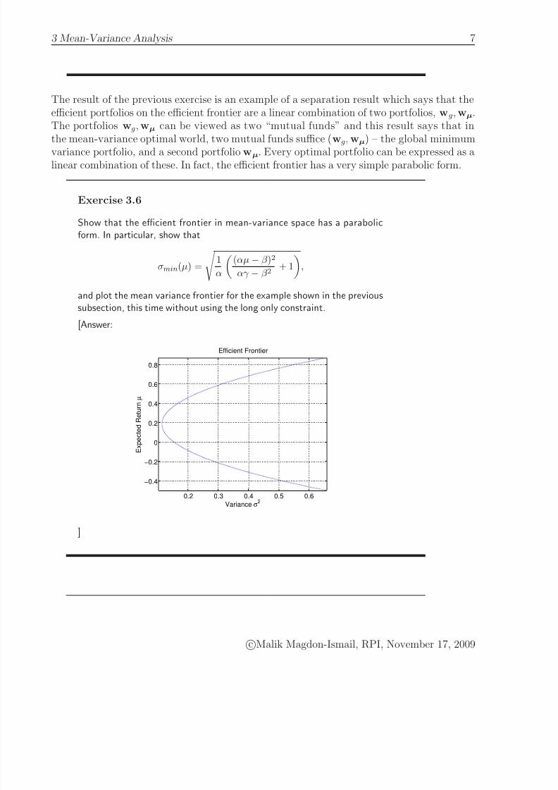
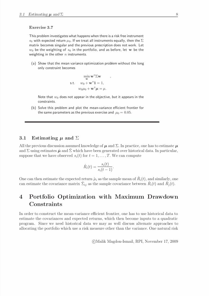
Exercise 3.6

Show that the efficient frontier in mean-variance space has a parabolicform. In particular, show that

σmin(µ) = 1α(αµ − β )2

αγ − β 2

+ 1,

and plot the mean variance frontier for the example shown in the previoussubsection, this time without using the long only constraint.

[Answer:

0.2 0.3 0.4 0.5 0.6

−0.4

−0.2

0

0.2

0.4

0.6

0.8

Efficient Frontier

Variance σ2

E x p e c t e d R e

t u r n µ

]




3.1 Estimating µ and Σ 8

Exercise 3.7

This problem investigates what happens when there is a risk free instruments0 with expected return µ0. If we treat all instruments equally, then the Σmatrix becomes singular and the previous prescription does not work. Letw0 be the weighting of s0 in the portfolio, and as before, let w be theweighting in the other n instruments.

(a) Show that the mean variance optimization problem without the longonly constraint becomes

minw

wTΣw ,

s.t. w0 + wT1 = 1,

w0µ0 + wTµ = µ.

Note that w0 does not appear in the objective, but it appears in theconstraints.

(b) Solve this problem and plot the mean-variance efficient frontier forthe same parameters as the previous exercise and µ0 = 0.05.

3.1 Estimating µ and Σ

All the previous discussion assumed knowledge of µ and Σ. In practice, one has to estimate µ

and Σ using estimates µ̂ and Σ̂ which have been generated over historical data. In particular,

suppose that we have observed si(t) for t = 1, . . . , T . We can compute

R̂i(t) =si(t)

si(t − 1).

One can then estimate the expected return µ̂i as the sample mean of R̂i(t), and similarly, onecan estimate the covariance matrix Σ̂ij as the sample covariance between R̂i(t) and R̂ j(t).

4 Portfolio Optimization with Maximum Drawdown

Constraints

In order to construct the mean-variance efficient frontier, one has to use historical data toestimate the covariances and expected returns, which then become inputs to a quadraticprogram. Since we need historical data we may as well discuss alternate approaches toallocating the portfolio which use a risk measure other than the variance. One natural risk




4 Portfolio Optimization with Maximum Drawdown Constraints 9

measure is the maximum drawdown (MDD). Suppose that an instrument si has values si(t).Let µi(t) be the return up to time t for instrument i,

µi(t) =si(t)

si(0).

Suppose we have a portfolio which invests a fraction wi of the wealth at time 0 in instrumentsi. Then for the portfolio, we have that the return up to time t is given by

Rw(t) =ni=1

wiµi(t),

= wTµ(t),

where µ(t) is the vector containing the returns of the instruments up to time t. We definethe MDD of the portfolio over the time period [0, T ] as the MDD of the return curve R w,where the return curve for the portfolio is given by,

R w =

Rw(1)Rw(2)

...Rw(T )

,

MDD = MDD(R w).

The final return of the portfolio is

R(w) = Rw(T ),

= wT

µ(T ).

As with the mean-variance analysis, we may consider maximizing a utility function

U (R(w),MDD(R w)),

which for fixed R(w) is decreasing in MDD(R w). In this case, we need to construct themean-MDD efficient frontier, which corresponds to constructing the portfolio w∗(µ) whichminimizes the MDD while attaining a specified return µ. Equivalently, we can consider theproblem of constructing the optimal portfolio w∗(MDD) which maximizes the return whileconstrained to having a specified MDD.

Exercise 4.8

Show that the efficient frontier obtained by minimizing the MDD for aspecified return and the efficient frontier obtained by maximizing the returnfor a specified MDD are equivalent (under some mild conditions).





We will obtain the mean-MDD efficient frontier by constructing the optimal portfolio whichmaximizes the return while attaining a specified MDD. For a particular instrument, we defineits return series as

R i =

µi(1)µi(2)

...µi(T )

,

and we define the return matrix as the matrix whose columns are the individual instrumentreturn series,

R =

R 1 R 2 · · · R n

=

µT(1)µT(2)

...µT(T )

.

Notice thatR w = R w.

To obtain the efficient frontier, we need to maximize the return subject to the MDD con-straint. Specifically, we need to solve the optimization problem

maxw

wTµ(T ),

s.t. MDD(R w) ≤ mdd,

wT1 = 1,

w ≥ 0.

Except for the ugly looking MDD constraint, this looks like a linear program. Fortunately,it turns out that the MDD constraint can be rephrased in terms of linear inequalities, andso we will end up with a linear program. Specifically lets introduce the drawdown to time t,DD(t),

DD(t) = maxi≤t

Rw(i) − Rw(t).

DD(t) is the drawdown from the previous high in getting to time t. The reason for introduc-ing the function DD(t) is that the MDD is equal to DD(t∗) for some time t∗. In particular,the time for which the DD(t) is maximized.

Exercise 4.9

Show that M DD = maxt DD(t).





Exercise 4.10

Show that the constraint M DD ≤ mdd is equivalent to the T constraints

DD(1) ≤ mdd ,

DD(2) ≤ mdd ,

... ,

DD(T ) ≤ mdd .

Thus, we may replace the MDD constraint with T constraints on the DD. Let z t be the

maximum of Rw(i) up to t. Then

DD(t) = z t − Rw(t).

The z t can be defined recursively by z 0 = 0, and

z t = max(z t−1, Rw(t)).

Combining the MDD constraint with this recursion, we obtain a set of inequalities whichneed to be satisfied for t = 1, . . . , T ,

z t − Rw(t) ≤ mdd,

z t−1 ≤ z t,Rw(t) ≤ z t.

We introduce the auxiliary variable z, and then in vector form, these inequalities becomez 0 = 0 and

z − R w ≤ mdd · 1,

z t−1 ≤ z t for t = 1, . . . , T ,

R w ≤ z.

These inequalities are implied by the MDD constraint. In particular any set of z 0, z which

satisfy these constraints implies that MDD(R w) ≤ mdd.

Exercise 4.11

Show that for any set of z0, z satisfying the above constraints, DD(t) ≤zt − Rw(t) ≤ mdd and hence M DD(R w) ≤ mdd.




4.1 Integer Portfolio Constraints and Mixed Integer Linear Programming 12

For the z t to actually equal the maxima and for this set of constraints to be equivalent tothe MDD constraint, the z t should be as small as possible. It turns out that by trying tomaximize the return, this is implicitly accomplished. We thus have the following equivalent

optimization problem to compute the efficient frontier,

maxw,z,z0

wTµ(T ),

s.t. z 0 = 0,

z − R w ≤ mdd · 1,

z t−1 ≤ z t for t = 1, . . . , T ,

R w ≤ z,

wT1 = 1,

w ≥ 0.

The variables z 0, z are called auxilliary variables, and it is common to introduce such variablesin transforming a more complex optimization problem into a linear program. We now havea linear program with 3T + 1 additional constraints for a total of n + 3T + 2 constraints.Solving this LP is thus in O((n + 3T )3) using standard packages like linprog in matlab.

Exercise 4.12

While we have argued that the solution to the LP is equivalent to thesolution to the original constrained MDD problem, we have not actuallyshown it.

(a) Show that any solution w, z, z0 to this LP results in an allocation w

which is feasible for the original MDD-constrained optimization.

(b) Show that for any solution w to the original MDD-constrained opti-mization, there is a feasible point having the same w and appropri-ately chosen z, z0 which is feasible for this LP.

(c) Show that the allocation w which results from a solution to this LPis a solution to the MDD-constrained return optimization problem.

4.1 Integer Portfolio Constraints and Mixed Integer Linear Pro-

gramming

One natural way in which an integer constraint appears is when securities can only be boughtin integral amounts. Another which we present through an example is when a particular




4.1 Integer Portfolio Constraints and Mixed Integer Linear Programming 13

investment si may be invested in at some minimum level mi up to some maximum level M iand there is a fixed cost f i to taking on this investment. We assume that all these costsare expressed as fractions of the initial wealth W 0. In such cases, it is typically useful tointroduce the binary variables yi ∈ {0, 1} which indicate whether or not the investment isundertaken. In this case, we have that wi ∈ {0} ∪ [mi,M i], which can be summarized by the

linear constraints

M iyi ≥ wi ≥ miyi.

These constraints automatically imply that if yi = 0, then wi = 0 and if yi = 1 thenwi ∈ [mi,M i]. The budget constraint is

iwi+f iyi ≤ 1. Thus we see that all the constraints

and the objective can be expressed in terms of linear inequalities.The only catch is that someof the variables are binary. The resulting optimization problem is called a mixed program .If the objective and all constraints are linear equality or inequality constraints, it is a mixed integer linear program (MILP). For example, when one is trying to simply maximize thereturn under such constraints, we have

maxw,y

wTµ,

s.t. yi ∈ {0, 1},

wi ≤ M iyi,

miyi ≤ wi,ni=1wi + f iyi ≤ 1,

w ≥ 0.

Such problems are typically very hard to solve exactly (even in the computational sense)

and one has to resort to approximation algorithms. We will not elaborate further, except tosay that there is a vast literature on approximate solution of integer linear programs.


computational finance – portfolio optimization and capital allocation

Documents