computational fluid dynamics analysis on the course

Journal of Mechanical Engineering and Sciences

ISSN (Print): 2289-4659; e-ISSN: 2231-8380

Volume 11, Issue 3, pp. 2919-2929, September 2017

© Universiti Malaysia Pahang, Malaysia

DOI: https://doi.org/10.15282/jmes.11.3.2017.12.0263

2919

Computational fluid dynamics analysis on the course stability of a towed ship

A. Fitriadhy*, M.K. Aswad, N. Adlina Aldin, N. Aqilah Mansor, A.A. Bakar, and

W.B. Wan Nik

1Program of Maritime Technology, School of Ocean Engineering,

Universiti Malaysia Terengganu, Malaysia.

*Email: [email protected]

Phone: +6096683856; Fax: +6096683193

ABSTRACT

Due to the highly complex phenomenon of a ship towing system associated with the

presence of a dynamic nonlinear towline tension, a reliable investigation allowing for an

accurate prediction of the towed ship’s course stability is obviously required. To achieve

the objective, a Computational Fluid Dynamic simulation approach is proposed by

investigating attainable and precise course stability outcomes, whilst a hydrodynamic

description underlying the rationale behind the results is explained. Several towing

parameters such as various towline lengths and tow point locations with respect to the

centre of gravity of the barge have been taken into account. Here, tug and barge is

employed in the simulation as the tow and towed ship, respectively. In addition, a towing

velocity is constantly applied on the tug. The results revealed that the course stability of

the towed ship increases in the form of more vigorous fishtailing motions as the towline

length subsequently increases from 1.0 to 3.0. Meanwhile, the increase of tow point

location from 0.5 to 1.0 leads to a significant improvement in the course stability of the

towed ship, as indicated by the reduction of the sway and yaw motions by 227% and 328%,

respectively. It is concluded that the increase of tow point location is a recommended

decision to achieve a better towing course stability for the barge.

Keywords: CFD; course stability; towline length; tow point; towline tension.

INTRODUCTION

Recognising the inherent advantages offered by the typical ship towing system, it has

become frequently used in inland waterway/ocean transportation, military operations and

in the salvage of disabled ships [1]. In this transportation mode, an improper towing

system may introduce severe towing instability and directly lead to accidents such as

collisions with other vessel or onshore structures which may probably occur, especially

in confined waters with high sea traffic. Additionally, this type of accident may often lead

to loss of property, human lives and environmental issues [2]. An extensive investigation

regarding the course stability of the towed ship is therefore required. Several researchers

have presented many theoretical approaches to analyse the course stability of the ship’s

towing system. [3] proposed a numerical theory of barge dynamic stability in towing

operations with and without the presence of skegs. Then, [4], [5]and [6] developed

numerical simulations where the effects of the towline length and tow point locations to

the course stability of a towed ship have been addressed. [7], [8] and [9] performed

numerical analyses of towed ships’ stability in steady winds. Furthermore, experimental

https://doi.org/10.15282/jmes.11.3.2017.12.0263

mailto:[email protected]


2920

model tests have been conducted at Towing-Tank to investigate the course stability of a

tanker as the towed ship in [10] and [11]. In particular, this approach is relatively

expensive, time-consuming and even impractical for various tests on the ship's towing

system. To accommodate such demands, a proper simulation approach aimed at gaining

reliable predictions on the course stability of the ship towing system as compared to

analytical/numerical approaches is needed.

This paper presents a CFD simulation used to predict the course stability of a

towed ship in calm waters. Here, the commercial CFD called FLOW3D version 10.1 is

utilised by applying the incompressible unsteady Reynolds-Averaged Navier Stokes

equations (RANS) in simulation, in which both the RANS equation and continuity

equations are discretised using the finite volume method based on Volume of Fluid (VOF)

to deal with the nonlinear free surface. In addition, the computational domain with

adequate numbers of grid meshes specifically for the towed ship model has been carefully

determined before the simulations. Basically, this is solved by the means of a mesh

independent study conducted to select the optimal domain discretisation. Several

parameters such as various towline lengths ratios (ℓ′=ℓ/𝐿) from 1.0 up to 3.0 and tow

point locations (ℓ′𝑏=ℓ𝑏/𝐿) from 0.5 up to 1.0 are taken into consideration. The results are

comprehensively discussed to point out the effect of towline lengths and tow point

locations with their dependencies on the course stability of the towed ship, which is

presented in the form of sway and yaw motions. Correspondingly, the towline tension is

also captured and properly explained with regard to the aforementioned parametric

studies.

METHODS AND MATERIALS

Governing Equations

The CFD flow solver in FLOW-3D version 10.1 is based on the incompressible unsteady

RANS equations in which the solver applies the Volume of Fluid (VOF) to track the free

surface elevation. The interface between fluid and solid boundaries is simulated using

the fractional area volume obstacle representation favour method. This method computes

the open area and volume in each cell to define the area that is occupied by the obstacle.

Continuity and Momentum Equations

The continuity and momentum equations for a moving object and the relative transport

equation for VOF function are [12]:

1.

f f

f

VVuA

t t

(1)

1 1

. .( )f f

f

uuA u A G

t V

(2)

1

.f

f

f f

VF FFuA

t V V t

(3)

where 𝜌 is the density of the fluid, �⃗� is the fluid velocity, 𝑉𝑓 is the volume fraction, 𝐴𝑓 is

the area fraction, 𝑝 is the pressure, 𝜏 is the viscous stress tensor, 𝐺 denotes gravity, and

𝐹 is the fluid fraction.

In the case of the coupled General Moving Object’s (GMO) motion, Eqs. (1) and

(2) are solved at each time step, the location of all moving objects recorded, and the area

Fitriadhy et al. / Journal of Mechanical Engineering and Sciences 11(3) 2017 2919-2929

2921

and volume fractions updated using the FAVOR technique. Equation (3) are solved with

the source term −𝜕𝑉𝑓

𝜕𝑡 on the right-hand side, which is computed as

. /f

obj obj cell

VU nS V

t

(4)

where 𝑆𝑜𝑏𝑗 is the surface area, �⃗� surface normal vector,�⃗⃗� obj is the velocity of the moving

object at a mesh cell, and 𝑉𝑐𝑒𝑙𝑙 is the total volume of the cell [12].

Turbulence Model

The transport equation for 𝑘𝑇 includes the convection and diffusion of the turbulent kinetic

energy, the production of turbulent kinetic energy due to shearing and buoyancy effects,

diffusion, and dissipation due to viscous losses within the turbulent eddies. Buoyancy

production only occurs if there is a non-uniform density in the flow, and includes the

effects of gravity and non-inertial accelerations. The transport equation is:

1

T

T T T Tx y z T T T

F

k k k kuA vA wA P G Diff

kt V x y z

(5)

where 𝑉𝐹, 𝐴𝑥,, 𝐴𝑦 and 𝐴𝑧 are FLOW-3D’s FAVOR™ functions, and 𝑃𝑇 is the turbulent

kinetic energy production:

2 2 22 ( ) 2 ( ) 2 ( )

( ) ( ) ( ) ( )( ( )

( )( )

x y z

T x y z x

F

z y

u v u wA A R A

x y x z

v u v v u v u w u wP CSPRO R A A R A A R

pV x y x x y x z x z x

v w v wR A A R

z y z y

(6)

where CSPRO is a turbulence parameter.

In the case of turbulent conditions, the 𝑘 − 𝜀 model is proposed where 𝑘𝑇 and 𝜀𝑇 are

the turbulent kinetic energy and turbulent dissipation energy, respectively. Two transport

equations for the turbulent kinetic energy 𝑘𝑇 and its dissipation 𝜀𝑇 which is so-called the

𝑘 − 𝜀 model is used in the computational simulation. It is reasonable since this equation

model provides more reliable approximations to many types of flows [12] .In addition,

the 𝑘 − 𝜀 model is quite economical in terms of CPU time, compared to for example the

SST turbulence model, which increases the required CPU time by nearly 25%. [12] [13,

14] stated that the 𝑘 − 𝜀 model reduces computational time and resources by reducing the

number of nodes in the near wall regions, thus allowing for more probing simulation and

trial geometries.

Body Motion Computation

The body motion is analysed in a space-fixed Cartesian coordinate system which is a part

of the global coordinate system. The governing equation of the six degree of freedom

(DOF) of a rigid body motion can be expressed in this coordinate system as

( )C

dmv f

dt

(7)

( . )C C C

dM m

dt

(8)


2922

Index C denotes the centre of mass of the body, m denotes the mass of the body, 𝑣 𝑐

the velocity vector, 𝑀𝑐is the tensor of the moments of inertia, �⃗⃗� c is the angular velocity

vector,𝑓 denotes the resulting force vector, and �⃗⃗� c denotes the resultant moment vector

acting on the body [15] [16]. The resultant force 𝑓 has three components; surface force,

field forces and external forces:

( ). bS V

f T I ndS bdV fE (9)

Here, 𝜌𝑏 is the density of the body. The only field force considered is gravity, so the

volume integral of above equation (right hand side) is reduced to 𝑚𝑔 , where 𝑔 is the

gravity acceleration vector. The vector 𝑓�⃗� denotes the external forces acting in the

body [2].

Simulation Conditions

Principal Data of Ship

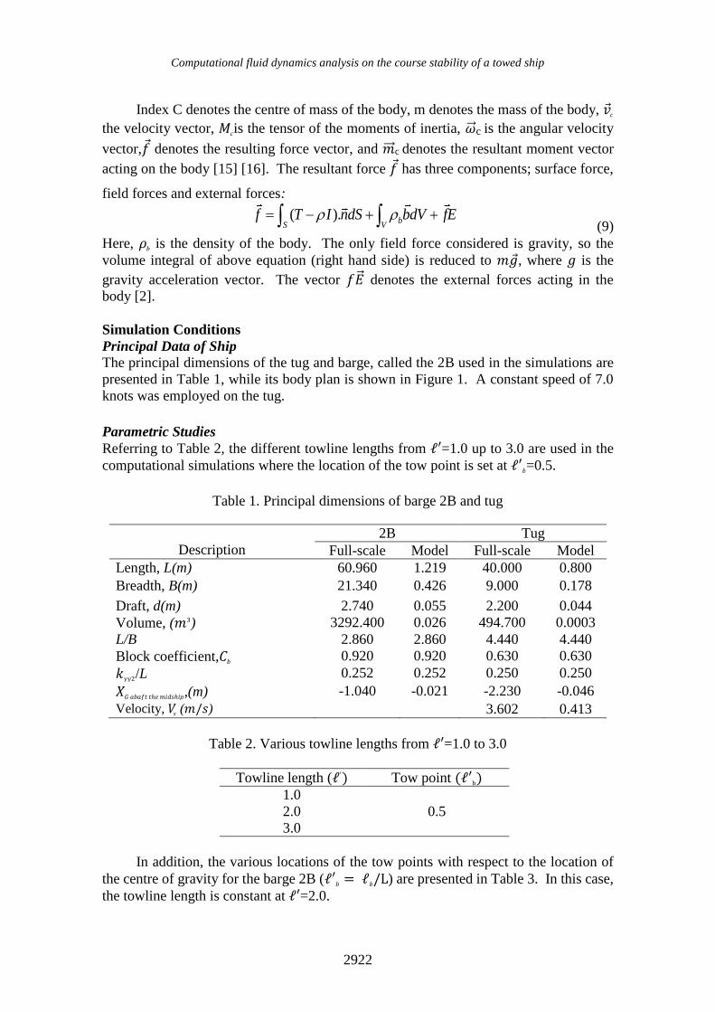
The principal dimensions of the tug and barge, called the 2B used in the simulations are

presented in Table 1, while its body plan is shown in Figure 1. A constant speed of 7.0

knots was employed on the tug.

Parametric Studies

Referring to Table 2, the different towline lengths from ℓ′=1.0 up to 3.0 are used in the

computational simulations where the location of the tow point is set at ℓ′𝑏=0.5.

Table 1. Principal dimensions of barge 2B and tug

Description

2B Tug

Full-scale Model Full-scale Model

Length, L(m) 60.960 1.219 40.000 0.800

Breadth, B(m) 21.340 0.426 9.000 0.178

Draft, d(m) 2.740 0.055 2.200 0.044

Volume, (𝑚3) 3292.400 0.026 494.700 0.0003

L/B 2.860 2.860 4.440 4.440

Block coefficient,𝐶𝑏 0.920 0.920 0.630 0.630

𝑘𝑦𝑦2/L 0.252 0.252 0.250 0.250

𝑋𝐺 𝑎𝑏𝑎𝑓𝑡 𝑡ℎ𝑒 𝑚𝑖𝑑𝑠ℎ𝑖𝑝,(m) -1.040 -0.021 -2.230 -0.046

Velocity, 𝑉𝑠 (𝑚/𝑠) 3.602 0.413

Table 2. Various towline lengths from ℓ′=1.0 to 3.0

Towline length (ℓ′) Tow point (ℓ′b)

1.0

2.0 0.5

3.0

In addition, the various locations of the tow points with respect to the location of

the centre of gravity for the barge 2B (ℓ′𝑏 = ℓ𝑏/L) are presented in Table 3. In this case,

the towline length is constant at ℓ′=2.0.


2923

Figure 1. Body plan of tug (left) and barge (right).

Table 3: Various tow points from ℓ′𝑏= 0.5 up to 1.0

Computational Domain and Boundary Conditions

The computational domain uses a structured mesh that is defined in a Cartesian. Referring

to Figure 2, the boundary condition was marked in the mesh block. The boundary

condition at the X-max boundary is specified velocity so that there is flow of water. In

order to save computational time, a velocity of 0.413 m/s is given to the water at the X-

max boundary. For X-min, Y-max and Y-min outflow are used to prevent reflection,

while Z-min and Z-max use symmetry. The boundary conditions for this simulation are

as shown in Table 4.

Figure 2. Boundary conditions.

Figure 3. Meshing generation.

The tug and barge are coupled together using a towline. The barge is inclined by

15o with respect to the initial z-axis. The tug which acts as the tow ship was assigned as

the prescribed motion, while the barge as the towed ship was set as the coupled motion in

the X-translational, Y-translational and Z-rotational motions (surge, sway and yaw

motions). The towline is set as a massless elastic rope with a spring coefficient of 2.0

N/m. Based on the FLOW3D v10.1.1, the average duration of every simulation was about

70-80 hours (4 parallel computations) on a HP Z820 workstation PC with processor Intel

(R) Xeon (R) CPU ES-2690 v2 @ 3.00 GHz (2 processors) associated with an installed

memory [16] of 32.0 GB and a 64-bit Operating System.

Towline length(ℓ′ ) Tow point (ℓ′𝑏) 0.5

2.0 0.75

1.0

Specified

Velocity Mesh

block 1

Mesh

block 2 Symmetry

Outflow

Outflow

Outflow

Symmetry


2924

Table 4. Boundary conditions.

Boundary Condition

Mesh block 1 Mesh block 2

Xmin Outflow Symmetry

Xmax Specified Velocity Symmetry

Ymin Outflow Symmetry

Ymax Outflow Symmetry

Zmin Symmetry Symmetry

Zmax Symmetry Symmetry

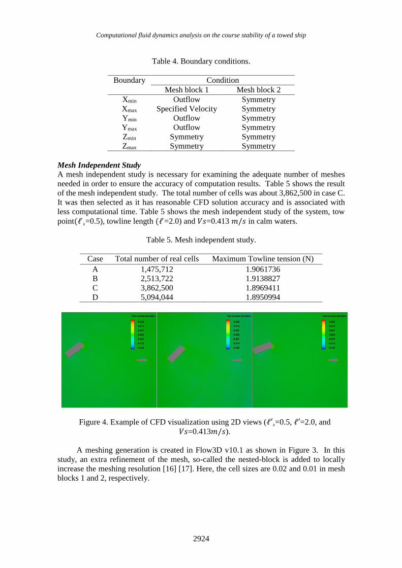
Mesh Independent Study

A mesh independent study is necessary for examining the adequate number of meshes

needed in order to ensure the accuracy of computation results. Table 5 shows the result

of the mesh independent study. The total number of cells was about 3,862,500 in case C.

It was then selected as it has reasonable CFD solution accuracy and is associated with

less computational time. Table 5 shows the mesh independent study of the system, tow

point(ℓ′𝑏=0.5), towline length (ℓ′=2.0) and 𝑉𝑠=0.413 𝑚/𝑠 in calm waters.

Table 5. Mesh independent study.

Case Total number of real cells Maximum Towline tension (N)

A 1,475,712 1.9061736

B 2,513,722 1.9138827

C 3,862,500 1.8969411

D 5,094,044 1.8950994

Figure 4. Example of CFD visualization using 2D views (ℓ′𝑏=0.5, ℓ′=2.0, and

𝑉𝑠=0.413𝑚/𝑠).

A meshing generation is created in Flow3D v10.1 as shown in Figure 3. In this

study, an extra refinement of the mesh, so-called the nested-block is added to locally

increase the meshing resolution [16] [17]. Here, the cell sizes are 0.02 and 0.01 in mesh

blocks 1 and 2, respectively.


2925

RESULTS AND DISCUSSION

Figures 5-8 show that the CFD simulations have been successfully carried out to predict

the course stability of the towing system at various towline lengths and tow point

locations. The simulation’s sway and yaw motions associated with the towline tension

are discussed accordingly.

Effect of Towline Length

Figure 5 shows the characteristics of the sway and yaw motions and the dynamic towline

tension at various towline lengths from ℓ′=1.0 to 3.0. Extending the towline length ℓ′ from 1.0 to 2.0 and 3.0 had resulted in an increase of sway motion of the towed ship by

41.6%. This unstable towing mainly occurred due to the unwieldy amplitude of her

heading angle and yaw rate associated with the spacious amplitude of her fishtailing

motion. On the other hand, the slewing/fishtailing period of 2B was lower by 10% as ℓ′ was increased from 1.0 to 3.0. Similar to what was reported by Fitriadhy et al. [6], the

increment of towline length had relatively smaller influence on the entire amplitude

motion performance of the barge. Although the increase of towline lengths was

insignificant in reducing the sway motions, the course stability of the 2B had improved

as commented on in Fitriadhy and Yasukawa [4]. Correspondingly, the maximum tension

force had decreased by 7.8% as ℓ′ was increased from 1.0 to 3.0. Regardless of the

maximum value of the free surface elevation, the reason can be explained by the fact that

the 2B experienced more vigorous sway motions when the shorter towline length was

employed (see Figure 6).

Figure 5. Characteristics of 2B’s sway and yaw motions associated with towline

tension at various towline lengths


2926

Figure 6. Free surface elevation, ℓ′𝑏= 0.5, ℓ′= 1.0 (a), ℓ′= 2.0 (b), ℓ′= 3.0 (c),

𝑉𝑠=0.413𝑚/𝑠.

Effect of Tow Point Location

The characteristics of the sway and yaw motions associated with the dynamic towline

tension at various tow point locations are displayed in Figure 7. Similar to what was

remarked in the numerical simulation by Fitriadhy et al. [5], the subsequent increase of

tow points ℓ′𝑏 from 0.5 to 0.75 and 1.0 had resulted in the significant reduction of the

sway and yaw motions. It is noted here that the yaw motion decreased by 87.67% and

128% as ℓ′𝑏 is increased from 0.5 to 0.75 and 0.75 to 1.0, respectively. Inherently, the

course stability of 2B had notably improved. Meanwhile, the existence of this favourable

effect had sufficiently led to an attenuation of the dynamic towline tension. Evidently,

the increase in the tow point is an effective way of recovering the towing instability and

indeed, may prevent the towline’s breakage [18]. Referring to Figure 8, the presence of

higher waves at the bow region of 2B with ℓ′𝑏=1.0 was proportional with the higher

resistance (high pressure) which inherently reduced her sway and yaw motions. These

will decrease the unwieldy slewing motion and lead to better course stability, as noted

by Fitriadhy and Yasukawa [4].

a) ℓ′𝑏= 0.5, ℓ′=1.0

b) ℓ′𝑏= 0.5, ℓ′=2.0

c) ℓ′𝑏= 0.5, ℓ′=3.0


2927

Figure 7. Characteristics of sway and yaw motions of 2B associated with towline

tension at various tow points.

Figure 8. Free surface elevation,, ℓ′𝑏=0.5 (a), ℓ′𝑏=0.75 (b), ℓ′𝑏=1.0 (c)

ℓ′=2.0,𝑉𝑠=0.413 𝑚/𝑠

a) ℓ′𝑏= 0.5, ℓ′=2.0

b) ℓ′𝑏= 0.75, ℓ′=2.0

c) ℓ′𝑏= 1.0, ℓ′=2.0


2928

CONCLUSIONS

The computational fluid dynamics analysis on the course stability of a ship’s towing

system was successfully performed using the Flow3D version 10.1 software. The effects

of different towline lengths and tow point locations have been appropriately investigated.

The simulation results are drawn as follows:

The increase of towline length (ℓ′) from 1.0 up to 3.0 was significant in improving

the course stability of the barge as indicated by the decrease in the reduction of

sway and yaw motions. However, the towline tension also decreased by 7.8%,

which may prevent impulses in the towline that threaten the towing safety.

The course stability of the towed ship is significantly improved due to the

substantial reduction of the sway and yaw motions by 227% and 328% as the tow

point (ℓ′𝑏) was increased from 0.5 to 0.75 and from 0.75 to 1.0, respectively.

Concurrently, this resulted in the sufficient reduction of towline tension by 71.6%

as the tow point was changed from ℓ′𝑏=0.5 to 1.0.

In general, the increase in tow point had resulted in better course stability of towing

compared to increases in towline ones. Correspondingly, these CFD results are useful as

preliminary prediction for the course stability of the towing, which deals with navigation

safety during towing operations.

ACKNOWLEDGMENT

The authors would like to thank Ministry of Higher Education (MOHE)-Malaysia for

the financial Research Grant VOT. 59414.

REFERENCES

[1] Fitriadhy A, Yasukawa H, Maimun A. Theoretical and Experimental Analysis of a Slack

Towline Motion on Tug-towed Ship during Turning. Ocean Engineering. 2015;99:95-

106.

[2] Yan S, Huang G. Dynamic Performance of Towing System-Simulation and Model

Experiment. OCEAN1996.

[3] Lee M-L. Dynamic Stability of Nonlinear Barge-towing System. Applied Mathematical

Modelling. 1989;13:693-701.

[4] Fitriadhy A, Yasukawa H. Course Stability of a Ship Towing System. Ship Technology

Research. 2011;58:4-23.

[5] Fitriadhy A, Yasukawa H, Yonedac T, Kohd K, Maimund A. Analysis of an

Asymmetrical Bridle Towline Model to Stabilise Towing Performance of a Towed Ship.

Jurnal Teknologi (Sciences & Engineering). 2014;66:151-6.

[6] Fitriadhy A, Yasukawa H, Nik WBW, Bakar AA. Numerical Simulation of Predicting

Dynamic Towline Tension on a Towed Marine Vehicle. In: International Conference on

Ships and Offshore Structures ICSOS 2016. Hamburg, Germany; 2016.

[7] Yasukawa H, Hirono T, Nakayama Y, Koh K. Course Stability and Yaw Motion of a

Ship in Steady Wind. Journal of Marine Science and Technology. 2012;17:291-304.

[8] Fitriadhy A, Yasukawa H, Koh K. Course Stability of a Ship Towing System in Wind.

Ocean Engineering. 2013;64:135-45.

[9] Sinibaldi M, Bulian G. Towing Simulation in Wind Through a Nonlinear 4-DOF Model:

Bifurcation Analysis and Occurrence of Fishtailing. Ocean Engineering. 2014;88:366-92.

[10] Varyani K, Barltrop N, Clelland D, Day A, Pham X, Van Essen K, et al. Experimental

Investigation of the Dynamics of a Tug Towing a Disabled Tanker in Emergency Salvage


2929

Operation. International Conference on Towing and Salvage Disabled Tankers2007. p.

117-25.

[11] Kume K, Hasegawa J, Tsukada Y, Fujisawa J, Fukasawa R, Hinatsu M. Measurements

of Hydrodynamic Forces, Surface Pressure, and Wake for Obliquely Towed Tanker

Model and Uncertainty Analysis for CFD Validation. Journal of Marine Science and

Technology. 2006;11:65-75.

[12] FLOW-3D 10.1.1 User Manual: Flow Science Inc.; 2013.

[13] Talaat WM, Hafez K, Banawan A. A CFD Presentation and Visualization For a New

Model that Uses Interceptors to Harness Hydro-energy at the Wash of Fast Boats. Ocean

Engineering. 2017;130:542-56.

[14] Franke Rt, Rodi W. Calculation of Vortex Shedding Past a Square Cylinder with Various

Turbulence Models. Turbulent Shear Flows 8: Springer; 1993. p. 189-204.

[15] Wu C-S, Zhou D-C, Gao L, Miao Q-M. CFD Computation of Ship Motions and Added

Resistance for a High Speed Trimaran in Regular Head Waves. International Journal of

Naval Architecture and Ocean Engineering. 2011;3:105-10.

[16] Saad I, Bari S. CFD Investigation of In-cylinder Air Flow to Optimize Number of Guide

Vanes to Improve ci Engine Performance using Higher Viscous Fuel. International

Journal of Automotive and Mechanical Engineering. 2013;8:1096.

[17] Lam S, Shuaib N, Hasini H, Shuaib N. Computational Fluid Dynamics Investigation on

the Use of Heat Shields for Thermal Management in a Car Underhood. 2012:785.

[18] Zan U, Yasukawa H, Koh K, Fitriadhy A. Model Experimental Study of a Towed Ship's

Motion.

NOMENCLATURE

ℓ′𝑏=ℓ𝑏/𝐿 Ratio of tow point distance to length of barge with respect

to her center of gravity

ℓ′=ℓ/𝐿 Ratio of towline length with respect to length of barge

2B Barge

CFD Computational Fluid Dynamics

RANS Reynolds-Averaged Navier-Stokes equation

VOF Volume of Fluid method

GMO General moving object

FAVOR Fractional Area-Volume Obstacle Representation

computational fluid dynamics analysis on the course

Documents