computational fluid dynamics study of nasal...
TRANSCRIPT
COMPUTATIONAL FLUID DYNAMICS STUDY OF
NASAL CAVITY MODEL
VIZY NAZIRA BINTI RIAZUDDIN
UNIVERSITI SAINS MALAYSIA
2011

COMPUTATIONAL FLUID DYNAMICS STUDY OF NASAL CAVITY MODEL
by
VIZY NAZIRA BINTI RIAZUDDIN
Thesis submitted in fulfillment of the requirements
for the degree of
Master of Science
UNIVERSITI SAINS MALAYSIA
July 2011

ii
ACKNOWLEDGEMENT
Alhamdulillah. Thanks and glory be to Allah (SWT) alone, for giving me this
opportunity, strength and patience to complete my dissertation finally, after all the
challenges and difficulties.
First and foremost, I would like to express my deepest appreciation to my
supervisor; Dr. Kamarul Arifin bin Ahmad, whose encouragement, guidance and support
from the very beginning which enabled me to develop the understanding of the subject.
My sincere thanks to Prof. Dr. Zulkifly Abdullah, Prof. Dr. Ibrahim Lutfi Shuaib,
Dr. Rushdan Ismail, Assoc. Prof. Dr. Suzina Sheikh Abdul Hamid, and Mr. Mohamad
Zihad Mahmud for their continuous thoughtful advice in bringing this research works to
fruition. I would like to acknowledge my research colleague, Mr. Mohammed Zubair for
his invaluable assistance and support throughout the entire research. I would like to
thank all my colleagues for the joyful memories throughout the research.
Special thanks to Mohd Shahadan Mohd Suan, Khairunisa Zulkurnain and my
parents, Riazuddin Ahmad Ali and Norizan Osman for their support and encouragement
that enabled me to endure the hardship of my academic career.
iii
TABLE OF CONTENTS
ACKNOWLEDGEMENT ii
TABLE OF CONTENTS iii
LIST OF TABLES vii
LIST OF FIGURES viii
LIST OF ABBREVIATIONS xii
LIST OF SYMBOLS xiv
ABSTRAK xvi
ABSTRACT
xviii
CHAPTER 1 – INTRODUCTION
1.1 Research Background 1
1.2 Aims and Objectives 3
1.3 Scope of Work 4
1.4 Organization of The Thesis
4
CHAPTER 2 – LITERATURE RIVIEW
2.1 Overview 5
2.2 Anatomy and Physiology of The Human Nasal Cavity 5
2.2.1 Nasal Anatomy 5
2.2.2 Nasal Physiology 8
2.3 Objective measurement methods 9

iv
2.3.1 Rhinomanometry 9
2.3.2 Acoustic Rhinomanometry 10
2.4 Numerical Study of Flow Through The Nasal Cavity 11
2.5 Gender Comparison 19
2.6 Gravity Effect 20
2.7 Plug Flow and Pull Flow Boundary Condition 21
2.8 Summary
22
CHAPTER 3 – MODELLING THE HUMAN NASAL CAVITY
3.1 Overview 23
3.2 3D Computational Model of the Nasal Cavity 24
3.2.1 Procuring CT Scan Data of Human Nasal Cavity 24
3.2.2 Convert 2D CT Scan Images to 3D CAD Data Using Mimics 25
3.2.3 Geometry Creation Using CATIA 28
3.3 Mesh Generation Using GAMBIT 31
3.4 Numerical analysis 33
3.4.1 Governing Equation 33
3.4.2 Turbulence Models 34
3.4.3 Numerical Solver Procedure 35
3.4.4 Boundary Condition Definition
37
v
CHAPTER 4 – RESULTS AND DISCUSSION
4.1 Overview 39
4.2 Grid Dependency Analysis 39
4.3 Geometry Comparison 41
4.4 Model Comparison 44
4.5 Basic Flow Studies 46
4.5.1 Reynolds Number Calculation 46
4.5.2 Velocity 47
4.5.3 Pressure 50
4.5.4 Wall Shear Stress 51
4.5.5 Inspiration Vs Expiration 54
4.5.5.1 Velocity and Pressure Comparison 54
4.5.5.2 Resistance 56
4.5.5.3 Wall Shear Stress 57
4.6 Various Breathing Rates for Inspiration and Expiration 59
4.6.1 Average Velocity 59
4.6.2 Wall Shear Stress 62
4.7 Preliminary Work On Gender Comparison 65
4.7.1 Geometry Comparison 65
4.8 Gravity Effect On Nasal Airflow Due to the Change Of Posture 72
4.9 Effect of Different Boundary Condition On Flow Parameters 76
4.9.1 Nasal Resistance Comparison for Plug-Flow and Pull-Flow 77
4.9.2 Velocity 79

vi
4.9.3 Pressure 81
4.9.4 Wall Shear Stress
82
CHAPTER 5 – CONCLUSION
5.1 Introduction 84
5.2 Major Conclusions Drawn From This Study 84
5.2.1 Basic Airflow Studies 85
5.2.2 Various Breathing Rates for Inspiration and Expiration 86
5.2.3 Gravity Effect On Nasal Airflow Due to the Change Of Posture
86
5.2.4 Effect of Different Boundary Condition On Flow Parameters 87
5.3 Future Works 88
REFERENCES 90
LIST OF PUBLICATIONS 95

vii
LIST OF TABLES
Page
Table 3.1
Boundary condition for pull flow and plug flow 37
Table 4.1
The total length of the nasal cavity based on the gender comparison
66
Table 4.2
Characteristic description of nasal cavity for male and female nasal cavity models
69

viii
LIST OF FIGURES
Page
Figure 2.1
Diagram of the Nasal Cavity- reproduced from the Gray's anatomy of the human body, reproduced from Henry Gray, (1918)
6
Figure 2.2
Coronal section of the main nose airway- reproduced from Zamankhan et al.,(2006)
7
Figure 2.3
Simplified structure of the nasal cavity- reproduced from Tsui Wing Shum, (2009)
7
Figure 2.4
Nose-like model- reproduced from Elad et al., (1993) 12
Figure 2.5
Medial slide of the tree-dimensional finite element mesh of the right nasal cavity- reproduced from Keyhani et al., (1995)
13
Figure 2.6
Computational meshes for subjects A, 12, 14 and 18. Nostrils are shown in blue on the right side of the models and the nasopharynx is on the left- reproduced from Segal et al., (2008)
14
Figure 2.7
Nasal cavity model constructed by Wen et al., (2008) 15
Figure 3.1
Coronal CT scan images along the axial distance of the human nasal cavity
25
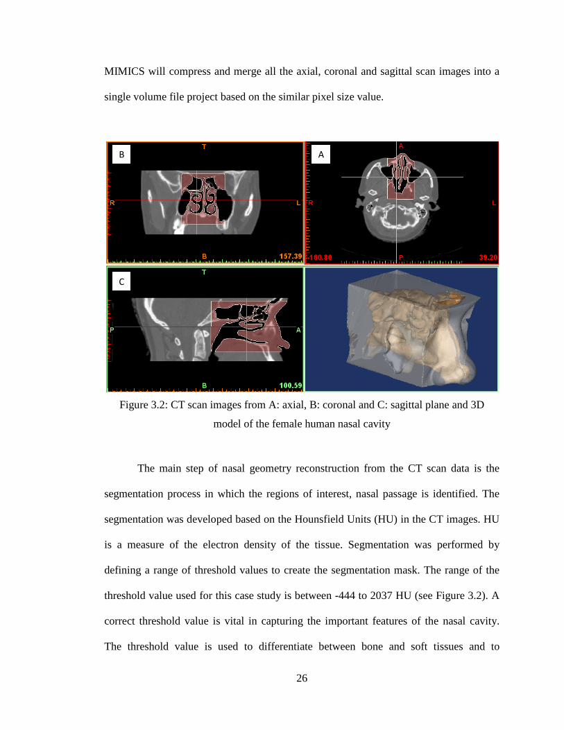
Figure 3.2
CT scan images from A: axial, B: coronal and C: sagittal plane and 3D model of the female human nasal cavity
26
Figure 3.3
Polyline data of the 3D human nasal cavity 28
Figure 3.4
Steps involved in developing 3D model of the nasal cavity using CATIA
30
Figure 3.5
3D computational model of the nasal cavity with surface geometry
31
Figure 3.6
Volume mesh of the 3D computational model of human nasal cavity
32
Figure 3.7 Pressure-based solution method (Fluent User manual) 36

ix
Figure 4.1
Grid independence plot 40
Figure 4.2
Ten cross section area along the axial distance of the nasal cavity
41
Figure 4.3
Ten cross section area through the nasal cavity 42
Figure 4.4
The comparison of cross-sectional area vs. axial distance from anterior to the posterior of the nasal cavity
43
Figure 4.5
Pressure drop vs. inspiratory flow rates compared with previous data
45
Figure 4.6
Average velocity contour along the nasal cavity 48
Figure 4.7
Variation of average velocity along the length of the nasal cavity
49
Figure 4.8
Flow recirculation at the olfactory region 49
Figure 4.9
Comparison between left and right nasal cavity 50
Figure 4.10
Average static pressure along the nasal cavity during inspiration
51
Figure 4.11
Maximum wall shear stress along the axial distance of the nasal cavity (full model)
52
Figure 4.12
Average wall shear stress contour 53
Figure 4.13
Maximum wall shear stress across left and right nasal cavity 54
Figure 4.14
Velocity profile comparison during inspiration and expiration
55
Figure 4.15
Average static pressure along the axial length of the nasal cavity
56
Figure 4.16
Pressure drop value during inspiration and expiration for various flow rates
57
Figure 4.17
Maximum wall shear stress along the axial distance of the nasal cavity
58
Figure 4.18 Average velocity at different flow rates from 7.5 to 40 60
x
L/min during inspiration
Figure 4.19
Model of the nasal cavity showing the olfactory plane 61
Figure 4.20
Average velocity at different flow rates from 7.5 to 40 L/min during expiration
62
Figure 4.21
Maximum wall shear stress values through the axial distance of the nasal cavity during inspiration
63
Figure 4.22
Maximum wall shear stress values through the axial distance of the nasal cavity during expiration
64
Figure 4.23
The comparison of cross section area through the nasal cavity of the human male and female subjects
66
Figure 4.24
The pressure drop value across the nasal cavity 68
Figure 4.25
Variation of Average static pressure with posture 73
Figure 4.26
Effect of change of posture on velocity at 15L/min 73
Figure 4.27
Variation in Max. Wall shear stresses with change of posture
74
Figure 4.28
A: Sitting B: Supine, shows flow variations along a horizontal plane at middle meatus region
75
Figure 4.29 Plug flow boundary condition for inspiration A and expiration B
76
Figure 4.30 Pull flow boundary condition for inspiration A and expiration B
76
Figure 4.31
Nasal Resistance for different airflow rate 77
Figure 4.32
Inspiratory nasal resistance for 15L/min at vestibule, nasal valve, middle section and nasopharynx
78
Figure 4.33
Velocity plot along the axial distance (at 15 L/min) 79
Figure 4.34
Velocity profile for pull flow boundary condition A and plug flow boundary condition B
80
Figure 4.35
Pressure plot for plug and pull flow boundary condition during inspiration A and expiration B
82

xi
Figure 4.36
Maximum wall shear stress values during inspiration 83

xii
LIST OF ABBREVIATIONS
3D Three Dimensional
AMDI Advanced Medical and Dental Institute
AR Atrophic Rhinitis
AAR Active Anterior Rhinometry
CAD Computational Aid Design
CAT Computerized Axial Tomography
CFD Computational Fluid Dynamics
CPU Central Processing Unit
CT Computed Tomography
DSE Digitized Shape Editor
EIM Eddy Interaction Model
ENT Ear, Nose and Throat
HU Hounsfield Units
IBM International Business Machines
IGES Initial Graphics Exchange Specification
LES Large Eddy Simulation

xiii
MRI Magnetic Resonance Imaging
NAR Nasal Airway Resistance
OSA Obstructive Sleep Apnea
RAM Random-Access Memory
RANS Reynolds Average Navier Stoke
SST Shear Stress Transport Model
STP STEP File/Standard for the Exchange of Product File

xiv
LIST OF SYMBOLS
ROMAN SYMBOLS
d Diameter of the nasal inlet
k Turbulent kinetic energy
Re Reynolds number
R Resistance
𝑆𝑆Ф The source term of Ф
t Time
u Velocity vector
V Velocity of the flow
𝑦𝑦 The distance to the wall
𝑢𝑢𝜏𝜏 Friction velocity
𝑣𝑣 Kinematic viscosity of the fluid flow
GREEK SYMBOLS
Г Diffusion coefficient
𝜕𝜕 Partial differential equation
Ф General scalar
𝜀𝜀 Dissipated rate of k
ω Specific rate of dissipation of k
𝜌𝜌 Fluid density
𝜇𝜇 Dynamic viscosity of the air

xv
ΔP Pressure drop
SUBSCRIPTS
vel Velocity
SUPERSCRIPT
+ Variable expressed in wall units

xvi
KAJIAN PENGKOMPUTERAN DINAMIK BENDALIR TERHADAP MODEL
RONGGA HIDUNG
ABSTRAK
Pemahaman terhadap sifat-sifat aliran udara di dalam rongga hidung adalah sangat
penting dalam menentukan fisiologi hidung dan dalam membantu diagnosis penyakit
yang berkaitan dengan hidung. Setiap manusia mempunyai anatomi rongga hidung yang
berbeza. Perubahan dari segi morfologi fisiologi hidung manusia juga telah ditentukan
berdasarkan jantina. Terdahulu, tiada sebarang kajian pemodelan numerik yang khusus
telah dilakukan bagi membanding serta memastikan pengaruh jantina terhadap
pembolehubah aliran dalam rongga hidung. Tambahan pula, pelbagai langkah
pemudahan yang berkaitan dengan perubahan postur badan dan penetapan keadaan
persempadanan telah diambil bagi melaksanakan pemodelan numerik sehingga
mempengaruhi hasil kajian pengaliran udara. Oleh itu, dalam kajian ini, permodelan
rongga hidung dalam bentuk tiga dimensi telah dibangunkan dengan menggunakan imej
tomografi milik individu perempuan Malaysia yang sihat. Sebuah kesinambungan
keadaan mantap dan persamaan Navier Stoke telah diselesaikan dalam kedua-dua
mekanisme inspirasi dan ekspirasi dengan tingkat aliran di antara 7.5-15 L/min sebagai
laminar manakala nilai tingkat aliran di antara 20-40 L/min telah disimulasikan dalam
keadaan aliran turbulen. Analisis menggunakan pengkomputeran dinamik bendalir
(CFD) menghasilkan visualisasi yang sangat efektif terhadap ciri-ciri aliran di dalam
rongga hidung. Nilai tegasan ricih maksimum pada bahagian dinding vestibule

xvii
meningkat melebihi 2000 % dengan penigkatan kadar aliran udara daripada 7.5 kepada
40 L/min. Perbandingan di antara mekanisme inspirasi dan ekspirasi serta pengaruh
tahap pernafasan yang berbeza terhadap fungsi hidung telah dibentangkan. Anatomi
rongga hidung yang kompleks ini telah dicipta bagi memenuhi keperluan fungsi fisiologi
dalam membantu proses pernafasan secara normal. Hasil kajian ini telah mengenalpasti
beberapa perbezaan anatomi dan fisiologi berdasarkan jantina. Penggunaan
pengkomputeran dinamik bendalir telah membantu dalam memahami perbezaan yang
wujud berdasarkan jantina yang tidak dapat diukur berdasarkan alat perubatan dan
pemerhatian semata-mata. Pengaruh perubahan postur badan terhadap rongga hidung
juga telah dikaji. Semasa perubahan posisi duduk kepada posisi baring, purata tekanan
statik diperhatikan berubah pada nilai sekitar 0.3%. Perubahan arah graviti akibat
daripada perubahan postur badan juga mempunyai pengaruh yang penting terhadap
parameter aliran. Kebanyakan penyelidik menggunakan keadaan sempadan plug flow
dalam menganalisis masalah yang berkaitan dengan aliran di dalam rongga hidung.
Kajian ini telah mendedahkan kesilapan dalam menentukan keadaan sempadan dan
mendapati wujudnya perbezaan yang jelas di antara hasil kajian yang telah diperolehi
daripada kedua-dua kes. Pada bahagian injap rongga, rintangan pada plug flow adalah
0.311 Pa-min/L dan 0.147 Pa-min/L pada pull flow. Perubahan maksimum nilai
rintangan yang berlaku pada bahagian vestibule adalah sebanyak 0.3578 Pa-min/L. Nilai
purata halaju pada bahagian vestibule hidung adalah 1.4 m/s ketika plug flow dan 0.96
m/s ketika pull flow. Nilai purata halaju pada injap rongga pula adalah 1.6 m/s untuk
plug flow dan 1.41 m/s untuk pull flow. Pendekatan yang lebih tepat bagi memodelkan
mekanisme fisiologi inspirasi adalah dengan menggunakan model aliran pull flow.
xviii
COMPUTATIONAL FLUID DYNAMICS STUDY OF NASAL CAVITY MODEL
ABSTRACT
Understanding the properties of airflow in the nasal cavity is very important in
determining the nasal physiology and in diagnosis of various anomalies associated with
the nose. Inter-human anatomical variation for the nasal cavity exists and also
differences on physiological morphology are observed based on gender. No specific
numerical modeling studies have been carried out to compare and ascertain the effect of
gender on flow variable inside the nasal cavity. Also numerical modeling involves
various simplifications, for example the postural effect and appropriate boundary
conditions which affect the outcome of the airflow studies. The present work involves
development of three-dimensional nasal cavity models using computed tomographic
images of healthy Malaysian females. A steady state continuity and Navier stoke
equations were solved for both inspiratory and expiratory mechanism with flow rates
ranging from 7.5 to 15 L/min as laminar and 20 to 40 L/min studies were simulated
depicting turbulent flow conditions. Computational fluid dynamics (CFD) analysis
provided effective visualization of the flow features inside the nasal cavity. The
comparison between inspiratory and expiratory mechanism and the effect of different
breathing rates on nasal function have been presented. The value of maximum wall shear
stress at the vestibule region increased by more than 2000 % as the flow rate increased
from 7.5 to 40 L/min. The complicated anatomy of the nasal cavity has been naturally
designed to attain the physiological function desired to facilitate normal breathing. The

xix
current study has identified certain gender based anatomical and physiological
differences. The use of computational fluid dynamic has assisted in the understanding of
these differences which could not be earlier quantified based on mere medical
observation and measurement devices. The influence of postural changes in nasal cavity
has also been investigated. Around 0.3% change in the average static pressure is
observed while changing from sitting to supine position. The change in the direction of
gravity due to change of posture significantly influences the flow parameters and hence
should be considered in all future studies involving nasal flow. Most of the researchers
employ plug flow boundary definitions to address the flow problems associated with
nasal flow. This study has revealed the fallacy of such a definition and found significant
differences in values obtained in either case. Comparative study of the pull flow model
and the plug flow model has found significant variations highlighting the need for using
the right boundary conditions. At the nasal valve, the resistance for plug flow was 0.311
Pa-min/L and for pull flow the value was 0.147 Pa-min/L. Maximum variation was
noticed at the vestibule region with 0.3578 Pa-min/L. The average velocity for nasal
vestibule and nasal valve is 1.4m/s and 1.6m/s for plug flow. Whereas, for pull flow
case, the average velocity value in nasal vestibule and nasal valve region was observed
to be around 0.96m/s and 1.41m/s respectively. A correct approach therefore to the
numerical model is the pull flow model, which more directly represents the
physiological inspiratory mechanism.
1
CHAPTER 1
INTRODUCTION
1.1 Research background
Nasal cavity is one of the most important components of human respiratory
system. It provides the first line protection for lung by warming, humidifying and
filtering the inspired air. The success of nasal function is highly dependent on the fluid
dynamics characteristic of airflow through the nasal cavity. Better understanding of
airflow characteristic in nasal cavity is essential to understand the physiology of nasal
breathing.
Airflow through human nasal passages has been studied numerically and
experimentally by a number of researchers (Wen et al., 2008; Mylavarapu et al., 2009;
Segal et al., 2008; Weinhold et al., 2004). Also, several researchers have undertaken
studies pertaining to airflow through nasal cavity using measuring devices such
rhinomanometer and acoustic rhinomanometry (Hilberg et al., 1989, Sipilia et al., 1997,
Jones et al., 1987, Shelton et al., 1992, Suzina et al., 2003). Rhinomanometry is used to
measure the pressure required to produce airflow through the nasal airway and acoustic
rhinomanometry is used to measure the cross sectional area of the airway at various
nasal planes. However, measuring the precise velocity of airflow and evaluating the
local nasal resistance in every portion of the nasal cavity have proven to be difficult
(Ishikawa et al., 2006). The anatomical complexity of the nasal cavity makes it difficult
for the measurement of nasal resistance. The small sizes of the nasal cavity and its
narrow flow passage can cause perturbations in the airflow with any inserted probe.

2
Moreover, the reliability of the result obtained using this device depends on optimal
cooperation from the subject, correct instructions from the investigator, and standardized
techniques (Kjærgaard et al., 2009). There are reports of failure rates of between 25%
and 50% in the subjects examined by rhinomanometry (Austin et al., 1994).
Due to the inherent limitations of these measuring devices, Computational Fluid
Dynamics (CFD) has been proposed as a viable alternative. CFD which refers to use of
numerical methods to solve the partial differential equation governing the flow of a
fluid, is becoming an increasingly popular research tool in fluid dynamics. The non-
invasive CFD modelling allows investigation of a wide variety of flow situations
through human nasal cavities.
In order to investigate the physiology of human nasal function, many researchers
have conducted numerical analysis to study the airflow profile in nasal respiration (Wen
et al., 2008, Mylavarapu et al., 2009, Segal et al., 2008, Weinhold et al., 2004, Xiong et
al., 2008, Croce et al., 2006, Garcia et al., 2007). However, most of the researchers
employed male human subject in the determination of the nasal patency. Individual
variation in nasal cavity anatomy existed and also differences on physiological
morphology are observed based on gender. No specific numerical modelling studies
have been carried out to compare and ascertain the effect of gender on flow variable
inside the nasal cavity. Also CFD modelling involves various simplifications, for
example the postural effect which affect the outcome of the airflow studies. Despite of
the popularity of CFD in the study of nasal airflow, uncertainty still surrounds the
appropriateness of the various assumptions made in CFD modelling, particularly with
regards to the definition of boundary condition.
3
In the present study, inspiratory and expiratory steady airflow numerical
simulations were performed using 3D nasal cavity model derived from computed
tomography scan images. A comparative study is made of the female nasal cavity flow
dynamics with that of the male nasal cavity as determined by other researchers. The
effect of gravity on modelling nasal airflow and its effect on wall shear stress are also
examined. Also plug and pull flow boundary conditions were compared to evaluate the
effect of different boundary conditions on the flow parameters. Studies are carried out
for various flow rates of 7.5 L/min, 10 L/min, 15 L/min, 20 L/min, 30 L/min and
40L/min suggesting various breathing rates.
1.2 Aims and Objectives
The overall objective of the present study is focused on the investigation of the
airflow characteristic along the nasal airway during inspiration and expiration. The aims
include the following objectives:
• To develop a three dimensional nasal cavity using the CT scans data.
• To carry out inspiratory steady state numerical simulation.
• To study the effect of different breathing conditions on the nasal physiology.
• To analyze the effect of different boundary conditions on the flow behavior.
• To investigate the effect of gravity and posture on flow properties inside the
nasal cavity.

4
1.3 Scope of work
This research work was preliminarily performed by procuring CT scan images of
human nasal cavity. The CT scan data was provided by Prof Ibrahim Lutfi Shuaib, a
radiologist from Advanced Medical and Dental Institute (AMDI), Universiti Sains
Malaysia. A normal nasal cavity of 39 year old Malaysian female was selected for the
study case. The selected CT scan data was imported into MIMICs in order to process the
scan images and to generate an accurate three-dimensional computational-aided design
(CAD) model of the nasal airway. This was then followed by 3D surface geometry
creation by using CATIA. The 3D nasal cavity model was imported into GAMBIT for
mesh generation. Numerical simulation was further carried out by using FLUENTTM and
the result obtained was validated with previous published work.
1.4 Organization of the thesis
This thesis contains 5 chapters. The first chapter provides an introduction that
reviews relevant research objectives, and related outlines of the purposes of this study.
Chapter 2 presents an in-depth review of the background for this research. The chapter
begins with an introduction to the anatomy and physiological function of the human
nasal cavity and is followed by a review of previous studies related to the research.
Chapter 3 presents the method used to construct a three dimensional human nasal cavity
from CT scan and approach to CFD simulation. Chapter 4 presents the results obtained
from the study cases. Finally, a summary of the results of the various studies and general
conclusions reached, as well as suggestions for future work, are presented in Chapter 5.

5
CHAPTER 2
LITERATURE REVIEW
2.1 Overview
This chapter discusses nasal anatomy and physiology function of the human
nasal cavity. The conventional method used in the measurement of the nasal cavity has
been highlighted. A brief summary of the numerical modelling studies carried out by
other researchers has been presented. The importance of gender comparison, effect of
posture and the necessity for adopting the appropriate boundary condition in the
numerical analysis of the nasal airflow has been literally evaluated.
2.2 Anatomy and physiology of the human nasal cavity
The anatomy and physiology of the human nasal cavity are presented in this section.
2.2.1 Nasal anatomy
The nose is the only external part of the respiratory system. It is made of bone
and cartilage and fibro fatty tissues. As illustrated in Figure 2.11, the nasal cavity is
divided into right and left cavities by a thin plate of bone and cartilage called the nasal
septum. The nasal cavity lies above the hard plate. The hard portion of the palate forms
the floor of the nasal cavity, separating it from the oral cavity below. The two openings
in the nose called nostrils, allow air to enter or leave the body during breathing. Just
beyond the external naris is a funnel shaped dilated region called the vestibule. The

6
narrow end of the funnel leads to a region referred to as the nasal valve. The nasal valve
is the narrowest region of the nasal passage and has a special significance to the nasal
function and nasal airflow pattern (Probst et al., 2006). At the end of the nasal valve the
cross-sectional area of the airway increases, which mark the beginning of the main nasal
passage (see Figure 2.1).
Figure 2.1: Diagram of the Nasal Cavity-reproduced from the Gray's anatomy of the
human body, reproduced from Henry Gray, (1918)
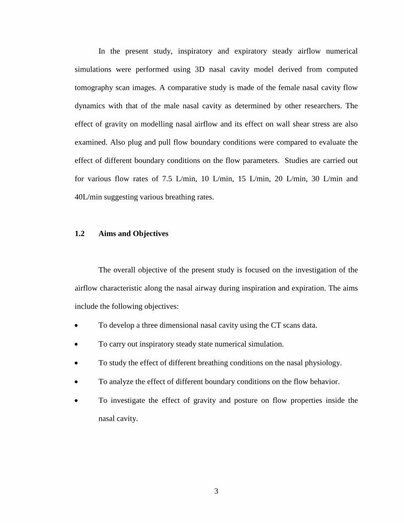
On the lateral wall, there are three horizontal projections called turbinate or
conchae, which divide the nasal cavity into three air passage. The three turbinates are
named as inferior, middle and superior turbinates, according to their position and
function (see Figure 2.2). The airway gap in between the turbinates and the central nasal
septum walls is the meatus. The meatus are very narrow, normally being about 0.5-1mm.
(Proctor and Andersen, 1982). At the posterior end of the main nasal passage, the
turbinates and the septum end at the same point. The point at which the two nasal
cavities merge into one and marks the beginning of the nasopharynx. At this point, the
7
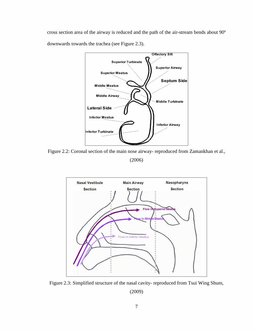
cross section area of the airway is reduced and the path of the air-stream bends about 90º
downwards towards the trachea (see Figure 2.3).
Figure 2.2: Coronal section of the main nose airway- reproduced from Zamankhan et al.,
(2006)
Figure 2.3: Simplified structure of the nasal cavity- reproduced from Tsui Wing Shum,
(2009)
8
2.2.2 Nasal physiology
The human nose has two primary functions. The first is olfaction, the sense of
smell. The second function is air-conditioning. Inspired air is conditioned by a
combination of heating, humidification and filtering to provide the first line protection
for the lung (Elad et al., 2008).
The nasal conchae help to slow down the passage air, causing it to swirl in the
nasal cavity. The nasal cavity is lined by mucous membrane containing microscopic
hairlike structures called cilia. The cells of the membrane produce mucus, a thick gooey
liquid. The mucus moistens the air and traps any bacteria or particles of air pollution.
Microscopic finger-like projections on the surface of the mucosal cells lining the nasal
cavity called cilia. The cilia wave back and forth in rhythmic movement. Cilia will
slowly propel the mucus backwards into the pharynx where it is swallowed. The nose is
so effective that inspired air is cleared of all particulate matter larger than 6 microns-
smaller than the size of a red blood cell.
The nose also acts as the organ of olfaction and has a specially adapted mucosal
lining along its roof for this purpose. In order to stimulate the olfactory system (sense of
smell), the odorant particles must interact with olfactory receptors located in the
olfactory mucosa. Odorants must therefore be capable of being delivered to the olfactory
region by inspired air and be able to dissolve sufficiently in the mucus covering the
olfactory mucosa (Ishikawa et al., 2009).

9
2.3 Objective measurement methods
Objective measurement methods are the conventional tools utilized by medical
practitioners to measure the physiology and anatomy of the nasal cavity. In this section,
the main objective measurement methods are discussed namely rhinomanometry and
acoustic rhinometry.
2.3.1 Rhinomanometry
Rhinomanometry is a tool which is used to measure nasal airway resistance by
making a quantitative measurement of nasal flow and pressure. The European committee
of standardization of Rhinomanometry has selected the formula 𝑅𝑅 = ∆𝑃𝑃/𝑉𝑉 at a fixed
pressure of 150Pa; to facilitate comparison of results. (where 𝑅𝑅=resistance, ∆𝑃𝑃=pressure
drop, 𝑉𝑉 is the velocity of flow). Rhinomanometry can be performed by anterior or
posterior approaches. However this technique is time consuming and requires a great
deal of patient cooperation, particularly difficult with children. It cannot be used in the
presence of septal perforations and when one or both cavities are totally obstructed. It is
affected by nasal cycle and errors as high as 25% are reported for repetitions within 15
minute (Hilberg et al., 1989). It cannot accurately assess a specific area of the nasal
cavity. Rhinomanometry is time consuming, requires technical expertise, a high degree
of subject cooperation and is impossible in subjects with severely congested nasal
airways. There are reports of failure rates of between 25% and 50% in the subjects
examined by rhinomanometry (Austin et al., 1994).

10
2.3.2 Acoustic Rhinometry (AR)
Acoustic Rhinometry analyses ultrasound waves reflected from the nasal cavity
to calculate the cross sectional area at any point in the nasal cavity as well as the nasal
volume. Acoustic rhinometry was first described for clinical use in 1989. The list of
clinical problems that can be analyzed objectively with acoustic rhinometry has
expanded to include turbinoplasty, sleep disorders, more types of
cosmetic/reconstructive procedures, sinus surgery, vasomotor rhinitis, maxillofacial
expansion procedures, and aspirin and methacholine challenge (Corey, 2006). Acoustic
rhinometry is a tool that can aid in the assessment of nasal obstruction. The test is
noninvasive, reliable, convenient, and easy to perform. Common clinical and practical
uses of acoustic rhinometry for the rhinologic surgeon include assessment of “mixed"
nasal blockage, documentation of nasal alar collapse, and preoperative planning for
reduction rhinoplasty.
Acoustic rhinometry can also be used to document the positive effect of surgery
on nasal airway obstruction (Devyani et al., 2004). However, AR may be unreliable due
to artifacts (Tomkinson et al., 1998) & errors can occur in cross sectional area estimation
(Tomkinson et al., 1995). Suzina et al., (2003) concluded that AAR is a sensitive but not
a specific tool for the detection of abnormalities in NAR and it failed to relate to the
symptom of nasal obstruction. There is a poor correlation between subjective sensation
of nasal airflow and objective measurements (Ecckes, 1998). Reichelmann et al., (1999)
found unreliability of acoustic rhinometry in pediatric rhinology. Mean cross-sectional
areas measured by AR were constantly less than those measured by CT of the nasal
cavity up to 33 mm from the nostril, whereas areas measured by AR were greater than
11
those measured by CT scans beyond that point (Min et al., 1995, Mamikoglu et al, 2000).
AR is not a reliable method for the indication or evaluation of surgery for nasal
obstruction (Reber et al., 1998).
2.4 Numerical study of flow through the nasal cavity
Better understanding of airflow characteristic in nasal cavity is essential to study
the physiological and pathological aspect of nasal breathing. The success of nasal
function is highly dependent on the fluid dynamics characteristic of airflow. The
anatomical complexity of the nasal cavity makes direct measurements within the nasal
cavity highly impossible. CFD has the ability to provide quantitative airflow information
at any location within the nasal airway model. These airway models were reconstructed
from magnetic resonance (MRI) or computed tomography (CT) imaging data of patients.
Recent developments in medical imaging coupled with computational science have
opened new possibilities for physically realistic numerical simulations of nasal airflow.
A number of researchers have shown the validity and potential use of CFD in
evaluating the flow conditions inside the nasal cavity. Early work regarding this topic
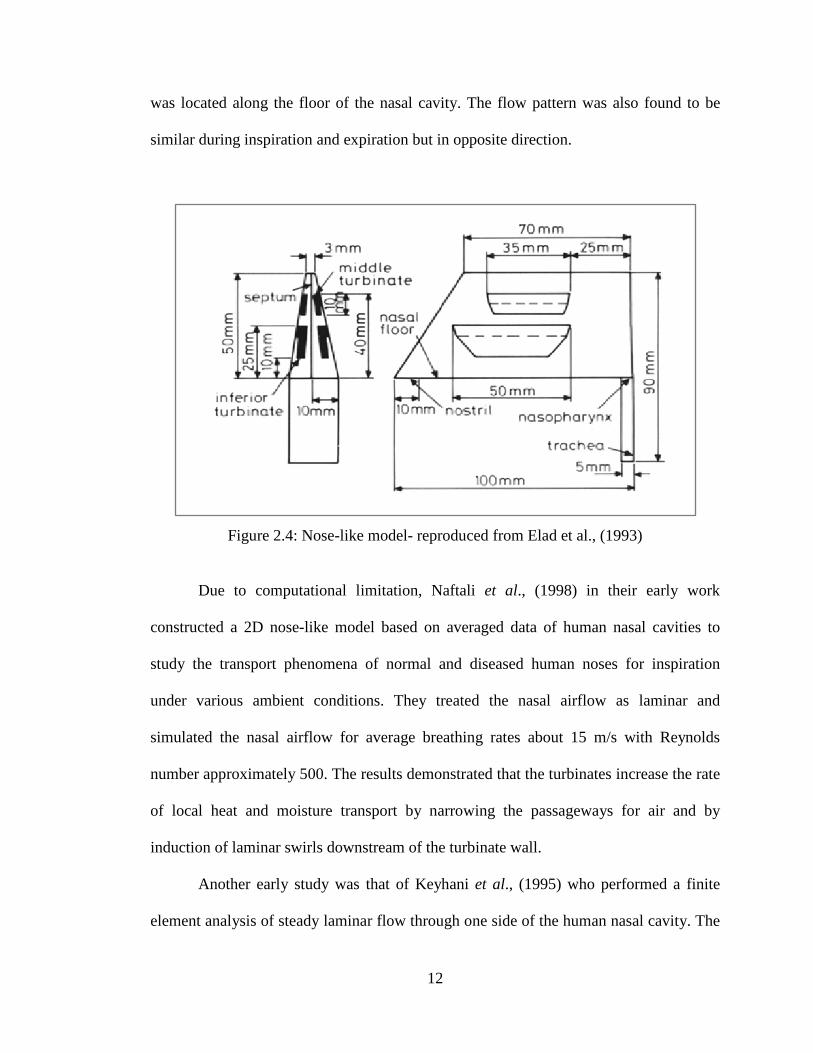
was performed by Elad et al., (1993) who conducted numerical simulations of steady
laminar flow through a simplified nose-like model which resemble the complex anatomy
of human nasal cavity using the finite element software package FIDAP (Fluid
Dynamics International) (see Figure 2.4). The number of mesh created for this nasal
model is approximately <3000 elements. They found that during expiration, flow pattern
spread uniformly into nasal cavity until it reached turbinate. The turbinate is an obstacle
in the airway that increases the resistance to airflow. The lowest resistance in the model
12
was located along the floor of the nasal cavity. The flow pattern was also found to be
similar during inspiration and expiration but in opposite direction.
Figure 2.4: Nose-like model- reproduced from Elad et al., (1993)
Due to computational limitation, Naftali et al., (1998) in their early work
constructed a 2D nose-like model based on averaged data of human nasal cavities to
study the transport phenomena of normal and diseased human noses for inspiration
under various ambient conditions. They treated the nasal airflow as laminar and
simulated the nasal airflow for average breathing rates about 15 m/s with Reynolds
number approximately 500. The results demonstrated that the turbinates increase the rate
of local heat and moisture transport by narrowing the passageways for air and by
induction of laminar swirls downstream of the turbinate wall.
Another early study was that of Keyhani et al., (1995) who performed a finite
element analysis of steady laminar flow through one side of the human nasal cavity. The

13
3D nasal model was reconstructed from 42 coronal CAT scans using an imaging
software called VIDA (Cardiothoratic Imagaing Research Section, University of
Pennsylvania). A computer program was developed in order to convert the coordinate
data into a format that could be processed by the mesh generator module of FIDAP. As
seen in Figure 2.5, the final domain contained 76,950 brick shape mesh elements.
Figure 2.5: Medial slide of the three-dimensional finite element mesh of the right nasal
cavity- reproduced from Keyhani et al., (1995)
The laminar flow was simulated for breathing rates of 125 ml/s and 200 ml/s
using computational fluid dynamics (CFD) software, FIDAP. Their numerical results
were validated with the experimental measurements obtained by Hahn et al., (1993).
According to this study, the majority of the airflow passes through the inferior turbinate.
Results obtained also confirmed that airflow through the nasal cavity is laminar during
quiet breathing.

14
Airflow in the main nasal cavity is generally described as laminar by several
researchers for flow rates of 7.5 L/min to 15 L/min. Segal et al., (2008) performed
numerical simulation of steady state inspiratory laminar airflow for flow rate of 15
L/min. In their study, three dimensional computational models of four different human
nasal cavities which constructed from coronal MRI scans were used (see Figure 2.6).
The nasal model then was meshed with hexahedral elements using a semi-automated
process MAesh which was developed in-house using Matlab (The MathWorks, Inc.,
Natick, MA, USA). In their study, they found that in all four nasal models, the majority
of flow passed through the middle and ventral regions of the nasal passages. The amount
and the location of swirling flow differed among the subjects.
Figure 2.6: Computational meshes for subjects A, 12, 14 and 18. Nostrils are shown in
blue on the right side of the models and the nasopharynx is on the left- reproduced from
Segal et al., (2008)

15
Wen et al., (2008) also simulated steady laminar nasal airflow for flow rates of
7.5 to 15L/min using computational fluid dynamics software FLUENT. An anatomically
correct three dimensional human nasal cavity computed from CT scan images were used
(see Figure 2.7). The solution was found to be mesh-independent at approximately
950,000 cells. Results shows that the nasal resistance value within the first 2-3 cm
contribute up to 50% of the total airway resistance. Vortices were observed in the upper
olfactory region and just after the nasal valve region.
Figure 2.7: Nasal cavity model constructed by Wen et al., (2008)
Inthavong et al., (2007) constructed 3D nasal passage based on nasal geometry
which obtained through a CT scan of a healthy human nose. A constant laminar flow
16
rates about 7.5 L/min was used to simulate light breathing. The mesh in the
computational domain is unstructured tetrahedral and the size of the mesh is
approximately 950,000 cells. The airflow analysis showed vortices present in nasal valve
region which enhanced fibre deposition by trapping and recirculating the fibre in the
regions where the axial velocity is low.
Another work was done by Croce et al., (2006), who also simulated steady state
inspiratory laminar airflow for flow rate of 353 ml/s in both nostril using FLUENT. The
3D computational geometry used in Croce et al., (2006) numerical study was derived
from CT scan images of a plastinated head using a commercial software package,
AMIRA (Mercury Computer System, Berlin). The final adapted mesh consisted of
1,353,795 tetrahedral cells. The results obtained from this study shows that airflow was
predominant in the inferior median part of nasal cavities. Vortices were observed
downstream from the nasal valve and toward the olfactory region.
Other studies include Zamankhan et al., (2006), who study the flow and transport
and deposition of nano-size particle in a three dimensional model of human nasal
passage. The nasal cavity model was contructed from a series of coronal MRI scans.
They simulated the steady state flows for breathing rate of 14 L/min and the Reynolds
number bases on the hydraulic diameter was about 490. The airflow simulation results
were compared with the available experimental data for the nasal passage. They found
that, despite the anatomical differences of the human subjects used in the experiments
and computer model, the simulation results were in qualitatively agreed with the
experimental data.
17
Several researchers treated the nasal airflow as turbulent flow. Liu et al., (2007)
constructed 3D human nose model based on coronal CT scans. A nostril pointing
downwards was added to the nasal geometry model. Unstructured mesh were created
with the size of the mesh was approximately 4,000,000 elements. Turbulent flows were
simulated for inhalation flow rates ranging from 7.5 to 60 L/min by using Reynolds
Averaged Navier-Stokes (RANS)/ Eddy Interaction Model (EIM). Large Eddy
Simulation (LES) modelling was simulated for intermediates flow rates of 30 and 45
L/min. The simulations study showed that the total particle deposition result using LES
indicate that the particle deposition efficiency in the nasal cavity show better agreement
than standard RANS/EIM approach when compared to the in vivo data.
Zhao et al., (2006) also treated the nasal airflow as turbulent in their study. They
constructed 3D nasal model based on CT scans in order to investigate the left nasal valve
airway which was partially obstructed. Then, they modified the nasal valve region
volume to simulate the narrowing of the nasal valve during human sniffing. The airflow
was assumed as turbulent and total nasal flow rates was between 300 and 1000ml/s.
Result from this study revealed that the increase in airflow rate during sniffing can
increase odorant uptake flux to the olfactory mucosa but lower the cumulative total
uptake in the olfactory region when the inspired air/odorant volume was held fixed.
Another nasal airflow analysis using the turbulence model was conducted by
Mylavarapu et al., (2009). They investigated the fluid flow through human nasal airway
model which was constructed from axial CT scans. TGRID was then used to create an
unstructured hybrid volume mesh with approximately 550,000 cells. Flow simulations
and experiments were performed for flow rate of 200 L/min during expiration. Several
different numerical approaches within the FLUENT commercial software framework

18
were used in the simulations; unsteady Large Eddy Simulation (LES), steady Reynolds-
Averaged Navier-Stokes (RANS) with two-equation turbulence models (i.e. k-epsilon,
standard k-omega, and k-omega Shear Stress Transport (SST)) and with one-equation
Spalart-Allmaras model. Among all the approaches, standard k-omega turbulence model
resulted in the best agreement with the static pressure measurements, with an average
error of approximately 20% over all ports. The largest pressure drop was observed at the
tip of the soft palate. This location has the smallest cross section of the airway.
Numerical study on human nasal airflow with abnormal nasal cavity cause by
several chronic diseases also has been the subject of several studies. Wexler et al.,
(2005) constructed 3D nasal model of a patient with sinonasal disease. They investigated
the aerodynamic consequences of conservative unilateral inferior turbinate reduction
using computational fluid dynamics (CFD) methods to accomplish detailed nasal airflow
simulations. Steady-state, inspiratory laminar airflow simulations were conducted at
15L/min. They found that inferior turbinate reduce the pressure along the nasal airway.
Also, the airflow was minimally affected in the nasal valve region, increased in the
lower portion of the middle and posterior nose, and decreased dorsally.
Garcia et al., (2007) constructed 3D nasal geometry by using medical imaging
software (MIMICs, Materialise) to investigate airflow, water transport, and heat transfer
in the nose of an Atrophic Rhinitis (AR). The patient underwent a nasal cavity-
narrowing procedure. Rib cartilage was implanted under the mucosa along the floor of
the nose, and septum spur was removed. The reconstructed nose was simulated and the
nasal airflow was assumed as laminar with 15 L/min corresponding to resting breathing
rate. This study showed that the atrophic nose geometry had a much lower surface area

19
than the healthy nasal passages. The simulations indicated that the atrophic nose did not
condition inspired air as effectively as the healthy geometries.
Lindemann et al., (2005) produced 3D model of human nose to investigate the
intranasal airflow after radical sinus surgery. The human nasal model was constructed
based on CT scans of the nasal cavities and the paranasal sinuses of an adult. The
numerical simulation was performed by assuming the nasal airflow as laminar at 14
L/min for quiet breathing rate. Result showed that aggressive sinus surgery with
resection of the lateral nasal wall complex and the turbinates cause disturbance of the
physiological airflow, an enlargement of the nasal cavity volume, as well as an increase
in the ratio between nasal cavity volume and surface area.
2.5 Gender comparison
Several researchers have shown the benefits of computational fluid dynamics
(CFD) in better understanding of flow through the nasal cavity. Some of the main
players are Wen et al., (2008), Mylavarapu et al., (2009), Segal et al., (2008), Weinhold
et al., (2004), Xiong et al., (2008). However, most of the researchers employed male
human subject in the determination of the nasal patency. Inter human anatomical
differences exists and also differences on anatomical and physiological morphology are
observed based on gender. No specific numerical modelling studies have been carried
out to compare and ascertain the effect of gender on flow variable inside the nasal
cavity. Gender differences is said to be the important determinant of clinical
manifestations of airway disease. Even though obstructive sleep apnea, is prevalent in
both the gender, its effect on male subjects is more prominently observed (Rowley et al.,
20
2002). Also a higher prevalence of irregular breathing phenomenon among men when
compared to women during sleeping and also the fact that men have a larger upper
airways in sitting and supine positions (Thurnheer et al., 2001) makes it all the more
important to study the effect of gender on breathing phenomenon. It would be an
importance too to study the effect of anatomical variation based on gender on the flow
parameter.
2.6 Gravity Effect
Also CFD modelling involves various simplifications, for example the postural
effects which drastically affect the outcome of the analysis. The postural changes in
nasal airway resistances are of clinical importance when accessing patients with nasal
obstruction. Mohsenin, (2003) demonstrated the effect of decrease in pharyngeal cross
sectional area and occurrence of OSA. The gravitational force is considered to be one
significant determinant of the closing pressure (Watanabe et al., 2002). Study performed
by Tvinnereim et al., (1996) showed that nasal and pharyngeal resistance doubles upon
assumption of supine posture; however the difference obtained was not statistically
significant. Beaumont et al., (1998) found that at sea level, gravity forces that cause the
soft palate and tongue to fall back in the supine posture would narrow upper airways in
all its length. A study by Hsing-won Wang, (2002) on the effect of posture on nasal
resistance varied from 0.612 Pa/mL/sec in sitting position to 0.663Pa/mL/sec in the
supine position.

21
Matsuzawa et al., (1995) observed that the MRI data obtained in supine, lateral
and prone position revealed that the upper airway was narrowest in the supine position,
and widest in the prone position indicating the anatomical narrowing of the upper airway
especially the pharyngeal area. Martin et al., (1995) showed in the supine position all the
upper airway dimensions decreases with increasing age in both men and women, except
the oropharyngeal junction. Hence, it is very important to study the effect of gravity on
the flow through the nasal cavity.
2.7 Plug flow and pull flow boundary condition
Keyhani et al., (1995), Wexler et al., (2005), Zamankhan et al., (2006), Segal et
al., (2008), and Ishikawa et al., (2009) constructed 3D nasal computational models and
simulated the airflow by utilizing plug flow boundary condition. For plug flow, fixed
airflow rate with a uniform velocity profile was imposed at the nostril. While a stress
free boundary condition was used at the outflow boundary condition. On the other hand,
the pull flow boundary condition is based on negative pressure set at the nasopharynx.
Garcia et al., (2007) used pull flow boundary condition to study the airflow and water
transport simulation in the nasal cavity. Wexler et al., (2005) also attempted to conduct
the nasal airflow simulation using pull flow boundary condition. However, this
simulation has been unsuccessful due to the failure of residuals to converge. There is still
no unanimity among the researchers with respect to the use of exact boundary
conditions. Most researchers employed the plug flow model in order to stimulate the
flow features inside the nasal cavity. The natural physiological inspiratory mechanism is
based on pull flow conditions, wherein the expansion of the lungs sets in negative

22
pressure gradient enabling the air from the ambient atmosphere to rush inside the nasal
cavity through the nostril inlets.
2.8 Summary
In summary, the literature reviewed shows that all the previous numerical studies
on nasal airflow have generalized the behavior to both gender. No specific numerical
modelling studies have been carried out to compare and ascertain the effect of gender on
flow variable inside the nasal cavity. Also CFD modelling involves various
simplifications, for example the postural effects which drastically affect the outcome of
the analysis. It was also found that there is no unanimity with respect to the use of exact
boundary conditions. Hence there is no standardization of the boundary definition with
respect to the study concerning the nasal flow using numerical methods. Therefore the
current work will investigate the effect of different boundary condition on nasal airflow
behavior through the human nasal cavity. Also the effects of gravity and posture on flow
properties inside the nasal cavity will be investigated. Finally, the gender effect on nasal
airflow characteristic due to variation in nasal anatomy will be studied.

23
CHAPTER 3
METHODOLOGY
3.1 Overview
This chapter presents the method used to reconstruct the three-dimensional
model of the human nasal cavity, mesh generation and numerical setup for the nasal
airflow simulation. The overall process of the present numerical study has been
illustrated in the flow chart below.
Convert 2D CT scan images to 3D CAD data using MIMICS
Geometry Creation using CATIA
Mesh Generation using GAMBIT
CASE SETUP
PRE-PROCESSING
Different breathing rate - Comparison
Comparison of plug and pull flow Gravity effect
POST-PROCESSING
Results and Analysis
DISCUSSION AND CONCLUSIONS
Procuring CT scan data of human nasal cavity
FLUENT simulation setup
Grid Independence Test

24
3.2 3D computational model of the nasal cavity
Reconstruction of 3D anatomical model of the human nasal cavity can be very
time consuming. The general process of developing the 3D anatomical model basically
consist of selection of CT scan data of human nasal cavity followed by converting the
2D CT scan images into 3D CAD data using medical image processing software,
MIMICs and finally construct the surface geometry by using CAD software, CATIA.
3.2.1 Procuring CT scan data of human nasal cavity
The anatomical model of the nasal airway used for this numerical study was
derived from CT scan images of a healthy 39 year old Malaysian female. The CT scan
image of the nasal airway was taken from pre-existing CT scan data sourced from
Universiti Sains Malaysia, Medical Campus Hospital. The nasal anatomy was attested
to be normal by the ear, nose and throat (ENT) surgeon. Figure 3.1 shows a series of
coronal CT scan images along the axial distance of the nasal cavity of the female human
subject. The scans produced a total 385 slices of axial, coronal and sagittal images which
accounted for the complete nasal cavity area, from nostril to nasopharynx.
The increment between each slice of the scan images is 0.8mm and the scan pixel
resolution is 0.434mm. It is important to make sure that the scan interval is less than 2
mm in order to accurately capture the complex geometry of the nasal cavity and to avoid
stair-step artifact which usually appear on the curved surface of the model (Bailie et al.,
2006). However, reduction of the layer thickness requires more expensive machines and
a slower build process. The CT scan data was imported into medical image processing

25
software MIMICs for the reconstruction of the 3D human nasal cavity for this case
study.
Figure 3.1: Coronal CT scan images along the axial distance of the human nasal cavity
3.2.2 Convert 2D CT scan images to 3D CAD data using MIMICs
MIMICs is an image processing and editing software which provides the tool for
the visualization and segmentation of CT images and also for the 3D rendering of
objects. Before the scan data can be processed, MIMICs reads the 2D CT scan images
from the DICOM (*.dcm) file format and convert it into MIMICs (*.mcs) file format.
26
MIMICS will compress and merge all the axial, coronal and sagittal scan images into a
single volume file project based on the similar pixel size value.
Figure 3.2: CT scan images from A: axial, B: coronal and C: sagittal plane and 3D
model of the female human nasal cavity
The main step of nasal geometry reconstruction from the CT scan data is the
segmentation process in which the regions of interest, nasal passage is identified. The
segmentation was developed based on the Hounsfield Units (HU) in the CT images. HU
is a measure of the electron density of the tissue. Segmentation was performed by
defining a range of threshold values to create the segmentation mask. The range of the
threshold value used for this case study is between -444 to 2037 HU (see Figure 3.2). A
correct threshold value is vital in capturing the important features of the nasal cavity.
The threshold value is used to differentiate between bone and soft tissues and to
A B
C
27
determine the set of structures to be included in the 3D nasal model. Medical
reconstruction requires a good understanding of anatomy, which can only come with
experience, and understanding the types of tissue that are preferentially imaged by
radiographers. Hence the presence of an expert radiologist and ENT practitioner is
essential in deciding the threshold and editing of the geometry.
An automatic region growing function was used to reconstruct the nasal airway
from the nostril to nasopharynx based on the segmented mask. The purpose of the region
growing function was to reduce the noise, remove floating pixels and to split the
unconnected structure. However, manual segmentation is also required to edit the mask
which leak to surrounding region and remove the unwanted parts which are still
connected to the nasal cavity model. Manual editing function also makes it possible to
draw and restore parts of image on the segmented mask. By using the MIMICs editing
tools, the scan images were segmented slice by slice on axial, coronal and sagittal plane
by using the local threshold value.
MIMICs has the ability to generate and display the 3D anatomical model of the
nasal cavity from the segmented scan images. After all the necessary threshold editing,
the 3D anatomical model of the nasal cavity was generated from the segmented mask.
By using the 3D rendering tools, the 3D nasal cavity model was examined to ensure the
suitability of the selected threshold and to confirm the presence of all the required
structure for the physical anatomical model.
MIMICs also provide the export function which can be use to export the 3D
object produced from the segmented CT scan images into IGES file and can be directly
used in any CAD system. As seen in Figure 3.3, the polylines was created based on the
segmented mask of the 3D object on each slice of the project by using ‘calculate polyline

28
function’. Later the 3D polylines data was exported as IGES (*.igs) file format, for the
surface model generation using the CAD software, CATIA.
Figure 3.3: Polyline data of the 3D human nasal cavity
3.2.3 Geometry creation using CATIA
The coordinates of the contour point extracted from the CT scan data of the
human nasal cavity was imported into CAD software package, CATIA using Digitized
Shape Editor (DSE) workbench for surface model generation. DSE is usually used at the
initial stages of the reverse engineering and it also provides tools for various operations
on the imported digitized data. The IGES (*.igs) file can be imported and displayed in
DSE workbench in the form of cloud of points or polylines. However, due to anatomical

29
complexity, it is not possible to edit and manipulate the 3D anatomical model in the
cloud of points form.
Therefore, facets were created directly from the polylines which is as shown is
Figure 3.4a using the mesh creation tools. The neighborhood parameter value was set to
7.5mm to define the maximum length of the facet edge. The function of the
neighborhood value is to close the unwanted holes of the mesh. Increasing the
neighborhood parameter will lead to a non manifold mesh. After the mesh surfaces have
been created from the polylines, the next stage is to edit the 3D nasal mesh geometry by
removing the unwanted mesh part. As seen in Figure 3.4d, all the paranasal sinuses have
been removed in order to simplify the geometry and to reduce the computational cost.
Editing was carefully carried out to preserve the original shape of the anatomical model
of the human nasal cavity (see Figure 3.4e).
By using the cleaning mesh function, the defective mesh was removed to
improve the quality of the mesh. The mesh cleaner helped analyze and delete all the
defective mess which consisted of non manifold edges, non manifold vertices, isolated
triangle, triangle with inconsistent orientations and the corrupted triangles. After all the
necessary mesh cleaning, the 3D mesh geometry was smoothened using the mesh
smoothing tool to improve mesh surface quality. Finally, the 3D computational model of
the human nasal cavity was created based on the smooth mesh surface by using the
automatic surface tool in Quick Surface Reconstruction workbench. Figure 3.4f shows
the final 3D model of the nasal cavity obtained from CATIA which can be used for
computational modelling.

30
a) Polyline data
f) The final 3D reconstructed model of the
nasal cavity
b) Surface mesh generation
e) Smoothing operation
c) Nasal cavity with paranasal sinuses
d) Nasal cavity with paranasal sinuses
removed
Figure 3.4: Steps involved in developing 3D model of the nasal cavity using CATIA
31
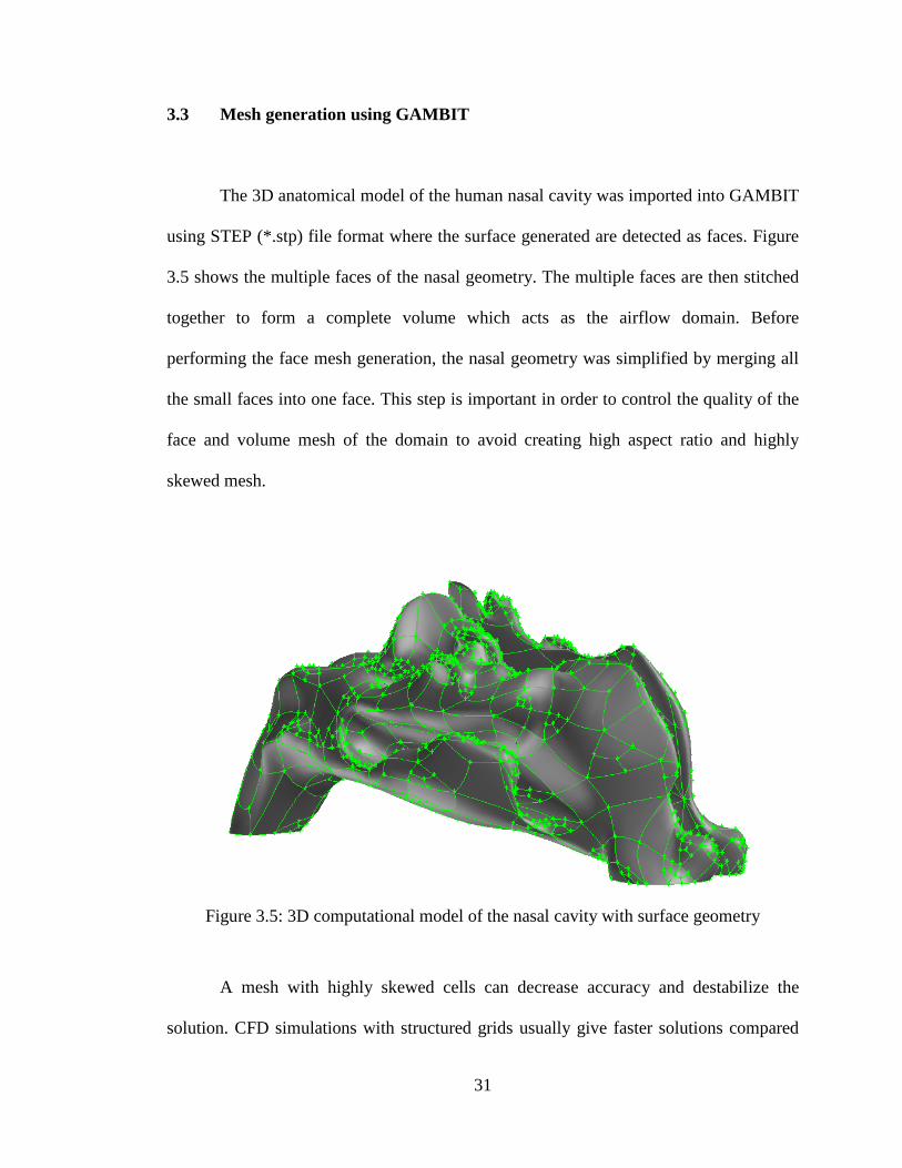
3.3 Mesh generation using GAMBIT
The 3D anatomical model of the human nasal cavity was imported into GAMBIT
using STEP (*.stp) file format where the surface generated are detected as faces. Figure
3.5 shows the multiple faces of the nasal geometry. The multiple faces are then stitched
together to form a complete volume which acts as the airflow domain. Before
performing the face mesh generation, the nasal geometry was simplified by merging all
the small faces into one face. This step is important in order to control the quality of the
face and volume mesh of the domain to avoid creating high aspect ratio and highly
skewed mesh.
Figure 3.5: 3D computational model of the nasal cavity with surface geometry
A mesh with highly skewed cells can decrease accuracy and destabilize the
solution. CFD simulations with structured grids usually give faster solutions compared

32
to unstructured grids. However, in the present case, due to the anatomical complex
structure of the human nasal cavity, it is not only time consuming but almost impossible
to create structured grids. Hence, unstructured mesh consisting of tetrahedral elements is
preferred for developing the mesh.
Figure 3.6: Volume mesh of the 3D computational model of human nasal cavity
The accuracy of the CFD study depends primarily on quality and quantity of the
mesh distribution. An initial model with 106,393 cells was created and used to solve the
airflow field at a flow rate of 7.5L/min. The schematic diagram of the grid is show in the
Figure 3.6. The grid independency test was carried out using the gradient adaptation
technique. The original mesh was refined based on the velocity gradient. This process
was repeated, with each repetition produce a model with a higher cell count than the
previous model.
The grid independence test resulted in an optimized grid with 577,010 elements.
This was considered sufficient taking into account the computational time and system
INLET: NOSTRIL
WALL
OUTLET: NASOPHARYNX
33
memory. Variation in pressure and velocity with higher grid were negligible. Hence, the
mesh with 577,010 elements was used for our simulation. In order to ensure the accuracy
of the flow simulation near the wall surfaces, the y+ values obtained for the nasal cavity
model is less than 5. The wall y+ value is the distance between the cell centroid to the
wall for wall-adjacent cell.
𝑦𝑦+ = 𝑢𝑢𝜏𝜏𝑦𝑦𝑣𝑣
(3.1)
Where y is the normal distance of the first grid point from the wall, 𝑢𝑢𝜏𝜏 is the friction
velocity and 𝑣𝑣 is the kinematic velocity of the fluid flow.
3.4 Numerical analysis
This sub-chapter provides the governing equations for the current fluid flow
problem and numerical models used for the numerical simulation.
3.4.1 Governing equation
CFD is fundamentally based on the governing equations of fluid dynamics. They
represent mathematical statements of the conservation laws of physics. For a general
fluid property defined by Ф, can be cast into transport equation form as:
𝜕𝜕(𝜌𝜌Ф)𝜕𝜕𝜕𝜕
+ 𝑑𝑑𝑑𝑑𝑣𝑣(𝜌𝜌Ф𝒖𝒖) = 𝑑𝑑𝑑𝑑𝑣𝑣(Г𝑔𝑔𝑔𝑔𝑔𝑔𝑑𝑑Ф) + 𝑆𝑆Ф (3.2)

34
The first and second terms on the left are time derivative term and the convective terms.
The terms on the right are the diffusive terms and the source terms. In words, equation
above can be read as:
Rate of increase
of Ф in a fluid
element
+
Net rate of flow
of Ф through a
fluid element
=
Rate of increase
of Ф due to
diffusion
+
Rate of increase
of Ф due to
additional sources
The governing equation of fluid flow for an incompressible fluid, such as the airflow in
the respiratory system can be written as:
𝜕𝜕Ф𝜕𝜕𝜕𝜕
+ 𝜕𝜕(𝑢𝑢Ф)𝜕𝜕𝜕𝜕
+ 𝜕𝜕(𝑣𝑣Ф)𝜕𝜕𝑦𝑦
+ 𝜕𝜕(𝑤𝑤Ф)𝜕𝜕𝜕𝜕
= 𝜕𝜕𝜕𝜕𝜕𝜕�Г 𝜕𝜕Ф
𝜕𝜕𝜕𝜕� + 𝜕𝜕
𝜕𝜕𝑦𝑦�Г 𝜕𝜕Ф
𝜕𝜕𝑦𝑦� + 𝜕𝜕
𝜕𝜕𝜕𝜕�Г 𝜕𝜕Ф
𝜕𝜕𝜕𝜕� + 𝑆𝑆Ф (3.3)
Where t is time, u, v, w represent velocity components, Г is the diffusion coefficient, and
𝑆𝑆Ф is a general source term. This equation is commonly used as the starting point for
computational procedures in the finite volume method.
3.4.2 Turbulence models
In the current study, the simulation is based on the numerical solution of the
Reynolds Averaged Navier-Stokes equation representing the general equation for 3D
flow of incompressible and viscous fluids. The SST k-ω turbulence model, a two
equation turbulence model was employed. The SST k- ω model accounts for transport of
35
turbulent shear stress and gives highly accurate predictions of the amount of flow
separation under adverse pressure gradient.
The SST model is a blend between the k-𝜔𝜔 turbulence model, which is applicable
near the walls, and the k-𝜀𝜀 turbulence model which is applied at the core of the
computational domain, with an additional limiter in the formulation of the eddy viscosity
to provide proper account of the turbulent SST. Therefore SST combines the advantages
of both the k-𝜀𝜀 and k-𝜔𝜔 methods. The k-𝜔𝜔 turbulence model has a near wall treatment
allowing accumulation of nodes towards the wall without any special non-linear
damping function, whereas the k-𝜀𝜀 model is less sensitive to free stream and inlet
conditions.
The combination is ideal for a flow in a complex geometry like the nasal cavity
(Liu et al., 2007). The suitability of SST k-ω model also has been experimentally
validated by Mylavarapu et al., (2009), Ahmad et al., (2010) and Zubair et al., (2010).
3.4.3 Numerical solver procedure
The governing transport equations were discretized using the control volume
based technique. The domain is discretized into control volumes based on the created
computational mesh. The governing equations were converted into integral form to
allow integration of the equation on each computational mesh. A set of algebraic
equations for dependent variables such as velocities, pressure and temperature are then
set up and solved.

36
The segregated pressure based solver within FLUENT was chosen which solved
the governing equations. Figure 3.7 shows the flow chart of the iteration procedure based
on the segregated pressure-based solution method. FLUENT stores discrete values of the
scalar Ф at the cell center. However, face values Фf required for convection terms and
must be interpolated from the cell center values. This is accomplished by using an
upwind scheme.
Figure 3.7: Pressure-based solution method (FLUENT User manual)
In the present study, first order upwind scheme was used initially to stabilize the
flow. Smaller under relaxation factors value was applied in order to gain flow stability.
After the first order converged, the second order upwind scheme was then utilized to
Update properties
Solve sequentially: Uvel, Vvel, Wvel
Solve pressure-correction (continuity) equation
Update mass flux, pressure, and velocity
Solve energy, species, turbulence, and other scalar equations
Converged Stop Yes No

37
accomplish higher order accuracy of the flow solution. The quality of the second order
upwind scheme has been proved for its reliability and accuracy in evaluating the scalar
variables on unstructured meshes (FLUENT User manual).
The SIMPLE algorithm was used to obtain the relationship between velocity and
pressure corrections to enforce mass conservation and also to obtain the pressure.
Convergence was considered complete only when the residuals for all equations dropped
by six order of magnitude (10-6) and when the residuals had flat-lined.
3.4.4 Boundary condition definition
The boundary conditions are defined in Table 3.1. The nasal wall was assumed to
be rigid and the simulation ignored the presence of mucus. A no-slip boundary condition
was defined at the walls. For plug flow inspiration case, mass flow rate was imposed at
the nostril inlet and outflow boundary was defined at the nasopharynx outlet. Since, the
velocity or pressure at the nasopharynx are not known prior to solution of the flow
problem, we used outflow boundary condition to model the nasopharynx exit during
inspiration. Expiration for plug flow was defined as pressure outlet at the nostril and
mass flow rate at the nasopharynx.
Table 3.1: Boundary condition for pull flow and plug flow
Inspiration Expiration
PLUG FLOW Inlet Mass flow inlet Pressure outlet
Outlet Outflow Mass flow inlet
PULL FLOW Inlet Inlet Pressure Pressure outlet
Outlet Pressure outlet Pressure inlet

38
The pull flow inspiration model was simulated using negative pressure value set
at the nasopharynx and pressure inlet with athmospheric pressure equivalent of 0 Pa was
adopted at nostrils accounting for the desired mass flow rate. An expiration case was
simulated using pressure outlet at the nostril and positive pressure value defined at
nasopharynx. The pressure gradient was selected so as to maintain the required mass
flow rate entering the system.
Steady state laminar and turbulent airflow simulations were modelled. At
15L/min the Reynolds number obtained at the nostril inlet was around 1,600 and for
20L/min the Reynolds number was 3,100. The airflow was therefore laminar for flow
rates up to 15L/min and the flow was treated as turbulent flow beyond 15L/min. This
was also in general agreement with previous researchers (Wen et al., 2008, Segal et al.,
2008), who determined laminar nature of the flow, for flow less than 15 L/min.
In turbulent flow computations, additional boundary conditions for turbulence
parameters need to be specified at inlet locations. Turbulent intensity at the nostril inlet
was set to 5%, and the viscosity ratio value is 10 (Liu et al., 2007). The simulation was
carried out on an IBM platform, Intel, Xenon(R) CPU, 2GB RAM which typically took
nearly to 2 days to complete the simulation.
39
CHAPTER 4
RESULTS AND DISCUSSION
4.1 Overview
This chapter presents and discusses the results obtained from the numerical
simulation of the human nasal cavity. Each of the cases studied are presented as different
subchapters. The case study includes the basic understanding of the nasal physiology,
comparison between different flow rates for both inspiration and expiration, effect of
gender based anatomical variations on the nasal airflow, gravity effect and boundary
condition prescription for nasal airflow simulation.
4.2 Grid dependency analysis
A grid dependency study has been performed for the nasal cavity computational
model. The model was initially developed using unstructured tetrahedral mesh with
106,393 numbers of elements. Gradient adaptation was performed based on the average
velocity values obtained from the nasal airflow simulation during inspiration for flow
rates of 7.5 L/min. As seen in Figure 4.1, the grid independence test has been conducted
in the same nasal cavity model with different size of mesh. Each adaptation resulted in a
new mesh and the variation in velocity parameter was noted for different locations till
the variations were negligibly small.

40
Figure 4.1: Grid independence plot
The results obtained shows that the average velocity values do not change as the
mesh resolution increased to 591878. Hence, the mesh with 577010 elements was used
for our simulation. This was considered sufficient taking into account the computational
time and system memory. Near wall model approach was applied, where the mesh close
to the wall was refined in order to resolve the near wall flow for turbulent airflow. In
order to ensure the accuracy of the flow simulation near the wall surfaces, the y+ values
obtained for the nasal cavity model is less than 5.
0
0.5
1
1.5
2
2.5
3
0 2 4 6 8 10
Ave
rage
Vel
ocit
y (m
/s)
Axial Distance (mm)
360829573923574980575218577010
41
4.3 Geometry comparison
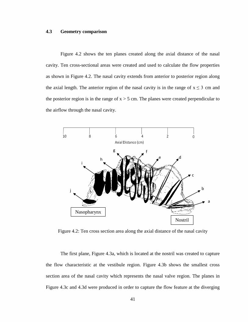
Figure 4.2 shows the ten planes created along the axial distance of the nasal
cavity. Ten cross-sectional areas were created and used to calculate the flow properties
as shown in Figure 4.2. The nasal cavity extends from anterior to posterior region along
the axial length. The anterior region of the nasal cavity is in the range of x ≤ 3 cm and
the posterior region is in the range of x > 5 cm. The planes were created perpendicular to
the airflow through the nasal cavity.
Figure 4.2: Ten cross section area along the axial distance of the nasal cavity
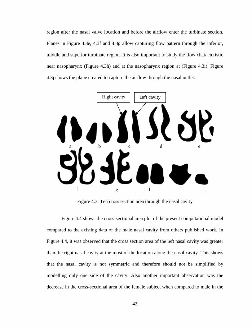
The first plane, Figure 4.3a, which is located at the nostril was created to capture
the flow characteristic at the vestibule region. Figure 4.3b shows the smallest cross
section area of the nasal cavity which represents the nasal valve region. The planes in
Figure 4.3c and 4.3d were produced in order to capture the flow feature at the diverging
Nostril
Nasopharynx
a
f e d
c
b
i h
g
j
42
region after the nasal valve location and before the airflow enter the turbinate section.
Planes in Figure 4.3e, 4.3f and 4.3g allow capturing flow pattern through the inferior,
middle and superior turbinate region. It is also important to study the flow characteristic
near nasopharynx (Figure 4.3h) and at the nasopharynx region at (Figure 4.3i). Figure
4.3j shows the plane created to capture the airflow through the nasal outlet.
Figure 4.3: Ten cross section area through the nasal cavity
Figure 4.4 shows the cross-sectional area plot of the present computational model
compared to the existing data of the male nasal cavity from others published work. In
Figure 4.4, it was observed that the cross section area of the left nasal cavity was greater
than the right nasal cavity at the most of the location along the nasal cavity. This shows
that the nasal cavity is not symmetric and therefore should not be simplified by
modelling only one side of the cavity. Also another important observation was the
decrease in the cross-sectional area of the female subject when compared to male in the
a b c d e
f g h i j
Left cavity Right cavity
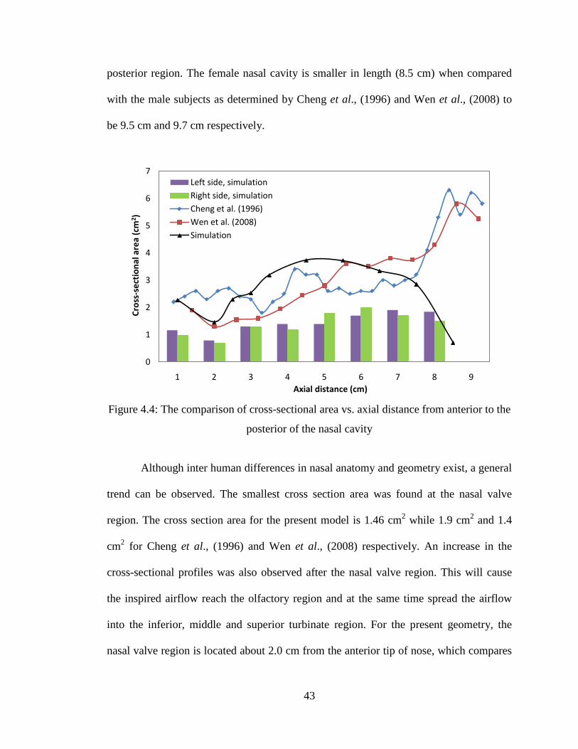
43
posterior region. The female nasal cavity is smaller in length (8.5 cm) when compared
with the male subjects as determined by Cheng et al., (1996) and Wen et al., (2008) to
be 9.5 cm and 9.7 cm respectively.
Figure 4.4: The comparison of cross-sectional area vs. axial distance from anterior to the
posterior of the nasal cavity
Although inter human differences in nasal anatomy and geometry exist, a general
trend can be observed. The smallest cross section area was found at the nasal valve
region. The cross section area for the present model is 1.46 cm2 while 1.9 cm2 and 1.4
cm2 for Cheng et al., (1996) and Wen et al., (2008) respectively. An increase in the
cross-sectional profiles was also observed after the nasal valve region. This will cause
the inspired airflow reach the olfactory region and at the same time spread the airflow
into the inferior, middle and superior turbinate region. For the present geometry, the
nasal valve region is located about 2.0 cm from the anterior tip of nose, which compares
0
1
2
3
4
5
6
7
1 2 3 4 5 6 7 8 9
Cros
s-se
ctio
nal a
rea
(cm
2 )
Axial distance (cm)
Left side, simulationRight side, simulationCheng et al. (1996)Wen et al. (2008)Simulation

44
with the other models that are located at 3.3 cm and 2.0 cm for Cheng et al., (1996) and
Wen et al., (2008) respectively.
4.4 Model comparison
Figure 4.5 shows the nasal resistance plot for various flow rate obtained from the
present computational model compared with the existing data available. The average
pressure drop between the nostril and nasopharynx was obtained at flow rates from
7.5L/min to 40 L/min. A laminar model for the flow rates 7.5 to 15 L/min and the SST
k-ω turbulent model for the flow rates 20 to 40L/min were used to simulate the flow
fields. For the laminar flow rates (<15 L/min) the slope of the impedance curve for our
simulation is almost the same as found by other researchers. However, as flow rate
increases, turbulence plays a significant role, the impedance curve start to depart from
each other as seen in Figure 4.5.
From the observation, the nasal resistance in the case of female model also
follows the same pattern as that of the male subject. However the slope of the resistance
curves as seen in Figure 4.5 is steeper in case of the female subject. This may be
attributed to the anatomical differences; female model is shorter in length and has
smaller posterior cross sectional area. At low velocity, the flow is laminar. It was
observed that the flow is smooth and properly arranged. Hence, the nasal area is not the
critical factor that determines the pressure drop. But when the flow is turbulent, it
consists of chaotic, highly disordered flow and also exhibit higher flow speed. Hence the
nasal area plays an important role and also results in recirculation and reverse flow.
Furthermore, incomparison to the male models, the current female model exhibited

45
smaller cross sectional area at the nasopharynx. This is also the reason for the current
female model to have higher value of pressure drop.
Figure 4.5: Pressure drop vs. inspiratory flow rates compared with previous data
The pressure drop obtained for the female nasal cavity was around 22.6 Pa for 20
L/min when compared with male model at around 18 Pa & 20 Pa for the same flow rate
as obtained by Wen et al., (2008) and Weinhold et al., (2004) respectively. Hence, in
spite of the anatomical differences a close resemblance of result can be seen with the
respect to the previous studies, thereby validating of our present study.
0
10
20
30
40
50
60
70
80
90
0 5 10 15 20 25 30 35 40 45
Pres
sure
Dro
p (P
a)
Flow Rate (L/min)
Wen et al. (2008)
Weinhold et al. (2004)
Simulation

46
4.5 Basic flow studies
Understanding the properties of airflow in the nasal cavity is very important in
determining the nasal physiology and in diagnosis of various anomalies associated with
the nose. However, the conventional methods like rhinomanometer and acoustic
rhinometry fail to accurately predict and quantify the flow properties at every location
inside the nasal cavity. Airflow simulations based on computational fluid dynamics is
most useful for better understanding of flow phenomenon inside the nasal cavity. Hence,
in the present study, the numerical simulation of nasal airflow was performed in order to
obtained details of flow characteristic along the nasal cavity. This chapter present the
results obtained from numerical study of nasal airflow for 20 L/min during inspiration.
4.5.1 Reynolds number calculation
The Reynolds number usually is used to characterize the type of the flow,
whether the flow is laminar or turbulent. Reynolds number is a dimensionless number
which also present the ratio of inertial forces to viscous forces acting on a fluid element.
Reynolds numbers of the nasal airflow can be obtained from:
𝑅𝑅𝑅𝑅 = 𝜌𝜌𝜌𝜌𝜌𝜌𝜇𝜇
(4.1)
Where 𝜌𝜌 the air density (1.225 𝑘𝑘𝑘𝑘/𝑚𝑚3), u is the airflow velocity, d is the diameter of the
nasal inlet and 𝜇𝜇 is the dynamic viscosity of the air (1.7894 × 10⁻⁵ 𝑘𝑘𝑘𝑘/𝑚𝑚𝑚𝑚). The initial
prediction of the Reynolds number value is important in order to properly simulate the
nasal airflow. The flow will be defined as laminar for 𝑅𝑅𝑅𝑅 < 2100 and turbulent for 𝑅𝑅𝑅𝑅 >
47
2100. In the present work, numerical simulation were carried out for flow rates of 7.5
L/min, 10 L/min, 15 L/min, 20 L/min, 30 L/min and 40 L/min. The Reynolds number
value for flow rates of 1 5L/min calculated from the equation above is 1,597. Based on
the Reynolds number obtained, the airflow was treated as laminar for flow rates up to 15
L/min. This was in general agreement with previous researchers (Wen et al., 2008; Segal
et al., 2008) who determined laminar nature of the flow, for flow less than 15 L/min.
The Reynolds number obtained for 20 L/min based on the equation above is
approximately equal to 2,129. Hence, the flow was treated as turbulent for flow rates of
20 L/min and above.
4.5.2 Velocity
Figure 4.6 shows the contour plot of the average velocity value along the nasal
cavity during inspiration. As seen in Figure 4.6, the flow was observed to be fully
developed along the middle meatus region. The superior and inferior meatus pathway
received lesser flow. Low velocity value was also observed at the inferior and superior
turbinate regions. As seen in Figure 4.6 and 4.7, sudden increase of average velocity
value was noticed at the nasopharynx region. This is due to decrease in cross section
area at the posterior region of the nasal geometry.

48
Figure 4.6: Average velocity contour along the nasal cavity
As seen in Figure 4.7, the nasal valve located at a distance of around 2cm from
the anterior region of the nasal cavity. The maximum velocity attained at the nasal valve
location varies from 4.18 m/s as against 4.82 m/s & 3.1 m/s obtained by Xiong et al.,
2008 and Croce et al., 2006 respectively. The peak airspeed in each plane decreases
posteriorly beyond nasal valve region as the cross sectional area increase.
Figure 4.8 shows the streamline plot of the inspired nasal flow through the
nostril. As seen in Figure 4.8, the low velocity re-circulating stream was found just
posterior to the nasal valve region. The re-circulatory flow propagates the flow to the
olfactory region thus making contact with the olfactory sensor. The aerodynamic shape
of the nasal cavity facilitates the re-circulatory flow caused by adverse pressure gradient
due to sudden increase in cross section area after the nasal valve region.
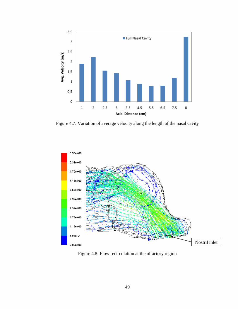
49
Figure 4.7: Variation of average velocity along the length of the nasal cavity
Figure 4.8: Flow recirculation at the olfactory region
0
0.5
1
1.5
2
2.5
3
3.5
1 2 2.5 3 3.5 4.5 5.5 6.5 7.5 8
Avg
. Vel
coit
y (m
/s)
Axial Distance (cm)
Full Nasal Cavity
Nostril inlet
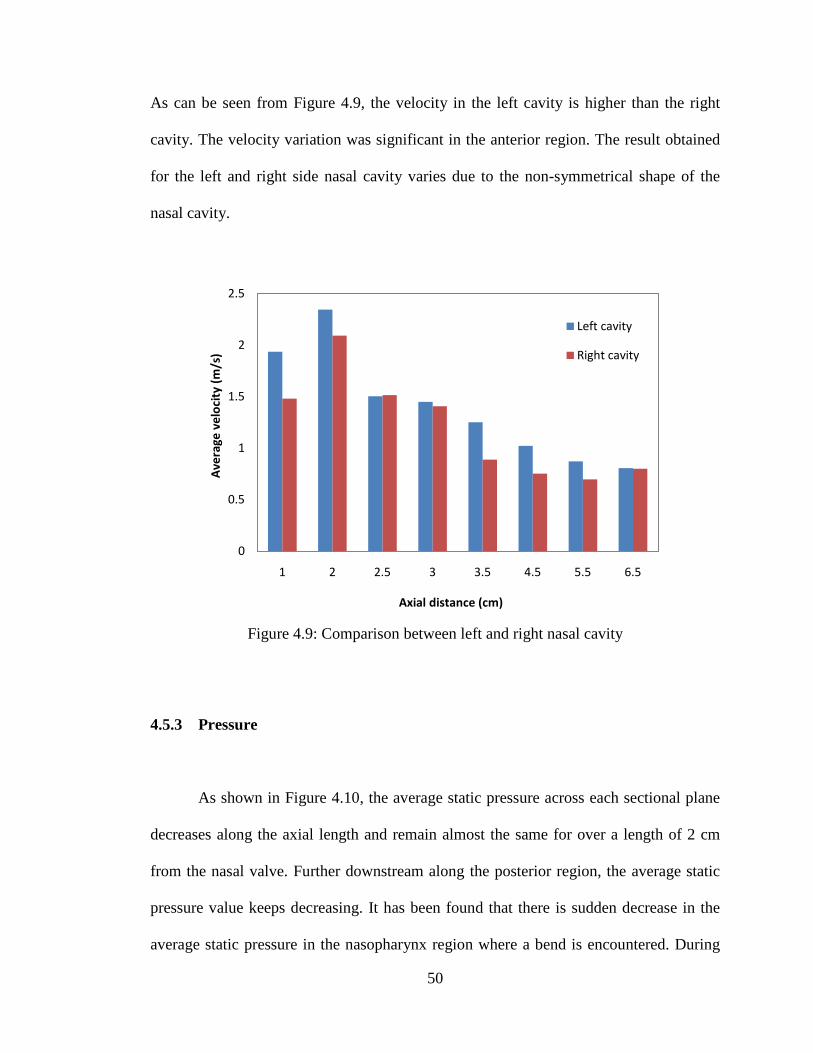
50
As can be seen from Figure 4.9, the velocity in the left cavity is higher than the right
cavity. The velocity variation was significant in the anterior region. The result obtained
for the left and right side nasal cavity varies due to the non-symmetrical shape of the
nasal cavity.
Figure 4.9: Comparison between left and right nasal cavity
4.5.3 Pressure
As shown in Figure 4.10, the average static pressure across each sectional plane
decreases along the axial length and remain almost the same for over a length of 2 cm
from the nasal valve. Further downstream along the posterior region, the average static
pressure value keeps decreasing. It has been found that there is sudden decrease in the
average static pressure in the nasopharynx region where a bend is encountered. During
0
0.5
1
1.5
2
2.5
1 2 2.5 3 3.5 4.5 5.5 6.5
Ave
rage
vel
ocit
y (m
/s)
Axial distance (cm)
Left cavity
Right cavity

51
inspiration, the lungs suck in air from the ambient atmosphere. Hence negative pressure
profile is observed for the inspiratory flow.
Figure 4.10: Average static pressure along the nasal cavity during inspiration
4.5.4 Wall Shear Stress
Figure 4.11 shows the maximum wall shear stress across various sections along
the axial length of the nasal cavity. As seen in Figure 4.11 and Figure 4.12, the highest
wall shear stress can be observed at the anterior and the posterior ends. This may be
attributed to the sudden change in cross section area at the inlet and outlet. The
maximum wall shear stress obtained at the nasal vestibule and nasal valve region is
1.044 Pa and 0.9452 Pa accordingly. The wall shear stress value decrease significantly
after the nasal valve region where the velocity decreases. The wall shear stress value can
be expressed as
-14
-12
-10
-8
-6
-4
-2
0
2
4
6
0 2 4 6 8
Stat
ic P
ress
ure
(Pa)
Axial Distance (cm)
Inspiration
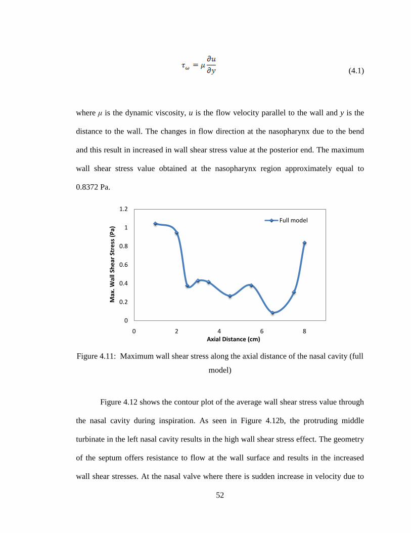
52
(4.1)
where μ is the dynamic viscosity, u is the flow velocity parallel to the wall and y is the
distance to the wall. The changes in flow direction at the nasopharynx due to the bend
and this result in increased in wall shear stress value at the posterior end. The maximum
wall shear stress value obtained at the nasopharynx region approximately equal to
0.8372 Pa.
Figure 4.11: Maximum wall shear stress along the axial distance of the nasal cavity (full
model)
Figure 4.12 shows the contour plot of the average wall shear stress value through
the nasal cavity during inspiration. As seen in Figure 4.12b, the protruding middle
turbinate in the left nasal cavity results in the high wall shear stress effect. The geometry
of the septum offers resistance to flow at the wall surface and results in the increased
wall shear stresses. At the nasal valve where there is sudden increase in velocity due to
0
0.2
0.4
0.6
0.8
1
1.2
0 2 4 6 8
Max
. Wal
l She
ar S
tres
s (P
a)
Axial Distance (cm)
Full model
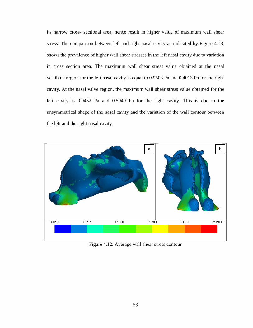
53
its narrow cross- sectional area, hence result in higher value of maximum wall shear
stress. The comparison between left and right nasal cavity as indicated by Figure 4.13,
shows the prevalence of higher wall shear stresses in the left nasal cavity due to variation
in cross section area. The maximum wall shear stress value obtained at the nasal
vestibule region for the left nasal cavity is equal to 0.9503 Pa and 0.4013 Pa for the right
cavity. At the nasal valve region, the maximum wall shear stress value obtained for the
left cavity is 0.9452 Pa and 0.5949 Pa for the right cavity. This is due to the
unsymmetrical shape of the nasal cavity and the variation of the wall contour between
the left and the right nasal cavity.
Figure 4.12: Average wall shear stress contour
a b

54
Figure 4.13: Maximum wall shear stress across left and right nasal cavity
4.5.5 Inspiration vs expiration
In this section, the comparative study of the inspiratory and expiratory states
have been extensively carried out demonstrating the usefulness of numerical models in
better understanding of flow phenomenon inside the nasal cavity and as such should be
of benefit to the medical practitioners.
4.5.5.1 Velocity and pressure comparisons
The flow current that enters the nostril during inspiration progresses towards the
nasal vestibule with a velocity of around 1.8 m/s. Figure 4.14 shows the variation of
velocity along the length of the nasal cavity. The velocity is observed to be higher at the
posterior region during expiration when compared with inspiration. Pressure distribution
as shown in Figure 4.15 showed marked variations while inspiration and expiration. The
0
0.2
0.4
0.6
0.8
1
1.2
1 2 2.5 3 3.5 4.5 5.5 6.5
Max
. Wal
l She
ar S
tres
s (P
a)
Axial Distance (cm)
Left Cavity
Right Cavity

55
Expiratory mechanism is defined by positive pressure gradients. The flow is thrown out
from the lungs and therefore there is prevalence of higher values of pressure during
expiration. Whereas inspiration is the mechanism in which the lungs suck the air from
the ambient atmosphere. Hence negative pressure profile is observed for the inspiratory
flow.
Figure 4.14: Velocity profile comparison during inspiration and expiration
0
0.5
1
1.5
2
2.5
3
3.5
1 2 3 4 5 6 7 8 9 10
Ave
rage
vel
ocit
y (m
/s)
Axial distance (Pa)
InspirationExpirationLeft inspirationRight inspiration

56
Figure 4.15: Average static pressure along the axial length of the nasal cavity
4.5.5.2 Resistance
Different resistance plots are obtained for inspiration and expiration, indicating
the variation of resistance in both processes (see Figure 4.16). Lower resistance values
are obtained on expiration when compared to inspiration. There is ambiguity with
respect to observations on resistance during inspiration and expiration. Haight and Cole,
(1983) noted that during quiet respiration the resistance to airflow was higher during
inspiration when compared with expiration. However Kenyon, (1987) observed the
opposite and found the expiratory resistance to be higher than the inspiratory one. Viani
et al., (1990) found the expiratory resistance to be higher when measured at a pressure
gradient of 150 Pa.
-14
-12
-10
-8
-6
-4
-2
0
2
4
6
0 2 4 6 8 10A
vera
ge s
tati
c pr
essu
re (P
a)
Axial distance (cm)
Inspiration
Expiration
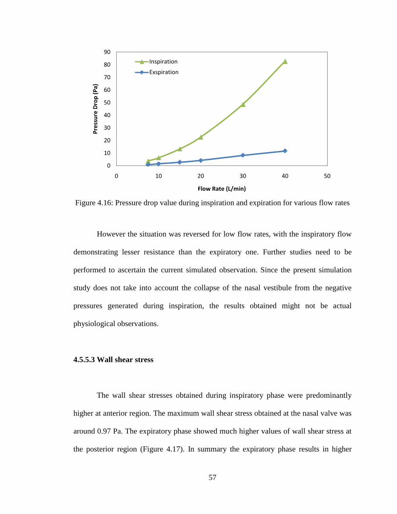
57
Figure 4.16: Pressure drop value during inspiration and expiration for various flow rates
However the situation was reversed for low flow rates, with the inspiratory flow
demonstrating lesser resistance than the expiratory one. Further studies need to be
performed to ascertain the current simulated observation. Since the present simulation
study does not take into account the collapse of the nasal vestibule from the negative
pressures generated during inspiration, the results obtained might not be actual
physiological observations.
4.5.5.3 Wall shear stress
The wall shear stresses obtained during inspiratory phase were predominantly
higher at anterior region. The maximum wall shear stress obtained at the nasal valve was
around 0.97 Pa. The expiratory phase showed much higher values of wall shear stress at
the posterior region (Figure 4.17). In summary the expiratory phase results in higher
0
10
20
30
40
50
60
70
80
90
0 10 20 30 40 50
Pres
sure
Dro
p (P
a)
Flow Rate (L/min)
Inspiration
Exspiration
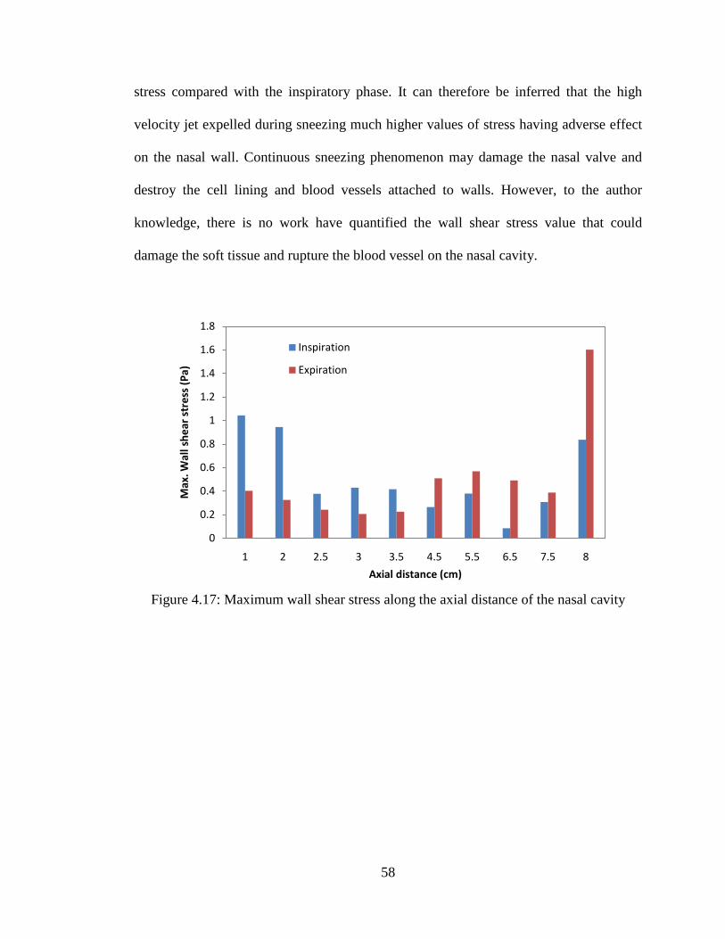
58
stress compared with the inspiratory phase. It can therefore be inferred that the high
velocity jet expelled during sneezing much higher values of stress having adverse effect
on the nasal wall. Continuous sneezing phenomenon may damage the nasal valve and
destroy the cell lining and blood vessels attached to walls. However, to the author
knowledge, there is no work have quantified the wall shear stress value that could
damage the soft tissue and rupture the blood vessel on the nasal cavity.
Figure 4.17: Maximum wall shear stress along the axial distance of the nasal cavity
0
0.2
0.4
0.6
0.8
1
1.2
1.4
1.6
1.8
1 2 2.5 3 3.5 4.5 5.5 6.5 7.5 8
Max
. Wal
l she
ar s
tres
s (P
a)
Axial distance (cm)
Inspiration
Expiration

59
4.6 Various breathing rates for inspiration and expiration
Humans exhibit different breathing rate under different conditions. While
sleeping humans tend to have low breathing flow rates then while working or being
awake. The normal breathing approaches 20 L/min. Under heavy exercise or while
running, the flow rate may increase beyond 40 L/min. Therefore it would be useful to
understand the effect of different breathing flow rates on the nasal cavity. In this section,
the flow characteristics inside a female nasal cavity has been evaluated using CFD for
steady state flow consisting of flow rates varying from 7.5 to 40 L/min in both
inspiration and expiration mechanism.
4.6.1 Average velocity
The average velocity values have been extracted for both inspiration and
expiration at some important location like the vestibule, nasal valve and the
nasopharynx. Figure 4.18 shows the average velocity values for flow rates from 7.5 to 40
L/min obtained at different sections along the nasal cavity during inspiration. As seen in
Figure 4.18, irrespective of the flow rates, the highest value of average velocity appears
at the nasal valve region during inspiration. Under laminar flow rate ranging from 7.5 to
15 L/min, increment of 7.5 L/min, the average velocity value increased by about 120 %.
However, under turbulent conditions having flow rate ranging from 20 to 40 L/min, for
an increment of 20 L/min, the difference in average velocity was only about115 %. The
maximum velocity at the nasal valve region for the flow rates of 7.5 L/min was 1.54 m/s,
which increased to 8.66 m/s for flow rate of 40 L/min. Higher values of velocity at the
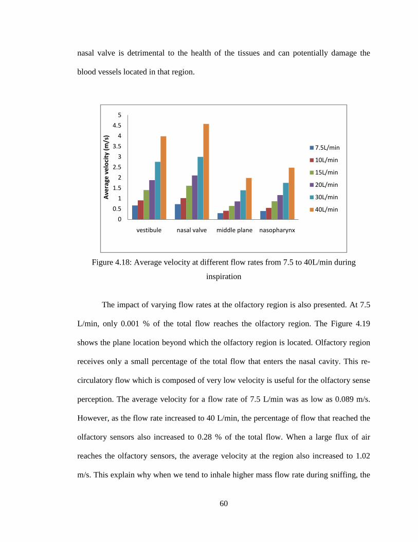
60
nasal valve is detrimental to the health of the tissues and can potentially damage the
blood vessels located in that region.
Figure 4.18: Average velocity at different flow rates from 7.5 to 40L/min during
inspiration
The impact of varying flow rates at the olfactory region is also presented. At 7.5
L/min, only 0.001 % of the total flow reaches the olfactory region. The Figure 4.19
shows the plane location beyond which the olfactory region is located. Olfactory region
receives only a small percentage of the total flow that enters the nasal cavity. This re-
circulatory flow which is composed of very low velocity is useful for the olfactory sense
perception. The average velocity for a flow rate of 7.5 L/min was as low as 0.089 m/s.
However, as the flow rate increased to 40 L/min, the percentage of flow that reached the
olfactory sensors also increased to 0.28 % of the total flow. When a large flux of air
reaches the olfactory sensors, the average velocity at the region also increased to 1.02
m/s. This explain why when we tend to inhale higher mass flow rate during sniffing, the
0
0.5
1
1.5
2
2.5
3
3.5
4
4.5
5
vestibule nasal valve middle plane nasopharynx
Ave
rage
vel
ocit
y (m
/s)
7.5L/min
10L/min
15L/min
20L/min
30L/min
40L/min

61
perception of smell also improves. Studies by Mullins (1955) and Schneider et al.,
(1963) also have shown that an increase in flow rate increases odor detectability.
Figure 4.19: Model of the nasal cavity showing the olfactory plane
However, for expiration, the average velocity value attained at vestibule and
nasal valve region is almost the same as the flow increase from 7.5 to 40 L/min. In
contrast to inspiration, almost uniform velocity profiles can be observed at all locations
under lower flow rates. As shown in Figure 4.20, only marginal variations were
observed between various locations as the flow rate increased.
Olfactory plane
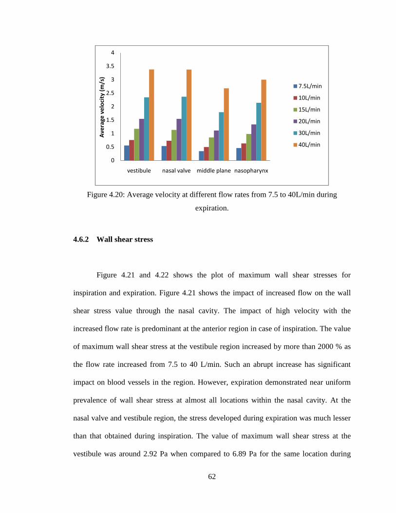
62
Figure 4.20: Average velocity at different flow rates from 7.5 to 40L/min during
expiration.
4.6.2 Wall shear stress
Figure 4.21 and 4.22 shows the plot of maximum wall shear stresses for
inspiration and expiration. Figure 4.21 shows the impact of increased flow on the wall
shear stress value through the nasal cavity. The impact of high velocity with the
increased flow rate is predominant at the anterior region in case of inspiration. The value
of maximum wall shear stress at the vestibule region increased by more than 2000 % as
the flow rate increased from 7.5 to 40 L/min. Such an abrupt increase has significant
impact on blood vessels in the region. However, expiration demonstrated near uniform
prevalence of wall shear stress at almost all locations within the nasal cavity. At the
nasal valve and vestibule region, the stress developed during expiration was much lesser
than that obtained during inspiration. The value of maximum wall shear stress at the
vestibule was around 2.92 Pa when compared to 6.89 Pa for the same location during
0
0.5
1
1.5
2
2.5
3
3.5
4
vestibule nasal valve middle plane nasopharynx
Ave
rage
vel
ocit
y (m
/s)
7.5L/min
10L/min
15L/min
20L/min
30L/min
40L/min

63
inspiration. Therefore the sneezing phenomenon, which is characterized by abrupt and
very high expiratory flow rates of greater than 40 L/min, will produce significantly
lower wall shear stresses than for the same flow rate during inspiration. Hence even
though sneezing is a sudden jet of flow with high velocity, the stresses produced will be
much lesser. However, higher flow rates are not desired, since they result in very high
values of pressure gradients which may result in the collapse of the nasal vestibule as
well induce more stresses in the nasal cavity thereby damaging the delicate tissue layers
and blood vessels creating complications.
Figure 4.21: Maximum wall shear stress values through the axial distance of the nasal
cavity during inspiration
0
1
2
3
4
5
6
7
8
vestibule nasal valve middle plane nasopharynx
Max
. wal
l she
ar s
tres
s (P
a)
7.5L/min
10L/min
15L/min
20L/min
30L/min
40L/min

64
Figure 4.22: Maximum wall shear stress values through the axial distance of the nasal
cavity during expiration
0
0.5
1
1.5
2
2.5
3
3.5
vestibule nasal valve middle plane nasopharynx
Max
. wal
l she
ar s
tres
s (P
a)
7.5L/min
10L/min
15L/min
20L/min
30L/min
40L/min

65
4.7 Preliminary work on gender comparison
Evidence suggests that there is no gender difference in upper airway size whether
measured directly by imaging methods or indirectly by measurement of upper airway
resistance. (Rowley et al, 2001). However some of the problems like obstructive sleep
apnea are specific to only males (Suzina et al., 2003). The anatomical variations
contribute to gender based occurrence of certain anomalies. Hence gender is one of the
contributing factors for the difference in the flow behavior.
4.7.1 Geometry comparison
In order to verify the anatomical differences based on gender, the length of the
nasal cavity was measured from a sample of available CT images. As a result a sample
of 4 cases each of male and female CT nasal images were measured. Table 4.1 shows
the total length of the nasal cavity obtained from the CT scan images of four male and
four female human subjects. It was found that the female models were slightly smaller in
length when compared to the male models. Based on the results shown in Table 4.1, we
can conclude that female have shorter length of nasal cavity when compared to their
male counterparts. However, this is just sample evidence which need to be corroborated
with much higher samples to verify the observations reported in Table 4.1.

66
Table 4.1: The total length of the nasal cavity based on the gender comparison
Name Length (mm) Female 1 85.72 Female 2 89.78 Female 3 88.90 Female 4 90.97 Male 1 96.69 Male 2 91.73 Male 3 98.48 Male 4 97.37
The current work is focussed on computational study of nasal cavity, hence in
order to further the understanding of the effect of gender based anatomical differences
on the flow behaviour; numerical analysis has been carried out. Most of previous works
on numerical studies of nasal cavity based their observation on male models while the
current research is using female models that developed from CT images.
Figure 4.23: The comparison of cross section area through the nasal cavity of the human
male and female subjects
0
1
2
3
4
5
6
7
0 2 4 6 8 10
Cros
s se
ctio
n ar
ea (c
m2 )
Axial distance (cm)
Cheng et al., (1996)Wen et al., (2008)Female model 1Female model 2Female model 3

67
Figure 4.23 shows the cross section area obtained based on the planes created
across the nasal cavity. The female computational models are compared with the
available male nasal cavity models from the previous published works. As seen in Figure
4.23, the total length of the nasal cavity for female subjects is shorter compared to the
male model developed by Cheng et al., 1996 and Wen et al., 2008. The location of the
nasal valve region also varied for each nasal model. Irrespective of gender this
difference in location has also been reported in previous literature (Keyhani et al., 1995,
Subramanium et al., 1998, Cheng et al., 1996). It also can be observed that the cross
section area at the turbinate region for the female nasal cavity is wider compared to
male. As seen in Figure 4.23, at the posterior region of the nasal airway, a substantial
increase in cross section area was observed after the turbinate region for male.
Conversely, the cross section area of the female nasal airway decreased drastically after
the turbinate region. Thus it was observed that the female possessed smaller cross
section area at nasopharynx. The cross section area at the nasopharynx is 5.8 cm2 and
5.25 cm2 for male and 2.85 cm2, 3.52 cm2 and 2.96 cm2
The nasal resistance in the case of female model also follows the same pattern as
that of the male subject for laminar flow conditions. However under turbulent
conditions, resistance curves as seen in Figure 4.24 is steeper. There are significant
differences in the values of pressure drop obtained for all the 3 female models. Model 1
exhibited higher values of resistance compared to the male model. The value of
resistance for female case 2 was much lesser than that of the male model and the female
case 1. Also the female case 3 showed lower values of resistance than its male
counterparts.
for female nasal cavity. Thus the
female nasal cavity is shorter in length and has smaller posterior cross sectional area.
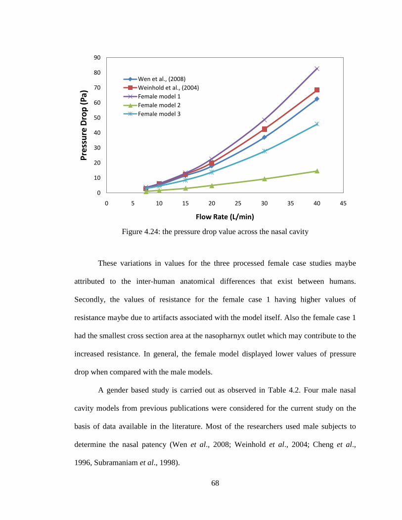
68
Figure 4.24: the pressure drop value across the nasal cavity
These variations in values for the three processed female case studies maybe
attributed to the inter-human anatomical differences that exist between humans.
Secondly, the values of resistance for the female case 1 having higher values of
resistance maybe due to artifacts associated with the model itself. Also the female case 1
had the smallest cross section area at the nasopharnyx outlet which may contribute to the
increased resistance. In general, the female model displayed lower values of pressure
drop when compared with the male models.
A gender based study is carried out as observed in Table 4.2. Four male nasal
cavity models from previous publications were considered for the current study on the
basis of data available in the literature. Most of the researchers used male subjects to
determine the nasal patency (Wen et al., 2008; Weinhold et al., 2004; Cheng et al.,
1996, Subramaniam et al., 1998).
0
10
20
30
40
50
60
70
80
90
0 5 10 15 20 25 30 35 40 45
Pres
sure
Dro
p (P
a)
Flow Rate (L/min)
Wen et al., (2008)Weinhold et al., (2004)Female model 1Female model 2Female model 3

69
Table 4.2: Characteristic description of nasal cavity for male and female nasal cavity
models
Particulars Male Female
Total length of the nasal cavity
9.2 cm (Wen et al., 2008) 9.3 cm (Cheng et al., 1996)
8.5 cm (Model 1) 8.0 cm (Model 2) 9.0 cm (Model 3)
Nasapharynx cross sectional area
5.25 cm2 (Wen et al., 2008) 5.8 cm2 (Cheng et al., 1996)
2.85 cm2 (Model 1) 3.52 cm2 (Model 2) 2.96 cm2 (Model 3)
The location of the nasal valve region
3.3 cm (Cheng et al., 1996) 2.0 cm (Wen et al., 2008)
2.0 cm (Model 1) 1.65 cm (Model 2) 2.0 cm (Model 3)
Nasal valve cross section area
1.4 cm2 (Wen et al., 2008) 1.8 cm2 (Cheng et al., 1996)
1.5 cm2 (Model 1) 1.26 cm2 (Model 2) 1.84 cm2 (Model 3)
Pressure drop (for flow rate of 20L/min)
18 Pa (Wen et al., 2008) 20 Pa (Weinhold et al., 2004)
22.6 Pa (Model 1) 4.88 Pa (Model 2) 13.88Pa (Model 3)
Maximum velocity at nasal valve (for flow rate of 15L/min)
4.2 m/s (Subramaniam et al., 1998)
3.17 m/s (Model 1) 2.68 m/s (Model 2) 2.23 m/s (Model 3)
As seen in Table 4.2, the female model has shorter length of nasal cavity (8.5 cm,
8 cm and 9 cm) when compared with that of the male subjects as determined by Cheng
et al., (1996) and Wen et al., (2008) to be 9.3 cm and 9.2 cm respectively. Also another
important observation was the decrease in the cross-sectional area of the female subject
when compare to male in the posterior region. The nasopharynx cross section area

70
obtained for this study was 2.85 cm2, 3.52 cm2 and 2.96 cm2; while 5.25 cm2 and 5.8 cm2
Although we do find anatomical variation between male and the female model, a
general trend can be observed. An increase in the cross-sectional profiles was observed
after the nasal valve region. For the present geometry, the nasal valve region was located
about 2.0 cm, 1.65 cm and 2 cm from the anterior tip of nose, which compares with the
other models that were located at 3.3 cm and 2.0 cm as obtained by Cheng et al., (1996)
and Wen et al., (2008) respectively. As stated earlier, irrespective of gender, the
difference in location has also been reported in previous literature (Keyhani et al., 1995,
Subramanium et al., 1995, Cheng et al., 1996).
was determined by Wen et al., (2008) and Cheng et al., (1996) respectively. This clearly
indicated that the male nasal cavity had larger posterior cross sectional area, emphasising
the variation based on gender.
One of the advantages of using CFD is its accurate presentation of the
physiological function associated with the nasal cavity. It presents useful quantification
between the male and the female physiological function. The pressure drop at 20 L/min
obtained for the female nasal cavities was 22.6 Pa for model 1, 4.8 Pa for model 2, and
13.88 Pa for model 3 when compared with male model at around 18 Pa & 20 Pa for the
same flow rate obtained by Wen et al., (2008) and Weinhold et al., (2004)
Nasal valve being the critical area of the nasal cavity, comparison between the
male and female models resulted in the female models exhibiting lesser value of
respectively.
The female model 1 had the smallest cross section area at the nasopharnyx outlet hence
the higher value of pressure drop was obtained in comparison to model 2 and model 3.
However, in general the value of pressure drop for female case 2 and 3 is lower than the
male models reported in the literature.

71
maximum velocity when compared with the male model developed by Subramanian et
al., 1998 the value of maximum velocity obtained for the three female models are 3.17
m/s, 2.68 m/s, and 2.23 m/s respectively as against 4.2m/s for similar flow rate obtained
for the male model. This shows the relative difference between the male and the female
flow behaviour.
The current study has identified certain gender based anatomical and
physiological differences. The use of computational fluid dynamic has assisted in the
understanding of these differences which could not be earlier quantified based on mere
medical observation and devices. Also, it has highlighted the fact that numerical models
cannot be generalized for quantification because gender based differences exists. Hence
in all the future numerical study of flow through the nasal cavity, it is imperative to
mention the gender of the model under consideration.

72
4.8 Gravity effect on nasal airflow due to the change of posture
The influence of postural changes in nasal cavity has been investigated in this
section. Many reasons have been cited for the increase in the nasal resistance, from
increase in the central venous pressure resulting in congestion of the nasal mucosa, also
pressing of some of the body areas result in the change in nasal resistance (Roithmann et
al., 2005). Hence the posture change is an important determinant of upper airway
dimensions. The aggravating effect of the supine body position on breathing
abnormalities during sleep is attributed to the effect of gravity on the upper airway
(Oksenberg and Silverberg, 1998).
Several medical literatures cite the changes in variation in the pharyngeal area
with change in posture. But due to the difficulty involved in obtaining CT scan of the
person in sitting posture, the CT data obtained in the supine position is utilized to study
the effect of posture on the flow. Therefore, this study assumes no changes in the
dimension of the nasal cavity with the change in posture. However, the change in the
direction of the gravity force acts based on the change of posture is considered for this
study. Four cases namely sitting, supine, prone and recumbence right are considered.
The acceleration due to gravity is taken to be 9.81 m/s2
at sea level. The body force
weighted pressure discretization scheme is adopted in the numerical simulation where
the discontinuity of explicit body forces (e.g. gravity, swirl) was taking into account.

73
Figure 4.25: Variation of Average static pressure with posture
Figure 4.26: Effect of change of posture on velocity at 15L/min
-0.3
-0.25
-0.2
-0.15
-0.1
-0.05
4E-16
0.05
0.1
0.15
0.2
0.25
0.3
0.35
2.5 3.5 4.5 5.5 6.5Pres
sure
(Pa)
Axial Distance (cm)
SITTING
SUPINE
RIGHT RECUMBENCY
1.4
1.45
1.5
1.55
1.6
1.65
1.7
1.75
1.8
1.85
3.5 4.5 5.5 6.5 7.5
Max
. Vel
ocit
y(m
/s)
Axial Distance(cm)
SITTING
SUPINE
PRONE

74
As seen from the Figure 4.25, around 0.3 % change in the average static pressure
is observed while changing from sitting to supine position. Along the middle region the
average static pressure decreases as we change position from sitting to supine. Also
significant changes were observed on shifting to right recumbency position. These
results show the influence of gravity associated with the change in posture.
Figure 4.26 shows the variation in the maximum velocity beyond the nasal valve
region (3.5 cm to 7.5 cm). Significant drop in velocity can be seen while shifting from
sitting to supine position. Not much variation in velocity was observed between the
supine and the prone position.
Figure 4.27: Variation in maximum wall shear stresses with change of posture
Also the change in posture had significant effect on the wall shear stresses as can
be observed from Figure 4.27. The contours shown in Figure 4.28, shows the effect of
change of posture on the flow separation. We can observe that the flow along the right
0.245
0.25
0.255
0.26
0.265
0.27
0.275
0.28
0.285
2.5 3 3.5 5.5
wal
l she
ar s
tres
s (P
a)
Axial Distance (cm)
SITTING
SUPINE
RIGHT RECUMBENCYPRONE
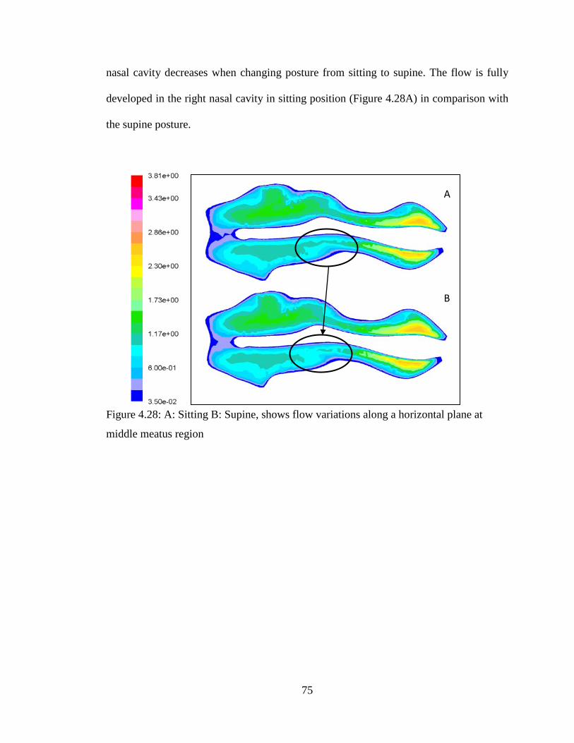
75
nasal cavity decreases when changing posture from sitting to supine. The flow is fully
developed in the right nasal cavity in sitting position (Figure 4.28A) in comparison with
the supine posture.
Figure 4.28: A: Sitting B: Supine, shows flow variations along a horizontal plane at
middle meatus region
A
B

76
4.9 Effect of different boundary condition on flow parameters
The authors investigate the effect of various boundary conditions classified as
plug flow for boundary values defined at nostril inlet and pull flow which simulates the
natural physiological breathing conditions with boundary defined at nasopharynx.
Figure 4.29: Plug flow boundary condition for inspiration A and expiration B
Figure 4.30: Pull flow boundary condition for inspiration A and expiration B.
Inspiratory steady airflow numerical simulations were carried out using 3D nasal cavity
model derived from tomography scan images. Figures 4.29 and 4.30 show the plug and
pull flow boundary condition definition for inspiration and expiration. Plug and pull flow
boundary conditions were employed on the same model and compared to evaluate the
effect of different boundary conditions on the flow parameters. Studies are carried out
Mass flow inlet Outflow
Pressure inlet Pressure outlet
Mass flow inlet Pressure outlet
Pressure outlet Pressure inlet
A
A
B
B

77
for various flow rates of 7.5 L/min, 10 L/min, 15 L/min, 20 L/min, 30 L/min and 40
L/min suggesting various breathing rates.
4.9.1 Nasal Resistance comparison for plug-flow and pull-flow
Numerical methods are subjected to various assumptions especially with respect
to boundary definition. In order to acquire a more realistic value of nasal resistance,
comparative study is performed to understand the effect of boundary condition on the
values of resistance determined. Figure 4.31 gives the plot of pressure drop across nasal
airway for different flow rates. The pressure drop value increases as the flow rate
increases in both cases. The plug flow condition produced substantially high value of
pressure drop when compared to pull flow boundary condition. Beyond 20 L/min the
pressure drop value increased more drastically for plug flow.
Figure 4.31: Nasal Resistance for different airflow rate
0
10
20
30
40
50
60
70
80
90
0 10 20 30 40 50
Pres
sure
dro
p (P
a)
Flow rates (L/min)
Plug flow
Pull flow

78
It can be observed that the differences between plug flow and pull flow for
inspiration is quite large as observed in Figure 4.32. At the nasal valve, the resistance for
plug flow was 0.311 Pa-min/L and for pull flow the value was 0.147 Pa-min/L.
Maximum variation was noticed at the vestibule region with 0.3578 Pa-min/L.
In case of the plug flow, the air is forced through the nostrils into the nasal
cavity. This explains the prevalence of higher values of pressure drop and nasal
resistance in case of the plug flow boundary condition. Hence, it is clear from the
pressure drop and the resistance plots that different boundary condition result in
variation in flow properties. Therefore, it is very important to adopt the most appropriate
boundary condition to evaluate the nasal physiology.
Figure 4.32: Inspiratory nasal resistance for 15 L/min at vestibule, nasal valve, middle
section and nasopharynx.
0.0
0.1
0.2
0.3
0.4
0.5
0.6
1 2 4.5 7.5
Nas
al r
esis
tanc
e (P
a/L/
min
)
Axial distance (cm)
Pull flow
Plug flow

79
4.9.2 Velocity
Figure 4.33 shows the effect of different boundary condition on velocity along
the length of the nasal cavity. Since it was found that similar pattern for all flow rates
investigated, the result of only 15 L/min simulation is presented. The average velocity
values varied along the axial length of the nasal passage. This can be attributed to the
change of cross section area along the nasal passage. Plug-flow model and pull-flow
case study exhibited differences in the velocity profile. The nasal vestibule and the
narrow constrict called the nasal valve showed major variations with respect to velocity
profile between plug and pull flow boundary.
Figure 4.33: Velocity plot along the axial distance (at 15 L/min).
The average velocity for nasal vestibule and nasal valve is 1.4 m/s and 1.6 m/s
for plug flow. Whereas, for pull flow case, the average velocity value in nasal vestibule
and nasal valve region was observed to be around 0.96 m/s and 1.41 m/s respectively.
0
0.2
0.4
0.6
0.8
1
1.2
1.4
1.6
1.8
1 2 4.5 7.5
Avg
. Vel
ocit
y (m
/s)
Axial distance (cm)
Inspiration- Plug flow
Inspiration-Pull flow
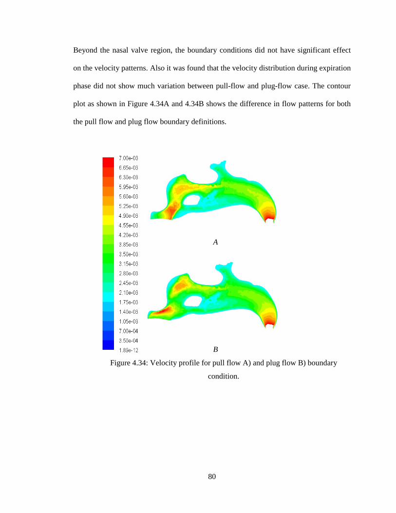
80
Beyond the nasal valve region, the boundary conditions did not have significant effect
on the velocity patterns. Also it was found that the velocity distribution during expiration
phase did not show much variation between pull-flow and plug-flow case. The contour
plot as shown in Figure 4.34A and 4.34B shows the difference in flow patterns for both
the pull flow and plug flow boundary definitions.
A
B
Figure 4.34: Velocity profile for pull flow A) and plug flow B) boundary
condition.
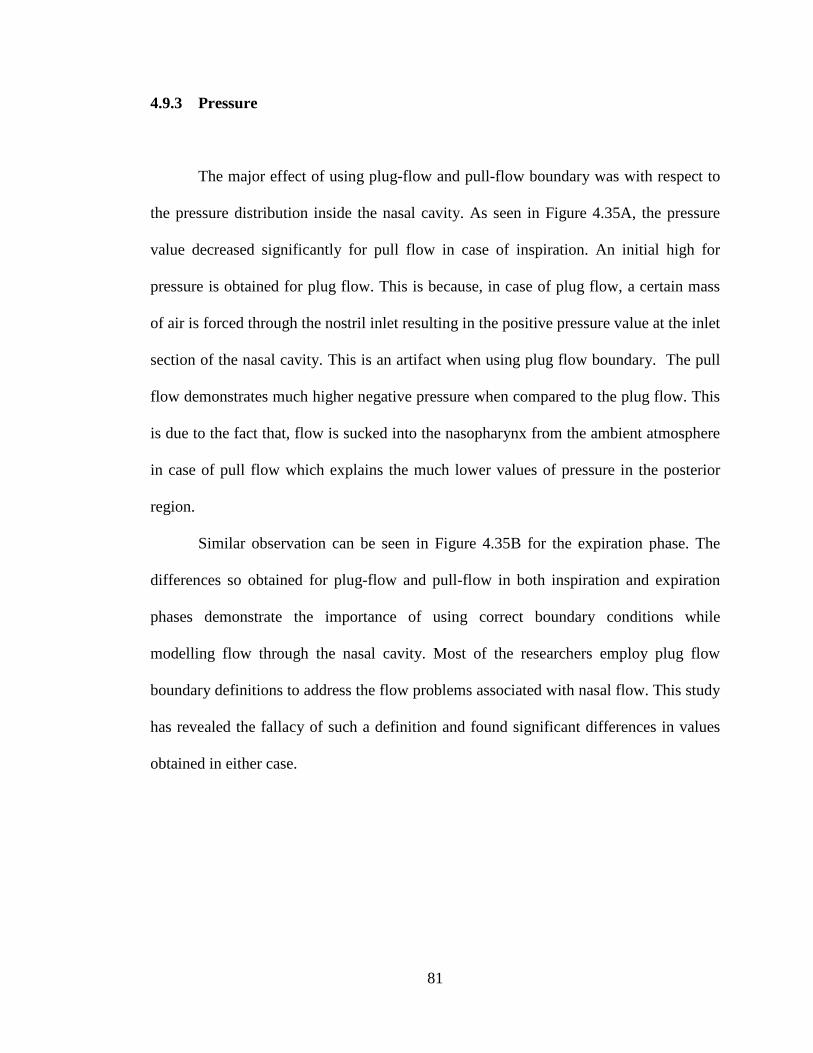
81
4.9.3 Pressure
The major effect of using plug-flow and pull-flow boundary was with respect to
the pressure distribution inside the nasal cavity. As seen in Figure 4.35A, the pressure
value decreased significantly for pull flow in case of inspiration. An initial high for
pressure is obtained for plug flow. This is because, in case of plug flow, a certain mass
of air is forced through the nostril inlet resulting in the positive pressure value at the inlet
section of the nasal cavity. This is an artifact when using plug flow boundary. The pull
flow demonstrates much higher negative pressure when compared to the plug flow. This
is due to the fact that, flow is sucked into the nasopharynx from the ambient atmosphere
in case of pull flow which explains the much lower values of pressure in the posterior
region.
Similar observation can be seen in Figure 4.35B for the expiration phase. The
differences so obtained for plug-flow and pull-flow in both inspiration and expiration
phases demonstrate the importance of using correct boundary conditions while
modelling flow through the nasal cavity. Most of the researchers employ plug flow
boundary definitions to address the flow problems associated with nasal flow. This study
has revealed the fallacy of such a definition and found significant differences in values
obtained in either case.
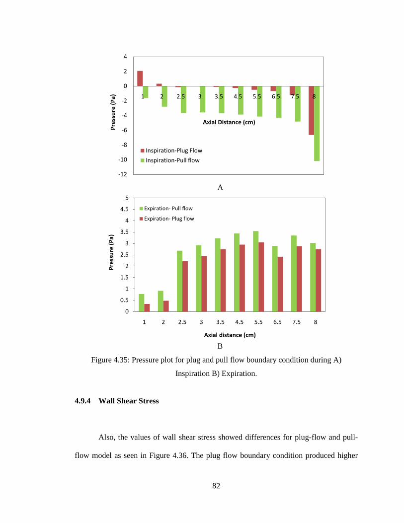
82
A
B
Figure 4.35: Pressure plot for plug and pull flow boundary condition during A)
Inspiration B) Expiration.
4.9.4 Wall Shear Stress
Also, the values of wall shear stress showed differences for plug-flow and pull-
flow model as seen in Figure 4.36. The plug flow boundary condition produced higher
-12
-10
-8
-6
-4
-2
0
2
4
1 2 2.5 3 3.5 4.5 5.5 6.5 7.5 8
Pres
sure
(Pa)
Axial Distance (cm)
Inspiration-Plug Flow
Inspiration-Pull flow
0
0.5
1
1.5
2
2.5
3
3.5
4
4.5
5
1 2 2.5 3 3.5 4.5 5.5 6.5 7.5 8
Pres
sure
(Pa)
Axial distance (cm)
Expiration- Pull flow
Expiration- Plug flow
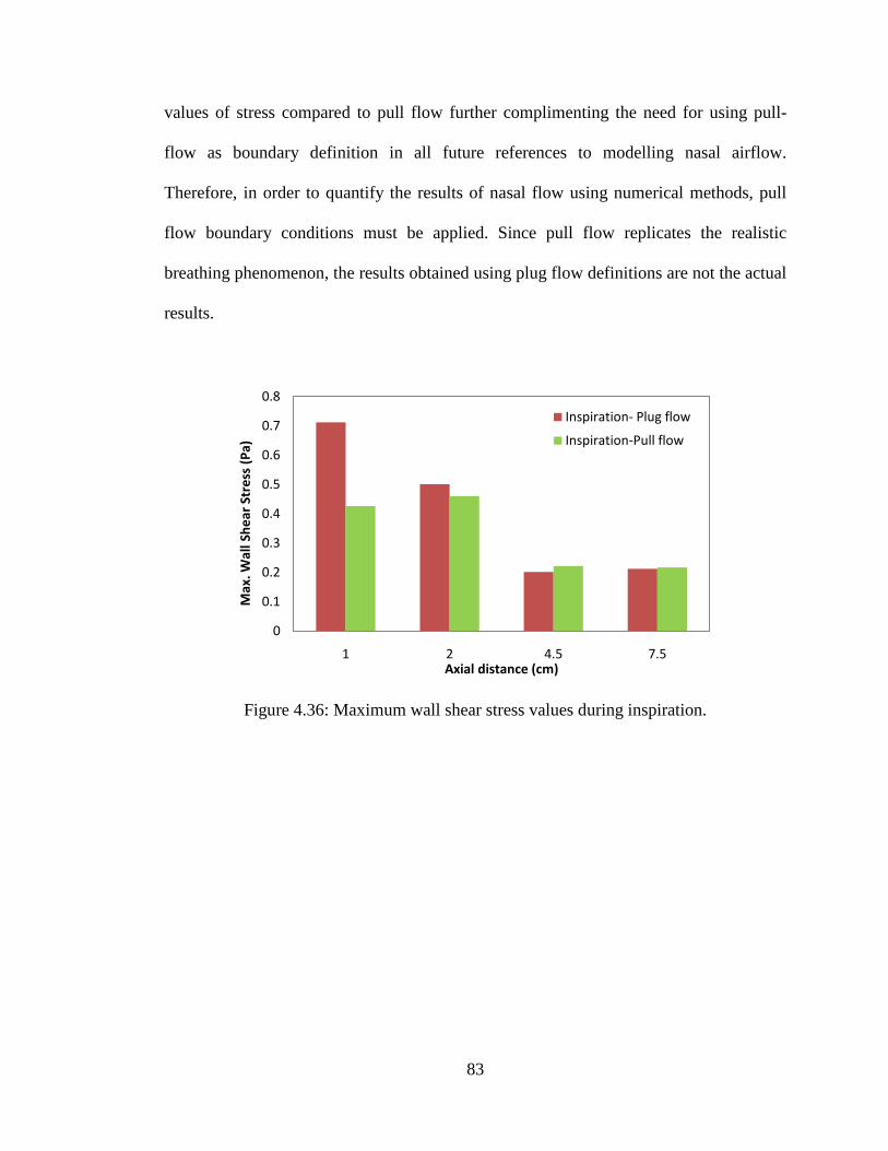
83
values of stress compared to pull flow further complimenting the need for using pull-
flow as boundary definition in all future references to modelling nasal airflow.
Therefore, in order to quantify the results of nasal flow using numerical methods, pull
flow boundary conditions must be applied. Since pull flow replicates the realistic
breathing phenomenon, the results obtained using plug flow definitions are not the actual
results.
Figure 4.36: Maximum wall shear stress values during inspiration.
0
0.1
0.2
0.3
0.4
0.5
0.6
0.7
0.8
1 2 4.5 7.5
Max
. Wal
l She
ar S
tres
s (P
a)
Axial distance (cm)
Inspiration- Plug flow
Inspiration-Pull flow

84
CHAPTER 5
CONCLUSION
5.1 Introduction
Three dimensional computational model of female human nasal cavity were developed
based on the CT scans of Malaysian female subjects. Numerical simulation of
inspiratory and expiratory airflow was performed for flow rates of 7.5, 10, 15, 20, 30,
and 40 L/min using the developed models. This work on nasal flow study utilized female
nasal cavity models as against the male models used by previous researchers. Numerical
study carried on the female models has been validated with that of the male models from
the data available in the literature as described in section 4.4. The effect of gender based
anatomical differences on the flow behaviour also has been investigated. The effect of
gravity due to change of posture is also studied. Plug flow and pull flow boundary
conditions are evaluated and its effect on the nasal flow are also analyzed. In this
chapter, major results, limitations of present work, and recommendation for future study
are discussed.
5.2 Major conclusions drawn from this study
The following conclusions are presented based on each study topic.

85
5.2.1 Basic airflow studies
The flow was observed to be fully developed along the middle meatus region
while the superior and inferior meatus pathway received lesser flow. This finding was
consistent with that of the previous researchers (Hahn et al., 1993; Segal et al., 2008).
There was sudden increase of average velocity value at the nasopharynx region which
could be attributed to the decrease in cross section area at the posterior region of the
nasal geometry. The nasal valve which is located at a distance of around 2 cm from the
anterior region of the nasal cavity, attained the maximum velocity at around 4.18 m/s as
against 4.82 m/s & 3.1 m/s obtained by Xiong et al., (2008) and Croce et al., (2006)
respectively. The peak airspeed in each plane decreases posteriorly beyond nasal valve
region as the cross sectional area increase. The average static pressure value decreases
posteriorly along the nasal cavity. At the nasal valve where there is sudden increase in
velocity due to its narrow cross- sectional area, resulted in the prevalence of higher wall
shear stresses. The geometry of the septum also offered resistance to flow at the wall
surface and results in the increased wall shear stresses. The flow changes direction at the
nasopharynx due to the bend and this resulted in increase in wall shear stress at the
posterior end. The low velocity re-circulating stream was found just posterior to the
nasal valve region. This low velocity recirculatory flow at the olfactory region stimulates
the olfactory nerves which is responsible for our sense of smell.
It can therefore be concluded that, the complicated anatomy of the nasal cavity
has been designed to attain the physiological function desired for normal breathing. It is
this structure that makes possible the sense of smell and conditioning of inspired air.
86
5.2.2 Various breathing rates for inspiration and expiration
Humans exhibit different breathing rate under different conditions. Irrespective
of the flow rates, the highest value of average velocity appears at the nasal valve region
during inspiration. Olfactory region received only a small percentage of the total flow
that entered the nasal cavity. The perception of smell was improved with increased flow
rates. The value of maximum wall shear stress at the vestibule region increased by more
than 2000 % as the flow rate increased from 7.5 to 40 L/min. Such an abrupt increase
has significant impact on blood vessels in the region. The value of maximum wall shear
stress at the vestibule was around 2.92 Pa when compared to 6.89 Pa for the same
location during inspiration. Therefore the sneezing phenomenon, which is characterized
by abrupt and very high expiratory flow rates of greater than 40 L/min, will produce
significantly lower wall shear stresses than for the same flow rate during inspiration.
Hence even though sneezing is a sudden jet of flow with high velocity, the stresses
produced will be much lesser. However, higher flow rates are not desired, since they
result in very high values of pressure gradients which may result in the collapse of the
nasal vestibule as well induce more stresses in the nasal cavity thereby damaging the
delicate tissue layers and blood vessels creating complications.
5.2.3 Gravity effect on nasal airflow due to the change of posture
From the literature review it was established that the change of posture
significantly affects the breathing patterns (Beaumont et al., 1998; Hsing-won Wang,
2002; Matsuzawa et al., 1995; Tvinnereim et al., 1996). Hence the gravity effect due to
87
the change of posture significantly influences the flow parameters and cannot be
neglected. These findings hold significant importance in the study of numerical analysis
of flow through the nasal cavity. The 3D model for developing the nasal cavity is
obtained either from the MRI or the CT scans. Hence the numerical modelling
associated with posture dynamics comes into effect. Therefore while applying the
boundary conditions in the study of nasal flow using CFD; we must take into account the
effect of posture and gravity. As per our knowledge none of the previous studies on
numerical flow analysis take into account the effect of posture and gravity. Therefore in
order to accurately predict the flow features inside the nasal airway path, we must
specify the correct posture and apply appropriate boundary conditions. This study on
effect of gender and posture can be considered as the major step towards standardisation
of modelling approach in the domain of nasal flow studies.
5.2.4 Effect of different boundary condition on flow parameters
A 3D computational study of inspiratory airflow using plug and pull flow boundary
conditions was carried out. Comparative analysis of plug flow and pull flow boundary
conditions showed significant variations for various flow parameters like velocity and
pressure distribution. Velocity at the vestibule and the nasal valve region was higher for
plug flow when compared with pull flow. There was a very significant difference in the
pressure distribution across the nasal cavity. Considerable variation was observed for
resistance across the nasal cavity for pull flow and plug flow cases. The flow patterns
obtained during either case were different. Hence, in order to account for the natural
physiological breathing conditions, it is very important to include the correct boundary
88
condition. Since pull flow accounts for the natural physiological boundary definition,
future research should incorporate pull-flow boundary in order to study the physiology
of the nasal cavity. Based on the study, it can be concluded that difference in boundary
condition will result in variation in flow behavior inside the nasal cavity. In the absence
of standardization of modelling of flow through the nasal cavity, and lack of unanimity
among the researchers on the type of boundary conditions to be applied, this study holds
significant importance.
5.3 Future works
Based on the presented research findings, several recommendations can be drawn
to facilitate and provide future direction of research works. First, higher quality of CT
scan images with better pixel resolution and smaller number of increment between slice
of image are need to capture accurately the nasal cavity. Highly quality of CT scan
images will help reduce the time required to build the complex geometry of the nasal
cavity and avoid the creation of ‘stair-step’ surface contour which will affect the airflow
characteristic.
In order to capture the exact physiological nasal breathing, modelling the
collapsibility of the nasal vestibule region during inspiration can be considered as a vital
step. However, the inclusion of this work in the current research study which demands
the study of fluid structure interaction is not possible due to the complicated structure of
the nasal cavity and time constraint.
The implication of the study on posture holds importance in the future study of
medicine delivery through the nasal cavity. It would be interesting to understand the

89
relationship in arriving at the appropriate posture for the delivery of medicine and the
effectiveness of this posture for the drugs to reach the desired locations inside the nasal
cavity. The study of gender effect on the nasal airflow in the future research work may
also include the age and body size variation which also can be the contributing factors
that affecting the nasal patency.
Further study may also be carried out to study the posture effect on nasal
breathing by simulating the nasal model which developed based on the CT scan images
obtained according to sitting, supine, prone and right recumbency position. Study of
nasal abnormality can also be performed in order to assist ENT surgeon in pre-diagnosis
of the nasal disease and plan for the treatment planning of nasal surgeries.
90
REFERENCES Ahmad KA, Abdullah MZ, Watterson JK. 2010. Numerical modelling of a pitching airfoil. Jurnal Mekanikal. 30: 37-47. Austin CE, Foreman JC. 1994. Acoustic rhinometry compared with posterior rhinomanometry in the measurement of histamine- and bradykinin-induced changes in nasal airway patency. Br J clin Pharmac. 37: 33-37. Bailie N, Hanna B, Watterson J, Gallagher G. 2006. An overview of numerical modeling of nasal airflow. Rhinology 44(1): 53-57. Beaumont M, Fodil R, Isabey D, Lofaso F, Touchard D, Harf A, Louis B. 1998. Gravity effects on upper airway area and lung volumes during parabolic flight. J Appl Physiol. 84: 1639-1645. Cheng YS, Yeh HC, Guilmette RA, Simpson SQ, Cheng KH, Swift DL. 1996. Nasal deposition of ultrafine particles in human volunteers and its relationship to airway geometry. Aerosol Sci Technol. 25(3): 274-291. Corey JP. 2006. Acoustic rhinometry: should we be using it? Current opinion in otolaryngology & head and neck surgery. 14(1): 29-34. Croce C, Fodil R, Durand M, Sbirlea-Apiou G, Papon JF, Blondeau JR, Coste A, Isabey D, Louis B. 2006. In vitro experiments and numerical simulations of airflow in realistic nasal airway geometry. Annals of Biomedical Engineering, 34(6): 997-1007. Devyani L, Corey JP. 2004. Acoustic rhinometry and its uses in rhinology and diagnosis of nasal obstruction. Facial plastic surgery clinics of North America. 12(4): 397-405. Ecckes R. 1998. The relationship between subjective & objective measures of nasal function. Jpn J. Rhinol. 37: 61-69. Elad D, Liebenthal R, Wenig BL, Einav S. 1993. Analysis of airflow patterns in the human nose. Med & Biol Eng & Comput. 31: 585-592. Elad D, Wolf M, Keck T. 2008. Air conditioning in the human nasal cavity. Respiratory Physiology & Neurobiology. 163: 121-127. FLUENT 6.1, User guide Garcia GJM, Bailie N, Martin DA, Kimbell JS. 2007. Atrophic rhinitis: a CFD study of air conditioning in the nasal cavity. J Appl Physiol. 103: 1082-1092.
91
Hahn I, Scherer PW, and Mozell MM. 1993. Velocity Profiles Measured for Airflow Through a Large Scale Model of the Human Nasal Cavity. J Appl Physiol. 75(5): 2273-2287. Haight JSJ, Cole P. 1983. The site and function of the nasal valve. Laryngoscope. 93: 49-55. Hilberg O, Jackson AC, Swift DL, Pedersen OF. 1989. Acoustic rhinometry: evaluation of the nasal cavity by acoustic rhinometry. J Appl Physiol. 66: 295-303. Hsing-won Wang. 2002. Effects of posture on nasal resistance. J Med Sci. 22(4): 161-164. Inthavong K, Wen J, Tian ZF, Tu J. 2007. Numerical study of fibre deposition in a human nasal cavity. Aerosol science. 39: 253-265. Ishikawa S, Nakayama T, Watanabe M, Matsuzawa T. 2009. Flow mechanisms in the human olfactory groove. Arch Otolaryngol Head Neck Surg. 135(2): 156-162. Jones AS and Lancer M. 1987. Rhinomanometry. Clin Otolaryngol. 12: 233-236. Kenyon GS. 1987. Phase variation in nasal airway resistance as assessed by active anterior rhinomanometry. Journal of Laryngology and Otology. 101: 910-916. Keyhani K, Scherer PW, Mozell MM. 1995. Numerical simulation of airflow in the human nasal cavity. J. Biomech. Eng. 117: 429–441. Kjærgaard T, Cvancarova M, Steinsvag SK. 2009. Relation of nasal air flow to nasal cavity dimensions. Arch Otolaryngol Head Neck Surg. 135(6): 565-570. Lindemann J, Brambs HJ , Keck T, Wiesmiller KM, Rettinger G, Pless D. 2005. Numerical simulation of intranasal airflow after radical sinus surgery. American Journal of Otalarynology-Head and Neck Medicine & Surgery. 26: 175-180. Liu Y, Matida EA, Gu J, Johnson MR. 2007. Numerical simulation in a 3-D human nasal cavity using RANS, RANS/EIM, and LES. Aerosol Sciences. 38: 683-700. Mamikoglu B, Houser S, Akbar I, Ng B, Corey J P. 2000. Acoustic rhinometry and computed tomography scans for the diagnosis of nasal septal deviation, with clinical correlation. Otolaryngology--head and neck surgery : official journal of American Academy of Otolaryngology-Head and Neck Surgery 123(1 Pt 1): 61-8. Martin SE, Mathur R, Marshall I, Douglas NJ. 1997. The effect of age, sex, obesity and posture on upper airway size. Eur Respir J. 10: 2087-2090.
92
Matsuzawa Y, Hayashi S, Yamaguchi S, Yoshikawa S, Okada K, Fujimoto K, Sekiguchi M. 1995. Effect of prone position on apnea severity in obstructive sleep apnea. Internal Medicine. 34(12): 1190-1193. Min YG, Jang YJ. 1995. Measurements of cross-sectional area of the nasal cavity by acoustic rhinometry and CT scanning. Laryngoscope. 105(7 Pt 1): 757-759 Mohsenin V. 2003. Effects of gender on upper airway collapsibility and severity of obstructive sleep apnea. Sleep Medicine. 4: 523–529. Mullins LJ. 1944. Olfaction. Ann NY Acad Sci. 62: 247-276. Mylavarapu G, Murugappan S, Mihaescu M, Kalra M, Khosla S, Gutmark E. 2009. Validation of computational fluid dynamics methodology used for human upper airway flow simulations. J Biomech. 42: 1553-1559. Naftali S, Schroter RC, Shiner RJ, Elad D. 1998. Transport phenomena in the human nasal cavity: a computational model. Ann. Biomed. Eng. 26: 831–839. Oksenberg A, Silverberg DS. 1998. The effect of body posture on sleep-related breathing disorders: facts and therapeutic implications. Sleep Medicine Reviews. 2(3): 139-162. Probst R, Grevers G, Iro H. 2006. Basic Otorhinolaryngology: A step-by-step learning guide. New York: Thieme. P.3. Proctor DF, Andersen IB.1982. The nose: upper physiology and the atmospheric environment. New York: Elsevier Biomedical Press.P.30. Reber M, Rahm F. and Monnier P. 1998. The role of acoustic rhinometry in the pre- and postoperative evaluation of results for nasal obstruction, Rhinology. 36(4): 184–187. Riechelmann H, O’Connell JM, Rheinheimer MC, Wolfensberger M, Mann WJ. 1999. The role of acoustic rhinometry in the diagnosis of adenoidal hypertrophy in pre-school children. Eur J Pediatr. 158(1): 38-41. Roithmann R, Demeneghi P, Faggiano R, Cury A. 2005. Effect of posture change on nasal patency. Rev Bras Otorrinolaringol. 71(4): 478-84. Rowley JA, Zhou X, Vergine I, Mahdi A, Shkoukani, Badr MS. 2001. Influence of gender on upper airway mechanics: upper airway resistance and Pcrit. J Appl Physiol. 91: 2248-2254. Schneider R, Costiole JP, Vega A, Wolf S. 1963. Olfactory threshold technique with nitrogen dilution of n-butane and gas chromatography. J Appl Physiol. 18:414-417.

93
Segal RA, Kepler GM, Kimbell JS. 2008. Effects of differences in nasal anatomy on airflow distribution: a comparison of four individuals at rest. Ann Biomed Eng. 36 (11):1870-1882. Shelton DM, Eiser NM. 1992. Evaluation of anterior and posterior rhinomanometry in normal subject. Clin Otolaryngol Allied Sci. 17(2): 178-82. Sipila J, Suonpaa J. 1997. A prospective study using rhinomanometry and patient clinical satisfaction to determine if objective measurements of nasal airway resistance can improve the quality of septoplasty. Eur Arch Otorhinolaryngol. 254: 387-90. Subramaniam RP, Richardson RB, Morgan KT, Kimbell JS, Guilmette RA. 1998. Computational fluid dynamics simulations of inspiratory airflow in the human nose and nasopharynx. Inhal. Toxicol. 10: 91–120. Suzina AH, Hamzah M, Samsudin AR. 2003. Active anterior rhinomanometry analysis in normal adult Malays. The Journal of laryngology and otology. 117(8): 605-8. Thurnheer R, Wraith PK, Douglas NJ. 2001. Influence of age and gender on upper airway resistance in NREM and REm sleep. J Appl Physiol. 90: 981-988. Tomkinson A & Eceles R. 1995. Errors arising in cross sectional area estimation by acoustic rhinometry produced by breathing during measurement. Rhinology 33: 138-140. Tomkinson A & Eceles R. 1998. Acoustic rhinometry: an explanation of some common artifacts associated with nasal decongestants. Clin Otolaryngol 23: 20-26. Tvinnereim M, Cole P, Mateika S, Haight J, Hoffstein V. 1996. Postural changes in respiratory airflow pressure and resistance in nasal, hypopharyngeal, and pharyngeal airway in normal subjects. The Annals of otology, rhinology and laryngology. 105(3): 218-221. Viani L, Jones AS, Clarke R. 1990. Nasal airflow in inspiration and expiration. Journal of Laryngology and Otology. 104: 473-476. Watanabe T, Isono S, Tanaka A, Tanzawa H, Nishino T. 2002. Contribution of body habitus and craniofacial characteristics to segmental closing pressures of passive pharynx in patients with sleep disordered breathing. Am J Respir Crit Care Med. 165:260–265. Weinhold I, Mlynski G, 2004. Numerical simulation of airflow in the human nose. Eur Arch Otorhinolaryngol. 261: 452-455. Wen J, Inthavong K, Tu J, Wang S. 2008. Numerical simulations for detailed airflow dynamics in a human nasal cavity. Respir Physiol Neuro. 161: 125–135.

94
Wexler D, Segal R, Kimbell J. 2005. Aerodynamic Effects of Inferior Turbinate Reduction computational Fluid Dynamics Simulation. Arch Otolaryngol Head Neck Surg. 131: 1102-1107. Xiong GX, Zhan JM, Jiang HY, Li JF, Rong LW, Xu G.2008. Computational fluid dynamics simulation of airflow in the normal nasal cavity and paranasal sinuses. Am J Rhinol. 22: 477-82. Zamankhan P, Ahmadi, Wang ZC. 2006. Airflow and deposition of nanoparticles in a human nasal cavity. Aerosol Sci. Technol. 40: 463–476. Zhao K, Dalton P, Yang GC, Scherer PW. 2006. Numerical modelling of turbulent and laminar airflow and odorant sniffing in the human and rat nose. Chem Senses. 31: 107-118. Zubair M, Vizy RN, Abdullah MZ, Ismail R, Shuaib IL, Suzina AH, Ahmad KA. 2010. Airflow inside the nasal cavity: visualization using computational fluid dynamics. Asian Biomedicine. 4: 657-661.

95
LIST OF PUBLICATIONS
1. Zubair M, Vizy RN, Abdullah MZ, Ismail R, Shuaib IL, Suzina AH, Ahmad KA. 2010. Airflow inside the nasal cavity: visualization using computational fluid dynamics. Asian Biomedicine. 4: 657-661.
2. Vizy RN, Zubair M, Abdullah MZ, Ismail R, Shuaib IL, Suzina AH, Ahmad KA. 2010.
Numerical Study of Inspiratory and Expiratory Flow in a Human Nasal Cavity. Journal of medical and biological engineering. Journal of Medical and Biological Engineering.31(3):201-206.
3. Vizy RN, Zubair M, Abdullah MZ, Ismail R, Shuaib IL, Suzina AH, Ahmad KA. 2010.
Boundary condition prescription for nasal airflow studies using numerical method. (Under review)
4. Vizy RN, Zubair M, Abdullah MZ, Ismail R, Shuaib IL, Suzina AH, Ahmad KA. 2010. Numerical study on the effect of gender and posture on the airflow characteristics inside the nasal cavity. (Under review)
REFEREED CONFERENCE PAPERS
1. Vizy RN, Zubair M, Abdullah MZ, Ismail R, Shuaib IL, Suzina AH, Ahmad KA. Numerical study of the nasal resistance and flow features inside the nasal cavity using the pull-flow. World Engineering Congress 2010, 2nd–5th August 2010, Kuching, Sarawak, Malaysia.
2. Vizy RN, Zubair M, Abdullah MZ, Ismail R, Shuaib IL, Suzina AH, Ahmad KA. Numerical simulation of airflow in a 3d model of human nasal cavity. 1ST Mechanical & Aerospace Engineering Research Colloquium 2010 9th-10th June 2010, School of Mechanical Engineering, Universiti Sains Malaysia.
3. Zubair M, Vizy RN, Abdullah MZ, Ismail R, Shuaib IL, Suzina AH, Ahmad KA. Use of Numerical Methods in determining the airflow dynamics and impedance within the nasal cavity. World Engineering Congress 2010, 2nd–5th August 2010, Kuching, Sarawak, Malaysia.
4. Zubair M, Vizy RN, Abdullah MZ, Ismail R, Shuaib IL, Suzina AH, Ahmad KA. Virtual surgery of the nasal cavity – review. 1ST Mechanical & Aerospace Engineering Research Colloquium 2010 9th–10th June 2010, School of Mechanical Engineering, Universiti Sains Malaysia.