Computational Intelligence for Computational Intelligence for Information SelectionInformation Selection

Filters and wrappers for feature selection and discretization methods.

Włodzisław Duch

Google: Duch

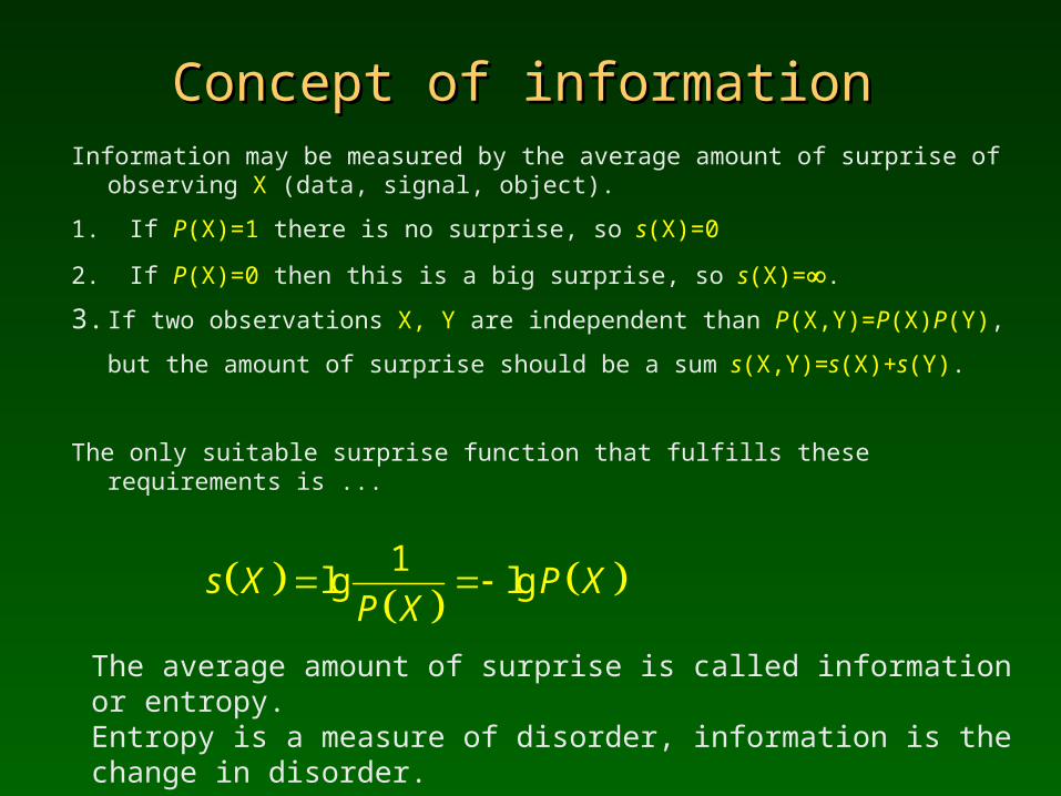
Concept of informationConcept of informationInformation may be measured by the average amount of surprise of

observing X (data, signal, object).

1. If P(X)=1 there is no surprise, so s(X)=0

2. If P(X)=0 then this is a big surprise, so s(X)=.

3. If two observations X, Y are independent than P(X,Y)=P(X)P(Y),

but the amount of surprise should be a sum s(X,Y)=s(X)+s(Y).

The only suitable surprise function that fulfills these requirements is ...

1lg lgs X P X

P X

The average amount of surprise is called information or entropy.Entropy is a measure of disorder, information is the change in disorder.

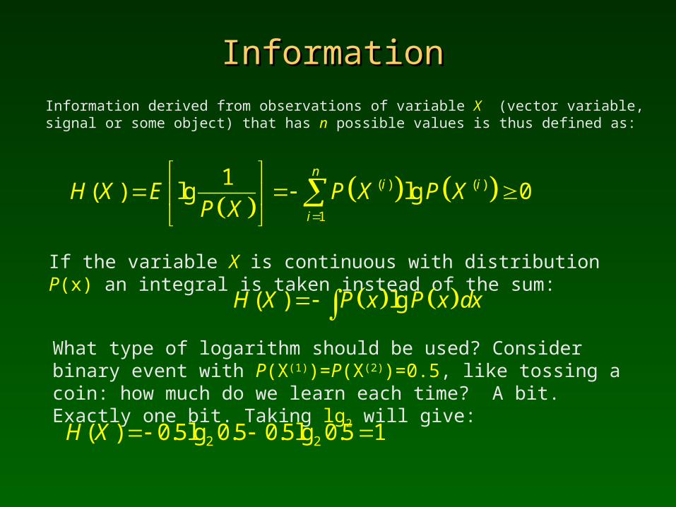
InformationInformation

Information derived from observations of variable X (vector variable, signal or some object) that has n possible values is thus defined as:

If the variable X is continuous with distribution P(x) an integral is taken instead of the sum:

( ) ( )

1

1( ) lg lg 0

ni i

i

H X E P X P XP X

What type of logarithm should be used? Consider binary event with P(X(1))=P(X(2))=0.5, like tossing a coin: how much do we learn each time? A bit. Exactly one bit. Taking lg2 will give:

( ) lgH X P x P x dx

2 2( ) 0.5lg 0.5 0.5lg 0.5 1H X

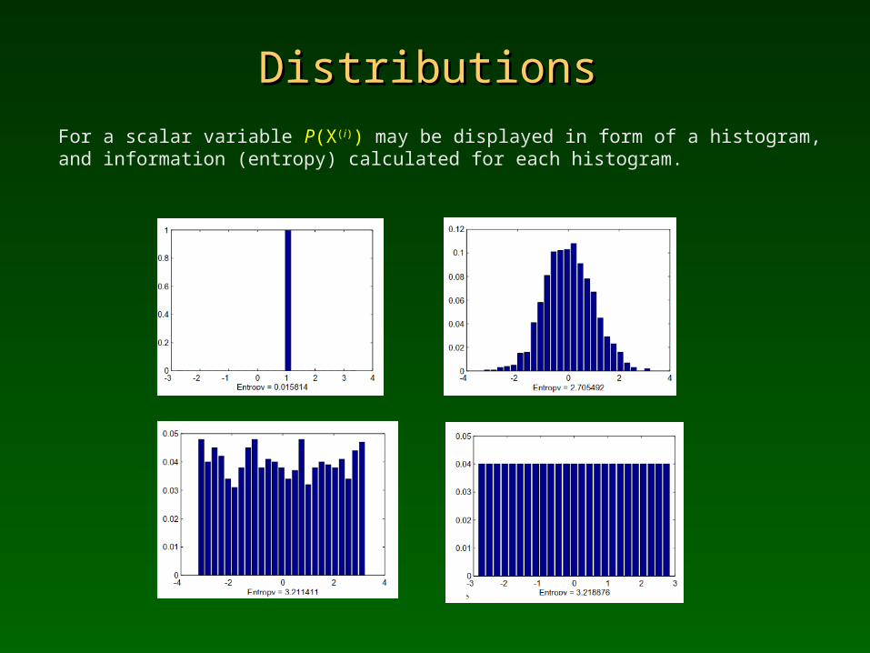
DistributionsDistributions

For a scalar variable P(X(i)) may be displayed in form of a histogram, and information (entropy) calculated for each histogram.

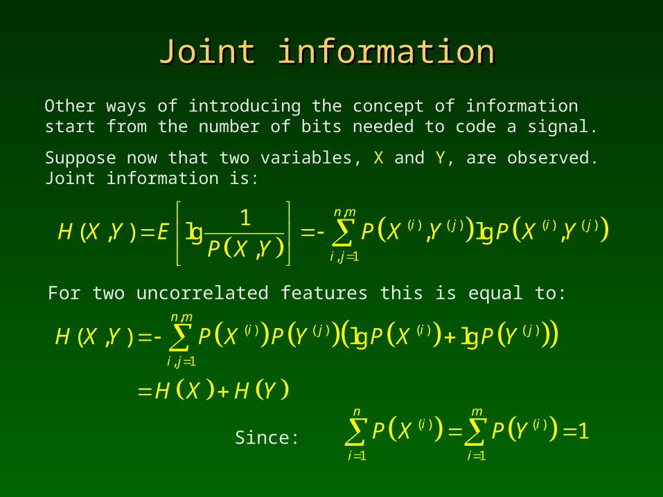
Joint informationJoint information

Other ways of introducing the concept of information start from the number of bits needed to code a signal.

Suppose now that two variables, X and Y, are observed. Joint information is:

For two uncorrelated features this is equal to:

,

( ) ( ) ( ) ( )

, 1

1( , ) lg , lg ,

,

n mi j i j

i j

H X Y E P X Y P X YP X Y

,( ) ( ) ( ) ( )

, 1

( , ) lg lgn m

i j i j

i j

H X Y P X P Y P X P Y

H X H Y

( ) ( )

1 1

1n m

i i

i i

P X P Y

Since:

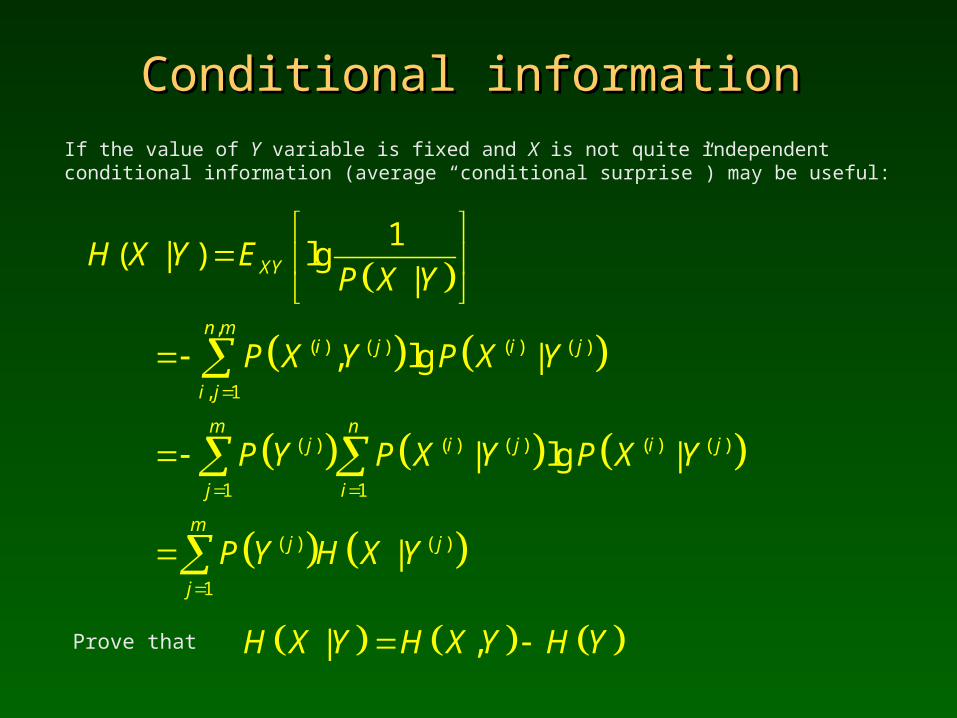
Conditional informationConditional information

If the value of Y variable is fixed and X is not quite independent conditional information (average “conditional surprise”) may be useful:

,( ) ( ) ( ) ( )

, 1

( ) ( ) ( ) ( ) ( )

1 1

( ) ( )

1

1( | ) lg

|

, lg |

| lg |

|

XY

n mi j i j

i j

m nj i j i j

j i

mj j

j

H X Y EP X Y

P X Y P X Y

P Y P X Y P X Y

P Y H X Y

Prove that | ,H X Y H X Y H Y

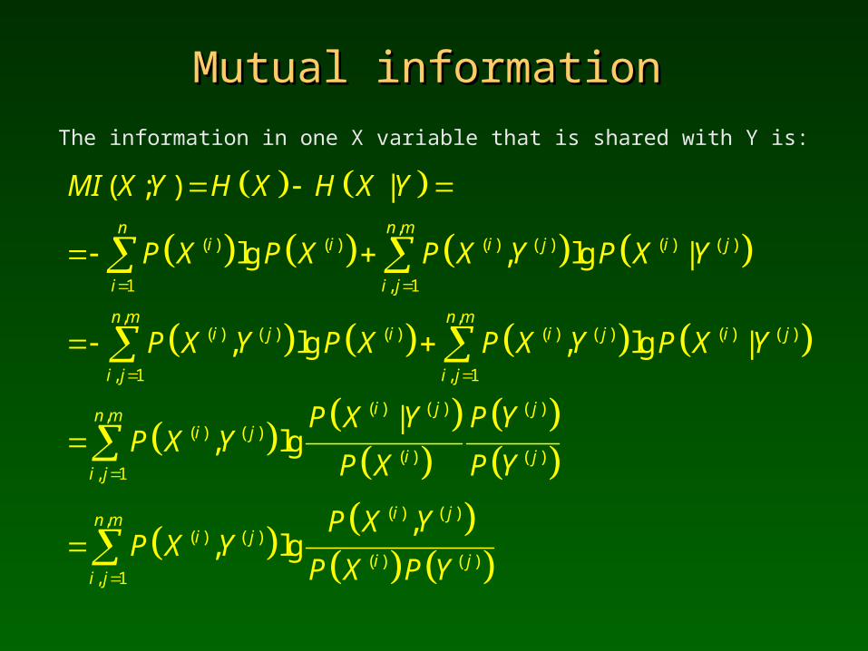
Mutual informationMutual information

The information in one X variable that is shared with Y is:

,( ) ( ) ( ) ( ) ( ) ( )

1 , 1

, ,( ) ( ) ( ) ( ) ( ) ( ) ( )

, 1 , 1

( ) ( ) ( ),( ) ( )

( ) ( ), 1

( ) ( )

( ) ( )

(

( ; ) |

lg , lg |

, lg , lg |

|, lg

,, lg

n mni i i j i j

i i j

n m n mi j i i j i j

i j i j

i j jn mi j

i ji j

i j

i j

MI X Y H X H X Y

P X P X P X Y P X Y

P X Y P X P X Y P X Y

P X Y P YP X Y

P X P Y

P X YP X Y

P X

,

) ( ), 1

n m

i ji j P Y

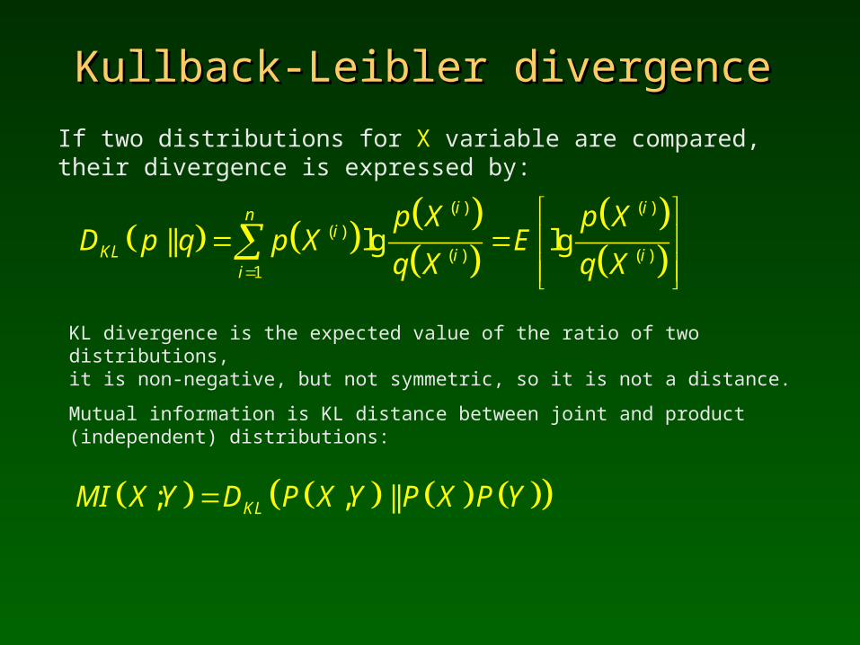
Kullback-Leibler divergenceKullback-Leibler divergence

If two distributions for X variable are compared, their divergence is expressed by:

( ) ( )

( )

( ) ( )1

|| lg lgi in

iKL i i

i

p X p XD p q p X E

q X q X

KL divergence is the expected value of the ratio of two distributions, it is non-negative, but not symmetric, so it is not a distance.

Mutual information is KL distance between joint and product (independent) distributions:

; , ||KLMI X Y D P X Y P X P Y

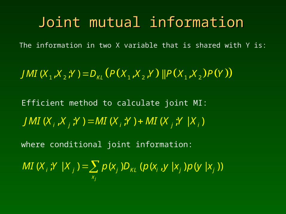
Joint mutual informationJoint mutual information

The information in two X variable that is shared with Y is:

1 2 1 2 1 2( , ; ) , , || ,KLJMI X X Y D P X X Y P X X P Y

( , ; ) ( ; ) ( ; | )i j i j iJMI X X Y MI X Y MI X Y X

Efficient method to calculate joint MI:

where conditional joint information:

( ; | ) ( ) ( ( , | ) ( | ))j

i j j KL i j jx

MI X Y X p x D p x y x p y x

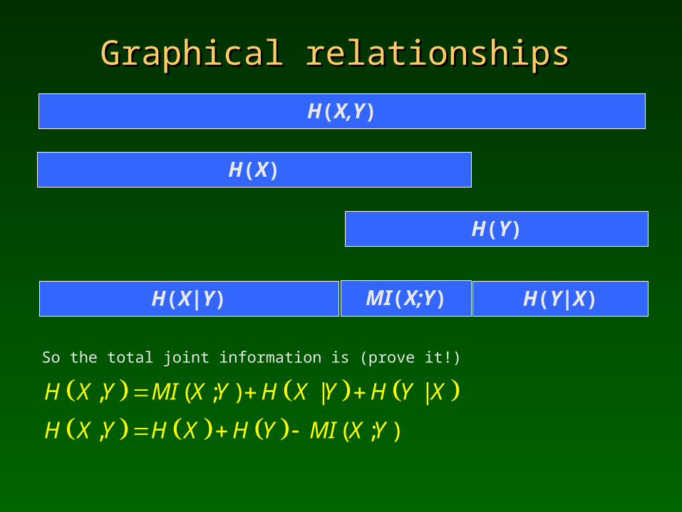
Graphical relationshipsGraphical relationships

H(X,Y)

So the total joint information is (prove it!)

H(X)

H(X|Y)

H(Y)

MI(X;Y) H(Y|X)

, ( ; ) | |

, ( ; )

H X Y MI X Y H X Y H Y X

H X Y H X H Y MI X Y

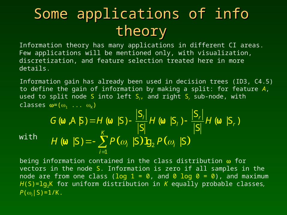
Some applications of info theorySome applications of info theory

Information theory has many applications in different CI areas. Few applications will be mentioned only, with visualization, discretization, and feature selection treated here in more details.

Information gain has already been used in decision trees (ID3, C4.5) to define the gain of information by making a split: for feature A, used to split node S into left Sl, and right Sr sub-node, with classes =(1 ... K)

S S( ,A|S) ( |S) ( |S ) ( |S )

S Sl r

l rG H H H ω ω ω ω

with

being information contained in the class distribution for vectors in the node S. Information is zero if all samples in the node are from one class (log 1 = 0, and 0 log 0 = 0), and maximum H(S)=lg2K for uniform distribution in K equally probable classes, P(i|S)=1/K.

21

( |S) |S lg |SK

i ii

H P P

ω

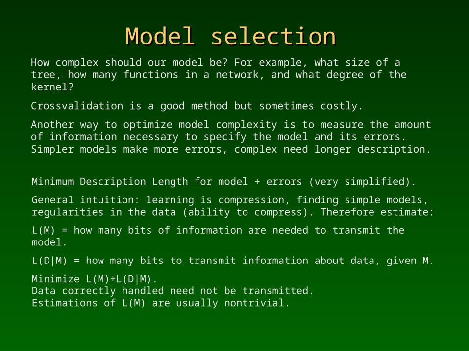
Model selectionModel selectionHow complex should our model be? For example, what size of a tree, how many functions in a network, and what degree of the kernel?

Crossvalidation is a good method but sometimes costly.

Another way to optimize model complexity is to measure the amount of information necessary to specify the model and its errors. Simpler models make more errors, complex need longer description.

Minimum Description Length for model + errors (very simplified).

General intuition: learning is compression, finding simple models, regularities in the data (ability to compress). Therefore estimate:

L(M) = how many bits of information are needed to transmit the model.

L(D|M) = how many bits to transmit information about data, given M.

Minimize L(M)+L(D|M). Data correctly handled need not be transmitted. Estimations of L(M) are usually nontrivial.

More on model selectionMore on model selection

Many criteria for information-based model selection have been devised in computational learning theory, two best known are:

AIC, Akaike Information Criterion. BIC, Bayesian Information Criterion.

The goal is to predict, using training data, which model has the best potential for accurate generalization.

Although model selection is a popular topic applications are relatively rare and selection via crossvalidation is commonly used.

Models may be trained by max. mutual information of outputs/classes:

This may in general be any non-linear transformation, for example implemented via basis set expansion methods.

( ) ( ); max ;i i

j jY g MI Y W

X W ω W

Visualization via max MI Visualization via max MI

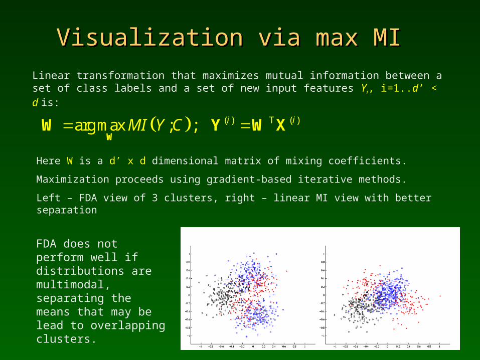
Linear transformation that maximizes mutual information between a set of class labels and a set of new input features Yi, i=1..d’ < d is:

Here W is a d’ x d dimensional matrix of mixing coefficients.

Maximization proceeds using gradient-based iterative methods.

Left – FDA view of 3 clusters, right – linear MI view with better separation

( ) T ( )arg max ; ; i iMI Y C W

W Y W X

FDA does not perform well if distributions are multimodal, separating the means that may be lead to overlapping clusters.

More examplesMore examples

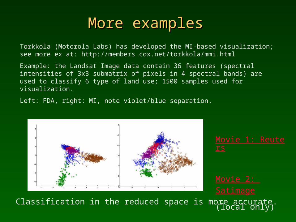
Torkkola (Motorola Labs) has developed the MI-based visualization;see more ex at: http://members.cox.net/torkkola/mmi.html

Example: the Landsat Image data contain 36 features (spectral intensities of 3x3 submatrix of pixels in 4 spectral bands) are used to classify 6 type of land use; 1500 samples used for visualization.

Left: FDA, right: MI, note violet/blue separation.

Classification in the reduced space is more accurate.

Movie 1: Reuters

Movie 2: Satimage

(local only)

Feature selection and attentionFeature selection and attention

• Attention: basic cognitive skill, without attention learning would not have been possible. First we focus on some sensation (visual object, sounds, smells, tactile sensations) and only then the full power of the brain is used to analyze this sensation.

• Given a large database, to find relevant information you may:

– discard features that do not contain information, – use weights to express their relative importance,– reduce dimensionality aggregating information, making linear or

non-linear combinations of subsets of features (FDA, MI) – new features may not be so understandable as the original ones.

– create new, more informative features, introducing new higher-level concepts; this is usually left to human invention.

Ranking and selectionRanking and selection

• Feature ranking: treat each feature as independent, and compare them to determine the order of relevance or importance (rank).

1 2 3 ...i i i idX X X X

Note that:

Several features may have identical relevance, especially for nominal features. This is either by chance, or because features are strongly correlated and therefore redundant.

Ranking depends on what we look for, for example rankings of cars from the comfort, usefulness in the city, or rough terrain performance point of view, will be quite different.

• Feature selection: search for the best subsets of features, remove redundant features, create subsets of one, two, k-best features.

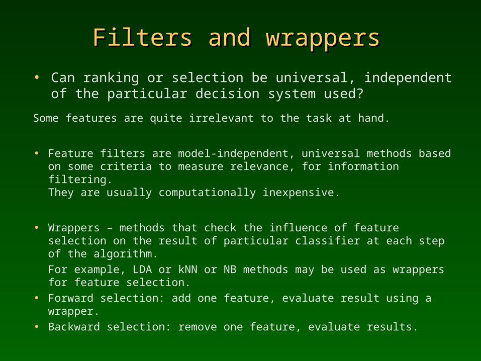
Filters and wrappersFilters and wrappers

• Can ranking or selection be universal, independent of the particular decision system used?

Some features are quite irrelevant to the task at hand.

• Feature filters are model-independent, universal methods based on some criteria to measure relevance, for information filtering. They are usually computationally inexpensive.

• Wrappers – methods that check the influence of feature selection on the result of particular classifier at each step of the algorithm.

For example, LDA or kNN or NB methods may be used as wrappers for feature selection.

• Forward selection: add one feature, evaluate result using a wrapper.

• Backward selection: remove one feature, evaluate results.

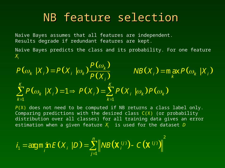
NB feature selectionNB feature selection

Naive Bayes assumes that all features are independent. Results degrade if redundant features are kept.

Naive Bayes predicts the class and its probability. For one feature Xi

| | kk i i k

i

PP X P X

P X

P(X) does not need to be computed if NB returns a class label only.Comparing predictions with the desired class C(X) (or probability distribution over all classes) for all training data gives an error estimation when a given feature Xi is used for the dataset D

max |i k ik

NB X P X

1 1

| 1 |K K

k i i i k kk k

P X P X P X P

2

( ) ( )1

1

arg min |n

j ji i

ij

i E X D NB C

X X

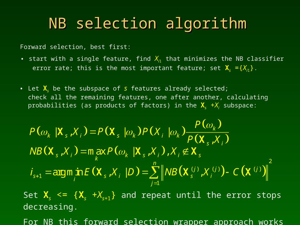
NB selection algorithmNB selection algorithm

Forward selection, best first:

• start with a single feature, find Xi1 that minimizes the NB classifier

error rate; this is the most important feature; set Xs ={Xi1}.

Set Xs <= {Xs +Xs+1} and repeat until the error stops decreasing.

For NB this forward selection wrapper approach works quite well.

• Let Xs be the subspace of s features already selected;

check all the remaining features, one after another, calculating probabilities (as products of factors) in the Xs +Xi subspace:

| , | |,k

k s i s k i ks i

PP X P P X

P X

X X

X , max | , ,s i k s i i s

kNB X P X X X X X

2

( ) ( ) ( )1

1

arg min , | ,n

j j js s i s i

ij

i E X D NB X C

X X X

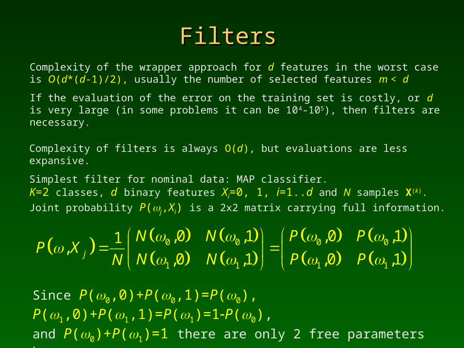
FiltersFiltersComplexity of the wrapper approach for d features in the worst case is O(d*(d-1)/2), usually the number of selected features m < d

If the evaluation of the error on the training set is costly, or d is very large (in some problems it can be 104-105), then filters are necessary.

Since P(0,0)+P(0,1)=P(0), P(1,0)+P(1,1)=P(1)=1P(0), and P(0)+P(1)=1 there are only 2 free parameters here.

Complexity of filters is always O(d), but evaluations are less expansive.

Simplest filter for nominal data: MAP classifier.K=2 classes, d binary features Xi=0, 1, i=1..d and N samples X(k).

Joint probability P(j,Xi) is a 2x2 matrix carrying full information.

0 0 0 0

1 1 1 1

,0 ,1 ,0 ,11,

,0 ,1 ,0 ,1j

N N P PP X

N N P PN

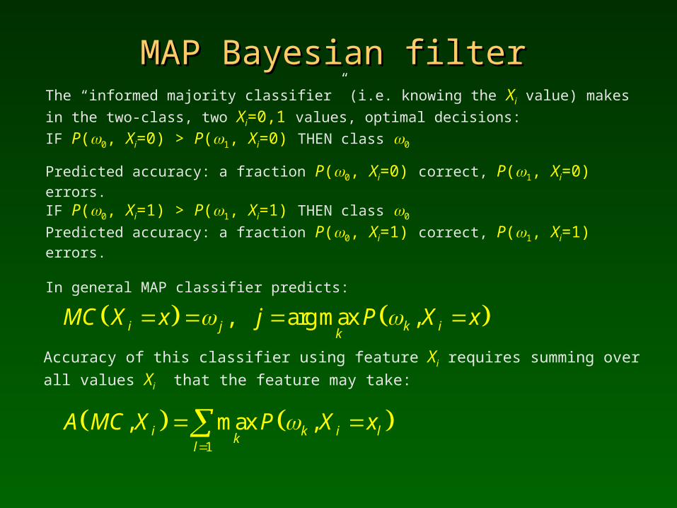
MAP Bayesian filterMAP Bayesian filterThe “informed majority classifier” (i.e. knowing the Xi value) makes in the

two-class, two Xi=0,1 values, optimal decisions:

IF P(0, Xi=0) > P(1, Xi=0) THEN class 0

Predicted accuracy: a fraction P(0, Xi=0) correct, P(1, Xi=0) errors.

IF P(0, Xi=1) > P(1, Xi=1) THEN class 0

Predicted accuracy: a fraction P(0, Xi=1) correct, P(1, Xi=1) errors.

In general MAP classifier predicts:

Accuracy of this classifier using feature Xi requires summing over all values Xi

that the feature may take:

, arg max ,i j k ik

MC X x j P X x

1

, max ,i k i lk

l

A MC X P X x

MC MC propertiesproperties

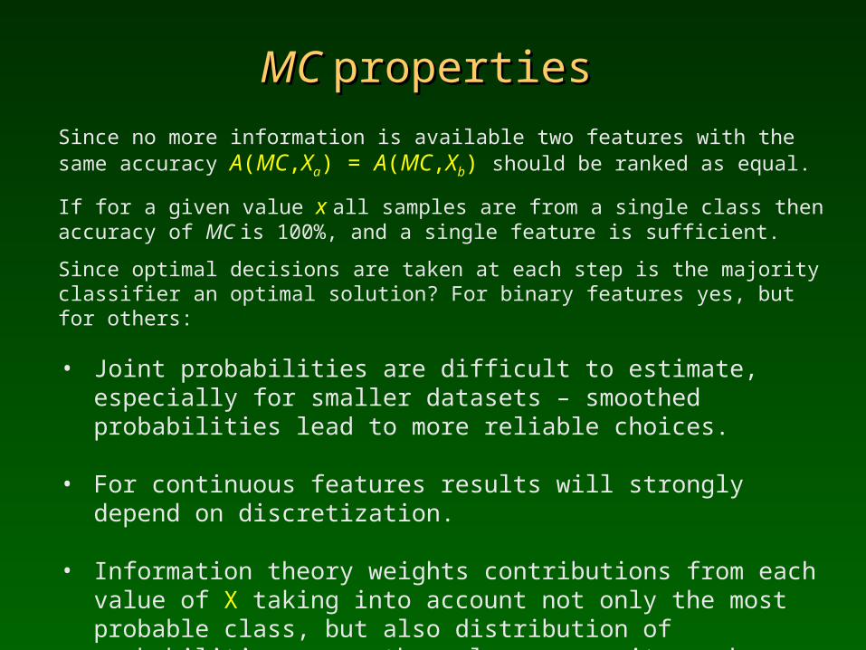
Since no more information is available two features with the same accuracy A(MC,Xa) = A(MC,Xb) should be ranked as equal.

If for a given value x all samples are from a single class then accuracy of MC is 100%, and a single feature is sufficient.

Since optimal decisions are taken at each step is the majority classifier an optimal solution? For binary features yes, but for others:

• Joint probabilities are difficult to estimate, especially for smaller datasets – smoothed probabilities lead to more reliable choices.

• For continuous features results will strongly depend on discretization.

• Information theory weights contributions from each value of X taking into account not only the most probable class, but also distribution of probabilities over other classes, so it may have some advantages, especially for continuous features.

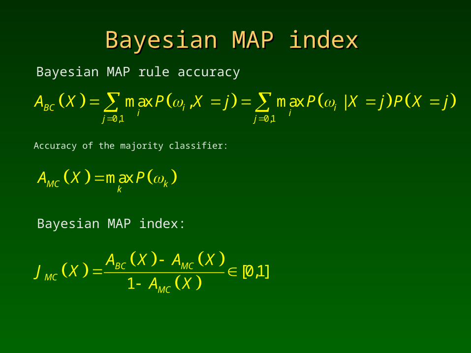
Bayesian MAP indexBayesian MAP indexBayesian MAP rule accuracy

Accuracy of the majority classifier:

0,1 0,1

max , max |BC i ii i

j j

A X P X j P X j P X j

maxMC kk

A X P

Bayesian MAP index:

[0,1]1

BC MCMC

MC

A X A XJ X

A X

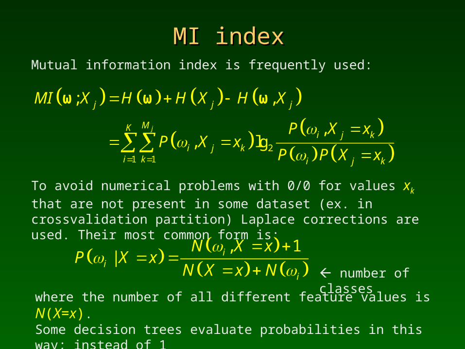
MI indexMI indexMutual information index is frequently used:

To avoid numerical problems with 0/0 for values xk that are not present in

some dataset (ex. in crossvalidation partition) Laplace corrections are used. Their most common form is:

2

1 1

; ,

,, lg

j

j j j

MKi j k

i j ki k i j k

MI X H H X H X

P X xP X x

P P X x

ω ω ω

, 1| i

ii

N X xP X x

N X x N

where the number of all different feature values is N(X=x). Some decision trees evaluate probabilities in this way; instead of 1 and N(i) other values may be used as long as probabilities sum to 1.

number of classes

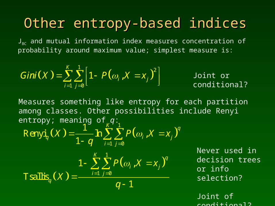
Other entropy-based indicesOther entropy-based indicesJBC and mutual information index measures concentration of probability around maximum value; simplest measure is:

Measures something like entropy for each partition among classes. Other possibilities include Renyi entropy; meaning of q:

1 2

1 0

1 ,K

i ji j

Gini X P X x

1

1 0

1Renyi ln ,

1

K q

q i ji j

X P X xq

1

1 0

1 ,

Tsallis1

K q

i ji j

q

P X x

Xq

Never used in decision treesor info selection?

Joint of conditional?

Joint or conditional?

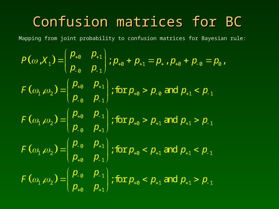
Confusion matrices for BCConfusion matrices for BCMapping from joint probability to confusion matrices for Bayesian rule:

0 11 0 1 0 0 0

0 1

0 11 2 0 0 1 1

0 1

0 11 2 0 1 1 1

0 1

0 11 2 0 1 1 1

0 1

0 11 2

, ; , ,

, ; for and

, ; for and

, ; for and

,

p pP X p p p p p p

p p

p pF p p p p

p p

p pF p p p p

p p

p pF p p p p

p p

p pF

p

0 1 1 10 1

; for andp p p pp

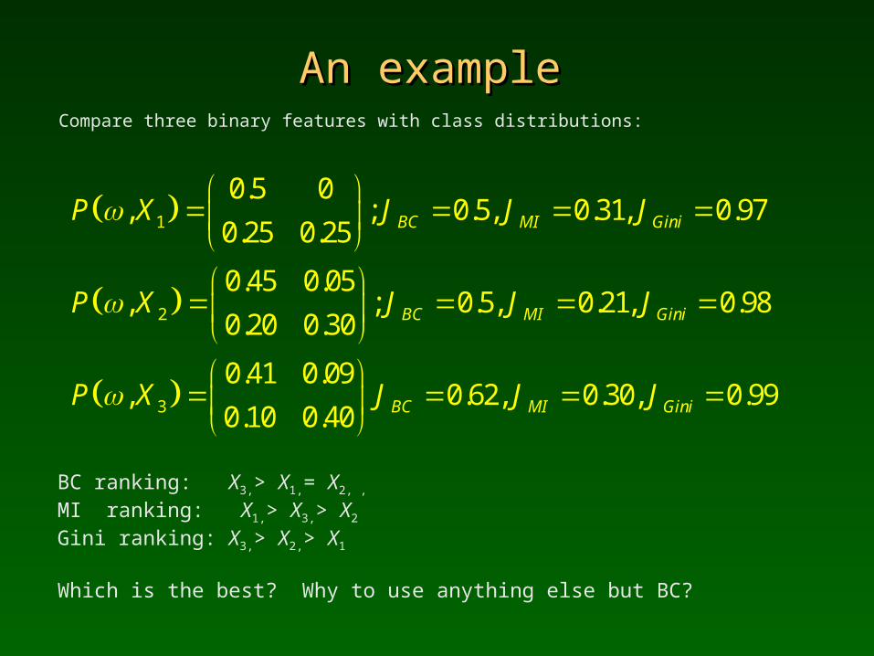
An exampleAn exampleCompare three binary features with class distributions:

1

2

3

0.5 0, ; 0.5, 0.31, 0.97

0.25 0.25

0.45 0.05, ; 0.5, 0.21, 0.98

0.20 0.30

0.41 0.09, 0.62, 0.30, 0.99

0.10 0.40

BC MI Gini

BC MI Gini

BC MI Gini

P X J J J

P X J J J

P X J J J

BC ranking: X3,> X1,= X2, , MI ranking: X1,> X3,> X2

Gini ranking: X3,> X2,> X1

Which is the best? Why to use anything else but BC?

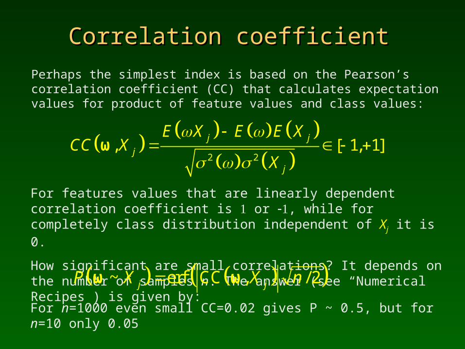
Correlation coefficientCorrelation coefficient

Perhaps the simplest index is based on the Pearson’s correlation coefficient (CC) that calculates expectation values for product of feature values and class values:

For features values that are linearly dependent correlation coefficient is or , while for completely class distribution independent of Xj it is 0.

How significant are small correlations? It depends on the number of samples n. The answer (see “Numerical Recipes”) is given by:

2 2

, [ 1, 1]j j

j

j

E X E E XCC X

X

ω

~ erf CC , / 2j jP X X nω ω

For n=1000 even small CC=0.02 gives P ~ 0.5, but for n=10 only 0.05

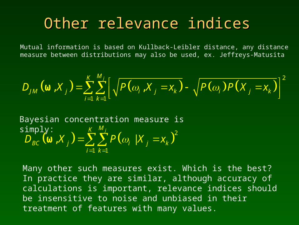
Other relevance indicesOther relevance indices

Mutual information is based on Kullback-Leibler distance, any distance measure between distributions may also be used, ex. Jeffreys-Matusita

Bayesian concentration measure is simply:

2

1 1

, ,jMK

JM j i j k i j ki k

D X P X x P P X x

ω

Many other such measures exist. Which is the best? In practice they are similar, although accuracy of calculations is important, relevance indices should be insensitive to noise and unbiased in their treatment of features with many values.

2

1 1

, |jMK

BC j i j ki k

D X P X x

ω

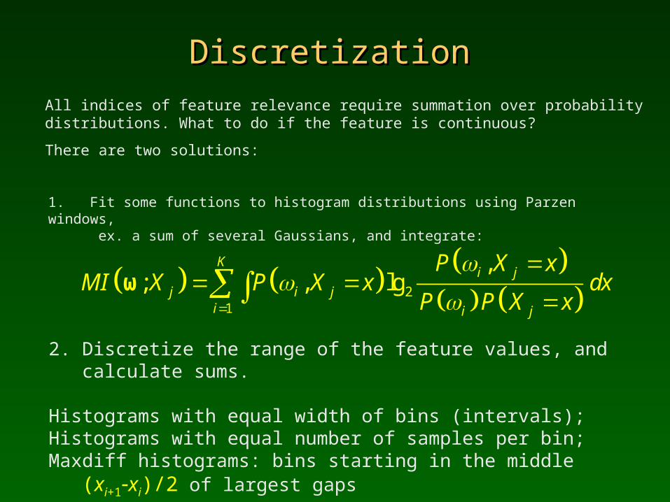
DiscretizationDiscretization

All indices of feature relevance require summation over probability distributions. What to do if the feature is continuous?

There are two solutions:

2. Discretize the range of the feature values, and calculate sums.

Histograms with equal width of bins (intervals);Histograms with equal number of samples per bin;Maxdiff histograms: bins starting in the middle (xi+1xi)/2 of largest gaps

V-optimal: sum of variances in bins should be minimal (difficult).

2

1

,; , lg

Ki j

j i ji i j

P X xMI X P X x dx

P P X x

ω

1. Fit some functions to histogram distributions using Parzen windows, ex. a sum of several Gaussians, and integrate:

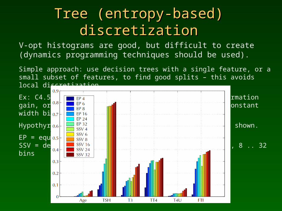
Tree (entropy-based) discretizationTree (entropy-based) discretization

V-opt histograms are good, but difficult to create (dynamics programming techniques should be used).

Simple approach: use decision trees with a single feature, or a small subset of features, to find good splits – this avoids local discretization.

Ex: C4.5 decision tree discretization maximizing information gain, or SSV tree based separability criterion, vs. constant width bins.

Hypothyroid screening data, 5 continuous features, MI shown.

EP = equal width partition; SSV = decision tree partition (discretization) into 4, 8 .. 32 bins

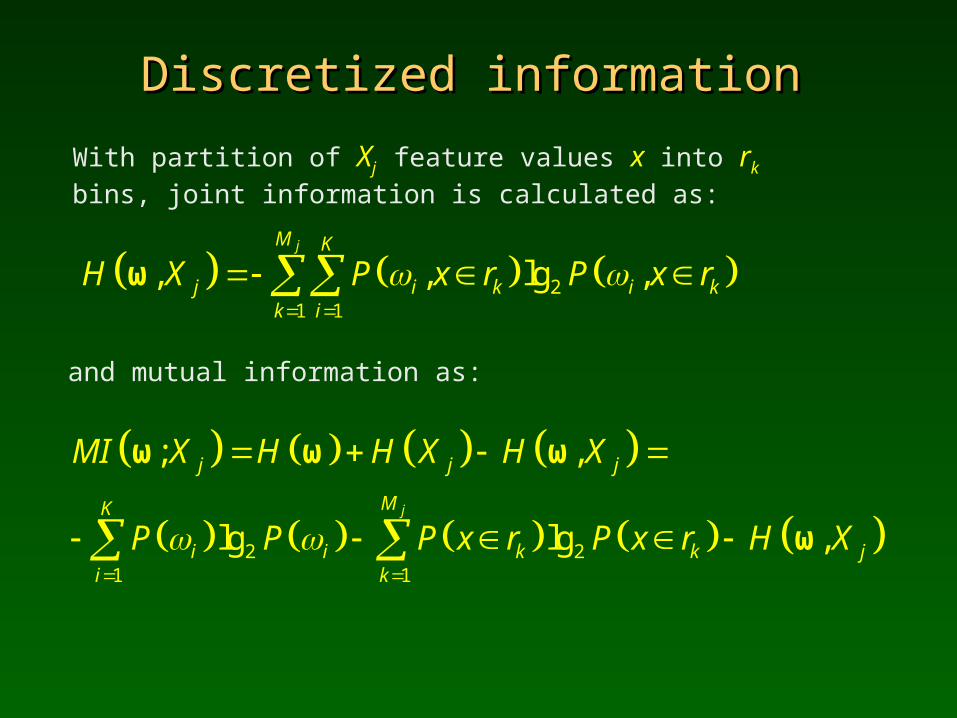
Discretized informationDiscretized information

With partition of Xj feature values x into rk bins, joint information is

calculated as:

and mutual information as:

21 1

, , lg ,jM K

j i k i kk i

H X P x r P x r

ω

2 21 1

; ,

lg lg ,j

j j j

MK

i i k k ji k

MI X H H X H X

P P P x r P x r H X

ω ω ω

ω

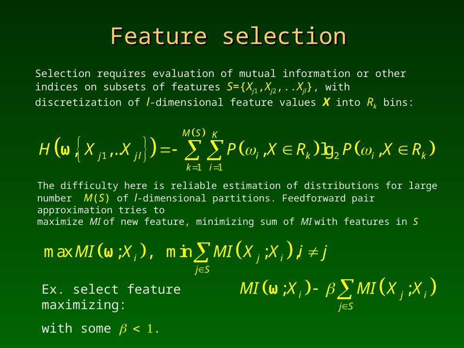
Feature selectionFeature selection

Selection requires evaluation of mutual information or other indices on subsets of features S={Xj1,Xj2,..Xjl}, with discretization of l-dimensional

feature values X into Rk bins:

The difficulty here is reliable estimation of distributions for large number M(S) of l-dimensional partitions. Feedforward pair approximation tries to maximize MI of new feature, minimizing sum of MI with features in S

1 21 1

, ,.. , lg ,M S K

j j l i k i kk i

H X X P X R P X R

ω

max ; , min ; ,i j ij S

MI X MI X X i j

ω

Ex. select feature maximizing:

with some .

; ;i j ij S

MI X MI X X

ω

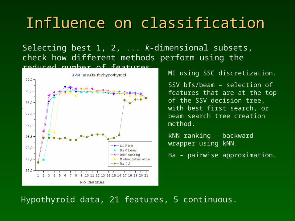
Influence on classificationInfluence on classification

Selecting best 1, 2, ... k-dimensional subsets, check how different methods perform using the reduced number of features.

MI using SSC discretization.

SSV bfs/beam – selection of features that are at the top of the SSV decision tree, with best first search, or beam search tree creation method.

kNN ranking – backward wrapper using kNN.

Ba – pairwise approximation.

Hypothyroid data, 21 features, 5 continuous.

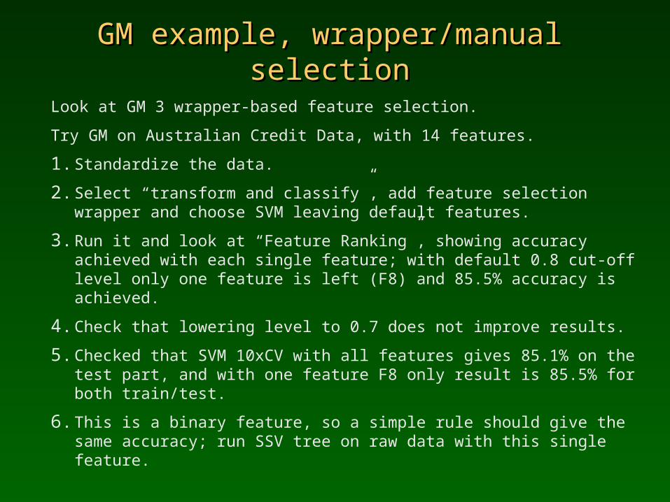
GM example, wrapper/manual selectionGM example, wrapper/manual selection

Look at GM 3 wrapper-based feature selection.

Try GM on Australian Credit Data, with 14 features.

1. Standardize the data.

2. Select “transform and classify”, add feature selection wrapper and choose SVM leaving default features.

3. Run it and look at “Feature Ranking”, showing accuracy achieved with each single feature; with default 0.8 cut-off level only one feature is left (F8) and 85.5% accuracy is achieved.

4. Check that lowering level to 0.7 does not improve results.

5. Checked that SVM 10xCV with all features gives 85.1% on the test part, and with one feature F8 only result is 85.5% for both train/test.

6. This is a binary feature, so a simple rule should give the same accuracy; run SSV tree on raw data with this single feature.

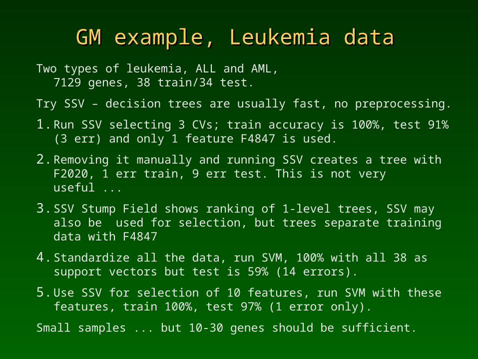
GM example, Leukemia dataGM example, Leukemia data

Two types of leukemia, ALL and AML, 7129 genes, 38 train/34 test.

Try SSV – decision trees are usually fast, no preprocessing.

1. Run SSV selecting 3 CVs; train accuracy is 100%, test 91% (3 err) and only 1 feature F4847 is used.

2. Removing it manually and running SSV creates a tree with F2020, 1 err train, 9 err test. This is not very useful ...

3. SSV Stump Field shows ranking of 1-level trees, SSV may also be used for selection, but trees separate training data with F4847

4. Standardize all the data, run SVM, 100% with all 38 as support vectors but test is 59% (14 errors).

5. Use SSV for selection of 10 features, run SVM with these features, train 100%, test 97% (1 error only).

Small samples ... but 10-30 genes should be sufficient.