Computational Intelligence: Computational Intelligence: Methods and ApplicationsMethods and Applications

Lecture 12

Bayesian decisions: foundation of learning

Włodzisław Duch

Dept. of Informatics, UMK

Google: W Duch

LearningLearningLearningLearning• Learning from data requires a model of data.

• Traditionally parametric models of different phenomena were developed in science and engineering; parametric models are easy to interpret, so if the phenomenon is simple enough and a theory exist construct a model and use algorithmic approach.

• Empirical non-parametric modeling is data driven, goal oriented. It dominates in biological systems. Learn from data!

• Given some examples = training data, create a model of data that answers specific question, estimating those characteristics of the data that may be useful to make future predictions.

• Learning = estimate parameters of the (non-parametric) model; paradoxically, non-parametric models have a lot of parameters.

• Many other approaches to learning exist, but no time to explore ...

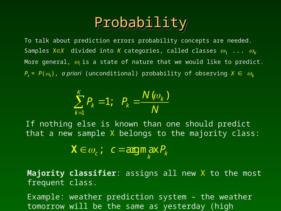
ProbabilityProbabilityProbabilityProbabilityTo talk about prediction errors probability concepts are needed.

Samples XX divided into K categories, called classes 1 ... K

More general, i is a state of nature that we would like to predict.

Pk = P(k), a priori (unconditional) probability of observing X k

1

( )1;

Kk

k kk

NP P

N

If nothing else is known than one should predict that a new sample X belongs to the majority class:

; arg maxc kk

c P X

Majority classifier: assigns all new X to the most frequent class.

Example: weather prediction system – the weather tomorrow will be the same as yesterday (high accuracy prediction!).

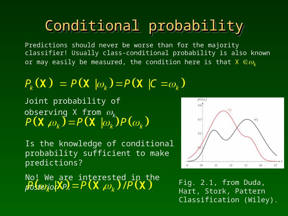
Conditional probabilityConditional probabilityConditional probabilityConditional probabilityPredictions should never be worse than for the majority classifier! Usually class-conditional probability is also known or may easily be

measured, the condition here is that X k

| | k k kP P P C X X X

Joint probability of observing X from k

Is the knowledge of conditional probability sufficient to make predictions?

No! We are interested in the posterior P.

, | k k kP P P X X

| , / k kP P P X X X Fig. 2.1, from Duda, Hart, Stork, Pattern Classification (Wiley).

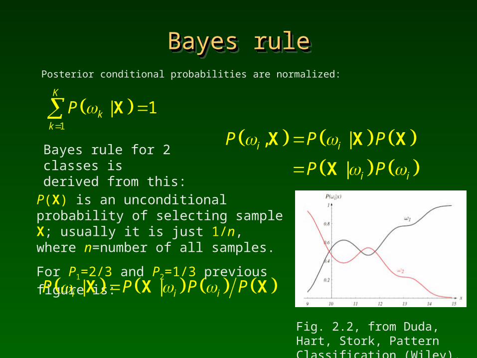
Bayes ruleBayes ruleBayes ruleBayes rulePosterior conditional probabilities are normalized:

Bayes rule for 2 classes isderived from this:

P(X) is an unconditional probability of selecting sample X; usually it is just 1/n, where n=number of all samples.

For P1=2/3 and P2=1/3 previous figure is:

1

| 1K

kk

P

X

, |

|

i i

i i

P P P

P P

X X X

X

| |i i iP P P P X X X

Fig. 2.2, from Duda, Hart, Stork, Pattern Classification (Wiley).

Bayes decisionsBayes decisionsBayes decisionsBayes decisionsBayes decision: given a sample X select class 1 if:

Probability of an error is:

Average error is:

1 2| |P P X X

1 2| min | , |P P P X X X

| |P E P P P d

X X X X

Bayes decision rule minimizes average error selecting smallest P(|X)

Using Bayes rule and multiplying both sides by P(X):

1 1 2 2| |P P P P X X

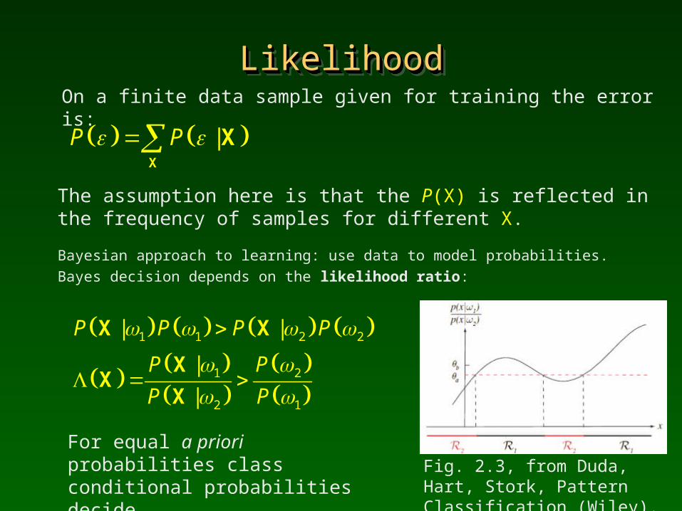
LikelihoodLikelihoodLikelihoodLikelihood

Bayesian approach to learning: use data to model probabilities.

Bayes decision depends on the likelihood ratio:

For equal a priori probabilities class conditional probabilities decide.

On a finite data sample given for training the error is:

|P P X

X

The assumption here is that the P(X) is reflected in the frequency of samples for different X.

1 1 2 2

1 2

2 1

| |

|

|

P P P P

P P

P P

X X

XX

X

Fig. 2.3, from Duda, Hart, Stork, Pattern Classification (Wiley).

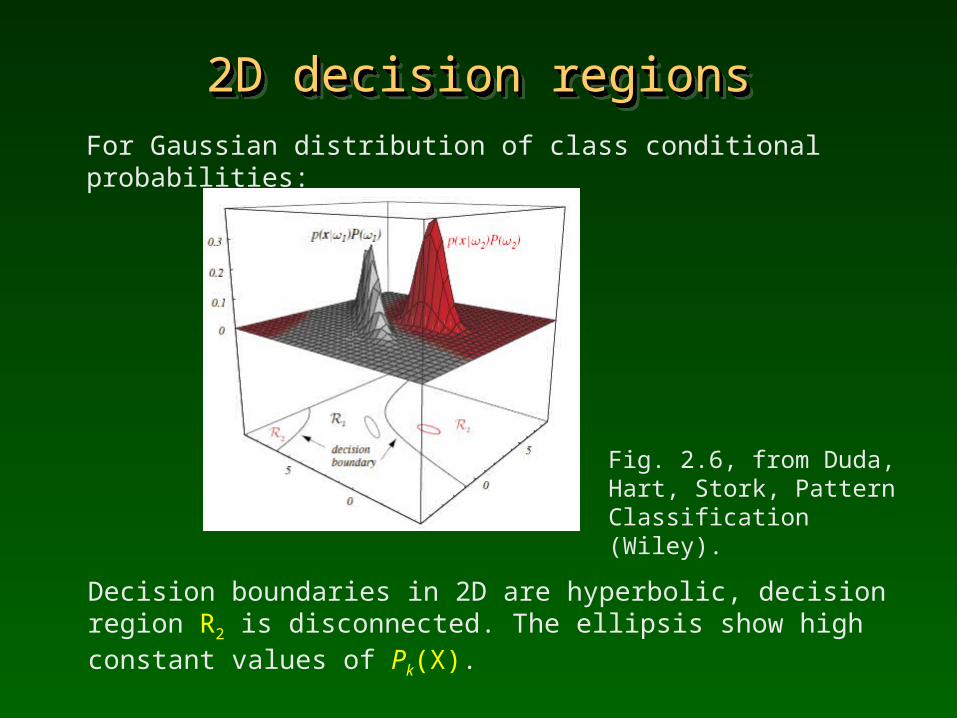
2D decision regions2D decision regions2D decision regions2D decision regionsFor Gaussian distribution of class conditional probabilities:

Decision boundaries in 2D are hyperbolic, decision region R2 is disconnected. The ellipsis show high constant values of Pk(X).

Fig. 2.6, from Duda, Hart, Stork, Pattern Classification (Wiley).

ExampleExampleExampleExample

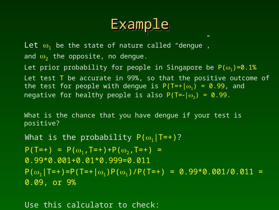
Let 1 be the state of nature called “dengue”,

and 2 the opposite, no dengue.

Let prior probability for people in Singapore be P(1)=0.1%

Let test T be accurate in 99%, so that the positive outcome of the test for people with dengue is P(T=+|1) = 0.99, and negative for healthy people is also P(T=|2) = 0.99.

What is the chance that you have dengue if your test is positive?

What is the probability P(1|T=+)?

P(T=+) = P(1,T=+)+P(2,T=+) = 0.99*0.001+0.01*0.999=0.011

P(1|T=+)=P(T=+|1)P(1)/P(T=+) = 0.99*0.001/0.011 = 0.09, or 9%

Use this calculator to check:

http://StatPages.org/bayes.html

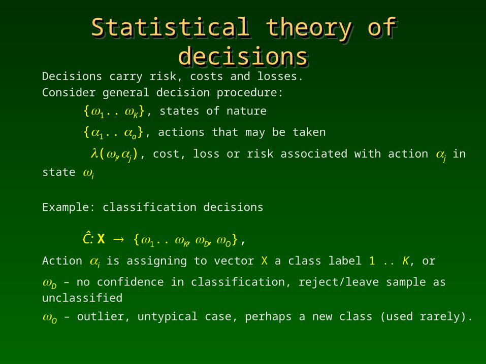
Statistical theory of decisionsStatistical theory of decisionsStatistical theory of decisionsStatistical theory of decisionsDecisions carry risk, costs and losses.

Consider general decision procedure:

{1.. K}, states of nature

{1.. a}, actions that may be taken

(i,j), cost, loss or risk associated with action j in state i

Example: classification decisions

Ĉ: X {1.. K, D, O},

Action i is assigning to vector X a class label 1 .. K, or

D – no confidence in classification, reject/leave sample as unclassified

O – outlier, untypical case, perhaps a new class (used rarely).

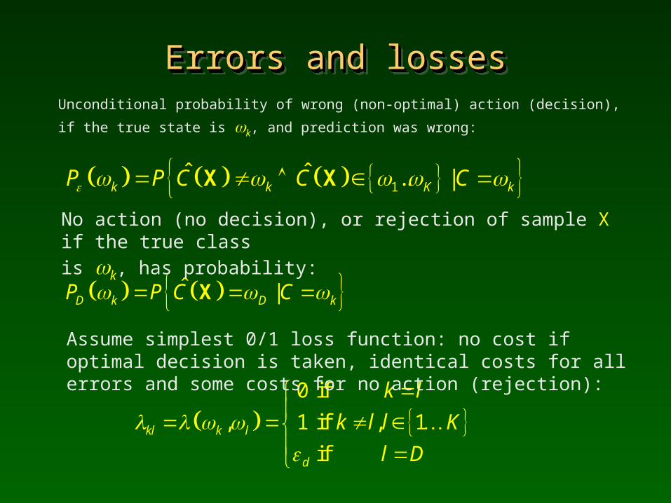
Errors and lossesErrors and lossesErrors and lossesErrors and lossesUnconditional probability of wrong (non-optimal) action (decision),

if the true state is k, and prediction was wrong:

1ˆ ˆ .. |k k K kP P C C C X X

ˆ |D k D kP P C C X

No action (no decision), or rejection of sample X if the true class

is k, has probability:

0 if

, 1 if , 1

ifkl k l

d

k l

k l l K

l D

Assume simplest 0/1 loss function: no cost if optimal decision is taken, identical costs for all errors and some costs for no action (rejection):

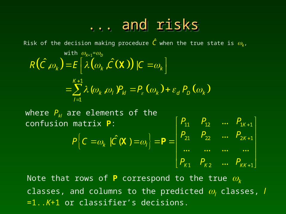
... and risks... and risks... and risks... and risksRisk of the decision making procedure Ĉ when the true state is k,

with K+1=D

where Pkl are elements of the confusion matrix P:

1

1

ˆ ˆ, , |

( , )

k k k

K

k l kl k d D kl

R C E C C

P P P

X

11 12 1 1

21 22 2 1

1 2 1

...

...ˆ| ( )... ... ... ...

...

K

Kk l

K K KK

P P P

P P PP C C

P P P

X P

Note that rows of P correspond to the true k classes, and columns to

the predicted l classes, l =1..K+1 or classifier’s decisions.

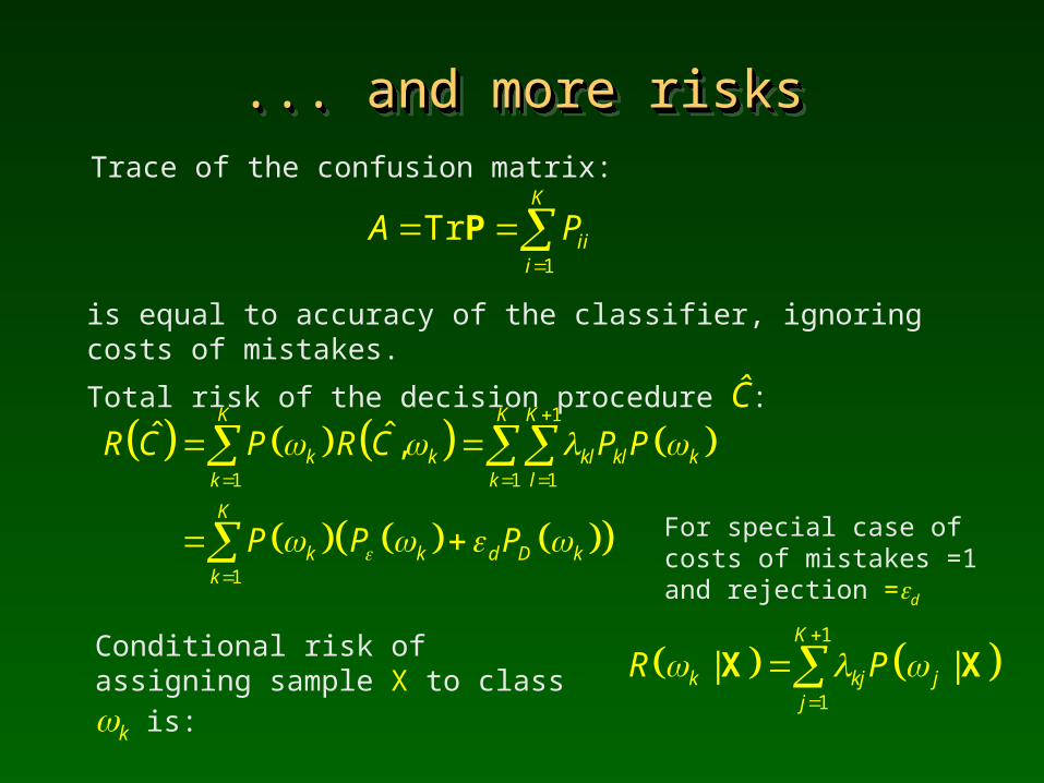
... and more risks... and more risks... and more risks... and more risksTrace of the confusion matrix:

is equal to accuracy of the classifier, ignoring costs of mistakes.

Total risk of the decision procedure Ĉ:

1

Tr K

iii

A P

P

1

1 1 1

1

ˆ ˆ ,K K K

k k kl kl kk k l

K

k k d D kk

R C P R C P P

P P P

1

1

| |K

k kj jj

R P

X XConditional risk of assigning sample X

to class k is:

For special case of costs of mistakes =1 and rejection =d