Computational Materials Theory and

Methods

Alexey V. AkimovUniversity at Buffalo, SUNY

1

Lecture 2: Classical Molecular Mechanics

2

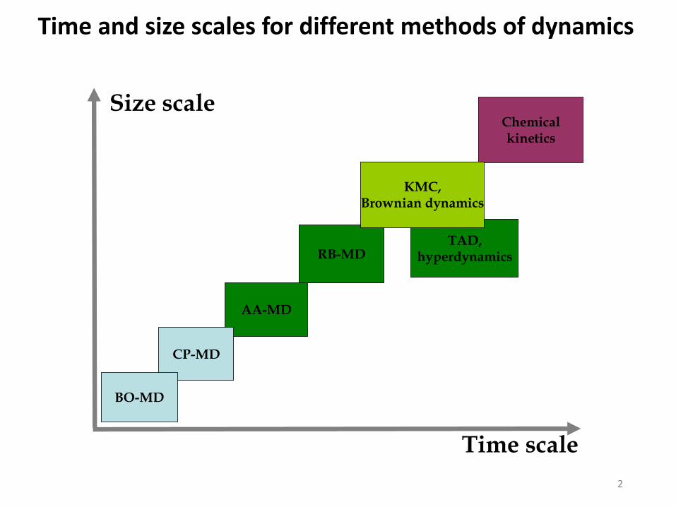
AA-MD

RB-MD

Chemicalkinetics

CP-MD

BO-MD

Time scale

Size scale

TAD,hyperdynamics

KMC,Brownian dynamics

Time and size scales for different methods of dynamics

CASSCF

HF

DFT

Class I force field

CG-modelsStatistical

mechanicalmodels

Reactive force field

Level of coarse-graining

Level of theory

Analytic

polarizable force field

Full CI

Class II force field

QM/MM

3

Accuracy and methodology

4

Potential energy surface (PES)

𝑯𝚿 𝒓;𝑹 = 𝑬 𝑹 𝚿(𝐫; 𝐑)

Stationary Schrodinger Equation

𝑹

𝑬(𝑹)

• Computationally expensive!• Can we fit the curves with a

simple analytical function?

Within the Born-Oppenheimer Approximation

5

𝑬𝒕𝒐𝒕 = 𝑬𝒃𝒐𝒏𝒅𝒆𝒅 + 𝑬𝒏𝒐𝒏−𝒃𝒐𝒏𝒅𝒆𝒅

Force fields (Molecular Mechanics)

Force field

functional parameters

𝒇(𝒒𝟏, 𝒒𝟐, . . 𝒒𝑵; 𝑷𝟏, 𝑷𝟐, …𝑷𝑴)

• Numerically efficient• Has suitable derivatives• Is continuous • Physically meaningfull

• Based on atom and interaction types• Minimal amount is desirable• Transferable or system-specific• Reproduce ab initio or experiment

(thermodynamic properties, spectra,chemical reactivity, etc.)

describes covalent bonding non-covalent interactions

6

bonded, 4-particle: torsion/dihedral, out-of-plane/improper dihedrals

bonded, 3-particle: angle bending

bonded, 2-particle: bond stretching

𝑬𝒃𝒐𝒏𝒅𝒆𝒅 = 𝑬𝒃𝒐𝒏𝒅𝒔 + 𝑬𝒂𝒏𝒈𝒍𝒆𝒔 + 𝑬𝒅𝒊𝒉𝒆𝒅𝒓𝒂𝒍𝒔 + 𝑬𝒐𝒐𝒑

Bonded interactions

In quantum mechanics: bonds are everywhere “bond order”In molecular mechanics: bonded atoms must be specified by the user

non-bonded2-particlevdw and Coulombinteractions

7

Non-bonded interactions

Charges are usually constant,but there are geometry-dependentcharge schemes (e.g. qEQ)Accounts for the polarizability

In periodic systems, the latticesummation methods are used,such as Ewald sum method.

Rappe, A. K.; Goddard, W. A. J. Phys. Chem. 1991, 95, 3358–3363.

Ogawa, T.; Kurita, N.; Sekino, H.; Kitao, O.; Tanaka, S. Chem. Phys. Lett. 2004, 397, 382–387.

Karasawa, N.; Goddard III, W. A. J. Phys. Chem. 1989, 93, 7320–7327.

Chen, J.; Martinez, T. J. Chem. Phys. Lett. 2007, 438, 315–320.

8

Atom types

Rappe, A. K.; Casewit, C. J.; Colwell, K. S.; Goddard III, W. A.; Skiff, W. M. J. Am. Chem. Soc. 1992, 114, 10024–10035.

Wang, J.; Wolf, R. M.; Caldwell, J. W.; Kollman, P. A.; Case, D. A. J. Comput. Chem. 2004, 25, 1157–1174.

Generalized Amber FFUniversal FF (UFF)

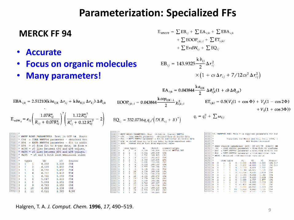
Halgren, T. A. J. Comput. Chem.1996, 17, 490–519.

MERCK FF 94

General purpose FFs Specialized FFs

9

Parameterization: Specialized FFs

MERCK FF 94

• Accurate• Focus on organic molecules• Many parameters!

Halgren, T. A. J. Comput. Chem. 1996, 17, 490–519.

10

Rappe, A. K.; Casewit, C. J.; Colwell, K. S.; Goddard III, W. A.; Skiff, W. M. J. Am. Chem. Soc. 1992, 114, 10024–10035.

Universal FF (UFF)

Parameterization: General-purpose FFs

• Not so accurate!• General purpose (e.g. organometallic)• Way fewer parameters!

11

Polarization: Charge equilibration method

Rappe, A. K.; Goddard, W. A. J. Phys. Chem. 1991, 95, 3358–3363.

electronegativity

self-Coloumb(idempotential)

12

Handling vdW interactions with PBC

𝑈 𝑹 , 𝑳𝒙, 𝑳𝒚, 𝑳𝒛 =1

2

𝑛𝑥,𝑛𝑦𝑛𝑧

𝑖,𝑗

𝑈( 𝑹𝒊 − 𝑹𝒋 − 𝑳𝒙𝑛𝑥 − 𝑳𝒚𝑛𝑦 − 𝑳𝒛𝑛𝑧 )

𝑳𝒙, 𝑳𝒚, 𝑳𝒛 Simulation cell vectors

𝑹 Atomic coordinates

• All combinations of integers 𝑛𝑥, 𝑛𝑦 , 𝑛𝑧• That is an infinite number of cells!• Exclude self-interactions

Dealing with the infinite number of terms

𝑹

𝑬(𝑹)𝑹𝒄𝒖𝒕 Van der Walls interactions

are short-ranged

Disregard all the interactionsfor the particles separated more than by 𝑅𝑐𝑢𝑡

𝑈 𝑟 = 4𝜖𝜎

𝑟

12

−𝜎

𝑟

6

13

Simulation cell Periodic Image

Same atom/molecule

1 2 3 1’ 2’ 3’3’’2’’

𝑹𝒄𝒖𝒕

Handling non-bonded interactions with PBC

If simulation cell size 𝑳 is larger than 𝟐𝑹𝒄𝒖𝒕, it is sufficient to have only one shell of periodic images

14

𝑹

𝑬(𝑹)

Electrostatic interactionsare long-ranged

Can not use the cutoff technique

Direct summation is slowly converging

Handling electrostatic interactions with PBC

𝑈 𝑟 = 𝐶𝑞𝑖𝑞𝑗

𝑟

𝟏

𝒓=𝐞𝐫𝐟 𝒄(𝒓)

𝒓+𝟏 − 𝒆𝒓𝒇𝒄(𝒓)

𝒓

Converges fastin real space

Converges fastin reciprocal space

15

Continuity of forces

offon

off

onoff

on

onoff

on

onoff

off

on

offon RRR

RR

RR

RR

RR

RR

RR

RR

RR

RRRSW

,

.0

631

,1

,,

23

Truncation of the potential makes it discontinuous at 𝑅 = 𝑅𝑐𝑢𝑡.

Solution: shift by the corresponding energy

shifted potential

But the forces are still discontinuous!

Solution: Modify the potential such that

the force is also continuous at 𝑅 = 𝑅𝑐𝑢𝑡

shifted-force potential

potential

force

Class I FFs: (diagonal terms): e.g. all bonds, all angles, etc.Class II FFs: (+ cross-terms): e.g. add bond-angle interactions (e.g. like in MMFF94)

16

Classification of the FFs

𝐸 𝑞1, 𝑞2, … = 𝐸 0, 0, … +

𝑖∈𝐷𝑂𝐹

𝜕𝐸

𝜕𝑞𝑖𝑞𝑖 +

1

2

𝑖,𝑗∈𝐷𝑂𝐹

𝜕2𝐸

𝜕𝑞𝑖𝜕𝑞𝑗𝑞𝑖𝑞𝑗 +⋯

Bond-order (“reactive”) FFs:

𝐸 𝑞1, 𝑞2, … =

(𝑖,𝑗)

𝑎𝑖𝑗𝑏𝑜𝑖𝑗 + (𝑖1,𝑗1),(𝑖2,𝑗2)

𝑎𝑖1𝑗1𝑎2𝑗2𝑏𝑜𝑖1𝑗1𝑏𝑜𝑖2𝑗2 +⋯

𝑏𝑜𝑖𝑗 = 𝐴𝑒−𝛼𝑟𝑖𝑗 Bond order

not the way it is defined in QM!

17

Reactive FFs

𝑹

𝑬(𝑹)Why bond order?

𝑼(𝒙) =𝟏

𝟐𝒌𝒙𝟐

Bond breaking is impossible!

Harmonic potential:

𝑼 𝒙 = 𝑫 𝒆−𝟐𝜶 𝒓𝒊𝒋−𝒓𝒊𝒋

𝟎

− 𝟐𝒆−𝜶 𝒓𝒊𝒋−𝒓𝒊𝒋

𝟎

= 𝑫[𝒃𝒐𝒊𝒋𝟐 − 𝟐𝒃𝒐𝒊𝒋]

Physically correct limit: No interaction for infinitely separated atoms

Morse potential:

𝑈 𝑥 → ∞ → ∞

𝑏𝑜𝑖𝑗 = 𝐴𝑒−𝛼𝑟𝑖𝑗

𝐴 = 𝑒𝛼𝑟𝑖𝑗0

𝑈 𝑥 → ∞ → 0

Bond breaking is possible!

18

ReaxFF

van Duin, A. C. T.; Dasgupta, S.; Lorant, F.; Goddard, W. A. J. Phys. Chem. A 2001, 105, 9396–9409.

ij

surfacejmoleculeiji

rr

ijchem rSWeDE ijij

,

2

110

ij

surfacejmoleculeiji ij

ij

ij

ij

ijnonbondedphys rSWrr

DE

,

612

, 2

Physisorption: All atoms, except S

Chemisorption: S atom

b=2.878 Å

19

Constructing your own FF: Example 1

𝑅𝑜𝑛 = 2 3𝑏

𝑅𝑜𝑓𝑓 = 5𝑏

The temperature when 𝐶𝑛, 𝑛 ≥ 2 started rotatingdidn’t depend too much on the alkyl size 𝑛

20

Akimov, A. V.; Williams, C.; Kolomeisky, A. B. J. Phys. Chem. C2012, 116, 13816–13826.

Constructing your own FF: Example 2

Parameterization (PM6) Validation C60/Au diffusion coefficients

21

Materials modeling FFs

Akimov, A. V.; Prezhdo, O. V. Chem. Rev. 2015, 115, 5797–5890.

Embedded atom method (EAM) Systems with non-directional bonds (metals, alloys)

Modified EAM (MEAM) Introduced bond directionality (silicon, etc.)

MEAM92 Extended set of elements (metals and non-metals)

Brenner, Tersoff-Brenner, REBOReactive potentials for hydrocarbons

ReaxFF

Charge-optimized many-body (COMBx) Polarizable reactive potentials

Learn more:

Daw, M. S.; Baskes, M. I. Phys. Rev. Lett. 1983, 50, 1285−1288

Baskes, M. I. Phys. Rev. Lett. 1987, 59, 2666−2669Baskes, M. I.; Nelson, J. S.; Wright, A. F. Phys. Rev. B 1989, 40, 6085−6100.

Baskes, M. I. Phys. Rev. B 1992, 46, 2727−2742.

Brenner, D. W. Phys. Rev. B 1990, 42, 9458−9471

Van Duin, A. C. T.; Dasgupta, S.; Lorant, F.; Goddard, W. A. J. Phys. Chem. A 2001, 105, 9396−9409

Yu, J.; Sinnott, S.; Phillpot, S. Phys. Rev. B 2007, 75, 085311

22

Exercises: Running AA MD of H2O cluster

params["input_structure"] = "/23waters-aa.ent"

First, we cool the system down -optimization

T = 300 K time = 5 ps

Tut2.1

T = 200 K

T = 100 K

Then, put some kinetic energy

23

Exercises: Running RB MD of H2O cluster

params["input_structure"] = "/23waters.ent"

Now, do the same, but remove internal degrees of freedom

Tut2.1

Using rigid-body moleculardynamics (RB-MD)

T = 100 K T = 200 K

Internal degrees of freedomact as “energy buffer”

The kinetics in AA and RBbay be very different!

𝑬𝒕𝒐𝒕 = 𝑬𝒃𝒐𝒏𝒅𝒆𝒅 + 𝑬𝒏𝒐𝒏−𝒃𝒐𝒏𝒅𝒆𝒅

24

Exercises: Running aa MD of SubPc/C60 cluster

Tut2.2This is the same as before, but using a predefined library Use: run_aa_md.py

High T – behaves wildlyEnergy is well conserved

Optimized 10 ps of MD

Internal degrees of freedom“absorb” energy leadingto low temperature

Assign T = 300 K after cooling

25

Exercises: Running aa MD of SubPc/C60 cluster

Tut2.2This is the same as before, but using another classUse: run_aa_md_state.py

Gives the same as before (NVE ensemble)

ST.set_thermostat(therm)

"ensemble":"NVT"10 ps of MD

One N center inversion occurs

26

Tut2.3

Exercises: Computing specific heat capacity of gold

0.129 𝑱

𝒈∗𝑲

𝐶𝑉 =4.72∗10−4 𝐻𝑎2

3.17 ∗ 10−6𝐻𝑎𝐾 ∗ 278.02𝐾2

= 1.93 ∗ 10−3𝐻𝑎

𝐾

𝑚 =216

𝑁𝐴𝑚𝑜𝑙 ∗ 197

𝑔

𝑚𝑜𝑙=42552

𝑁𝐴𝑔 = 7.07 ∗ 10−20𝑔

𝑐 =𝐶𝑣𝑚

=1.93 ∗ 10−3

𝐻𝑎𝐾

7.07 ∗ 10−20𝑔∗ 4.36 ∗ 10−18

𝐽

𝐻𝑎= 1.19 ∗ 10−1 = 𝟎. 𝟏𝟏𝟗

𝑱

𝒈 ∗ 𝑲

Reference value:

m m

27

𝑞1 𝑞2

𝑇 =1

2m ሶ𝑞1

2 + ሶ𝑞22

V = k q1 − q22

𝑑

𝑑𝑡

𝜕𝐿

𝜕 ሶ𝑞𝑖−𝜕𝐿

𝜕𝑞𝑖= 0

𝑚 ሷ𝑞1 = −2𝑘 𝑞1 − 𝑞2

𝑑

𝑑𝑡

𝜕𝐿

𝜕 ሶ𝑞𝑖=𝜕𝐿

𝜕𝑞𝑖= −

𝜕𝑉

𝜕𝑞𝑖

𝑚 ሷ𝑞2 = 2𝑘 𝑞1 − 𝑞2

𝑑𝑒𝑡 2𝑘 − 𝑚𝜔2 −2𝑘−2𝑘 2𝑘 − 𝑚𝜔2 = 2𝑘 −𝑚𝜔2 2 − 4k2 = −4km𝜔2 +𝑚2𝜔4 = 0

𝑚𝜔2 = 4𝑘 ⇒ 𝜔 = 2𝑘

𝑚

Normal modes analysis

m mM

28

𝑞1 𝑞2 𝑞3

𝑞𝑖 are the displacements of all atoms in Cartesian coordinate system

𝑇 =1

2m ሶ𝑞1

2 + ሶ𝑞32 +

1

2𝑀 ሶ𝑞2

2 Kinetic energy

U =1

2k q1 − q2

2 +1

2𝑘 𝑞3 − 𝑞2

2 Potential energy

Normal modes analysis

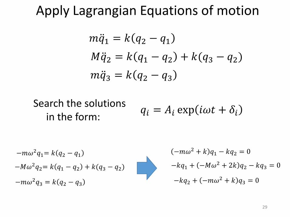
Search the solutionsin the form:

29

Apply Lagrangian Equations of motion

𝑚 ሷ𝑞1 = 𝑘 𝑞2 − 𝑞1

𝑀 ሷ𝑞2 = 𝑘 𝑞1 − 𝑞2 + 𝑘(𝑞3 − 𝑞2)

𝑚 ሷ𝑞3 = 𝑘 𝑞2 − 𝑞3

𝑞𝑖 = 𝐴𝑖 exp 𝑖𝜔𝑡 + 𝛿𝑖

−𝑚𝜔2𝑞1= 𝑘 𝑞2 − 𝑞1

−𝑀𝜔2𝑞2= 𝑘 𝑞1 − 𝑞2 + 𝑘(𝑞3 − 𝑞2)

−𝑚𝜔2𝑞3 = 𝑘 𝑞2 − 𝑞3

−𝑚𝜔2 + 𝑘 𝑞1 − 𝑘𝑞2 = 0

−𝑘𝑞1 + −𝑀𝜔2 + 2𝑘 𝑞2 − 𝑘𝑞3 = 0

−𝑘𝑞2 + −𝑚𝜔2 + 𝑘 𝑞3 = 0

30

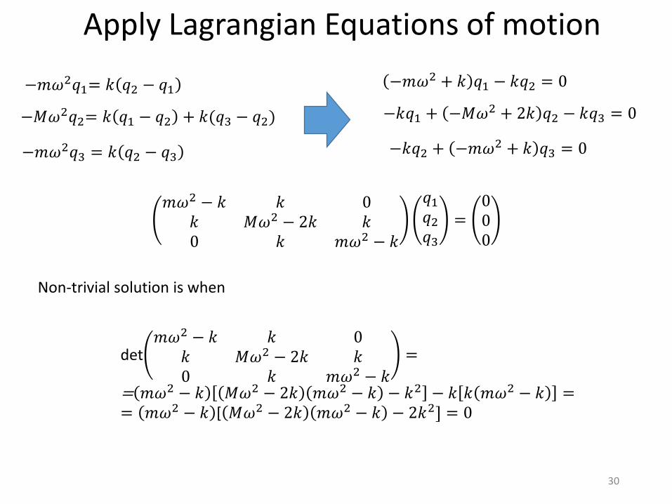
Apply Lagrangian Equations of motion

−𝑚𝜔2𝑞1= 𝑘 𝑞2 − 𝑞1

−𝑀𝜔2𝑞2= 𝑘 𝑞1 − 𝑞2 + 𝑘(𝑞3 − 𝑞2)

−𝑚𝜔2𝑞3 = 𝑘 𝑞2 − 𝑞3

−𝑚𝜔2 + 𝑘 𝑞1 − 𝑘𝑞2 = 0

−𝑘𝑞1 + −𝑀𝜔2 + 2𝑘 𝑞2 − 𝑘𝑞3 = 0

−𝑘𝑞2 + −𝑚𝜔2 + 𝑘 𝑞3 = 0

𝑚𝜔2 − 𝑘 𝑘 0𝑘 𝑀𝜔2 − 2𝑘 𝑘0 𝑘 𝑚𝜔2 − 𝑘

𝑞1𝑞2𝑞3

=000

det𝑚𝜔2 − 𝑘 𝑘 0

𝑘 𝑀𝜔2 − 2𝑘 𝑘0 𝑘 𝑚𝜔2 − 𝑘

=

= 𝑚𝜔2 − 𝑘 𝑀𝜔2 − 2𝑘 𝑚𝜔2 − 𝑘 − 𝑘2 − 𝑘 𝑘 𝑚𝜔2 − 𝑘 == 𝑚𝜔2 − 𝑘 [ 𝑀𝜔2 − 2𝑘 𝑚𝜔2 − 𝑘 − 2𝑘2] = 0

Non-trivial solution is when

Normal modes

(translation)

31

𝑀𝜔2 − 2𝑘 𝑚𝜔2 − 𝑘 − 2𝑘2 = 𝑀𝑚𝜔4 − 2𝑘𝑚𝜔2 − 𝑘𝑀𝜔2 = 𝜔2 𝑀𝑚𝜔2 − 𝑘 2𝑚 +𝑀

Possible solutions

𝜔1 = 0

𝜔2 =𝑘

𝑚

𝜔3 =𝑘 2𝑚 +𝑀

𝑀𝑚

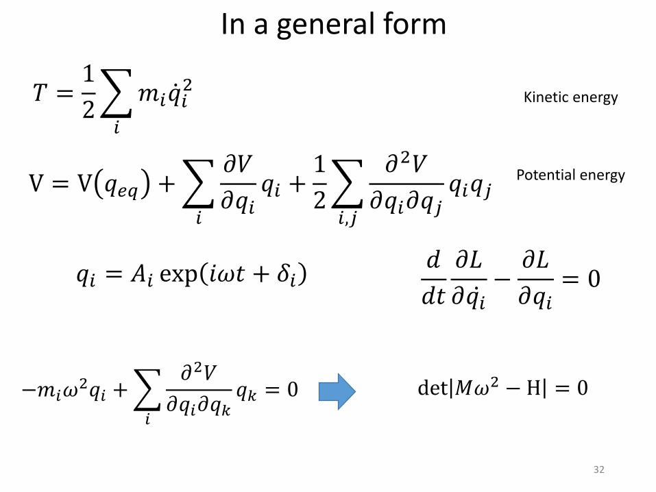
𝑇 =1

2

𝑖

𝑚𝑖 ሶ𝑞𝑖2

Kinetic energy

V = V 𝑞𝑒𝑞 +

𝑖

𝜕𝑉

𝜕𝑞𝑖𝑞𝑖 +

1

2

𝑖,𝑗

𝜕2𝑉

𝜕𝑞𝑖𝜕𝑞𝑗𝑞𝑖𝑞𝑗

Potential energy

In a general form

𝑞𝑖 = 𝐴𝑖 exp 𝑖𝜔𝑡 + 𝛿𝑖𝑑

𝑑𝑡

𝜕𝐿

𝜕 ሶ𝑞𝑖−𝜕𝐿

𝜕𝑞𝑖= 0

−𝑚𝑖𝜔2𝑞𝑖 +

𝑖

𝜕2𝑉

𝜕𝑞𝑖𝜕𝑞𝑘𝑞𝑘 = 0 det 𝑀𝜔2 − H = 0

32