Computational Methods forManagement and Economics

Carla Gomes

Module 6c

Initialization in Simplex (Textbook – Hillier and Lieberman)

Initialization

Adapting to other forms

• Equality constraints

• Negative Right-hand sides

• Constraints ≥• Minimization

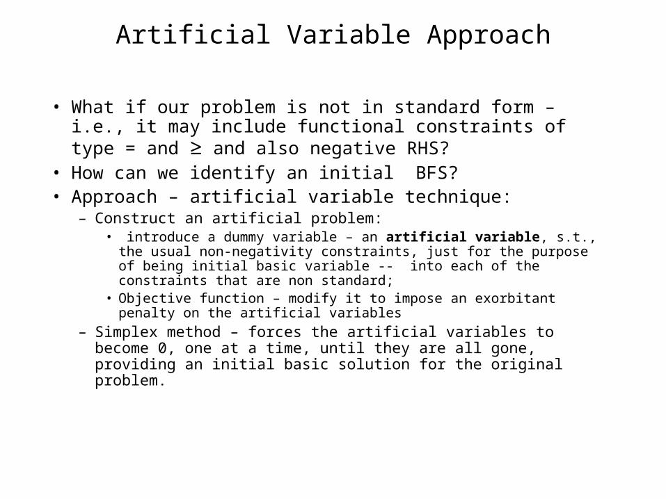
Artificial Variable Approach

• What if our problem is not in standard form – i.e., it may include functional constraints of type = and ≥ and also negative RHS?

• How can we identify an initial BFS?• Approach – artificial variable technique:

– Construct an artificial problem:• introduce a dummy variable – an artificial variable, s.t., the usual non-

negativity constraints, just for the purpose of being initial basic variable -- into each of the constraints that are non standard;

• Objective function – modify it to impose an exorbitant penalty on the artificial variables

– Simplex method – forces the artificial variables to become 0, one at a time, until they are all gone, providing an initial basic solution for the original problem.

Handling Equality Constraints

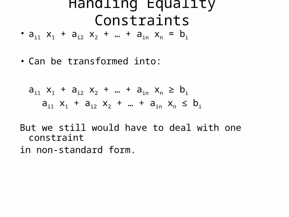
• ai1 x1 + ai2 x2 + … + ain xn = bi

• Can be transformed into:

ai1 x1 + ai2 x2 + … + ain xn ≥ bi

ai1 x1 + ai2 x2 + … + ain xn ≤ bi

But we still would have to deal with one constraint in non-standard form.

Wyndor Glass

• Requirement: plant 3must be uses at full capacity 3 x1 + 2 x2 = 18;

• Algebraic form:

Z - 3 x1 - 2 x2 = 0;

x1 + x3 = 4;

2 x2 + x3 = 12;

3 x1 + 2 x2 = 18;

What’s the problem with this initial system from the simplex’s point of view?

Coefficients of Variables

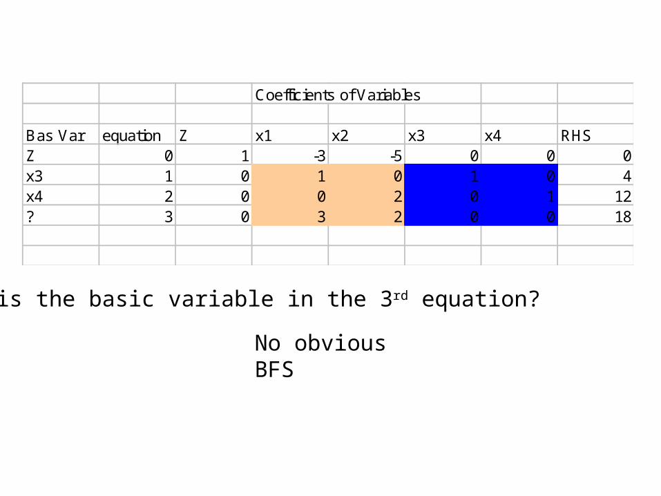
Bas Var equation Z x1 x2 x3 x4 RHSZ 0 1 -3 -5 0 0 0x3 1 0 1 0 1 0 4x4 2 0 0 2 0 1 12? 3 0 3 2 0 0 18

What is the basic variable in the 3rd equation?

No obvious BFS

ProcedureConstruct an artificial problem that has the same optimal solution as the real problem by making two modifications tothe real problem:1. Apply the artificial variable technique by introducing a non-negative artificial

variable into the equality constraint as if it were a slack variable.

2. Assign an overwhelming penalty to having by changing the objective function to:

5x3 x1 + 2 x2 + = 18;

05x

Z = 3 x1 + 2 x2 - M 5

x

M is a huge positive number (Big M Method).

185x

5x = 18 - 3 x1 + 2 x2

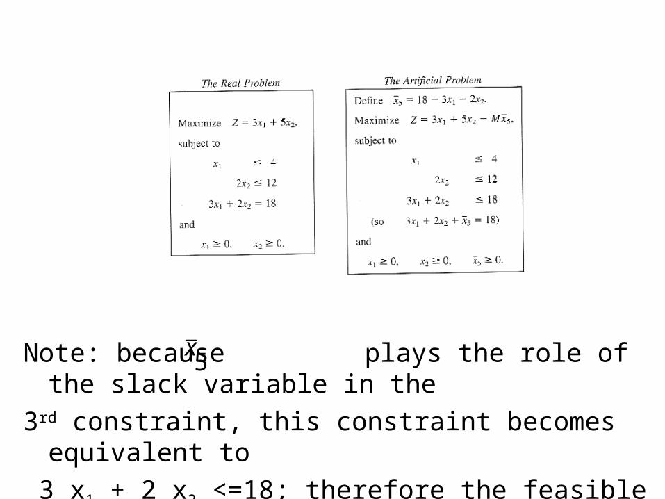
Note: because plays the role of the slack variable in the

3rd constraint, this constraint becomes equivalent to

3 x1 + 2 x2 <=18; therefore the feasible region is identical to

the feasible region of the original Wyndor Glass problem.

5x

3. Converting Z equation into proper form

x1 + x3 = 4;

2 x2 + x4 = 12;

3 x1 + 2 x2 + = 18;

Is this form the right form for the simplex? Why?

Z - 3 x1 - 2 x2 + M = 0 5

x

convert Z equation into the proper form by subtracting

from Eq(0), Eq(3) times M

5x

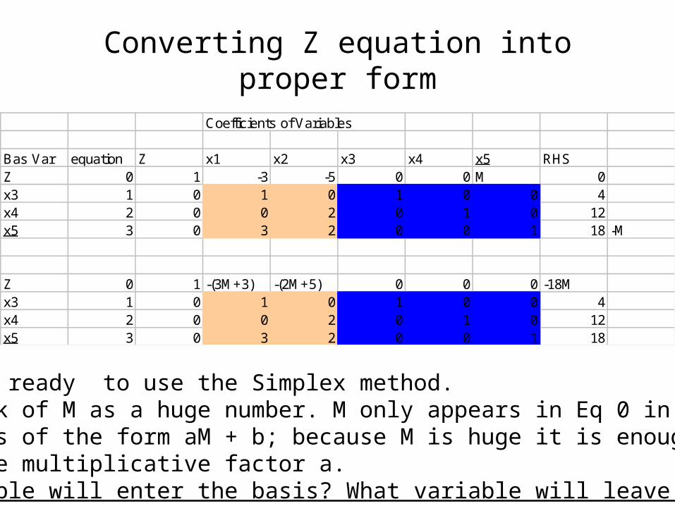
Converting Z equation into proper form

Coefficients of Variables

Bas Var equation Z x1 x2 x3 x4 x5 RHSZ 0 1 -3 -5 0 0 M 0x3 1 0 1 0 1 0 0 4x4 2 0 0 2 0 1 0 12x5 3 0 3 2 0 0 1 18 -M

Z 0 1 -(3M+3) -(2M+5) 0 0 0 -18Mx3 1 0 1 0 1 0 0 4x4 2 0 0 2 0 1 0 12x5 3 0 3 2 0 0 1 18

Now we are ready to use the Simplex method.Note: Think of M as a huge number. M only appears in Eq 0 inExpressions of the form aM + b; because M is huge it is enough toCompare the multiplicative factor a. What variable will enter the basis? What variable will leave the basis?

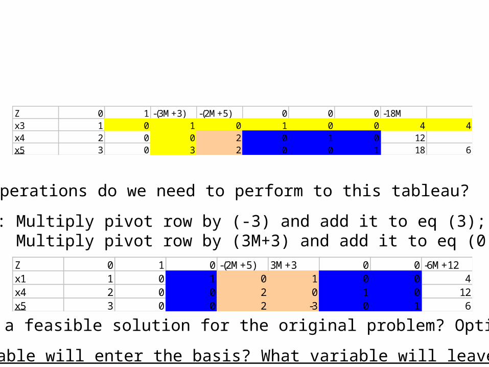
Z 0 1 -(3M+3) -(2M+5) 0 0 0 -18Mx3 1 0 1 0 1 0 0 4 4x4 2 0 0 2 0 1 0 12x5 3 0 3 2 0 0 1 18 6

What operations do we need to perform to this tableau?

Answer: Multiply pivot row by (-3) and add it to eq (3); Multiply pivot row by (3M+3) and add it to eq (0);

What variable will enter the basis? What variable will leave the basis?

Z 0 1 0 -(2M+5) 3M+3 0 0 -6M+12x1 1 0 1 0 1 0 0 4x4 2 0 0 2 0 1 0 12x5 3 0 0 2 -3 0 1 6

Is this a feasible solution for the original problem? Optimal?Why?

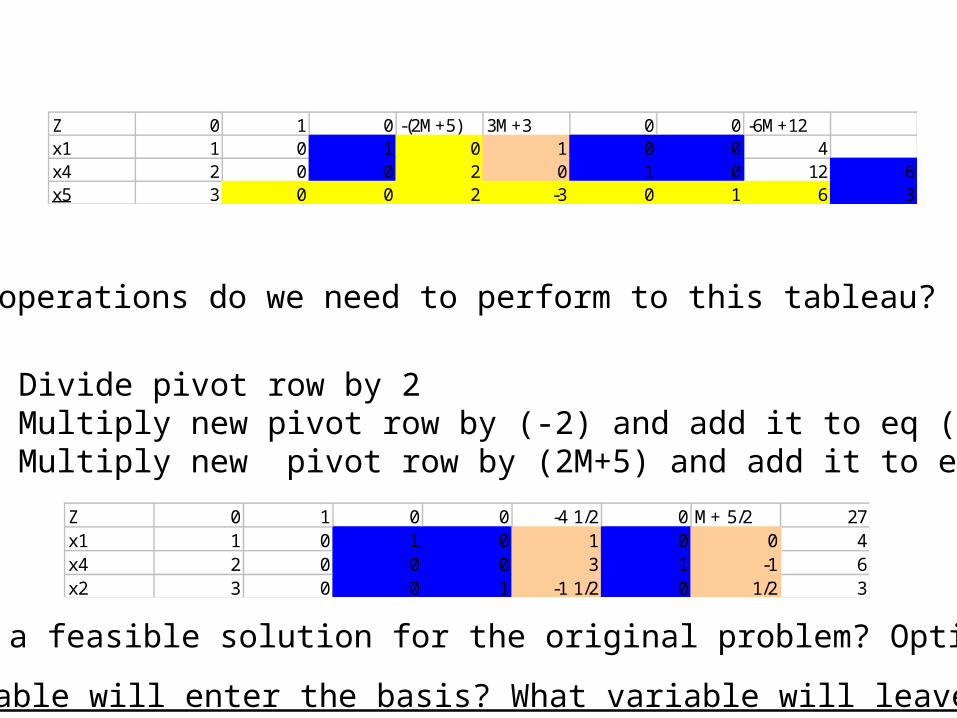
Z 0 1 0 -(2M+5) 3M+3 0 0 -6M+12x1 1 0 1 0 1 0 0 4x4 2 0 0 2 0 1 0 12 6x5 3 0 0 2 -3 0 1 6 3

What operations do we need to perform to this tableau?

Answer: Divide pivot row by 2 Multiply new pivot row by (-2) and add it to eq (2); Multiply new pivot row by (2M+5) and add it to eq (0); Z 0 1 0 0 -4 1/2 0 M+ 5/2 27

x1 1 0 1 0 1 0 0 4x4 2 0 0 0 3 1 -1 6x2 3 0 0 1 -1 1/2 0 1/2 3

Is this a feasible solution for the original problem? Optimal?Why?

What variable will enter the basis? What variable will leave the basis?

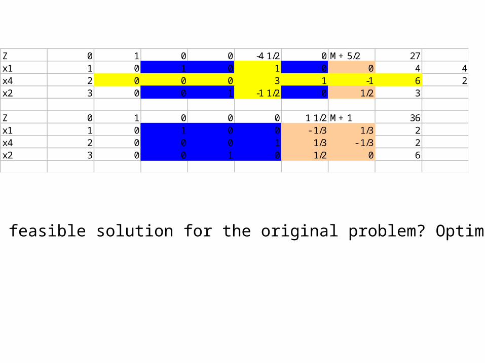
Z 0 1 0 0 -4 1/2 0 M+ 5/2 27x1 1 0 1 0 1 0 0 4 4x4 2 0 0 0 3 1 -1 6 2x2 3 0 0 1 -1 1/2 0 1/2 3

Z 0 1 0 0 0 1 1/2 M+ 1 36x1 1 0 1 0 0 - 1/3 1/3 2x4 2 0 0 0 1 1/3 - 1/3 2x2 3 0 0 1 0 1/2 0 6

Is this a feasible solution for the original problem? Optimal?Why?

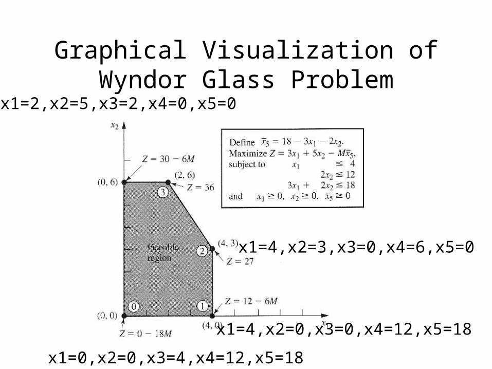
Graphical Visualization of Wyndor Glass Problem

x1=0,x2=0,x3=4,x4=12,x5=18

x1=4,x2=0,x3=0,x4=12,x5=18

x1=4,x2=3,x3=0,x4=6,x5=0

x1=2,x2=5,x3=2,x4=0,x5=0

Handling Negative Right Hand Sides

x1 + x3 <=-1;

-x1 - x3 ≥ 1;

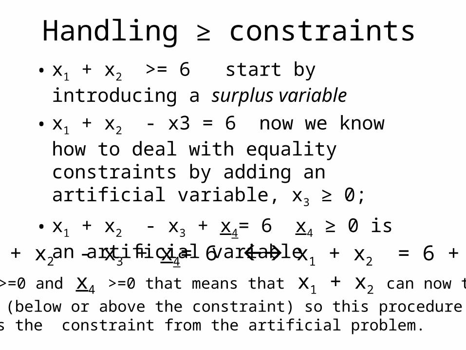
Handling ≥ constraints• x1 + x2 >= 6 start by introducing a surplus

variable

• x1 + x2 - x3 = 6 now we know how to deal with equality constraints by adding an artificial variable, x3 ≥ 0;

• x1 + x2 - x3 + x4= 6 x4 ≥ 0 is an artificial variable

Note: x1 + x2 - x3 + x4= 6 x1 + x2 = 6 + x3 - x4

Since x3 >=0 and x4 >=0 that means that x1 + x2 can now take

any value (below or above the constraint) so this procedure in fact eliminates the constraint from the artificial problem.

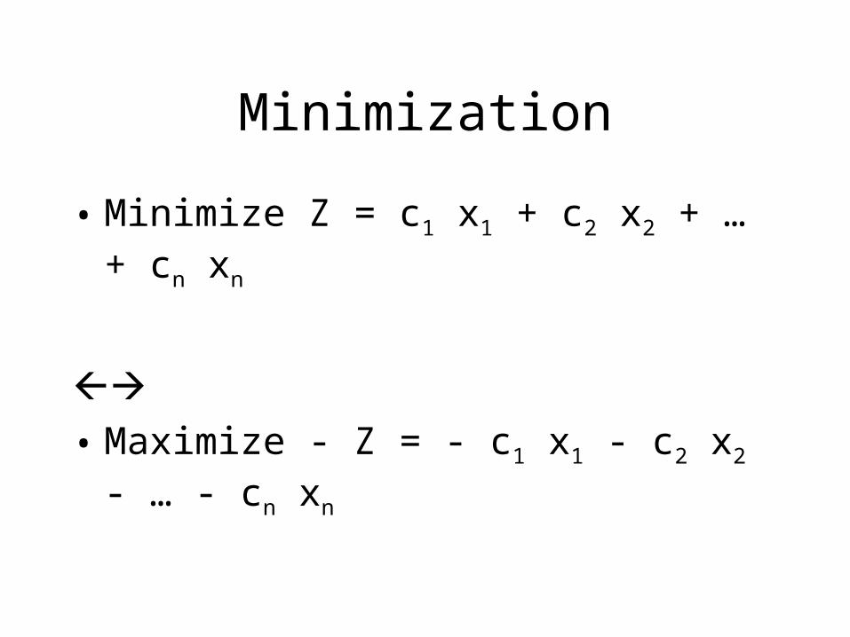
Minimization

• Minimize Z = c1 x1 + c2 x2 + … + cn xn

• Maximize - Z = - c1 x1 - c2 x2 - … - cn xn

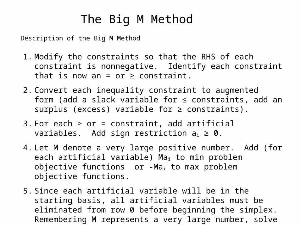
The Big M Method

Description of the Big M Method

1. Modify the constraints so that the RHS of each constraint is nonnegative. Identify each constraint that is now an = or ≥ constraint.

2. Convert each inequality constraint to augmented form (add a slack variable for ≤ constraints, add an surplus (excess) variable for ≥ constraints).

3. For each ≥ or = constraint, add artificial variables. Add sign restriction ai ≥ 0.

4. Let M denote a very large positive number. Add (for each artificial variable) Mai to min problem objective functions or -Mai to max problem objective functions.

5. Since each artificial variable will be in the starting basis, all artificial variables must be eliminated from row 0 before beginning the simplex. Remembering M represents a very large number, solve the transformed problem by the simplex.

Math Programming and Radiation Therapy

Radiation Therapy Overview

• High doses of radiation (energy/unit mass) can kill cells and/or prevent them from growing and dividing

– True for cancer cells and normal cells

• Radiation is attractive because the repair mechanisms for cancer cells is less efficient than for normal cells

(slides adapted from James Orlin’s)

Radiation Therapy Overview• Recent advances in radiation therapy now make it possible

to

– map the cancerous region in greater detail

– aim a larger number of different beamlets with greater specificity

• This has spawned the new field of tomotherapy

• “Optimizing the Delivery of Radiation Therapy to Cancer patients,” by Shepard, Ferris, Olivera, and Mackie, SIAM Review, Vol 41, pp 721-744, 1999.

• Also see http://www.tomotherapy.com/

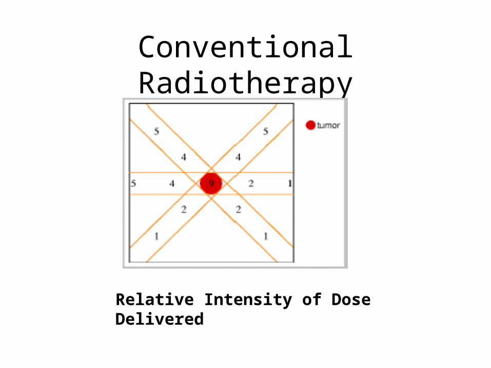
Conventional Radiotherapy

Relative Intensity of Dose Delivered

Conventional Radiotherapy

Relative Intensity of Dose Delivered

Conventional Radiotherapy

• In conventional radiotherapy– 3 to 7 beams of radiation– radiation oncologist and physicist work

together to determine a set of beam angles and beam intensities

– determined by manual “trial-and-error” process

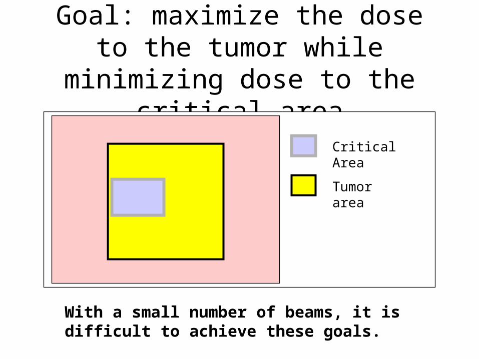
Goal: maximize the dose to the tumor while minimizing dose to the

critical area

Critical Area

Tumor area

With a small number of beams, it is difficult to achieve these goals.

Recent Advances

• More accurate map of tumor area– CT -- Computed Tomography– MRI -- Magnetic Resonance Imaging

• More accurate delivery of radiation– IMRT: Intensity Modulated Radiation Therapy– Tomotherapy

Tomotherapy: a diagram

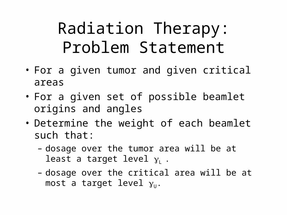
Radiation Therapy: Problem Statement

• For a given tumor and given critical areas• For a given set of possible beamlet origins and

angles• Determine the weight of each beamlet such that:

– dosage over the tumor area will be at least a target level L .

– dosage over the critical area will be at most a target level U.

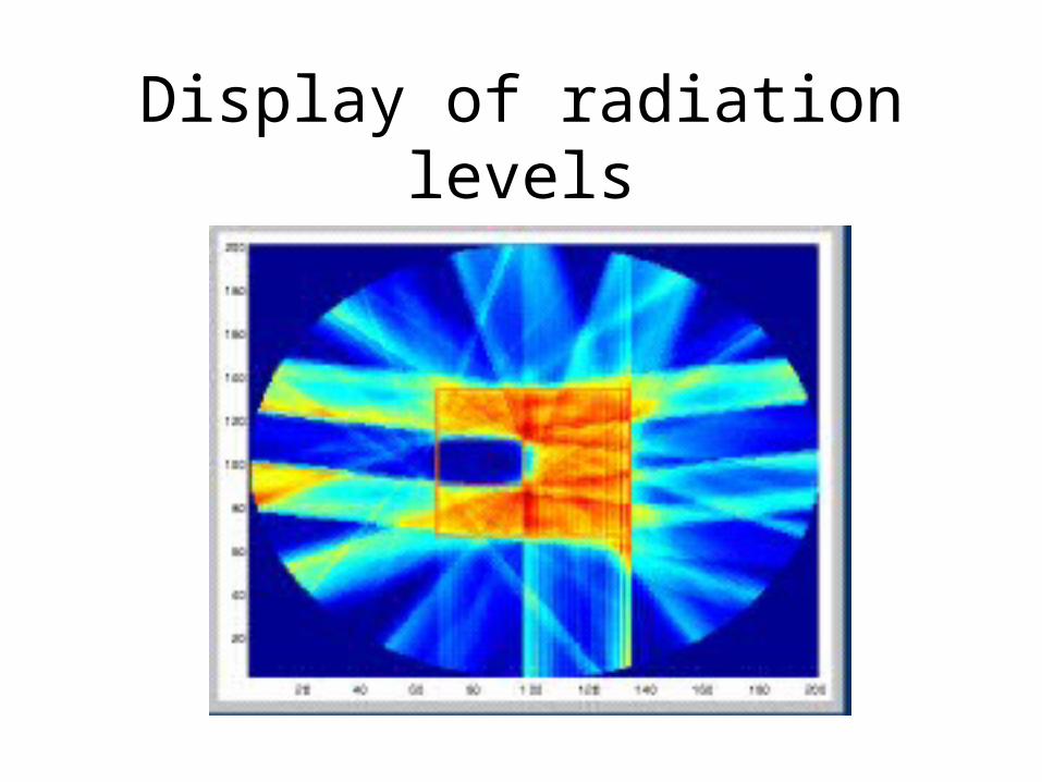
Display of radiation levels

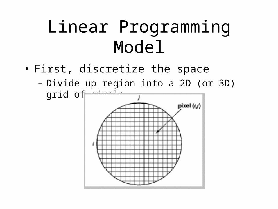
Linear Programming Model

• First, discretize the space– Divide up region into a 2D (or 3D) grid of pixels

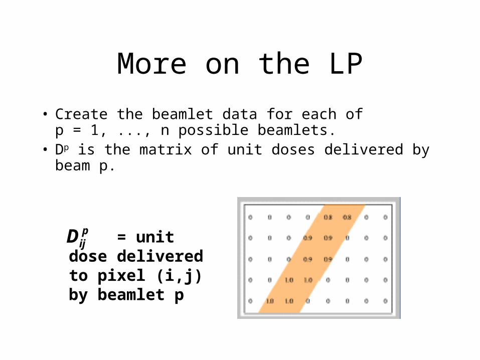
More on the LP

• Create the beamlet data for each of p = 1, ..., n possible beamlets.

• Dp is the matrix of unit doses delivered by beam p.

pijD = unit dose

delivered to pixel (i,j) by beamlet p

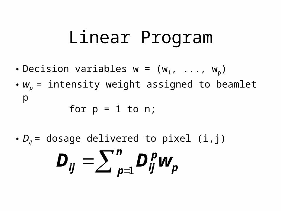
Linear Program

• Decision variables w = (w1, ..., wp)

• wp = intensity weight assigned to beamlet p for p = 1 to n;

• Dij = dosage delivered to pixel (i,j)

1 n p

ij ij ppD D w

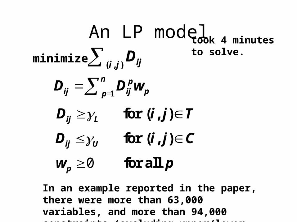
An LP model

1 n p

ij ij ppD D w

minimize ( , ) iji jD

for ( , )ij LD i j T

for ( , )ij UD i j C

0 for allpw p

In an example reported in the paper, there were more than 63,000 variables, and more than 94,000 constraints (excluding upper/lower bounds)

took 4 minutes to solve.

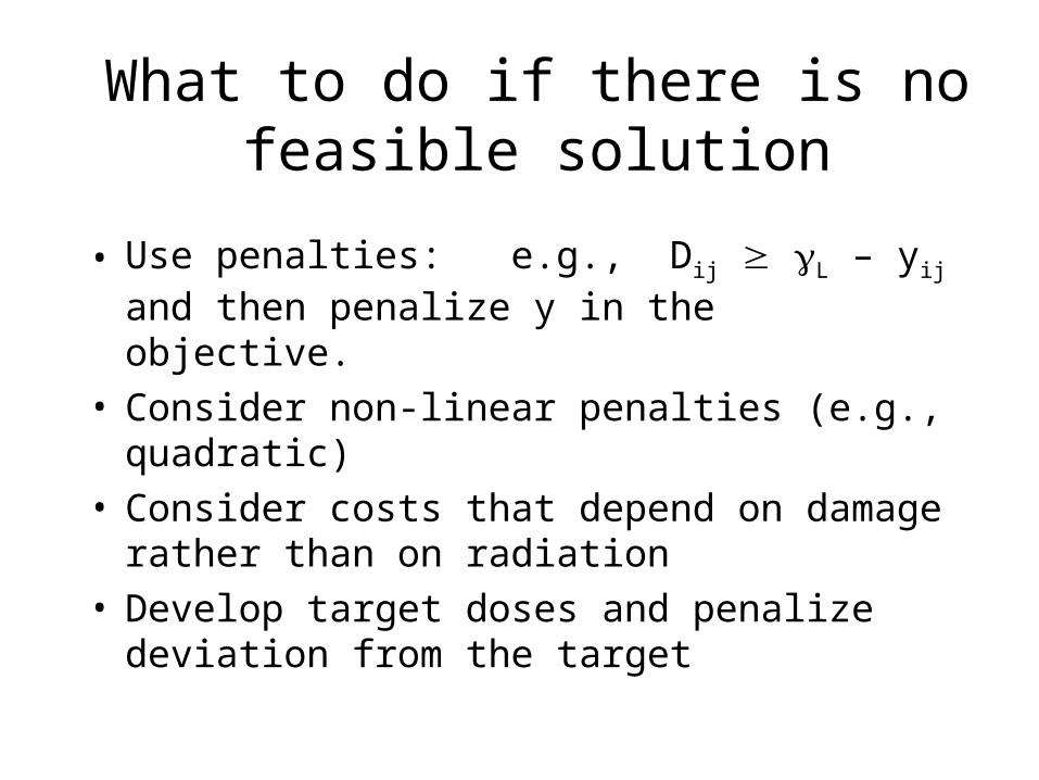
What to do if there is no feasible solution

• Use penalties: e.g., Dij L – yij

and then penalize y in the objective.• Consider non-linear penalties (e.g., quadratic)• Consider costs that depend on damage rather than

on radiation• Develop target doses and penalize deviation from

the target

Optimal Solution for the LP

An Optimal Solution to an NLP

Further considerations

• Minimize damage to critical tissue

• Maximize damage to tumor cells

• Minimize time to carry out the dosage

• LP depends on the technology

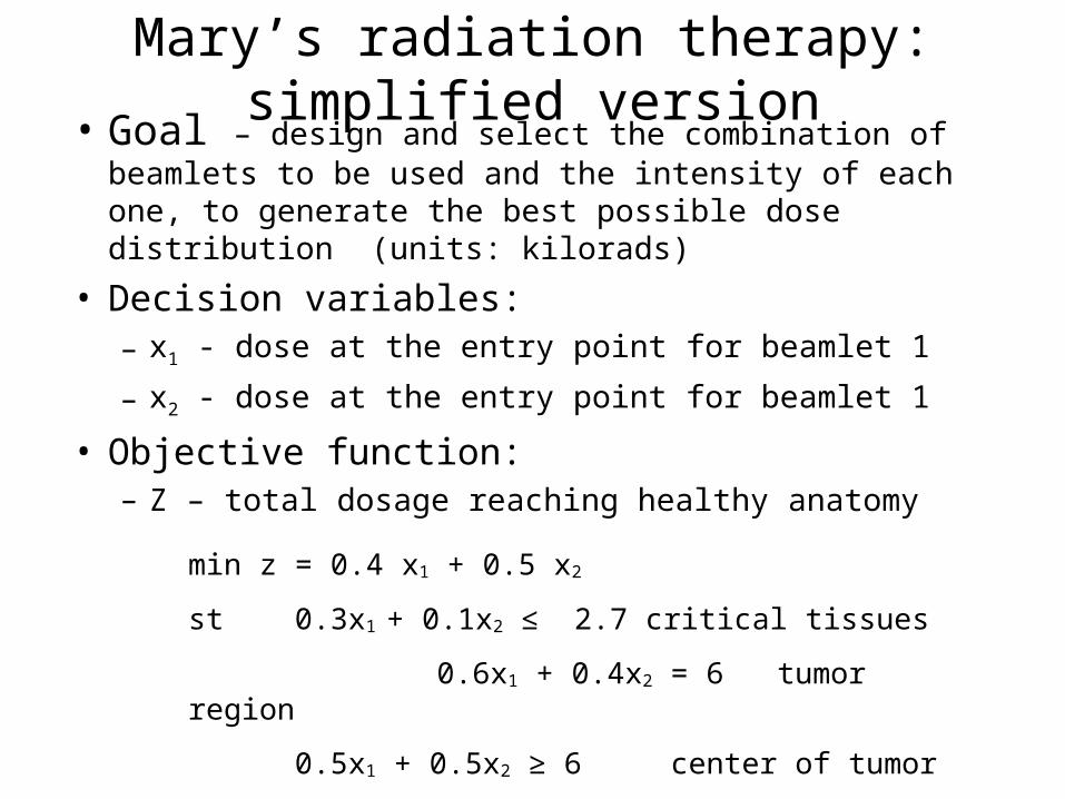
Mary’s radiation therapy: simplified version• Goal – design and select the combination of beamlets to

be used and the intensity of each one, to generate the best possible dose distribution (units: kilorads)

• Decision variables:– x1 - dose at the entry point for beamlet 1

– x2 - dose at the entry point for beamlet 1

• Objective function:– Z – total dosage reaching healthy anatomy

min z = 0.4 x1 + 0.5 x2

st 0.3x1 + 0.1x2 ≤ 2.7 critical tissues

0.6x1 + 0.4x2 = 6 tumor region

0.5x1 + 0.5x2 ≥ 6 center of tumor

x1, x2, > 0

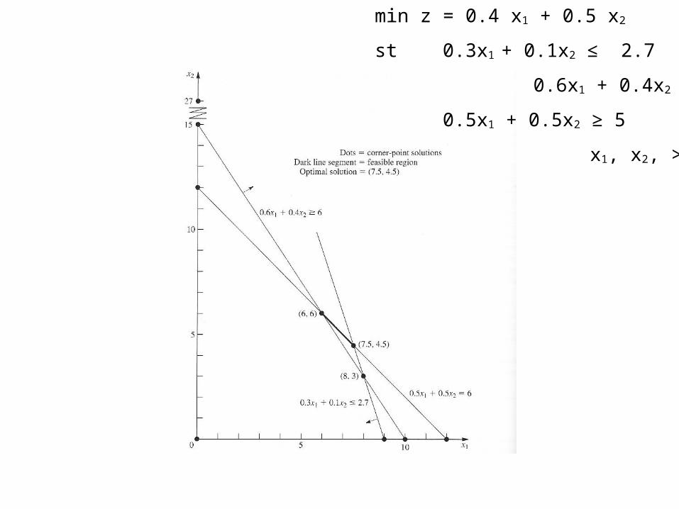
min z = 0.4 x1 + 0.5 x2

st 0.3x1 + 0.1x2 ≤ 2.7

0.6x1 + 0.4x2 = 6

0.5x1 + 0.5x2 ≥ 5

x1, x2, > 0

Getting the problem into augmented form (canonical form) for simplex

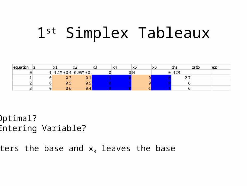
1st Simplex Tableaux

Optimal?Entering Variable?

x1 enters the base and x3 leaves the base

equation z x1 x2 x3 x4 x5 x6 rhs ratio ero0 -1 -1.1M+0.4 -0.95M+0.5 0 0 M 0 -12M1 0 0.3 0.1 1 0 0 0 2.72 0 0.5 0.5 0 1 0 0 63 0 0.6 0.4 0 0 -1 1 6

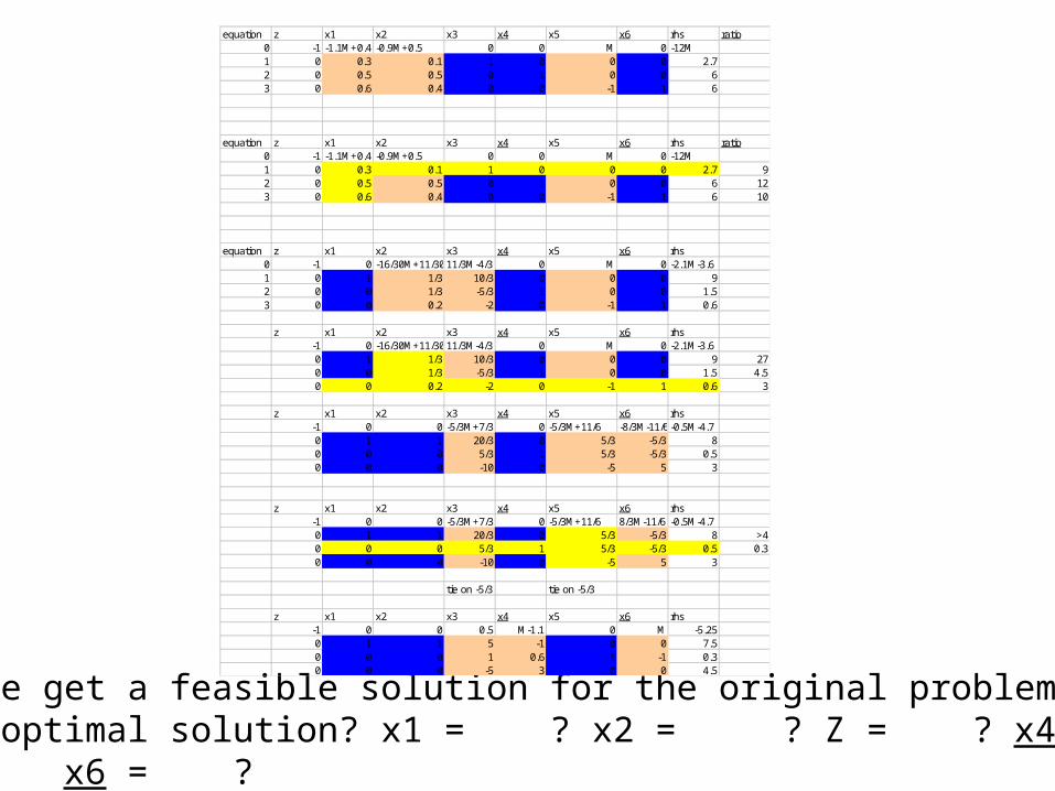
When do we get a feasible solution for the original problem?What the optimal solution? x1 = ? x2 = ? Z = ? x4 = ?x5 = ? x6 = ?

equation z x1 x2 x3 x4 x5 x6 rhs ratio0 -1 -1.1M+0.4 -0.9M+0.5 0 0 M 0 -12M1 0 0.3 0.1 1 0 0 0 2.72 0 0.5 0.5 0 1 0 0 63 0 0.6 0.4 0 0 -1 1 6

equation z x1 x2 x3 x4 x5 x6 rhs ratio0 -1 -1.1M+0.4 -0.9M+0.5 0 0 M 0 -12M1 0 0.3 0.1 1 0 0 0 2.7 92 0 0.5 0.5 0 1 0 0 6 123 0 0.6 0.4 0 0 -1 1 6 10

equation z x1 x2 x3 x4 x5 x6 rhs0 -1 0 -16/30M+11/3011/3M-4/3 0 M 0 -2.1M-3.61 0 1 1/3 10/3 0 0 0 92 0 0 1/3 -5/3 1 0 0 1.53 0 0 0.2 -2 0 -1 1 0.6

z x1 x2 x3 x4 x5 x6 rhs-1 0 -16/30M+11/3011/3M-4/3 0 M 0 -2.1M-3.60 1 1/3 10/3 0 0 0 9 270 0 1/3 -5/3 1 0 0 1.5 4.50 0 0.2 -2 0 -1 1 0.6 3

z x1 x2 x3 x4 x5 x6 rhs-1 0 0 -5/3M+7/3 0 -5/3M+11/6 -8/3M-11/6 -0.5M-4.70 1 1 20/3 0 5/3 -5/3 80 0 0 5/3 1 5/3 -5/3 0.50 0 0 -10 0 -5 5 3

z x1 x2 x3 x4 x5 x6 rhs-1 0 0 -5/3M+7/3 0 -5/3M+11/6 8/3M-11/6 -0.5M-4.70 1 1 20/3 0 5/3 -5/3 8 >40 0 0 5/3 1 5/3 -5/3 0.5 0.30 0 0 -10 0 -5 5 3

tie on -5/3 tie on -5/3

z x1 x2 x3 x4 x5 x6 rhs-1 0 0 0.5 M-1.1 0 M -5.250 1 1 5 -1 0 0 7.50 0 0 1 0.6 1 -1 0.30 0 0 -5 3 0 0 4.5

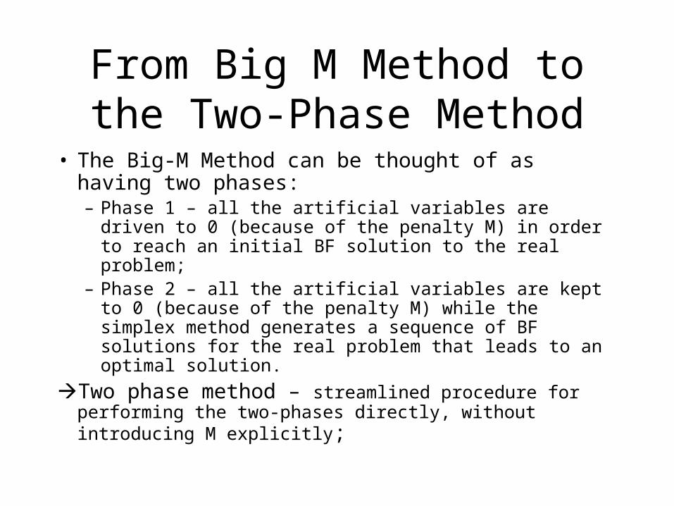
From Big M Method to the Two-Phase Method

• The Big-M Method can be thought of as having two phases:– Phase 1 – all the artificial variables are driven to 0 (because

of the penalty M) in order to reach an initial BF solution to the real problem;

– Phase 2 – all the artificial variables are kept to 0 (because of the penalty M) while the simplex method generates a sequence of BF solutions for the real problem that leads to an optimal solution.

Two phase method – streamlined procedure for performing the two-phases directly, without introducing M explicitly;

Two Phase Method: Mary’s radiation therapy

• Real problem’s objective function: min z = 0.4 x1 + 0.5 x2

• Big M method’s objective function: min z = 0.4 x1 + 0.5 x2 + M x4 + M x6

• Since the two first coefficients are negligible compared to M, the two phase method drops M by using the following objective functions:– Phase 1: minimize z = x4 + x6 (until x4 = , x6 =0)

– Phase 2: min z = 0.4 x1 + 0.5 x2 (with x4 = , x6 =0)

min z = x4 + x6

st

0.3x1 + 0.1x2 + x3 = 2.7

0.6x1 + 0.4x2 + x4 = 6

0.5x1 + 0.5x2 - x5 + x6 = 6

x1, x2, x3, x4 , x5, x6 >= 0

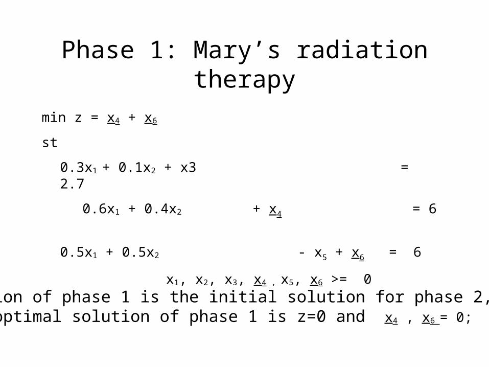
The solution of phase 1 is the initial solution for phase 2, assumingThat the optimal solution of phase 1 is z=0 and x4 , x6 = 0;

Phase 1: Mary’s radiation therapy

min z = 0.4x1 + 0.5x2

st

0.3x1 + 0.1x2 + x3 = 2.7

0.6x1 + 0.4x2 = 6

0.5x1 + 0.5x2 - x5 = 6

x1, x2, x3, x5 >= 0

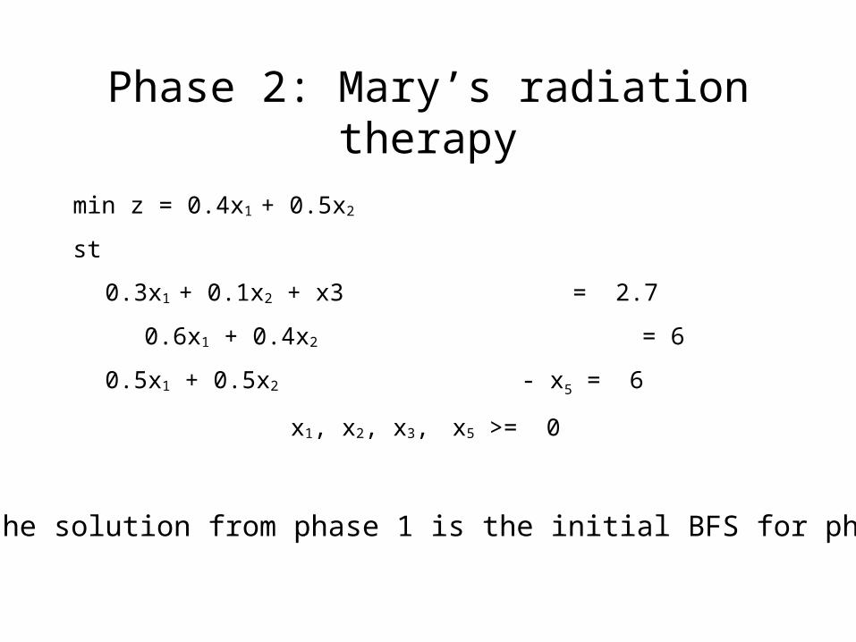
Phase 2: Mary’s radiation therapy

Note: the solution from phase 1 is the initial BFS for phase 2.

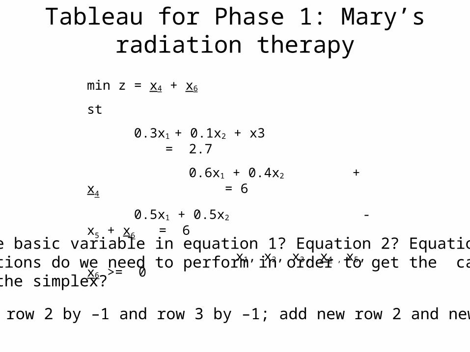
Tableau for Phase 1: Mary’s radiation therapy

min z = x4 + x6

st

0.3x1 + 0.1x2 + x3 = 2.7

0.6x1 + 0.4x2 + x4 = 6

0.5x1 + 0.5x2 - x5 + x6 = 6

x1, x2, x3, x4 , x5, x6 >= 0

What is the basic variable in equation 1? Equation 2? Equation 3?What operations do we need to perform in order to get the canonical form for the simplex?

(multiply row 2 by –1 and row 3 by –1; add new row 2 and new row 3 to row 0)

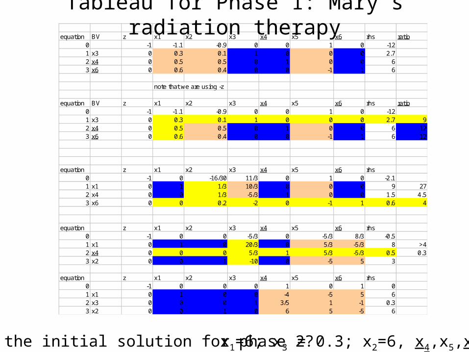
equation BV z x1 x2 x3 x4 x5 x6 rhs ratio0 -1 -1.1 -0.9 0 0 1 0 -121 x3 0 0.3 0.1 1 0 0 0 2.72 x4 0 0.5 0.5 0 1 0 0 63 x6 0 0.6 0.4 0 0 -1 1 6

note that we are using -z

equation BV z x1 x2 x3 x4 x5 x6 rhs ratio0 -1 -1.1 -0.9 0 0 1 0 -121 x3 0 0.3 0.1 1 0 0 0 2.7 92 x4 0 0.5 0.5 0 1 0 0 6 123 x6 0 0.6 0.4 0 0 -1 1 6 12

equation z x1 x2 x3 x4 x5 x6 rhs0 -1 0 -16/30 11/3 0 1 0 -2.11 x1 0 1 1/3 10/3 0 0 0 9 272 x4 0 0 1/3 -5/3 1 0 0 1.5 4.53 x6 0 0 0.2 -2 0 -1 1 0.6 4

equation z x1 x2 x3 x4 x5 x6 rhs0 -1 0 0 -5/3 0 -5/3 8/3 -0.51 x1 0 1 0 20/3 0 5/3 -5/3 8 >42 x4 0 0 0 5/3 1 5/3 -5/3 0.5 0.33 x2 0 0 1 -10 0 -5 5 3

equation z x1 x2 x3 x4 x5 x6 rhs0 -1 0 0 0 1 0 1 01 x1 0 1 0 0 -4 -5 5 62 x3 0 0 0 1 3/5 1 -1 0.33 x2 0 0 1 0 6 5 -5 6

Tableau for Phase 1: Mary’s radiation therapy

What’s the initial solution for phase 2? x1=6; x3 = 0.3; x2=6, x4,x5,x6=0

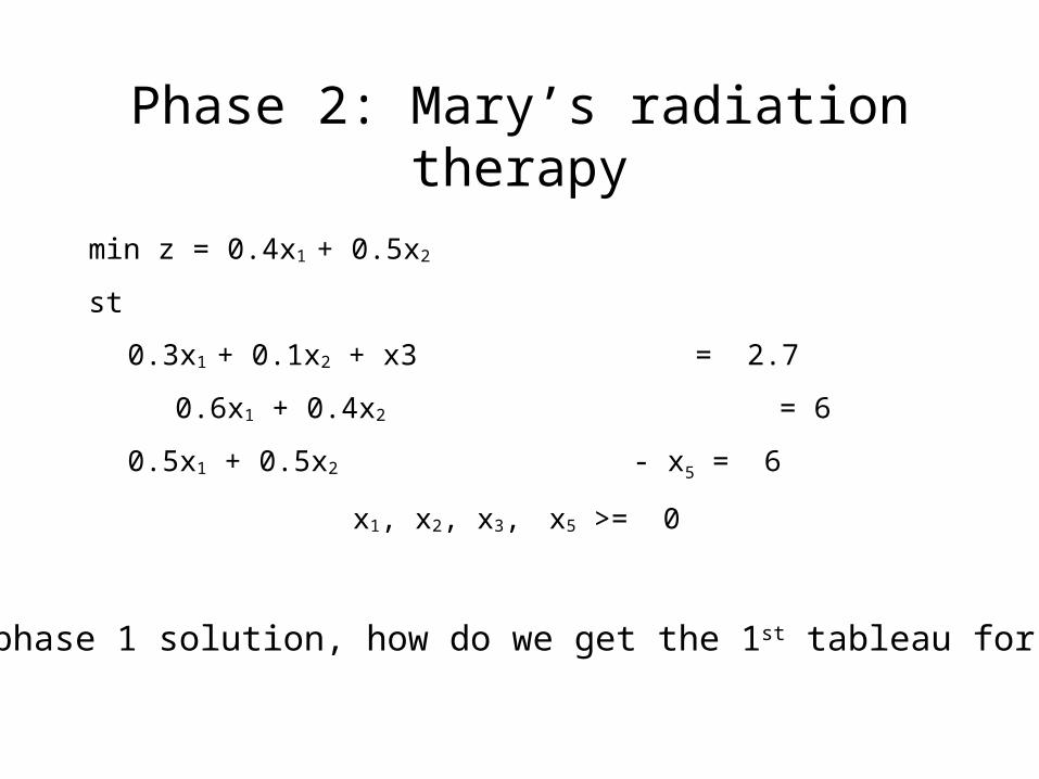
min z = 0.4x1 + 0.5x2

st

0.3x1 + 0.1x2 + x3 = 2.7

0.6x1 + 0.4x2 = 6

0.5x1 + 0.5x2 - x5 = 6

x1, x2, x3, x5 >= 0

Phase 2: Mary’s radiation therapy

Using phase 1 solution, how do we get the 1st tableau for phase 2?

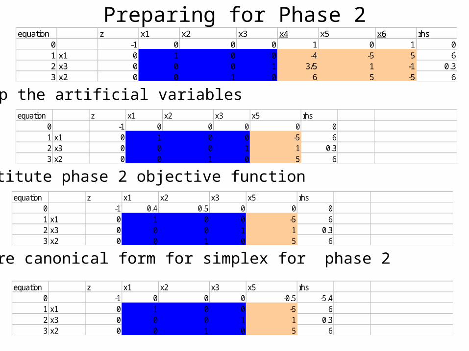
Preparing for Phase 2equation z x1 x2 x3 x4 x5 x6 rhs

0 -1 0 0 0 1 0 1 01 x1 0 1 0 0 -4 -5 5 62 x3 0 0 0 1 3/5 1 -1 0.33 x2 0 0 1 0 6 5 -5 6

equation z x1 x2 x3 x5 rhs0 -1 0 0 0 0 01 x1 0 1 0 0 -5 62 x3 0 0 0 1 1 0.33 x2 0 0 1 0 5 6

Drop the artificial variables

Substitute phase 2 objective functionequation z x1 x2 x3 x5 rhs

0 -1 0.4 0.5 0 0 01 x1 0 1 0 0 -5 62 x3 0 0 0 1 1 0.33 x2 0 0 1 0 5 6

equation z x1 x2 x3 x5 rhs0 -1 0 0 0 -0.5 -5.41 x1 0 1 0 0 -5 62 x3 0 0 0 1 1 0.33 x2 0 0 1 0 5 6

Restore canonical form for simplex for phase 2

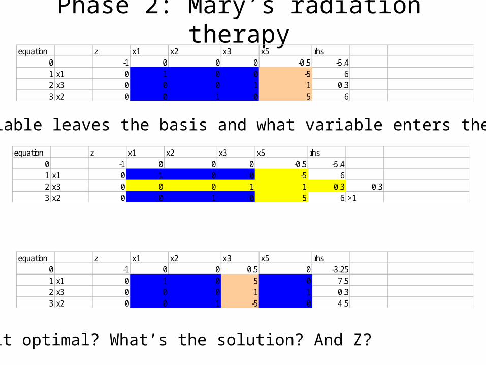
Phase 2: Mary’s radiation therapyequation z x1 x2 x3 x5 rhs

0 -1 0 0 0 -0.5 -5.41 x1 0 1 0 0 -5 62 x3 0 0 0 1 1 0.33 x2 0 0 1 0 5 6

equation z x1 x2 x3 x5 rhs0 -1 0 0 0 -0.5 -5.41 x1 0 1 0 0 -5 62 x3 0 0 0 1 1 0.3 0.33 x2 0 0 1 0 5 6 >1

What variable leaves the basis and what variable enters the basis?

equation z x1 x2 x3 x5 rhs0 -1 0 0 0.5 0 -3.251 x1 0 1 0 5 0 7.52 x3 0 0 0 1 1 0.33 x2 0 0 1 -5 0 4.5

Is it optimal? What’s the solution? And Z?

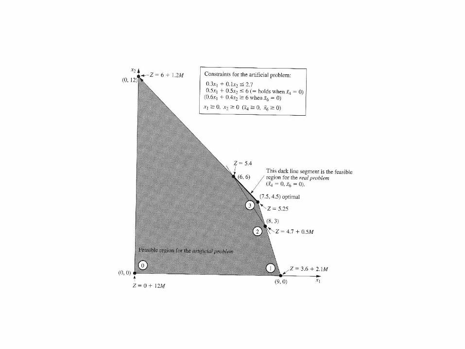
Graphical Visualization of Phase I and Phase II

Big M Method vs. Two-phase Method

The two-phase method streamlines the Big M method by using only the multiplicative factors in phase 1 and by dropping the artificial variables in phase 2.

Two-phase method is commonly used in computational implementations.

No Feasible Solutions

• If the original problem has no feasible solutions, then either the Big M method or the phase 1 of the two-phase method yields a final solution that has at least one artificial variable greater than zero.

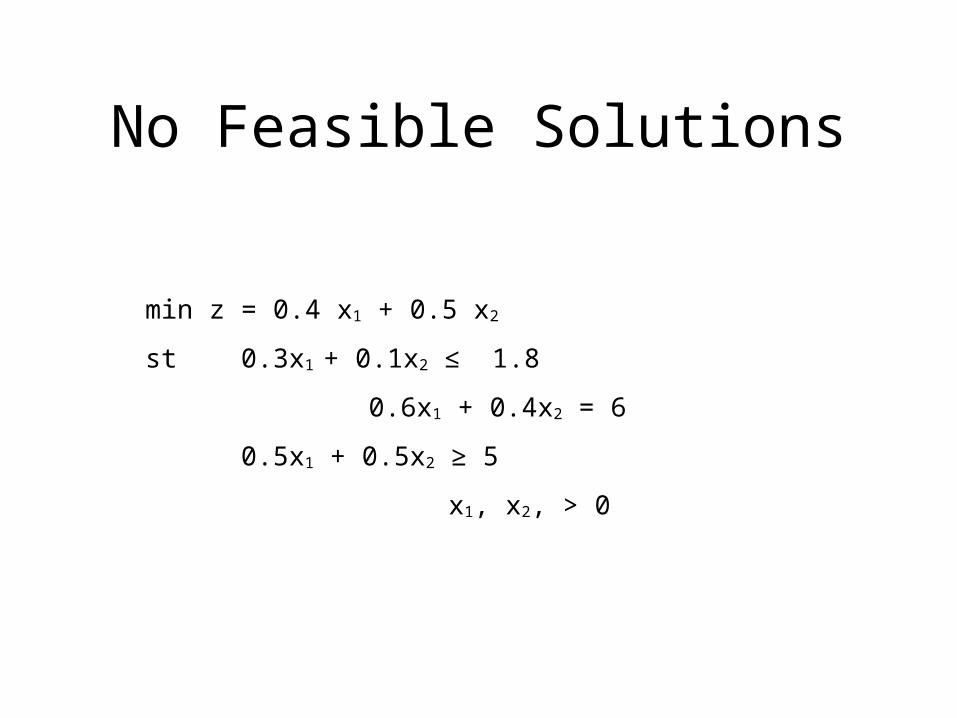
No Feasible Solutions

min z = 0.4 x1 + 0.5 x2

st 0.3x1 + 0.1x2 ≤ 1.8

0.6x1 + 0.4x2 = 6

0.5x1 + 0.5x2 ≥ 5

x1, x2, > 0

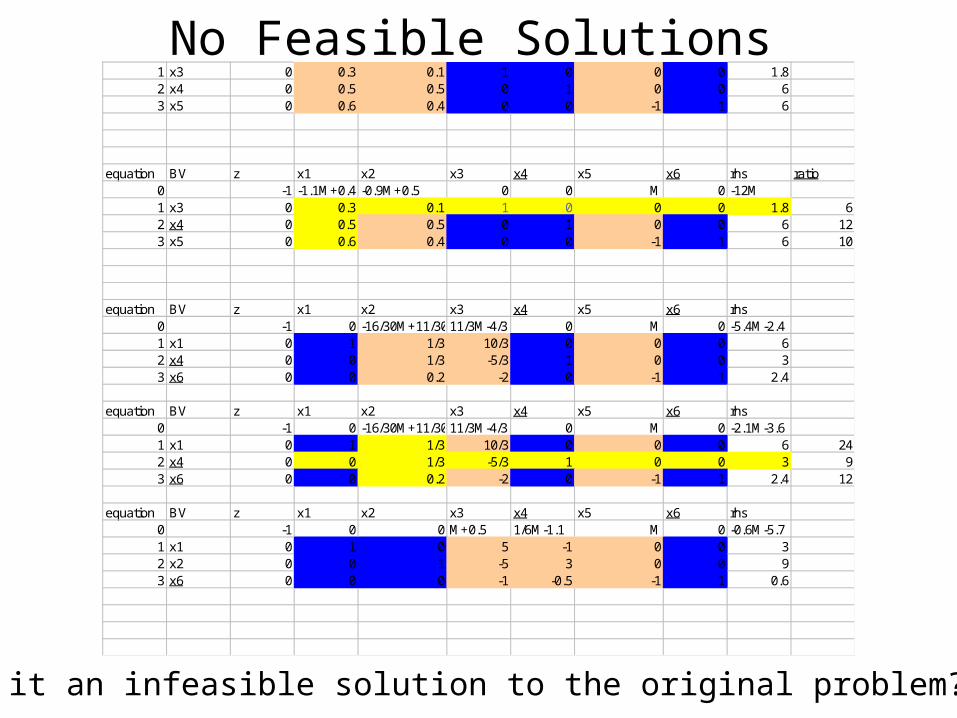
No Feasible Solutions1 x3 0 0.3 0.1 1 0 0 0 1.82 x4 0 0.5 0.5 0 1 0 0 63 x5 0 0.6 0.4 0 0 -1 1 6

equation BV z x1 x2 x3 x4 x5 x6 rhs ratio0 -1 -1.1M+0.4 -0.9M+0.5 0 0 M 0 -12M1 x3 0 0.3 0.1 1 0 0 0 1.8 62 x4 0 0.5 0.5 0 1 0 0 6 123 x5 0 0.6 0.4 0 0 -1 1 6 10

equation BV z x1 x2 x3 x4 x5 x6 rhs0 -1 0 -16/30M+11/3011/3M-4/3 0 M 0 -5.4M-2.41 x1 0 1 1/3 10/3 0 0 0 62 x4 0 0 1/3 -5/3 1 0 0 33 x6 0 0 0.2 -2 0 -1 1 2.4

equation BV z x1 x2 x3 x4 x5 x6 rhs0 -1 0 -16/30M+11/3011/3M-4/3 0 M 0 -2.1M-3.61 x1 0 1 1/3 10/3 0 0 0 6 242 x4 0 0 1/3 -5/3 1 0 0 3 93 x6 0 0 0.2 -2 0 -1 1 2.4 12

equation BV z x1 x2 x3 x4 x5 x6 rhs0 -1 0 0 M+0.5 1/6M-1.1 M 0 -0.6M-5.71 x1 0 1 0 5 -1 0 0 32 x2 0 0 1 -5 3 0 0 93 x6 0 0 0 -1 -0.5 -1 1 0.6

Why is it an infeasible solution to the original problem?

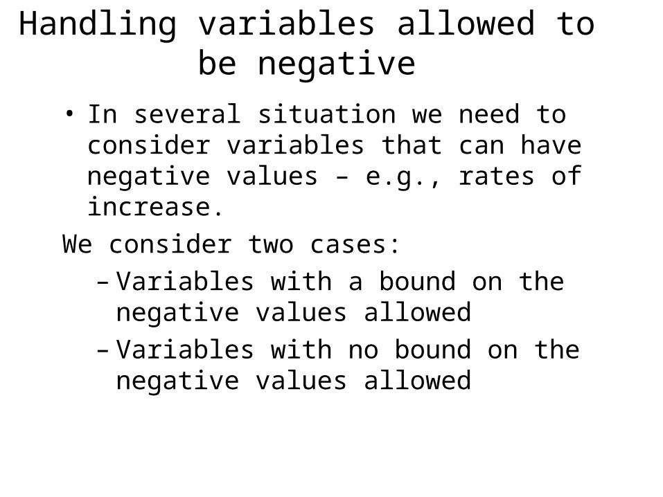
Handling variables allowed to be negative

• In several situation we need to consider variables that can have negative values – e.g., rates of increase.

We consider two cases:– Variables with a bound on the negative values

allowed– Variables with no bound on the negative values

allowed

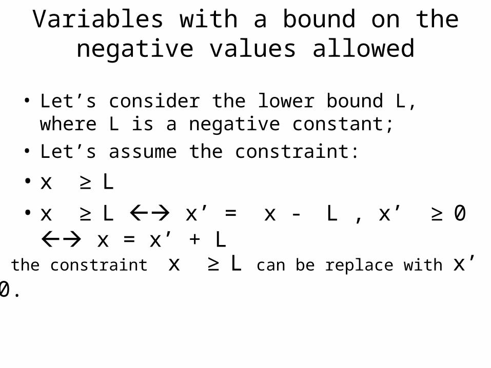
Variables with a bound on the negative values allowed

• Let’s consider the lower bound L, where L is a negative constant;

• Let’s assume the constraint:

• x ≥ L• x ≥ L x’ = x - L , x’ ≥ 0 x = x’ + L

So x and the constraint x ≥ L can be replace with x’ + L and

x’ ≥ 0.

Wyndor Glass

• x1 – rate of increase in production (does not go below –10)

Maximize Z = 3 x1+ 5 x2subject to

x1 ≤ 42x2≤ 123x1 + 2x2 ≤ 18

andx1 ≥ -10, x2 ≥0.

Let x1 = rate of increase of the number of doors to produce

x2 = the number of windows to produce

Maximize Z = 3 (x’-10) + 5 x2subject to

(x’-10) ≤ 42 x2 ≤ 123 (x’-10) + 2x2 ≤ 18

and (x’-10) ≥ -10, x2 ≥ 0.

Maximize Z = -30 + 3x’ + 5 x2subject to

x’≤ 142x’ ≤ 123x’+ 2x2 ≤ 48

and x’ ≥ 0, x2 ≥ 0.

Note: A similar technique can be used when L is positive and a variableis subject to the constraint: x ≥ L

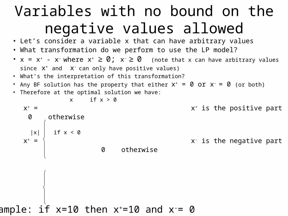
Variables with no bound on the negative values allowed

• Let’s consider a variable x that can have arbitrary values• What transformation do we perform to use the LP model?• x = x+ - x- where x+ ≥ 0; x- ≥ 0 (note that x can have arbitrary values since x+ and x- can

only have positive values)• What’s the interpretation of this transformation? • Any BF solution has the property that either x+ = 0 or x- = 0 (or both)• Therefore at the optimal solution we have: x if x > 0

x+ = x+ is the positive part 0 otherwise

|x| if x < 0

x+ = x- is the negative part 0 otherwise

Example: if x=10 then x+=10 and x-= 0

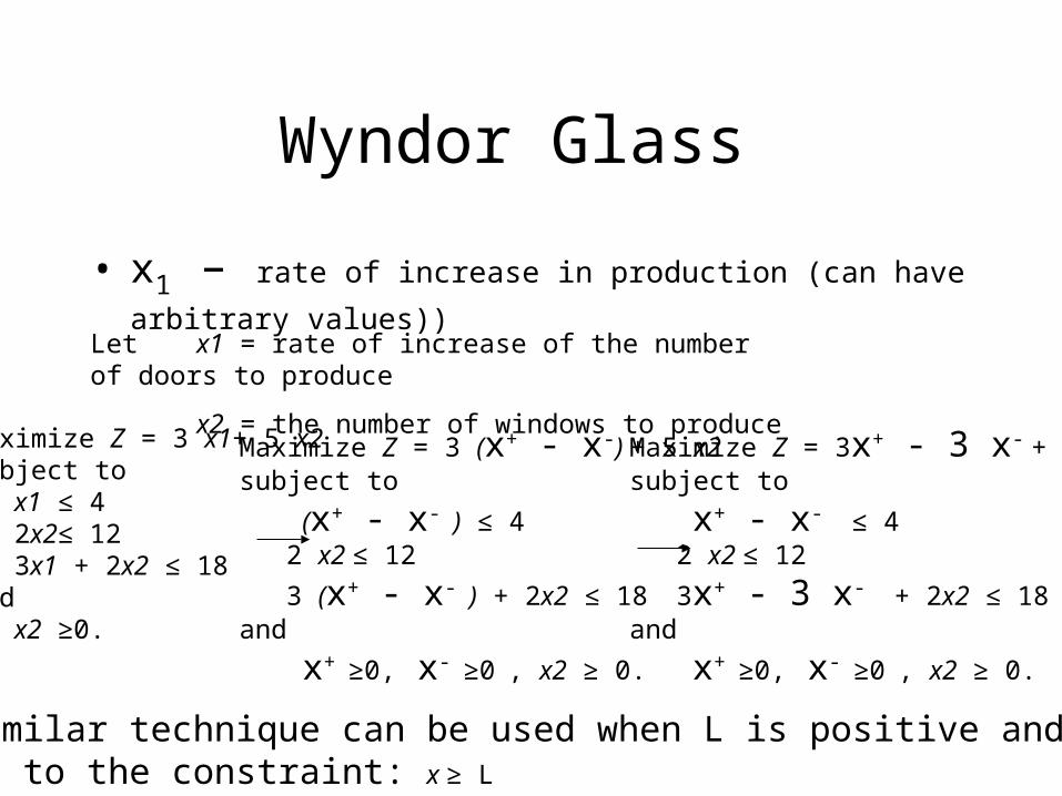
Wyndor Glass

• x1 – rate of increase in production (can have arbitrary values))

Maximize Z = 3 x1+ 5 x2subject to

x1 ≤ 42x2≤ 123x1 + 2x2 ≤ 18

andx2 ≥0.

Let x1 = rate of increase of the number of doors to produce

x2 = the number of windows to produce

Maximize Z = 3 (x+ - x-) + 5 x2subject to

(x+ - x- ) ≤ 42 x2 ≤ 12

3 (x+ - x- ) + 2x2 ≤ 18and

x+ ≥0, x- ≥0 , x2 ≥ 0.

Note: A similar technique can be used when L is positive and a variableis subject to the constraint: x ≥ L

Maximize Z = 3x+ - 3 x- + 5 x2subject to

x+ - x- ≤ 42 x2 ≤ 12

3x+ - 3 x- + 2x2 ≤ 18and

x+ ≥0, x- ≥0 , x2 ≥ 0.

• From a computational view point this approach has the disadvantage of introducing new variables. If all the variables can have arbitrary values the transformed model will have twice as many variables. Can we do better?

• Yes – by introducing only one additional variable. All variables xj are replaced by:– with xj = xj’-x’’ where xj’ ≥0, x’’ ≥ 0 (x’’ is the same for all

variables; -x’’ corresponds to the largest (in absolute terms) negative

original variable; xj’is the amount by which xj exceeds x’’.)