computational methods for nanoscale bio sensors
TRANSCRIPT
Computational Methods for Nanoscale
Bio-Sensors
S. Adhikari1
1Chair of Aerospace Engineering, College of Engineering, Swansea University, Singleton Park, SwanseaSA2 8PP, UK
Fifth Serbian Congress on Theoretical and Applied Mechanics, Belgrade
Adhikari (Swansea) Computational Methods for Nanoscale Bio-Sensors June 15, 2015 1

Swansea University
Adhikari (Swansea) Computational Methods for Nanoscale Bio-Sensors June 15, 2015 2

Swansea University
Adhikari (Swansea) Computational Methods for Nanoscale Bio-Sensors June 15, 2015 3
Outline
1 Introduction
2 One-dimensional sensors - classical approach
Static deformation approximationDynamic mode approximation
3 One-dimensional sensors - nonlocal approach
Attached biomolecules as point massAttached biomolecules as distributed mass
4 Two-dimensional sensors - classical approach
5 Two-dimensional sensors - nonlocal approach
6 Conclusions
Adhikari (Swansea) Computational Methods for Nanoscale Bio-Sensors June 15, 2015 4
Introduction
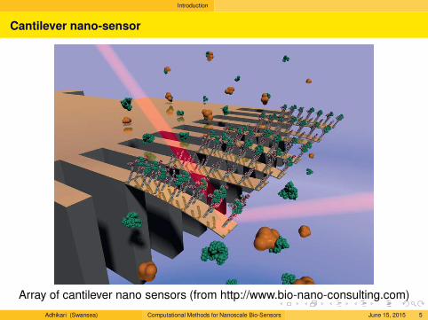
Cantilever nano-sensor
Array of cantilever nano sensors (from http://www.bio-nano-consulting.com)
Adhikari (Swansea) Computational Methods for Nanoscale Bio-Sensors June 15, 2015 5
Introduction
Mass sensing - an inverse problem
This talk will focus on the detection of mass based on shift in frequency.
Mass sensing is an inverse problem.
The “answer” in general in non-unique. An added mass at a certain pointon the sensor will produce an unique frequency shift. However, for agiven frequency shift, there can be many possible combinations of massvalues and locations.
Therefore, predicting the frequency shift - the so called “forward problem”is not enough for sensor development.
Advanced modelling and computation methods are available for theforward problem. However, they may not be always readily suitable for theinverse problem if the formulation is “complex” to start with.
Often, a carefully formulated simplified computational approach could bemore suitable for the inverse problem and consequently for reliablesensing.
Adhikari (Swansea) Computational Methods for Nanoscale Bio-Sensors June 15, 2015 6

Introduction
The need for “instant” calculation
Sensing calculations must be performed very quickly - almost in real time withvery little computational power (fast and cheap devices).
Adhikari (Swansea) Computational Methods for Nanoscale Bio-Sensors June 15, 2015 7
One-dimensional sensors - classical approach Static deformation approximation
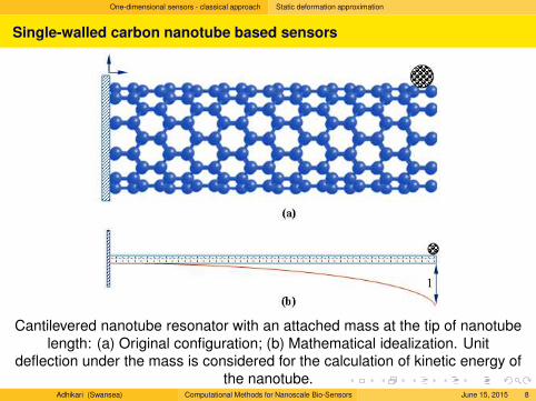
Single-walled carbon nanotube based sensors
Cantilevered nanotube resonator with an attached mass at the tip of nanotubelength: (a) Original configuration; (b) Mathematical idealization. Unit
deflection under the mass is considered for the calculation of kinetic energy ofthe nanotube.
Adhikari (Swansea) Computational Methods for Nanoscale Bio-Sensors June 15, 2015 8
One-dimensional sensors - classical approach Static deformation approximation
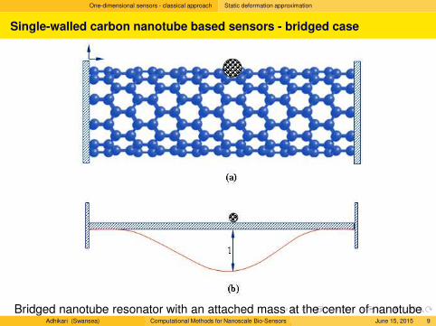
Single-walled carbon nanotube based sensors - bridged case
Bridged nanotube resonator with an attached mass at the center of nanotubelength: (a) Original configuration; (b) Mathematical idealization. UnitAdhikari (Swansea) Computational Methods for Nanoscale Bio-Sensors June 15, 2015 9
One-dimensional sensors - classical approach Static deformation approximation
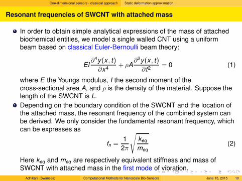
Resonant frequencies of SWCNT with attached mass
In order to obtain simple analytical expressions of the mass of attachedbiochemical entities, we model a single walled CNT using a uniformbeam based on classical Euler-Bernoulli beam theory:
EI∂4y(x , t)
∂x4+ ρA
∂2y(x , t)
∂t2= 0 (1)
where E the Youngs modulus, I the second moment of thecross-sectional area A, and ρ is the density of the material. Suppose thelength of the SWCNT is L.
Depending on the boundary condition of the SWCNT and the location ofthe attached mass, the resonant frequency of the combined system canbe derived. We only consider the fundamental resonant frequency, whichcan be expresses as
fn =1
2π
√
keq
meq(2)
Here keq and meq are respectively equivalent stiffness and mass ofSWCNT with attached mass in the first mode of vibration.
Adhikari (Swansea) Computational Methods for Nanoscale Bio-Sensors June 15, 2015 10
One-dimensional sensors - classical approach Static deformation approximation
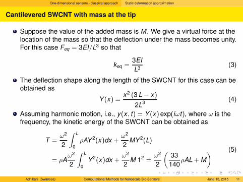
Cantilevered SWCNT with mass at the tip
Suppose the value of the added mass is M. We give a virtual force at thelocation of the mass so that the deflection under the mass becomes unity.For this case Feq = 3EI/L3 so that
keq =3EI
L3(3)
The deflection shape along the length of the SWCNT for this case can beobtained as
Y (x) =x2 (3 L − x)
2L3
(4)
Assuming harmonic motion, i.e., y(x , t) = Y (x)exp(iωt), where ω is thefrequency, the kinetic energy of the SWCNT can be obtained as
T =ω2
2
∫ L
0
ρAY 2(x)dx +ω2
2MY 2(L)
= ρAω2
2
∫ L
0
Y 2(x)dx +ω2
2M 12 =
ω2
2
(33
140ρAL + M
) (5)
Adhikari (Swansea) Computational Methods for Nanoscale Bio-Sensors June 15, 2015 11
One-dimensional sensors - classical approach Static deformation approximation
Cantilevered SWCNT with mass at the tip
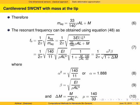
Therefore
meq =33
140ρAL + M (6)
The resonant frequency can be obtained using equation (48) as
fn =1
2π
√
keq
meq=
1
2π
√
3EI/L3
33140
ρAL + M
=1
2π
√
140
11
√
EI
ρAL4
√
1
1 + MρAL
14033
=1
2π
α2β√1 +∆M
(7)
where
α2 =
√
140
11or α = 1.888 (8)
β =
√
EI
ρAL4(9)
and ∆M =M
ρALµ, µ =
140
33(10)
Adhikari (Swansea) Computational Methods for Nanoscale Bio-Sensors June 15, 2015 12
One-dimensional sensors - classical approach Static deformation approximation
Cantilevered SWCNT with mass at the tip
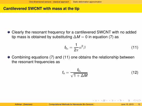
Clearly the resonant frequency for a cantilevered SWCNT with no addedtip mass is obtained by substituting ∆M = 0 in equation (7) as
f0n=
1
2πα2β (11)
Combining equations (7) and (11) one obtains the relationship betweenthe resonant frequencies as
fn =f0n√
1 +∆M(12)
Adhikari (Swansea) Computational Methods for Nanoscale Bio-Sensors June 15, 2015 13
One-dimensional sensors - classical approach Static deformation approximation
General derivation of the sensor equations
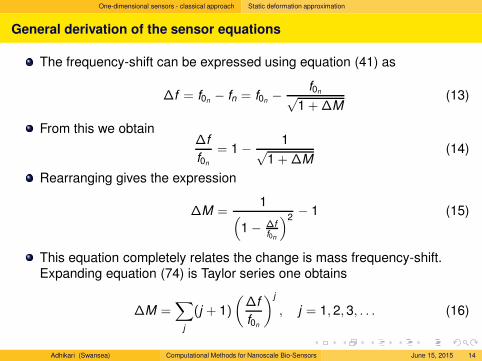
The frequency-shift can be expressed using equation (41) as
∆f = f0n− fn = f0n
− f0n√1 +∆M
(13)
From this we obtain∆f
f0n
= 1 − 1√1 +∆M
(14)
Rearranging gives the expression
∆M =1
(
1 − ∆ff0n
)2− 1 (15)
This equation completely relates the change is mass frequency-shift.Expanding equation (74) is Taylor series one obtains
∆M =∑
j
(j + 1)
(∆f
f0n
)j
, j = 1, 2, 3, . . . (16)
Adhikari (Swansea) Computational Methods for Nanoscale Bio-Sensors June 15, 2015 14
One-dimensional sensors - classical approach Static deformation approximation
General derivation of the sensor equations
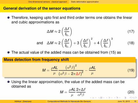
Therefore, keeping upto first and third order terms one obtains the linearand cubic approximations as
∆M ≈ 2
(∆f
f0n
)
(17)
and ∆M ≈ 2
(∆f
f0n
)
+ 3
(∆f
f0n
)2
+ 4
(∆f
f0n
)3
(18)
The actual value of the added mass can be obtained from (15) as
Mass detection from frequency shift
M =ρAL
µ
(α2β
)2
(α2β − 2π∆f )2− ρAL
µ(19)
Using the linear approximation, the value of the added mass can beobtained as
M =ρAL
µ
2π∆f
α2β(20)
Adhikari (Swansea) Computational Methods for Nanoscale Bio-Sensors June 15, 2015 15
One-dimensional sensors - classical approach Static deformation approximation
General derivation of the sensor equations
10−2
10−1
100
10−2
10−1
100
101
102
103
104
Frequency shift: ∆f 2π/α2β
Cha
nge
in m
ass:
M µ/ρ
A L
exact analyticallinear approximationcubic approximation
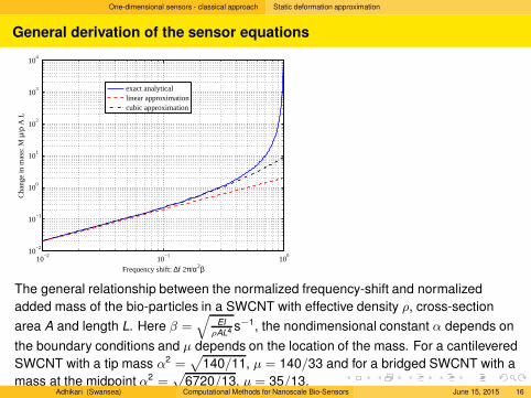
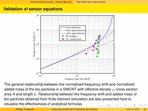
The general relationship between the normalized frequency-shift and normalized
added mass of the bio-particles in a SWCNT with effective density ρ, cross-section
area A and length L. Here β =
√
EI
ρAL4 s−1, the nondimensional constant α depends on
the boundary conditions and µ depends on the location of the mass. For a cantilevered
SWCNT with a tip mass α2=
√
140/11, µ = 140/33 and for a bridged SWCNT with a
mass at the midpoint α2=
√
6720/13, µ = 35/13.Adhikari (Swansea) Computational Methods for Nanoscale Bio-Sensors June 15, 2015 16
One-dimensional sensors - classical approach Static deformation approximation
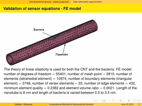
Validation of sensor equations - FE model
The theory of linear elasticity is used for both the CNT and the bacteria. FE model:
number of degrees of freedom = 55401, number of mesh point = 2810, number of
elements (tetrahedral element) = 10974, number of boundary elements (triangular
element) = 3748, number of vertex elements = 22, number of edge elements = 432,
minimum element quality = 0.2382 and element volume ratio = 0.0021. Length of the
nanotube is 8 nm and length of bacteria is varied between 0.5 to 3.5 nm.
Adhikari (Swansea) Computational Methods for Nanoscale Bio-Sensors June 15, 2015 17
One-dimensional sensors - classical approach Static deformation approximation
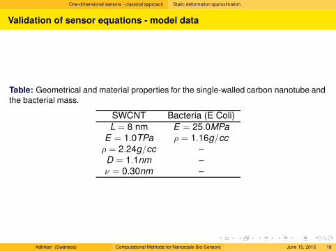
Validation of sensor equations - model data
Table: Geometrical and material properties for the single-walled carbon nanotube andthe bacterial mass.
SWCNT Bacteria (E Coli)
L = 8 nm E = 25.0MPa
E = 1.0TPa ρ = 1.16g/cc
ρ = 2.24g/cc –D = 1.1nm –ν = 0.30nm –
Adhikari (Swansea) Computational Methods for Nanoscale Bio-Sensors June 15, 2015 18
One-dimensional sensors - classical approach Static deformation approximation
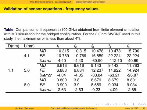
Validation of sensor equations - frequency values
Table: Comparison of frequencies (100 GHz) obtained from finite element simulationwith MD simulation for the bridged configuration. For the 8.0 nm SWCNT used in thisstudy, the maximum error is less than about 4%.
D(nm) L(nm) f1 f2 f3 f4 f5MD 10.315 10.315 10.478 10.478 15.796
4.1 FE 10.769 10.769 16.859 22.224 22.224%error -4.40 -4.40 -60.90 -112.10 -40.69MD 6.616 6.616 9.143 9.143 11.763
1.1 5.6 FE 6.883 6.884 12.237 14.922 14.924%error -4.04 -4.05 -33.84 -63.21 -26.87MD 3.800 3.8 8.679 8.679 8.801
8.0 FE 3.900 3.9 8.659 9.034 9.034%error -2.63 -2.63 -0.23 -4.09 -2.65
Adhikari (Swansea) Computational Methods for Nanoscale Bio-Sensors June 15, 2015 19
One-dimensional sensors - classical approach Static deformation approximation
Validation of sensor equations
10−2
10−1
100
10−2
10−1
100
101
102
Cha
nge
in m
ass:
M µ/ρ
A L
Frequency shift: ∆f 2π/α2β
exact analyticallinear approximationcubic approximationFE: bridgedFE: cantilevered
The general relationship between the normalized frequency-shift and normalized
added mass of the bio-particles in a SWCNT with effective density ρ, cross-section
area A and length L. Relationship between the frequency-shift and added mass of
bio-particles obtained from finite element simulation are also presented here to
visualize the effectiveness of analytical formulas.
Adhikari (Swansea) Computational Methods for Nanoscale Bio-Sensors June 15, 2015 20
One-dimensional sensors - classical approach Dynamic mode approximation
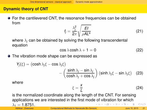
Dynamic theory of CNT
For the cantilevered CNT, the resonance frequencies can be obtainedfrom
fj =λ2
j
2π
√
EI
ρAL4(21)
where λj can be obtained by solving the following transcendentalequation
cosλ coshλ+ 1 = 0 (22)
The vibration mode shape can be expressed as
Yj (ξ) =(coshλjξ − cosλjξ
)
−(
sinhλj − sinλj
coshλj + cosλj
)(sinhλjξ − sinλjξ
)(23)
where
ξ =x
L(24)
is the normalized coordinate along the length of the CNT. For sensingapplications we are interested in the first mode of vibration for whichλ1 = 1.8751.
Adhikari (Swansea) Computational Methods for Nanoscale Bio-Sensors June 15, 2015 21
One-dimensional sensors - classical approach Dynamic mode approximation
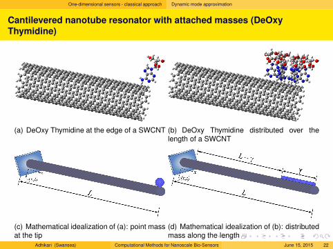
Cantilevered nanotube resonator with attached masses (DeOxy
Thymidine)
(a) DeOxy Thymidine at the edge of a SWCNT (b) DeOxy Thymidine distributed over thelength of a SWCNT
(c) Mathematical idealization of (a): point massat the tip
(d) Mathematical idealization of (b): distributedmass along the length
Adhikari (Swansea) Computational Methods for Nanoscale Bio-Sensors June 15, 2015 22
One-dimensional sensors - classical approach Dynamic mode approximation
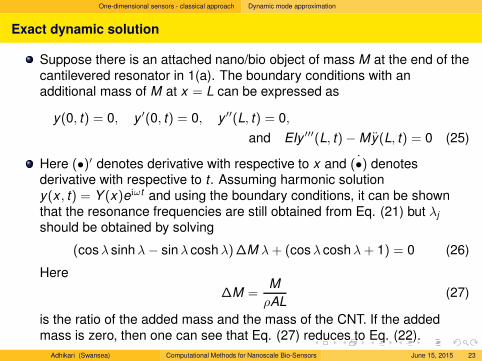
Exact dynamic solution
Suppose there is an attached nano/bio object of mass M at the end of thecantilevered resonator in 1(a). The boundary conditions with anadditional mass of M at x = L can be expressed as
y(0, t) = 0, y ′(0, t) = 0, y ′′(L, t) = 0,
and EIy ′′′(L, t)− My(L, t) = 0 (25)
Here (•)′ denotes derivative with respective to x and ˙(•) denotesderivative with respective to t. Assuming harmonic solutiony(x , t) = Y (x)eiωt and using the boundary conditions, it can be shownthat the resonance frequencies are still obtained from Eq. (21) but λj
should be obtained by solving
(cosλ sinhλ− sinλ coshλ)∆M λ+ (cosλ coshλ+ 1) = 0 (26)
Here
∆M =M
ρAL(27)
is the ratio of the added mass and the mass of the CNT. If the addedmass is zero, then one can see that Eq. (27) reduces to Eq. (22).
Adhikari (Swansea) Computational Methods for Nanoscale Bio-Sensors June 15, 2015 23
One-dimensional sensors - classical approach Dynamic mode approximation
Calibration Constants - energy approach
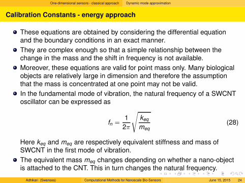
These equations are obtained by considering the differential equationand the boundary conditions in an exact manner.
They are complex enough so that a simple relationship between thechange in the mass and the shift in frequency is not available.
Moreover, these equations are valid for point mass only. Many biologicalobjects are relatively large in dimension and therefore the assumptionthat the mass is concentrated at one point may not be valid.
In the fundamental mode of vibration, the natural frequency of a SWCNToscillator can be expressed as
fn =1
2π
√
keq
meq(28)
Here keq and meq are respectively equivalent stiffness and mass ofSWCNT in the first mode of vibration.
The equivalent mass meq changes depending on whether a nano-objectis attached to the CNT. This in turn changes the natural frequency.
Adhikari (Swansea) Computational Methods for Nanoscale Bio-Sensors June 15, 2015 24
One-dimensional sensors - classical approach Dynamic mode approximation
Calibration Constants - energy approach
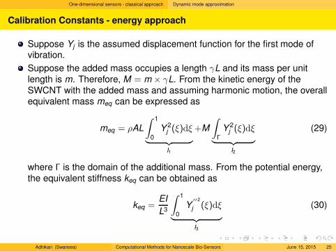
Suppose Yj is the assumed displacement function for the first mode ofvibration.
Suppose the added mass occupies a length γL and its mass per unitlength is m. Therefore, M = m × γL. From the kinetic energy of theSWCNT with the added mass and assuming harmonic motion, the overallequivalent mass meq can be expressed as
meq = ρAL
∫ 1
0
Y 2j (ξ)dξ
︸ ︷︷ ︸
I1
+M
∫
Γ
Y 2j (ξ)dξ
︸ ︷︷ ︸
I2
(29)
where Γ is the domain of the additional mass. From the potential energy,the equivalent stiffness keq can be obtained as
keq =EI
L3
∫ 1
0
Y′′2
j (ξ)dξ
︸ ︷︷ ︸
I3
(30)
Adhikari (Swansea) Computational Methods for Nanoscale Bio-Sensors June 15, 2015 25
One-dimensional sensors - classical approach Dynamic mode approximation
Calibration Constants - energy approach
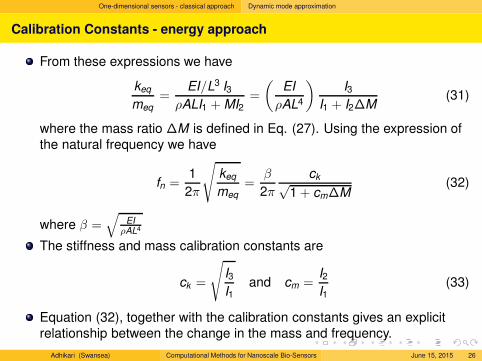
From these expressions we have
keq
meq=
EI/L3 I3
ρALI1 + MI2=
(EI
ρAL4
)I3
I1 + I2∆M(31)
where the mass ratio ∆M is defined in Eq. (27). Using the expression ofthe natural frequency we have
fn =1
2π
√
keq
meq=
β
2π
ck√1 + cm∆M
(32)
where β =√
EIρAL4
The stiffness and mass calibration constants are
ck =
√
I3
I1and cm =
I2
I1(33)
Equation (32), together with the calibration constants gives an explicitrelationship between the change in the mass and frequency.
Adhikari (Swansea) Computational Methods for Nanoscale Bio-Sensors June 15, 2015 26
One-dimensional sensors - classical approach Dynamic mode approximation
Calibration Constants - point mass
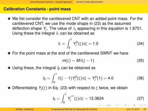
We fist consider the cantilevered CNT with an added point mass. For thecantilevered CNT, we use the mode shape in (23) as the assumeddeflection shape Yj . The value of λj appearing in this equation is 1.8751.Using these the integral I1 can be obtained as
I1 =
∫ 1
0
Y 2j (ξ)dξ = 1.0 (34)
For the point mass at the end of the cantilevered SWNT we have
m(ξ) = Mδ(ξ − 1) (35)
Using these, the integral I2 can be obtained as
I2 =
∫ 1
0
δ(ξ − 1)Y 2j (ξ)dξ = Y 2
j (1) = 4.0 (36)
Differentiating Yj(ξ) in Eq. (23) with respect to ξ twice, we obtain
I3 =
∫ 1
0
Y′′2
j (ξ)dξ = 12.3624 (37)
Adhikari (Swansea) Computational Methods for Nanoscale Bio-Sensors June 15, 2015 27
One-dimensional sensors - classical approach Dynamic mode approximation
Calibration Constants - distributed mass
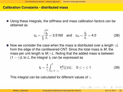
Using these integrals, the stiffness and mass calibration factors can beobtained as
ck =
√
I3
I1= 3.5160 and cm =
I2
I1= 4.0 (38)
Now we consider the case when the mass is distributed over a length γLfrom the edge of the cantilevered CNT. Since the total mass is M, themass per unit length is M/γL. Noting that the added mass is between(1 − γ)L to L, the integral I2 can be expressed as
I2 =1
γ
∫ 1
ξ=1−γ
Y 2j (ξ)dξ; 0 ≤ γ ≤ 1 (39)
This integral can be calculated for different values of γ.
Adhikari (Swansea) Computational Methods for Nanoscale Bio-Sensors June 15, 2015 28
One-dimensional sensors - classical approach Dynamic mode approximation
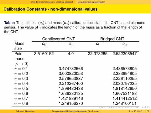
Calibration Constants - non-dimensional values
Table: The stiffness (ck ) and mass (cm) calibration constants for CNT based bio-nanosensor. The value of γ indicates the length of the mass as a fraction of the length ofthe CNT.
Cantilevered CNT Bridged CNTMasssize
ck cm ck cm
Pointmass(γ → 0)
3.5160152 4.0 22.373285 2.522208547
γ = 0.1 3.474732666 2.486573805γ = 0.2 3.000820053 2.383894805γ = 0.3 2.579653837 2.226110255γ = 0.4 2.212267400 2.030797235γ = 0.5 1.898480438 1.818142650γ = 0.6 1.636330135 1.607531183γ = 0.7 1.421839146 1.414412512γ = 0.8 1.249156270 1.248100151
Adhikari (Swansea) Computational Methods for Nanoscale Bio-Sensors June 15, 2015 29
One-dimensional sensors - classical approach Dynamic mode approximation
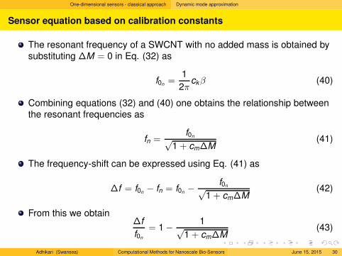
Sensor equation based on calibration constants
The resonant frequency of a SWCNT with no added mass is obtained bysubstituting ∆M = 0 in Eq. (32) as
f0n=
1
2πckβ (40)
Combining equations (32) and (40) one obtains the relationship betweenthe resonant frequencies as
fn =f0n√
1 + cm∆M(41)
The frequency-shift can be expressed using Eq. (41) as
∆f = f0n− fn = f0n
− f0n√1 + cm∆M
(42)
From this we obtain∆f
f0n
= 1 − 1√1 + cm∆M
(43)
Adhikari (Swansea) Computational Methods for Nanoscale Bio-Sensors June 15, 2015 30
One-dimensional sensors - classical approach Dynamic mode approximation
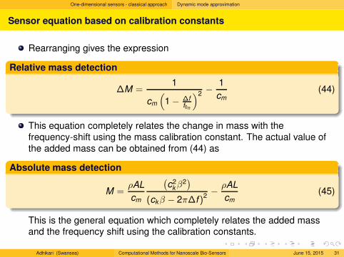
Sensor equation based on calibration constants
Rearranging gives the expression
Relative mass detection
∆M =1
cm
(
1 − ∆ff0n
)2− 1
cm(44)
This equation completely relates the change in mass with thefrequency-shift using the mass calibration constant. The actual value ofthe added mass can be obtained from (44) as
Absolute mass detection
M =ρAL
cm
(c2
kβ2)
(ckβ − 2π∆f )2− ρAL
cm(45)
This is the general equation which completely relates the added massand the frequency shift using the calibration constants.
Adhikari (Swansea) Computational Methods for Nanoscale Bio-Sensors June 15, 2015 31
One-dimensional sensors - classical approach Dynamic mode approximation
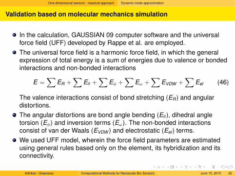
Validation based on molecular mechanics simulation
In the calculation, GAUSSIAN 09 computer software and the universalforce field (UFF) developed by Rappe et al. are employed.
The universal force field is a harmonic force field, in which the generalexpression of total energy is a sum of energies due to valence or bondedinteractions and non-bonded interactions
E =∑
ER +∑
Eθ +∑
Eφ +∑
Eω +∑
EVDW +∑
Eel (46)
The valence interactions consist of bond stretching (ER) and angulardistortions.
The angular distortions are bond angle bending (Eθ), dihedral angletorsion (Eφ) and inversion terms (Eω). The non-bonded interactionsconsist of van der Waals (EVDW ) and electrostatic (Eel ) terms.
We used UFF model, wherein the force field parameters are estimatedusing general rules based only on the element, its hybridization and itsconnectivity.
Adhikari (Swansea) Computational Methods for Nanoscale Bio-Sensors June 15, 2015 32
One-dimensional sensors - classical approach Dynamic mode approximation
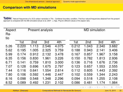
Comparison with MD simulations
Table: Natural frequencies of a (5,5) carbon nanotube in THz - Cantilever boundary condition. First four natural frequencies obtained from the presentapproach is compared with the MD simulation [Duan et al, 2007 - J. App. Phy] for different values of the aspect ratio.
AspectRa-tio
Present analysis MD simulation
1st 2nd 3rd 4th 1st 2nd 3rd 4th5.26 0.220 1.113 2.546 4.075 0.212 1.043 2.340 3.6825.62 0.195 1.005 2.325 3.759 0.188 0.943 2.141 3.4065.99 0.174 0.912 2.132 3.478 0.167 0.857 1.967 3.1586.35 0.156 0.830 1.961 3.226 0.150 0.782 1.813 2.9366.71 0.141 0.759 1.810 3.000 0.136 0.716 1.676 2.7367.07 0.128 0.696 1.675 2.797 0.123 0.657 1.553 2.5557.44 0.116 0.641 1.554 2.614 0.112 0.605 1.443 2.3927.80 0.106 0.592 1.446 2.447 0.102 0.559 1.344 2.2438.16 0.098 0.548 1.348 2.296 0.094 0.518 1.255 2.1088.52 0.089 0.492 1.231 2.102 0.086 0.481 1.174 1.984
Adhikari (Swansea) Computational Methods for Nanoscale Bio-Sensors June 15, 2015 33
One-dimensional sensors - classical approach Dynamic mode approximation
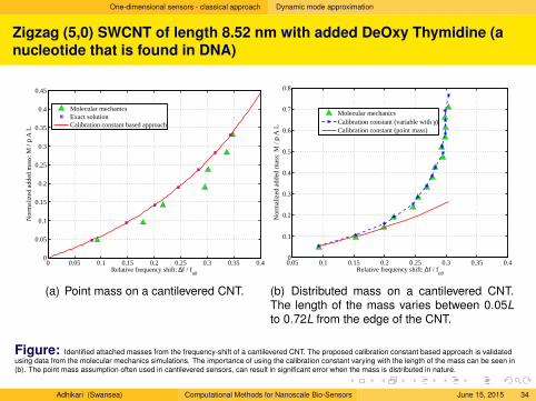
Zigzag (5,0) SWCNT of length 8.52 nm with added DeOxy Thymidine (a
nucleotide that is found in DNA)
0 0.05 0.1 0.15 0.2 0.25 0.3 0.35 0.40
0.05
0.1
0.15
0.2
0.25
0.3
0.35
0.4
0.45
Nor
mal
ized
add
ed m
ass:
M / ρ A
L
Relative frequency shift: ∆f / fn0
Molecular mechanicsExact solutionCalibration constant based approach
(a) Point mass on a cantilevered CNT.
0.05 0.1 0.15 0.2 0.25 0.3 0.35 0.40
0.1
0.2
0.3
0.4
0.5
0.6
0.7
0.8
Nor
mal
ized
add
ed m
ass:
M / ρ A
LRelative frequency shift: ∆f / f
n0
Molecular mechanicsCalibration constant (variable with γ)Calibration constant (point mass)
(b) Distributed mass on a cantilevered CNT.The length of the mass varies between 0.05Lto 0.72L from the edge of the CNT.
Figure: Identified attached masses from the frequency-shift of a cantilevered CNT. The proposed calibration constant based approach is validatedusing data from the molecular mechanics simulations. The importance of using the calibration constant varying with the length of the mass can be seen in(b). The point mass assumption often used in cantilevered sensors, can result in significant error when the mass is distributed in nature.
Adhikari (Swansea) Computational Methods for Nanoscale Bio-Sensors June 15, 2015 34
One-dimensional sensors - classical approach Dynamic mode approximation
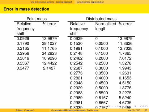
Error in mass detection
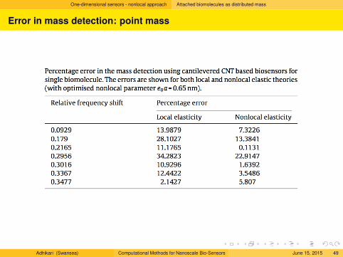
Point mass Distributed massRelativefrequencyshift
% error Relativefrequencyshift
Normalizedlength
% error
0.0929 13.9879 0.0929 0 13.98790.1790 28.1027 0.1530 0.0500 11.86260.2165 11.1765 0.1991 0.1000 13.70380.2956 34.2823 0.2148 0.1500 1.78650.3016 10.9296 0.2462 0.2000 7.01720.3367 12.4422 0.2542 0.2500 1.32780.3477 2.1427 0.2687 0.3000 1.9943
0.2773 0.3500 1.26310.2821 0.4000 0.16530.2948 0.4500 4.51500.2929 0.5000 1.37760.2983 0.5500 3.22750.2989 0.6167 5.52400.2981 0.6667 4.67350.3039 0.7167 7.9455
Adhikari (Swansea) Computational Methods for Nanoscale Bio-Sensors June 15, 2015 35
One-dimensional sensors - classical approach Dynamic mode approximation
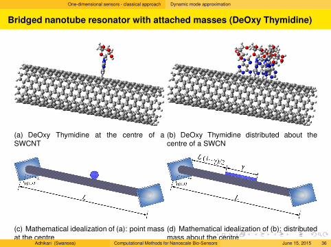
Bridged nanotube resonator with attached masses (DeOxy Thymidine)
(a) DeOxy Thymidine at the centre of aSWCNT
(b) DeOxy Thymidine distributed about thecentre of a SWCN
(c) Mathematical idealization of (a): point massat the centre
(d) Mathematical idealization of (b): distributedmass about the centre
Adhikari (Swansea) Computational Methods for Nanoscale Bio-Sensors June 15, 2015 36
One-dimensional sensors - classical approach Dynamic mode approximation
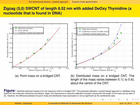
Zigzag (5,0) SWCNT of length 8.52 nm with added DeOxy Thymidine (a
nucleotide that is found in DNA)
0 0.05 0.1 0.15 0.2 0.25 0.3 0.350
0.05
0.1
0.15
0.2
0.25
0.3
0.35
0.4
0.45
Nor
mal
ized
add
ed m
ass:
M / ρ A
L
Relative frequency shift: ∆f / fn0
Molecular mechanicsExact solutionCalibration constant based approach
(a) Point mass on a bridged CNT.
0.05 0.1 0.15 0.2 0.25 0.3 0.35 0.40
0.1
0.2
0.3
0.4
0.5
0.6
0.7
0.8
Nor
mal
ized
add
ed m
ass:
M / ρ A
LRelative frequency shift: ∆f / f
n0
Molecular mechanicsCalibration constant (variable with γ)Calibration constant (point mass)
(b) Distributed mass on a bridged CNT. Thelength of the mass varies between 0.1L to 0.6Labout the centre of the CNT.
Figure: Identified attached masses from the frequency-shift of a bridged CNT. The proposed calibration constant based approach is validated usingdata from the molecular mechanics simulations. Again, the importance of using the calibration constant varying with the length of the mass can be seen in(b). However, the difference between the point mass and distributed mass assumption is not as significant as the cantilevered case.
Adhikari (Swansea) Computational Methods for Nanoscale Bio-Sensors June 15, 2015 37
One-dimensional sensors - classical approach Dynamic mode approximation
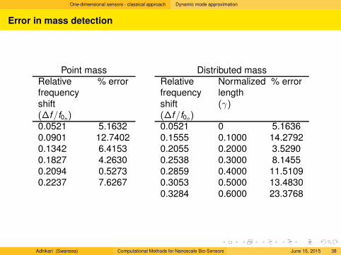
Error in mass detection
Point mass Distributed massRelativefrequencyshift(∆f/f0n
)
% error Relativefrequencyshift(∆f/f0n
)
Normalizedlength(γ)
% error
0.0521 5.1632 0.0521 0 5.16360.0901 12.7402 0.1555 0.1000 14.27920.1342 6.4153 0.2055 0.2000 3.52900.1827 4.2630 0.2538 0.3000 8.14550.2094 0.5273 0.2859 0.4000 11.51090.2237 7.6267 0.3053 0.5000 13.4830
0.3284 0.6000 23.3768
Adhikari (Swansea) Computational Methods for Nanoscale Bio-Sensors June 15, 2015 38
One-dimensional sensors - nonlocal approach
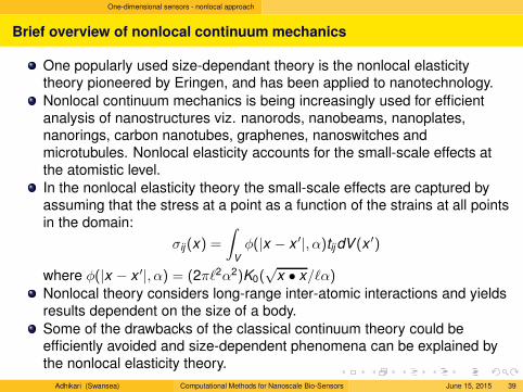
Brief overview of nonlocal continuum mechanics
One popularly used size-dependant theory is the nonlocal elasticitytheory pioneered by Eringen, and has been applied to nanotechnology.
Nonlocal continuum mechanics is being increasingly used for efficientanalysis of nanostructures viz. nanorods, nanobeams, nanoplates,nanorings, carbon nanotubes, graphenes, nanoswitches andmicrotubules. Nonlocal elasticity accounts for the small-scale effects atthe atomistic level.
In the nonlocal elasticity theory the small-scale effects are captured byassuming that the stress at a point as a function of the strains at all pointsin the domain:
σij (x) =
∫
V
φ(|x − x ′|, α)tij dV (x ′)
where φ(|x − x ′|, α) = (2πℓ2α2)K0(√
x • x/ℓα)
Nonlocal theory considers long-range inter-atomic interactions and yieldsresults dependent on the size of a body.
Some of the drawbacks of the classical continuum theory could beefficiently avoided and size-dependent phenomena can be explained bythe nonlocal elasticity theory.
Adhikari (Swansea) Computational Methods for Nanoscale Bio-Sensors June 15, 2015 39
One-dimensional sensors - nonlocal approach
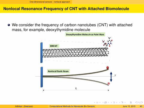
Nonlocal Resonance Frequency of CNT with Attached Biomolecule
We consider the frequency of carbon nanotubes (CNT) with attachedmass, for example, deoxythymidine molecule
Adhikari (Swansea) Computational Methods for Nanoscale Bio-Sensors June 15, 2015 40
One-dimensional sensors - nonlocal approach Attached biomolecules as point mass
Nonlocal Resonance Frequency of CNT with Attached biomolecule
For the bending vibration of a nonlocal damped beam, the equation ofmotion of free vibration can be expressed by
EI∂4V (x , t)
∂x4+ m
(
1 − (e0a)2 ∂2
∂x2
){∂2V (x , t)
∂t2
}
= 0 (47)
In the fundamental mode of vibration, the natural frequency of a nonlocalSWCNT oscillator can be expressed as
fn =1
2π
√
keq
meq(48)
Here keq and meq are respectively equivalent stiffness and mass ofSWCNT in the first mode of vibration.
Adhikari (Swansea) Computational Methods for Nanoscale Bio-Sensors June 15, 2015 41
One-dimensional sensors - nonlocal approach Attached biomolecules as point mass
Nonlocal resonance frequency with attached point biomolecule
Following the energy approach, the natural frequency can be expressedas
fn =1
2π
√
keq
meq=
β
2π
ck√
1 + cnlθ2 + cm∆M(49)
where
β =
√
EI
ρAL4, θ =
e0a
Land ∆M =
M
ρAL(50)
The stiffness, mass and nonlocal calibration constants are
ck =
√
140
11, cm =
140
33and cnl =
56
11(51)
Equation (49), together with the calibration constants gives an explicitrelationship between the change in the mass and frequency.
Adhikari (Swansea) Computational Methods for Nanoscale Bio-Sensors June 15, 2015 42
One-dimensional sensors - nonlocal approach Attached biomolecules as point mass
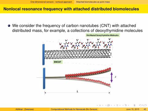
Nonlocal resonance frequency with attached distributed biomolecules
We consider the frequency of carbon nanotubes (CNT) with attacheddistributed mass, for example, a collections of deoxythymidine molecules
Adhikari (Swansea) Computational Methods for Nanoscale Bio-Sensors June 15, 2015 43
One-dimensional sensors - nonlocal approach Attached biomolecules as distributed mass
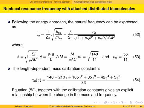
Nonlocal resonance frequency with attached distributed biomolecules
Following the energy approach, the natural frequency can be expressedas
fn =1
2π
√
keq
meq=
β
2π
ck√
1 + cnlθ2 + cm(γ)∆M(52)
where
β =
√
EI
ρAL4, θ =
e0a
L,∆M =
M
ρAL, ck =
√
140
11and cnl =
56
11(53)
The length-dependent mass calibration constant is
cm(γ) =140 − 210γ + 105γ2 + 35γ3 − 42γ4 + 5γ6
33(54)
Equation (52), together with the calibration constants gives an explicitrelationship between the change in the mass and frequency.
Adhikari (Swansea) Computational Methods for Nanoscale Bio-Sensors June 15, 2015 44
One-dimensional sensors - nonlocal approach Attached biomolecules as distributed mass
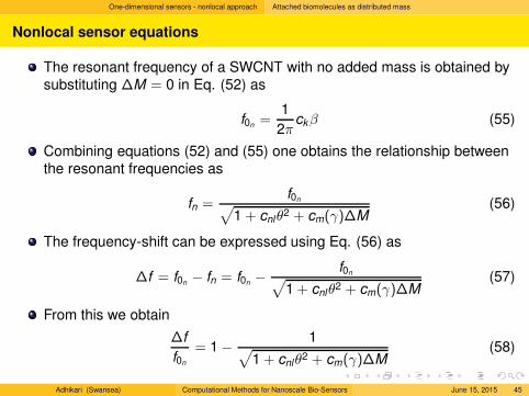
Nonlocal sensor equations
The resonant frequency of a SWCNT with no added mass is obtained bysubstituting ∆M = 0 in Eq. (52) as
f0n=
1
2πckβ (55)
Combining equations (52) and (55) one obtains the relationship betweenthe resonant frequencies as
fn =f0n
√
1 + cnlθ2 + cm(γ)∆M(56)
The frequency-shift can be expressed using Eq. (56) as
∆f = f0n− fn = f0n
− f0n√
1 + cnlθ2 + cm(γ)∆M(57)
From this we obtain
∆f
f0n
= 1 − 1√
1 + cnlθ2 + cm(γ)∆M(58)
Adhikari (Swansea) Computational Methods for Nanoscale Bio-Sensors June 15, 2015 45
One-dimensional sensors - nonlocal approach Attached biomolecules as distributed mass
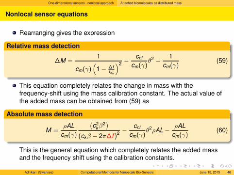
Nonlocal sensor equations
Rearranging gives the expression
Relative mass detection
∆M =1
cm(γ)(
1 − ∆ff0n
)2− cnl
cm(γ)θ2 − 1
cm(γ)(59)
This equation completely relates the change in mass with thefrequency-shift using the mass calibration constant. The actual value ofthe added mass can be obtained from (59) as
Absolute mass detection
M =ρAL
cm(γ)
(c2
kβ2)
(ckβ − 2π∆f )2− cnl
cm(γ)θ2ρAL − ρAL
cm(γ)(60)
This is the general equation which completely relates the added massand the frequency shift using the calibration constants.
Adhikari (Swansea) Computational Methods for Nanoscale Bio-Sensors June 15, 2015 46
One-dimensional sensors - nonlocal approach Attached biomolecules as distributed mass
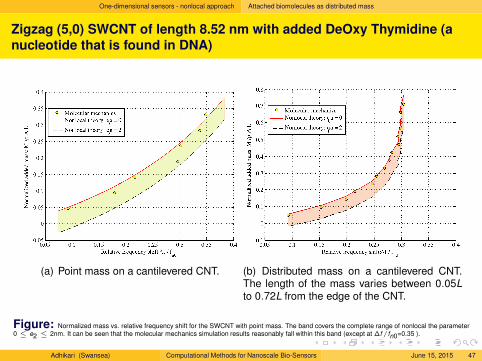
Zigzag (5,0) SWCNT of length 8.52 nm with added DeOxy Thymidine (a
nucleotide that is found in DNA)
(a) Point mass on a cantilevered CNT. (b) Distributed mass on a cantilevered CNT.The length of the mass varies between 0.05Lto 0.72L from the edge of the CNT.
Figure: Normalized mass vs. relative frequency shift for the SWCNT with point mass. The band covers the complete range of nonlocal the parameter0 ≤ e2 ≤ 2nm. It can be seen that the molecular mechanics simulation results reasonably fall within this band (except at ∆f/fn0=0.35 ).
Adhikari (Swansea) Computational Methods for Nanoscale Bio-Sensors June 15, 2015 47
One-dimensional sensors - nonlocal approach Attached biomolecules as distributed mass
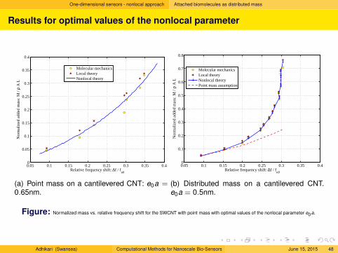
Results for optimal values of the nonlocal parameter
0.05 0.1 0.15 0.2 0.25 0.3 0.35 0.40
0.05
0.1
0.15
0.2
0.25
0.3
0.35
0.4
Nor
mal
ized
add
ed m
ass:
M / ρ A
L
Relative frequency shift: ∆f / fn0
Molecular mechanicsLocal theoryNonlocal theory
(a) Point mass on a cantilevered CNT: e0a =0.65nm.
0.05 0.1 0.15 0.2 0.25 0.3 0.35 0.40
0.1
0.2
0.3
0.4
0.5
0.6
0.7
0.8
Nor
mal
ized
add
ed m
ass:
M / ρ A
LRelative frequency shift: ∆f / f
n0
Molecular mechanicsLocal theoryNonlocal theoryPoint mass assumption
(b) Distributed mass on a cantilevered CNT.e0a = 0.5nm.
Figure: Normalized mass vs. relative frequency shift for the SWCNT with point mass with optimal values of the nonlocal parameter e0a.
Adhikari (Swansea) Computational Methods for Nanoscale Bio-Sensors June 15, 2015 48
One-dimensional sensors - nonlocal approach Attached biomolecules as distributed mass
Error in mass detection: point mass
Adhikari (Swansea) Computational Methods for Nanoscale Bio-Sensors June 15, 2015 49
One-dimensional sensors - nonlocal approach Attached biomolecules as distributed mass
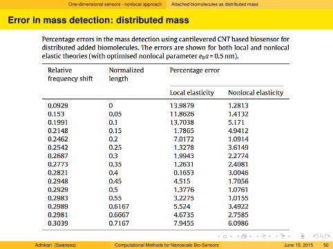
Error in mass detection: distributed mass
Adhikari (Swansea) Computational Methods for Nanoscale Bio-Sensors June 15, 2015 50
Two-dimensional sensors - classical approach
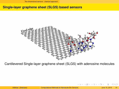
Single-layer graphene sheet (SLGS) based sensors
Fixed edge
Cantilevered Single-layer graphene sheet (SLGS) with adenosine molecules
Adhikari (Swansea) Computational Methods for Nanoscale Bio-Sensors June 15, 2015 51
Two-dimensional sensors - classical approach
Resonant frequencies of SLGS with attached mass
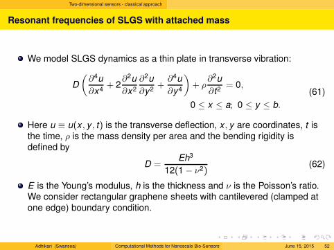
We model SLGS dynamics as a thin plate in transverse vibration:
D
(∂4u
∂x4+ 2
∂2u
∂x2
∂2u
∂y2+
∂4u
∂y4
)
+ ρ∂2u
∂t2= 0,
0 ≤ x ≤ a; 0 ≤ y ≤ b.
(61)
Here u ≡ u(x , y , t) is the transverse deflection, x , y are coordinates, t isthe time, ρ is the mass density per area and the bending rigidity isdefined by
D =Eh3
12(1 − ν2)(62)
E is the Young’s modulus, h is the thickness and ν is the Poisson’s ratio.We consider rectangular graphene sheets with cantilevered (clamped atone edge) boundary condition.
Adhikari (Swansea) Computational Methods for Nanoscale Bio-Sensors June 15, 2015 52
Two-dimensional sensors - classical approach
Resonant frequencies of SLGS
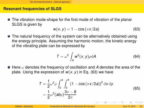
The vibration mode-shape for the first mode of vibration of the planarSLGS is given by
w(x , y) = 1 − cos (πx/2a) (63)
The natural frequency of the system can be alternatively obtained usingthe energy principle. Assuming the harmonic motion, the kinetic energyof the vibrating plate can be expressed by
T = ω2
∫
A
w2(x , y)ρdA (64)
Here ω denotes the frequency of oscillation and A denotes the area of theplate. Using the expression of w(x , y) in Eq. (63) we have
T =1
2ω2ρ
∫ a
0
∫ b
0
(1 − cos (πx/2a))2dx dy
=1
2ω2(abρ)
3π − 8
2π
(65)
Adhikari (Swansea) Computational Methods for Nanoscale Bio-Sensors June 15, 2015 53
Two-dimensional sensors - classical approach
Resonant frequencies of SLGS
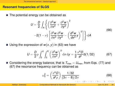
The potential energy can be obtained as
U =D
2
∫
A
{(∂2w
∂x2+
∂2w
∂y2
)2
−2(1 − ν)
[
∂2w
∂x2
∂2w
∂y2−(
d2w
dx2y
)2]}
dA
(66)
Using the expression of w(x , y) in (63) we have
U =D
2ρ
∫ a
0
∫ b
0
(∂2w
∂x2
)2
dx dy =1
2
π4D
a3b(1/32) (67)
Considering the energy balance, that is Tmax = Umax, from Eqs. (77) and(67) the resonance frequency can be obtained as
ω20 =
(π4D
a4ρ
)1/32
(3π − 8)/2π(68)
Adhikari (Swansea) Computational Methods for Nanoscale Bio-Sensors June 15, 2015 54
Two-dimensional sensors - classical approach
Resonant frequencies of SLGS with attached mass
��
��
a
b
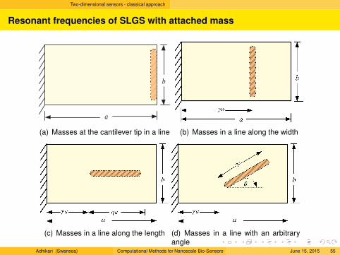
(a) Masses at the cantilever tip in a line (b) Masses in a line along the width
(c) Masses in a line along the length (d) Masses in a line with an arbitraryangle
Adhikari (Swansea) Computational Methods for Nanoscale Bio-Sensors June 15, 2015 55
Two-dimensional sensors - classical approach
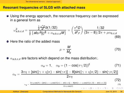
Resonant frequencies of SLGS with attached mass
Using the energy approach, the resonance frequency can be expressedin a general form as
ω2a,b,c,d =
12π4Da3 b(1/32)
12
{abρ 3π−8
2π+ αa,b,c,dM
} =
(π4D
a4ρ
)1/32
(3π − 8)/2π + µαb,c,d
(69)
Here the ratio of the added mass
µ =M
Mg(70)
αa,b,c,d are factors which depend on the mass distribution:.
αa = 1, αb = (1 − cos(πγ/2))2 (71)
αc =3πη + [sin((γ + η)π) − sin(γπ)]− 8[sin((γ + η)π/2)− sin(γπ/2)]
2πη(72)
αd =3πη cos(θ) + [sin((γ + η cos(θ))π) − sin(γπ)] − 8[sin((γ + η cos(θ))π/2) − sin(γπ/2)]
2πη cos(θ)(73)
Adhikari (Swansea) Computational Methods for Nanoscale Bio-Sensors June 15, 2015 56
Two-dimensional sensors - classical approach
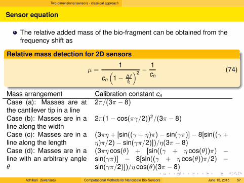
Sensor equation
The relative added mass of the bio-fragment can be obtained from thefrequency shift as
Relative mass detection for 2D sensors
µ =1
cn
(
1 − ∆ff0
)2− 1
cn(74)
Mass arrangement Calibration constant cn
Case (a): Masses are atthe cantilever tip in a line
2π/(3π − 8)
Case (b): Masses are in aline along the width
2π(1 − cos(πγ/2))2/(3π − 8)
Case (c): Masses are in aline along the length
(3πη + [sin((γ + η)π) − sin(γπ)] − 8[sin((γ +η)π/2)− sin(γπ/2)])/η(3π − 8)
Case (d): Masses are in aline with an arbitrary angleθ
(3πη cos(θ) + [sin((γ + η cos(θ))π) −sin(γπ)] − 8[sin((γ + η cos(θ))π/2) −sin(γπ/2)])/η cos(θ)(3π − 8)
Adhikari (Swansea) Computational Methods for Nanoscale Bio-Sensors June 15, 2015 57
Two-dimensional sensors - classical approach
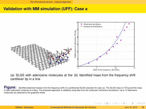
Validation with MM simulation (UFF): Case a
Fixed edge
(a) SLGS with adenosine molecules at thecantilever tip in a line
0 5 10 150
1
2
3
4
5
6
Add
ed m
ass
of A
deno
sine
: M (
zg)
Shift in the frequency: ∆f (GHz)
Molecular mechanicsAnalytical formulation
(b) Identified mass from the frequency shift
Figure: Identified attached masses from the frequency-shift of a cantilevered SLGS resonator for case (a). The SLGS mass is 7.57zg and the massof each adenosine molecule is 0.44zg. The proposed approach is validated using data from the molecular mechanics simulations. Up to 12 adenosinemolecules are attached to the graphene sheet.
Adhikari (Swansea) Computational Methods for Nanoscale Bio-Sensors June 15, 2015 58
Two-dimensional sensors - classical approach
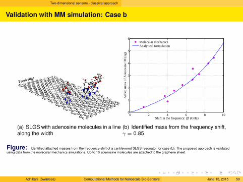
Validation with MM simulation: Case b
Fixed edge
(a) SLGS with adenosine molecules in a linealong the width
0 2 4 6 8 100
1
2
3
4
5
6
Add
ed m
ass
of A
deno
sine
: M (
zg)
Shift in the frequency: ∆f (GHz)
Molecular mechanicsAnalytical formulation
(b) Identified mass from the frequency shift,γ = 0.85
Figure: Identified attached masses from the frequency-shift of a cantilevered SLGS resonator for case (b). The proposed approach is validatedusing data from the molecular mechanics simulations. Up to 10 adenosine molecules are attached to the graphene sheet.
Adhikari (Swansea) Computational Methods for Nanoscale Bio-Sensors June 15, 2015 59
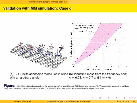
Two-dimensional sensors - classical approach
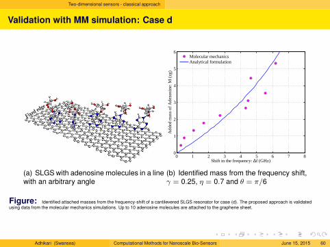
Validation with MM simulation: Case d
Fixed edge
(a) SLGS with adenosine molecules in a linewith an arbitrary angle
0 1 2 3 4 5 6 7 80
1
2
3
4
5
6
Add
ed m
ass
of A
deno
sine
: M (
zg)
Shift in the frequency: ∆f (GHz)
Molecular mechanicsAnalytical formulation
(b) Identified mass from the frequency shift,γ = 0.25, η = 0.7 and θ = π/6
Figure: Identified attached masses from the frequency-shift of a cantilevered SLGS resonator for case (d). The proposed approach is validatedusing data from the molecular mechanics simulations. Up to 10 adenosine molecules are attached to the graphene sheet.
Adhikari (Swansea) Computational Methods for Nanoscale Bio-Sensors June 15, 2015 60
Two-dimensional sensors - nonlocal approach
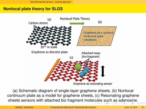
Nonlocal plate theory for SLGS
(a) Schematic diagram of single-layer graphene sheets, (b) Nonlocalcontinuum plate as a model for graphene sheets, (c) Resonating graphenesheets sensors with attached bio fragment molecules such as adenosine.
Adhikari (Swansea) Computational Methods for Nanoscale Bio-Sensors June 15, 2015 61
Two-dimensional sensors - nonlocal approach
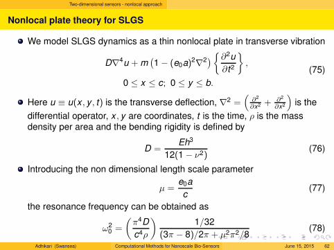
Nonlocal plate theory for SLGS
We model SLGS dynamics as a thin nonlocal plate in transverse vibration
D∇4u + m(1 − (e0a)2∇2
){∂2u
∂t2
}
,
0 ≤ x ≤ c; 0 ≤ y ≤ b.
(75)
Here u ≡ u(x , y , t) is the transverse deflection, ∇2 =(
∂2
∂x2 + ∂2
∂x2
)
is the
differential operator, x , y are coordinates, t is the time, ρ is the massdensity per area and the bending rigidity is defined by
D =Eh3
12(1 − ν2)(76)
Introducing the non dimensional length scale parameter
µ =e0a
c(77)
the resonance frequency can be obtained as
ω20 =
(π4D
c4ρ
)1/32
(3π − 8)/2π + µ2π2/8(78)
Adhikari (Swansea) Computational Methods for Nanoscale Bio-Sensors June 15, 2015 62
Two-dimensional sensors - nonlocal approach
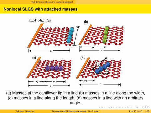
Nonlocal SLGS with attached masses
(a) Masses at the cantilever tip in a line (b) masses in a line along the width,(c) masses in a line along the length, (d) masses in a line with an arbitrary
angle.
Adhikari (Swansea) Computational Methods for Nanoscale Bio-Sensors June 15, 2015 63
Two-dimensional sensors - nonlocal approach
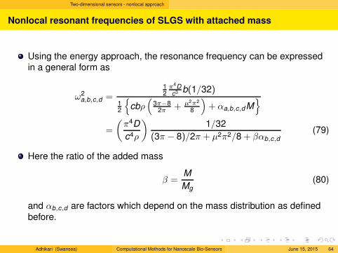
Nonlocal resonant frequencies of SLGS with attached mass
Using the energy approach, the resonance frequency can be expressedin a general form as
ω2a,b,c,d =
12π4Dc3 b(1/32)
12
{
cbρ(
3π−82π + µ2π2
8
)
+ αa,b,c,dM}
=
(π4D
c4ρ
)1/32
(3π − 8)/2π + µ2π2/8 + βαb,c,d
(79)
Here the ratio of the added mass
β =M
Mg(80)
and αb,c,d are factors which depend on the mass distribution as definedbefore.
Adhikari (Swansea) Computational Methods for Nanoscale Bio-Sensors June 15, 2015 64
Two-dimensional sensors - nonlocal approach
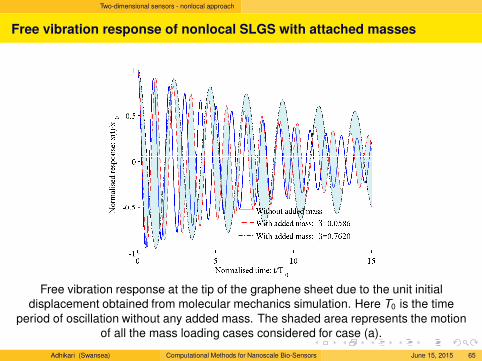
Free vibration response of nonlocal SLGS with attached masses
Free vibration response at the tip of the graphene sheet due to the unit initialdisplacement obtained from molecular mechanics simulation. Here T0 is the time
period of oscillation without any added mass. The shaded area represents the motionof all the mass loading cases considered for case (a).
Adhikari (Swansea) Computational Methods for Nanoscale Bio-Sensors June 15, 2015 65
Two-dimensional sensors - nonlocal approach
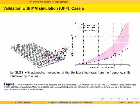
Validation with MM simulation (UFF): Case a
Fixed edge
(a) SLGS with adenosine molecules at thecantilever tip in a line
(b) Identified mass from the frequency shift
Figure: Identified attached masses from the frequency-shift of a cantilevered SLGS resonator for case (a). The SLGS mass is 7.57zg and the massof each adenosine molecule is 0.44zg. The proposed approach is validated using data from the molecular mechanics simulations. Up to 12 adenosinemolecules are attached to the graphene sheet.
Adhikari (Swansea) Computational Methods for Nanoscale Bio-Sensors June 15, 2015 66
Two-dimensional sensors - nonlocal approach
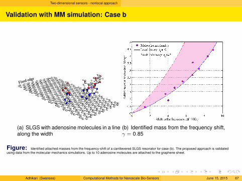
Validation with MM simulation: Case b
Fixed edge
(a) SLGS with adenosine molecules in a linealong the width
(b) Identified mass from the frequency shift,γ = 0.85
Figure: Identified attached masses from the frequency-shift of a cantilevered SLGS resonator for case (b). The proposed approach is validatedusing data from the molecular mechanics simulations. Up to 10 adenosine molecules are attached to the graphene sheet.
Adhikari (Swansea) Computational Methods for Nanoscale Bio-Sensors June 15, 2015 67
Two-dimensional sensors - nonlocal approach
Validation with MM simulation: Case d
Fixed edge
(a) SLGS with adenosine molecules in a linewith an arbitrary angle
(b) Identified mass from the frequency shift,γ = 0.25, η = 0.7 and θ = π/6
Figure: Identified attached masses from the frequency-shift of a cantilevered SLGS resonator for case (d). The proposed approach is validatedusing data from the molecular mechanics simulations. Up to 10 adenosine molecules are attached to the graphene sheet.
Adhikari (Swansea) Computational Methods for Nanoscale Bio-Sensors June 15, 2015 68
Conclusions
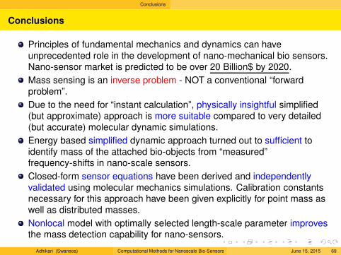
Conclusions
Principles of fundamental mechanics and dynamics can haveunprecedented role in the development of nano-mechanical bio sensors.Nano-sensor market is predicted to be over 20 Billion$ by 2020.
Mass sensing is an inverse problem - NOT a conventional “forwardproblem”.
Due to the need for “instant calculation”, physically insightful simplified(but approximate) approach is more suitable compared to very detailed(but accurate) molecular dynamic simulations.
Energy based simplified dynamic approach turned out to sufficient toidentify mass of the attached bio-objects from “measured”frequency-shifts in nano-scale sensors.
Closed-form sensor equations have been derived and independentlyvalidated using molecular mechanics simulations. Calibration constantsnecessary for this approach have been given explicitly for point mass aswell as distributed masses.
Nonlocal model with optimally selected length-scale parameter improvesthe mass detection capability for nano-sensors.
Adhikari (Swansea) Computational Methods for Nanoscale Bio-Sensors June 15, 2015 69
Our related publications
[1] Chowdhury, R., Adhikari, S., and Mitchell, J., “Vibrating carbon nanotube based bio-sensors,” Physica E: Low-Dimensional Systems and
Nanostructures, Vol. 42, No. 2, December 2009, pp. 104–109.[2] Adhikari, S. and Chowdhury, R., “The calibration of carbon nanotube based bio-nano sensors,” Journal of Applied Physics, Vol. 107, No. 12, 2010,
pp. 124322:1–8.[3] Chowdhury, R., Adhikari, S., Rees, P., Scarpa, F., and Wilks, S. P., “Graphene based bio-sensor using transport properties,” Physical Review B,
Vol. 83, No. 4, 2011, pp. 045401:1–8.[4] Chowdhury, R. and Adhikari, S., “Boron nitride nanotubes as zeptogram-scale bio-nano sensors: Theoretical investigations,” IEEE Transactions on
Nanotechnology , Vol. 10, No. 4, 2011, pp. 659–667.[5] Murmu, T. and Adhikari, S., “Nonlocal frequency analysis of nanoscale biosensors,” Sensors & Actuators: A. Physical , Vol. 173, No. 1, 2012,
pp. 41–48.[6] Adhikari, S. and Chowdhury, R., “Zeptogram sensing from gigahertz vibration: Graphene based nanosensor,” Physica E: Low-dimensional Systems
and Nanostructures, Vol. 44, No. 7-8, 2012, pp. 1528–1534.[7] Adhikari, S. and Murmu, T., “Nonlocal mass nanosensors based on vibrating monolayer graphene sheets,” Sensors & Actuators: B. Chemical ,
Vol. 188, No. 11, 2013, pp. 1319–1327.[8] Kam, K., Scarpa, F., Adhikari, S., and Chowdhury, R., “Graphene nanofilm as pressure and force sensor: a mechanical analysis,” Physica Status
Solidi B, Vol. 250, No. 10, 2013, pp. 2085–2089.[9] Sheady, Z. and Adhikari, S., “Cantilevered biosensors: Mass and rotary inertia identification,” Proceedings of the 11th Annual International Workshop
on Nanomechanical Sensing (NMC 2014), Madrid, Spain, May 2014.[10] Clarke, E. and Adhikari, S., “Two is better than one: Weakly coupled nano cantilevers show ultra-sensitivity of mass detection,” Proceedings of the
11th Annual International Workshop on Nanomechanical Sensing (NMC 2014), Madrid, Spain, May 2014.[11] Karlicic, D., Kozic, P., Adhikari, S., Cajic, M., Murmu, T., and Lazarevic, M., “Nonlocal biosensor based on the damped vibration of single-layer
graphene influenced by in-plane magnetic field,” International Journal of Mechanical Sciences, Vol. 96-97, No. 6, 2015, pp. 101–109.
Adhikari (Swansea) Computational Methods for Nanoscale Bio-Sensors June 15, 2015 69