computational methods for oil recovery - boston university · computational methods for oil...
TRANSCRIPT

Math, Num and Comp Models References
Computational Methods for Oil RecoveryPASI: Scientific Computing in the Americas
The Challenge of Massive Parallelism
Luis M. de la Cruz Salas
Instituto de Geofısica
Universidad Nacional Autonoma de Mexico
January 2011
Valparaıso, Chile
Comp EOR LMCS 1 / 76

Math, Num and Comp Models References
Table of contents
1 Math, Num and Comp ModelsProcesses to be modeledReservoir PropertiesOne–Phase FlowTwo–Phase Immiscible FlowBlack–OilCompositional OilSolution Schemes
2 References
Comp EOR LMCS 2 / 76

Math, Num and Comp Models References
Processes to be modeled
Table of contents
1 Math, Num and Comp ModelsProcesses to be modeledReservoir PropertiesOne–Phase FlowTwo–Phase Immiscible FlowBlack–OilCompositional OilSolution Schemes
2 References
Comp EOR LMCS 3 / 76
Math, Num and Comp Models References
Processes to be modeled
Primary Recovery
Primary recovery refers to the production that is obtained usingthe energy inherent in the reservoir due to gas under pressure or anatural water drive.
The processes to be modeled are the motion of one phase or of twophases at most, without mass exchange between the phases.Primary recovery ends when the oil field and the atmosphere reachpressure equilibrium.The total recovery obtained at this stage is usually around 12-15%of the hydrocarbons contained in the reservoir (OIIP: oil initially inplace).
Comp EOR LMCS 4 / 76

Math, Num and Comp Models References
Processes to be modeled
Primary Recovery
Primary recovery refers to the production that is obtained usingthe energy inherent in the reservoir due to gas under pressure or anatural water drive.
The processes to be modeled are the motion of one phase or of twophases at most, without mass exchange between the phases.
Primary recovery ends when the oil field and the atmosphere reachpressure equilibrium.The total recovery obtained at this stage is usually around 12-15%of the hydrocarbons contained in the reservoir (OIIP: oil initially inplace).
Comp EOR LMCS 4 / 76

Math, Num and Comp Models References
Processes to be modeled
Primary Recovery
Primary recovery refers to the production that is obtained usingthe energy inherent in the reservoir due to gas under pressure or anatural water drive.
The processes to be modeled are the motion of one phase or of twophases at most, without mass exchange between the phases.Primary recovery ends when the oil field and the atmosphere reachpressure equilibrium.
The total recovery obtained at this stage is usually around 12-15%of the hydrocarbons contained in the reservoir (OIIP: oil initially inplace).
Comp EOR LMCS 4 / 76

Math, Num and Comp Models References
Processes to be modeled
Primary Recovery
Primary recovery refers to the production that is obtained usingthe energy inherent in the reservoir due to gas under pressure or anatural water drive.
The processes to be modeled are the motion of one phase or of twophases at most, without mass exchange between the phases.Primary recovery ends when the oil field and the atmosphere reachpressure equilibrium.The total recovery obtained at this stage is usually around 12-15%of the hydrocarbons contained in the reservoir (OIIP: oil initially inplace).
Comp EOR LMCS 4 / 76

Math, Num and Comp Models References
Processes to be modeled
Secondary Recovery
In secondary production generally the motion of a three-phasefluid system has to be modeled (w, o, g).
The technique of waterflooding is considered as a secondaryrecovery mehtod.In this approach water is injected into some wells (injection wells)to maintain the field pressure and flow rates, while oil is producedthrough other wells (production wells).Mass exchange between the oil and gas phases must be included.The standard computational model to mimic such a system istechnically known as the black-oil model.Secondary recovery yields an additional 15-20% of the OIIP.After this stage of production, 50% or more of the hydrocarbonsoften remains in the reservoir.
Comp EOR LMCS 5 / 76

Math, Num and Comp Models References
Processes to be modeled
Secondary Recovery
In secondary production generally the motion of a three-phasefluid system has to be modeled (w, o, g).
The technique of waterflooding is considered as a secondaryrecovery mehtod.
In this approach water is injected into some wells (injection wells)to maintain the field pressure and flow rates, while oil is producedthrough other wells (production wells).Mass exchange between the oil and gas phases must be included.The standard computational model to mimic such a system istechnically known as the black-oil model.Secondary recovery yields an additional 15-20% of the OIIP.After this stage of production, 50% or more of the hydrocarbonsoften remains in the reservoir.
Comp EOR LMCS 5 / 76

Math, Num and Comp Models References
Processes to be modeled
Secondary Recovery
In secondary production generally the motion of a three-phasefluid system has to be modeled (w, o, g).
The technique of waterflooding is considered as a secondaryrecovery mehtod.In this approach water is injected into some wells (injection wells)to maintain the field pressure and flow rates, while oil is producedthrough other wells (production wells).
Mass exchange between the oil and gas phases must be included.The standard computational model to mimic such a system istechnically known as the black-oil model.Secondary recovery yields an additional 15-20% of the OIIP.After this stage of production, 50% or more of the hydrocarbonsoften remains in the reservoir.
Comp EOR LMCS 5 / 76

Math, Num and Comp Models References
Processes to be modeled
Secondary Recovery
In secondary production generally the motion of a three-phasefluid system has to be modeled (w, o, g).
The technique of waterflooding is considered as a secondaryrecovery mehtod.In this approach water is injected into some wells (injection wells)to maintain the field pressure and flow rates, while oil is producedthrough other wells (production wells).Mass exchange between the oil and gas phases must be included.
The standard computational model to mimic such a system istechnically known as the black-oil model.Secondary recovery yields an additional 15-20% of the OIIP.After this stage of production, 50% or more of the hydrocarbonsoften remains in the reservoir.
Comp EOR LMCS 5 / 76
Math, Num and Comp Models References
Processes to be modeled
Secondary Recovery
In secondary production generally the motion of a three-phasefluid system has to be modeled (w, o, g).
The technique of waterflooding is considered as a secondaryrecovery mehtod.In this approach water is injected into some wells (injection wells)to maintain the field pressure and flow rates, while oil is producedthrough other wells (production wells).Mass exchange between the oil and gas phases must be included.The standard computational model to mimic such a system istechnically known as the black-oil model.
Secondary recovery yields an additional 15-20% of the OIIP.After this stage of production, 50% or more of the hydrocarbonsoften remains in the reservoir.
Comp EOR LMCS 5 / 76

Math, Num and Comp Models References
Processes to be modeled
Secondary Recovery
In secondary production generally the motion of a three-phasefluid system has to be modeled (w, o, g).
The technique of waterflooding is considered as a secondaryrecovery mehtod.In this approach water is injected into some wells (injection wells)to maintain the field pressure and flow rates, while oil is producedthrough other wells (production wells).Mass exchange between the oil and gas phases must be included.The standard computational model to mimic such a system istechnically known as the black-oil model.Secondary recovery yields an additional 15-20% of the OIIP.
After this stage of production, 50% or more of the hydrocarbonsoften remains in the reservoir.
Comp EOR LMCS 5 / 76

Math, Num and Comp Models References
Processes to be modeled
Secondary Recovery
In secondary production generally the motion of a three-phasefluid system has to be modeled (w, o, g).
The technique of waterflooding is considered as a secondaryrecovery mehtod.In this approach water is injected into some wells (injection wells)to maintain the field pressure and flow rates, while oil is producedthrough other wells (production wells).Mass exchange between the oil and gas phases must be included.The standard computational model to mimic such a system istechnically known as the black-oil model.Secondary recovery yields an additional 15-20% of the OIIP.After this stage of production, 50% or more of the hydrocarbonsoften remains in the reservoir.
Comp EOR LMCS 5 / 76

Math, Num and Comp Models References
Processes to be modeled
EOR
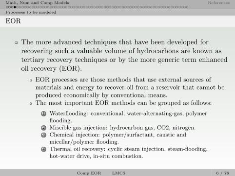
The more advanced techniques that have been developed forrecovering such a valuable volume of hydrocarbons are known astertiary recovery techniques or by the more generic term enhancedoil recovery (EOR).
EOR processes are those methods that use external sources ofmaterials and energy to recover oil from a reservoir that cannot beproduced economically by conventional means.The most important EOR methods can be grouped as follows:
1 Waterflooding: conventional, water-alternating-gas, polymerflooding.
2 Miscible gas injection: hydrocarbon gas, CO2, nitrogen.3 Chemical injection: polymer/surfactant, caustic and
micellar/polymer flooding.4 Thermal oil recovery: cyclic steam injection, steam-flooding,
hot-water drive, in-situ combustion.
Comp EOR LMCS 6 / 76

Math, Num and Comp Models References
Processes to be modeled
EOR
The more advanced techniques that have been developed forrecovering such a valuable volume of hydrocarbons are known astertiary recovery techniques or by the more generic term enhancedoil recovery (EOR).
EOR processes are those methods that use external sources ofmaterials and energy to recover oil from a reservoir that cannot beproduced economically by conventional means.
The most important EOR methods can be grouped as follows:
1 Waterflooding: conventional, water-alternating-gas, polymerflooding.
2 Miscible gas injection: hydrocarbon gas, CO2, nitrogen.3 Chemical injection: polymer/surfactant, caustic and
micellar/polymer flooding.4 Thermal oil recovery: cyclic steam injection, steam-flooding,
hot-water drive, in-situ combustion.
Comp EOR LMCS 6 / 76
Math, Num and Comp Models References
Processes to be modeled
EOR
The more advanced techniques that have been developed forrecovering such a valuable volume of hydrocarbons are known astertiary recovery techniques or by the more generic term enhancedoil recovery (EOR).
EOR processes are those methods that use external sources ofmaterials and energy to recover oil from a reservoir that cannot beproduced economically by conventional means.The most important EOR methods can be grouped as follows:
1 Waterflooding: conventional, water-alternating-gas, polymerflooding.
2 Miscible gas injection: hydrocarbon gas, CO2, nitrogen.3 Chemical injection: polymer/surfactant, caustic and
micellar/polymer flooding.4 Thermal oil recovery: cyclic steam injection, steam-flooding,
hot-water drive, in-situ combustion.
Comp EOR LMCS 6 / 76
Math, Num and Comp Models References
Processes to be modeled
EOR
The more advanced techniques that have been developed forrecovering such a valuable volume of hydrocarbons are known astertiary recovery techniques or by the more generic term enhancedoil recovery (EOR).
EOR processes are those methods that use external sources ofmaterials and energy to recover oil from a reservoir that cannot beproduced economically by conventional means.The most important EOR methods can be grouped as follows:
1 Waterflooding: conventional, water-alternating-gas, polymerflooding.
2 Miscible gas injection: hydrocarbon gas, CO2, nitrogen.
3 Chemical injection: polymer/surfactant, caustic andmicellar/polymer flooding.
4 Thermal oil recovery: cyclic steam injection, steam-flooding,hot-water drive, in-situ combustion.
Comp EOR LMCS 6 / 76

Math, Num and Comp Models References
Processes to be modeled
EOR
The more advanced techniques that have been developed forrecovering such a valuable volume of hydrocarbons are known astertiary recovery techniques or by the more generic term enhancedoil recovery (EOR).
EOR processes are those methods that use external sources ofmaterials and energy to recover oil from a reservoir that cannot beproduced economically by conventional means.The most important EOR methods can be grouped as follows:
1 Waterflooding: conventional, water-alternating-gas, polymerflooding.
2 Miscible gas injection: hydrocarbon gas, CO2, nitrogen.3 Chemical injection: polymer/surfactant, caustic and
micellar/polymer flooding.
4 Thermal oil recovery: cyclic steam injection, steam-flooding,hot-water drive, in-situ combustion.
Comp EOR LMCS 6 / 76
Math, Num and Comp Models References
Processes to be modeled
EOR
The more advanced techniques that have been developed forrecovering such a valuable volume of hydrocarbons are known astertiary recovery techniques or by the more generic term enhancedoil recovery (EOR).
EOR processes are those methods that use external sources ofmaterials and energy to recover oil from a reservoir that cannot beproduced economically by conventional means.The most important EOR methods can be grouped as follows:
1 Waterflooding: conventional, water-alternating-gas, polymerflooding.
2 Miscible gas injection: hydrocarbon gas, CO2, nitrogen.3 Chemical injection: polymer/surfactant, caustic and
micellar/polymer flooding.4 Thermal oil recovery: cyclic steam injection, steam-flooding,
hot-water drive, in-situ combustion.
Comp EOR LMCS 6 / 76
Math, Num and Comp Models References
Reservoir Properties
Table of contents
1 Math, Num and Comp ModelsProcesses to be modeledReservoir PropertiesOne–Phase FlowTwo–Phase Immiscible FlowBlack–OilCompositional OilSolution Schemes
2 References
Comp EOR LMCS 7 / 76

Math, Num and Comp Models References
Reservoir Properties
Petroleum reservoir
Is a subsurface pool of hydrocarbons contained in porous formations.The naturally occurring hydrocarbons, such as crude oil or natural gas,are trapped by overlying rock formations with lower permeability. Italso can contains water, in such a way that in general we have threephases: oleic (o), aqueous (w) and gaseous (g).
Comp EOR LMCS 8 / 76

Math, Num and Comp Models References
Reservoir Properties
Rock: Pores, Porosity and Permeability (Chen [1]) I
Pores: Pores are the tiny connected passages that exists in apermeable rock (≈ 1–200µm).
Porosity: is the fraction of a rock that is pore space. It measuresthe capacity of the reservoir to store productible fluids in its pores.
φ =VpV
φe =VeV
Vp interconnected andisolated pore spaces;Ve interconnected porespaces;V total volume.
Porosity depends on pressure due to rock compressibility: cR = 1φdφdp
φ = φ0ecR(p−p0) =⇒ φ = φ0{
1 + cR(p− p0) +1
2!c2R(p− p0) + . . .
}Comp EOR LMCS 9 / 76
Math, Num and Comp Models References
Reservoir Properties
Rock: Pores, Porosity and Permeability (Chen [1]) II
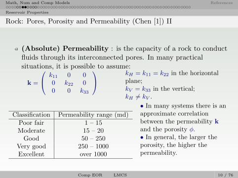
(Absolute) Permeability : is the capacity of a rock to conductfluids through its interconnected pores. In many practicalsituations, it is possible to assume:
k =
k11 0 00 k22 00 0 k33
kH = k11 = k22 in the horizontalplane;kV = k33 in the vertical;kH 6= kV .
Classification Permeability range (md)Poor fair 1 – 15Moderate 15 – 20
Good 50 – 250Very good 250 – 1000Excellent over 1000
• In many systems there is anapproximate correlationbetween the permeability kand the porosity φ.• In general, the larger theporosity, the higher thepermeability.
Comp EOR LMCS 10 / 76

Math, Num and Comp Models References
Reservoir Properties
Fluid: Phase and component (Chen [1])
Phase : refers to a chemically homogeneous region of fluid that isseparated from another phase by an interface, e.g. oleic (o),aqueous (w), gaseous (g), or solid (rock).
Component : is a single chemical species that may be present ina phase, e.g. oleic contains hundreds of components (C1, C2, ...)
Compressibility : of a fluid can be defined in terms of thevolume V or density ρ change with pressure:
cf = − 1
V
∂V
∂p
∣∣∣T
=1
ρ
∂ρ
∂p
∣∣∣T
at a fixed temperature T
ρ = ρ0ecf (p−p0) =⇒ ρ = ρ0
{1 + cf (p− p0) +
1
2!c2f (p− p0) + . . .
}
Comp EOR LMCS 11 / 76

Math, Num and Comp Models References
Reservoir Properties
Rock/Fluid, (Chen [1]) I
Wettability : measures the preference of the rock surface to bewetted by a particular phase.
• Water wet formation is where wateris the preferred wetting phase.
• Oil wet formation is where oil is the
preferred wetting phase.
Fluid saturation : is the fraction of the pore space that a phaseoccupies. For three-phase flow of oil, water and gas, if the threefluids jointly fill the pore space, then the saturations So, Sw andSg satisfy: So + Sw + Sg = 1
Comp EOR LMCS 12 / 76

Math, Num and Comp Models References
Reservoir Properties
Rock/Fluid, (Chen [1]) II
Residual saturation : is the amount of a phase (fraction of porespace) that is trapped or irreducible (Srα, α = w, o, g).
Capillary pressure : In two phase flow, a discontinuity in fluidpressure occurs across an interface between any two immisciblefluids (w − o).
Suppose oil is the non-wetting phase and water is the wetting phase,then the capillary pressure is : pc = po − pw. In general, pc(Sα).For a three phase flow, two capillary pressures are needed:pcow = po − pw and pcgo = pg − po.A third capillary pressure can be obtained as follows :pcgw = pg − pw = pcow + pcgo.Usually is assumed that pcow = pcow(Sw) and pcgo = pcgo(Sg).
Comp EOR LMCS 13 / 76

Math, Num and Comp Models References
Reservoir Properties
Rock/Fluid, (Chen [1]) III
Relative permeability: is a quantity (fraction) that describesthe amount of impairment to flow of one phase on another. Therelative permeabilities to the water, oil, and gas phases are,respectively, denoted by krw, kro, and krg.
Mobility : of a phase is defined as the ratio of the relativepermeability and viscosity of that phase.
The relative permeabilities to the water, oil and gas phases aredenoted λw = krw/µw, λo = kro/µo and λg = krg/µg respectively.The total mobility is the sum of all involved mobilities, for examplein a three-phase flow: λ = λw + λo + λg.
Fractional flow : is a quantity (fraction) that determines thefractional volumetric flow rate of a phase under a given pressuregradient in the presence of another phase. Notation for water, oil,and gas is: fw = λw/λ, fo = λo/λ, fg = λg/λ.
Comp EOR LMCS 14 / 76

Math, Num and Comp Models References
One–Phase Flow
Table of contents
1 Math, Num and Comp ModelsProcesses to be modeledReservoir PropertiesOne–Phase FlowTwo–Phase Immiscible FlowBlack–OilCompositional OilSolution Schemes
2 References
Comp EOR LMCS 15 / 76

Math, Num and Comp Models References
One–Phase Flow
Mathematical models of petroleum reservoirs have been utilizedsince the late 1800s.
A mathematical model consists of a set of equations that describethe flow of fluids in a petroleum reservoir, together with anappropriate set of boundary and/or initial conditions.
Fluid motion in a petroleum reservoir is governed by the
Balance of mass.Balance of momentum.Balance of energy.
In the simulation of flow in the reservoir, the momentum equationis given in the form of Darcy’s law [2].
Derived empirically, this law indicates a linear relationship betweenthe fluid velocity relative to the solid and the pressure headgradient.Its theoretical basis can be revised in, e.g. [3].
Comp EOR LMCS 16 / 76

Math, Num and Comp Models References
One–Phase Flow
The following assumptions are usually adopted:
The porous medium is saturated by the fluid.The mass of the fluid is conserved.
The model is based on only one extensive property:
M(t) ≡∫B(t)
φ(~x, t)ρ(~x, t)d~x.
Then, the basic mathematical model for flow of a fluid through aporous media is
∂(φρ)
∂t+∇ · ~f = q where ~f = φρ~v − ~τ
Comp EOR LMCS 17 / 76

Math, Num and Comp Models References
One–Phase Flow
The velocity ~v is given by the Darcy’s law:
~u = − 1
µk(∇p− ρG∇D) where ~u = φ~v
If we suppose no diffusion, i.e. ~τ = 0 then the general equation forsingle phase flow is:(
φ∂ρ
∂p+ ρ
dφ
dp
)∂p
∂t= ∇ ·
(ρ
µk(∇p− ρG∇D)
)+ q
Equations of state: cR =1
φ
dφ
dpand cf =
1
ρ
∂ρ
∂p
∣∣∣T
For slightly compressible rock we have:
φ ≈ φ0(1 + cR(p− p0)) =⇒ dφ
dp= φ0cR
Comp EOR LMCS 18 / 76

Math, Num and Comp Models References
One–Phase Flow
Finally:
φρct∂p
∂t= ∇ ·
(ρ
µk(∇p− ρG∇D)
)+ q
where ct = cf +φ0
φcR is the total compressibility.
This equation is parabolic in p with ρ given by a state equation(e.g. slightly compressible fluid or ideal gas law).
Boundary conditions:
Dirichlet: the pressure is specified as a known function of positionand time on ∂B the condition is : p = g1 on ∂B.Neumann: the total mass flux is known on ∂B, the boundarycondition is ρ~u · ~n = g2 on ∂B. For impervious boundary g2 = 0Robin: this is a mixed boundary condition and takes the form:gpp+ guρ~u · ~n = g3 on ∂B.
The initial condition can be defined in terms of p:p(~x, 0) = p0(~x), ~x ∈ B.
Comp EOR LMCS 19 / 76

Math, Num and Comp Models References
One–Phase Flow
Simple test
Consider a horizontal domain of length L = 100.
Assume: k = cte, µ = cte, cT = cte, no gravity and no sources.
φµcTk
∂p
∂t=∂2p
∂x2
Boundary conditions: p = 2 on the left, and p = 1 on the right.
Initial condition: p0 = 1.
Input data: φ = 0.2;µ = 1.0; k = 1.0; cT = 10−4
Comp EOR LMCS 20 / 76

Math, Num and Comp Models References
One–Phase Flow
Applying TUNA
StructuredMesh<Uniform<double, 1> > mesh(length, num_nodes);
ScalarField1D p ( mesh.getExtentVolumes() );
DiagonalMatrix< double, 1> A(num_nodes);
ScalarField1D b(num_nodes);
ScalarEquation< CDS<double, 1> > single_phase(p, A, b, mesh.getDeltas());
single_phase.setDeltaTime(dt);
single_phase.setGamma(Gamma);
single_phase.setDirichlet(LEFT_WALL);
single_phase.setDirichlet(RIGHT_WALL);
while (t <= Tmax) {
single_phase.calcCoefficients();
Solver::TDMA1D(single_phase);
error = single_phase.calcErrorL1();
single_phase.update();
t += dt;
}
Comp EOR LMCS 21 / 76

Math, Num and Comp Models References
One–Phase Flow
Result
Comp EOR LMCS 22 / 76

Math, Num and Comp Models References
Two–Phase Immiscible Flow
Table of contents
1 Math, Num and Comp ModelsProcesses to be modeledReservoir PropertiesOne–Phase FlowTwo–Phase Immiscible FlowBlack–OilCompositional OilSolution Schemes
2 References
Comp EOR LMCS 23 / 76

Math, Num and Comp Models References
Two–Phase Immiscible Flow
The following assumptions are usually adopted:
We consider two–phase flow where the fluids are immiscible (o, w).There is no mass transfer between the phases.One phase (w) wets porous medium more than the other (o).The two fluids jointly fill the voids: Sw + So = 1.The pressure in the wetting fluid is less than that in thenon-wetting fluid. The pressure difference is given by the capillarypressure: pc = po − pw. And pc = pc(Sw).There is no diffusion ~τ = 0.
Extensive properties: Mα(t) =
∫B(t)
φραSαd~x, α = w, o.
Intensive properties: ψ = φραSα, α = w, o.
Comp EOR LMCS 24 / 76

Math, Num and Comp Models References
Two–Phase Immiscible Flow
Balance equations:
∂(φραSα)
∂t+∇ · (φραSα~vα) = qα for α = w, o.
Darcy’s Law:
~uα = −krαµα
k(∇pα − ραG∇D) where ~uα = φSα~vα
Recall that:
Sw + So = 1 and pc = po − pw.
We have six equations for six unknowns: ρα, ~uα and Sα, forα = w, o.
Comp EOR LMCS 25 / 76

Math, Num and Comp Models References
Two–Phase Immiscible Flow
Alternative differential equations:
Formulation in phase pressures
Assume: Sw = p−1c (po − pw).
We use pw and po as the main unknowns:
∇ ·(ρwµw
krwk(∇pw − ρwG∇D)
)=∂(φρwp
−1c )
∂t− qw
∇ ·(ρoµokrok(∇po − ρoG∇D)
)=∂(φρo(1− p−1
c ))
∂t− qo
This system is commonly employed in the simultaneos solution (SS)scheme.
Comp EOR LMCS 26 / 76

Math, Num and Comp Models References
Two–Phase Immiscible Flow
Formulation in phase pressure and saturationWe use po and Sw as the main variables:
∇ ·(ρwµw
krwk
(∇po −
dpcdSw∇Sw − ρwG∇D
))=∂(φρwSw)
∂t− qw
1
ρw∇ ·(ρwµw
krwk
(∇po −
dpcdSw∇Sw − ρwG∇D
))+
1
ρo∇ ·(ρoµokrok (∇po − ρoG∇D)
)=
Swρw
∂(φρw)
∂t+
1− Swρo
∂(φρo)
∂t− qwρw− qwρw
Saturation Sw is explicitly evaluated using the first equation. Thesecond equation can be solved for po implicitly. This is the ImplicitPressure Explicit Saturation (IMPES) scheme.
Comp EOR LMCS 27 / 76

Math, Num and Comp Models References
Two–Phase Immiscible Flow
Example: Pressure-Saturation Formulation I
Phases: α = water(w) and oil(o).
Phase mobility functions: λα = krα/µα
Total mobility: λ =∑λα
Fractional flow functions: fα = λα/λ,∑fα = 1
Total velocity: ~u =∑~uα
po ≡ p, Sw ≡ S, pcow ≡ pc(S)
The capillary pressure gradient and permeability are expressed as:
∇pc =dpcdS∇S and k ≡
k11 0 00 k22 00 0 k33
=
k 0 00 k 00 0 k
No gravity: G = 0.
Comp EOR LMCS 28 / 76
Math, Num and Comp Models References
Two–Phase Immiscible Flow
Example: Pressure-Saturation Formulation II
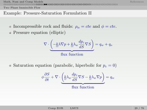
Incompressible rock and fluids: ρα = cte and φ = cte.
Pressure equation (elliptic)
∇ ·(−kλ∇p+ kλw
dpcdS∇S)
︸ ︷︷ ︸flux function
= qw + qo
Saturation equation (parabolic, hiperbolic for pc = 0)
φ∂S
∂t+∇ ·
(kλw
dpcdS∇S − kλw∇p
)︸ ︷︷ ︸
flux function
= qw
Comp EOR LMCS 29 / 76

Math, Num and Comp Models References
Two–Phase Immiscible Flow
FVM: Pressure eq. 1D I
i+ 12∫
i− 12
∇ · (−kλ∇p+ kFw∇S) dx = 0
Fw = λwdpcdS
−
((kλdp
dx
)i+ 1
2
−(kλdp
dx
)i− 1
2
)+
(kFw
dS
dx
)i+ 1
2
−(kFw
dS
dx
)i− 1
2
= 0,
aipi − ai+1pi+1 − ai−1pi−1 − a∗iSi + a∗
i+1Si+1 + a∗i−1Si−1 = 0.
Comp EOR LMCS 30 / 76

Math, Num and Comp Models References
Two–Phase Immiscible Flow
FVM: Pressure eq. 1D II
ai+1 =k
∆x(λ)i+ 1
2; ai−1 =
k
∆x(λ)i− 1
2; ai = ai+1 + ai−1.
a∗i+1 =
k
∆x(Fw)i+ 1
2; a∗
i−1 =k
∆x(Fw)i− 1
2; a∗
i = a∗i+1 + a∗
i−1.
Fw = λwdpcdS
Comp EOR LMCS 31 / 76

Math, Num and Comp Models References
Two–Phase Immiscible Flow
FVM: Saturation eq. 1D I
i+ 12∫
i− 12
n+1∫n
φ∂S
∂tdtdx−
n+1∫n
i+ 12∫
i− 12
∇ ·(kλw∇p− kλw
dpcdSw∇Sw
)dxdt = 0,
φ(Sn+1i − Sni
)∆x−
((kλw
∂p
∂x
)ni+ 1
2
−(kλw
∂p
∂x
)ni− 1
2
)∆t +((
kFw∂S
∂x
)ni+ 1
2
−(kFw
∂S
∂x
)ni− 1
2
)∆t = 0
Sn+1i = Sni + b∗iS
ni − b∗i+1S
ni+1 − b∗i−1S
ni−1 − bip
ni + bi+1p
ni+1 + bi−1p
ni−1.
Comp EOR LMCS 32 / 76

Math, Num and Comp Models References
Two–Phase Immiscible Flow
FVM: Saturation eq. 1D II
bi+1 =k∆t
φ∆x2(λw)ni+ 1
2; bi−1 =
k∆t
φ∆x2(λw)ni− 1
2; bi = bi+1 + bi−1; .
b∗i+1 =k∆t
φ∆x2(Fw)ni+ 1
2; b∗i−1 =
k∆t
φ∆x2(Fw)ni− 1
2; b∗i = b∗i+1 + b∗i−1.
Fw = λwdpcdS
Comp EOR LMCS 33 / 76

Math, Num and Comp Models References
Two–Phase Immiscible Flow
FVM: IMPES
The coefficients are not constant and depend on λ, λw and Fw:
(λ)ni± 1
2
, (λw)ni± 1
2
, (Fw)ni± 1
2
Fw = λwdpc
dS
IMPES Algorithm
1: while (t < Tmax) do2: Calc. coeff. of pressure equation.3: Solve the pressure equation implicitly.4: Calc. coeff. of saturation equation.5: Solve the saturation eq. explicitly.6: t← t+ ∆t7: end while
while ( t <= Tmax) {pre s su r e . c a l c C o e f f i c i e n t s ( ) ;So lve r : :TDMA1D( pr e s su r e ) ;p r e s su r e . update ( ) ;
s a t u r a t i o n . c a l c C o e f f i c i e n t s ( ) ;So lve r : : s o l E x p l i c i t ( s a t u r a t i o n ) ;s a t u r a t i o n . update ( ) ;
t += dt ;}
Comp EOR LMCS 34 / 76

Math, Num and Comp Models References
Two–Phase Immiscible Flow
Inheritance I
General Equation:
Conservative form:∂
∂t
∫B(t)
ψd~x+
∫B(t)
∇ · ~fd~x =
∫B(t)
qd~x
Discrete general equation:an+1P
ψn+1P
=
an+1e
ψn+1e
+an+1w
ψn+1w
+an+1n
ψn+1n
+an+1s
ψn+1s
+an+1f
ψn+1f
+an+1b
ψn+1b
+qnP
Two phase immiscible and incompressible fluids:
Pressure and saturation equations are derived from generalequation:
∇ ·(−kλ∇p+ kλw
dpc
dS∇S)
= qw + qo
φ∂S
∂t+∇ ·
(kλw
dpc
dS∇S − kλw∇p
)= qw
Comp EOR LMCS 35 / 76

Math, Num and Comp Models References
Two–Phase Immiscible Flow
Inheritance II
Inheritance is a way to share and reuse code by defining collectionsof attributes and behaviors, bundled into classes (subclasses),based on previously created classes (superclasses).
Inheritance gives rise to hierarchies: complexity is reduced, butefficiency can be spoiled.
Comp EOR LMCS 36 / 76

Math, Num and Comp Models References
Two–Phase Immiscible Flow
Object declaration
Pressure
TwoPhaseEquation< BLIP1<double , 1> > pre s su r e (p , A, b , mesh . ge tDe l ta s ( ) ) ;p r e s su r e . setDeltaTime ( dt ) ;p r e s su r e . s e tPe rmeab i l i t y ( pe rmeab i l i ty ) ;p r e s su r e . s e tPo ro s i t y ( po ro s i t y ) ;p r e s su r e . setSrw (Srw ) ;p r e s su r e . s e tSro ( Sro ) ;p r e s su r e . s e tV i s c o s i t y w (mu w ) ;p r e s su r e . s e t V i s c o s i t y o (mu o ) ;p r e s su r e . setNeumann (LEFT WALL, i n j e c t i o n ) ;p r e s su r e . s e t D i r i c h l e t (RIGHT WALL) ;p r e s su r e . s e tSa tu ra t i on (Sw ) ;p r e s su r e . p r i n t ( ) ;
Saturation
TwoPhaseEquation< BLES1<double , 1> > s a tu ra t i on (Sw, A, b , mesh . ge tDe l ta s ( ) ) ;s a tu ra t i on . setDeltaTime ( dt ) ;s a tu ra t i on . s e tPe rmeab i l i t y ( pe rmeab i l i ty ) ;s a tu ra t i on . s e tPo ro s i t y ( po ro s i t y ) ;s a tu ra t i on . setSrw (Srw ) ;s a tu ra t i on . s e tSro ( Sro ) ;s a tu ra t i on . s e tV i s c o s i t y w (mu w ) ;s a tu ra t i on . applyBounds (1 , Sw . ubound ( f i r s tDim ) −1);s a tu ra t i on . s e tPr e s su r e (p ) ;s a tu ra t i on . p r in t ( ) ;
Comp EOR LMCS 37 / 76

Math, Num and Comp Models References
Two–Phase Immiscible Flow
Test 1: Buckley–Leverett (in collaboration with M. Diaz [7])
From Diaz et al. [7]Property Value
Length 300 m
k 1.0E-15 m2
φ 0.2
µw 1.0E-03 Pa.s
µo 1.0E-03 Pa.s
Srw 0
Sro 0.2
ginp 3.4722E-07 m.s−1
pout 1E+07 Pa
Zero capillary pressure
Pressure eq.
−∇ ·(kλ∇p
)= 0
Saturation eq.
φ∂S
∂t−∇ ·
(kλw∇p
)= 0.
Comp EOR LMCS 38 / 76

Math, Num and Comp Models References
Two–Phase Immiscible Flow
Test 1: Buckley–Leverett I
Constitutive Eqs.
krw = Sωe ; kro = (1− Se)ω, ω = 1, 2
Se =S − Srw
1− Srw − Sro
Coefficients:
(λ)i± 12
=1
(1− Srw − Sro)ω
(Si± 1
2− Srw)ω
µw+
(1− Sro − Si± 12)ω
µo
)
(λw)ni± 12
=1
µw
(Sni± 1
2− Srw
1− Srw − Sro
)ω
Comp EOR LMCS 39 / 76

Math, Num and Comp Models References
Two–Phase Immiscible Flow
Test 1: Buckley–Leverett II
Upwind scheme for Si± 12.
if ( pni+1 >= pni ) thenSi+ 1
2= Si+1
elseSi+ 1
2= Si
end if
Comp EOR LMCS 40 / 76

Math, Num and Comp Models References
Two–Phase Immiscible Flow
Test 1: Buckley–Leverett III
Adaptors: BLIP1 & BLES1
template<typename Tprec, int Dim>
class BLIP1 : public TwoPhaseEquation<BLIP1<Tprec, Dim> > {
public:
inline void calcCoefficients1D();
inline void calcCoefficients2D();
inline void calcCoefficients3D();
};
template<typename Tprec, int Dim>
inline void BLIP1<Tprec, Dim>::calcCoefficients1D () {
static prec_t Sw_e, Sw_w;
static prec_t mult_o = k / ( (1 - Srw - Sro) * mu_o * dx ) ;
static prec_t mult_w = k / ( (1 - Srw - Sro) * mu_w * dx ) ;
aE = 0.0; aW = 0.0; aP = 0.0; sp = 0.0;
for (int i = bi; i <= ei; ++i) {
if ( phi_0(i+1) >= phi_0(i) ) Sw_e = S(i+1);
else Sw_e = S(i);
if ( phi_0(i-1) >= phi_0(i) ) Sw_w = S(i-1);
else Sw_w = S(i);
aE (i) = (1 - Sro - Sw_e) * mult_o + (Sw_e - Srw) * mult_w ;
aW (i) = (1 - Sro - Sw_w) * mult_o + (Sw_w - Srw) * mult_w ;
aP (i) = aE (i) + aW (i);
}
applyBoundaryConditions1D();
}
Comp EOR LMCS 41 / 76

Math, Num and Comp Models References
Two–Phase Immiscible Flow
Test 1: Buckley–Leverett IV
template<typename Tprec, int Dim>
class BLES1 : public TwoPhaseEquation<BLES1<Tprec, Dim> >
{
public:
inline void calcCoefficients1D();
inline void calcCoefficients2D();
inline void calcCoefficients3D();
};
template<typename Tprec, int Dim>
inline void BLES1<Tprec, Dim>::calcCoefficients1D ()
{
static prec_t Sw_e, Sw_w;
static prec_t mult = k * dt / ( porosity * dx * dx * (1 - Srw - Sro) * mu_w );
aE = 0.0; aW = 0.0; aP = 0.0; sp = 0.0;
for (int i = bi; i <= ei; ++i) {
if ( phi_0(i+1) >= phi_0(i) ) Sw_e = phi_0(i+1);
else Sw_e = phi_0(i);
if ( phi_0(i-1) >= phi_0(i) ) Sw_w = phi_0(i-1);
else Sw_w = phi_0(i);
aE (i) = (Sw_e - Srw) * mult;
aW (i) = (Sw_w - Srw) * mult;
aP (i) = aE (i) + aW (i);
}
Comp EOR LMCS 42 / 76

Math, Num and Comp Models References
Two–Phase Immiscible Flow
Test 1: Buckley–Leverett V
// Dirichlet right side
aP(ei) += aE(ei);
sp(ei) = 2 * aE(ei) * p(ei+1);
aE(ei) = 0;
// Neumann left side
aP(bi) -= aW(bi) ;
sp(bi) = aW(bi) * dx * ( 3.47e-7 * mu_w / k) ;
aW(bi) = 0;
}
2D rectangular mesh: 300 × 10
Time steps = 1100 days and ∆t = 60 secs. (1,584,000 steps)
Cases:
1 ω = 1 and µw/µo = 1 (lineal01)2 ω = 1 and µw/µo = 2 (lineal02)3 ω = 1 and µw/µo = 2/3 (lineal2 3)4 ω = 2 and µw/µo = 2/3 (quadratic2 3)
Comp EOR LMCS 43 / 76

Math, Num and Comp Models References
Two–Phase Immiscible Flow
Improved IMPES
As described in Chen et al. [8] the improved IMPES consists in to take abigger time step for the calculation of pressure.
∆tp/∆tS SPp SPT1 1.0 1.005 4.7 2.5010 9.6 3.19
Comp EOR LMCS 44 / 76

Math, Num and Comp Models References
Two–Phase Immiscible Flow
Overlapping method I
Comp EOR LMCS 45 / 76

Math, Num and Comp Models References
Two–Phase Immiscible Flow
Overlapping method II
CartComm<2> cart(argc, argv, rank); // MPI::COMM_WORLD.Create_cart()
Isub = cart.get_I();
Jsub = cart.get_J();
num_subdom_x = cart.getNumProc_I();
num_subdom_y = cart.getNumProc_J();
SubDomain<double, 2> subdom(cart);
double ovlp_l = subdom.createOverlap(LEFT, nc_ovlp_l, dx);
double ovlp_r = subdom.createOverlap(RIGHT, nc_ovlp_r, dx);
double ovlp_d = subdom.createOverlap(DOWN, nc_ovlp_d, dy);
double ovlp_u = subdom.createOverlap(UP, nc_ovlp_u, dy);
while (t <= Tmax) { // IMPES loop
//...
subdom.infoExchange1(p);
pressure.updatePhi(p);
subdom.infoExchange1(Sw);
saturation.updatePhi(Sw);
}
Comp EOR LMCS 46 / 76

Math, Num and Comp Models References
Two–Phase Immiscible Flow
Overlapping method III
Results on a Quadcore computer.
Procs. Subdom CPU timep CPU timeS Speed up Eff.
1 1 614.51 170.09 – –2 2 × 1 351.45 155.32 1.55 0.75
4 (1) 4 × 1 165.61 42.79 3.76 0.944 (2) 1 × 4 322.26 76.07 1.97 0.494 (3) 2 × 2 218.45 57.48 2.84 0.71
Comp EOR LMCS 47 / 76

Math, Num and Comp Models References
Two–Phase Immiscible Flow
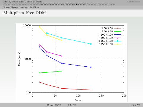
Multipliers–Free DDM
Non–overlapping DDM : Unified theory of multipliers–free DDMmethods, Herrera and Yates [9, 10]
Elliptic Operator – Subdomains = 32 × 32 = 10241
Nx × Ny 50 × 50 100 × 100 150 × 1502,560,000 10,240,000 23,040,000
Proc. K2 P3 K P K P
16 (64) 204 389 2303 2670 – 915832 (32) 172 401 1274 1641 5937 517864 (16) 133 436 745 1234 4326 3647128 (8) 119 – 568 – 2818 –
1Recently results from A. Carrillo and R. Yates2K ≡ KanBalam 1360 AMD Opteron 2.6 GHz, 8 GB per 4 cores, Net 10 Gbps3P ≡ Pohualli 100 Intel Xeon 2.33 GHz, 32 GB per 8 cores, Net 1 Gbps
Comp EOR LMCS 48 / 76
Math, Num and Comp Models References
Two–Phase Immiscible Flow
Multipliers–Free DDM
Comp EOR LMCS 49 / 76

Math, Num and Comp Models References
Two–Phase Immiscible Flow
Test 2: Five–spots
Classical five-spots pattern.
Four water injection wells: awell in each corner of thedomain.
One oil production well: in thecenter of the domain.
Only one quarter of thedomain is simulated.
No flux on the boundaries.
Comp EOR LMCS 50 / 76
Math, Num and Comp Models References
Black–Oil
Table of contents
1 Math, Num and Comp ModelsProcesses to be modeledReservoir PropertiesOne–Phase FlowTwo–Phase Immiscible FlowBlack–OilCompositional OilSolution Schemes
2 References
Comp EOR LMCS 51 / 76

Math, Num and Comp Models References
Black–Oil
The basic hypotheses of the black-oil model are, see [11]:
1 There are three fluid phases in the reservoir: w, o, and g.
2 Solubility of hydrocarbons in the water phase is negligible.3 The water and gas phases only contain one component.4 The oil and water components are not allowed to vaporize into the
gas phase.5 The gas component is allowed to dissolve into the oil phase.6 The oil-phase contains dissolved gas and non-volatile oil.7 Mass diffusive-processes are neglected.8 The system is in thermal equilibrium.9 There is no chemical reactions.10 Three components: W = water component, O = liquid hydrocarbon
component, G = gaseous hydrocarbon component.11 Water phase: wetting phase, Oil phase: intermediate wetting phase,
Gas phase: non-wetting phase.
Comp EOR LMCS 52 / 76

Math, Num and Comp Models References
Black–Oil
The basic hypotheses of the black-oil model are, see [11]:
1 There are three fluid phases in the reservoir: w, o, and g.2 Solubility of hydrocarbons in the water phase is negligible.
3 The water and gas phases only contain one component.4 The oil and water components are not allowed to vaporize into the
gas phase.5 The gas component is allowed to dissolve into the oil phase.6 The oil-phase contains dissolved gas and non-volatile oil.7 Mass diffusive-processes are neglected.8 The system is in thermal equilibrium.9 There is no chemical reactions.10 Three components: W = water component, O = liquid hydrocarbon
component, G = gaseous hydrocarbon component.11 Water phase: wetting phase, Oil phase: intermediate wetting phase,
Gas phase: non-wetting phase.
Comp EOR LMCS 52 / 76

Math, Num and Comp Models References
Black–Oil
The basic hypotheses of the black-oil model are, see [11]:
1 There are three fluid phases in the reservoir: w, o, and g.2 Solubility of hydrocarbons in the water phase is negligible.3 The water and gas phases only contain one component.
4 The oil and water components are not allowed to vaporize into thegas phase.
5 The gas component is allowed to dissolve into the oil phase.6 The oil-phase contains dissolved gas and non-volatile oil.7 Mass diffusive-processes are neglected.8 The system is in thermal equilibrium.9 There is no chemical reactions.10 Three components: W = water component, O = liquid hydrocarbon
component, G = gaseous hydrocarbon component.11 Water phase: wetting phase, Oil phase: intermediate wetting phase,
Gas phase: non-wetting phase.
Comp EOR LMCS 52 / 76

Math, Num and Comp Models References
Black–Oil
The basic hypotheses of the black-oil model are, see [11]:
1 There are three fluid phases in the reservoir: w, o, and g.2 Solubility of hydrocarbons in the water phase is negligible.3 The water and gas phases only contain one component.4 The oil and water components are not allowed to vaporize into the
gas phase.
5 The gas component is allowed to dissolve into the oil phase.6 The oil-phase contains dissolved gas and non-volatile oil.7 Mass diffusive-processes are neglected.8 The system is in thermal equilibrium.9 There is no chemical reactions.10 Three components: W = water component, O = liquid hydrocarbon
component, G = gaseous hydrocarbon component.11 Water phase: wetting phase, Oil phase: intermediate wetting phase,
Gas phase: non-wetting phase.
Comp EOR LMCS 52 / 76

Math, Num and Comp Models References
Black–Oil
The basic hypotheses of the black-oil model are, see [11]:
1 There are three fluid phases in the reservoir: w, o, and g.2 Solubility of hydrocarbons in the water phase is negligible.3 The water and gas phases only contain one component.4 The oil and water components are not allowed to vaporize into the
gas phase.5 The gas component is allowed to dissolve into the oil phase.
6 The oil-phase contains dissolved gas and non-volatile oil.7 Mass diffusive-processes are neglected.8 The system is in thermal equilibrium.9 There is no chemical reactions.10 Three components: W = water component, O = liquid hydrocarbon
component, G = gaseous hydrocarbon component.11 Water phase: wetting phase, Oil phase: intermediate wetting phase,
Gas phase: non-wetting phase.
Comp EOR LMCS 52 / 76

Math, Num and Comp Models References
Black–Oil
The basic hypotheses of the black-oil model are, see [11]:
1 There are three fluid phases in the reservoir: w, o, and g.2 Solubility of hydrocarbons in the water phase is negligible.3 The water and gas phases only contain one component.4 The oil and water components are not allowed to vaporize into the
gas phase.5 The gas component is allowed to dissolve into the oil phase.6 The oil-phase contains dissolved gas and non-volatile oil.
7 Mass diffusive-processes are neglected.8 The system is in thermal equilibrium.9 There is no chemical reactions.10 Three components: W = water component, O = liquid hydrocarbon
component, G = gaseous hydrocarbon component.11 Water phase: wetting phase, Oil phase: intermediate wetting phase,
Gas phase: non-wetting phase.
Comp EOR LMCS 52 / 76

Math, Num and Comp Models References
Black–Oil
The basic hypotheses of the black-oil model are, see [11]:
1 There are three fluid phases in the reservoir: w, o, and g.2 Solubility of hydrocarbons in the water phase is negligible.3 The water and gas phases only contain one component.4 The oil and water components are not allowed to vaporize into the
gas phase.5 The gas component is allowed to dissolve into the oil phase.6 The oil-phase contains dissolved gas and non-volatile oil.7 Mass diffusive-processes are neglected.
8 The system is in thermal equilibrium.9 There is no chemical reactions.10 Three components: W = water component, O = liquid hydrocarbon
component, G = gaseous hydrocarbon component.11 Water phase: wetting phase, Oil phase: intermediate wetting phase,
Gas phase: non-wetting phase.
Comp EOR LMCS 52 / 76

Math, Num and Comp Models References
Black–Oil
The basic hypotheses of the black-oil model are, see [11]:
1 There are three fluid phases in the reservoir: w, o, and g.2 Solubility of hydrocarbons in the water phase is negligible.3 The water and gas phases only contain one component.4 The oil and water components are not allowed to vaporize into the
gas phase.5 The gas component is allowed to dissolve into the oil phase.6 The oil-phase contains dissolved gas and non-volatile oil.7 Mass diffusive-processes are neglected.8 The system is in thermal equilibrium.
9 There is no chemical reactions.10 Three components: W = water component, O = liquid hydrocarbon
component, G = gaseous hydrocarbon component.11 Water phase: wetting phase, Oil phase: intermediate wetting phase,
Gas phase: non-wetting phase.
Comp EOR LMCS 52 / 76

Math, Num and Comp Models References
Black–Oil
The basic hypotheses of the black-oil model are, see [11]:
1 There are three fluid phases in the reservoir: w, o, and g.2 Solubility of hydrocarbons in the water phase is negligible.3 The water and gas phases only contain one component.4 The oil and water components are not allowed to vaporize into the
gas phase.5 The gas component is allowed to dissolve into the oil phase.6 The oil-phase contains dissolved gas and non-volatile oil.7 Mass diffusive-processes are neglected.8 The system is in thermal equilibrium.9 There is no chemical reactions.
10 Three components: W = water component, O = liquid hydrocarboncomponent, G = gaseous hydrocarbon component.
11 Water phase: wetting phase, Oil phase: intermediate wetting phase,Gas phase: non-wetting phase.
Comp EOR LMCS 52 / 76

Math, Num and Comp Models References
Black–Oil
The basic hypotheses of the black-oil model are, see [11]:
1 There are three fluid phases in the reservoir: w, o, and g.2 Solubility of hydrocarbons in the water phase is negligible.3 The water and gas phases only contain one component.4 The oil and water components are not allowed to vaporize into the
gas phase.5 The gas component is allowed to dissolve into the oil phase.6 The oil-phase contains dissolved gas and non-volatile oil.7 Mass diffusive-processes are neglected.8 The system is in thermal equilibrium.9 There is no chemical reactions.10 Three components: W = water component, O = liquid hydrocarbon
component, G = gaseous hydrocarbon component.
11 Water phase: wetting phase, Oil phase: intermediate wetting phase,Gas phase: non-wetting phase.
Comp EOR LMCS 52 / 76

Math, Num and Comp Models References
Black–Oil
The basic hypotheses of the black-oil model are, see [11]:
1 There are three fluid phases in the reservoir: w, o, and g.2 Solubility of hydrocarbons in the water phase is negligible.3 The water and gas phases only contain one component.4 The oil and water components are not allowed to vaporize into the
gas phase.5 The gas component is allowed to dissolve into the oil phase.6 The oil-phase contains dissolved gas and non-volatile oil.7 Mass diffusive-processes are neglected.8 The system is in thermal equilibrium.9 There is no chemical reactions.10 Three components: W = water component, O = liquid hydrocarbon
component, G = gaseous hydrocarbon component.11 Water phase: wetting phase, Oil phase: intermediate wetting phase,
Gas phase: non-wetting phase.
Comp EOR LMCS 52 / 76

Math, Num and Comp Models References
Black–Oil
PhasesComponent Aqueos (w) Oleic (o) Gaseous (g)
W φρwSw (ρWw ≡ ρw)O φρOoSwG φρGoSo φρgSg (ρGg ≡ ρg)
(dg) (fg)dg : dissolved gas; fg : free gas.
Balance equations:
Water component:∂(φρwSw)
∂t= −∇ · (ρw~uw) + qW
Oil component:∂(φρOoSo)
∂t= −∇ · (ρOo~uo) + qO
Gas component:
∂(
dg︷ ︸︸ ︷φρGoSo +
fg︷ ︸︸ ︷φρgSg))
∂t= −∇ · ( ρGo~uo︸ ︷︷ ︸
flow dg
+
flow fg︷ ︸︸ ︷ρg~ug ) + qG
Comp EOR LMCS 53 / 76

Math, Num and Comp Models References
Black–Oil
Darcy’s Law:
~uw = −krwµw
k(∇pw − ρwG∇D)
~uo = −kroµo
k(∇po − ρoG∇D) (where ρo = ρOo + ρGo)
~ug = −krgµg
k(∇pg − ρgG∇D)
Saturation constrain: Sw + So + Sg = 1.Capillary pressures: pcgw = pg − pw; pcow = po − pw; pcgo = pg − po.
We have: 3 mass conservation eqs, 3 Darcy’s Law eqs, 1 sat.constrain, 2 capillary pressure. Total: 9 eqs.
We have 9 unknowns: pw, po, pg, ~uw, ~uo, ~ug, Sw, So, and Sg.
Comp EOR LMCS 54 / 76

Math, Num and Comp Models References
Black–Oil
Pressure–Saturation Formulation for Black–Oil Model
Pressure equation (oil)
cT∂p
∂t+∇ · u =
∑α
1
ρα
{qα − ρ0
αcαuα · ∇p}, α = w, o, g,
Saturation equation (water and gas)
ραφ∂sα∂t
+ ρα∇ · uα = −(sαραφ0cp + φsαρ
0αcα)
∂p
∂t−ρ0
αcαuα · ∇p+ qα, α = w, g.
Comp EOR LMCS 55 / 76
Math, Num and Comp Models References
Black–Oil
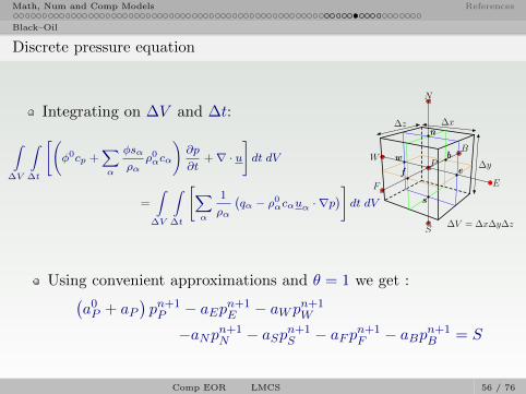
Discrete pressure equation
Integrating on ∆V and ∆t:
∫∆V
∫∆t
[(φ0cp +
∑α
φsα
ραρ0αcα
)∂p
∂t+∇ · u
]dt dV
=
∫∆V
∫∆t
[∑α
1
ρα
(qα − ρ0
αcαuα · ∇p)]dt dV
∆x∆z
∆y
E
W
N
S
F
B
Pee
ww
nn
ss
ff
bb
∆V = ∆x∆y∆z
Using convenient approximations and θ = 1 we get :(a0P + aP
)pn+1P − aEpn+1
E − aW pn+1W
−aNpn+1N − aSpn+1
S − aF pn+1F − aBpn+1
B = S
Comp EOR LMCS 56 / 76
Math, Num and Comp Models References
Black–Oil
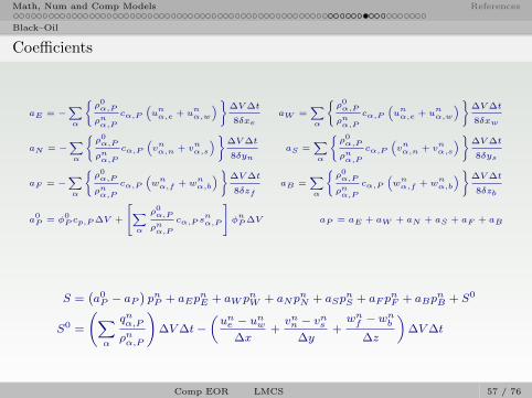
Coefficients
aE = −∑α
{ρ0α,P
ρnα,P
cα,P
(unα,e + u
nα,w
)}∆V∆t
8δxeaW =
∑α
{ρ0α,P
ρnα,P
cα,P
(unα,e + u
nα,w
)}∆V∆t
8δxw
aN = −∑α
{ρ0α,P
ρnα,P
cα,P
(vnα,n + v
nα,s
)}∆V∆t
8δynaS =
∑α
{ρ0α,P
ρnα,P
cα,P
(vnα,n + v
nα,s
)}∆V∆t
8δys
aF = −∑α
{ρ0α,P
ρnα,P
cα,P
(wnα,f + w
nα,b
)}∆V∆t
8δzfaB =
∑α
{ρ0α,P
ρnα,P
cα,P
(wnα,f + w
nα,b
)}∆V∆t
8δzb
a0P = φ
0P cp,P∆V +
∑α
ρ0α,P
ρnα,P
cα,P snα,P
φnP∆V aP = aE + aW + aN + aS + aF + aB
S =(a0P − aP
)pnP + aEp
nE + aW pnW + aNp
nN + aSp
nS + aF p
nF + aBp
nB + S0
S0 =
(∑α
qnα,P
ρnα,P
)∆V∆t−
(une − unw
∆x+vnn − vns
∆y+wnf − w
nb
∆z
)∆V∆t
Comp EOR LMCS 57 / 76
Math, Num and Comp Models References
Black–Oil
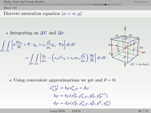
Discrete saturation equation (α = w, g)
Integrating on ∆V and ∆t:∫∆V
∫∆t
[φ∂sα∂t
+∇ · uα + cαρ0α
ραuα · ∇p
]dt dV
=
∫∆V
∫∆t
[qαρα−(sαφ
0cp + sαφcαρ0α
ρα
)∂p
∂t
]dt dV
∆x∆z
∆y
E
W
N
S
F
B
Pee
ww
nn
ss
ff
bb
∆V = ∆x∆y∆z
Using convenient approximations we get and θ = 0:
sn+1α,P = bP s
nα,P + dP
bP = bP (φnP , ρnα,P , p
nP , p
n+1P )
dP = dP (φnP , ρnα,P , q
nP , p
n, unα)
Comp EOR LMCS 58 / 76

Math, Num and Comp Models References
Black–Oil
Explicit equation for saturation (α = w, g)
sn+1α,P =snα,P − snα,P
[cp,P
φ0P
φnP+ cα,P
ρ0α,P
ρnα,P
] (pn+1P − pnP
)+
qnα,Pρnα,Pφ
nP
∆t
− ∆t
φnP
[unα,e − unα,w
∆x+vnα,n − vnα,s
∆y+wnα,f − wnα,b
∆z
]−ρ0α,P cα,P
ρnα,PφnP
∆t
[unα,e + unα,w
4
(pnE − pnPδxe
−pnW − pnPδxw
)+
vnα,n + vnα,s4
(pnN − pnPδyn
−pnS − pnPδys
)+
wnα,f + wnα,b4
(pnF − pnPδzf
−pnB − pnPδzb
)]
Comp EOR LMCS 59 / 76

Math, Num and Comp Models References
Black–Oil
Solution Algorithm
Comp EOR LMCS 60 / 76

Math, Num and Comp Models References
Compositional Oil
Table of contents
1 Math, Num and Comp ModelsProcesses to be modeledReservoir PropertiesOne–Phase FlowTwo–Phase Immiscible FlowBlack–OilCompositional OilSolution Schemes
2 References
Comp EOR LMCS 61 / 76

Math, Num and Comp Models References
Compositional Oil
Assumptions:
Compositional flow involves many components and mass transferbetween phases in a general fashion.The flow process is isothermal.The components form at most three phases.There is no mass transfer between the water phase and thehydrocarbon phases.
Total mass is conserved for each component:
Water component:
(φξwSw)
∂t+∇ · (ξw~uw) = qw
where ξw is the molar density of the water.
Comp EOR LMCS 62 / 76

Math, Num and Comp Models References
Compositional Oil
Hydrocarbon components:
φ(xioξoSo + xigξgSg)
∂t+∇ · (xioξo~uo + xigξg~ug)+
∇ · (dio
+ dig
) = qi, i = 1, . . . , Nc
where ξio, xiα and diα
represents the molar densities, the molefraction, and the difussive fluxes of componet i in the phase α,respectively. α = o, g. Nc is the number of hydrocarboncomponents,
Darcy’s Law:
~uα = −krαµα
k(∇pα − ραG∇D) for α = w, o, g.
Comp EOR LMCS 63 / 76

Math, Num and Comp Models References
Compositional Oil
The mole fraction balance implies:
Nc∑i=1
xio = 1 and
Nc∑i=1
xig = 1
Saturation constrain: Sw + So + Sg = 1.
Capillary pressures: pcow = po − pw; pcgo = pg − po.We have Nc + 9 equations and 2Nc + 9 unknowns: xio, xig, ~uα, ραand Sα, for α = w, o, g and i = 1, . . . , Nc.
The aditional Nc relations are provided by the equilibriumrelations that relate the numbers of moles:
fio(po, x1o, . . . xNco) = fig(pg, x1g, . . . xNcg)
Typical (moderate) simulation: grid nodes ∼ 105 andNc = 10 =⇒∼ 3× 10⁶ unknowns by time step.
Comp EOR LMCS 64 / 76

Math, Num and Comp Models References
Solution Schemes
Table of contents
1 Math, Num and Comp ModelsProcesses to be modeledReservoir PropertiesOne–Phase FlowTwo–Phase Immiscible FlowBlack–OilCompositional OilSolution Schemes
2 References
Comp EOR LMCS 65 / 76

Math, Num and Comp Models References
Solution Schemes
Solution Schemes I
An important problem in the numerical simulation is to developstable, efficient, robust, accurate, and self-adaptive time steppingtechniques.
IMPES method.
This scheme works well for problems of intermediate difficulty andnonlinearity (e.g., for two-phase incompressible flow) and is stillwidely used in the petroleum industry.However, it is not efficient for problems with strong nonlinearities,particularly for problems involving more than two fluid phases.
Simultaneous solution (SS) method.
Solves all of the coupled nonlinear equations simultaneously andimplicitly.This technique is stable and can take very large time steps whilestability is maintained.
Comp EOR LMCS 66 / 76

Math, Num and Comp Models References
Solution Schemes
Solution Schemes II
For the black oil and thermal models (with a few components) is agood choice.However, for complex problems that involve many chemicalcomponents (e.g., the compositional and chemical compositionalflow problems), the size of system matrices to be solved is too large.
Sequential methods, implicit fashion without a full coupling.
They are less stable but more computationally efficient than the SSscheme, and more stable but less efficient than the IMPES scheme.The sequential schemes are very suitable for the compositional andchemical compositional flow problems that involve many chemicalcomponents.
Adaptive implicit scheme can be employed in reservoir simulation.
Comp EOR LMCS 67 / 76

Math, Num and Comp Models References
References I
[1] Z. Chen,Reservoir Simulation: Mathematical Techniques in Oil Recovery,SIAM, 2007.
[2] H. Darcy,Les Fontaines Publiques de la Ville de Dijon,Victor Dalmond, Paris, 1856.
[3] J. Bear,Dynamics of Fluids in Porous Media,Dover, NewYork, 1972.
[4] I. Herrera and M. B. Allen and G. F. Pinder,Numerical modeling in science and engineering,John Wiley & Sons., USA, 1988.
Comp EOR LMCS 68 / 76

Math, Num and Comp Models References
References II
[5] I. Herrera and G. F. Pinder,General principles of mathematical computational modeling,John Wiley, in press.
[6] R.J. LevequeFinite Volume Method for Hyperbolic Problems,Cambridge University Press, 2004.
[7] M.A. Dıaz-Viera and D.A. Lopez-Falcon and A.Moctezuma-Berthier, A. ortiz-Tapia,COMSOL Implementations of Multiphase Fluid Flow Model inPorous Media,COMSOL Conference, Boston, October, 2008.
Comp EOR LMCS 69 / 76

Math, Num and Comp Models References
References III
[8] Z. Chen and G. Huan and Y. Ma,Computational Methods for Multiphase Flows in Poros Media,SIAM, 2006.
[9] I. Herrera and R. Yates,The Multipliers–Free Domain Decomposition Methods,Num. Meth. Part. Diff. Eq., 26, 2010, 874–905.
[10] I. Herrera and R. Yates,Multipliers–Free Dual–Primal Domain Decomposition Methods forNonsymmetric Matrices and Their Numerical TestingNum. Meth. Part. Diff. Eq., Apr. 2010.
[11] K. Aziz and A. Settari,Petroleum Reservoir Simulation,Applied Science Publishers, London, 1979.
Comp EOR LMCS 70 / 76