computational methods in drug discovery - beilstein … · computational methods in drug discovery...

2694

Computational methods in drug discoverySumudu P. Leelananda and Steffen Lindert*

Review Open Access

Address:Department of Chemistry and Biochemistry, Ohio State University,Columbus, OH 43210, USA

Email:Steffen Lindert* - [email protected]

* Corresponding author

Keywords:ADME; computer-aided drug design; docking; free energy;high-throughput screening; LBDD; lead optimization; machinelearning; pharmacophore; QSAR; SBDD; scoring; target flexibility

Beilstein J. Org. Chem. 2016, 12, 2694–2718.doi:10.3762/bjoc.12.267

Received: 01 September 2016Accepted: 22 November 2016Published: 12 December 2016

This article is part of the Thematic Series "Chemical biology".

Guest Editor: H. B. Bode

© 2016 Leelananda and Lindert; licensee Beilstein-Institut.License and terms: see end of document.

AbstractThe process for drug discovery and development is challenging, time consuming and expensive. Computer-aided drug discovery

(CADD) tools can act as a virtual shortcut, assisting in the expedition of this long process and potentially reducing the cost of

research and development. Today CADD has become an effective and indispensable tool in therapeutic development. The human

genome project has made available a substantial amount of sequence data that can be used in various drug discovery projects. Addi-

tionally, increasing knowledge of biological structures, as well as increasing computer power have made it possible to use computa-

tional methods effectively in various phases of the drug discovery and development pipeline. The importance of in silico tools is

greater than ever before and has advanced pharmaceutical research. Here we present an overview of computational methods used in

different facets of drug discovery and highlight some of the recent successes. In this review, both structure-based and ligand-based

drug discovery methods are discussed. Advances in virtual high-throughput screening, protein structure prediction methods, pro-

tein–ligand docking, pharmacophore modeling and QSAR techniques are reviewed.

2694

IntroductionBringing a pharmaceutical drug to the market is a long term

process that costs billions of dollars. In 2014, the Tufts Center

for the Study of Drug Development estimated that the cost asso-

ciated with developing and bringing a drug to the market has in-

creased nearly 150% in the last decade. The cost is now esti-

mated to be a staggering $2.6 billion dollars. The probability of

a failure in the drug discovery and development pipeline is high

and 90% of the drugs entering clinical trials fail to get FDA

approval and reach the consumer market. Approximately 75%

of the cost is due to failures that happen along the drug

discovery and design pipeline [1]. Nowadays with faster high-

throughput screening (HTS) experiments, which can assay thou-

sands of molecules with robotic automation, human labor asso-

ciated with screening of compounds is no longer necessary.

However, HTS is still expensive and requires a lot of resources

of targets and ligands. These resources are frequently not avail-

able in academic settings. Additionally, many pharmaceutical

companies are now looking for ways that can avoid screening of

http://www.beilstein-journals.org/bjoc/about/openAccess.htm

mailto:[email protected]

https://doi.org/10.3762%2Fbjoc.12.267

Beilstein J. Org. Chem. 2016, 12, 2694–2718.

2695

Figure 1: Schematic representation of a computer-aided drug discovery (CADD) pipeline. CADD methods are broadly classified into structure-basedand ligand-based methods. Structure-based methods require the 3D information of the target to be known. Ligand-based methods are used when the3D structure of the target is not known. They use information about the molecules that bind to the target of interest. Hits are identified, filtered and op-timized to obtain potential drug candidates that will be experimentally tested in vitro.

ligands that have no possibility of showing success. Therefore,

computer-aided drug discovery (CADD) tools are getting a lot

of attention in the pharmaceutical industry and academia.

CADD technologies are powerful tools that can reduce the

number of ligands that need to be screened in experimental

assays. The most popular complementary approach to HTS is

the use of virtual (i.e., in silico) HTS. Computer-aided drug

discovery and design not only reduces the costs associated with

drug discovery by ensuring that best possible lead compound

enters animal studies, but it may also reduce the time it takes for

a drug to reach the consumer market. It acts as a “virtual

shortcut” in the drug discovery pipeline. CADD tools identify

lead drug molecules for testing, can predict effectiveness and

possible side effects, and assist in improving bioavailability of

possible drug molecules. For example, in a recent study of

CADD it was found that by introducing a triphenylphosphine

group into the base molecule pyridazinone, it is possible to

obtain inhibitors for proteasome [2]. Further, analogs have been

generated using this starting structure which showed high po-

tency. Many studies show how CADD can influence the devel-

opment of novel therapeutics [3-6].

CADD methods can be broadly classified into two groups,

namely structure-based (SB) and ligand-based (LB) drug

discovery (Figure 1). The CADD method used depends on the

availability of target structure information. In order to use

SBDD tools, information about target structures needs to be

known. Target information is usually obtained experimentally

by X-ray crystallography or NMR (nuclear magnetic

resonance). When neither is available, computational methods

such as homology modeling may be used to predict the three-

dimensional structures of targets. Knowing the structure makes

it possible to use structure-based tools such as virtual high-

throughput screening and direct docking methods on targets and

possible drug molecules. The affinity of molecules to targets

can be evaluated by computing various estimates of binding

free energies. Further filtering and optimization of possible drug

molecules subsequently follow. The final selected lead mole-

cules are tested in vitro for their activity. When the target struc-

ture is not experimentally determined or it is not possible to

predict the structure using computational methods, ligand-based

approaches are often used as an alternative. These methods,

however, rely on the information about known active binders of

the target.

CADD has played a significant role in discovering many avail-

able pharmaceutical drugs that have obtained FDA approval and

reached the consumer market [7-9]. The field of CADD is

rapidly improving and new methods and technologies are being


2696

Figure 2: FDA approved drugs Saquinavir and Amprenavir for the treatment of HIV infections. (a) The structure of Saquinavir in complex with HIV-1protease (3OXC) (b) the structure of Amprenavir in complex with HIV-1 protease (3NU3) (c) the molecular structure of Saquinavir and (d) the molecu-lar structure of Amprenavir. Amprenavir and Saquinavir target HIV-1 protease and, in part, have been discovered through structure-based computeraided drug discovery methods.

developed frequently. It has immense potential and promise in

the drug discovery workflow. In this review we give an

overview of structure-based and ligand-based methods used in

CADD, focusing on recent successes of CADD in the pharma-

ceutical industry. We outline structure prediction tools that are

routinely used in structure-based drug discovery, widely used

docking algorithms, scoring functions, virtual high-throughput

screening, lead optimization and methods of assessment of

ADME properties of drugs.

ReviewStructure-based drug discovery (SBDD)If the three-dimensional structure of a disease-related drug

target is known, the most commonly used CADD techniques are

structure-based. In SBDD the therapeutics are designed based

on the knowledge of the target structure. Two commonly used

methods in SBDD are molecular docking approaches and de

novo ligand (antagonists, agonists, inhibitors, etc. of a target)

design. Molecular dynamics (MD) simulations are frequently

used in SBDD to give insights into not only how ligands bind

with target proteins but also the pathways of interaction and to

account for target flexibility. This is especially important when

drug targets are membrane proteins where membrane perme-

ability is considered to be important for drugs to be useful

[10,11].

Successes have been reported for SBDD and it has contributed

to many compounds reaching clinical trials and get FDA

approvals to go into the market [12]. HIV-1 (Human Immuno-

deficiency Virus I) protease is a prime drug target for anti-AIDS

therapeutics. In the early 1990s many approved HIV protease

inhibitors were developed to target HIV infections using struc-

ture-based molecular docking. It was a ground breaking success

at that time and made it possible for HIV infected individuals to

live longer than they could have without the treatment [13,14].

Saquinavir is one of the first HIV-1 protease targeted drugs to

reach the market (Figure 2a and 2c) [15]. Amprenavir is another

drug that was developed to target HIV-1 protease that was also

developed influenced by SBDD (Figure 2b and 2d) [16]. In

another study, structure-based computational methods have


2697

Figure 3: (a) The crystal structure showing the binding of Dorzolamide (orange) to carbonic anhydrase II (purple) (4M2U) (b) the structure ofDorzolamide. Dorzolamide is an FDA approved drug that targets carbonic anhydrase II to treat patience with glaucoma.

been used to predict binding sites, which are important for in-

hibitor binding, in AmpC beta lactamase which have been ex-

perimentally verified [17]. FDA approved Dorzolamide is a

carbonic anhydrase II inhibitor which is used in the treatment of

glaucoma and was developed using structure-based tools

(Figure 3) [7,8].

Protein structure determinationAll structure-based methods rely on the three-dimensional

target structure. The most common way to determine a protein

structure is by X-ray crystallography and NMR spectroscopy.

Recently, cryo-electron microscopy (cryoEM) has experienced

a ‘resolution revolution’, leading to an increasing number of

near-atomic resolution structures [18]. Experimental methods

such as X-ray crystallography and NMR spectroscopy are asso-

ciated with cost and time constraints, and are also limited by ex-

perimental challenges. X-ray crystallography is only possible if

the target protein can be crystallized. Some proteins, for exam-

ple membrane proteins which account for about 60% of the ap-

proved drug targets today [19], are usually difficult to crystal-

lize, thus experimental methods are not always successful in de-

termining their structures [20]. One of the disadvantages

of NMR is that it generally is limitated to smaller

proteins. Attempts are continuously being made to overcome

these challenges and limitations of experimental methods [21].

SBDD methods rely on the protein structure and in the cases

where the target structure is not possible to be determined by

experimental methods, computational methods become useful.

Determining structures from sequences using computational

methods is a powerful tool that can bridge the sequence–struc-

ture gap. Importance of protein structure prediction methods

and their role in drug discovery pipeline are well reviewed in

literature [22-25]. Several methods have been used for protein

structure prediction including homology modeling [26,27],

threading approaches [28], and ab initio folding [29,30]. Several

computational protein structure prediction tools that are com-

monly used are listed in Table 1. Large-scale genomic protein

structure modeling has also been accomplished [31,32].

Homology (comparative) ModelingHomology modeling is a popular computational structure

prediction method for obtaining the 3D coordinates of struc-

tures. It is well known that the protein structure remains more

conserved than the sequence during evolution [33,34]. The basis

for homology modeling is the fact that evolutionary-related pro-

teins often share similar structures. Knowing structures that

have amino acid sequences similar to the target sequence of

interest, can assist in predicting the target structure,

function and even possible binding and functional sites of the

structure.

In homology modeling, the first task is to find a homologous

structure to the sequence of interest. To do that, the sequence is

compared against a database of protein sequences where the

three-dimensional structures are known [35]. NCBI Basic Local

Alignment Search Tool (BLAST) is one of the most popular

bioinformatics sequence alignment tools used with sequence

similarity searches [36]. Once a homologous protein structure

for the sequence has been identified, building the models for the

target structure is done using comparative modeling algorithms

[37]. The models built are evaluated and refined. Assessment of

the general stereochemistry of a protein structure, such as satis-

faction of bond lengths and angle restraints of generated

models, is done in the model evaluation stage. Once the models

are verified to be acceptable in terms of their stereochemistry,

they are then evaluated using 3D profiles or scoring functions

that were not used in their generation. It is generally possible to


2698

Table 1: Some of the popular structure prediction tools, methods of prediction and their availability.

Tool Method Availability Citation

Homology3D-JIGSAW Fragment-based assembly server [58]MODELLER Satisfaction of spatial restraints server/download [46]HHpred Pairwise comparison of profile HMMs server/download [47]RaptorX Single/multi-template threading, alignment quality prediction server [59,60]Swiss model Fragment-based assembly and local similarity server [44]Phyre2 Advanced remote homology detection, effect of amino acid variants server [61,62]Fold recognitionMUSTER Profile-profile alignment with multiple structural information server [53]GenTHREADER Sequence alignment, threading evaluation by neural networks server/download [52]I-TASSER Iterative template fragment assembly server/download [63]Ab initioQUARK Replica-exchange MC and optimized knowledge-based force field server [57]Rosetta/Robetta Fragment assembly, simulated annealing server/download [55,64,65]I-TASSER Fragment assembly server/download [63]CABS-FOLD User provided distance restraints from sparse experimental data server [66]EVfold Calculate evolutionary variation by co-evolved residue pairs server [67]

use homology modeling to predict the structure of a protein se-

quence that has over 40% identity to a protein of a known three-

dimensional structure. When the sequence similarity drops

below 30%, homology modeling is not reliable enough for

structure prediction [26]. Success of homology modeling is well

documented and has been continuously shown in CASP (Criti-

cal Assessment of protein Structure Prediction) which is a bian-

nual competition aimed at determining protein structure using

computational methods [38,39].

Homology modeling is commonly applied in structure-based

drug discovery to predict target structures that are important in

diseases [40,41]. Homology modeling of HIV protease from a

distantly-related structure has been used in the design of inhibi-

tors for this structure [42]. Similarly, M antigen structure

prediction by homology modeling has given insights into func-

tion by revealing that the structures and domains are similar to

fungal catalases [43]. One of the pioneering comparative

modeling servers developed in the early 1990s, which is still

popular today, is the SWISS-MODEL server [44,45].

MODELLER is also a popular comparative modeling program

that is available as a server and also as a standalone program

[46]. HHpred which is available as a server uses hidden Markov

model (HMM) profiles for the detection of homology and struc-

ture prediction [47].

Fold recognition (threading)Fold recognition or threading methods are used to identify pro-

teins that do not have any sequence similarities but still have

similar folds [35,48]. Fold recognition is based on the fact that

over billions of years of protein structure evolution, consider-

able sequence divergence is observed but only small overall

structural changes have occurred in protein folds [49]. Here the

sequence of a known protein structure is replaced by the query

sequence of the target of interest for which the structure is not

known. The new “threaded” structure is then evaluated using

various scoring methods [50,51]. This process is repeated for all

experimentally determined 3D structures in a database and the

best fit structure for the query sequence is obtained [35]. This

process of identifying the best structure corresponding to the

target sequence is known as fold recognition and has been

used in structure-based drug discovery studies [48].

GenTHREADER is a popular fold recognition program that

uses neural networks for the evaluation of the alignments [52].

MUSTER is a freely available webserver that generates se-

quence–template alignments for a query sequence and identi-

fies best structure matches from the PDB [53]. In addition to se-

quence profile alignments, it also uses multiple structure infor-

mation as well. DescFold is another webserver which employs

SVM-based machine learning algorithms in protein fold recog-

nition [54].

Ab initio (de novo) modelingAb initio or de novo modeling is employed when there is no

sufficiently homologous structure to use comparative modeling.

De novo protein modeling does not rely on a template structure.

It models the target structure solely based on the sequence. Ab

initio structure prediction implemented in Rosetta is a popular


2699

de novo structure prediction technique [55]. Here a knowledge-

based scoring function is used to guide a fragment-based Monte

Carlo search in conformation space. This method will generate

a protein-like structure having centroid atoms to represent the

side chains. Another step follows to refine this centroid-based

structure using an all-atom refinement function in order to relax

the structure. Rosetta protein structure prediction methods have

shown successes in CASP experiments [56]. Ab initio structure

prediction server QUARK, developed by the Zhang group has

also shown great success in recent CASP experiments [57].

QUARK uses atomic knowledge-based potential functions and

models are built from small residue fragments by replica

exchange Monte Carlo simulations. In both CASP9 and

CASP10, QUARK was the number one ranked server in the

template free modeling category outperforming the Rosetta

server though Rosetta remains to be one of the most popular

methods of ab initio structure prediction. Many other ab initio

structure prediction software packages have been developed in

the last three decades and some of the popular ones are listed in

Table 1.

De novo modeling with sparse experimentalrestraintsAb initio prediction of protein structures starting from the se-

quence is challenging and success is often limited to only small

proteins [65]. However, ab initio structure prediction can be

guided by the use of sparse experimental data [68]. NMR infor-

mation has been used in many studies to intelligently guide pro-

tein structure prediction [69-71]. NMR Nuclear Overhauser

Effect (NOE) data and chemical shifts have been used in combi-

nation with Rosetta ab initio structure prediction to obtain better

protein structure predictions [72]. Freely available CABS-

FOLD uses a reduced representation approach and lets the user

provide experimental distant restraints in ab initio structure

prediction [66]. This method was successful when tested in

CASP6 for targets for which the necessary NMR data already

existed [69]. NMR data is not the only form of experimental

data that can be used in ab initio structure prediction. With the

EM-Fold method it is possible to obtain atomic level protein

structures using only the protein sequence information and me-

dium-resolution electron density maps [73,74]. Sparse electron

paramagnetic resonance (EPR) spectroscopy data has also been

used in high-resolution de novo structure prediction [75-77].

Protein and small molecule databasesInformation about drug molecules and target structures is criti-

cal in using SBDD tools and many repositories collect and store

such information about small molecules and target proteins.

PubChem, a small molecule repository is available through NIH

which contains millions of biologically relevant small mole-

cules [78]. ZINC is a virtual high-throughput screening com-

pound library which is a free public resource [79,80]. This data-

base contains over 35 million molecules that are purchasable

and are available in 3D formats. These molecules have all been

pre-processed and are ready for docking. DrugBank has about

5000 small molecules and more than 3000 of these are experi-

mental drugs [81]. There are over 800 compounds in DrugBank

that are FDA approved.

The Protein Databank (PDB), which was first introduced in

1970s, is a global resource that contains a wealth of 3D infor-

mation about experimentally determined biological macromole-

cules [82,83]. The structures in the PDB are individual macro-

molecules, protein–DNA/RNA or protein–ligand complexes.

Experimental methods used in structure determination are

mostly X-ray crystallography and NMR spectroscopy. As of

2016, the PDB databank contains around 120,000 biological

macromolecular structures that have been deposited. It has

structural information on over 20,000 bound ligand molecules

as well. Swiss-Prot is a database which has non-redundant pro-

tein sequences which are manually annotated to contain descrip-

tions such as functional information of protein sequences and

post-translational modifications [84]. PDB and Swiss-Prot are

both general purpose biological databases.

There are other databases that contain specific biological infor-

mation as well. The BIND database contains protein complex

information and biomolecular interactions [85]. BindingDB

contains measured binding affinity information of proteins that

are considered to be targets for drugs [86]. This database

contains over one million binding data points.

Binding pocket identification and volume calculationOnce a protein’s three-dimensional structure is known, finding

binding pockets on that protein is an important next step in

structure-based drug discovery. It can give indications of where

small molecules can bind to target structures, which are associ-

ated with diseases, contributing to increase or decrease of target

activity. Binding sites in target proteins can be experimentally

determined; for example using site-directed mutagenesis or

X-ray crystallography. There are also a variety of computa-

tional binding pocket identifying algorithms available for the

drug discovery scientific community [87].

Binding pocket predicting algorithms can be grouped into two

broad categories; geometry-based and energy-based methods. In

many cases the binding pocket is considerably larger than all

the other pockets in a target and it has been found that in 83%

of enzymes that are single chain, the ligands bind to the largest

pocket in the enzyme [88]. According to this finding, the

binding pockets of a target could be predicted by the geometry

of the target. Therefore the size of the pocket is important for


2700

function as well. One of the geometry-based binding site identi-

fication servers is 3V [89]. Even though for some cases the

largest pocket or cleft of a protein is its binding pocket, it is not

necessarily true for all target proteins. Energy-based methods

have been developed to address this issue and have shown more

success than geometry-based methods [90]. In Q-SiteFinder a

van der Waals probe is used and the interaction energy between

the probe and the protein is found in order to identify binding

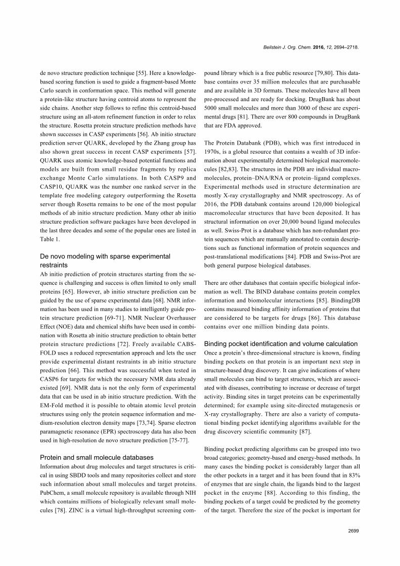
sites of the protein [91]. The SiteHound program is another

energy-based method that uses two kinds of probes; a carbon

probe and a phosphate probe which are used to identify the

binding sites for drug-like molecules and phosphorylated

ligands (such as ATP) respectively [92]. The best ligand

binding site identified in HIV-1 protease by SiteHound is

shown in Figure 4. This ligand binding site is the known inhibi-

tor binding site in HIV-1 protease. Another energy-based

method, FTMAP, uses 16 probes in identifying hot spots in

structures and was more recently extended to include any user

provided small molecule as an additional probe [93,94]. Many

other binding pocket finding programs exist. PEP-SiteFinder

[95], SiteMap available through Schrodinger [96] and MolSite

[97] are a few of these programs.

Figure 4: The best ligand binding site identified by SiteHound in HIV-1protease. The ligand binding pocket is shown in blue spheres and isthe known inhibitor binding site of HIV-1 protease.

When the binding pocket of a target is known one significant

characteristic to be calculated is its binding pocket volume.

With this information elimination of ligands that are too bulky

to fit in the pocket can be done during the lead identification

process. One algorithm that calculates the volume of a binding

pocket is POVME (POcket Volume MEasurer) [98]. McVol is

another standalone program that can identify and calculate the

volume binding cavities in protein structures by using a Monte

Carlo algorithm [99].

Scoring functions used in dockingIn molecular docking, how well a drug binds to its target is de-

termined by the binding affinity prediction of the pose. This is

done by scoring. Scoring is used to evaluate and rank the

target–ligand complexes predicted by docking algorithms.

Scoring functions are used in SBDD for scoring and evaluating

protein–ligand interactions [100,101]. The scoring function

used by docking algorithms is a crucial part of the algorithm. It

is used in the exploration of the binding space of the ligand and

also in the evaluation of target–ligand complexes in molecular

docking. The scoring functions can be categorized into know-

ledge-based [102,103], force-field based [104,105], empirical

[106,107] and consensus [108,109]. These will be discussed

below. The accuracy of different scoring functions has been

evaluated in the literature [110-113]. These comparative studies

that evaluate docking method scoring functions use evaluation

criteria such as binding pose, binding affinity and ranking of

true binders [114]. Wang et al. evaluated the performance of

fourteen different scoring functions using 800 protein–ligand

complexes in the PDBbind database [113]. The performance

was evaluated by the predicted binding affinities of

protein–ligand complexes by different scoring functions. Ac-

cording to this study X-Score, DrugScore and ChemScore were

among the best performing scoring functions. Ferrara et al. used

nine scoring functions and assessed the performance of these

functions using 189 protein–ligand complexes [110]. They

found that ChemScore shows the best correlation for experi-

mental binding energies and predicted binding scores. In

another study done by Marsden et al., calculated binding free

energies with knowledge-based potential function Bleep agreed

best with experimental binding constants [115].

Knowledge-based scoring functionsKnowledge-based scoring functions are statistical potentials and

are derived from experimentally determined protein–ligand

information. The frequency of occurrence of interactions of a

large number of target–ligand complexes are used to generate

these potentials. The basis of these potentials is the Boltzmann

distribution. The frequency of occurrence of atom pairs is con-

verted into a potential using Boltzmann’s distribution of states.

Since these potentials use target–ligand complex data already

available, they are highly dependent on the dataset used to

create them. DrugScore uses knowledge-based potential func-

tions to predict binding affinity [116]. Other knowledge-based

scoring functions include the PMF (Potential of Mean Force)

[117] and Bleep [118].

Force-field-based scoring functionsForce-field based energy functions are developed using clas-

sical molecular mechanics. Electrostatic (coulombic) interac-

tions and van der Waals interactions (Lennard-Jones potential)


2701

contribute to the interaction energy between a target–ligand

complex. Two of the most widely used molecular mechanical

force-fields are CHARMM [119] (Chemistry at HARvard

Macromolecular Mechanics) and AMBER [120] (Assisted

Model Building and Energy Refinement) which have been built

mainly for molecular dynamics simulations. The molecular

docking program DOCK [121] uses force-field based scoring

functions derived from molecular dynamics force-field

AMBER.

Empirical scoring functionsEmpirical scoring functions are obtained by using data from ex-

perimentally determined structures and fitting this information

to parameters. The idea here is that the binding free energy is

calculated as the weighted sum of terms that are uncorrelated.

These terms can be the number of hydrogen bonds, hydro-

phobic effect, and different types of contacts and their types etc.

Regression analysis is usually done to obtain weights of the

terms using experimental target–ligand complexes with known

binding free energy data [122]. Unlike knowledge-based

scoring functions, which are obtained by directly converting

frequency of occurrence of different interactions into potentials

using Boltzmann principle, these functions take into account

multiple terms or contributions and find the best weights for

each term using regression analyses. The HYDE scoring func-

tion is an empirical energy function which is a part of

BioSolveIT tools [123]. Here the binding energy of a

target–ligand complex is solely estimated by a hydrogen bond

term and a dehydration energy term. ChemScore [122] and

SCORE [124] are two other scoring functions that are also

empirical.

Consensus-based scoring functionsCurrent scoring functions are not perfect and no one scoring

function can do well in every docking complex studied.

Consensus scoring was introduced to combine different scoring

functions in the hope that it can balance out errors and improve

accuracy [125]. Consensus scoring function X-CSCORE [126]

was developed by combining three different empirical scoring

functions, namely Bohm’s scoring function [127], SCORE and

ChemScore. Another example of consensus scoring is Multi-

Score [128]. This score function is a combination of eight

different scoring functions and have shown improved

protein–ligand binding affinities.

Protein–ligand docking algorithmsIn docking, predictions are made on how intermolecular com-

plexes are formed between a target and a ligand. These algo-

rithms search for the best target–ligand poses with the right con-

formational state and relative orientation. The algorithms also

crudely estimate the binding affinities of the target–ligand com-

plexes in terms of scoring. The docking algorithms therefore

comprise a search algorithm that searches the conformational

space to find docking poses and a scoring function to predict the

affinity of the ligand in that pose. Computationally docking a

target structure to a molecule is a challenging process. Even

when target flexibility is ignored there are still a huge number

of ways a molecule can be docked. The total number of possible

modes increases exponentially as the size of the two docked

molecules increases. Therefore efficient search methods that are

fast and effective, and reliable scoring functions are critical

components of docking algorithms.

Once a target protein structure is known and a potential drug

binding site has been identified, small molecules that bind to

this site need to be determined. In drug discovery, docking algo-

rithms are used to find the best fit between a target and a small

molecule drug. Docking algorithms require a target protein

structure and a library of small molecules. The target protein

structure is usually determined using experimental methods

such as X-ray crystallography and NMR, or else it is computa-

tionally modeled. Molecular docking aims to predict the

binding mode and binding affinity of a protein–ligand complex.

A library of small molecules is virtually placed (docked) into

the desired protein–target binding site and thousands of possible

poses of binding are obtained and evaluated. The pose which is

scored with the lowest energy is predicted to be the best

possible binding mode. The models are evaluated using a

scoring function and the poses are ranked and a group of high

ranking compounds are chosen for the next step of experimen-

tal verification.

One of the very first studies that developed algorithms to eval-

uate docking poses by looking at steric overlaps was published

in the 1980s [129]. Ever since then many docking algorithms

have been developed [130-135]. Popular molecular docking

programs include Glide [131], Fred [136], AutoDock3 [137],

AutoDock Vina [134], GOLD [138] and FlexX [139].

AutoDock3 uses an empirical scoring function that has five

terms. These terms are weighted with experimental

target–ligand data. It can model side chain flexibility of the

target molecule. AutoDock Vina is the new generation of

AutoDock. The scoring function used in AutoDock Vina is a

hybrid scoring function that combines knowledge-based and

empirical scoring functions [134]. GOLD uses a force-field

based scoring function and allows the ligand to be fully flexible.

It allows target side chain flexibility to be taken into account.

FlexX is an incremental fragment-based docking algorithm

where the conformational space sampling is done using a tree-

search method. It is an ensemble method that can incorporate

target structure flexibility. The scoring function is a modified

version of empirical Bohm’s scoring. Glide is a highly popular


2702

docking algorithm that uses an empirical scoring function [131].

Fred, by OpenEye Scientific, finds protein–ligand docking

poses by using a non-stochastic exhaustive method. It uses

filters that take shape complementarity into account and the top

scoring poses selected are further optimized [136]. Docking

algorithms are discussed in detail in reviews [140-142] and

comparative assessment of algorithms have been done

[112,143-145]. Zhou et al. evaluated the performance of several

flexible docking algorithms by calculating enrichment factors

for a set of pharmaceutical target–drug complexes and found

that Glide XP was superior to other methods tested [144]. The

study done by Perola et al. shows that Glide is superior to other

methods tested for the prediction of binding poses but virtual

screening is mostly target-dependent [112].

The best docking algorithm should be the one with the best

scoring function and the best searching algorithm. The perfor-

mance of various docking algorithms has been evaluated and

they are able to generate docked ligand conformations that are

similar to experimental complexes [146]. Compared to co-crys-

tallized X-ray structures of target–ligand complexes docking

results can sometimes even predict poses with RMSDs of less

than 1 Å [147]. Measuring RMSD (root mean square deviation)

is the most common way to compare the structural

similarity between two superimposed structures. RMSD is

given by:

where n is the number of atom pairs and dx is the distance be-

tween the two atoms in the xth atom pair.

However, it is important to note that no single docking method

performs well for all targets and the quality of docking results is

highly dependent on the ligand and the binding site of interest

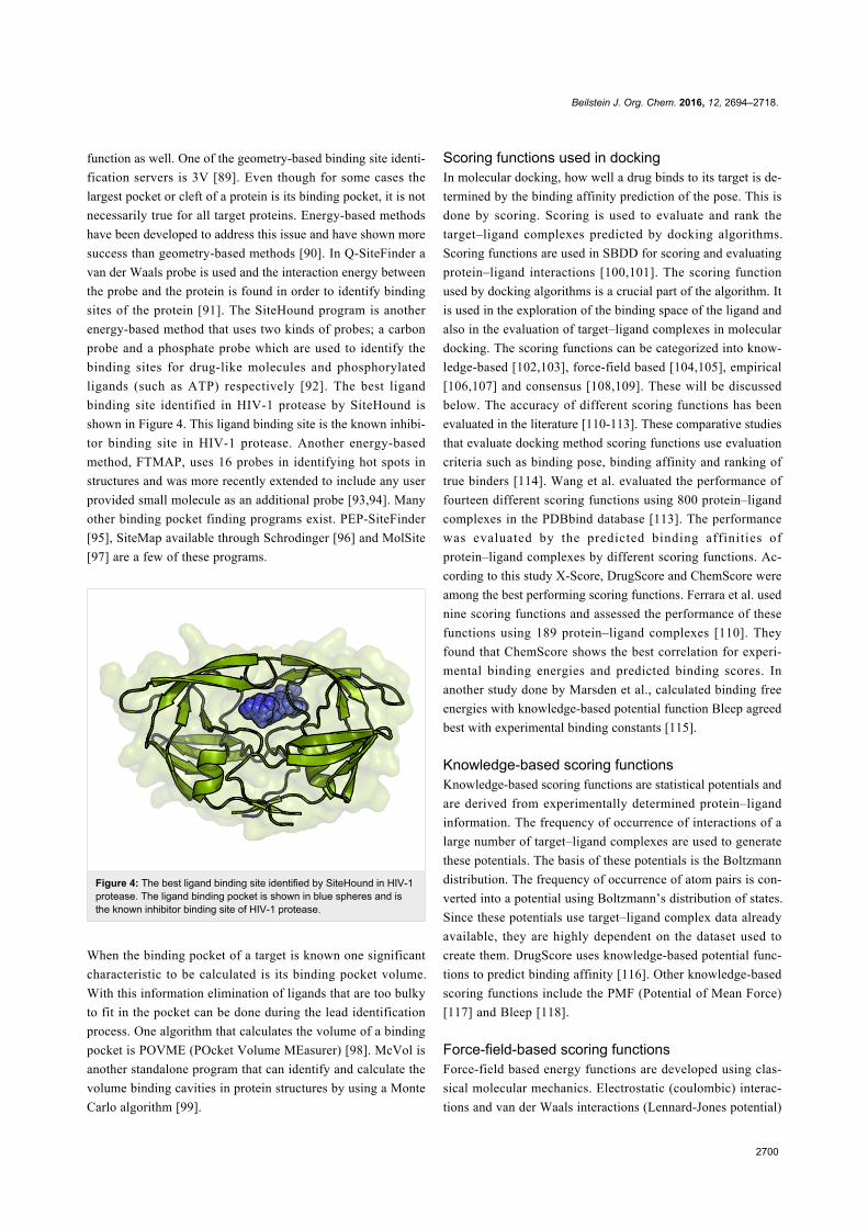
[148-150]. The best four binding poses predicted for the known

inhibitor Dorzolamide binding to carbonic anhydrase II ob-

tained by AutoDock Vina are shown in Figure 5.

Preprocessing of target and ligandsTarget and ligand preparation steps are crucial and are often

done before docking is performed to ensure good screening

results [151]. In experimental methods such as X-ray crystallog-

raphy the hydrogen atoms of structures are not generally

present. However, the presence of these atoms and the loca-

tions of these bonds are important for molecule docking algo-

rithms. Additionally, the target protein structures, if used with-

out preprocessing, can give rise to potential issues due to

missing residues, atom clashes, crystallographic waters and

Figure 5: Binding mode prediction. The known inhibitor Dorzolamide isdocked into Carbonic anhydrase II crystal structure (4M2U) (blue)using AutoDock Vina. Four binding poses predicted are shown ingreen, cyan, red and yellow. The molecular structure of Dorzolamide isshown in Figure 3b.

alternate locations. In target preprocessing, missing atoms such

as hydrogen are added and atomic clashes are removed. The

same is true for the ligands that are used. During ligand prepro-

cessing, ligand three-dimensional geometries are predicted. All

possible ionization, stereoisomeric and tautomer states are

assigned [152]. The protonation states of structures are also im-

portant in prediction of docking poses because protonation

states affect how ligands bind to the binding site [100]. Opti-

mizing protonation states of binding pockets and also positions

of polar hydrogens can lead to identifying the most native-like

docking poses.

SPORES is one program that is used for the prepossessing of

proteins for protein–ligand docking. It can generate different

protonated states, tautomeric states and stereoisomers for pro-

tein structures [152]. LigPrep from the Schrodinger Suite [153]

allows to obtain all-atom 3D structures of ligands. It is avail-

able through the maestro interface or by command line. A web-

based ligand topology generating server, PRODRG, can

generate 3D coordinates for ligands that are of equal or better

quality than other methods [154].

De novo ligand designBy using fragment-based de novo ligand design it is possible to

assemble molecules that are drug-like with much less search

space having to be explored. In some cases, de novo drug

design is less successful in generating drug candidates com-

pared to other methods such as high-throughput virtual

screening methods for large databases. One limitation of this

approach can be attributed to its high complexity. When a high-

resolution target structure is available, ligand growing programs


2703

such as biochemical and organic model builder (BOMB) can be

used to design ligands that bind to the target without using

ligand databases [155,156]. Using BOMB it is possible to grow

molecules by adding substituents into a core structure. It has

been possible to design inhibitors for Escherichia coli RNS

polymerase using the de novo drug design program SPROUTS

[157]. In another study that used the SPROUT program, novel

inhibitors were developed for Enterococcus faecium ligase

VanA using hydroxyethylamine as the base template structure

[158]. It is generally necessary to synthesize molecules that are

obtained by de novo drug design. Whereas when using virtual

screening methods, since the screening is usually done with

databases of commercially available molecules, it is possible to

purchase these molecules without the need to synthesize them.

LigMerge is another novel algorithm that can generate novel

ligands for drug targets [159]. It uses known ligands of a target

and generates models with similar chemical features by finding

the maximum common substructure of known ligands. Chemi-

cal groups of superimposed ligands are attached to the common

substructure. This produces different molecules that have fea-

tures of the known ligands. The algorithm is able to identify

novel ligands for several known drug targets that have pre-

dicted affinities higher than their known binders. The Auto-

Grow software is a drug molecule optimizing program. It can be

used to optimize ligands according to various properties and

binding affinities and is available to download [160]. If two

fragments bind to two non-overlapping nearby sites on a target

protein, these fragments can be joined to obtain a possible new

drug molecule. In the SILCS (site identification by ligand

competitive saturation) method, molecular dynamics simula-

tions are used to identify fragments that bind to a target

[161,162]. SILCS uses explicit molecular dynamics simula-

tions where the target molecule is simulated in an aqueous solu-

tion that contains different fragments. Using multiple simula-

tions SILCS determines high probability binding areas of the

target for the different fragments which can be used in frag-

ment-based drug design. Another de novo ligand design

program is LigBuilder which is available for download

[163,164]. Here the ligands are either grown or linked by user’s

choice, and an empirical scoring function is used to estimate

binding affinities.

Structure-based virtual high-throughput screening(VHTS)Structure-based virtual high-throughput screening (VHTS) is

large scale in silico screening of drug molecules in databases of

small molecule compounds for a target of interest. Here a target

is “screened” against a library of drug-like molecules and

binding affinities of the ligands to the target are estimated using

the scoring functions described previously. In addition to

finding the best docking pose VHTS also ranks docking results

according to their predicted affinities for the entire database.

Since large databases are screened, it is important that the

target–ligand docking algorithms used in VHTS are both fast

and sufficiently accurate, to be able to identify a subset of

possible drug compounds. Small molecules that are predicted to

bind to the target with high affinity can be identified. These

“hits” are then generally further optimized and subsequently

tested experimentally. With improving computational resources

and parallel processing cluster availability, it is now possible to

screen millions of compounds within a matter of hours or days.

Because of VHTS it is possible to experimentally test a rather

small number of molecules. Testing thousands of available

compounds in databases experimentally may no longer be

necessary.

Structure-based high-throughput screening has been used to

identify inhibitors of protein kinase CK2 targeting its ATP

binding site [165]. CK2 is an important target in developing

antitumor drugs. About 400,000 compounds have been

screened, from which 12 hits were selected for evaluations

using in vitro assays. Out of these hits a novel drug was identi-

fied which was able to inhibit CK2 enzymatic activity with an

IC50 of 80 nM. At the time it was discovered, this drug was

considered one of the most potent drugs for a protein kinase. In

another study, VHTS was used to show proliferator-activated

target agonistic behavior with Sulfonylureas and Glinides

binding [166]. This finding has implications in the treatment of

type-2 diabetes and it was also confirmed by experimental

assays. Recently, virtual screening has been used to find

anitiviral inhibitors that target the Ebola virus. This study found

a lead candidate from the TCM database that shows a decrease

in activity for the protein encoded by the virus [3]. This promis-

ing candidate also shows good pharmacokinetic properties.

VHTS was also used to find a novel quinolinol that binds to

MDM2 in a fashion mimicking the binding of p53 and inhibit

the MDM2-p53 interaction [167]. This inhibition can activate

p53 in cancer cells. There are many more examples where

VHTS has been used in drug discovery studies [168-172].

Target flexibility in molecular dockingExperimental methods such as X-ray crystallography represent

proteins as static structures. However proteins are dynamic

systems and show internal motions. The functionality of pro-

teins is governed by their internal dynamics. In order to explain

their function it is important to understand their dynamic char-

acteristics [173]. In the first molecular docking attempts in the

1980s, the rigidity of the target protein was always assumed

[129]. This has not changed significantly until recently; some

newer docking algorithms can account for target flexibility. It is

important to account for target protein flexibility because pro-

tein structures are dynamic in nature and their structures change


2704

upon binding of drug molecules. These changes may involve

overall backbone structure rearrangements or they can be subtle

where only the side chains near the ligand binding site change

to accommodate the bound ligand. However, this dynamic

nature of targets is frequently ignored and protein flexibility is

underrepresented in CADD. In conventional docking algo-

rithms the target is held rigid while the ligand molecule is gen-

erally assumed to be flexible. This rigid body docking of

ligands to the target is not realistic and can give misleading

results because targets are actually able to freely undergo side

chain and backbone movements as a result of ligand binding by

an induced fit mechanism [174]. Two approaches that can be

taken to account target flexibility are induced fit docking

methods and ensemble-based screening methods.

In induced fit docking the target protein structures are modeled

as flexible, not rigid. They are able to accommodate induced fit

that is caused by the ligand molecule binding to it. Schrodinger

has introduced induced fit docking protocols through Glide

[174]. RosettaLigand also accounts for target flexibility and

shows success in predicting target–ligand poses. All residue

side chain flexibility of the ligand binding pocket and target

backbone flexibility are taken into account by RosettaLigand.

This method uses a Monte-Carlo-based minimization algorithm

and the Rosetta full-atom energy function [175].

Ensemble-based docking is an alternative method to induced fit

docking. With ensemble-based screening methods there is no

need to choose flexible residues of interest to binding [176-

180]. The relaxed complex scheme (RCS) method uses struc-

ture dynamics and docking algorithms in combination to

account for target flexibility [181,182]. One successful applica-

tion of RCS was reported for HIV integrase. MD simulations

that were performed with the holo-structure of HIV integrase

bound to a known ligand showed signs of a novel binding

pocket opening in close proximity to its active site [183]. RCS

ligand docking showed that this binding site is a possible

binding pocket for drug molecules. This finding paved the way

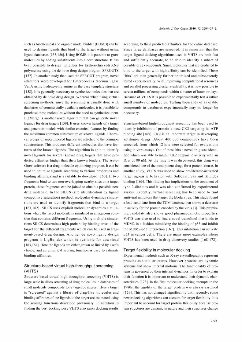
for the development of raltegravir to treat HIV infection which

was later approved by the FDA (Figure 6) [184,185]. These en-

semble-based screens use an experimentally determined starting

target structure and use various methods to generate target

structure ensembles. These methods include molecular dynam-

ics simulations [186], Monte Carlo simulations [187], enhanced

sampling [177] or just simply experimental ensembles from

NMR or multiple crystal structures, to generate an ensemble of

conformations based on the starting target structure. By doing

so, conformations of the target structure that are relevant to the

biological function which are not accessible by experimental

structure determination, can be obtained. The trajectories can be

clustered to obtain a set of representative conformations. The

difference here is that instead of using one structure, an ensem-

ble of structures is used in docking. Due to the range of confor-

mations generated by these methods a more representative

set of small molecules can now bind to the ensemble

[6,188,189].

Figure 6: The molecular structure of Raltegravir. Raltegravir is an FDAapproved drug used in the treatment of HIV infection.

Enhanced sampling methodsEnsemble-based methods which are typically employed to

account for target flexibility use enhanced sampling methods.

One of the tools that is extensively and routinely used to under-

stand protein motions and conformational space that is acces-

sible for protein structures is molecular dynamics (MD) simula-

tions [190]. The most widely used molecular dynamics soft-

ware packages are NAMD [191], GROMACS [192] and

AMBER [120]. The typical time-scale of a molecular dynamics

simulation is in the order of nanoseconds to microseconds.

However to capture biologically important conformational tran-

sitions, frequently it is important to probe dynamics in the order

of milliseconds. Simulating on that timescale makes it possible

to overcome high-energy barriers in some important biological

transitions. With conventional all-atom MD simulations and

typically available computational resources this can be a very

time consuming process. Millisecond-scale MD simulations are

possible with high speed supercomputers, although most

computational scientists do not have access to such powerful

machines [193]. This is considered a major limitation of MD. It

may take months to complete a one microsecond molecular dy-

namics run on a system having around 25000 atoms on

24 processors [194]. Enhanced sampling methods have been

introduced to address this issue [176,195]. With enhanced

sampling methods it is possible to find conformational states

that are relevant to the function of proteins that are not explored

in conventional MD. Enhanced sampling methods introduce a

bias on the system being simulated. Several methods of en-

hanced sampling are introduced in literature, including: acceler-

ated molecular dynamics [196,197], metadynamics [198,199],

umbrella sampling [200] and temperature-accelerated molecu-

lar dynamics [201,202].


2705

Accelerated molecular dynamics (aMD) simulations reduce the

energy barrier of wells or in other words raise the energies of

the wells that are below a certain threshold energy [203]. This

leaves the high-energy states above the cutoff unaffected. When

the original energy of the system is below the calculated energy,

an additional potential term is added (a boost potential), thereby

allowing energy barriers to be smaller. This makes it possible

for the system to access conformations which are not accessible

without the energy barrier reduction [203-205].

In metadynamics a history-dependent bias potential (which is a

function of a set of collective variables) or a force is added to

the Hamiltonian of the system to accelerate the system in

consideration by pushing it from the local energy minimum

[199]. It is important that the collective variables used can

describe the initial, final and intermediates states. Commonly

used collective variables are interatomic angles, dihedrals and

distances. By doing so, it is possible to sample rare events that

are otherwise not sampled by conventional MD. Finding the set

of collective variables however is challenging especially when

the simulated biological system is more complex. Recently, in-

duced fit docking has been coupled with metadynamics to

predict protein–ligand complexes in a reliable way. By incorpo-

rating metadynamics with induced fit methods, the predictive

power of these methods can be enhanced without requiring too

much computational resources [4].

The umbrella sampling technique is used to calculate free

energy differences in systems [200]. An additional energy term

or a bias potential is introduced to the system along a reaction

coordinate. This bias potential can then drive the system from

the reactant state to the product state. Each of the intermediate

states is simulated by MD. Most of the time, for reasons of

simplicity, bias potentials are applied as harmonic potentials

[200,206].

In temperature-accelerated MD, the system simulation is done

at a high enough temperature which makes it possible to accel-

erate the sampling. Temperature accelerated MD has been used

in the study of ligand dissociation from the inducer binding

pocket in the Lac repressor protein [202]. By using this method,

it was possible to sample the dissociation trajectories in a rela-

tively short period of time to capture the ligand dissociation.

The replica exchange method runs a number of independent

replicas in different ensembles of the systems at different tem-

peratures and allows exchange of replica coordinates to take

place between these ensembles [207]. This method can also en-

hance sampling in cases where the energy landscape of a

system has many minima and where it is not possible to

cross the barriers between them during standard simulation

times.

Rigorous binding free energy calculationsRigorous binding free energy calculations can be used to more

precisely estimate the binding affinity of target–ligand com-

plexes and these affinities can be used to rank the fit of drug

molecules for a particular target. Binding affinities can be used

to infer how drug binding will be affected by target mutations

[208]. The potency of a drug is assumed to be directly related to

the target–drug molecule binding affinity. Therefore it is impor-

tant to be able to accurately predict the target–ligand binding

affinity [209]. Currently the most accurate approaches to calcu-

late binding free energies are rigorous approaches [210]. Monte

Carlo algorithms and molecular dynamics simulations are used

for generating ensemble averages to model complexes in the

presence of explicit water molecules using classical force-fields.

Two rigorous binding free energy approaches are the free

energy perturbation (FEP) methods and thermodynamic integra-

tion (TI) methods [211-215]. These methods are much more

accurate than virtual screening. Both of these methods are

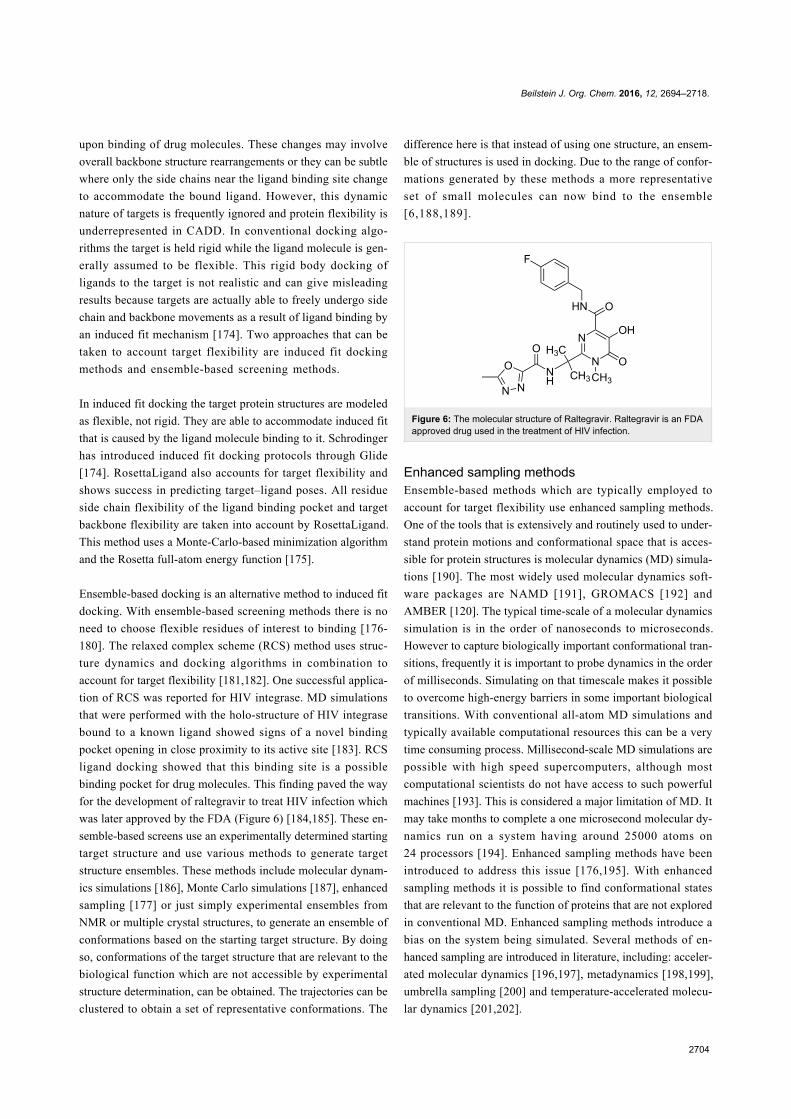
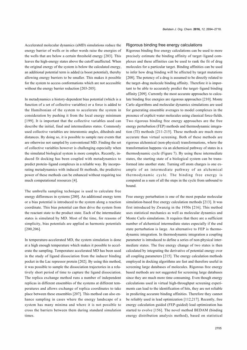
rigorous alchemical (non-physical) transformations, where the

transformation happens via an alchemical pathway of states in a

thermodynamic cycle (Figure 7). By using these intermediate

states, the starting state of a biological system can be trans-

formed into another state. Turning off atom charges is one ex-

ample of an intermediate pathway of an alchemical

thermodynamic cycle . The binding free energy is

computed as a sum of all the steps in the cycle from unbound to

bound.

Free energy perturbation is one of the most popular molecular

simulation-based free energy calculation methods [213]. It was

first introduced by Zwanzig in the 1950s [216]. This method

uses statistical mechanics as well as molecular dynamics and

Monte Carlo simulations. It requires that there are a sufficient

number of alchemical intermediate states especially if the end

state perturbation is large. An alternative to FEP is thermo-

dynamic integration. In thermodynamic integration a coupling

parameter is introduced to define a series of non-physical inter-

mediate states. The free energy change of two states is then

calculated by integrating the derivative of potential energy over

all coupling parameters [215]. The energy calculation methods

employed in docking algorithms are fast and therefore useful in

screening large databases of molecules. Rigorous free energy

based methods are not suggested for screening large databases

since they are much more time consuming. Even though energy

calculations used in virtual high-throughput screening experi-

ments can lead to the identification of hits, they are not reliable

in predicting accurate binding affinities. Therefore they cannot

be reliably used in lead optimization [112,217]. Recently, free

energy calculation guided (FEP-guided) lead optimization has

started to evolve [156]. The novel method BEDAM (binding

energy distribution analysis method), based on statistical


2706

Figure 7: An example alchemical thermodynamic cycle for a protein–ligand binding free energy calculation. The protein is shown in blue spheres. Theligand, depicted in solid black, indicates there are no coulombic or van der Waals (VDW) interactions with the environment. The ligand, depicted insolid orange, indicates there are coulombic and VDW interactions with its environment. The systems that are subjected to simulations in each cycleare highlighted in blue boxes. All simulations are run in a water environment. The first step is to add restraints between ligand and the protein in orderto keep the ligand confined to the binding pocket and to avoid the ligand leaving the pocket when its interactions are removed. The systems withrestraints turned on are indicated by red hexagons. In the next step the coulombic and VDW interactions of the ligand are removed. This step is fol-lowed by the removal of the restraints applied to the ligand. Next the coulombic and VDW interactions of the ligand are turned on such that the ligandis in contact with solvent. Summing up the free energy changes along the thermodynamic cycle would give the protein–ligand binding free energy.

mechanics, is used to calculate binding free energies of target-

ligand complexes [218]. BEDAM is an implicit solvent method

that is implemented using Hamiltonian replica exchange molec-

ular dynamics. Recently BEDAM showed success in the

SAMPL4 (statistical assessment of the modeling of proteins and

ligands) challenge in predicting free energies of binding for a

set of octa-acid host–guest complexes [219]. VM2 is another

method used in target–ligand binding energy calculations which

falls between rigorous free energy calculation methods and ap-

proximate docking and scoring algorithms in its complexity

[220]. It is an implicit solvent method and uses empirical force-

fields. Its implementation is based on mining minima end point

method (M2). In this method the binding site is taken to be fully

flexible and the other parts of the target are kept fixed. Due to

the flexibility of the binding site, it can adapt according to dif-

ferent bound ligands. The free energy is estimated to be the sum

of all local energy minima.

Lead optimization and assessment of ADME anddrug safetyWhen hits are obtained for a target structure by screening small

molecule databases, the next step usually is lead optimization.

During lead optimization, the effectiveness of promising hits

obtained is generally enhanced while at the same time obtain-

ing the desired pharmacological profiles to reach the required

affinity, pharmacokinetic properties, drug safety, and ADME

(absorption, distribution, metabolism, and excretion/elimina-

tion) properties. By increasing the affinity of a drug to the target

its potency (efficacy) can be increased. The free energy of

binding of a drug is a measurement of the potency of a drug to

the target of interest. This could be done by doing alchemical

free energy calculations in complex with running molecular dy-

namics simulations. One simulation starts with the target–ligand

bound complex and slowly removes the ligand, and the other

slowly removes the ligand from the solution. It is possible to


2707

find chemical changes of a possible drug candidate that can

improve its potency using alchemical free energy calculations.

This is done by gradually converting one atom of the

ligand to another and calculating the binding affinity.

These a f f in i ty changes wi th a tom modi f i ca t ions

can be used as guides for improving potency of drug candidates

[194].

The permeability of a drug through the intestines and solubility

are both important factors that affect drug absorption [221].

Therefore, in silico prediction of solubility and membrane

permeability of drugs is an important part of lead optimization

[222]. If an orally administrated drug has poor solubility or a

high dissolution rate, the drug tends to be excreted by the body

without entering the blood stream. This causes the drug to be in-

efficient and can even cause other biological side effects. To ex-

perimentally measure the solubility, the synthesis of the drug is

needed which is a time consuming process. However, predicting

solubility using computational methods is fast. It is possible to

perform solubility calculations on large molecule libraries with-

out needing a lot of computational resources. The solubility data

can assist medicinal chemists to evaluate the drug candidates

without having to synthesize molecules at all. This greatly

reduces the costs of molecule synthesis and time for experimen-

tal solubility measurements. Huynh et al. used an in silico

method for the prediction of solubility of docetaxel (DTX), an

anti-cancer molecule used to treat various types of cancer [223].

In this study solubility parameters for DTX were obtained using

MD simulations. This in silico model was in agreement with the

experimental solubility of DTX. Simulation-based approaches

are frequently used in computational permeability prediction

[224,225]. In one study, trajectories obtained by molecular

dynamic simulations have been used to obtain diffusion coeffi-

cients of permeation of drug-like molecules through the blood-

brain barrier [225]. In silico approaches to predict drug solu-

bility in both aqueous media and DMSO are discussed in a

review [226].

Human intestinal absorption of a candidate drug is of high

importance because it can affect the bioavailability of a drug.

According to the Lipinski’s ‘Rule of 5’, poor absorption or

permeation is more likely when: there are more than 10 H-bond

acceptors, more than 5 H-bond donors, Log P is over 5, and the

molecular weight is over 500 [227]. There are extensions of the

Rule of 5 in predicting drug-likeliness as well [228]. One such

extension later proposed is the ‘Rule of 3’ which was used in

the construction of fragment libraries for lead generation [229].

These rules are generalized rules for evaluating the drug-like-

ness and bioavailability of compounds. Various statistical and

mathematical models have been based on these rules and their

extensions. Machine learning algorithms such as neural

networks have been used in the prediction of drug-likeness and

bioavailability [230,231].

QikProp is an ADME program offered by Schrodinger that

predicts pharmaceutically relevant and physically significant

descriptors for small drug-like molecules [232]. The VolSurf

package can be used to calculate ADME properties and

generate ADME models [233]. These ADME models can then

be used to predict the behavior of novel molecules. It can also

be used to find molecules with similar ADME properties as

active ligands of interest. FAF-Drugs2 is an ADME and toxici-

ty filtering tool that can calculate physicochemical properties,

toxic and unstable groups, and key functional components

[234]. Even though many possible drug molecules go to experi-

mental verification stage or even animal models, they do not

reach clinical trials. This is mostly due to the fact the drugs

have poor pharmacokinetic properties and toxicity [235]. Thus

filters for ADME properties are important for drug screening

[236]. Computational ADME methods have advanced greatly in

the last few decades and pharmaceutical companies are showing

great interest in this area [237].

Ligand-based drug design (LBDD)The main alternative to SBDD is LBDD. In the case where the

potential drug target structure is unknown and predicting this

structure using methods such as homology modeling or ab initio

structure prediction is challenging or undesirable, the alterna-

tive protocol to use is Ligand-based drug design [238,239]. Im-

portantly, however, this method relies on the knowledge of

small molecules that bind to the target of interest. Pharma-

cophore modeling, molecular similarity approaches and QSAR

(quantitative structure–activity relationship) modeling are some

popular LBDD approaches [240]. In molecular similarity

methods, the molecular fingerprint of known ligands that bind

to a target is used to find molecules with similar fingerprints

through screening molecular libraries [241]. In ligand-based

pharmacophore modeling, common structural features of

ligands that bind to a target are used to do the screening [242].

QSAR is a computational method that models the relationship

between structural features of ligands that bind to a target and

the corresponding biological activity effect [243].

Similarity searchesThe main idea of similarity-based or fingerprint-based ap-

proaches is to select novel compounds based on chemical and

physical similarity to known drugs for the target. Ligand simi-

larity search methods are simple but effective approaches based

on the theory that structurally similar molecules tend to have

similar binding properties [244]. These similarity measures do

not take into account information about activities of known

binders of the target. G-protein-coupled target GPR30 specific


2708

agonist that activates GPR30 was developed using similarity

searches. The final similarity score that was used comprised a

2D score and a 3D structure similarity component [245-247].

Pharmacophore modelingA pharmacophore is a molecular framework that defines the

essential features responsible for the biological activity of a

compound. When structural information about the drug target is

limited or not known, pharmacophore models may be built

using the structural characteristics of active ligands that bind to

the target [248]. When 3D information of the target structure is

known this binding site information can also be used in gener-

ating pharmacophore models [242]. Pharmacophore models that

use chemical features such as acidic/basic residues and hydro-

gen bond acceptors and donors are found to be the most effec-

tive models [248]. Pharmacophore modeling has also been used

in virtual screening of drugs in large databases [249]. There are

programs developed to identify and generate pharmacophore

models such as DISCO, GASP and Catalyst. It has been re-

ported that GASP and Catalyst perform better than DISCO in

reproducing the pharmacophore models [250]. One naturally

occurring anti-cancer molecule identified using QSAR is I3C

(indole-3-carbinol). However, this molecule has never gone past

clinical trials due to its low potency. This active compound was

optimized using ligand-based pharmacophore modeling to

develop highly potent analog SR13668 which is a novel drug

that shows to be highly potent against several cancer types [5].

Pharmacophore model construction steps can be summarized as

follows:

1. The active compounds known to be binding to the

desired target, that are also known to have the same

interaction mechanism, are identified either by a litera-

ture search or a database search.

2. (a) For a 2D pharmacophore model essential atom types

and their connectivity are defined (b) For a 3D pharma-

cophore model the conformations are defined using

IUPAC nomenclature.

3. Ligand alignment or superimposition is used to find

common features required in binders.

4. Pharmacophore model building.

5. Ranking of the pharmacophore models and selecting the

best models.

6. Validation of pharmacophore models.

QSAR (quantitative structure–activity relationships)QSAR methods are based on statistics that correlate activities of

target drug interactions with various molecular descriptors. The

basis of the QSAR method is the fact that structurally similar

molecules tend to show similar biological activity [251]. These

models describe mathematically how the activity response of a

target, that binds a ligand, varies with the structural features of

the ligand. QSAR is obtained by calculating the correlation be-

tween experimentally determined biological activity and various

properties of small ligand binders [243]. QSAR relationships

can be used to predict the activity of new drug molecule

analogs.

In order to quantify the activity of a drug molecule, several

values can be used. Half maximal inhibitory concentration

(IC50) and inhibition constant (Ki) are the most commonly used

measures. QSAR models, unlike the pharmacophore models,

can be used to find the positive or negative effect of a particu-

lar feature of a drug molecule to its activity. QSAR methods

have been used successfully on various drug targets such as

carbonic anhydrase [252,253], thrombin [254,255] and renin

[256]. Different machine learning techniques have also been

used in constructing QSAR models [257-259]. In classical or

2D QSAR methods, the biological activity is correlated to

physical and chemical properties such as electronic hydro-

phobic and steric features of compounds [260]. In more ad-

vanced 3D QSAR methods, in addition to physical and

geometric features of active drug molecules, quantum chemical

features are also used. Recently QSAR models have also been

developed for membrane systems [261].

The basic steps (Figure 8) of the QSAR method can be summa-

rized as follows:

1. The active molecules that bind to the desired drug target

and their activities are identified through a database

search, a literature search, or HTS experiments.

2. Identification of structural or physicochemical molecu-

lar features (fingerprint) affecting biological activity (e.g.

bond, atom, functional group counts, surface area etc.).

3. Building of a QSAR between the biological activity and

the identified features of the drug molecules.

4. Validation of the QSAR biological activity predictive

power.

5. Use of the QSAR model to optimize the known active

compounds to maximize the biological activity.

6. The new optimized drug molecule activities are tested

experimentally.

Success of a QSAR depends on the molecular descriptors

selected and the ability of these models to predict biological ac-

tivity. If there is not enough activity data to extract patterns,

QSARs cannot perform well. Therefore, this method requires a

certain minimum amount of training data in order to build a

good predictive model and it is often linked to high-throughput

screening. Statistical methods have been used in linear QSAR to

pick molecular descriptors that are important in predicting the


2709

Figure 9: A few drugs discovered with the help of ligand-based drug discovery tools. (a) Zolmitriptan: used as a treatment to migraine (b) Norfloxacin:used in urinary tract infections and (c) Losartan: used to treat hypertension.

Figure 8: Schematic diagram showing the steps involved in QSAR.Known drug molecule activity and descriptor data is obtained and themathematical model of QSAR is built such that descriptors can predictthe activity of each molecule. The predictive power of models are vali-dated and used in predicting activities of novel compounds.

biological activity. MLR (multivariable linear regression) can

be used to find molecular descriptors that have a good correla-

tion with the target–ligand biological activity. It is only possible

to use linear regression methods if the activity descriptor rela-

tion is linear. However the relationship between biological ac-

tivity and the molecular descriptors are not always linear [262].

Machine learning approaches such as neural networks and

support vector machine methods are used to generate QSAR

models to address this issue of non-linear fitting [263-265].

Principal component analysis (PCA) can be used to simplify the

complexity by removing the descriptors that are not indepen-

dent [266]. Once the right set of features is identified and the

QSAR is built, these models can be validated using methods

such as cross validation [267,268]. QSAR models can be used

to predict the biological activity of novel molecules by just

using the molecular features. Thus these models can be used to

screen a database of molecules to find potential active mole-

cules.

Some of the drugs that are on the market with the help of

ligand-based drug discovery are Zolmitriptan, Norfloxacin and

Losartan [8]. Norfloxacin is a drug that is used in urinary tract

infections and was developed using a QSAR model and ap-

proved by the FDA in 1986 [269]. Losartan [270] is used to

treat hypertension and Zolmitriptan [271] is used as a treatment

to migraine (Figure 9).

One difference between pharmacophore models and QSAR is

that the pharmacophore model is constructed based on the

necessary or essential features of an active ligand, whereas

QSAR takes into account not only the essential features but also

the features that affect the activity. One important structural fea-

ture used in both the pharmacophore model and in QSAR is the

volume of the binding site. It is well established that the binding

pocket volume has a big influence on the biological activity. In

the cases where the binding pocket volume is known, elimina-

tion of molecules that are too large to fit in the binding pocket

can be done in early stages of drug discovery process

(see section “Binding pocket identification and volume calcula-

tion”).

Role of machine learning in LBDDMachine learning algorithms can be trained to identify patterns

in data and used to do predictions on test data sets. These algo-

rithms are extensively applied in the field of biology and drug

discovery [272-275]. Machine learning is used in many stages

in the drug discovery pipeline including in the QSAR analysis

stage [276]. Support vector machine (SVM) based algorithms

are commonly used and have been shown to have high predic-

tive power. SVM are often used for classification of sets of bio-

logical data. For example, they can be used to distinguish be-


2710

tween molecules that have high affinity for a target and those

that have no affinity. Machine learning based scoring functions

can also be used in structure-based drug discovery to predict

target–ligand interactions and binding affinities [277]. Com-

pared to conventional scoring functions, machine learning based

scoring functions have often shown comparable or even im-

proved performance. Moreover these algorithms can be trained

to distinguish active drugs from decoys that do not have known

drug activity [278]. Artificial neural networks (ANNs) have

been used in drug discovery as a powerful predictive tool for

non-linear systems [279]. For example, ANNs were used to

construct the QSAR of a set of known aldose reductase inhibi-

tors and biological activities of new molecules were predicted

based on the QSAR [280]. Docking algorithms were then used

to find novel inhibitors that bind to aldose reductase. ANN-

based prediction models are also used in predicting biotoxicity

of molecules as well [281].

ConclusionIn the past 10 years the identification rate of disease-associated

targets has been higher than the therapeutics identification rate.

With considerable rise in the number of drug targets, computa-

tional methods such as protein structure prediction methods,

virtual high-throughput screening and docking methods have

been used to accelerate the drug discovery process, and are

routinely used in academia and in the pharmaceutical industry.

These methods are well established and are now a valuable inte-

gral part of the drug discovery pipeline and have shown great

promise and success. It is cheaper and faster to computationally

predict and filter large molecular databases and to select the

most promising molecules to be optimized. Only the molecules

predicted to have the desired biological activity will be screened

in vitro. This saves money and time because the risk of commit-

ting resources on possibly unsuccessful compounds that would

otherwise be tested in vitro is reduced.

Structure-based and ligand-based virtual screening methods are

popular with most of the applications being directed towards

enzyme targets [282]. Even though structure-based methods are

more frequently used, ligand-based methods have led to the

discovery of an impressive number of potent drugs. In SBDD

knowing the three-dimensional structure of the target of interest

is required. However, in some cases it is not possible to deter-

mine structures of targets using conventional experimental

methods due to experimental challenges. In the cases where ex-

perimental methods fail, computational methods become useful

and potentially necessary for SBDD [23]. In the absence of an

experimentally determined structure or a computationally

generated model for a target of interest LBDD tools can be

used. These tools require the knowledge of active drugs that

bind to the target. LBDD tools such as 2D and 3D similarity

searches, QSAR and pharmacophore modeling have proven

successful in lead discovery.

Experimental methods usually represent proteins as static struc-

tures. However proteins are highly dynamic in character and

protein dynamics play an important role in their functions.

Computational modeling of the flexible nature of proteins is of

great interest and various ensemble-based methods in structure-

based drug discovery have emerged [178]. Molecular dynamics

simulations are widely used in generating target ensembles that

can be subsequently used in molecular docking [178]. Docking

tools have been developed with different scoring functions and

search algorithms. Comparative studies have been performed to

evaluate these scoring functions and docking algorithms in

docking pose selection and virtual screening [112,144,283].

There is no one superior tool that works for all target–ligand

systems. The qual i ty of docking resul ts is highly

dependent on the ligand and the binding site of interest [148-

150].

VHTS methods are useful to screen large small molecule repos-

itories fast and pick a smaller number of possible drug-like mol-

ecules for testing. By reducing the number of possible mole-

cules that need to be tested experimentally, these methods can

help to greatly cut the cost associated with drug discovery

process. Studies have shown that with VHTS it is possible to

identify molecules that are not observed with conventional

high-throughput screening (HTS) experiments [284]. Thus

VHTS methods are frequently used to complement HTS

methods. The molecules selected by both of these methods are

more likely to be possible drug candidates and should be

considered when selecting hits.

Absorption, distribution, metabolism and elimination/excretion

properties, commonly abbreviated ADME, as well as toxicity

are important for the ultimate success or failure of a possible

drug candidate. Adverse effects in animal models or even clini-

cal trials can be reduced by filtering drug candidates by their

ADME properties in early stages. Another important fact to

consider in drug safety studies is how one drug can affect the

metabolic stability of another drug [285]. Some drug–drug

interactions (DDI) could lead to serious health effects; there-

fore, predicting these effects is important but challenging. The

prescription antihistamine terfenadine and antifungal

drug ketoconazole are two examples of drugs that should not be

co-administered [286]. Terfenadine–ketoconazole drug–drug

interactions results in cardiotoxicity. Computational

methods such as pharmacokinetic modeling and predicting

drug–drug interactions using large DDI interaction databases

are successful and are both cost and time saving as well

[287,288].


2711

Currently hybrid structure-based and ligand-based methods are

also gaining popularity. These combined (ligand-based and

structure-based) drug discovery methods are of interest because

they can amplify the advantages of both methods and improve

the protocols [289-291]. One example is the hybrid docking

protocol HybridDock, which incorporates both structure-based

and ligand-based methods [291]. This hybrid method shows sig-

nificantly improved performance in both binding pose and

binding affinity prediction.

CADD has had a significant impact on the discovery of various

therapeutics that are currently helping treat patients. Despite the

successes, CADD also faces challenges such as accurate identi-

fication and prediction of ligand binding modes and affinities

[8]. One of the challenging areas in drug discovery is the phe-

nomenon of drug polymorphism [292]. Drug polymorphism

occurs when a drug has different forms which are identical

chemically but differ structurally. This can have a great impact

on the success of a drug. Different polymorphic forms of a

drug, which have different solid-state structures, can differ in

solubility, stability and dissolution rates. Drug polymorphism

can affect the bioavailability, efficacy and toxicity of a drug.

One polymorphic form that is responsible for a particular drug

effect may differ if a different polymorphic form of the same

drug is administered. Using techniques such as spectroscopy it

is possible to characterize drugs having different polymorphic

forms.

Protein–protein interactions (PPIs) pose another challenge in

drug discovery. PPIs are involved in many cellular processes

and biological functions that are linked to diseases. Therefore,

small molecule drugs that aim at PPIs are important in drug

discovery [293]. It is of interest to develop therapeutics that can

either disrupt or stabilize these interactions. However, it is chal-

lenging to design inhibitors that can directly interrupt PPIs.

Common drug design usually targets a specific binding site on a

protein of interest. However, protein–protein interacting sur-

faces have larger interfaces and are more exposed. Therefore

their binding sites are often not well defined. Finding the sites

that can be aimed at in PPI inhibition is therefore challenging

and of great importance.

Through collaboration with the Drug Design Data Resource

(D3R), which is a project funded by the National Institutes for

Health, pharmaceutical companies are able to release their pre-

viously unreleased drug discovery data to the scientific commu-

nity. This project allows the scientists all over the world to use

new high-quality data in improving computer-aided drug

discovery and design, and also to speed up the progress. The

field of CADD is continuously evolving with improvements

being made in each and every area. Some of the focus areas are

scoring functions, search algorithms for molecular docking and

virtual screening, optimization of hits, and assessment of

ADME properties of possible drug candidates. With the current

successes there is a promising future for computational methods

to aid in the discovery of many more therapeutics in the future.

References1. Tollman, P. A Revolution in R&D: How genomics and genetics are

transforming the biopharmaceutical industry; 2001.2. Yang, L.; Wang, W.; Sun, Q.; Xu, F.; Niu, Y.; Wang, C.; Liang, L.;

Xu, P. Bioorg. Med. Chem. Lett. 2016, 26, 2801–2805.doi:10.1016/j.bmcl.2016.04.067

3. Karthick, V.; Nagasundaram, N.; Doss, C. G. P.; Chakraborty, C.;Siva, R.; Lu, A.; Zhang, G.; Zhu, H. Infect. Dis. Poverty 2016, 5,No. 12. doi:10.1186/s40249-016-0105-1

4. Clark, A. J.; Tiwary, P.; Borrelli, K.; Feng, S.; Miller, E. B.; Abel, R.;Friesner, R. A.; Berne, B. J. J. Chem. Theory Comput. 2016, 12,2990–2998. doi:10.1021/acs.jctc.6b00201

5. Chao, W. R.; Yean, D.; Amin, K.; Green, C.; Jong, L. J. Med. Chem.2007, 50, 3412–3415. doi:10.1021/jm070040e

6. Tran, N.; Van, T.; Nguyen, H.; Le, L. Int. J. Med. Sci. 2015, 12,163–176. doi:10.7150/ijms.10826

7. Talele, T. T.; Khedkar, S. A.; Rigby, A. C. Curr. Top. Med. Chem.2010, 10, 127–141. doi:10.2174/156802610790232251

8. Clark, D. E. Expert Opin. Drug Discovery 2006, 1, 103–110.doi:10.1517/17460441.1.2.103

9. Kitchen, D. B.; Decornez, H.; Furr, J. R.; Bajorath, J.Nat. Rev. Drug Discovery 2004, 3, 935–949. doi:10.1038/nrd1549

10. Wang, Y.; Shaikh, S. A.; Tajkhorshid, E. Physiology 2010, 25,142–154. doi:10.1152/physiol.00046.2009

11. Hanson, S. M.; Newstead, S.; Swartz, K. J.; Sansom, M. S. P.Biophys. J. 2015, 108, 1425–1434. doi:10.1016/j.bpj.2015.02.013

12. Burger, A.; Abraham, D. J. Burger's Medicinal Chemistry and DrugDiscovery, Drug Discovery and Drug Development; Wiley, 2003.

13. Sham, H. L.; Kempf, D. J.; Molla, A.; Marsh, K. C.; Kumar, G. N.;Chen, C. M.; Kati, W.; Stewart, K.; Lal, R.; Hsu, A.; Betebenner, D.;Korneyeva, M.; Vasavanonda, S.; McDonald, E.; Saldivar, A.;Wideburg, N.; Chen, X.; Niu, P.; Park, C.; Jayanti, V.; Grabowski, B.;Granneman, G. R.; Sun, E.; Japour, A. J.; Leonard, J. M.;Plattner, J. J.; Norbeck, D. W. Antimicrob. Agents Chemother. 1998,42, 3218–3224.

14. Jorgensen, W. L. Science 2004, 303, 1813–1818.doi:10.1126/science.1096361

15. Craig, J. C.; Duncan, I. B.; Hockley, D.; Grief, C.; Roberts, N. A.;Mills, J. S. Antiviral Res. 1991, 16, 295–305.doi:10.1016/0166-3542(91)90045-S

16. Kim, E. E.; Baker, C. T.; Dwyer, M. D.; Murcko, M. A.; Rao, B. G.;Tung, R. D.; Navia, M. A. J. Am. Chem. Soc. 1995, 117, 1181–1182.doi:10.1021/ja00108a056

17. Anderson, A. C. Cell Chem. Biol. 2003, 10, 787–797.doi:10.1016/j.chembiol.2003.09.002

18. Kühlbrandt, W. Science 2014, 343, 1443–1444.doi:10.1126/science.1251652

19. Yildirim, M. A.; Goh, K.-I.; Cusick, M. E.; Barabasi, A.-L.; Vidal, M.Nat. Biotechnol. 2007, 25, 1119–1126. doi:10.1038/nbt1338

20. Vyas, V. K.; Ukawala, R. D.; Ghate, M.; Chintha, C.Indian. J. Pharm. Sci. 2012, 74, 1–17. doi:10.4103/0250-474X.102537

https://doi.org/10.1016%2Fj.bmcl.2016.04.067

https://doi.org/10.1186%2Fs40249-016-0105-1

https://doi.org/10.1021%2Facs.jctc.6b00201

https://doi.org/10.1021%2Fjm070040e

https://doi.org/10.7150%2Fijms.10826

https://doi.org/10.2174%2F156802610790232251

https://doi.org/10.1517%2F17460441.1.2.103

https://doi.org/10.1038%2Fnrd1549

https://doi.org/10.1152%2Fphysiol.00046.2009

https://doi.org/10.1016%2Fj.bpj.2015.02.013

https://doi.org/10.1126%2Fscience.1096361

https://doi.org/10.1016%2F0166-3542%2891%2990045-S

https://doi.org/10.1021%2Fja00108a056

https://doi.org/10.1016%2Fj.chembiol.2003.09.002


https://doi.org/10.1038%2Fnbt1338

https://doi.org/10.4103%2F0250-474X.102537


2712

21. Carpenter, E. P.; Beis, K.; Cameron, A. D.; Iwata, S.Curr. Opin. Struct. Biol. 2008, 18, 581–586.doi:10.1016/j.sbi.2008.07.001

22. Grant, M. A. Comb. Chem. High Throughput Screening 2009, 12,940–960. doi:10.2174/138620709789824718

23. Lengauer, T.; Zimmer, R. Briefings Bioinf. 2000, 1, 275–288.doi:10.1093/bib/1.3.275

24. Takeda-Shitaka, M.; Takaya, D.; Chiba, C.; Tanaka, H.; Umeyama, H.Curr. Med. Chem. 2004, 11, 551–558.doi:10.2174/0929867043455837

25. Whittle, P. J.; Blundell, T. L. Annu. Rev. Biophys. Biomol. Struct.1994, 23, 349–375. doi:10.1146/annurev.bb.23.060194.002025

26. Xiang, Z. Curr. Protein Pept. Sci. 2006, 7, 217–227.doi:10.2174/138920306777452312

27. Krieger, E.; Nabuurs, S. B.; Vriend, G. Homology Modeling. InStructural Bioinformatics; Bourne, P. E.; Weissig, H., Eds.; John Wiley& Sons, Inc.: Hoboken, NJ, USA; Vol. 44.doi:10.1002/0471721204.ch25

28. Lemer, C. M.-R.; Rooman, M. J.; Wodak, S. J.Proteins: Struct., Funct., Bioinf. 1995, 23, 337–355.doi:10.1002/prot.340230308

29. Hardin, C.; Pogorelov, T. V.; Luthey-Schulten, Z.Curr. Opin. Struct. Biol. 2002, 12, 176–181.doi:10.1016/S0959-440X(02)00306-8

30. Lee, J.; Wu, S.; Zhang, Y. Ab Initio Protein Structure Prediction. Fromprotein structure to function with bioinformatics; Springer, 2009;pp 3–25. doi:10.1007/978-1-4020-9058-5_1

31. Fischer, D.; Eisenberg, D. Proc. Natl. Acad. Sci. U. S. A. 1997, 94,11929–11934. doi:10.1073/pnas.94.22.11929

32. Sánchez, R.; Sali, A. Proc. Natl. Acad. Sci. U. S. A. 1998, 95,13597–13602. doi:10.1073/pnas.95.23.13597

33. Lesk, A. M.; Chothia, C. J. Mol. Biol. 1980, 136, 225–270.doi:10.1016/0022-2836(80)90373-3

34. Illergård, K.; Ardell, D. H.; Elofsson, A. Proteins: Struct., Funct., Bioinf.2009, 77, 499–508. doi:10.1002/prot.22458

35. Bowie, J. U.; Luthy, R.; Eisenberg, D. Science 1991, 253 (Suppl. 2),164–170. doi:10.1126/science.1853201

36. Johnson, M.; Zaretskaya, I.; Raytselis, Y.; Merezhuk, Y.; McGinnis, S.;Madden, T. L. Nucleic Acids Res. 2008, 36 (Suppl. 2), W5–W9.doi:10.1093/nar/gkn201

37. Liu, T.; Tang, G. W.; Capriotti, E.Comb. Chem. High Throughput Screening 2011, 14, 532–547.doi:10.2174/138620711795767811

38. Moult, J.; Fidelis, K.; Kryshtafovych, A.; Schwede, T.; Tramontano, A.Proteins: Struct., Funct., Bioinf. 2014, 82, 1–6. doi:10.1002/prot.24452

39. Kryshtafovych, A.; Fidelis, K.; Moult, J. Proteins: Struct., Funct., Bioinf.2014, 82, 164–174. doi:10.1002/prot.24448

40. Cavasotto, C. N.; Phatak, S. S. Drug Discovery Today 2009, 14,676–683. doi:10.1016/j.drudis.2009.04.006

41. Chang, C.-e. A.; Ai, R.; Gutierrez, M.; Marsella, M. J. In ComputationalDrug Discovery and Design; Baron, R., Ed.; Springer: New York, NY,2012; pp 595–613. doi:10.1007/978-1-61779-465-0_35

42. Blundell, T.; Carney, D.; Gardner, S.; Hayes, F.; Howlin, B.;Hubbard, T.; Overington, J.; Singh, D. A.; Sibanda, B. L.; Sutcliffe, M.Eur. J. Biochem. 1988, 172, 513–520.doi:10.1111/j.1432-1033.1988.tb13917.x

43. Guimaraes, A. J.; Hamilton, A. J.; Guedes, H. L. d. M.;Nosanchuk, J. D.; Zancopé-Oliveira, R. M. PLoS One 2008, 3, e3449.doi:10.1371/journal.pone.0003449

44. Schwede, T.; Kopp, J.; Guex, N.; Peitsch, M. C. Nucleic Acids Res.2003, 31, 3381–3385. doi:10.1093/nar/gkg520

45. Bordoli, L.; Kiefer, F.; Arnold, K.; Benkert, P.; Battey, J.; Schwede, T.Nat. Protoc. 2008, 4, 1–13. doi:10.1038/nprot.2008.197

46. Eswar, N.; Webb, B.; Marti-Renom, M. A.; Madhusudhan, M. S.;Eramian, D.; Shen, M.-y.; Pieper, U.; Sali, A. Comparative ProteinStructure Modeling Using Modeller. Curr Protoc. Bioinformatics; Unit5.6; 2006. doi:10.1002/0471250953.bi0506s15

47. Söding, J.; Biegert, A.; Lupas, A. N. Nucleic Acids Res. 2005, 33(Suppl. 2), W244–W248. doi:10.1093/nar/gki408

48. Mizuguchi, K. Drug Discovery Today: Targets 2004, 3, 18–23.doi:10.1016/S1741-8372(04)02392-8

49. Ingles-Prieto, A.; Ibarra-Molero, B.; Delgado-Delgado, A.;Perez-Jimenez, R.; Fernandez, J. M.; Gaucher, E. A.;Sanchez-Ruiz, J. M.; Gavira, J. A. Structure 2013, 21, 1690–1697.doi:10.1016/j.str.2013.06.020

50. McGuffin, L. J. Comput. Struct. Biol. 2008, 37–60.doi:10.1142/9789812778789_0002

51. Jones, D. T.; Taylort, W. R.; Thornton, J. M. Nature 1992, 358, 86–89.doi:10.1038/358086a0

52. Jones, D. T. J. Mol. Biol. 1999, 287, 797–815.doi:10.1006/jmbi.1999.2583

53. Wu, S.; Zhang, Y. Proteins: Struct., Funct., Bioinf. 2008, 72, 547–556.doi:10.1002/prot.21945

54. Yan, R.-X.; Si, J.-N.; Wang, C.; Zhang, Z. BMC Bioinf. 2009, 10,416–429. doi:10.1186/1471-2105-10-416

55. Simons, K. T.; Kooperberg, C.; Huang, E.; Baker, D. J. Mol. Biol.1997, 268, 209–225. doi:10.1006/jmbi.1997.0959

56. Bradley, P.; Chivian, D.; Meiler, J.; Misura, K. M. S.; Rohl, C. A.;Schief, W. R.; Wedemeyer, W. J.; Schueler-Furman, O.; Murphy, P.;Schonbrun, J.; Strauss, C. E. M.; Baker, D.Proteins: Struct., Funct., Bioinf. 2003, 53, 457–468.doi:10.1002/prot.10552

57. Xu, D.; Zhang, Y. Proteins: Struct., Funct., Bioinf. 2012, 80,1715–1735. doi:10.1002/prot.24065

58. Bates, P. A.; Kelley, L. A.; MacCallum, R. M.; Sternberg, M. J. E.Proteins: Struct., Funct., Bioinf. 2001, 45, 39–46.doi:10.1002/prot.1168

59. Peng, J.; Xu, J. Proteins: Struct., Funct., Bioinf. 2011, 79, 161–171.doi:10.1002/prot.23175

60. Källberg, M.; Wang, H.; Wang, S.; Peng, J.; Wang, Z.; Lu, H.; Xu, J.Nat. Protoc. 2012, 7, 1511–1522. doi:10.1038/nprot.2012.085

61. Kelley, L. A.; Sternberg, M. J. E. Nat. Protoc. 2009, 4, 363–371.doi:10.1038/nprot.2009.2

62. Kelley, L. A.; Mezulis, S.; Yates, C. M.; Wass, M. N.;Sternberg, M. J. E. Nat. Protoc. 2015, 10, 845–858.doi:10.1038/nprot.2015.053

63. Zhang, Y. BMC Bioinf. 2008, 9, No. 40. doi:10.1186/1471-2105-9-4064. Bradley, P.; Misura, K. M. S.; Baker, D. Science 2005, 309,

1868–1871. doi:10.1126/science.111380165. Simons, K. T.; Strauss, C.; Baker, D. J. Mol. Biol. 2001, 306,

1191–1199. doi:10.1006/jmbi.2000.445966. Blaszczyk, M.; Jamroz, M.; Kmiecik, S.; Kolinski, A.

Nucleic Acids Res. 2013, 41, W406–W411. doi:10.1093/nar/gkt46267. Marks, D. S.; Colwell, L. J.; Sheridan, R.; Hopf, T. A.; Pagnani, A.;

Zecchina, R.; Sander, C. PLoS One 2011, 6, e28766.doi:10.1371/journal.pone.0028766

https://doi.org/10.1016%2Fj.sbi.2008.07.001

https://doi.org/10.2174%2F138620709789824718

https://doi.org/10.1093%2Fbib%2F1.3.275

https://doi.org/10.2174%2F0929867043455837

https://doi.org/10.1146%2Fannurev.bb.23.060194.002025

https://doi.org/10.2174%2F138920306777452312

https://doi.org/10.1002%2F0471721204.ch25

https://doi.org/10.1002%2Fprot.340230308

https://doi.org/10.1016%2FS0959-440X%2802%2900306-8

https://doi.org/10.1007%2F978-1-4020-9058-5_1

https://doi.org/10.1073%2Fpnas.94.22.11929

https://doi.org/10.1073%2Fpnas.95.23.13597

https://doi.org/10.1016%2F0022-2836%2880%2990373-3



https://doi.org/10.1093%2Fnar%2Fgkn201

https://doi.org/10.2174%2F138620711795767811



https://doi.org/10.1016%2Fj.drudis.2009.04.006

https://doi.org/10.1007%2F978-1-61779-465-0_35

https://doi.org/10.1111%2Fj.1432-1033.1988.tb13917.x

https://doi.org/10.1371%2Fjournal.pone.0003449

https://doi.org/10.1093%2Fnar%2Fgkg520

https://doi.org/10.1038%2Fnprot.2008.197

https://doi.org/10.1002%2F0471250953.bi0506s15

https://doi.org/10.1093%2Fnar%2Fgki408

https://doi.org/10.1016%2FS1741-8372%2804%2902392-8

https://doi.org/10.1016%2Fj.str.2013.06.020

https://doi.org/10.1142%2F9789812778789_0002

https://doi.org/10.1038%2F358086a0

https://doi.org/10.1006%2Fjmbi.1999.2583


https://doi.org/10.1186%2F1471-2105-10-416









https://doi.org/10.1186%2F1471-2105-9-40



https://doi.org/10.1093%2Fnar%2Fgkt462

https://doi.org/10.1371%2Fjournal.pone.0028766


2713

68. Kolinski, A.; Skolnick, J. Proteins: Struct., Funct., Bioinf. 1998, 32,475–494.doi:10.1002/(SICI)1097-0134(19980901)32:4<475::AID-PROT6>3.0.CO;2-F

69. Latek, D.; Ekonomiuk, D.; Kolinski, A. J. Comput. Chem. 2007, 28,1668–1676. doi:10.1002/jcc.20657

70. Thompson, J. M.; Sgourakis, N. G.; Liu, G.; Rossi, P.; Tang, Y.;Mills, J. L.; Szyperski, T.; Montelione, G. T.; Baker, D.Proc. Natl. Acad. Sci. U. S. A. 2012, 109, 9875–9880.doi:10.1073/pnas.1202485109

71. Li, W.; Zhang, Y.; Kihara, D.; Huang, Y. J.; Zheng, D.;Montelione, G. T.; Kolinski, A.; Skolnick, J.Proteins: Struct., Funct., Bioinf. 2003, 53, 290–306.doi:10.1002/prot.10499

72. Bowers, P. M.; Strauss, C. E. M.; Baker, D. J. Biomol. NMR 2000, 18,311–318. doi:10.1023/A:1026744431105

73. Lindert, S.; Alexander, N.; Wötzel, N.; Karakaş, M.; Stewart, P. L.;Meiler, J. Structure 2012, 20, 464–478. doi:10.1016/j.str.2012.01.023

74. Lindert, S.; Staritzbichler, R.; Wötzel, N.; Karakaş, M.; Stewart, P. L.;Meiler, J. Structure 2009, 17, 990–1003. doi:10.1016/j.str.2009.06.001

75. Alexander, N.; Al-Mestarihi, A.; Bortolus, M.; Mchaourab, H.; Meiler, J.Structure 2008, 16, 181–195. doi:10.1016/j.str.2007.11.015

76. Hanson, S. M.; Dawson, E. S.; Francis, D. J.; Van Eps, N.;Klug, C. S.; Hubbell, W. L.; Meiler, J.; Gurevich, V. V. Structure 2008,16, 924–934. doi:10.1016/j.str.2008.03.006

77. Hirst, S. J.; Alexander, N.; Mchaourab, H. S.; Meiler, J. J. Struct. Biol.2011, 173, 506–514. doi:10.1016/j.jsb.2010.10.013

78. Kim, S.; Thiessen, P. A.; Bolton, E. E.; Chen, J.; Fu, G.; Gindulyte, A.;Han, L.; He, J.; He, S.; Shoemaker, B. A.; Wang, J.; Yu, B.; Zhang, J.;Bryant, S. H. Nucleic Acids Res. 2015, 44 (Suppl. D1), D1202–D1213.doi:10.1093/nar/gkv951

79. Irwin, J. J.; Sterling, T.; Mysinger, M. M.; Bolstad, E. S.;Coleman, R. G. J. Chem. Inf. Model. 2012, 52, 1757–1768.doi:10.1021/ci3001277

80. Irwin, J. J.; Shoichet, B. K. J. Chem. Inf. Model. 2005, 45, 177–182.doi:10.1021/ci049714+

81. Wishart, D. S.; Knox, C.; Guo, A. C.; Shrivastava, S.; Hassanali, M.;Stothard, P.; Chang, Z.; Woolsey, J. Nucleic Acids Res. 2006, 34(Suppl. 1), D668–D672. doi:10.1093/nar/gkj067

82. Bernstein, F. C.; Koetzle, T. F.; Williams, G. J. B.; Meyer, E. F.;Brice, M. D.; Rodgers, J. R.; Kennard, O.; Shimanouchi, T.;Tasumi, M. Eur. J. Biochem. 1977, 80, 319–324.doi:10.1111/j.1432-1033.1977.tb11885.x

83. Berman, H. M.; Kleywegt, G. J.; Nakamura, H.; Markley, J. L.Structure 2012, 20, 391–396. doi:10.1016/j.str.2012.01.010

84. Bairoch, A.; Apweiler, R. Nucleic Acids Res. 2000, 28, 45–48.doi:10.1093/nar/28.1.45

85. Bader, G. D.; Betel, D.; Hogue, C. W. V. Nucleic Acids Res. 2003, 31,248–250. doi:10.1093/nar/gkg056

86. Liu, T.; Lin, Y.; Wen, X.; Jorissen, R. N.; Gilson, M. K.Nucleic Acids Res. 2007, 35 (Suppl. 1), D198–D201.doi:10.1093/nar/gkl999

87. Zheng, X.; Gan, L.; Wang, E.; Wang, J. AAPS J. 2013, 15, 228–241.doi:10.1208/s12248-012-9426-6

88. Laskowski, R. A.; Luscombe, N. M.; Swindells, M. B.; Thornton, J. M.Protein Sci. 1996, 5, 2438–2452.

89. Voss, N. R.; Gerstein, M. Nucleic Acids Res. 2010, 38 (Suppl. 2),W555–W562. doi:10.1093/nar/gkq395

90. Ghersi, D.; Sanchez, R. J. Struct. Funct. Genomics 2011, 12,109–117. doi:10.1007/s10969-011-9110-6

91. Laurie, A. T. R.; Jackson, R. M. Bioinformatics 2005, 21, 1908–1916.doi:10.1093/bioinformatics/bti315

92. Hernandez, M.; Ghersi, D.; Sanchez, R. Nucleic Acids Res. 2009, 37(Suppl. 2), W413–W416. doi:10.1093/nar/gkp281

93. Ngan, C. H.; Bohnuud, T.; Mottarella, S. E.; Beglov, D.; Villar, E. A.;Hall, D. R.; Kozakov, D.; Vajda, S. Nucleic Acids Res. 2012, 40(Suppl. Web Server issue), W271–W275. doi:10.1093/nar/gks441

94. Kozakov, D.; Grove, L. E.; Hall, D. R.; Bohnuud, T.; Mottarella, S. E.;Luo, L.; Xia, B.; Beglov, D.; Vajda, S. Nat. Protoc. 2015, 10, 733–755.doi:10.1038/nprot.2015.043

95. Saladin, A.; Rey, J.; Thévenet, P.; Zacharias, M.; Moroy, G.;Tufféry, P. Nucleic Acids Res. 2014, 42 (Suppl. Web Server issue),W221–W226. doi:10.1093/nar/gku404

96. Halgren, T. A. J. Chem. Inf. Model. 2009, 49, 377–389.doi:10.1021/ci800324m

97. Fukunishi, Y.; Nakamura, H. Protein Sci. 2011, 20, 95–106.doi:10.1002/pro.540

98. Durrant, J. D.; de Oliveira, C. A. F.; McCammon, J. A.J. Mol. Graphics Modell. 2011, 29, 773–776.doi:10.1016/j.jmgm.2010.10.007

99. Till, M. S.; Ullmann, G. M. J. Mol. Model. 2010, 16, 419–429.doi:10.1007/s00894-009-0541-y

100.Rapp, C. S.; Schonbrun, C.; Jacobson, M. P.; Kalyanaraman, C.;Huang, N. Proteins: Struct., Funct., Bioinf. 2009, 77, 52–61.doi:10.1002/prot.22415

101.Liu, J.; Wang, R. J. Chem. Inf. Model. 2015, 55, 475–482.doi:10.1021/ci500731a

102.Huang, S.-Y.; Zou, X. J. Comput. Chem. 2006, 27, 1866–1875.doi:10.1002/jcc.20504

103.Gohlke, H.; Hendlich, M.; Klebe, G. J. Mol. Biol. 2000, 295, 337–356.doi:10.1006/jmbi.1999.3371

104.Fischer, B.; Fukuzawa, K.; Wenzel, W. Proteins: Struct., Funct., Bioinf.2008, 70, 1264–1273. doi:10.1002/prot.21607

105.Huang, N.; Kalyanaraman, C.; Bernacki, K.; Jacobson, M. P.Phys. Chem. Chem. Phys. 2006, 8, 5166–5177.doi:10.1039/B608269F

106.Artemenko, N. J. Chem. Inf. Model. 2008, 48, 569–574.doi:10.1021/ci700224e

107.Martin, O.; Schomburg, D. Proteins: Struct., Funct., Bioinf. 2008, 70,1367–1378. doi:10.1002/prot.21603

108.Oda, A.; Tsuchida, K.; Takakura, T.; Yamaotsu, N.; Hirono, S.J. Chem. Inf. Model. 2006, 46, 380–391. doi:10.1021/ci050283k

109.Teramoto, R.; Fukunishi, H. J. Chem. Inf. Model. 2008, 48, 288–295.doi:10.1021/ci700239t

110.Ferrara, P.; Gohlke, H.; Price, D. J.; Klebe, G.; Brooks, C. L., III.J. Med. Chem. 2004, 47, 3032–3047. doi:10.1021/jm030489h

111.Huang, S.-Y.; Grinter, S. Z.; Zou, X. Phys. Chem. Chem. Phys. 2010,12, 12899–12908. doi:10.1039/C0CP00151A

112.Perola, E.; Walters, W. P.; Charifson, P. S.Proteins: Struct., Funct., Bioinf. 2004, 56, 235–249.doi:10.1002/prot.20088

113.Wang, R.; Lu, Y.; Fang, X.; Wang, S. J. Chem. Inf. Comput. Sci. 2004,44, 2114–2125. doi:10.1021/ci049733j

114.Li, Y.; Han, L.; Liu, Z.; Wang, R. J. Chem. Inf. Model. 2014, 54,1717–1736. doi:10.1021/ci500081m

115.Marsden, P. M.; Puvanendrampillai, D.; Mitchell, J. B. O.; Glen, R. C.Org. Biomol. Chem. 2004, 2, 3267–3273. doi:10.1039/B409570G

116.Velec, H. F. G.; Gohlke, H.; Klebe, G. J. Med. Chem. 2005, 48,6296–6303. doi:10.1021/jm050436v

https://doi.org/10.1002%2F%28SICI%291097-0134%2819980901%2932%3A4%3C475%3A%3AAID-PROT6%3E3.0.CO%3B2-F

https://doi.org/10.1002%2F%28SICI%291097-0134%2819980901%2932%3A4%3C475%3A%3AAID-PROT6%3E3.0.CO%3B2-F

https://doi.org/10.1002%2Fjcc.20657

https://doi.org/10.1073%2Fpnas.1202485109


https://doi.org/10.1023%2FA%3A1026744431105





https://doi.org/10.1016%2Fj.jsb.2010.10.013

https://doi.org/10.1093%2Fnar%2Fgkv951

https://doi.org/10.1021%2Fci3001277

https://doi.org/10.1021%2Fci049714%2B

https://doi.org/10.1093%2Fnar%2Fgkj067

https://doi.org/10.1111%2Fj.1432-1033.1977.tb11885.x


https://doi.org/10.1093%2Fnar%2F28.1.45

https://doi.org/10.1093%2Fnar%2Fgkg056

https://doi.org/10.1093%2Fnar%2Fgkl999

https://doi.org/10.1208%2Fs12248-012-9426-6

https://doi.org/10.1093%2Fnar%2Fgkq395

https://doi.org/10.1007%2Fs10969-011-9110-6

https://doi.org/10.1093%2Fbioinformatics%2Fbti315

https://doi.org/10.1093%2Fnar%2Fgkp281

https://doi.org/10.1093%2Fnar%2Fgks441


https://doi.org/10.1093%2Fnar%2Fgku404

https://doi.org/10.1021%2Fci800324m

https://doi.org/10.1002%2Fpro.540

https://doi.org/10.1016%2Fj.jmgm.2010.10.007

https://doi.org/10.1007%2Fs00894-009-0541-y


https://doi.org/10.1021%2Fci500731a




https://doi.org/10.1039%2FB608269F

https://doi.org/10.1021%2Fci700224e


https://doi.org/10.1021%2Fci050283k

https://doi.org/10.1021%2Fci700239t

https://doi.org/10.1021%2Fjm030489h

https://doi.org/10.1039%2FC0CP00151A


https://doi.org/10.1021%2Fci049733j

https://doi.org/10.1021%2Fci500081m

https://doi.org/10.1039%2FB409570G

https://doi.org/10.1021%2Fjm050436v


2714

117.Muegge, I.; Martin, Y. C. J. Med. Chem. 1999, 42, 791–804.doi:10.1021/jm980536j

118.Mitchell, J. B. O.; Laskowski, R. A.; Alex, A.; Thornton, J. M.J. Comput. Chem. 1999, 20, 1165–1176.doi:10.1002/(SICI)1096-987X(199908)20:11<1165::AID-JCC7>3.0.CO;2-A

119.Brooks, B. R.; Bruccoleri, R. E.; Olafson, B. D.; States, D. J.;Swaminathan, S.; Karplus, M. J. Comput. Chem. 1983, 4, 187–217.doi:10.1002/jcc.540040211

120.Weiner, P. K.; Kollman, P. A. J. Comput. Chem. 1981, 2, 287–303.doi:10.1002/jcc.540020311

121.Ewing, T. J. A.; Makino, S.; Skillman, A. G.; Kuntz, I. D.J. Comput.-Aided Mol. Des. 2001, 15, 411–428.doi:10.1023/A:1011115820450

122.Eldridge, M. D.; Murray, C. W.; Auton, T. R.; Paolini, G. V.; Mee, R. P.J. Comput.-Aided Mol. Des. 1997, 11, 425–445.doi:10.1023/A:1007996124545

123.Schneider, N.; Lange, G.; Hindle, S.; Klein, R.; Rarey, M.J. Comput.-Aided Mol. Des. 2013, 27, 15–29.doi:10.1007/s10822-012-9626-2

124.Wang, R.; Liu, L.; Lai, L.; Tang, Y. Mol. Model. Ann. 1998, 4,379–394. doi:10.1007/s008940050096

125.Charifson, P. S.; Corkery, J. J.; Murcko, M. A.; Walters, W. P.J. Med. Chem. 1999, 42, 5100–5109. doi:10.1021/jm990352k

126.Wang, R.; Lai, L.; Wang, S. J. Comput.-Aided Mol. Des. 2002, 16,11–26. doi:10.1023/A:1016357811882

127.Böhm, H.-J. J. Comput.-Aided Mol. Des. 1994, 8, 243–256.doi:10.1007/BF00126743

128.Terp, G. E.; Johansen, B. N.; Christensen, I. T.; Jørgensen, F. S.J. Med. Chem. 2001, 44, 2333–2343. doi:10.1021/jm001090l

129.Kuntz, I. D.; Blaney, J. M.; Oatley, S. J.; Langridge, R.; Ferrin, T. E.J. Mol. Biol. 1982, 161, 269–288. doi:10.1016/0022-2836(82)90153-X

130.Rarey, M.; Kramer, B.; Lengauer, T.; Klebe, G. J. Mol. Biol. 1996, 261,470–489. doi:10.1006/jmbi.1996.0477

131.Friesner, R. A.; Banks, J. L.; Murphy, R. B.; Halgren, T. A.;Klicic, J. J.; Mainz, D. T.; Repasky, M. P.; Knoll, E. H.; Shelley, M.;Perry, J. K.; Shaw, D. E.; Francis, P.; Shenkin, P. S. J. Med. Chem.2004, 47, 1739–1749. doi:10.1021/jm0306430

132.Venkatachalam, C. M.; Jiang, X.; Oldfield, T.; Waldman, M.J. Mol. Graphics Mod. 2003, 21, 289–307.doi:10.1016/S1093-3263(02)00164-X

133.Goodsell, D. S.; Olson, A. J. Proteins: Struct., Funct., Bioinf. 1990, 8,195–202. doi:10.1002/prot.340080302

134.Trott, O.; Olson, A. J. J. Comput. Chem. 2010, 31, 455–461.doi:10.1002/jcc.21334

135.Brooijmans, N.; Kuntz, I. D. Annu. Rev. Biophys. Biomol. Struct. 2003,32, 335–373. doi:10.1146/annurev.biophys.32.110601.142532

136.McGann, M. J. Chem. Inf. Model. 2011, 51, 578–596.doi:10.1021/ci100436p

137.Morris, G. M.; Goodsell, D. S.; Halliday, R. S.; Huey, R.; Hart, W. E.;Belew, R. K.; Olson, A. J. J. Comput. Chem. 1998, 19, 1639–1662.doi:10.1002/(SICI)1096-987X(19981115)19:14<1639::AID-JCC10>3.0.CO;2-B

138.Verdonk, M. L.; Cole, J. C.; Hartshorn, M. J.; Murray, C. W.;Taylor, R. D. Proteins: Struct., Funct., Bioinf. 2003, 52, 609–623.doi:10.1002/prot.10465

139.Kramer, B.; Rarey, M.; Lengauer, T. Proteins: Struct., Funct., Bioinf.1999, 37, 228–241.doi:10.1002/(SICI)1097-0134(19991101)37:2<228::AID-PROT8>3.0.CO;2-8

140.Sliwoski, G.; Kothiwale, S.; Meiler, J.; Lowe, E. W. Pharmacol. Rev.2014, 66, 334–395. doi:10.1124/pr.112.007336

141.Irwin, J. J.; Shoichet, B. K. J. Med. Chem. 2016, 59, 4103–4120.doi:10.1021/acs.jmedchem.5b02008

142.Glaab, E. Briefings Bioinf. 2016, 17, 352–366. doi:10.1093/bib/bbv037143.Chen, H.; Lyne, P. D.; Giordanetto, F.; Lovell, T.; Li, J.

J. Chem. Inf. Model. 2006, 46, 401–415. doi:10.1021/ci0503255144.Zhou, Z.; Felts, A. K.; Friesner, R. A.; Levy, R. M. J. Chem. Inf. Model.

2007, 47, 1599–1608. doi:10.1021/ci7000346145.Kellenberger, E.; Rodrigo, J.; Muller, P.; Rognan, D.

Proteins: Struct., Funct., Bioinf. 2004, 57, 225–242.doi:10.1002/prot.20149

146.Warren, G. L.; Andrews, C. W.; Capelli, A.-M.; Clarke, B.; LaLonde, J.;Lambert, M. H.; Lindvall, M.; Nevins, N.; Semus, S. F.; Senger, S.;Tedesco, G.; Wall, I. D.; Woolven, J. M.; Peishoff, C. E.; Head, M. S.J. Med. Chem. 2006, 49, 5912–5931. doi:10.1021/jm050362n

147.Elokely, K. M.; Doerksen, R. J. J. Chem. Inf. Model. 2013, 53,1934–1945. doi:10.1021/ci400040d

148.Halperin, I.; Ma, B.; Wolfson, H.; Nussinov, R.Proteins: Struct., Funct., Bioinf. 2002, 47, 409–443.doi:10.1002/prot.10115

149.Schulz-Gasch, T.; Stahl, M. J. Mol. Model. 2003, 9, 47–57.doi:10.1007/s00894-002-0112-y

150.Stahl, M.; Rarey, M. J. Med. Chem. 2001, 44, 1035–1042.doi:10.1021/jm0003992

151.Madhavi Sastry, G.; Adzhigirey, M.; Day, T.; Annabhimoju, R.;Sherman, W. J. Comput.-Aided Mol. Des. 2013, 27, 221–234.doi:10.1007/s10822-013-9644-8

152.ten Brink, T.; Exner, T. E. J. Comput.-Aided Mol. Des. 2010, 24,935–942. doi:10.1007/s10822-010-9385-x

153.LigPrep, 2.3; Schrödinger, LLC: New York, NY, 2009.154.Schüttelkopf, A. W.; Van Aalten, D. M. F.

Acta Crystallogr., Sect. D: Biol. Crystallogr. 2004, 60, 1355–1363.doi:10.1107/S0907444904011679

155.Barreiro, G.; Kim, J. T.; Guimarães, C. R. W.; Bailey, C. M.;Domaoal, R. A.; Wang, L.; Anderson, K. S.; Jorgensen, W. L.J. Med. Chem. 2007, 50, 5324–5329. doi:10.1021/jm070683u

156.Jorgensen, W. L. Acc. Chem. Res. 2009, 42, 724–733.doi:10.1021/ar800236t

157.Agarwal, A. K.; Johnson, A. P.; Fishwick, C. W. G. Tetrahedron 2008,64, 10049–10054. doi:10.1016/j.tet.2008.08.037

158.Sova, M.; Čadež, G.; Turk, S.; Majce, V.; Polanc, S.; Batson, S.;Lloyd, A. J.; Roper, D. I.; Fishwick, C. W. G.; Gobec, S.Bioorg. Med. Chem. Lett. 2009, 19, 1376–1379.doi:10.1016/j.bmcl.2009.01.034

159.Lindert, S.; Durrant, J. D.; McCammon, J. A. Chem. Biol. Drug Des.2012, 80, 358–365. doi:10.1111/j.1747-0285.2012.01414.x

160.Durrant, J. D.; Lindert, S.; McCammon, J. A. J. Mol. Graphics Modell.2013, 44, 104–112. doi:10.1016/j.jmgm.2013.05.006

161.Raman, E. P.; Vanommeslaeghe, K.; MacKerell, A. D., Jr.J. Chem. Theory Comput. 2012, 8, 3513–3525. doi:10.1021/ct300088r

162.Faller, C. E.; Raman, E. P.; MacKerell, A. D., Jr.; Guvench, O.Methods Mol. Biol. (N. Y., NY, U. S.) 2015, 1289, 75–87.doi:10.1007/978-1-4939-2486-8_7

163.Yuan, Y.; Pei, J.; Lai, L. J. Chem. Inf. Model. 2011, 51, 1083–1091.doi:10.1021/ci100350u

164.Wang, R.; Gao, Y.; Lai, L. Mol. Model. Ann. 2000, 6, 498–516.doi:10.1007/s0089400060498

https://doi.org/10.1021%2Fjm980536j

https://doi.org/10.1002%2F%28SICI%291096-987X%28199908%2920%3A11%3C1165%3A%3AAID-JCC7%3E3.0.CO%3B2-A

https://doi.org/10.1002%2F%28SICI%291096-987X%28199908%2920%3A11%3C1165%3A%3AAID-JCC7%3E3.0.CO%3B2-A



https://doi.org/10.1023%2FA%3A1011115820450

https://doi.org/10.1023%2FA%3A1007996124545

https://doi.org/10.1007%2Fs10822-012-9626-2

https://doi.org/10.1007%2Fs008940050096

https://doi.org/10.1021%2Fjm990352k

https://doi.org/10.1023%2FA%3A1016357811882

https://doi.org/10.1007%2FBF00126743

https://doi.org/10.1021%2Fjm001090l

https://doi.org/10.1016%2F0022-2836%2882%2990153-X


https://doi.org/10.1021%2Fjm0306430

https://doi.org/10.1016%2FS1093-3263%2802%2900164-X



https://doi.org/10.1146%2Fannurev.biophys.32.110601.142532

https://doi.org/10.1021%2Fci100436p

https://doi.org/10.1002%2F%28SICI%291096-987X%2819981115%2919%3A14%3C1639%3A%3AAID-JCC10%3E3.0.CO%3B2-B

https://doi.org/10.1002%2F%28SICI%291096-987X%2819981115%2919%3A14%3C1639%3A%3AAID-JCC10%3E3.0.CO%3B2-B


https://doi.org/10.1002%2F%28SICI%291097-0134%2819991101%2937%3A2%3C228%3A%3AAID-PROT8%3E3.0.CO%3B2-8

https://doi.org/10.1002%2F%28SICI%291097-0134%2819991101%2937%3A2%3C228%3A%3AAID-PROT8%3E3.0.CO%3B2-8

https://doi.org/10.1124%2Fpr.112.007336

https://doi.org/10.1021%2Facs.jmedchem.5b02008

https://doi.org/10.1093%2Fbib%2Fbbv037




https://doi.org/10.1021%2Fjm050362n

https://doi.org/10.1021%2Fci400040d


https://doi.org/10.1007%2Fs00894-002-0112-y


https://doi.org/10.1007%2Fs10822-013-9644-8

https://doi.org/10.1007%2Fs10822-010-9385-x

https://doi.org/10.1107%2FS0907444904011679

https://doi.org/10.1021%2Fjm070683u

https://doi.org/10.1021%2Far800236t

https://doi.org/10.1016%2Fj.tet.2008.08.037

https://doi.org/10.1016%2Fj.bmcl.2009.01.034

https://doi.org/10.1111%2Fj.1747-0285.2012.01414.x


https://doi.org/10.1021%2Fct300088r

https://doi.org/10.1007%2F978-1-4939-2486-8_7

https://doi.org/10.1021%2Fci100350u

https://doi.org/10.1007%2Fs0089400060498


2715

165.Vangrevelinghe, E.; Zimmermann, K.; Schoepfer, J.; Portmann, R.;Fabbro, D.; Furet, P. J. Med. Chem. 2003, 46, 2656–2662.doi:10.1021/jm030827e

166.Scarsi, M.; Podvinec, M.; Roth, A.; Hug, H.; Kersten, S.; Albrecht, H.;Schwede, T.; Meyer, U. A.; Rücker, C. Mol. Pharmacol. 2007, 71,398–406. doi:10.1124/mol.106.024596

167.Lu, Y.; Nikolovska-Coleska, Z.; Fang, X.; Gao, W.; Shangary, S.;Qiu, S.; Qin, D.; Wang, S. J. Med. Chem. 2006, 49, 3759–3762.doi:10.1021/jm060023+

168.Zhu, J.; Mishra, R. K.; Schiltz, G. E.; Makanji, Y.; Scheidt, K. A.;Mazar, A. P.; Woodruff, T. K. J. Med. Chem. 2015, 58, 5637–5648.doi:10.1021/acs.jmedchem.5b00753

169.Triballeau, N.; Van Name, E.; Laslier, G.; Cai, D.; Paillard, G.;Sorensen, P. W.; Hoffmann, R.; Bertrand, H.-O.; Ngai, J.; Acher, F. C.Neuron 2008, 60, 767–774. doi:10.1016/j.neuron.2008.11.014

170.Mueller, R.; Rodriguez, A. L.; Dawson, E. S.; Butkiewicz, M.;Nguyen, T. T.; Oleszkiewicz, S.; Bleckmann, A.; Weaver, C. D.;Lindsley, C. W.; Conn, P. J.; Meiler, J. ACS Chem. Neurosci. 2010, 1,288–305. doi:10.1021/cn9000389

171.Lindert, S.; Tallorin, L.; Nguyen, Q. G.; Burkart, M. D.;McCammon, J. A. J. Comput.-Aided Mol. Des. 2015, 29, 79–87.doi:10.1007/s10822-014-9806-3

172.Liu, Y.-L.; Lindert, S.; Zhu, W.; Wang, K.; McCammon, J. A.;Oldfield, E. Proc. Natl. Acad. Sci. U. S. A. 2014, 111, E2530–E2539.doi:10.1073/pnas.1409061111

173.Henzler-Wildman, K.; Kern, D. Nature 2007, 450, 964–972.doi:10.1038/nature06522

174.Sherman, W.; Day, T.; Jacobson, M. P.; Friesner, R. A.; Farid, R.J. Med. Chem. 2006, 49, 534–553. doi:10.1021/jm050540c

175.Meiler, J.; Baker, D. Proteins: Struct., Funct., Bioinf. 2006, 65,538–548. doi:10.1002/prot.21086

176.Feixas, F.; Lindert, S.; Sinko, W.; McCammon, J. A. Biophys. Chem.2014, 186, 31–45. doi:10.1016/j.bpc.2013.10.007

177.Sinko, W.; Lindert, S.; McCammon, J. A. Chem. Biol. Drug Des. 2013,81, 41–49. doi:10.1111/cbdd.12051

178.Amaro, R. E.; Li, W. W. Curr. Top. Med. Chem. 2010, 10, 3–13.doi:10.2174/156802610790232279

179.Ellingson, S. R.; Miao, Y.; Baudry, J.; Smith, J. C. J. Phys. Chem. B2015, 119, 1026–1034. doi:10.1021/jp506511p

180.Wong, C. F. Expert Opin. Drug Discovery 2015, 10, 1189–1200.doi:10.1517/17460441.2015.1078308

181.Amaro, R. E.; Baron, R.; McCammon, J. A.J. Comput.-Aided Mol. Des. 2008, 22, 693–705.doi:10.1007/s10822-007-9159-2

182.Lin, J.-H.; Perryman, A. L.; Schames, J. R.; McCammon, J. A.Biopolymers 2003, 68, 47–62. doi:10.1002/bip.10218

183.Schames, J. R.; Henchman, R. H.; Siegel, J. S.; Sotriffer, C. A.; Ni, H.;McCammon, J. A. J. Med. Chem. 2004, 47, 1879–1881.doi:10.1021/jm0341913

184.Summa, V.; Petrocchi, A.; Bonelli, F.; Crescenzi, B.; Donghi, M.;Ferrara, M.; Fiore, F.; Gardelli, C.; Gonzalez Paz, O.; Hazuda, D. J.;Jones, P.; Kinzel, O.; Laufer, R.; Monteagudo, E.; Muraglia, E.;Nizi, E.; Orvieto, F.; Pace, P.; Pescatore, G.; Scarpelli, R.;Stillmock, K.; Witmer, M. V.; Rowley, M. J. Med. Chem. 2008, 51,5843–5855. doi:10.1021/jm800245z

185.Hazuda, D. J.; Anthony, N. J.; Gomez, R. P.; Jolly, S. M.; Wai, J. S.;Zhuang, L.; Fisher, T. E.; Embrey, M.; Guare, J. P.; Egbertson, M. S.;Vacca, J. P.; Huff, J. R.; Felock, P. J.; Witmer, M. V.; Stillmock, K. A.;Danovich, R.; Grobler, J.; Miller, M. D.; Espeseth, A. S.; Jin, L.;Chen, I.-W.; Lin, J. H.; Kassahun, K.; Ellis, J. D.; Wong, B. K.; Xu, W.;Pearson, P. G.; Schleif, W. A.; Cortese, R.; Emini, E.; Summa, V.;Holloway, M. K.; Young, S. D. Proc. Natl. Acad. Sci. U. S. A. 2004,101, 11233–11238. doi:10.1073/pnas.0402357101

186.Campbell, A. J.; Lamb, M. L.; Joseph-McCarthy, D.J. Chem. Inf. Model. 2014, 54, 2127–2138. doi:10.1021/ci400729j

187.Vilar, S.; Costanzi, S. Application of Monte Carlo-Based ReceptorEnsemble Docking to Virtual Screening for GPCR Ligands. InMethods in Enzymology; Conn, P. M., Ed.; Academic Press, 2013;Vol. 522, pp 263–278. doi:10.1016/B978-0-12-407865-9.00014-5

188.Ivetac, A.; McCammon, J. A. In Computational Drug Discovery andDesign; Baron, R., Ed.; Springer: New York, NY, 2012; pp 3–12.doi:10.1007/978-1-61779-465-0_1

189.Wells, M. M.; Tillman, T. S.; Mowrey, D. D.; Sun, T.; Xu, Y.; Tang, P.J. Med. Chem. 2015, 58, 2958–2966. doi:10.1021/jm501873p

190.Karplus, M.; Kuriyan, J. Proc. Natl. Acad. Sci. U. S. A. 2005, 102,6679–6685. doi:10.1073/pnas.0408930102

191.Phillips, J. C.; Braun, R.; Wang, W.; Gumbart, J.; Tajkhorshid, E.;Villa, E.; Chipot, C.; Skeel, R. D.; Kale, L.; Schulten, K.J. Comput. Chem. 2005, 26, 1781–1802. doi:10.1002/jcc.20289

192.Scott, W. R. P.; Hünenberger, P. H.; Tironi, I. G.; Mark, A. E.;Billeter, S. R.; Fennen, J.; Torda, A. E.; Huber, T.; Krüger, P.;van Gunsteren, W. F. J. Phys. Chem. A 1999, 103, 3596–3607.doi:10.1021/jp984217f

193.Shaw, D. E.; Dror, R. O.; Salmon, J. K.; Grossman, J. P.;Mackenzie, K. M.; Bank, J. A.; Young, C.; Deneroff, M. M.; Batson, B.;Bowers, K. J.; Chow, E.; Eastwood, M. P.; Ierardi, D. J.; Klepeis, J. L.;Kuskin, J. S.; Larson, R. H.; Lindorff-Larsen, K.; Maragakis, P.;Moraes, M. A.; Piana, S.; Shan, Y.; Towles, B. Millisecond-scalemolecular dynamics simulations on Anton. In Proceedings of the 2009ACM/IEEE Conference on Supercomputing (SC09), Washington, DC;ACM Press, 2009; pp 1–11.

194.Durrant, J. D.; McCammon, J. A. BMC Biology 2011, 9, No. 71.doi:10.1186/1741-7007-9-71

195.Bernardi, R. C.; Melo, M. C. R.; Schulten, K.Biochim. Biophys. Acta, Gen. Subj. 2015, 1850, 872–877.doi:10.1016/j.bbagen.2014.10.019

196.Wang, Y.; Harrison, C. B.; Schulten, K.; McCammon, J. A.Comput. Sci. Discovery 2011, 4, No. 015002.doi:10.1088/1749-4699/4/1/015002

197.Miao, Y.; Feher, V. A.; McCammon, J. A. J. Chem. Theory Comput.2015, 11, 3584–3595. doi:10.1021/acs.jctc.5b00436

198.Laio, A.; Gervasio, F. L. Rep. Prog. Phys. 2008, 71, No. 126601.doi:10.1088/0034-4885/71/12/126601

199.Barducci, A.; Bussi, G.; Parrinello, M. Phys. Rev. Lett. 2008, 100,020603. doi:10.1103/PhysRevLett.100.020603

200.Kästner, J. Wiley Interdiscip. Rev.: Comput. Mol. Sci. 2011, 1,932–942. doi:10.1002/wcms.66

201.Selwa, E.; Huynh, T.; Ciccotti, G.; Maragliano, L.; Malliavin, T. E.Proteins: Struct., Funct., Bioinf. 2014, 82, 2483–2496.doi:10.1002/prot.24612

202.Hu, Y.; Liu, H. J. Phys. Chem. A 2014, 118, 9272–9279.doi:10.1021/jp503856h

203.Hamelberg, D.; Mongan, J.; McCammon, J. A. J. Chem. Phys. 2004,120, 11919. doi:10.1063/1.1755656

https://doi.org/10.1021%2Fjm030827e

https://doi.org/10.1124%2Fmol.106.024596

https://doi.org/10.1021%2Fjm060023%2B


https://doi.org/10.1016%2Fj.neuron.2008.11.014

https://doi.org/10.1021%2Fcn9000389

https://doi.org/10.1007%2Fs10822-014-9806-3


https://doi.org/10.1038%2Fnature06522

https://doi.org/10.1021%2Fjm050540c


https://doi.org/10.1016%2Fj.bpc.2013.10.007

https://doi.org/10.1111%2Fcbdd.12051

https://doi.org/10.2174%2F156802610790232279

https://doi.org/10.1021%2Fjp506511p

https://doi.org/10.1517%2F17460441.2015.1078308

https://doi.org/10.1007%2Fs10822-007-9159-2

https://doi.org/10.1002%2Fbip.10218


https://doi.org/10.1021%2Fjm800245z


https://doi.org/10.1021%2Fci400729j

https://doi.org/10.1016%2FB978-0-12-407865-9.00014-5

https://doi.org/10.1007%2F978-1-61779-465-0_1

https://doi.org/10.1021%2Fjm501873p



https://doi.org/10.1021%2Fjp984217f

https://doi.org/10.1186%2F1741-7007-9-71

https://doi.org/10.1016%2Fj.bbagen.2014.10.019

https://doi.org/10.1088%2F1749-4699%2F4%2F1%2F015002

https://doi.org/10.1021%2Facs.jctc.5b00436

https://doi.org/10.1088%2F0034-4885%2F71%2F12%2F126601

https://doi.org/10.1103%2FPhysRevLett.100.020603

https://doi.org/10.1002%2Fwcms.66


https://doi.org/10.1021%2Fjp503856h

https://doi.org/10.1063%2F1.1755656


2716

204.Lindert, S.; Bucher, D.; Eastman, P.; Pande, V.; McCammon, J. A.J. Chem. Theory Comput. 2013, 9, 4684–4691.doi:10.1021/ct400514p

205.Wereszczynski, J.; McCammon, J. A. In Computational DrugDiscovery and Design; Baron, R., Ed.; Springer: New York, NY, 2012;pp 515–524. doi:10.1007/978-1-61779-465-0_30

206.Torrie, G. M.; Valleau, J. P. J. Comput. Phys. 1977, 23, 187–199.doi:10.1016/0021-9991(77)90121-8

207.Sugita, Y.; Okamoto, Y. Chem. Phys. Lett. 1999, 314, 141–151.doi:10.1016/S0009-2614(99)01123-9

208.Chipot, C. Wiley Interdiscip. Rev.: Comput. Mol. Sci. 2014, 4, 71–89.doi:10.1002/wcms.1157

209.Gohlke, H.; Klebe, G. Angew. Chem., Int. Ed. 2002, 41, 2644–2676.doi:10.1002/1521-3773(20020802)41:15<2644::AID-ANIE2644>3.0.CO;2-O

210.Michel, J.; Essex, J. W. J. Med. Chem. 2008, 51, 6654–6664.doi:10.1021/jm800524s

211.Michel, J.; Foloppe, N.; Essex, J. W. Mol. Inf. 2010, 29, 570–578.doi:10.1002/minf.201000051

212.Kollman, P. Chem. Rev. 1993, 93, 2395–2417.doi:10.1021/cr00023a004

213.Jorgensen, W. L.; Thomas, L. L. J. Chem. Theory Comput. 2008, 4,869–876. doi:10.1021/ct800011m

214.Reddy, M. R.; Reddy, C. R.; Rathore, R. S.; Erion, M. D.; Aparoy, P.;Nageswara Reddy, R.; Reddanna, P. Curr. Pharm. Des. 2014, 20,3323–3337. doi:10.2174/13816128113199990604

215.Shirts, M. R.; Mobley, D. L.; Brown, S. P. In Drug Design: Structure-and Ligand-Based Approaches; Merz, K. M.; Ringe, D.;Reynolds, C. H., Eds.; Cambridge University Press: New York, 2010;pp 61–86.6.

216.Zwanzig, R. W. J. Chem. Phys. 1954, 22, 1420–1426.doi:10.1063/1.1740409

217.Enyedy, I. J.; Egan, W. J. J. Comput.-Aided Mol. Des. 2008, 22,161–168. doi:10.1007/s10822-007-9165-4

218.Gallicchio, E.; Lapelosa, M.; Levy, R. M. J. Chem. Theory Comput.2010, 6, 2961–2977. doi:10.1021/ct1002913

219.Gallicchio, E.; Chen, H.; Chen, H.; Fitzgerald, M.; Gao, Y.; He, P.;Kalyanikar, M.; Kao, C.; Lu, B.; Niu, Y.; Pethe, M.; Zhu, J.; Levy, R. M.J. Comput.-Aided Mol. Des. 2015, 29, 315–325.doi:10.1007/s10822-014-9795-2

220.Chen, W.; Gilson, M. K.; Webb, S. P.; Potter, M. J.J. Chem. Theory Comput. 2010, 6, 3540–3557.doi:10.1021/ct100245n

221.Bergström, C. A. S. Basic Clin. Pharmacol. Toxicol. 2005, 96,156–161. doi:10.1111/j.1742-7843.2005.pto960303.x

222.Fagerberg, J. H.; Karlsson, E.; Ulander, J.; Hanisch, G.;Bergström, C. A. S. Pharm. Res. 2015, 32, 578–589.doi:10.1007/s11095-014-1487-z

223.Huynh, L.; Grant, J.; Leroux, J.-C.; Delmas, P.; Allen, C. Pharm. Res.2008, 25, 147–157. doi:10.1007/s11095-007-9412-3

224.Lee, C. T.; Comer, J.; Herndon, C.; Leung, N.; Pavlova, A.;Swift, R. V.; Tung, C.; Rowley, C. N.; Amaro, R. E.; Chipot, C.;Wang, Y.; Gumbart, J. C. J. Chem. Inf. Model. 2016, 56, 721–733.doi:10.1021/acs.jcim.6b00022

225.Carpenter, T. S.; Kirshner, D. A.; Lau, E. Y.; Wong, S. E.;Nilmeier, J. P.; Lightstone, F. C. Biophys. J. 2014, 107, 630–641.doi:10.1016/j.bpj.2014.06.024

226.Balakin, K. V.; Savchuk, N. P.; Tetko, I. V. Curr. Med. Chem. 2006,13, 223–241. doi:10.2174/092986706775197917

227.Lipinski, C. A.; Lombardo, F.; Dominy, B. W.; Feeney, P. J.Adv. Drug Delivery Rev. 2001, 46, 3–26.doi:10.1016/S0169-409X(00)00129-0

228.Wenlock, M. C.; Austin, R. P.; Barton, P.; Davis, A. M.; Leeson, P. D.J. Med. Chem. 2003, 46, 1250–1256. doi:10.1021/jm021053p

229.Congreve, M.; Carr, R.; Murray, C.; Jhoti, H. Drug Discovery Today2003, 8, 876–877. doi:10.1016/S1359-6446(03)02831-9

230.Wang, N.-N.; Dong, J.; Deng, Y.-H.; Zhu, M.-F.; Wen, M.; Yao, Z.-J.;Lu, A.-P.; Wang, J.-B.; Cao, D.-S. J. Chem. Inf. Model. 2016, 56,763–773. doi:10.1021/acs.jcim.5b00642

231.Fujiwara, S.-i.; Yamashita, F.; Hashida, M. Int. J. Pharm. 2002, 237,95–105. doi:10.1016/S0378-5173(02)00045-5

232.Laoui, A.; Polyakov, V. R. J. Comput. Chem. 2011, 32, 1944–1951.doi:10.1002/jcc.21778

233.Cruciani, G.; Pastor, M.; Guba, W. Eur. J. Pharm. Sci. 2000, 11(Suppl. 2), S29–S39. doi:10.1016/S0928-0987(00)00162-7

234.Lagorce, D.; Sperandio, O.; Galons, H.; Miteva, M. A.;Villoutreix, B. O. BMC Bioinf. 2008, 9, No. 396.doi:10.1186/1471-2105-9-396

235.Kennedy, T. Drug Discovery Today 1997, 2, 436–444.doi:10.1016/S1359-6446(97)01099-4

236.van de Waterbeemd, H.; Gifford, E. Nat. Rev. Drug Discovery 2003, 2,192–204. doi:10.1038/nrd1032

237.Ekins, S.; Waller, C. L.; Swaan, P. W.; Cruciani, G.; Wrighton, S. A.;Wikel, J. H. J. Pharmacol. Toxicol. Methods 2000, 44, 251–272.doi:10.1016/S1056-8719(00)00109-X

238.Loew, G. H.; Villar, H. O.; Alkorta, I. Pharm. Res. 1993, 10, 475–486.doi:10.1023/A:1018977414572

239.Mason, J. S.; Good, A. C.; Martin, E. J. Curr. Pharm. Des. 2001, 7,567–597. doi:10.2174/1381612013397843

240.Acharya, C.; Coop, A.; Polli, J. E.; MacKerell, A. D.Curr. Comput.-Aided Drug Des. 2011, 7, 10–22.doi:10.2174/157340911793743547

241.Vogt, M.; Bajorath, J. In Chemoinformatics and ComputationalChemical Biology; Bajorath, J., Ed.; Humana Press: Totowa, NJ,2011; pp 159–173.

242.Yang, S.-Y. Drug Discovery Today 2010, 15, 444–450.doi:10.1016/j.drudis.2010.03.013

243.Verma, J.; Khedkar, V. M.; Coutinho, E. C. Curr. Top. Med. Chem.2010, 10, 95–115. doi:10.2174/156802610790232260

244.Klopmand, G. J. Comput. Chem. 1992, 13, 539–540.doi:10.1002/jcc.540130415

245.Bologa, C. G.; Revankar, C. M.; Young, S. M.; Edwards, B. S.;Arterburn, J. B.; Kiselyov, A. S.; Parker, M. A.; Tkachenko, S. E.;Savchuck, N. P.; Sklar, L. A.; Oprea, T. I.; Prossnitz, E. R.Nat. Chem. Biol. 2006, 2, 207–212. doi:10.1038/nchembio775

246.Lindert, S.; Zhu, W.; Liu, Y.-L.; Pang, R.; Oldfield, E.;McCammon, J. A. Chem. Biol. Drug Des. 2013, 81, 742–748.doi:10.1111/cbdd.12121

247.Zhu, W.; Zhang, Y.; Sinko, W.; Hensler, M. E.; Olson, J.;Molohon, K. J.; Lindert, S.; Cao, R.; Li, K.; Wang, K.; Wang, Y.;Liu, Y.-L.; Sankovsky, A.; de Oliveira, C. A. F.; Mitchell, D. A.;Nizet, V.; McCammon, J. A.; Oldfield, E.Proc. Natl. Acad. Sci. U. S. A. 2013, 110, 123–128.doi:10.1073/pnas.1219899110

248.Lin, S.-K. Molecules 2000, 5, 987–989. doi:10.3390/50700987249.Langer, T.; Krovat, E. M. Curr. Opin. Drug Discovery Dev. 2003, 6,

370–376.

https://doi.org/10.1021%2Fct400514p

https://doi.org/10.1007%2F978-1-61779-465-0_30

https://doi.org/10.1016%2F0021-9991%2877%2990121-8

https://doi.org/10.1016%2FS0009-2614%2899%2901123-9


https://doi.org/10.1002%2F1521-3773%2820020802%2941%3A15%3C2644%3A%3AAID-ANIE2644%3E3.0.CO%3B2-O

https://doi.org/10.1002%2F1521-3773%2820020802%2941%3A15%3C2644%3A%3AAID-ANIE2644%3E3.0.CO%3B2-O

https://doi.org/10.1021%2Fjm800524s

https://doi.org/10.1002%2Fminf.201000051

https://doi.org/10.1021%2Fcr00023a004

https://doi.org/10.1021%2Fct800011m

https://doi.org/10.2174%2F13816128113199990604

https://doi.org/10.1063%2F1.1740409

https://doi.org/10.1007%2Fs10822-007-9165-4

https://doi.org/10.1021%2Fct1002913

https://doi.org/10.1007%2Fs10822-014-9795-2

https://doi.org/10.1021%2Fct100245n

https://doi.org/10.1111%2Fj.1742-7843.2005.pto960303.x

https://doi.org/10.1007%2Fs11095-014-1487-z

https://doi.org/10.1007%2Fs11095-007-9412-3

https://doi.org/10.1021%2Facs.jcim.6b00022

https://doi.org/10.1016%2Fj.bpj.2014.06.024

https://doi.org/10.2174%2F092986706775197917

https://doi.org/10.1016%2FS0169-409X%2800%2900129-0

https://doi.org/10.1021%2Fjm021053p

https://doi.org/10.1016%2FS1359-6446%2803%2902831-9


https://doi.org/10.1016%2FS0378-5173%2802%2900045-5


https://doi.org/10.1016%2FS0928-0987%2800%2900162-7

https://doi.org/10.1186%2F1471-2105-9-396

https://doi.org/10.1016%2FS1359-6446%2897%2901099-4

https://doi.org/10.1038%2Fnrd1032

https://doi.org/10.1016%2FS1056-8719%2800%2900109-X

https://doi.org/10.1023%2FA%3A1018977414572

https://doi.org/10.2174%2F1381612013397843

https://doi.org/10.2174%2F157340911793743547


https://doi.org/10.2174%2F156802610790232260


https://doi.org/10.1038%2Fnchembio775

https://doi.org/10.1111%2Fcbdd.12121


https://doi.org/10.3390%2F50700987


2717

250.Patel, Y.; Gillet, V. J.; Bravi, G.; Leach, A. R.J. Comput.-Aided Mol. Des. 2002, 16, 653–681.doi:10.1023/A:1021954728347

251.Verma, R. P.; Hansch, C. Chem. Rev. 2009, 109, 213–235.doi:10.1021/cr0780210

252.Hansch, C.; McClarin, J.; Klein, T.; Langridge, R. Mol. Pharmacol.1985, 27, 493–498.

253.Gupta, S. P.; Kumaran, S. J. Enzyme Inhib. Med. Chem. 2005, 20,251–259. doi:10.1080/14756360500067439

254.Kontogiorgis, C. A.; Hadjipavlou-Litina, D. Curr. Med. Chem. 2003, 10,525–577. doi:10.2174/0929867033457935

255.Stürzebecher, J.; Prasa, D.; Hauptmann, J.; Vieweg, H.; Wikstrom, P.J. Med. Chem. 1997, 40, 3091–3099. doi:10.1021/jm960668h

256.Satya, P. G. Mini-Rev. Med. Chem. 2003, 3, 315–321.doi:10.2174/1389557033488051

257.Mendenhall, J.; Meiler, J. J. Comput.-Aided Mol. Des. 2016, 30,177–189. doi:10.1007/s10822-016-9895-2

258.Butkiewicz, M.; Mueller, R.; Selic, D.; Dawson, E.; Meiler, J.IEEE Trans. Electromagn. Compat. 2009, 51, 255–262.

259.Bleckmann, A.; Meiler, J. QSAR Comb. Sci. 2003, 22, 722–728.260.Hansch, C.; Fujita, T. J. Am. Chem. Soc. 1964, 86, 1616–1626.

doi:10.1021/ja01062a035261.Adl, A.; Zein, M.; Hassanien, A. E. Expert Syst. Appl. 2016, 54,

219–227. doi:10.1016/j.eswa.2016.01.051262.Karelson, M.; Sild, S.; Maran, U. Mol. Simul. 2000, 24, 229–242.

doi:10.1080/08927020008022373263.Jain, A. N.; Koile, K.; Chapman, D. J. Med. Chem. 1994, 37,

2315–2327. doi:10.1021/jm00041a010264.Darnag, R.; Mostapha Mazouz, E. L.; Schmitzer, A.; Villemin, D.;

Jarid, A.; Cherqaoui, D. Eur. J. Med. Chem. 2010, 45, 1590–1597.doi:10.1021/jm00041a010

265.Mei, H.; Zhou, Y.; Liang, G.; Li, Z. Chin. Sci. Bull. 2005, 50,2291–2296. doi:10.1007/BF03183737

266.Ringner, M. Nat. Biotechnol. 2008, 26, 303–304.doi:10.1038/nbt0308-303

267.Gramatica, P. QSAR Comb. Sci. 2007, 26, 694–701.doi:10.1002/qsar.200610151

268.Veerasamy, R.; Rajak, H.; Jain, A.; Sivadasan, S.; Varghese, C. P.;Agrawal, R. K. Int. J. Drug Des. Discovery 2011, 3, 511–519.

269.Koga, H.; Itoh, A.; Murayama, S.; Suzue, S.; Irikura, T. J. Med. Chem.1980, 23, 1358–1363. doi:10.1021/jm00186a014

270.Duncia, J. V.; Chiu, A. T.; Carini, D. J.; Gregory, G. B.; Johnson, A. L.;Price, W. A.; Wells, G. J.; Wong, P. C.; Calabrese, J. C.;Timmermans, P. B. M. W. M. J. Med. Chem. 1990, 33, 1312–1329.doi:10.1021/jm00167a007

271.Buckingham, J.; Glen, R. C.; Hill, A. P.; Hyde, R. M.; Martin, G. R.;Robertson, A. D.; Salmon, J. A.; Woollard, P. M. J. Med. Chem. 1995,38, 3566–3580. doi:10.1021/jm00018a016

272.Tarca, A. L.; Carey, V. J.; Chen, X.-w.; Romero, R.; Drăghici, S.PLoS Comput. Biol. 2007, 3, e116. doi:10.1371/journal.pcbi.0030116

273.Sommer, C.; Gerlich, D. W. J. Cell Sci. 2013, 126, 5529–5539.doi:10.1242/jcs.123604

274.Lima, A. N.; Philot, E. A.; Trossini, G. H. G.; Scott, L. P. B.;Maltarollo, V. G.; Honorio, K. M. Expert Opin. Drug Discovery 2016,11, 225–239. doi:10.1517/17460441.2016.1146250

275.Lavecchia, A. Drug Discovery Today 2015, 20, 318–331.doi:10.1016/j.drudis.2014.10.012

276.Burbidge, R.; Trotter, M.; Buxton, B.; Holden, S.Comput. Chem. (Oxford, U. K.) 2001, 26, 5–14.doi:10.1016/S0097-8485(01)00094-8

277.Ain, Q. U.; Aleksandrova, A.; Roessler, F. D.; Ballester, P. J.Wiley Interdiscip. Rev.: Comput. Mol. Sci. 2015, 5, 405–424.doi:10.1002/wcms.1225

278.Byvatov, E.; Fechner, U.; Sadowski, J.; Schneider, G.J. Chem. Inf. Comput. Sci. 2003, 43, 1882–1889.doi:10.1021/ci0341161

279.Puri, M.; Solanki, A.; Padawer, T.; Tipparaju, S. M.; Moreno, W. A.;Pathak, Y. Artificial Neural Network for Drug Design, Delivery andDisposition; Academic Press: Boston, 2016; pp 3–13.

280.Hu, L.; Chen, G.; Chau, R. M.-W. J. Mol. Graphics Mod. 2006, 24,244–253. doi:10.1016/j.jmgm.2005.09.002

281.Gao, D.-W.; Wang, P.; Liang, H.; Peng, Y.-Z.J. Environ. Sci. Health, Part B 2003, 38, 571–579.doi:10.1081/PFC-120023515

282.Ripphausen, P.; Nisius, B.; Peltason, L.; Bajorath, J. J. Med. Chem.2010, 53, 8461–8467. doi:10.1021/jm101020z

283.Cross, J. B.; Thompson, D. C.; Rai, B. K.; Baber, J. C.; Fan, K. Y.;Hu, Y.; Humblet, C. J. Chem. Inf. Model. 2009, 49, 1455–1474.doi:10.1021/ci900056c

284.Damm-Ganamet, K. L.; Bembenek, S. D.; Venable, J. W.;Castro, G. G.; Mangelschots, L.; Peeters, D. C. G.; McAllister, H. M.;Edwards, J. P.; Disepio, D.; Mirzadegan, T. J. Med. Chem. 2016, 59,4302–4313. doi:10.1021/acs.jmedchem.5b01974

285.Vilar, S.; Harpaz, R.; Uriarte, E.; Santana, L.; Rabadan, R.;Friedman, C. J. Am. Med. Inf. Assoc. 2012, 19, 1066–1074.doi:10.1136/amiajnl-2012-000935

286.Honig, P. K.; Wortham, D. C.; Zamani, K.; Conner, D. P.; Mullin, J. C.;Cantilena, L. R. J. Am. Med. Inf. Assoc. 1993, 269, 1513–1518.

287.Hudelson, M. G.; Ketkar, N. S.; Holder, L. B.; Carlson, T. J.;Peng, C.-C.; Waldher, B. J.; Jones, J. P. J. Med. Chem. 2008, 51,648–654. doi:10.1021/jm701130z

288.Ekins, S.; Wrighton, S. A. J. Pharmacol. Toxicol. Methods 2001, 45,65–69. doi:10.1016/S1056-8719(01)00119-8

289.Singh, N.; Chevé, G.; Ferguson, D. M.; McCurdy, C. R.J. Comput.-Aided Mol. Des. 2006, 20, 471–493.doi:10.1007/s10822-006-9067-x

290.Prathipati, P.; Mizuguchi, K. J. Chem. Inf. Model. 2016, 56, 974–987.doi:10.1021/acs.jcim.5b00477

291.Huang, S.-Y.; Li, M.; Wang, J.; Pan, Y. J. Chem. Inf. Model. 2016, 56,1078–1087. doi:10.1021/acs.jcim.5b00275

292.Bauer, J. F. J. Validation Technol. 2008, 14, 15.293.Fry, D. C. Pept. Sci. 2006, 84, 535–552. doi:10.1002/bip.20608

https://doi.org/10.1023%2FA%3A1021954728347

https://doi.org/10.1021%2Fcr0780210

https://doi.org/10.1080%2F14756360500067439

https://doi.org/10.2174%2F0929867033457935

https://doi.org/10.1021%2Fjm960668h

https://doi.org/10.2174%2F1389557033488051

https://doi.org/10.1007%2Fs10822-016-9895-2

https://doi.org/10.1021%2Fja01062a035

https://doi.org/10.1016%2Fj.eswa.2016.01.051

https://doi.org/10.1080%2F08927020008022373

https://doi.org/10.1021%2Fjm00041a010


https://doi.org/10.1007%2FBF03183737

https://doi.org/10.1038%2Fnbt0308-303

https://doi.org/10.1002%2Fqsar.200610151




https://doi.org/10.1371%2Fjournal.pcbi.0030116

https://doi.org/10.1242%2Fjcs.123604

https://doi.org/10.1517%2F17460441.2016.1146250


https://doi.org/10.1016%2FS0097-8485%2801%2900094-8




https://doi.org/10.1081%2FPFC-120023515


https://doi.org/10.1021%2Fci900056c


https://doi.org/10.1136%2Famiajnl-2012-000935


https://doi.org/10.1016%2FS1056-8719%2801%2900119-8

https://doi.org/10.1007%2Fs10822-006-9067-x



https://doi.org/10.1002%2Fbip.20608


2718

License and TermsThis is an Open Access article under the terms of the

Creative Commons Attribution License

(http://creativecommons.org/licenses/by/4.0), which

permits unrestricted use, distribution, and reproduction in

any medium, provided the original work is properly cited.

The license is subject to the Beilstein Journal of Organic

Chemistry terms and conditions:

(http://www.beilstein-journals.org/bjoc)

The definitive version of this article is the electronic one

which can be found at:

doi:10.3762/bjoc.12.267

http://creativecommons.org/licenses/by/4.0

http://www.beilstein-journals.org/bjoc

https://doi.org/10.3762%2Fbjoc.12.267

computational methods in drug discovery - beilstein … · computational methods in drug discovery...

Documents