computational optical imaging - optique...
TRANSCRIPT
Ivo Ihrke / Autumn 2015
Computational Optical Imaging - Optique Numerique
High Dynamic Range, Spectral and Polarization Imaging
Autumn 2015
Ivo Ihrke

Ivo Ihrke / Autumn 2015
High Dynamic Range Imaging
Ivo Ihrke / Autumn 2015
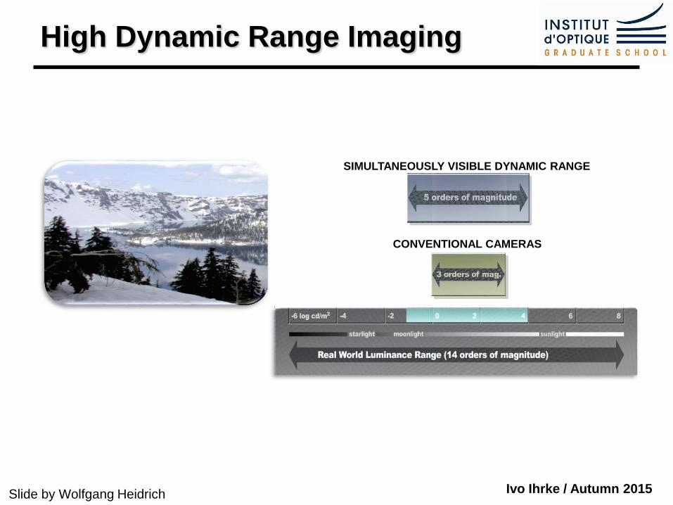
High Dynamic Range Imaging
SIMULTANEOUSLY VISIBLE DYNAMIC RANGE
CONVENTIONAL CAMERAS
Slide by Wolfgang Heidrich
Ivo Ihrke / Autumn 2015
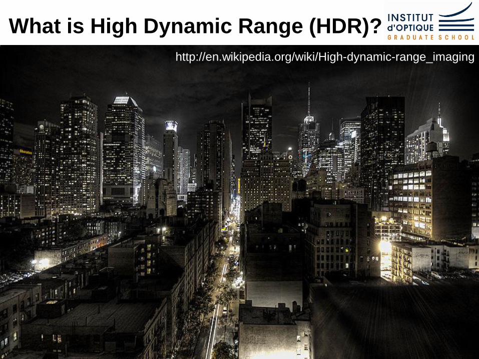
What is High Dynamic Range (HDR)?
http://en.wikipedia.org/wiki/High-dynamic-range_imaging
Ivo Ihrke / Autumn 2015
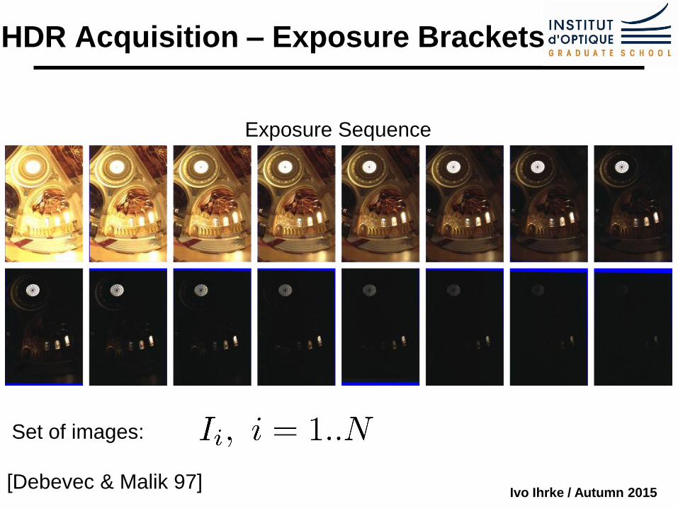
HDR Acquisition – Exposure Brackets
[Debevec & Malik 97]
Exposure Sequence
Set of images:
Ivo Ihrke / Autumn 2015
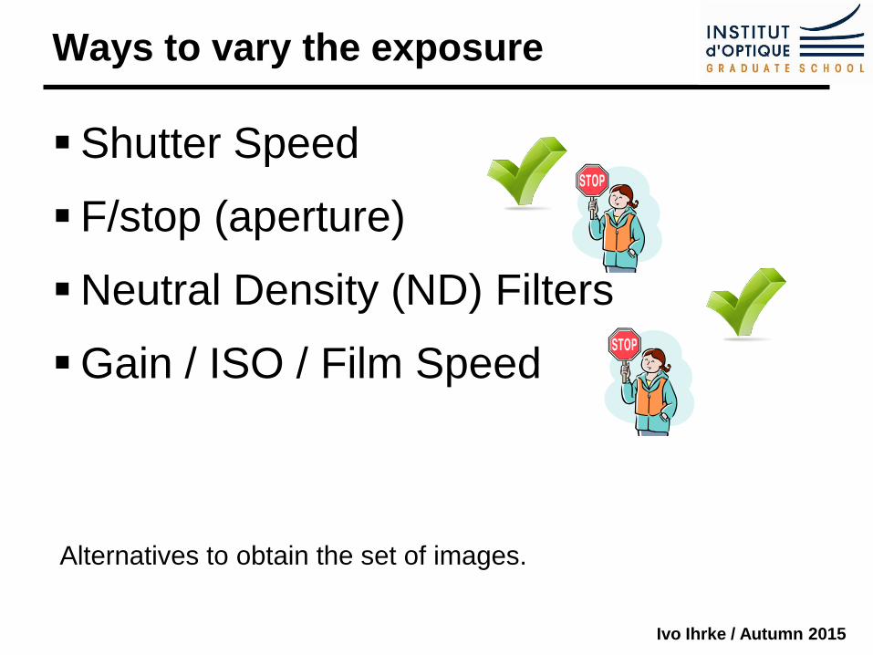
Shutter Speed
F/stop (aperture)
Neutral Density (ND) Filters
Gain / ISO / Film Speed
(DOF)
(noise)
Ways to vary the exposure
Alternatives to obtain the set of images.
Ivo Ihrke / Autumn 2015
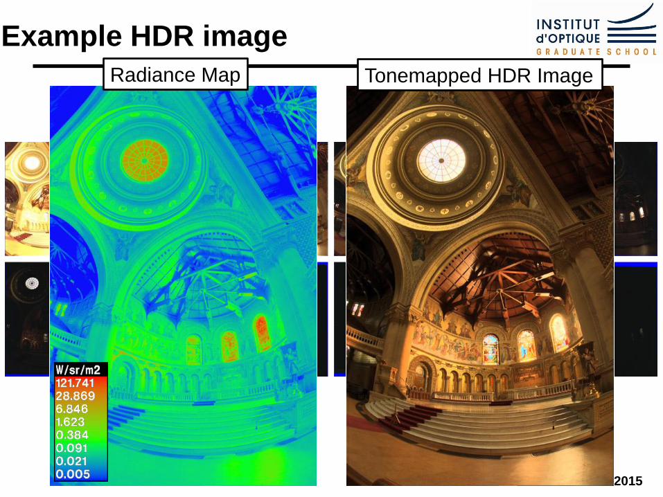
Example HDR image
Radiance Map Tonemapped HDR Image
Ivo Ihrke / Autumn 2015
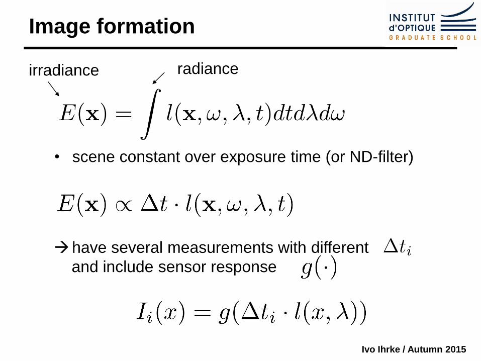
Image formation
• scene constant over exposure time (or ND-filter)
radiance
have several measurements with different
and include sensor response
irradiance
Ivo Ihrke / Autumn 2015
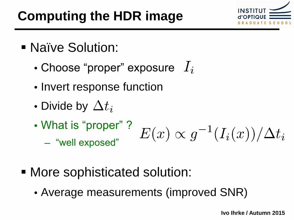
Computing the HDR image
Naïve Solution:
Choose “proper” exposure
Invert response function
Divide by
What is “proper” ?
─ “well exposed”
More sophisticated solution:
Average measurements (improved SNR)
Ivo Ihrke / Autumn 2015
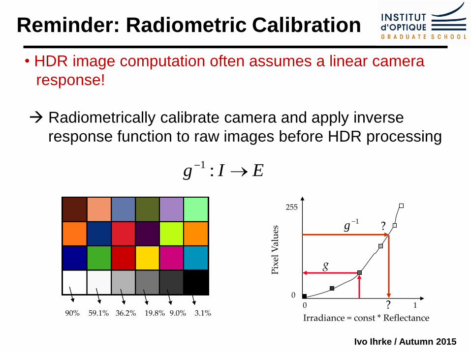
• HDR image computation often assumes a linear camera
response!
Radiometrically calibrate camera and apply inverse
response function to raw images before HDR processing
EIg :1
Irradiance = const * Reflectance
Pix
el V
alu
es
3.1% 9.0% 19.8% 36.2% 59.1% 90%
0
255
0 1
g
?
? 1g
Reminder: Radiometric Calibration
Ivo Ihrke / Autumn 2015
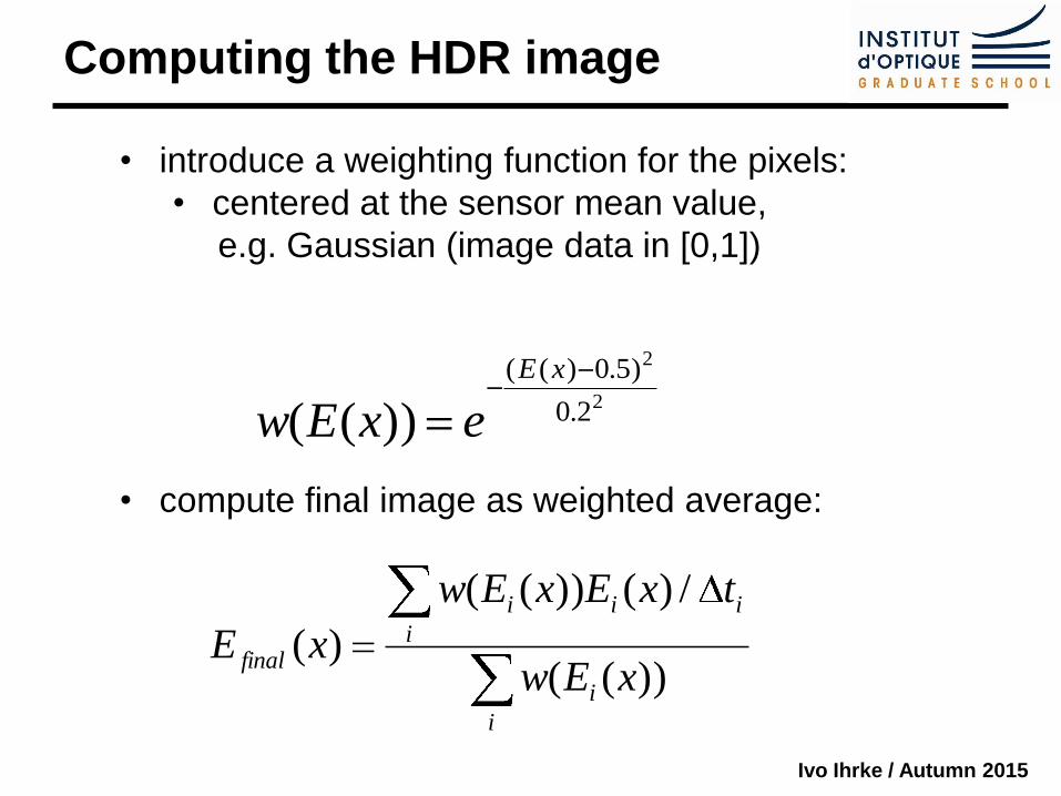
Computing the HDR image
• introduce a weighting function for the pixels:
• centered at the sensor mean value,
e.g. Gaussian (image data in [0,1])
• compute final image as weighted average:
2
2
2.0
)5.0)((
))((
xE
exEw
i
i
i
iii
finalxEw
txExEw
xE))((
/)())((
)(
Ivo Ihrke / Autumn 2015
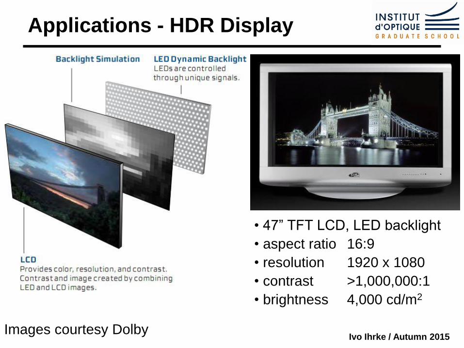
Applications - HDR Display
• 47” TFT LCD, LED backlight
• aspect ratio 16:9
• resolution 1920 x 1080
• contrast >1,000,000:1
• brightness 4,000 cd/m2
Images courtesy Dolby
Ivo Ihrke / Autumn 2015
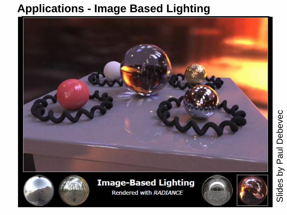
Applications - Image Based Lighting
Slid
es b
y P
aul D
ebe
vec

Ivo Ihrke / Autumn 2015
Ivo Ihrke / Autumn 2015
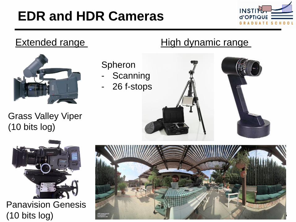
EDR and HDR Cameras
Grass Valley Viper
(10 bits log)
Panavision Genesis
(10 bits log)
Spheron
- Scanning
- 26 f-stops
Extended range High dynamic range
Ivo Ihrke / Autumn 2015
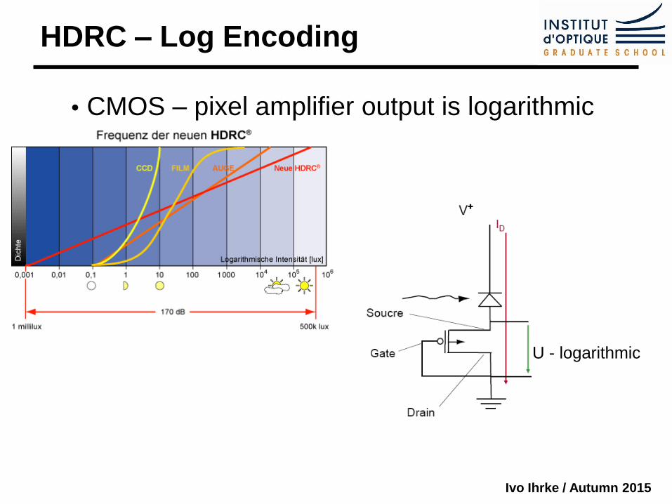
HDRC – Log Encoding
CMOS – pixel amplifier output is logarithmic
U - logarithmic
Ivo Ihrke / Autumn 2015
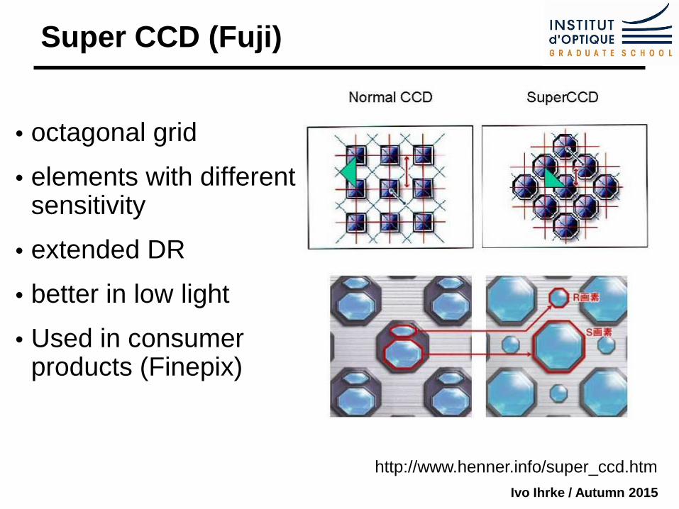
Super CCD (Fuji)
octagonal grid
elements with different sensitivity
extended DR
better in low light
Used in consumer products (Finepix)
http://www.henner.info/super_ccd.htm
Ivo Ihrke / Autumn 2015
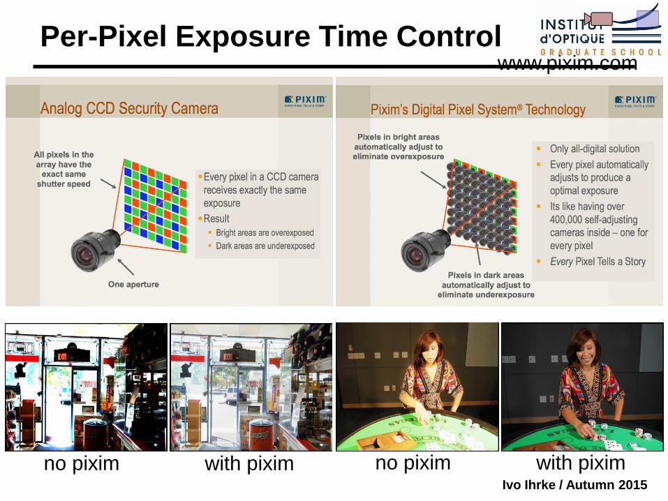
Per-Pixel Exposure Time Control www.pixim.com
no pixim with pixim no pixim with pixim
Ivo Ihrke / Autumn 2015
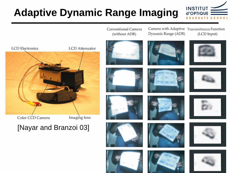
Adaptive Dynamic Range Imaging
[Nayar and Branzoi 03]
Ivo Ihrke / Autumn 2015
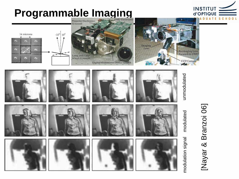
Programmable Imaging
[Nayar
& B
ranzoi 06
]
un
mo
du
late
d
mo
du
late
d
mo
du
latio
n s
ign
al
Ivo Ihrke / Autumn 2015
HDR with Standard Sensors
HDRI with Standard Sensors
Trading for Temporal Resolution
Trading for Spatial Resolution
Multiple Sensors
Generalized Encodings
Ivo Ihrke / Autumn 2015
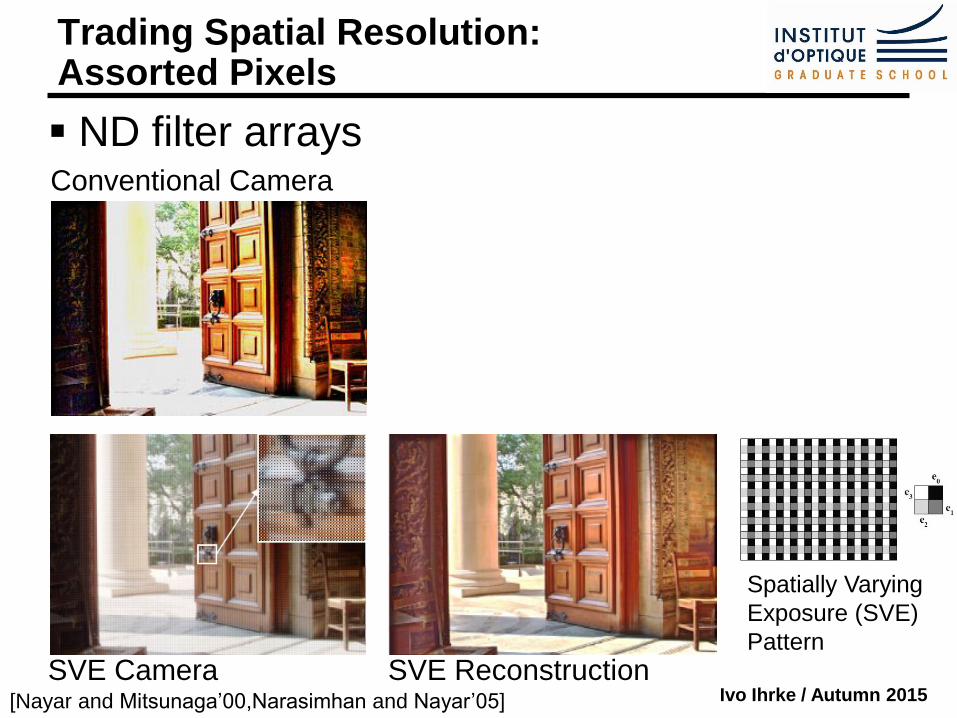
Trading Spatial Resolution: Assorted Pixels
ND filter arrays Conventional Camera
SVE Camera SVE Reconstruction [Nayar and Mitsunaga’00,Narasimhan and Nayar’05]
Spatially Varying
Exposure (SVE)
Pattern
Ivo Ihrke / Autumn 2015
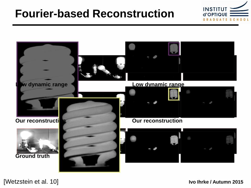
Fourier-based Reconstruction
Low dynamic range
Our reconstruction
Ground truth
Low dynamic range
Our reconstruction
Ground truth
[Wetzstein et al. 10]
Ivo Ihrke / Autumn 2015
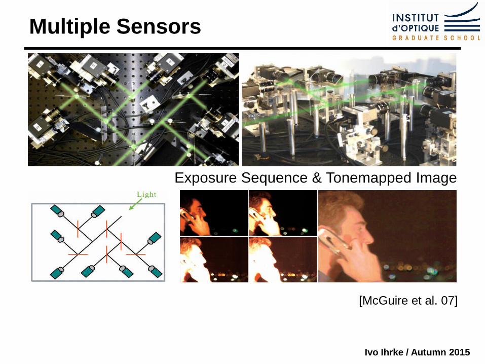
Multiple Sensors
[McGuire et al. 07]
Exposure Sequence & Tonemapped Image
Ivo Ihrke / Autumn 2015
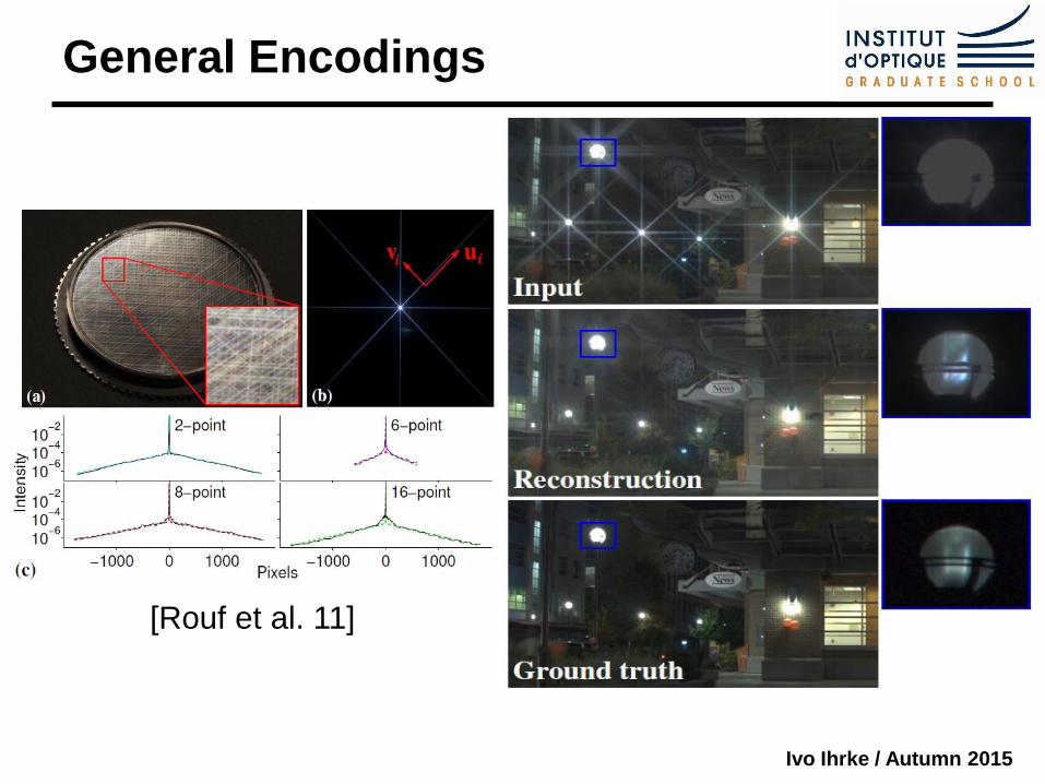
General Encodings
[Rouf et al. 11]
Ivo Ihrke / Autumn 2015
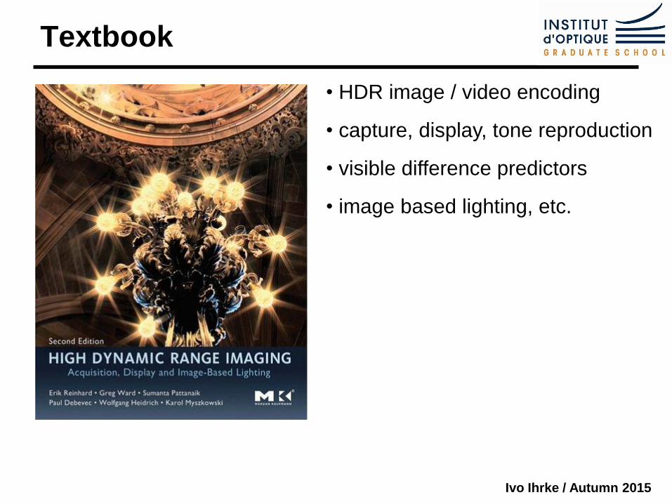
Textbook
• HDR image / video encoding
• capture, display, tone reproduction
• visible difference predictors
• image based lighting, etc.

Ivo Ihrke / Autumn 2015
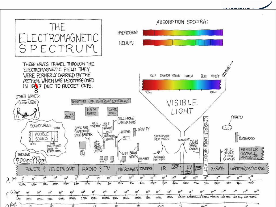
Spectral Imaging
Ivo Ihrke / Autumn 2015
8
Ivo Ihrke / Autumn 2015
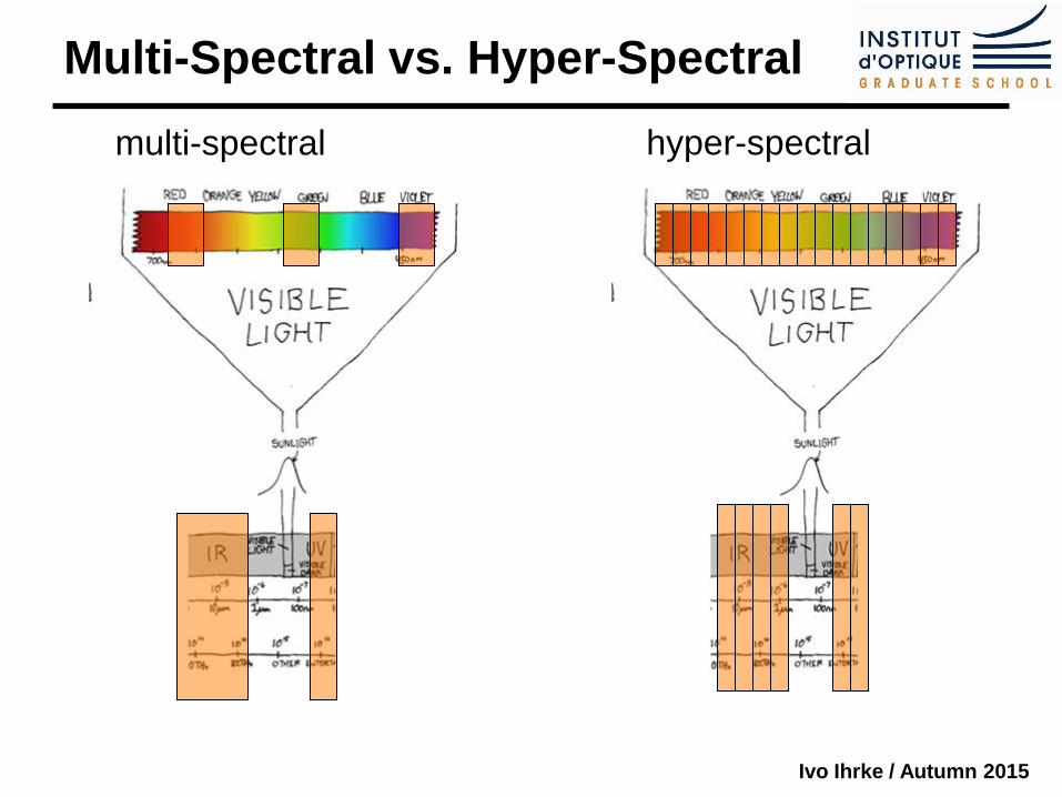
Multi-Spectral vs. Hyper-Spectral
multi-spectral hyper-spectral
Ivo Ihrke / Autumn 2015
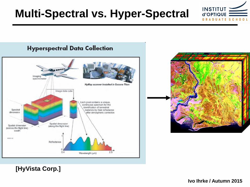
Multi-Spectral vs. Hyper-Spectral
[HyVista Corp.]
Ivo Ihrke / Autumn 2015
Single Pixel Spectrometers
Ivo Ihrke / Autumn 2015
Ivo Ihrke / Autumn 2015
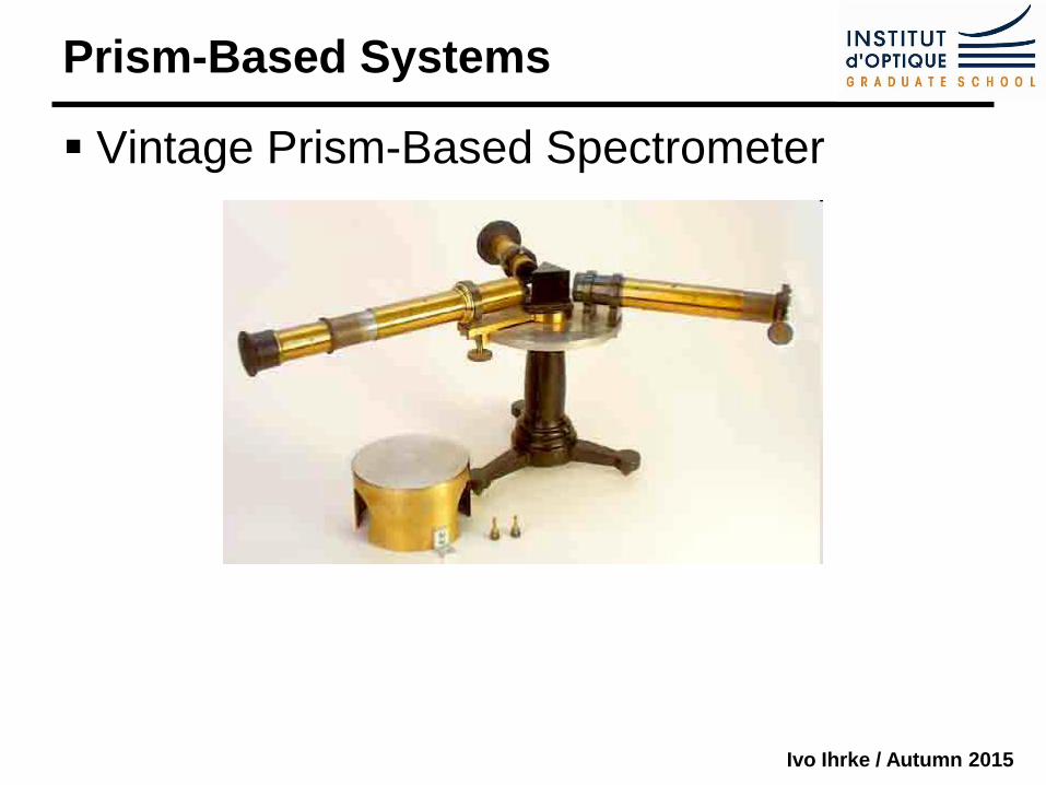
Prism-Based Systems
Vintage Prism-Based Spectrometer
Ivo Ihrke / Autumn 2015
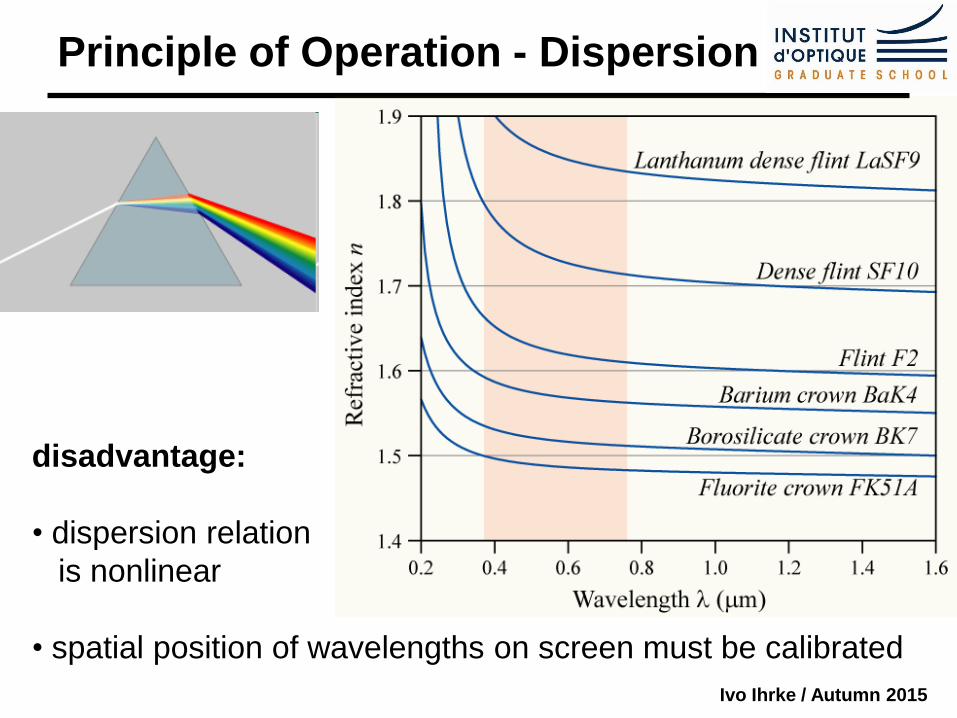
Principle of Operation - Dispersion
disadvantage:
• dispersion relation
is nonlinear
• spatial position of wavelengths on screen must be calibrated
Ivo Ihrke / Autumn 2015
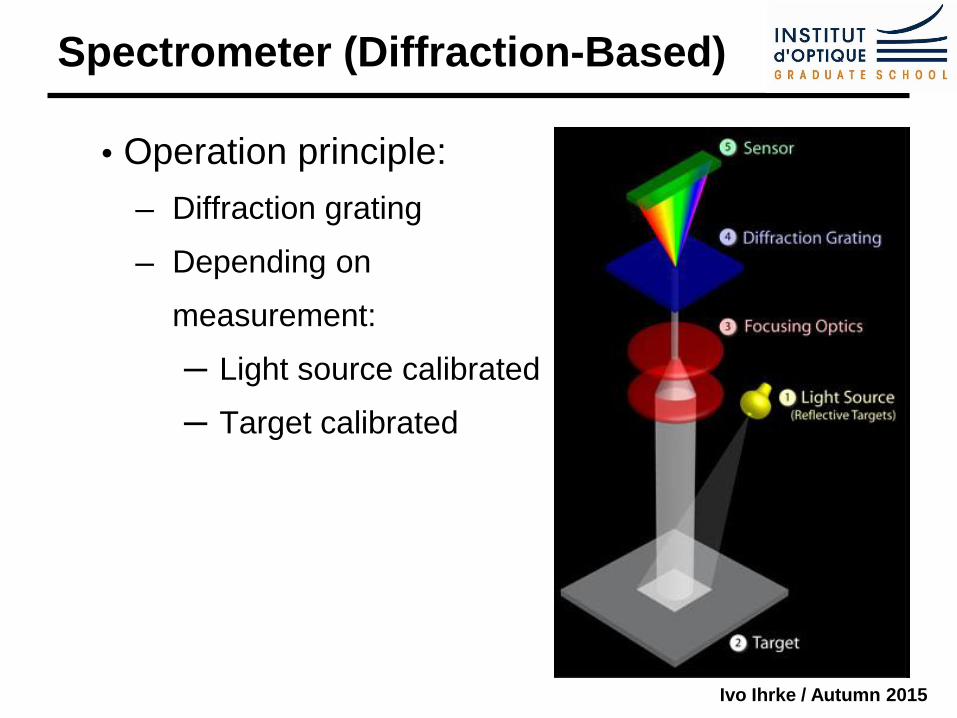
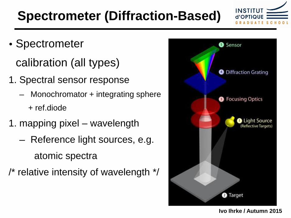
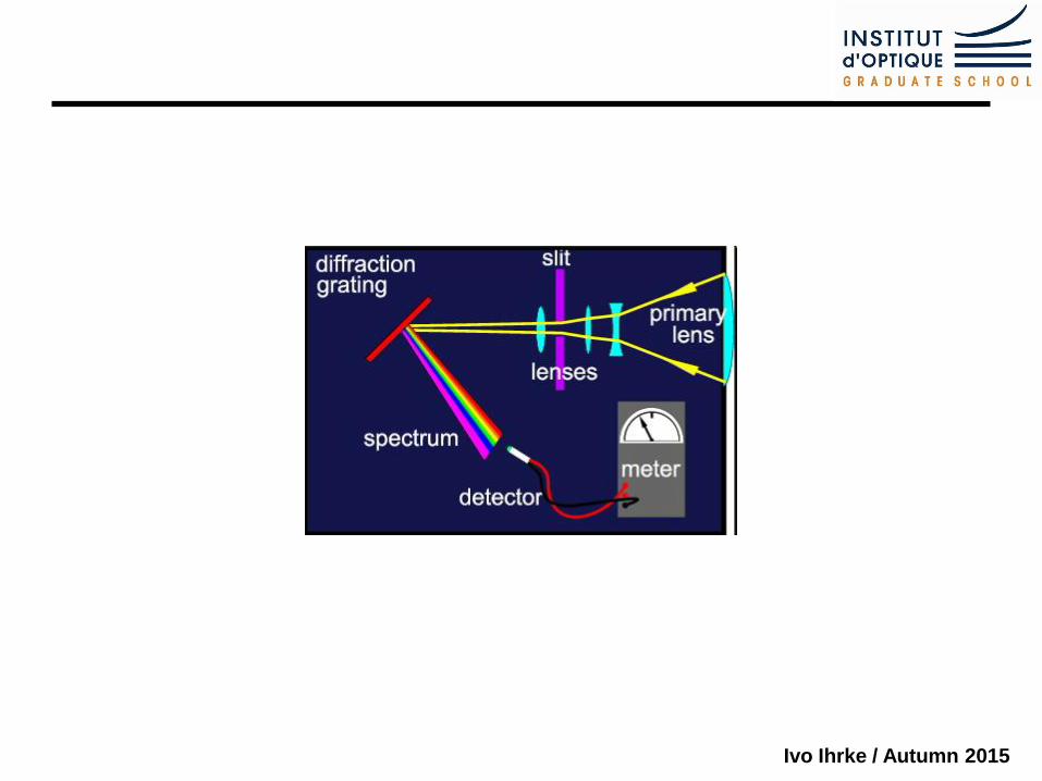
Spectrometer (Diffraction-Based)
Operation principle:
─ Diffraction grating
─ Depending on
measurement:
─ Light source calibrated
─ Target calibrated
Ivo Ihrke / Autumn 2015
Spectrometer (Diffraction-Based)
Spectrometer
calibration (all types)
1. Spectral sensor response
─ Monochromator + integrating sphere
+ ref.diode
1. mapping pixel – wavelength
─ Reference light sources, e.g.
atomic spectra
/* relative intensity of wavelength */
Ivo Ihrke / Autumn 2015
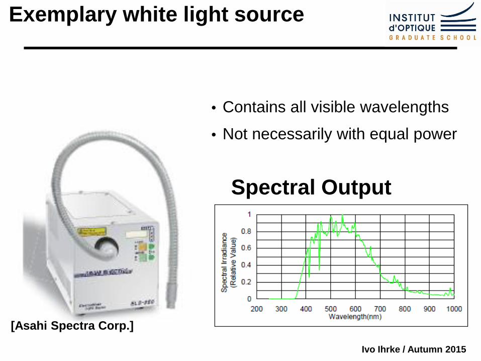
Exemplary white light source
Contains all visible wavelengths
Not necessarily with equal power
[Asahi Spectra Corp.]
Spectral Output
Ivo Ihrke / Autumn 2015
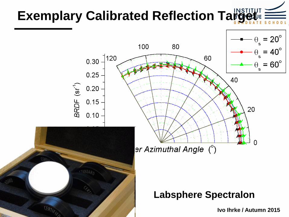
Exemplary Calibrated Reflection Target
Labsphere Spectralon
Ivo Ihrke / Autumn 2015
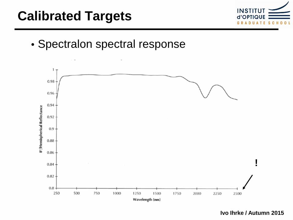
Calibrated Targets
Spectralon spectral response
!
Ivo Ihrke / Autumn 2015
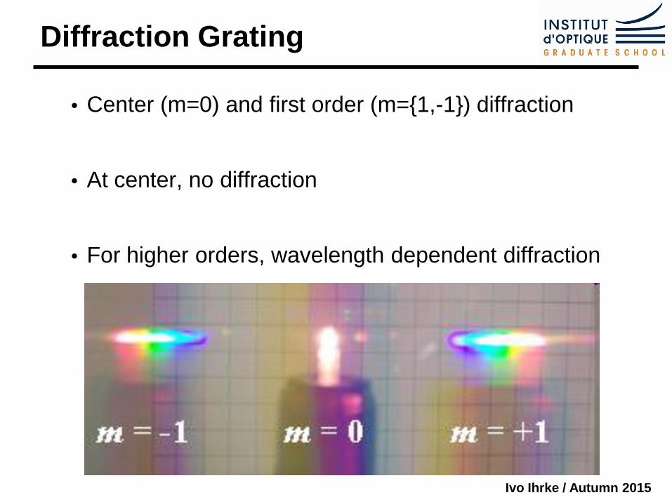
Diffraction Grating
Center (m=0) and first order (m={1,-1}) diffraction
At center, no diffraction
For higher orders, wavelength dependent diffraction
Ivo Ihrke / Autumn 2015
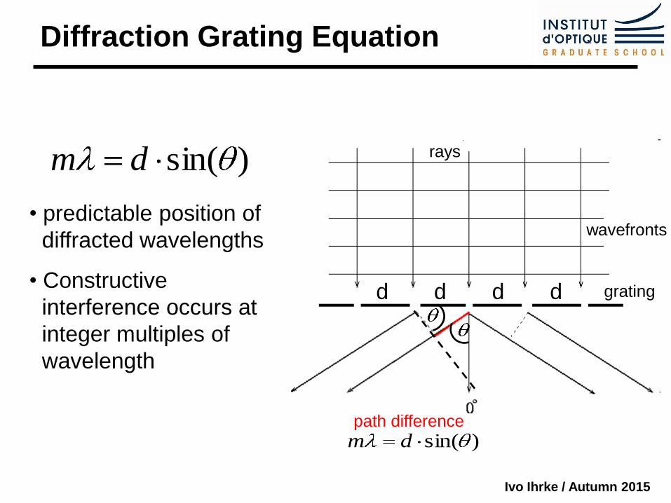
Diffraction Grating Equation
)sin(dm
• predictable position of
diffracted wavelengths
• Constructive
interference occurs at
integer multiples of
wavelength
d d d d
wavefronts
rays
grating
path difference
)sin(dm

Ivo Ihrke / Autumn 2015
Spectral Imaging - Color Filters
Ivo Ihrke / Autumn 2015
James Clerk Maxwell 1831 - 1879
Ivo Ihrke / Autumn 2015
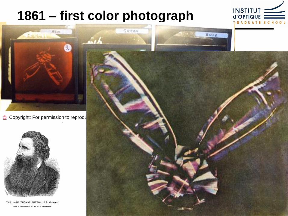
1861 – first color photograph
© Copyright: For permission to reproduce, please contact [email protected]
Ivo Ihrke / Autumn 2015
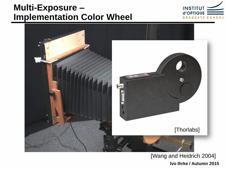
Multi-Exposure – Implementation Color Wheel
[Wang and Heidrich 2004]
[Thorlabs]
Ivo Ihrke / Autumn 2015
Imaging through Color Filters Theory
Ivo Ihrke / Autumn 2015
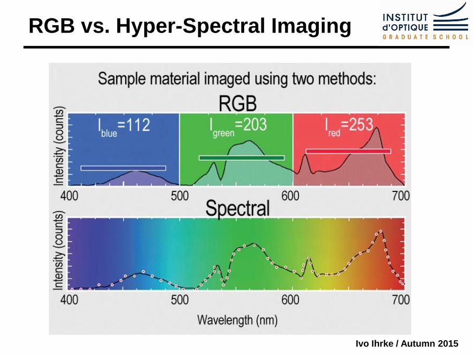
RGB vs. Hyper-Spectral Imaging
Ivo Ihrke / Autumn 2015
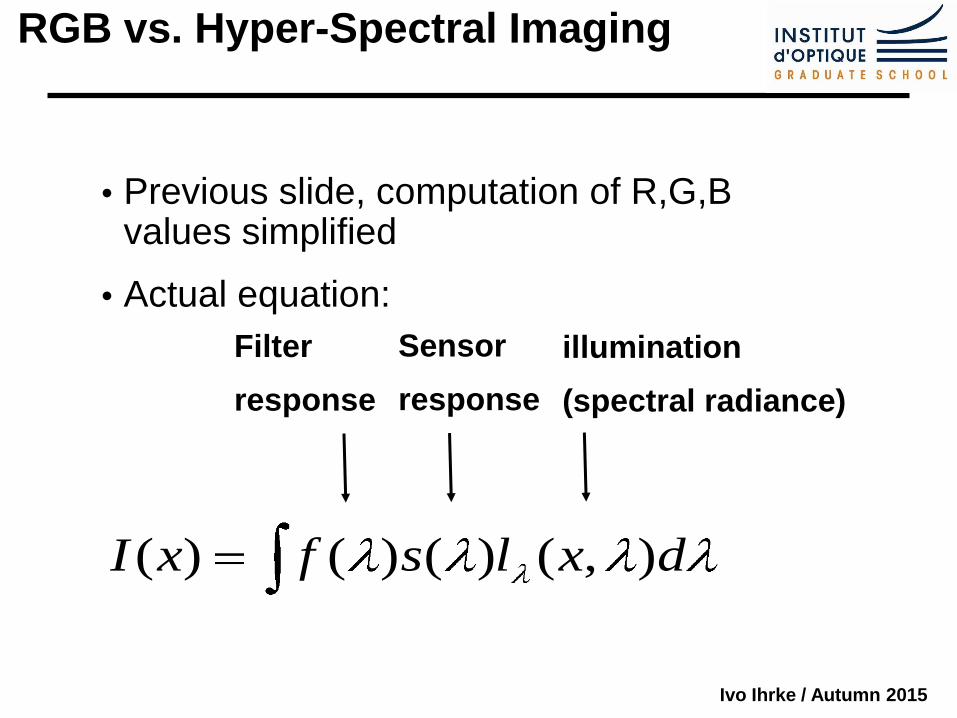
RGB vs. Hyper-Spectral Imaging
Previous slide, computation of R,G,B values simplified
Actual equation:
dxlsfxI ),()()()(
Filter
response
Sensor
response
illumination
(spectral radiance)
Ivo Ihrke / Autumn 2015
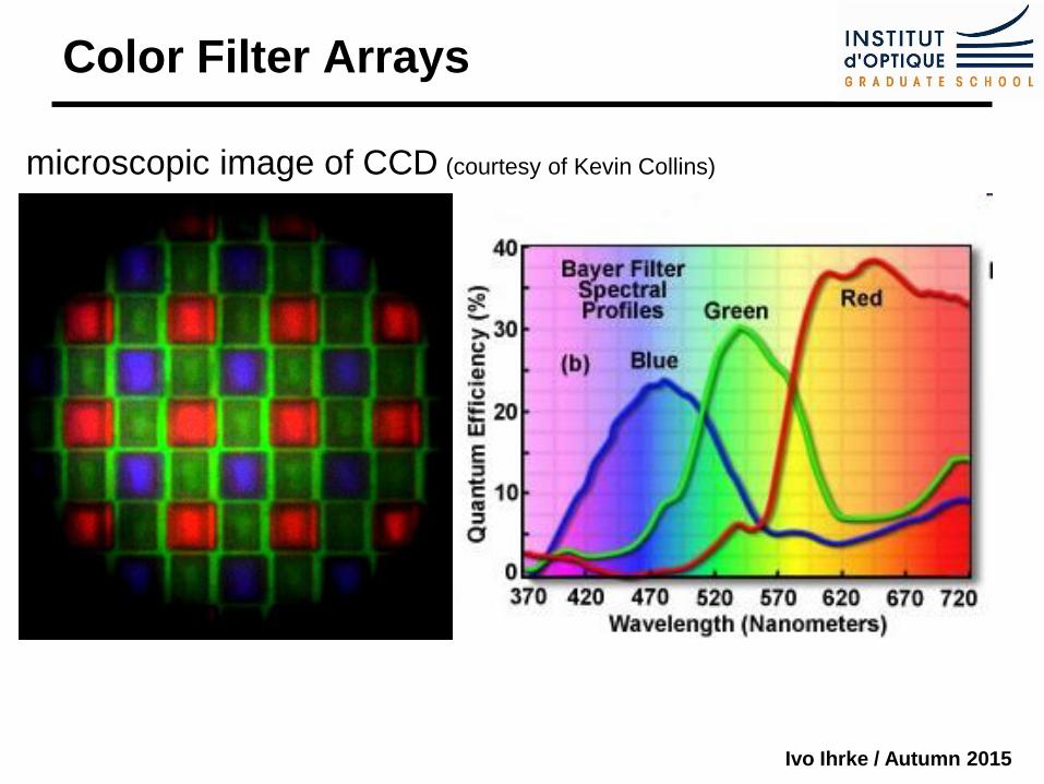
Color Filter Arrays
microscopic image of CCD (courtesy of Kevin Collins)
Ivo Ihrke / Autumn 2015
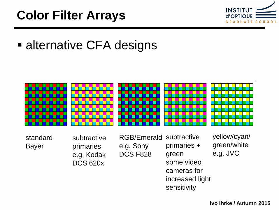
Color Filter Arrays
alternative CFA designs
standard
Bayer subtractive
primaries
e.g. Kodak
DCS 620x
RGB/Emerald
e.g. Sony
DCS F828
subtractive
primaries +
green
some video
cameras for
increased light
sensitivity
yellow/cyan/
green/white
e.g. JVC
Ivo Ihrke / Autumn 2015
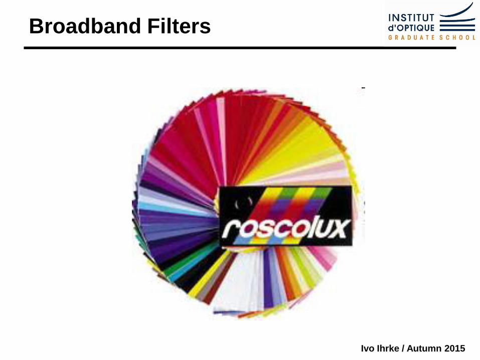
Broadband Filters
Ivo Ihrke / Autumn 2015
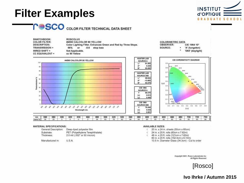
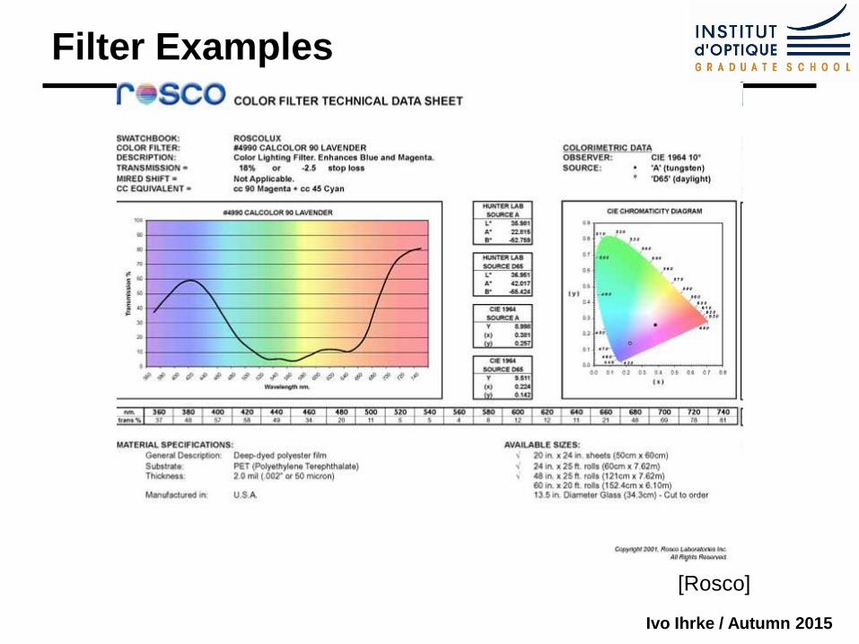
Filter Examples
[Rosco]
Ivo Ihrke / Autumn 2015
Filter Examples
[Rosco]
Ivo Ihrke / Autumn 2015
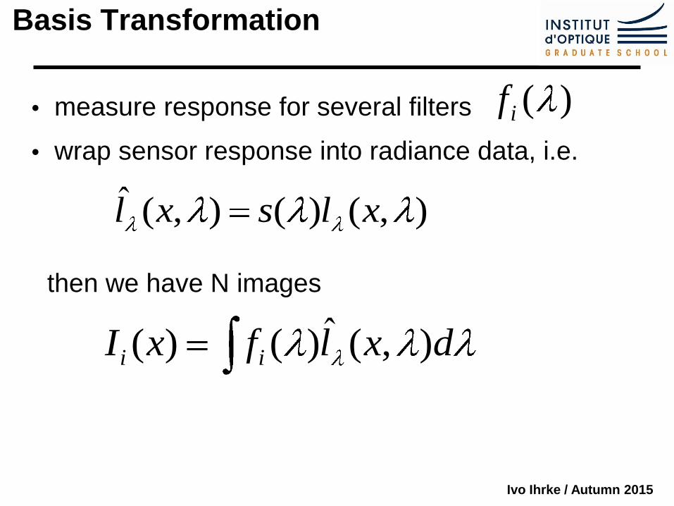
Basis Transformation
measure response for several filters
wrap sensor response into radiance data, i.e.
then we have N images
)(if
),()(),(ˆ xlsxl
dxlfxI ii ),(ˆ)()(
Ivo Ihrke / Autumn 2015
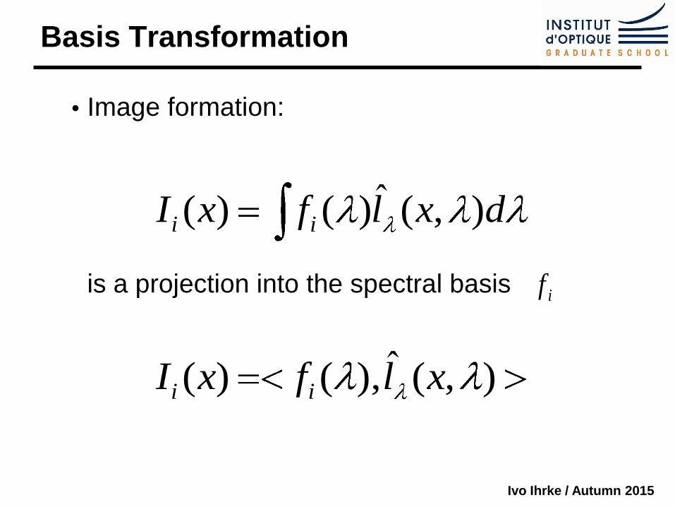
Basis Transformation
Image formation:
is a projection into the spectral basis
dxlfxI ii ),(ˆ)()(
),(ˆ),()( xlfxI ii
if
Ivo Ihrke / Autumn 2015
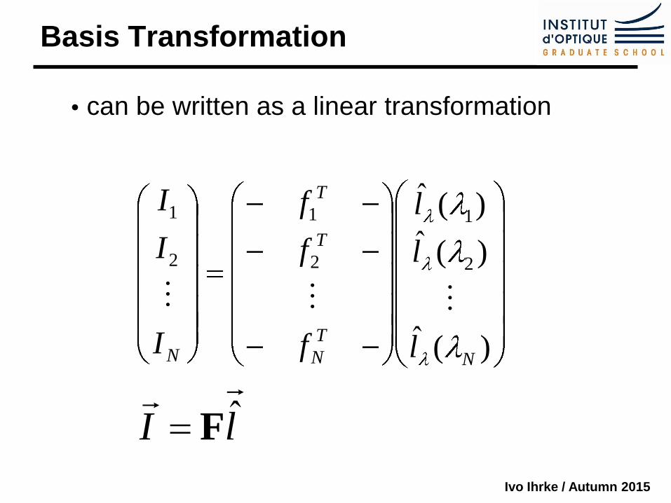
can be written as a linear transformation
Basis Transformation
)(ˆ
)(ˆ
)(ˆ
2
1
2
1
2
1
N
T
N
T
T
N l
l
l
f
f
f
I
I
I
lI
ˆF
Ivo Ihrke / Autumn 2015
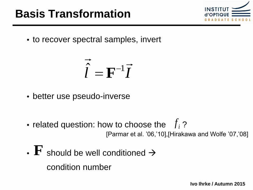
Basis Transformation
to recover spectral samples, invert
better use pseudo-inverse
related question: how to choose the ?
should be well conditioned
condition number
Il
1ˆ F
if
F
[Parmar et al. ’06,’10],[Hirakawa and Wolfe ’07,’08]
Ivo Ihrke / Autumn 2015
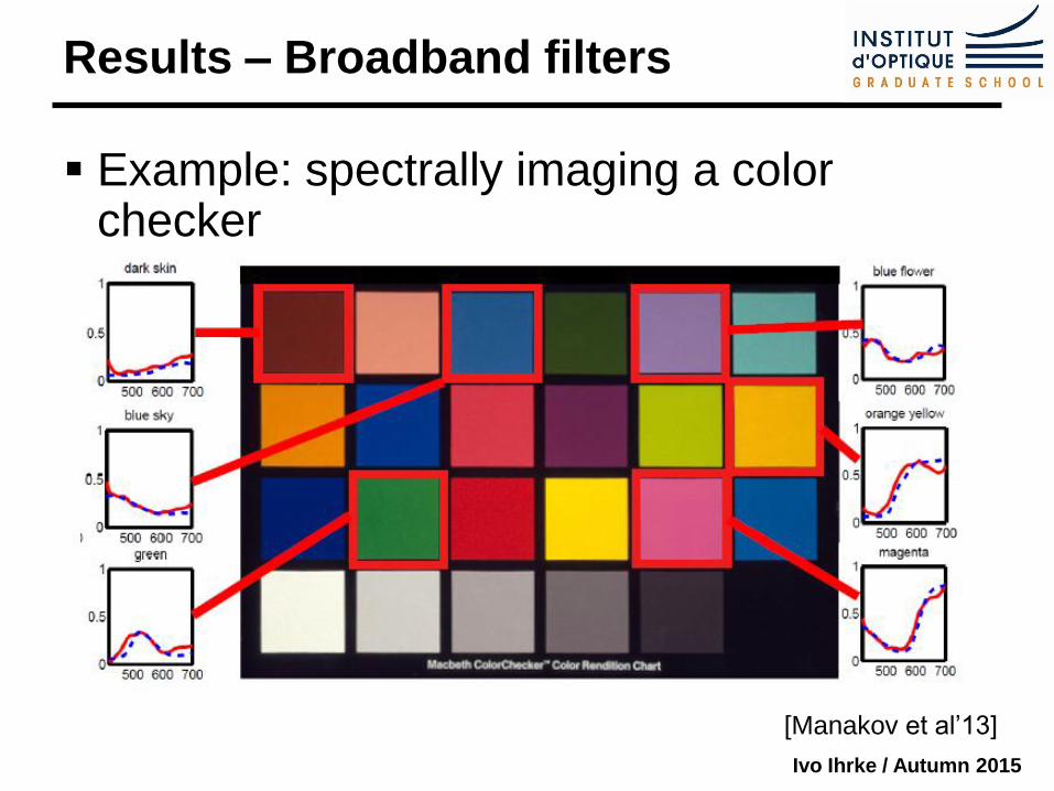
Results – Broadband filters
Example: spectrally imaging a color checker
[Manakov et al’13]
Ivo Ihrke / Autumn 2015
Spectral Imaging - Tunable Filters
Ivo Ihrke / Autumn 2015
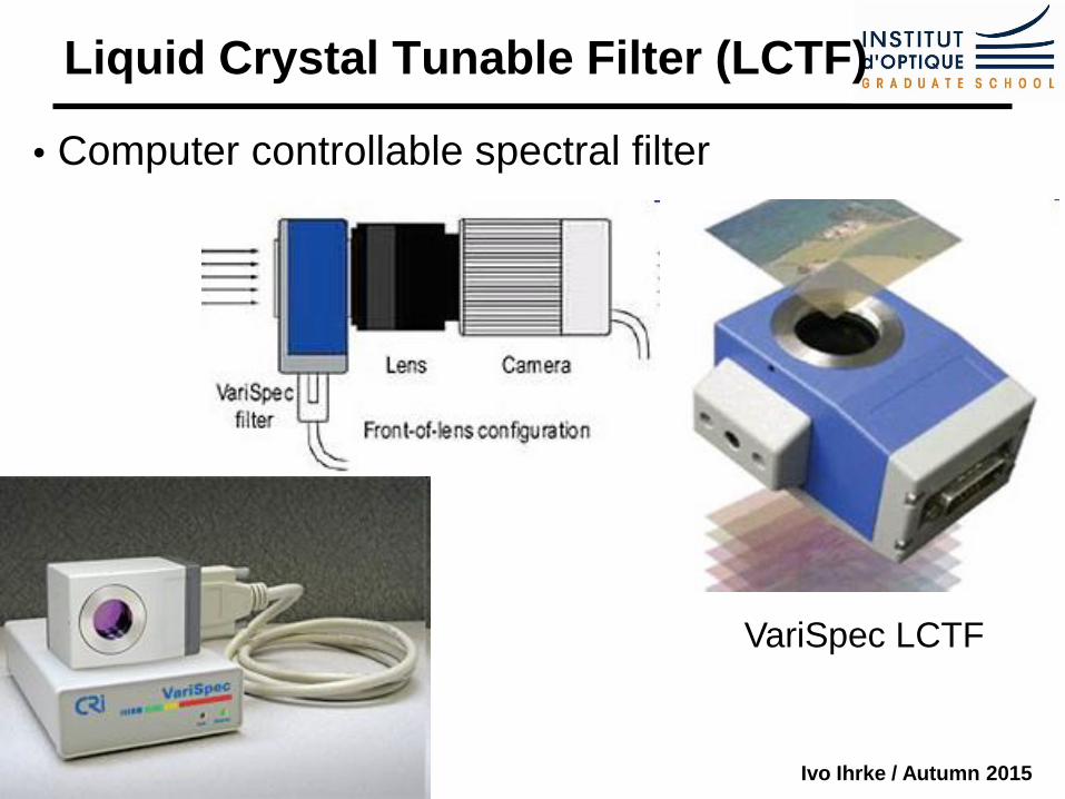
Liquid Crystal Tunable Filter (LCTF)
Computer controllable spectral filter
VariSpec LCTF
Ivo Ihrke / Autumn 2015
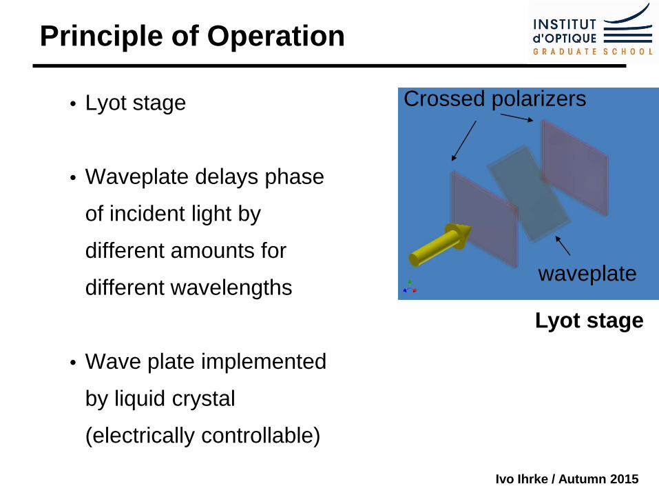
Principle of Operation
Lyot stage
Waveplate delays phase
of incident light by
different amounts for
different wavelengths
Wave plate implemented
by liquid crystal
(electrically controllable)
Lyot stage
Crossed polarizers
waveplate
Ivo Ihrke / Autumn 2015
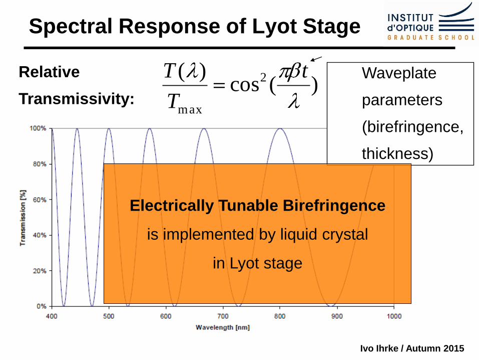
Spectral Response of Lyot Stage
)(cos)( 2
max
t
T
TRelative
Transmissivity:
Waveplate
parameters
(birefringence,
thickness)
Electrically Tunable Birefringence
is implemented by liquid crystal
in Lyot stage
Ivo Ihrke / Autumn 2015
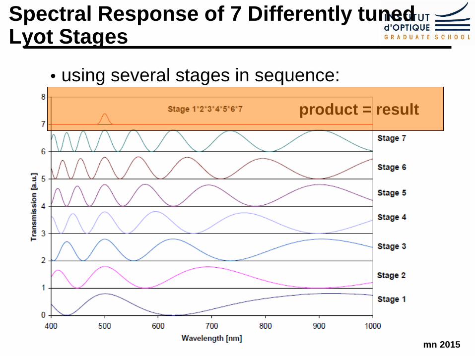
Spectral Response of 7 Differently tuned Lyot Stages
using several stages in sequence:
product = result
Ivo Ihrke / Autumn 2015
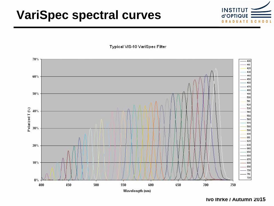
VariSpec spectral curves
Ivo Ihrke / Autumn 2015
Scanning Spectrometers
Ivo Ihrke / Autumn 2015
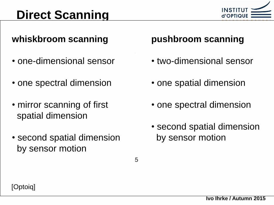
Direct Scanning
pushbroom scanning
• two-dimensional sensor
• one spatial dimension
• one spectral dimension
• second spatial dimension
by sensor motion
whiskbroom scanning
• one-dimensional sensor
• one spectral dimension
• mirror scanning of first
spatial dimension
• second spatial dimension
by sensor motion
[Optoiq]
Ivo Ihrke / Autumn 2015
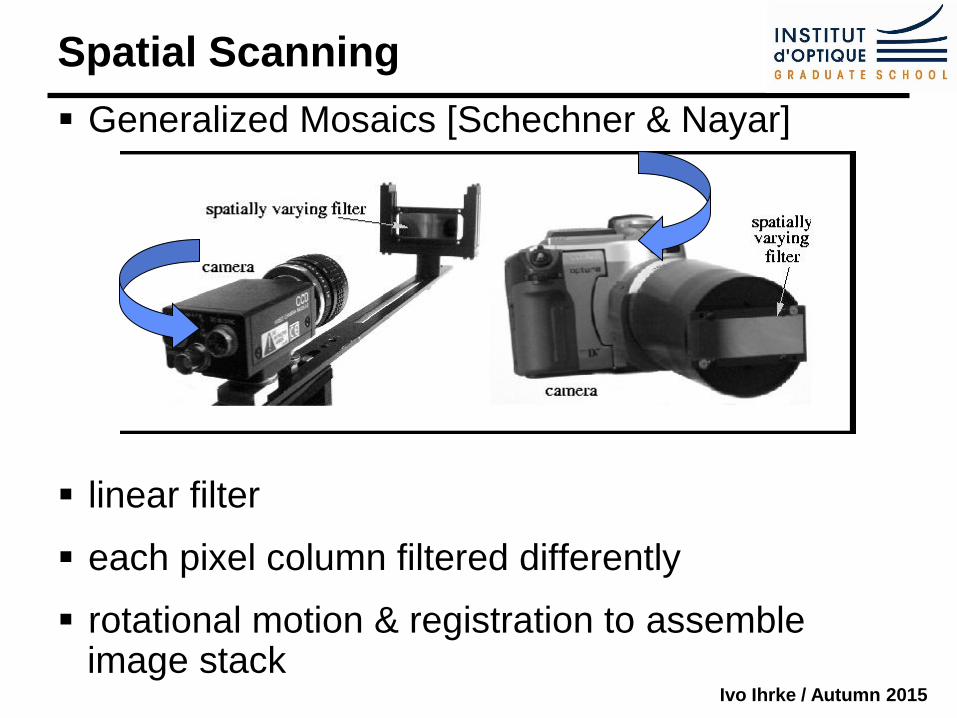
Spatial Scanning
Generalized Mosaics [Schechner & Nayar]
linear filter
each pixel column filtered differently
rotational motion & registration to assemble image stack
Ivo Ihrke / Autumn 2015
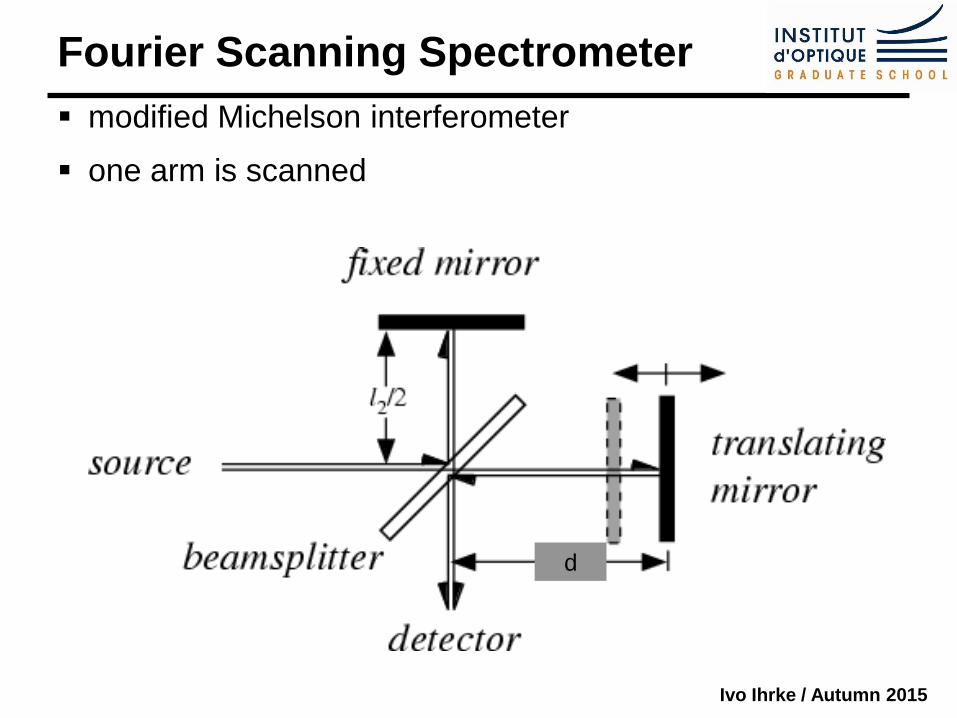
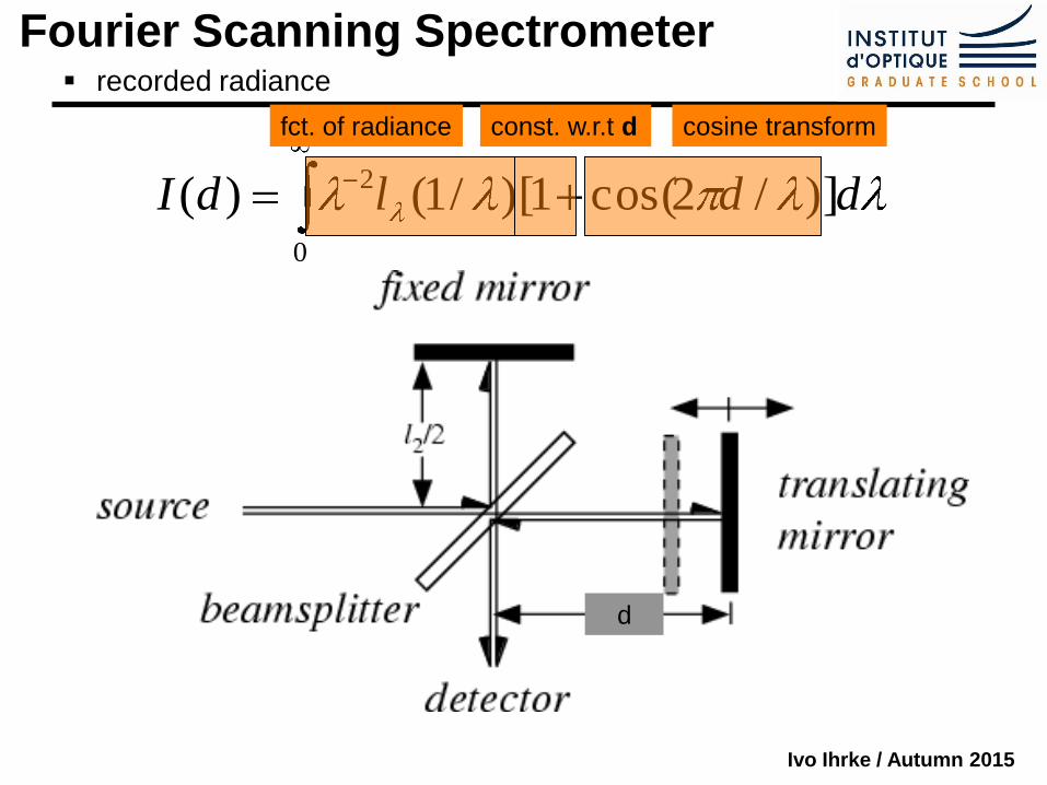
Fourier Scanning Spectrometer
modified Michelson interferometer
one arm is scanned
d
Ivo Ihrke / Autumn 2015
Fourier Scanning Spectrometer recorded radiance
d
ddldI )]/2cos(1)[/1()(0
2
const. w.r.t d cosine transform fct. of radiance
Ivo Ihrke / Autumn 2015
Snapshot Imaging Spectrometers
Ivo Ihrke / Autumn 2015
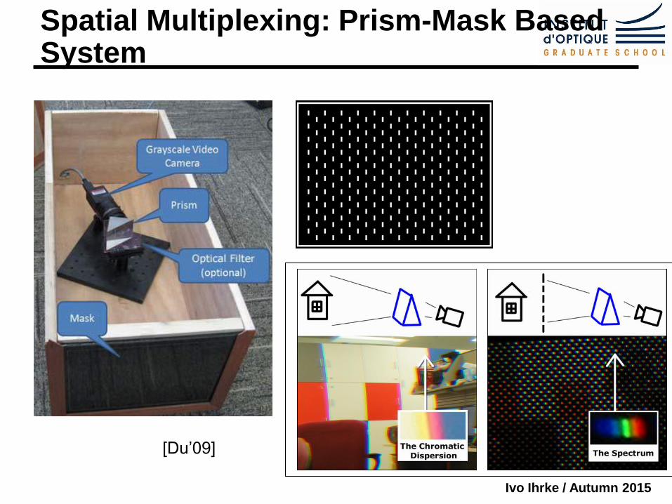
Spatial Multiplexing: Prism-Mask Based System
[Du’09]
Ivo Ihrke / Autumn 2015
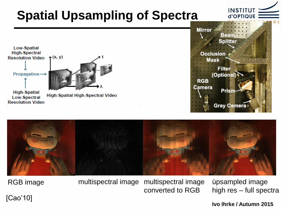
Spatial Upsampling of Spectra
[Cao’10]
RGB image multispectral image multispectral image
converted to RGB
ùpsampled image
high res – full spectra
Ivo Ihrke / Autumn 2015
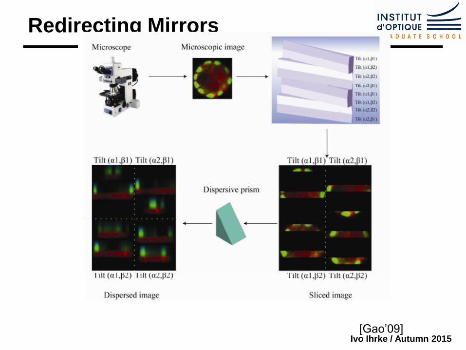
Redirecting Mirrors
[Gao’09]
Ivo Ihrke / Autumn 2015
Computational Spectrometers
Ivo Ihrke / Autumn 2015
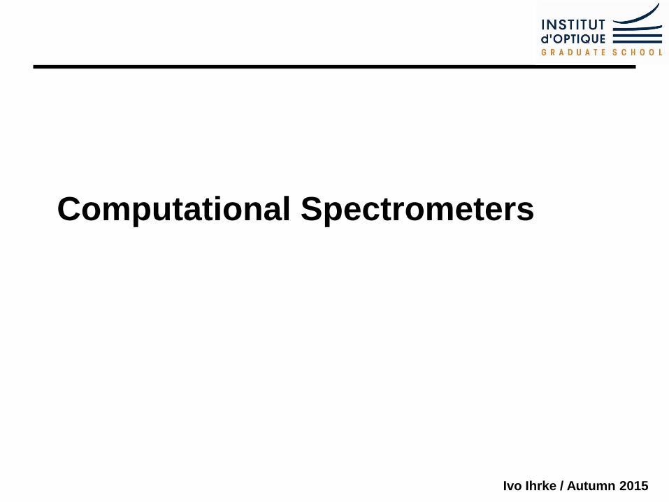
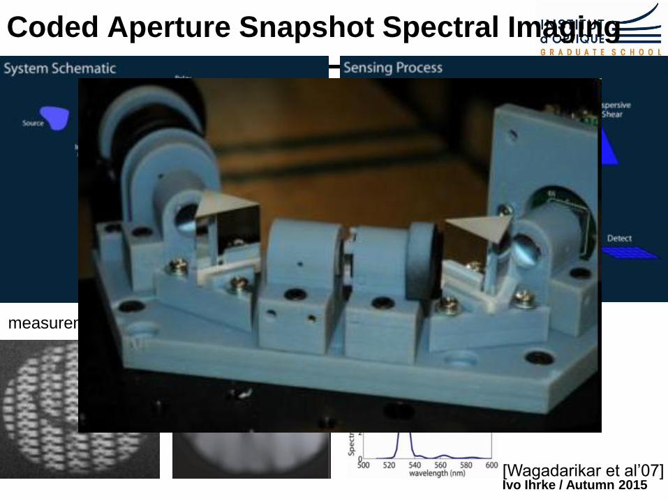
[Wagadarikar et al’07]
measurement CS reconstruction spectrum in center of image
Coded Aperture Snapshot Spectral Imaging
Ivo Ihrke / Autumn 2015
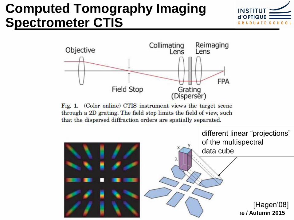
Computed Tomography Imaging Spectrometer CTIS
[Hagen’08]
different linear “projections”
of the multispectral
data cube

Ivo Ihrke / Autumn 2015
Applications
Ivo Ihrke / Autumn 2015
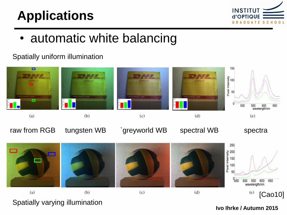
Applications
• automatic white balancing
Spatially uniform illumination
[Cao10] Spatially varying illumination
raw from RGB tungsten WB `greyworld WB spectral WB spectra
Ivo Ihrke / Autumn 2015
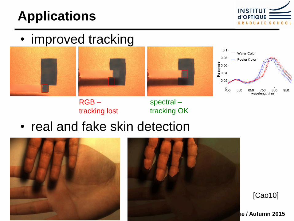
Applications
• improved tracking
• real and fake skin detection
[Cao10]
RGB –
tracking lost
spectral –
tracking OK
Ivo Ihrke / Autumn 2015
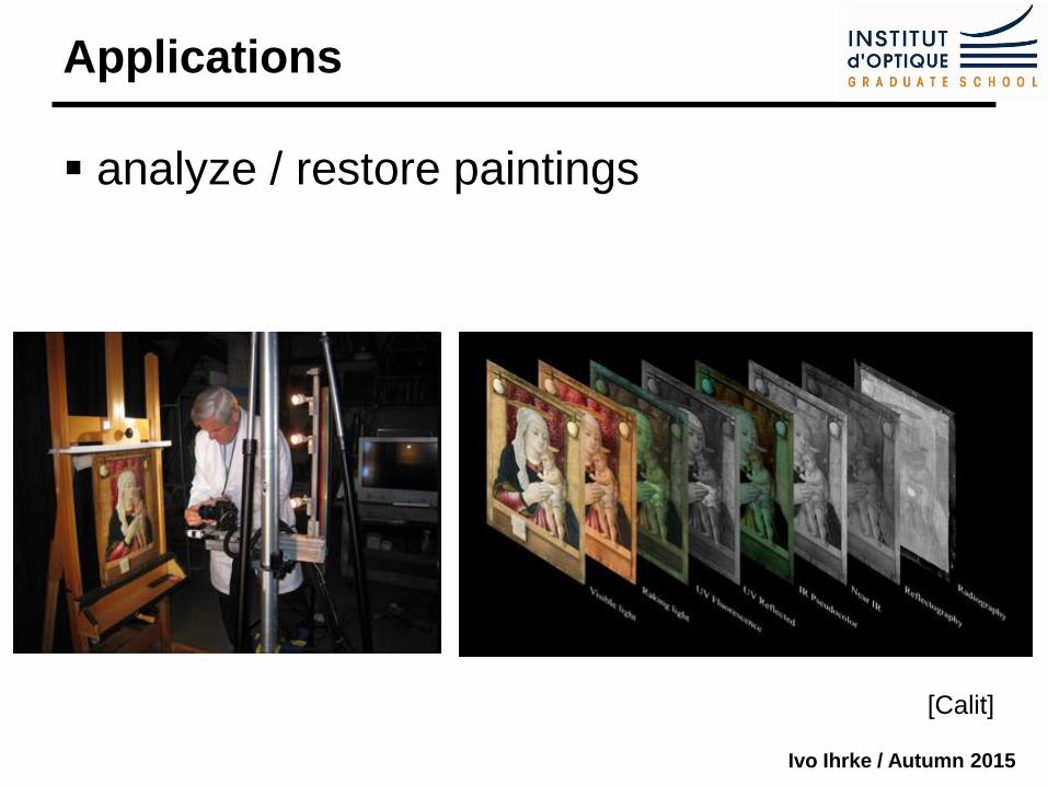
Applications
analyze / restore paintings
[Calit]
Ivo Ihrke / Autumn 2015
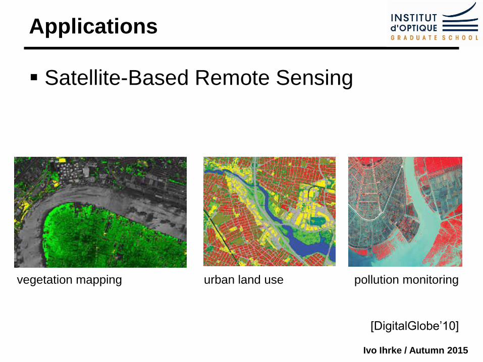
Applications
Satellite-Based Remote Sensing
[DigitalGlobe’10]
vegetation mapping urban land use pollution monitoring

Ivo Ihrke / Autumn 2015
Imaging Polarimetry
Ivo Ihrke / Autumn 2015
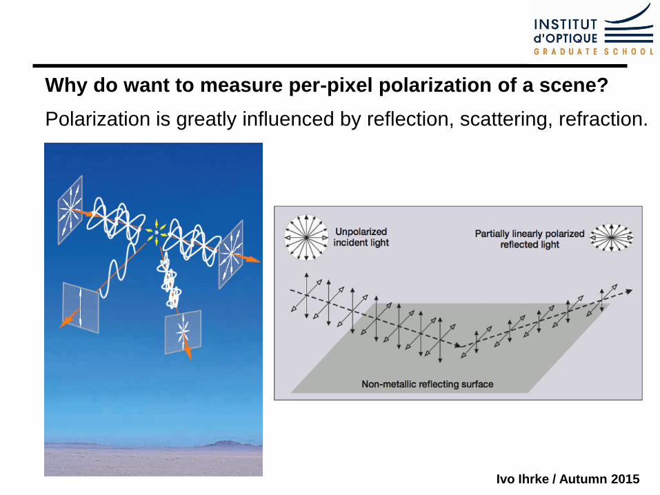
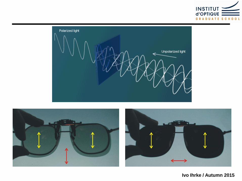
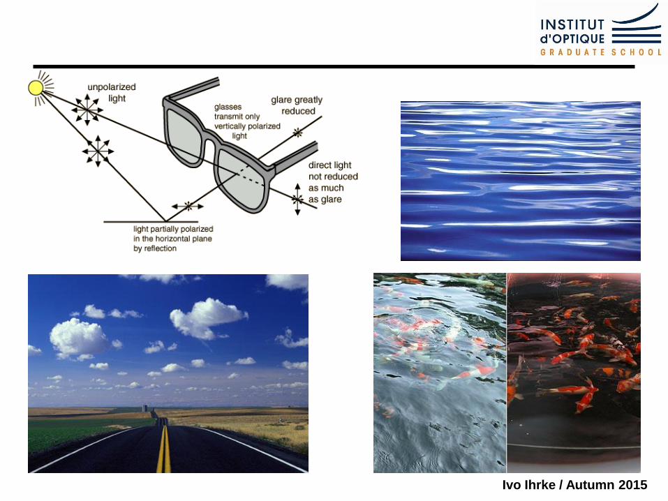
Why do want to measure per-pixel polarization of a scene?
Polarization is greatly influenced by reflection, scattering, refraction.
Ivo Ihrke / Autumn 2015
Ivo Ihrke / Autumn 2015
Ivo Ihrke / Autumn 2015
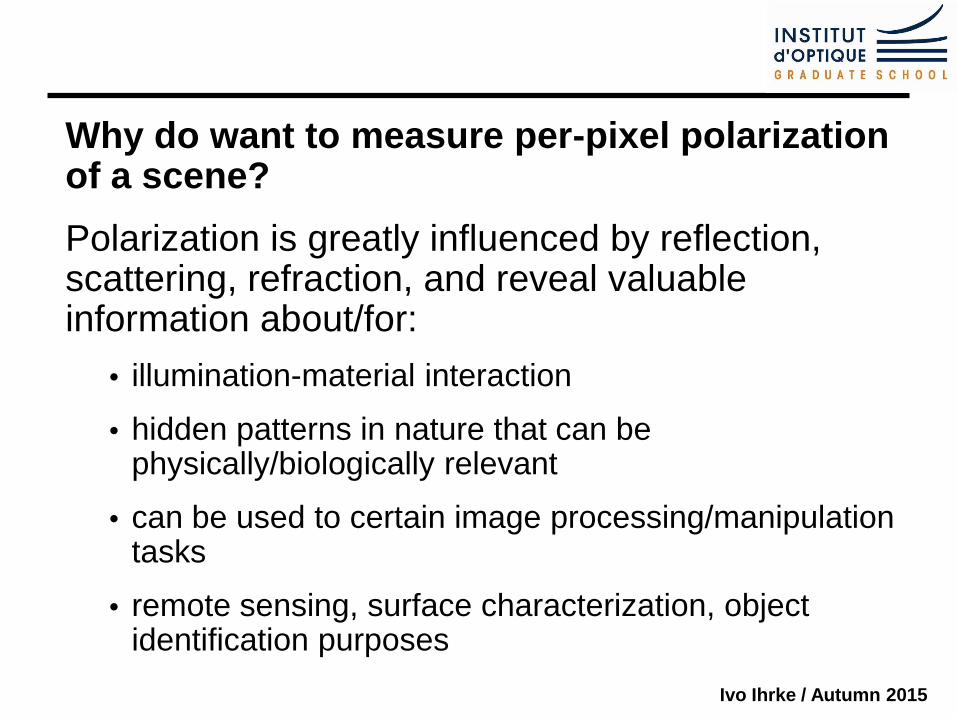
Why do want to measure per-pixel polarization of a scene?
Polarization is greatly influenced by reflection, scattering, refraction, and reveal valuable information about/for:
illumination-material interaction
hidden patterns in nature that can be physically/biologically relevant
can be used to certain image processing/manipulation tasks
remote sensing, surface characterization, object identification purposes
Ivo Ihrke / Autumn 2015
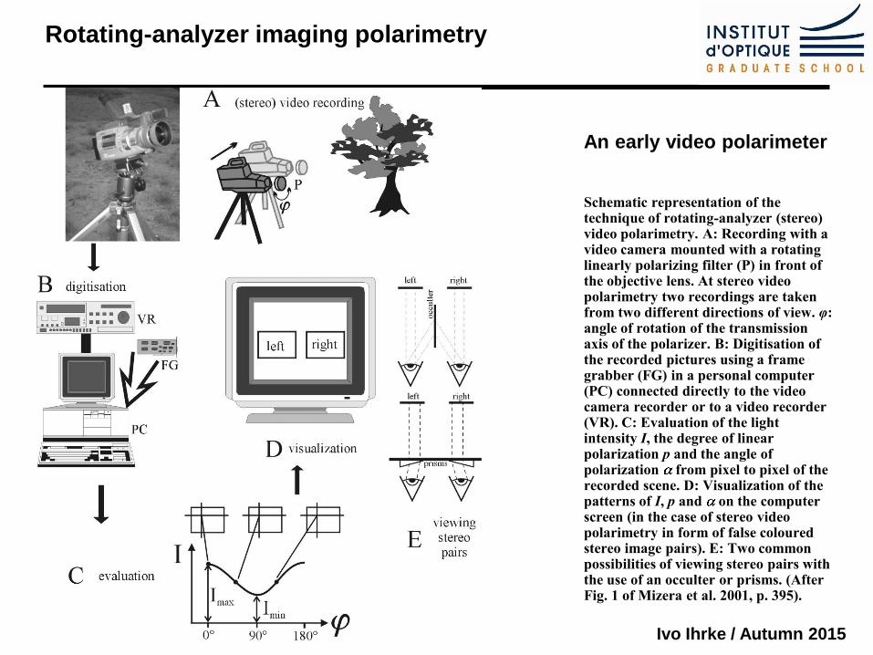
An early video polarimeter Schematic representation of the technique of rotating-analyzer (stereo) video polarimetry. A: Recording with a video camera mounted with a rotating linearly polarizing filter (P) in front of the objective lens. At stereo video polarimetry two recordings are taken from two different directions of view. φ: angle of rotation of the transmission axis of the polarizer. B: Digitisation of the recorded pictures using a frame grabber (FG) in a personal computer (PC) connected directly to the video camera recorder or to a video recorder (VR). C: Evaluation of the light intensity I, the degree of linear polarization p and the angle of polarization from pixel to pixel of the recorded scene. D: Visualization of the patterns of I, p and on the computer screen (in the case of stereo video polarimetry in form of false coloured stereo image pairs). E: Two common possibilities of viewing stereo pairs with the use of an occulter or prisms. (After Fig. 1 of Mizera et al. 2001, p. 395).
Rotating-analyzer imaging polarimetry
Ivo Ihrke / Autumn 2015
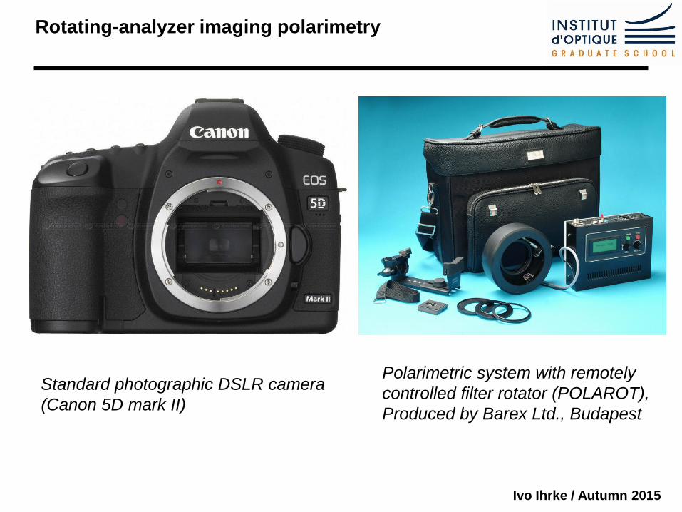
Polarimetric system with remotely
controlled filter rotator (POLAROT),
Produced by Barex Ltd., Budapest
Rotating-analyzer imaging polarimetry
Standard photographic DSLR camera
(Canon 5D mark II)
Ivo Ihrke / Autumn 2015
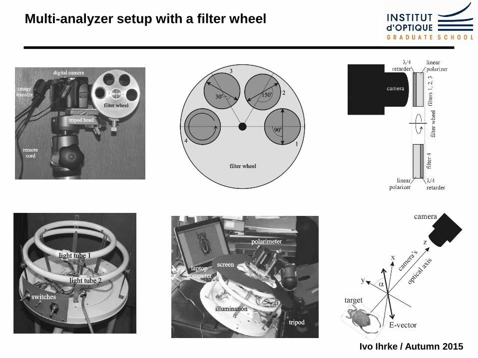
Multi-analyzer setup with a filter wheel
Ivo Ihrke / Autumn 2015
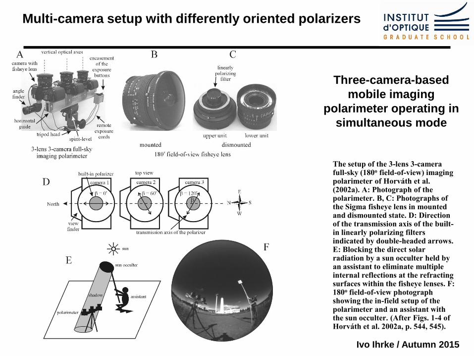
The setup of the 3-lens 3-camera full-sky (180o field-of-view) imaging polarimeter of Horváth et al. (2002a). A: Photograph of the polarimeter. B, C: Photographs of the Sigma fisheye lens in mounted and dismounted state. D: Direction of the transmission axis of the built-in linearly polarizing filters indicated by double-headed arrows. E: Blocking the direct solar radiation by a sun occulter held by an assistant to eliminate multiple internal reflections at the refracting surfaces within the fisheye lenses. F: 180o field-of-view photograph showing the in-field setup of the polarimeter and an assistant with the sun occulter. (After Figs. 1-4 of Horváth et al. 2002a, p. 544, 545).
Three-camera-based
mobile imaging
polarimeter operating in
simultaneous mode
Multi-camera setup with differently oriented polarizers
Ivo Ihrke / Autumn 2015
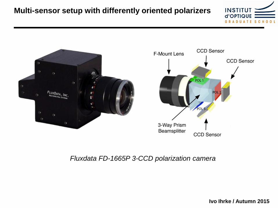
Multi-sensor setup with differently oriented polarizers
Fluxdata FD-1665P 3-CCD polarization camera
Ivo Ihrke / Autumn 2015
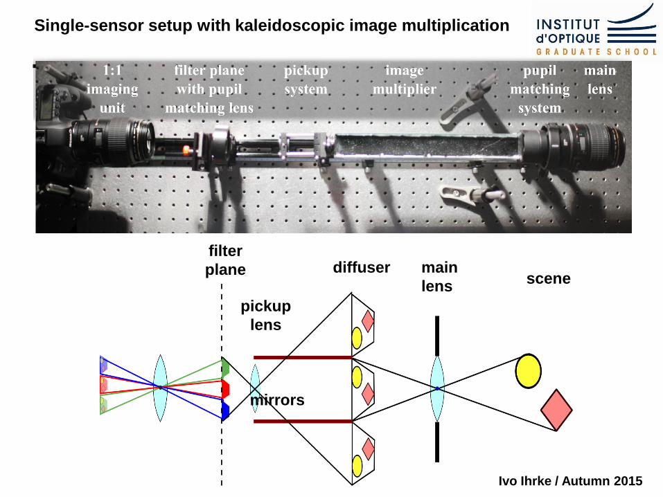
Single-sensor setup with kaleidoscopic image multiplication
main
lens scene
mirrors
pickup
lens
filter
plane diffuser
Ivo Ihrke / Autumn 2015
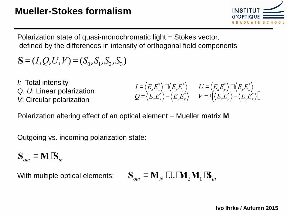
S = (I,Q,U,V ) = (S0,S1,S2,S3)
Mueller-Stokes formalism
Polarization state of quasi-monochromatic light = Stokes vector,
defined by the differences in intensity of orthogonal field components
I: Total intensity
Q, U: Linear polarization
V: Circular polarization
Outgoing vs. incoming polarization state:
Polarization altering effect of an optical element = Mueller matrix M
Sout =M ×Sin
With multiple optical elements: Sout =MN ×...×M2M1 ×Sin
Q = ExEx* - EyEy
*
I = ExEx* + EyEy
* U = ExEy* + EyEx
*
V = i ExEy* - EyEx
*( )
Ivo Ihrke / Autumn 2015
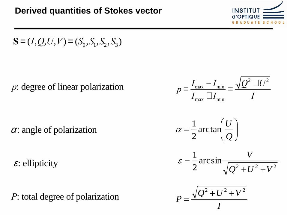
S = (I,Q,U,V ) = (S0,S1,S2,S3)
p: degree of linear polarization
e: ellipticity
a: angle of polarization
P: total degree of polarizationI
VUQP
222
Q
Uarctan
2
1
222arcsin
2
1
VUQ
V
p =Imax - Imin
Imax + Imin
=Q2 +U 2
I
Derived quantities of Stokes vector
Ivo Ihrke / Autumn 2015
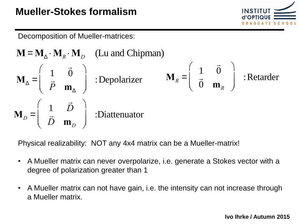
Mueller-Stokes formalism
Decomposition of Mueller-matrices:
MD =1 0
P mD
æ
èçç
ö
ø÷÷
:Depolarizer
M =MD ×MR ×MD (Lu and Chipman)
MR =1 0
0 mR
æ
èçç
ö
ø÷÷
:Retarder
MD =1 D
D mD
æ
èçç
ö
ø÷÷
:Diattenuator
Physical realizability: NOT any 4x4 matrix can be a Mueller-matrix!
• A Mueller matrix can never overpolarize, i.e. generate a Stokes vector with a
degree of polarization greater than 1
• A Mueller matrix can not have gain, i.e. the intensity can not increase through
a Mueller matrix.
Ivo Ihrke / Autumn 2015
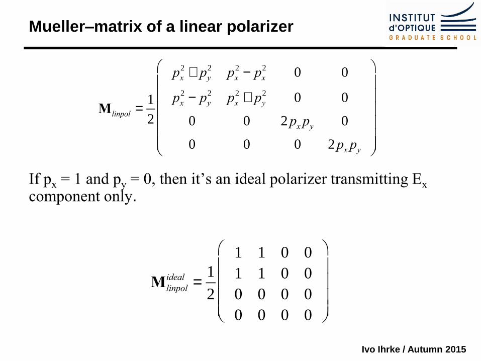
Mueller–matrix of a linear polarizer
If px = 1 and py = 0, then it’s an ideal polarizer transmitting Ex component only.
Mlinpol =1
2
px2 + py
2 px2 - px
2 0 0
px2 - py
2 px2 + py
2 0 0
0 0 2px py 0
0 0 0 2px py
æ
è
çççççç
ö
ø
÷÷÷÷÷÷
Mlinpol
ideal =1
2
1 1 0 0
1 1 0 0
0 0 0 0
0 0 0 0
æ
è
çççç
ö
ø
÷÷÷÷
Ivo Ihrke / Autumn 2015
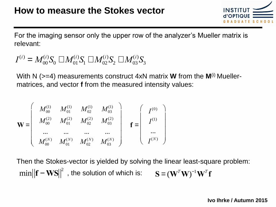
How to measure the Stokes vector
Then the Stokes-vector is yielded by solving the linear least-square problem:
, the solution of which is:
I (i) =M00
(i)S0 +M01
(i)S1 +M02
(i)S2 +M03
(i)S3
W =
M 00
(1) M 01
(1) M 02
(1) M 03
(1)
M 00
(2) M 01
(2) M 02
(2) M 03
(2)
... ... ... ...
M 00
(N ) M 01
(N ) M 02
(N ) M 03
(N )
æ
è
ççççç
ö
ø
÷÷÷÷÷
f =
I (0)
I (1)
...
I (N )
æ
è
çççç
ö
ø
÷÷÷÷
S = (WTW)-1WT f
For the imaging sensor only the upper row of the analyzer’s Mueller matrix is
relevant:
With N (>=4) measurements construct 4xN matrix W from the M(i) Mueller-
matrices, and vector f from the measured intensity values:
min f -WS2
Ivo Ihrke / Autumn 2015
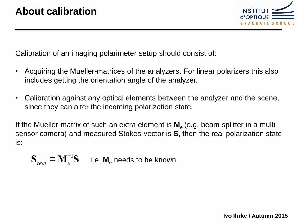
About calibration
Calibration of an imaging polarimeter setup should consist of:
• Acquiring the Mueller-matrices of the analyzers. For linear polarizers this also
includes getting the orientation angle of the analyzer.
• Calibration against any optical elements between the analyzer and the scene,
since they can alter the incoming polarization state.
If the Mueller-matrix of such an extra element is Me (e.g. beam splitter in a multi-
sensor camera) and measured Stokes-vector is S, then the real polarization state
is:
Sreal =Me
-1S i.e. Me needs to be known.
Ivo Ihrke / Autumn 2015
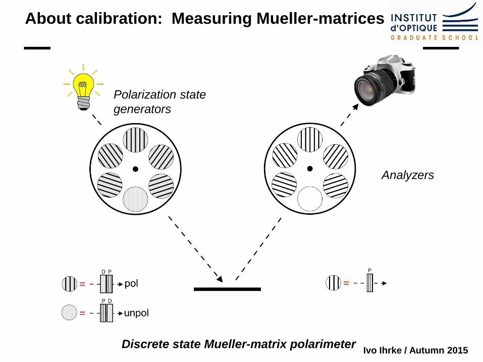
About calibration: Measuring Mueller-matrices
Polarization state
generators
Analyzers
Discrete state Mueller-matrix polarimeter
Ivo Ihrke / Autumn 2015
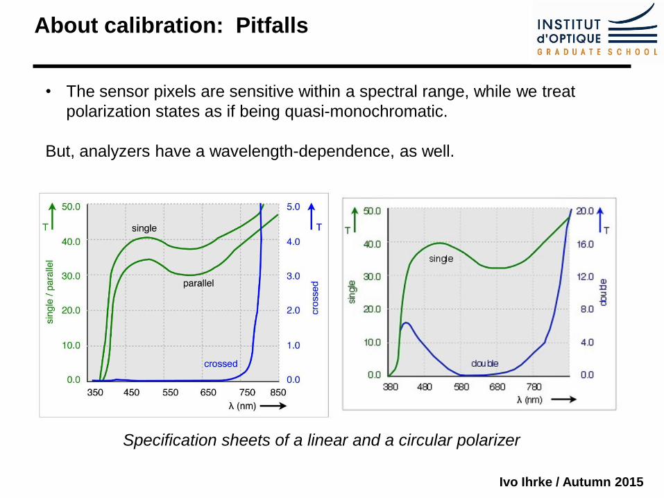
About calibration: Pitfalls
• The sensor pixels are sensitive within a spectral range, while we treat
polarization states as if being quasi-monochromatic.
But, analyzers have a wavelength-dependence, as well.
Specification sheets of a linear and a circular polarizer
Ivo Ihrke / Autumn 2015
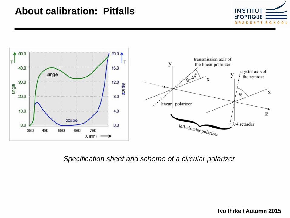
About calibration: Pitfalls
Specification sheet and scheme of a circular polarizer
Ivo Ihrke / Autumn 2015
About calibration: Pitfalls
• Mixing linear polarizers and circular polarizers can be problematic
because of differing spectral absorption properties. Therefore (if circular
polarization is also measured), it is better to use purely circularly
polarizers, as they can act as linear analyzers when flipped.
• Reference polarization states: Generating nearly 100% unpolarized light
is very difficult, usually light sources (except for direct sunlight) are at least
partially polarized.
• Measured Mueller-matrices due to noise can be non-physical
=> need to be checked and rectified when necessary.

Ivo Ihrke / Autumn 2015
Applications
Ivo Ihrke / Autumn 2015
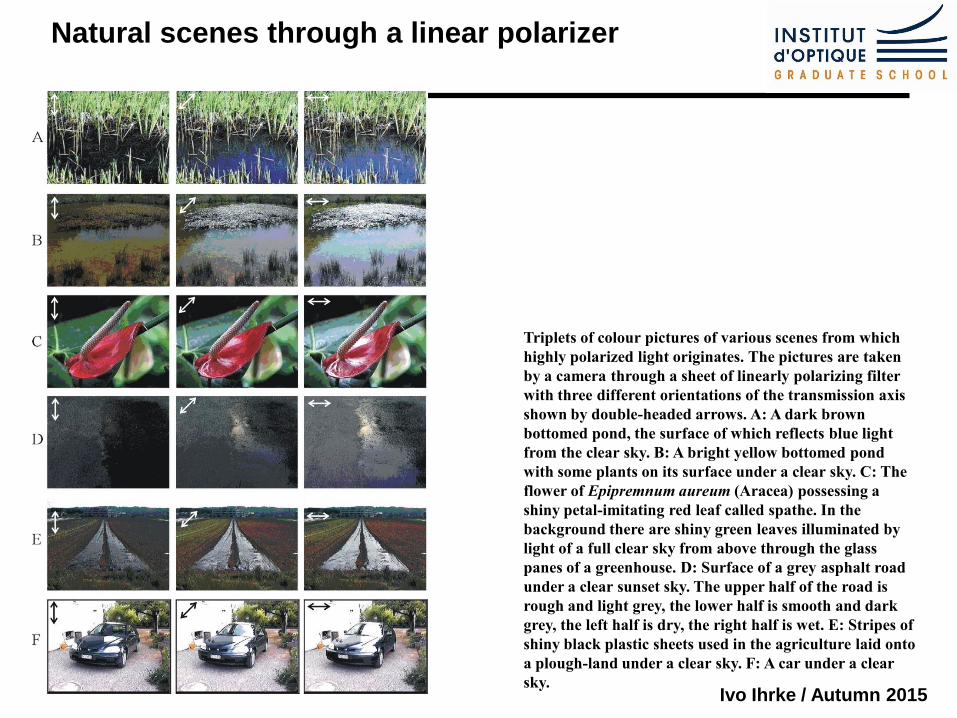
Triplets of colour pictures of various scenes from which
highly polarized light originates. The pictures are taken
by a camera through a sheet of linearly polarizing filter
with three different orientations of the transmission axis
shown by double-headed arrows. A: A dark brown
bottomed pond, the surface of which reflects blue light
from the clear sky. B: A bright yellow bottomed pond
with some plants on its surface under a clear sky. C: The
flower of Epipremnum aureum (Aracea) possessing a
shiny petal-imitating red leaf called spathe. In the
background there are shiny green leaves illuminated by
light of a full clear sky from above through the glass
panes of a greenhouse. D: Surface of a grey asphalt road
under a clear sunset sky. The upper half of the road is
rough and light grey, the lower half is smooth and dark
grey, the left half is dry, the right half is wet. E: Stripes of
shiny black plastic sheets used in the agriculture laid onto
a plough-land under a clear sky. F: A car under a clear
sky.
Our linearly polarized world Natural scenes through a linear polarizer
Ivo Ihrke / Autumn 2015
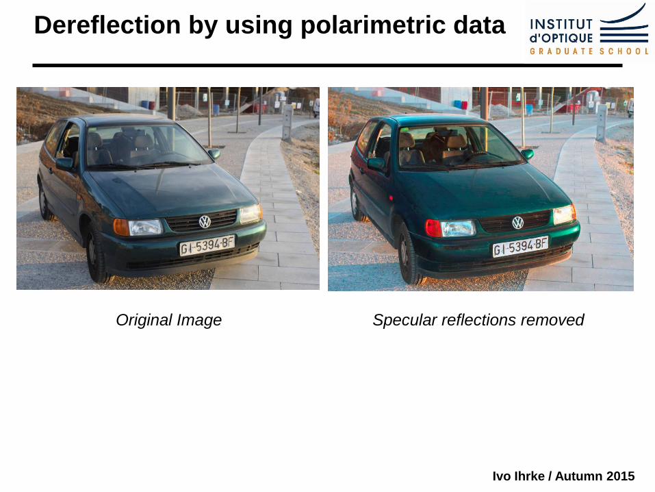
Dereflection by using polarimetric data
Original Image Specular reflections removed
Ivo Ihrke / Autumn 2015
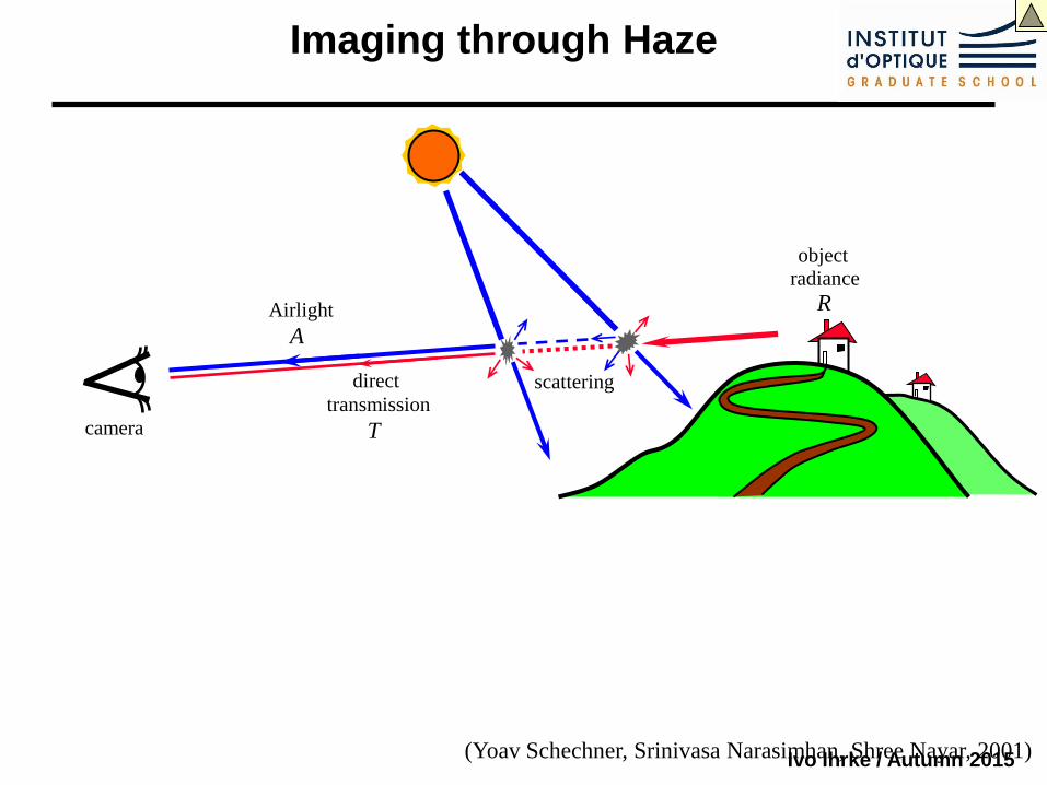
scattering
Airlight
A
direct transmission
T
Imaging through Haze
camera
object radiance
R
(Yoav Schechner, Srinivasa Narasimhan, Shree Nayar, 2001)
Ivo Ihrke / Autumn 2015
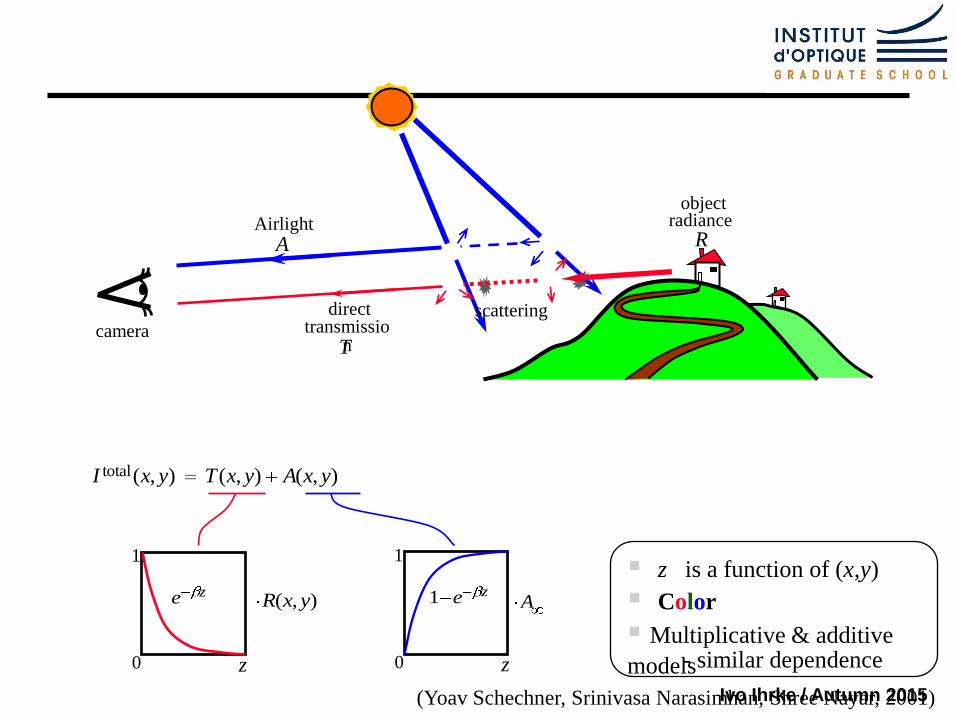
camera
object radiance
R Airlight
A
scattering direct transmissio
n T
0
1
z
ze1 A
0
1
z
ze ),( yxR
),( ),( ),(total yxAyxTyxI
z is a function of (x,y)
Multiplicative & additive
models - similar dependence
Color
(Yoav Schechner, Srinivasa Narasimhan, Shree Nayar, 2001)
Ivo Ihrke / Autumn 2015
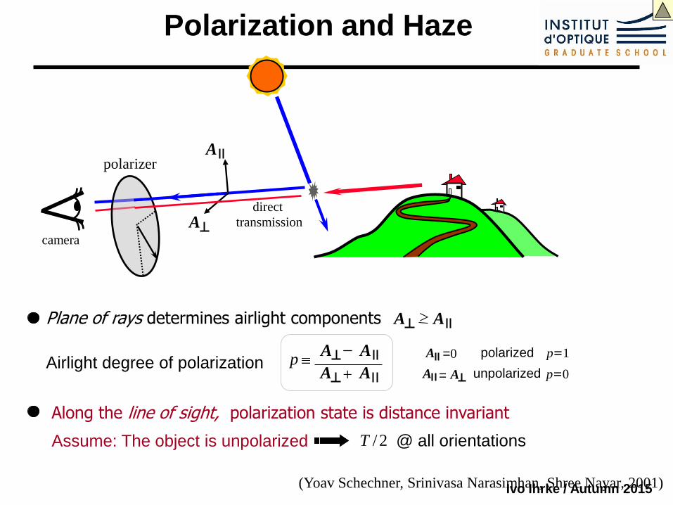
Polarization and Haze
polarizer
camera
A
A
direct transmission
Along the line of sight, polarization state is distance invariant
Assume: The object is unpolarized 2/T @ all orientations
Plane of rays determines airlight components A A >
A A _
A A + pAirlight degree of polarization
p=0 unpolarized A = A
p=1 polarized =0 A
(Yoav Schechner, Srinivasa Narasimhan, Shree Nayar, 2001)
Ivo Ihrke / Autumn 2015
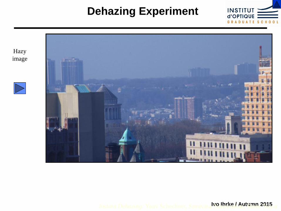
Hazy
image
Dehazing Experiment
Instant Dehazing: Yoav Schechner, Srinivasa Narasimhan, Shree Nayar
Ivo Ihrke / Autumn 2015
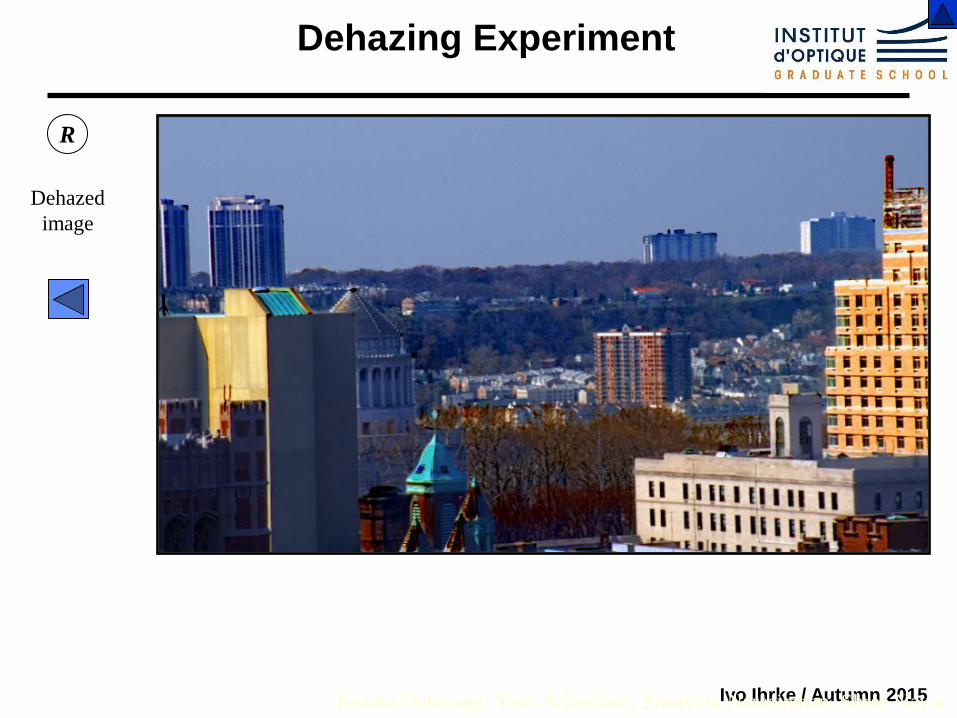
R
Dehazed
image
Instant Dehazing: Yoav Schechner, Srinivasa Narasimhan, Shree Nayar
Dehazing Experiment
Ivo Ihrke / Autumn 2015
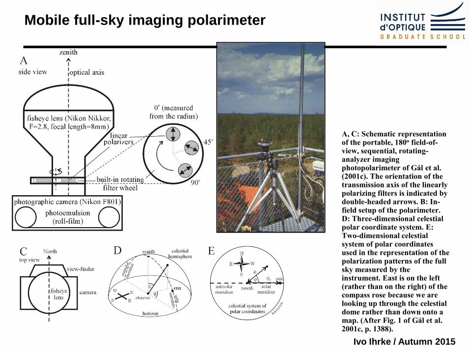
A, C: Schematic representation of the portable, 180o field-of-view, sequential, rotating-analyzer imaging photopolarimeter of Gál et al. (2001c). The orientation of the transmission axis of the linearly polarizing filters is indicated by double-headed arrows. B: In-field setup of the polarimeter. D: Three-dimensional celestial polar coordinate system. E: Two-dimensional celestial system of polar coordinates used in the representation of the polarization patterns of the full sky measured by the instrument. East is on the left (rather than on the right) of the compass rose because we are looking up through the celestial dome rather than down onto a map. (After Fig. 1 of Gál et al. 2001c, p. 1388).
Mobile full-sky imaging polarimeter
Ivo Ihrke / Autumn 2015
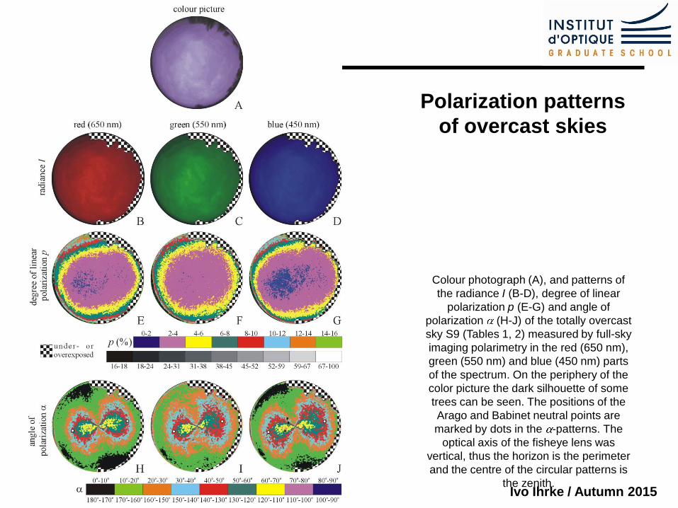
Colour photograph (A), and patterns of
the radiance I (B-D), degree of linear
polarization p (E-G) and angle of
polarization (H-J) of the totally overcast
sky S9 (Tables 1, 2) measured by full-sky
imaging polarimetry in the red (650 nm),
green (550 nm) and blue (450 nm) parts
of the spectrum. On the periphery of the
color picture the dark silhouette of some
trees can be seen. The positions of the
Arago and Babinet neutral points are
marked by dots in the -patterns. The
optical axis of the fisheye lens was
vertical, thus the horizon is the perimeter
and the centre of the circular patterns is
the zenith.
Polarization patterns
of overcast skies
Ivo Ihrke / Autumn 2015
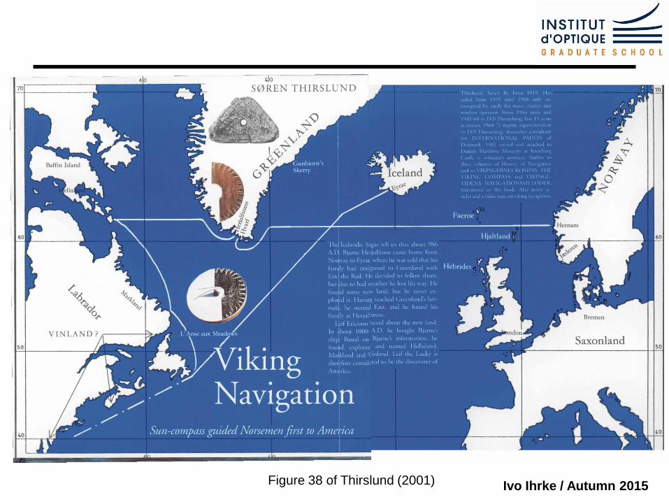
Figure 38 of Thirslund (2001)
Ivo Ihrke / Autumn 2015
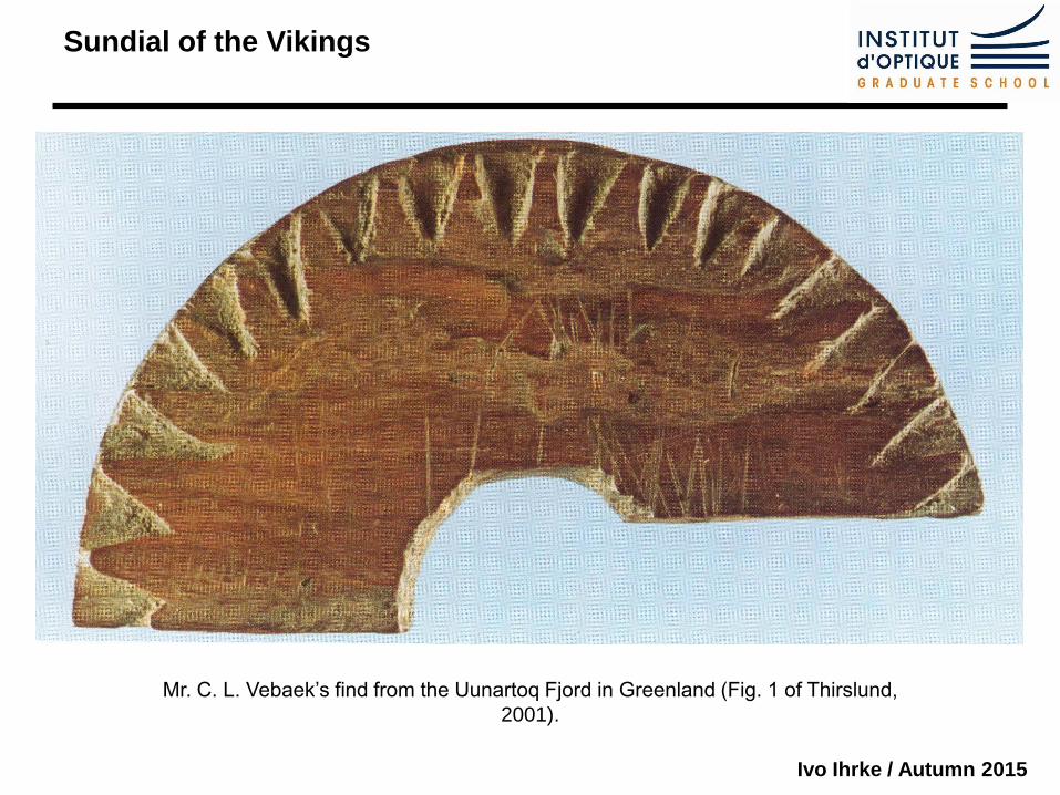
Mr. C. L. Vebaek’s find from the Uunartoq Fjord in Greenland (Fig. 1 of Thirslund,
2001).
Sundial of the Vikings
Ivo Ihrke / Autumn 2015
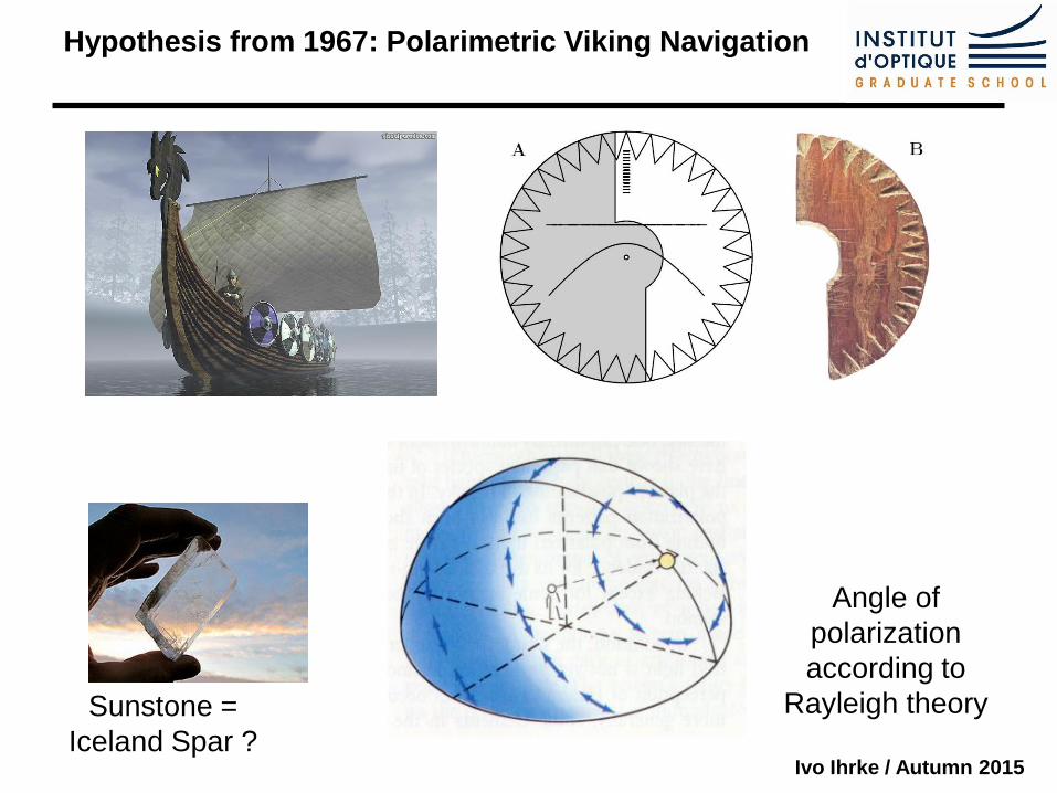
Angle of
polarization
according to
Rayleigh theory
Hypothesis from 1967: Polarimetric Viking Navigation
Sunstone =
Iceland Spar ?
Ivo Ihrke / Autumn 2015
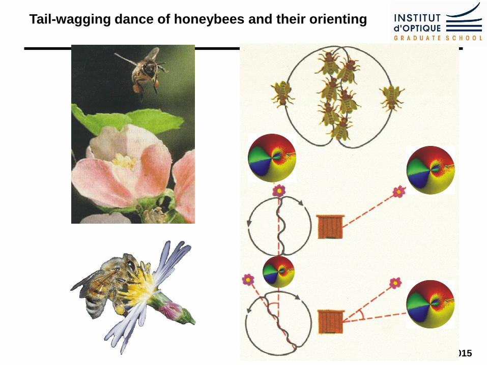
Orientation of honeybees based on skylight polarization Tail-wagging dance of honeybees and their orienting

Ivo Ihrke / Autumn 2015
Next: Deconvolution
Ivo Ihrke / Autumn 2015
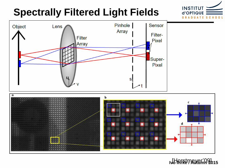
Spectrally Filtered Light Fields
[Horstmeyer’09]
Ivo Ihrke / Autumn 2015
Gabriel Lippmann 1845-1921
t
Ivo Ihrke / Autumn 2015
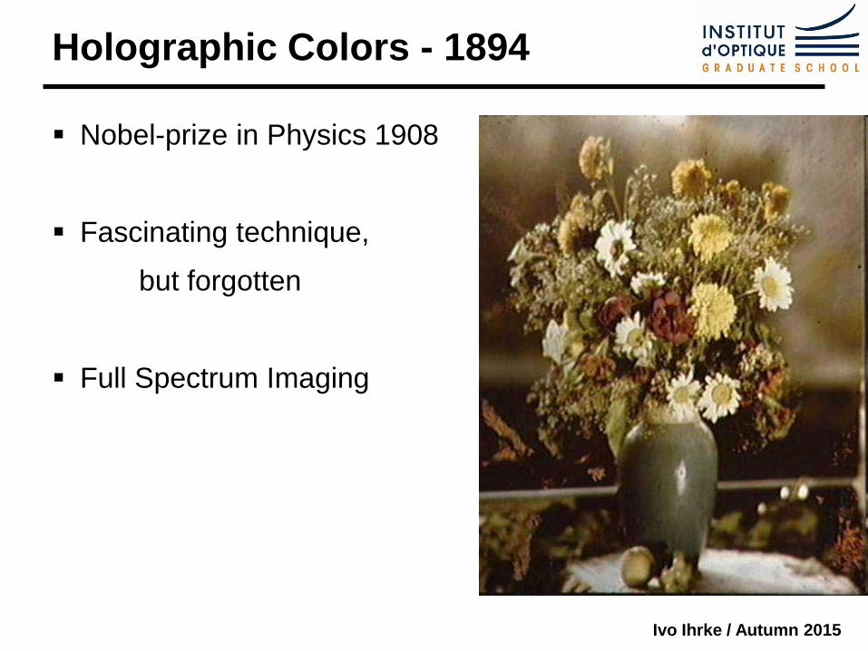
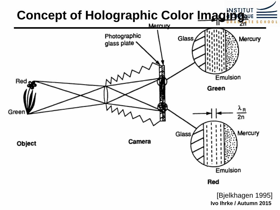
Holographic Colors - 1894
Nobel-prize in Physics 1908
Fascinating technique,
but forgotten
Full Spectrum Imaging
Ivo Ihrke / Autumn 2015
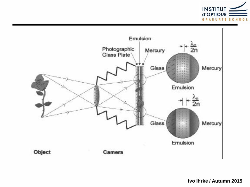
Concept of Holographic Color Imaging
[Bjelkhagen 1995]
Ivo Ihrke / Autumn 2015
Ivo Ihrke / Autumn 2015
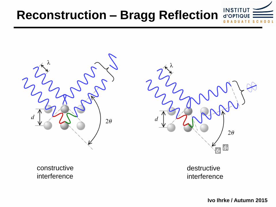
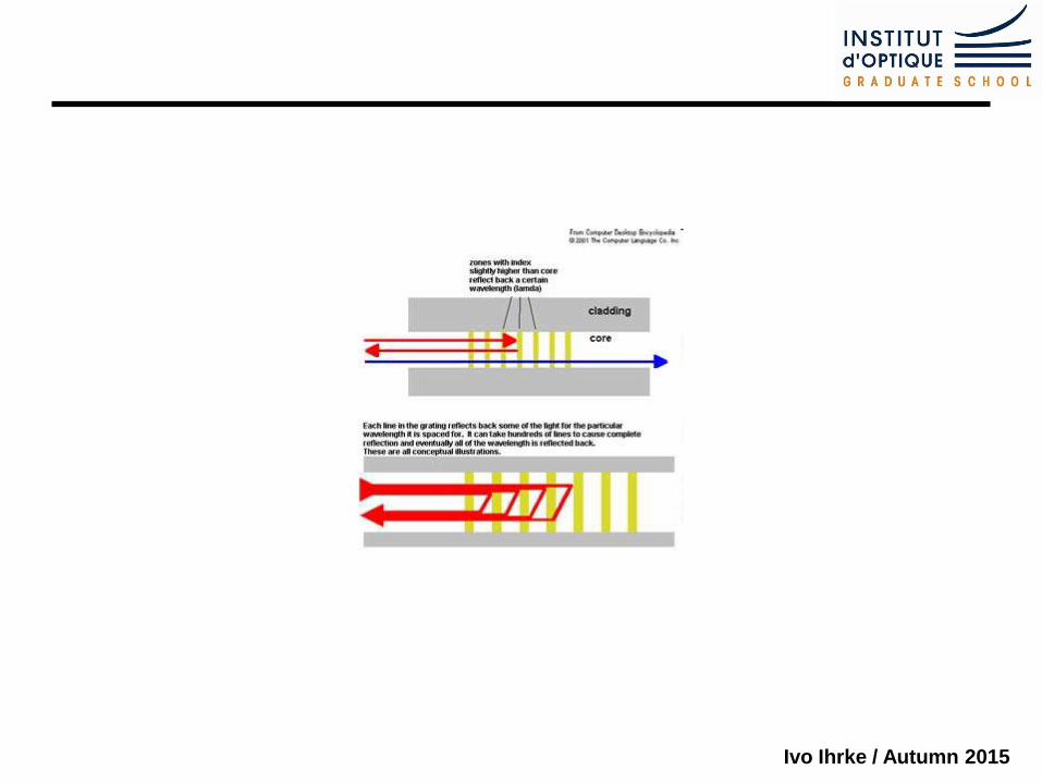
Reconstruction – Bragg Reflection
constructive
interference destructive
interference
Ivo Ihrke / Autumn 2015

Ivo Ihrke / Autumn 2015
Ivo Ihrke / Autumn 2015
Ivo Ihrke / Autumn 2015
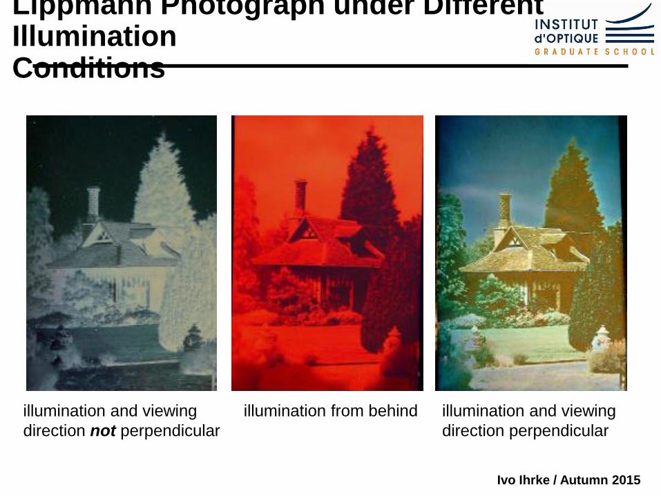
Lippmann Photograph under Different Illumination Conditions
illumination and viewing
direction not perpendicular
illumination and viewing
direction perpendicular
illumination from behind
Ivo Ihrke / Autumn 2015
Bibliography
Holst, G. CCD Arrays, Cameras, and Displays. SPIE Optical
Engineering Press, Bellingham, Washington, 1998.
Theuwissen, A. Solid-State Imaging with Charge- Coupled Devices. Kluwer Academic Publishers, Boston, 1995.
Curless, CSE558 lecture notes (UW, Spring 01).
El Gamal et al., EE392b lecture notes (Spring 01).
Several Kodak Application Notes at http://www.kodak.com/global/en/digital/ccd/publications/applicationNotes.jhtml
Reibel et al., CCD or CMOS camera noise characterization, Eur. Phys. J. AP 21, 2003
Ivo Ihrke / Autumn 2015
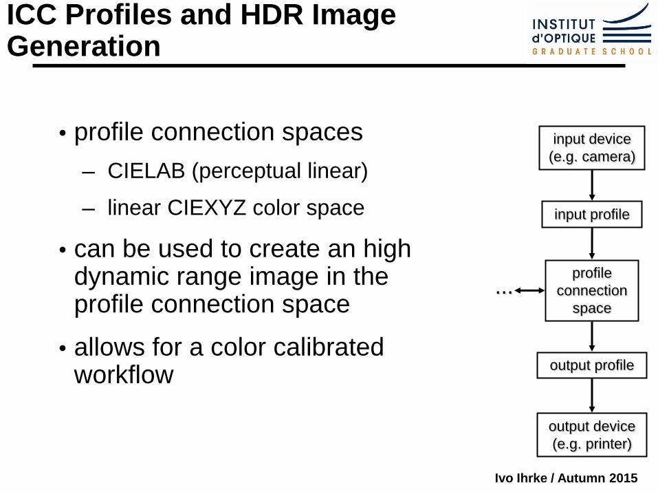
profile connection spaces
─ CIELAB (perceptual linear)
─ linear CIEXYZ color space
can be used to create an high dynamic range image in the profile connection space
allows for a color calibrated workflow
ICC Profiles and HDR Image Generation
input device
(e.g. camera)
input profile
profile
connection
space
output device
(e.g. printer)
output profile
...