computational synthetic biology -...
TRANSCRIPT

ComputationalComputational
Synthetic BiologySynthetic Biology
Yiannis N. Kaznessis
University of MinnesotaDepartment of Chemical Engineering and Materials Science
OutlineOutlineOutlineOutline
Synthetic biology.Synthetic biology. What is it?
How can computational modeling assist synthetic biology?
Stochasticity and the need for multiscale models
Synthetic Biology Software SuiteHybrid stochastic algorithms. Desktop simulation engines.
SynBioSS Designer. BioBricks and synthetic biology standards.
S Bi SS WikiSynBioSS Wiki
Example: Computer‐aided design of bio‐logical AND gates.

Synthetic BiologySynthetic BiologySynthetic BiologySynthetic BiologyWith Genome Projects toolboxes become available of
Regulatory proteins (activators and repressors)Operator and promoter sitesS ll i d l lSmall inducer molecules
DNA can be cut and pasted!p
Novel gene regulatory networks are at hand.
Synthetic biology: Emphasis on systems (not your grandfather’s genetic engineering).g g g)

Example Example of of Synthetic BiologySynthetic BiologyBistable switch, Gardner and Collins (2000)
DNA plasmid sequences Network topology
Dynamicbehavior
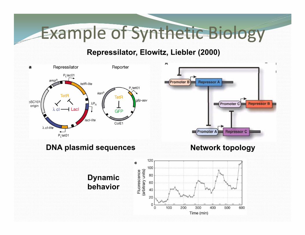
Example Example of of Synthetic BiologySynthetic BiologyRepressilator, Elowitz, Liebler (2000)
DNA plasmid sequences Network topology
Dynamicbehavior

Synthetic BiologySynthetic BiologyPrecise control of the response of biological systems.
Switches (e g if Ci d >0 then turn on production of protein A)Switches (e.g. if Cinducer>0 then turn on production of protein A)
Amplitude filters (e.g. if Cinducer>Cthreshold then turn on production of protein A)protein A)
Logical operators (e.g. if signal molecule 1 AND signal molecule 2 are present then turn on production of protein A)present, then turn on production of protein A)
Numerous applications (e.g. gene therapy, sensors, biosynthetic d ti ti i ti bi l i l ti )production optimization, biological computing)

Synthetic Biology ChallengeSynthetic Biology Challenge
DNAsequencesq
ATGGCATATGGTTATGGCATATGGTTATGGCATATGGTTATGGCATATGGTT
Phenotypic dynamicbehavior
Given a targeted dynamic phenotype, how do we engineer a gene regulatorynetwork and choose a particular DNA sequence? If we want to engineer annetwork and choose a particular DNA sequence? If we want to engineer anoscillator, what genes do we use and how do we connect them? Or, if we have acertain gene regulatory network can we predict its dynamic phenotype?

Modeling Gene NetworksModeling Gene NetworksggProtein Dimer Inducer BindingModeling rationalizes forward
engineering
mRNARNAp
g g
Modeling all interactions at the mRNA
genepromoter
molecular level• Protein Interactions• Transcription
mRNA ribosome
Protein product• Transcription• Translation• Regulation
RNAp repressorRNApactivator
Regulation
geneoperatorgenepromoteroperator promoter

Chemical Kinetic ModelsChemical Kinetic ModelsCascades of reactions represent biomolecular interactions
1
2
+ ⎯⎯→
⎯⎯→ +
k
k
A B C
C A BAA BB
Two levels of design degrees of freedom:1. Network topology (e.g. TetR represses LacI, LacI
represses Ara, Ara represses TetR)2 Kinetic constant (e g TetR binds tetO1 TetR binds2. Kinetic constant (e.g. TetR binds tetO1, TetR binds
tetO2)

ExampleExample (Sotiropoulos and Kaznessis BMC Systems Biology (2007))

Gene network modelingGene network modelingGe e et o ode gGe e et o ode gDescribe/predict the dynamic behavior quantitatively.
Model networks of biomolecular interactions (dozens to hundreds ofModel networks of biomolecular interactions (dozens to hundreds of species)
1k
RNAp
Deterministic kinetics
1
1
RNAp + P RNAp:Pk −
↔promoterDeterministic kinetics
1 -1d[RNAp:P] = k [RNAp] [P] - k [RNAp:P]
dt
A set of ordinary differential equations would result. This modeling formalism is not accurate.
dt
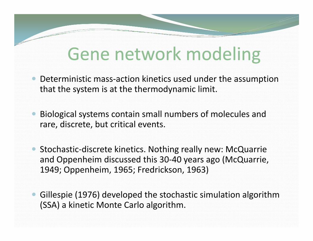
Gene network modelingGene network modelingDeterministic mass‐action kinetics used under the assumption that the system is at the thermodynamic limit.
Biological systems contain small numbers of molecules and rare, discrete, but critical events.
Stochastic‐discrete kinetics. Nothing really new: McQuarrieand Oppenheim discussed this 30‐40 years ago (McQuarrie,
h k )1949; Oppenheim, 1965; Fredrickson, 1963)
Gillespie (1976) developed the stochastic simulation algorithmGillespie (1976) developed the stochastic simulation algorithm (SSA) a kinetic Monte Carlo algorithm.

Stochastic Simulation AlgorithmStochastic Simulation Algorithm• N species react through M reaction channels.
• X (t) is the number of molecules of speciesModel
• Xi(t) is the number of molecules of species i, in the system at time t.
Algorithm
• Determine probability that, starting at time t, reaction μ, Rμ, will be the next reaction to occur in the interval [t+τ, t +τ+dτ]
• Execute reaction μ and propagate timeAlgorithm • Execute reaction μ and propagate time.
• The system may contain rare, discrete, but critical events andcontinuously occurring deterministic or stochastic transitions.
• Simulation using the SSA will be very slow. Computational time scales with the number of reaction occurrences .

MultiscaleMultiscale Modeling FrameworkModeling FrameworkggI: Discrete / Stochastic
Jump Markov processStochastic simulation algorithm
Reaction rate (propensity)Stochastic simulation algorithm (Gibson and Bruck, 2000)
II: Discrete / StochasticTau‐Leaping (Cao Petzold
λ
I II Tau‐Leaping (Cao, Petzold, Gillespie, 2005)Probabilistic steady state
III‐IV: Continuous / Stochasticε
I
olec
ules
II
III‐IV: Continuous / StochasticValid continuous Markov process Chemical Langevin equation(Gillespie 2001; Haseltine andm
ber o
f mo
III IV(Gillespie, 2001; Haseltine and Rawlings, 2002)
V: Continuous / DeterministicValid ordinary differential
Num
VValid ordinary differential equations (Amundson, 1966)
Petzold, Gillespie, Cao, Vlachos, Kevrekidis, Vanden-Eijnden, Arkin, Khammash

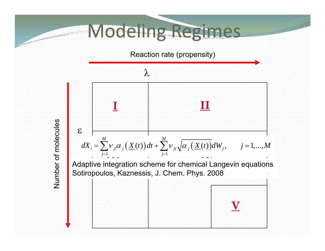
Modeling Modeling RegimesRegimes
λ
Reaction rate (propensity)
I II( )1l n0 1
aτ Σ
⎛ ⎞⎟⎜ ⎟← ⎜ ⎟⎜ ⎟⎟⎜⎝ ⎠U
ε
lecu
les
( )0 , 1 ⎟⎜⎝ ⎠U
Integrate stochastic-discrete and stochastic-continuous modelsHy3S Salis and Kaznessis J Chem Phys 2005
ber o
f mol
III IV( ) ( )1 1
( ) ( ) , 1,...,M M
i ji j ji j jj j
dX X t dt X t dW j Mν α ν α= =
= + =∑ ∑
Hy3S, Salis and Kaznessis, J.Chem. Phys. 2005
Num
V
1 1j j= =
V

Hybrid EquationsHybrid EquationsPa tition into slo /dis ete and fast/ ontin o s ea tions (HaseltinePartition into slow/discrete and fast/continuous reactions (Haseltine, Rawlings, 2002)
The effects of the fast/continuous reactions are described by ItôSDEs, called the chemical Langevin equation
fast fastM M
( ) ( )M M
f fi ji j ji j j
j=1 j=1dX = v a X(t) dt+ v a X(t) dW∑ ∑
The times of the slow/discrete reaction events are governed by a system of differential Jump equations, describing the time evolution of the reaction residuals, Rjj
When Rj(t) = 0, then the jth reaction has occurred at time t.
These are also Itô SDEs, but without a Wiener process, W
s slowj j j o jdR = a (X(t))dt, R (t ) = log(URN ), j =1...M

SDE integrationSDE integrationEuler-Maruyama Scheme, numerical error α √(∆t)
fast fastM M
SDE integrationSDE integration
fast fastM Mf f
i i ji j ji j jj=1 j=1
X (t+Dt)=X (t)+ v a (X(t))Dt+ v a (X(t))DW∑ ∑
( ) ( ( ))sR R X∆ ∆Milstein Scheme, numerical error O(∆t)
( ) ( ( )) sj jR t t R a X t t+ ∆ = + ∆
1 1
( ) ( ) ( ( )) ( ( ))fast fastM M
f fi i ji j ji j j
j j
X t t X t v a X t t v a X t W= =
+ ∆ = + ∆ + ∆∑ ∑
1 1
1 2
1 2 2
1 2, 1 1
( ( ))1 ( , )2 ( ( ))
fast
j j
M Nj j
j n j ij j n j n
a X t av v I j j
a X t X= =
∂+
∂∑ ∑1 2 2, ( ( ))j j n j n

Speed Comparisons with SSASpeed Comparisons with SSAThe Cycle Test
System Size proportional to the1kA B⎯⎯→System Size proportional to the
number of reactant molecules of fast reactions
2k
k
B CC⎯⎯→
Ratios of Computational Run TimesSystem
3
4
k
k
C DA C D⎯⎯→
+ ⎯⎯→System Size TSSA/TNRH TSSA/TANRH
1001000
7.9495 59
9.64116 1
5kB C E+ ⎯⎯→1000
10,000100,000
95.59986.816912
116.11198.220535
1 2 3 4 5, , ,k k k k k<<
Large scale benchmark in Salis and Kaznessis J.Chem.Phys. 2005a
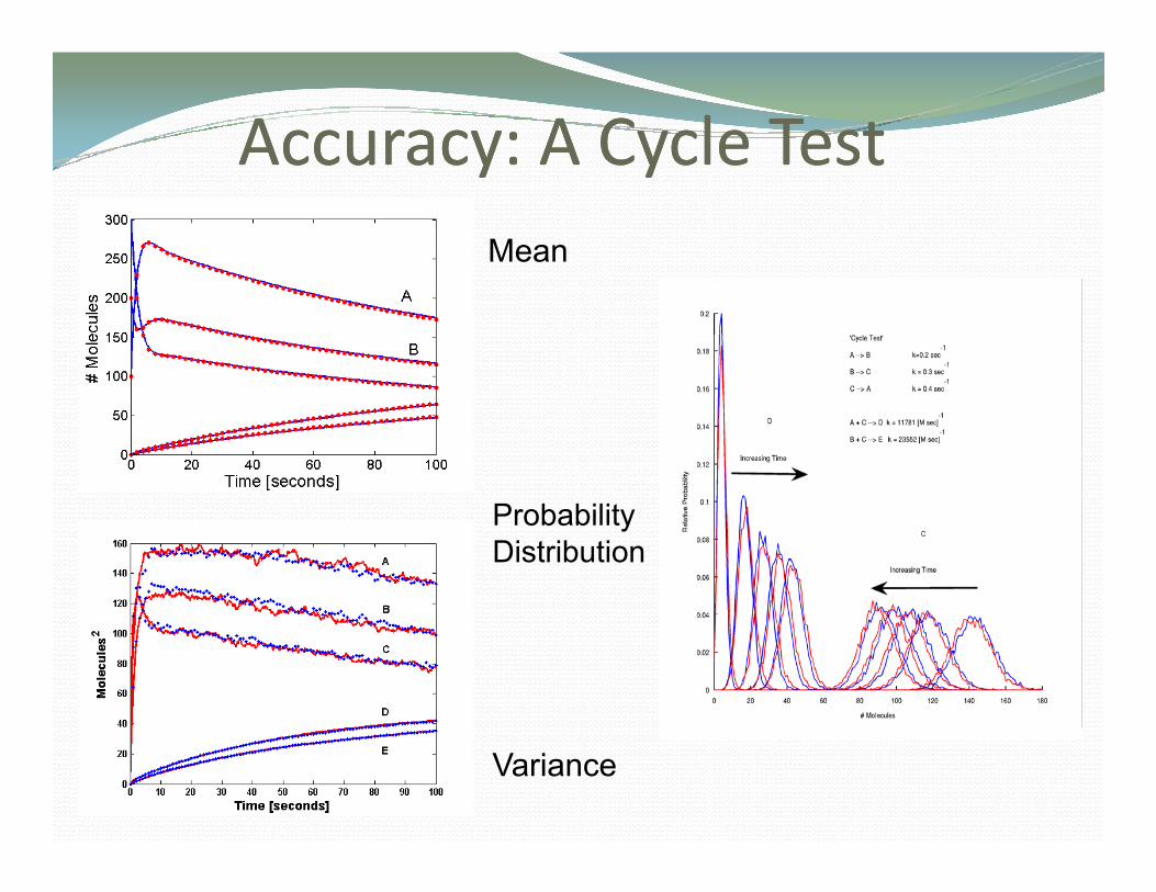
Accuracy: A Cycle TestAccuracy: A Cycle Testccu acy Cyc e estccu acy Cyc e estMean
Probability Distribution
Variance

Modeling Modeling RegimesRegimes
λ
Reaction rate (propensity)
I II( )1ln0 , 1
aτ Σ
⎛ ⎞⎟⎜ ⎟← ⎜ ⎟⎜ ⎟⎟⎜⎝ ⎠U
1 1 1 1( , ; | ( ), ) ( ; | ) ( ; | ( ), )
1( ) ( ) ( ) '
f s s f f
t TSS
P X X t X t t P X t X P X t X t t
f X P X dX f t dt+
=
=∫ ∫
ε
lecu
les
( ),⎝ ⎠ ( ) ( ) ( )t
f X P X dX f t dtTΩ
=∫ ∫
Probabilistic steady state approximationSalis and Kaznessis J Chem Phys 2005b
ber o
f mol
III IV
Salis and Kaznessis, J.Chem. Phys. 2005b
Num
VV
Modeling Modeling RegimesRegimes
λ
Reaction rate (propensity)
I II
ε
lecu
les
M M
∑ ∑
ber o
f mol
III IV( ) ( )
1 1( ) ( ) , 1,...,i ji j ji j j
j jdX X t dt X t dW j Mν α ν α
= =
= + =∑ ∑Adaptive integration scheme for chemical Langevin equationsSotiropoulos Kaznessis J Chem Phys 2008
Num
V
Sotiropoulos, Kaznessis, J. Chem. Phys. 2008
V
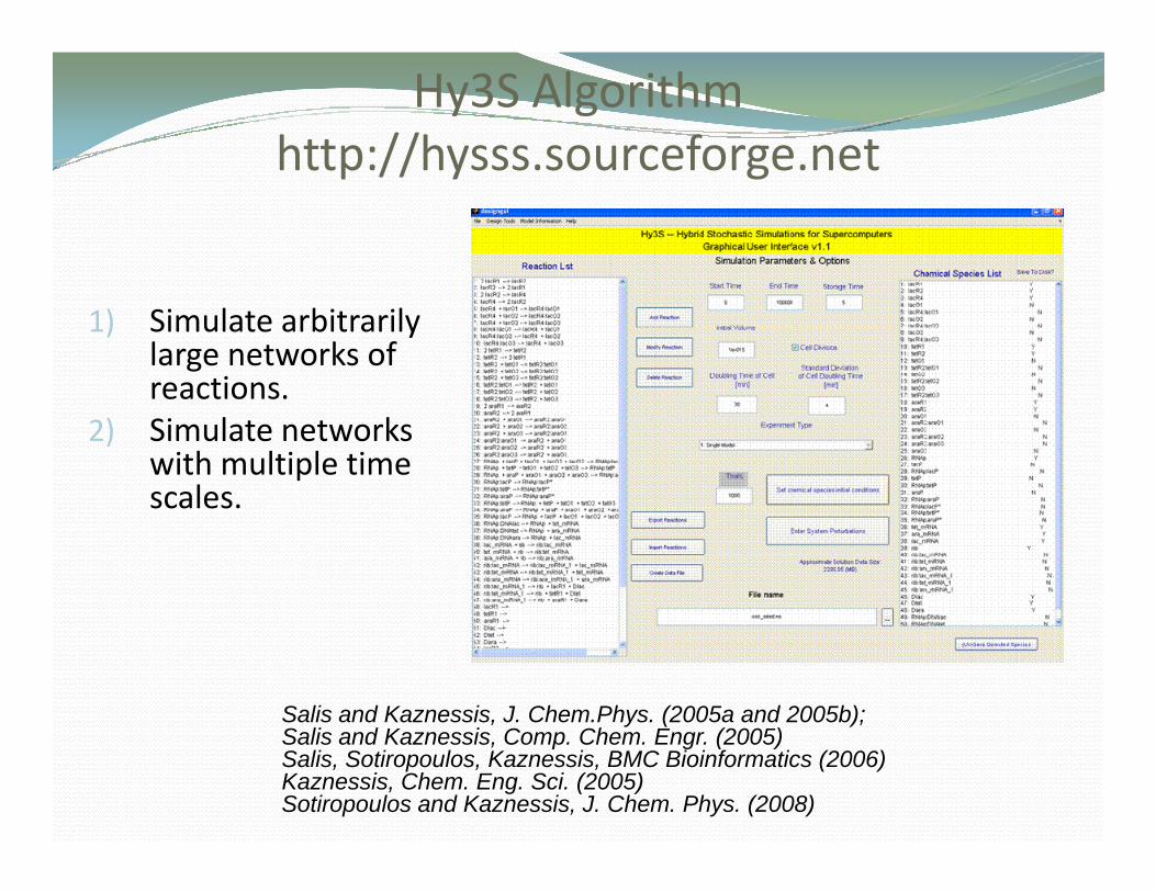
Hy3S Algorithm http://hysss.sourceforge.nethttp://hysss.sourceforge.net
1) Simulate arbitrarily large networks of reactionsreactions.
2) Simulate networks with multiple time scalesscales.
Salis and Kaznessis, J. Chem.Phys. (2005a and 2005b); S C C ( )Salis and Kaznessis, Comp. Chem. Engr. (2005)Salis, Sotiropoulos, Kaznessis, BMC Bioinformatics (2006)Kaznessis, Chem. Eng. Sci. (2005)Sotiropoulos and Kaznessis, J. Chem. Phys. (2008)
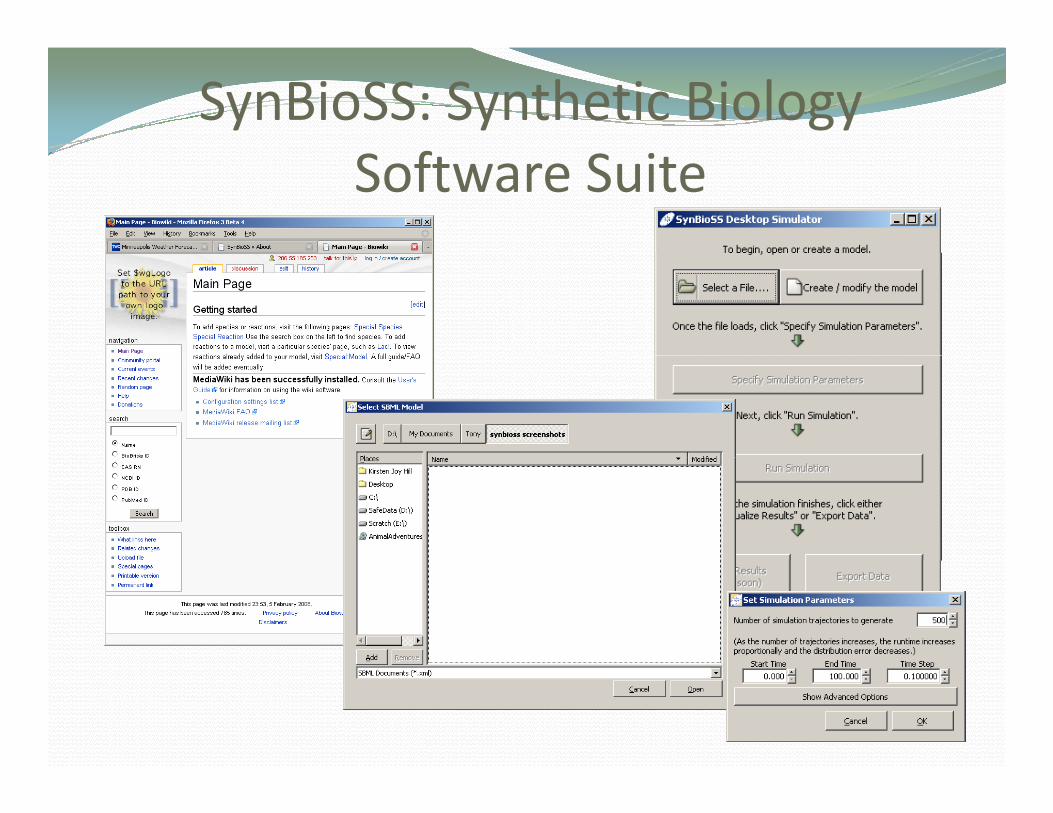
SynBioSS: Synthetic Biology Software Suite
SynBioSSThe Synthetic Biology Software Suite is a software suite for the generation,
storing, retrieval and quantitative simulation of synthetic biological networks.SynBioSS facilitates computational synthetic biology and consists of three
independent components: the Desktop Simulator (DS) the Wiki and theindependent components: the Desktop Simulator (DS), the Wiki, and the Designer.
The SynBioSS DS is a set of multiscale algorithms for modeling and simulating reaction networks, such as gene regulatory networks. It combines routines for modeling systems stochastically and discretely (kinetic Monte Carlo) and/or stochastically and continuously (stochastic differential equations).
SynBioSS has a user friendly graphical user interface, and it reads and writes SBML and nc modelsSBML and .nc models.
SynBioSS DS can run on Windows, Mac OS, and Linux/UNIX. It is an Open Source software and can be downloaded at SourceForge.
SynBioSS Designer is a web service to transform a sequence of BioBricks, or any other set of biomolecular components, to a set of reactions that can be simulated dynamically in SynBioSS DS.
SynBioSS Wiki is a web service to collect the kinetic parameters necessary to create a model that can be simulated by SynBioSS DS.create a model that can be simulated by SynBioSS DS.

http://synbioss.sourceforge.net/http://synbioss.sourceforge.net/Partitioned stochastic simulation:
Currently built around Hy3S y y(Hybrid Jump-Continous Markov Stochastic Simulator)Extendible to any integrator (StochKit etc )(StochKit, etc.)
GUI is built in cross-platform Python & GTKImports SBMLImports SBML
Converts to Hy3S native NetCDF input files for simulation
User can edit / create a model from within the GUIBuilt to have intelligent defaults, to be minimally confusingto be minimally confusing.

The algorithms used were developed by the Kaznessis research group at theUniversity of Minnesota, Dept. of Chemical Engineering and Materials Science.This work is supported by a CAREER award to YNK (NSF 0644792) NotableThis work is supported by a CAREER award to YNK (NSF 0644792). Notablecontributions have been made by: Howard Salis, Vassilios Sotiropoulos, AnthonyD. Hill, and Jonathan R. Tomshine.SynBioSS is licensed under the GPL, and may be redistributed under the sametermsterms.

http://synbioss.sourceforge.net/http://synbioss.sourceforge.net/Download SynBioSS installer from sourceforge.net
All the examples are based on the Windows version. Available Linux/UNIX versions should work in a similar manner (the Linux/UNIX distribution of SynBioSS will require manually linking Python libraries and the installation procedure will vary depending on the specific architecture We have triedprocedure will vary depending on the specific architecture. We have tried IBM, Sun, SGI architectures succeffully). There is currently a beta version of SynBioSS for MacOS being tested.
Run the installerRun the installer.
It will install SynBioSS in C:\Program Files\SynBioSSunless told otherwise.
Click on Start menu and find SynBioSS. Create desktop short cut if so desired.
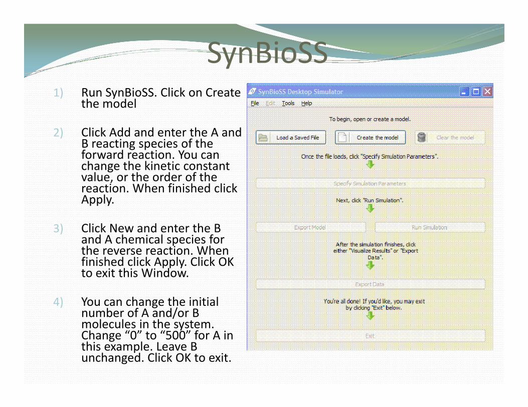
SynBioSS1) Run SynBioSS. Click on Create
the model
2) Click Add and enter the A and B reacting species of the forward reaction. You can change the kinetic constant value or the order of thevalue, or the order of the reaction. When finished click Apply.
3) Click New and enter the B3) Click New and enter the B and A chemical species for the reverse reaction. When finished click Apply. Click OK to exit this Window.
4) You can change the initial number of A and/or B molecules in the system. Ch “0” t “500” f A iChange “0” to “500” for A in this example. Leave B unchanged. Click OK to exit.
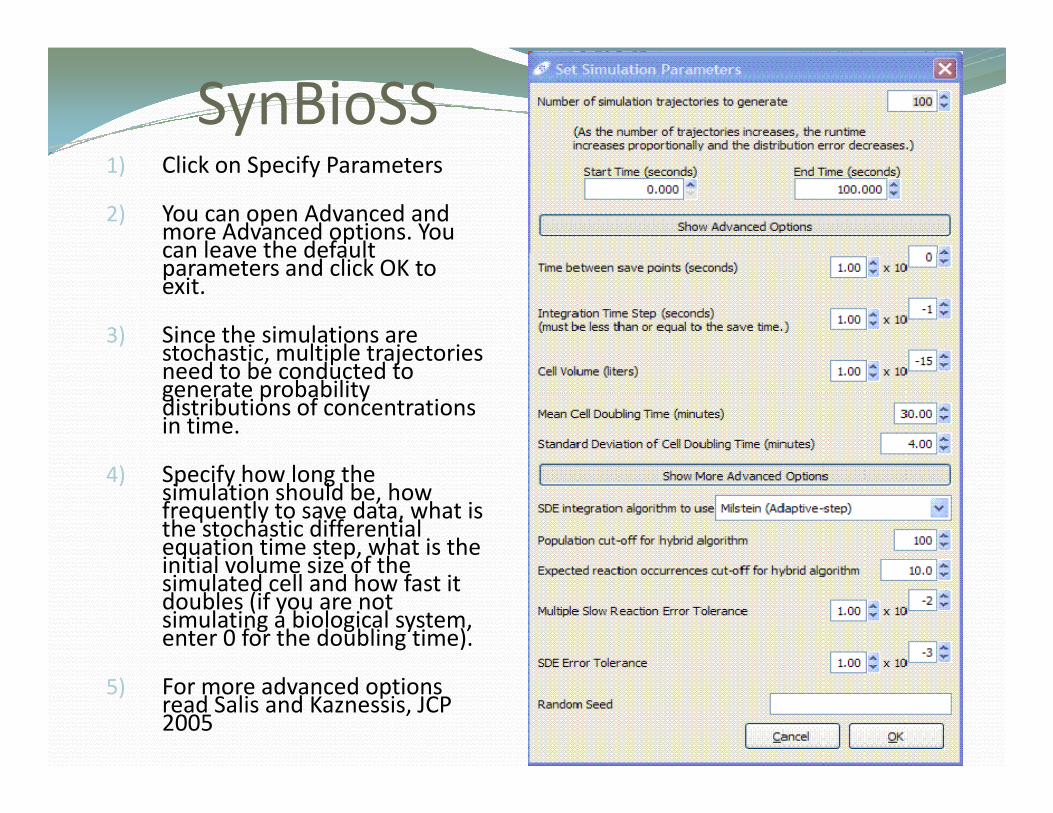
SynBioSS1) Click on Specify Parameters
2) You can open Advanced and more Advanced options. You can leave the defaultcan leave the default parameters and click OK to exit.
3) Since the simulations are stochastic multiple trajectoriesstochastic, multiple trajectories need to be conducted to generate probability distributions of concentrations in time.
4) Specify how long the simulation should be, how frequently to save data, what is the stochastic differential equation time step, what is the i iti l l i f thinitial volume size of the simulated cell and how fast it doubles (if you are not simulating a biological system, enter 0 for the doubling time).
5) For more advanced options read Salis and Kaznessis, JCP 2005

SynBioSS1) Run the simulation. A new
window will appear with information on the progress of the simulation.progress of the simulation.
2) You can export the model at any time. You can cansave it as a SBML file or a
fil h l i.nc file. The latter is a NetCDF file and is a more appropriate file format for very large systems, and long simulations inlong simulations in supercomputers, because a user can search and extract information very quickly.
3) Click on Export Data. You can write the data (concentration profiles as a function of time for each one of the stochastic trajectories) in csv format read by Excel.

More AnalysisCalculate the Average amount of “A” at each time point
Set CX2 to ‘=average(B2:CW2)’
Click and drag to fill to all time‐points
Calculate the Standard Deviation of “A” at each time point:point:
Set CY2 to ‘=stdev(B2:CW2)’
Click and drag to fill to all time‐pointsClick and drag to fill to all time points

A↔B
SynBioSS Designery gGenerating models for gene regulatory networks is challenging:
1) how exactly to model transcription, translation, regulation, induction, etc.? ,
2) Where to find kinetic parameters?
SynBioSS Designer resolves the first challenge. SynBioSS Wiki assists ith th dwith the second.
The SynBioSS Designer uses a network of biomolecular components to generate a list of molecular‐level reactions which describe the greaction network network. This list is exported as a NetCDF file which may be opened by the SynBioSS Simulator or Hy3s.
SynBioSS Designer was built to accept any arbitrary molecularSynBioSS Designer was built to accept any arbitrary molecular component (promoter, transcription factor, inducer molecule, etc.)
l d d k h d d f hIt is also designed to accept BioBricks, the standard of synthetic molecular biology parts (http://parts.mit.edu).

http://www.partsregistry.org/Main_Page
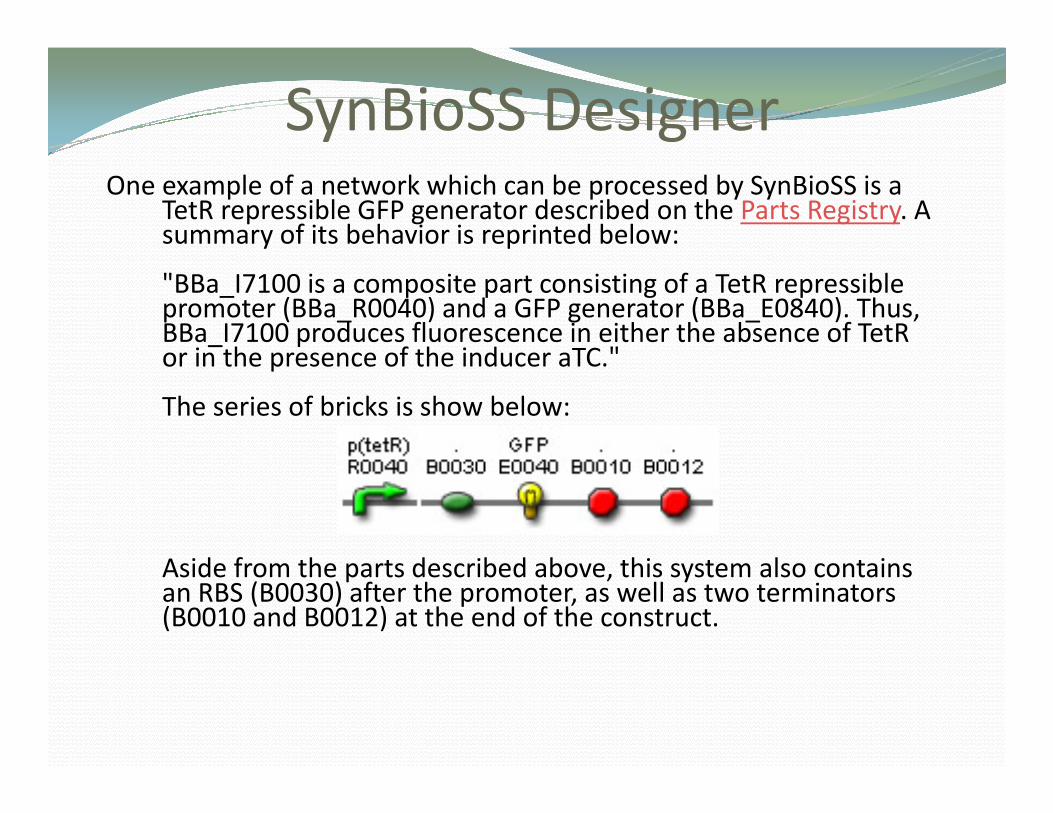
SynBioSS DesignerOne example of a network which can be processed by SynBioSS is a
TetR repressible GFP generator described on the Parts Registry. A summary of its behavior is reprinted below:
"BBa_I7100 is a composite part consisting of a TetR repressible promoter (BBa_R0040) and a GFP generator (BBa_E0840). Thus, BBa_I7100 produces fluorescence in either the absence of TetRor in the presence of the inducer aTC "or in the presence of the inducer aTC.
The series of bricks is show below:
A id f th t d ib d b thi t l t iAside from the parts described above, this system also contains an RBS (B0030) after the promoter, as well as two terminators (B0010 and B0012) at the end of the construct.

SynBioSS DesignerThe first step is to input the BioBricks for the network. It is
important to enter the parts in order, from left to right. To input a brick in the web interface simply type in the brick'sinput a brick in the web interface, simply type in the brick s ID and select its "type" (e.g. promoter). The GFP generator is input as follows (clicking the 'Add Biobrick' button for each brick):)
The "Current BioBricks" table should now look like this:

SynBioSS DesignerA i di d h h i d ddi i l i f iAs indicated here, the Designer needs additional information on
coding DNA and promoters. For coding DNA, the user must input the protein which is produced; in this case, it is GFP. To input this information, select the coding DNA's ID (E0040) from the drop‐down menu in the "Coding DNA Specifics" section, enter thedown menu in the Coding DNA Specifics section, enter the protein's name (GFP), and click "Add Protein".
For promoters, the user must input the operator sites on the promoter. This information can be found at the promoter's page on the Parts Registry. This promoter contains two operator sites. To input them, select the promoter's ID (R0040) from the drop‐down menu in the "Promoter Specifics" section enter thedown menu in the "Promoter Specifics" section, enter the operator's name, and click "Add Operator". The order of the operators does not matter, nor do their names. We shall call them tetO1 and tetO2:
The "Current BioBricks" table is now complete:The Current BioBricks table is now complete:
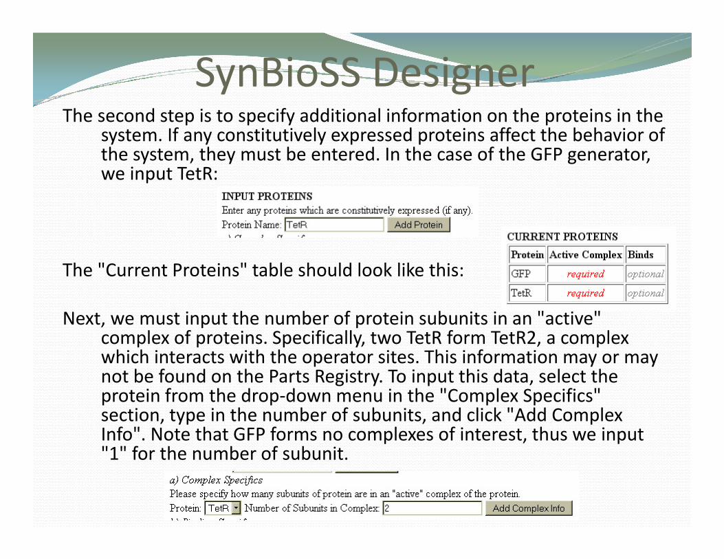
SynBioSS DesignerThe second step is to specify additional information on the proteins in the
system. If any constitutively expressed proteins affect the behavior of the system, they must be entered. In the case of the GFP generator, we input TetR:we input TetR:
The "Current Proteins" table should look like this:
N t t i t th b f t i b it i " ti "Next, we must input the number of protein subunits in an "active" complex of proteins. Specifically, two TetR form TetR2, a complex which interacts with the operator sites. This information may or may not be found on the Parts Registry. To input this data, select the g y pprotein from the drop‐down menu in the "Complex Specifics" section, type in the number of subunits, and click "Add Complex Info". Note that GFP forms no complexes of interest, thus we input "1" for the number of subunit1 for the number of subunit.

SynBioSS DesignerFinally, we must indicate the operator sites to which proteins may
bind. To do so, select the protein and one operator which it binds from the drop‐down menus in the "Binding Specifics" section, and click "Add Binding Info". The order in which yousection, and click Add Binding Info . The order in which you enter the operators does not matter, and not all proteins need to bind to something:
The "Current Proteins" table is now complete:

SynBioSS DesignerThe final step is to specify information on the inducer molecules in the system (if
any). Recall that the inducer "aTc" is an important species in the GFP generator system. Add it:
Finally, we must specify how many times each inducer can bind to a protein complex. In our example system, aTc can bind to TetR2 a maximum of two times. To enter this information, select the inducer and protein from the drop‐down menus in the "Inducer Specifics" section, enter the maximum number of times the inducer can bind to the complex (NOT the individualnumber of times the inducer can bind to the complex (NOT the individual protein, unless it does not form a complex), and click "Add Inducer Info". For our system:
The "Current Inducer" table is now finishedThe "Current Inducer" table is now finished

SynBioSS DesignerThe Designer now has enough information to generate a detailed, molecular‐level model for this system of BioBricks. Click "Generate .nc File"
h d l hi h h b d i h S Bi SS Si lto save the model, which can then be opened in the SynBioSS Simulator or Hy3s.
Automated generation of kinetic modelsFrom DNA level‐‐‐ATGCGCTATAGCTTATGC‐‐‐
User input via web interface
BioBricksSpecifics:p
Operators
Proteins
Effectors
NetCDF, SBML output
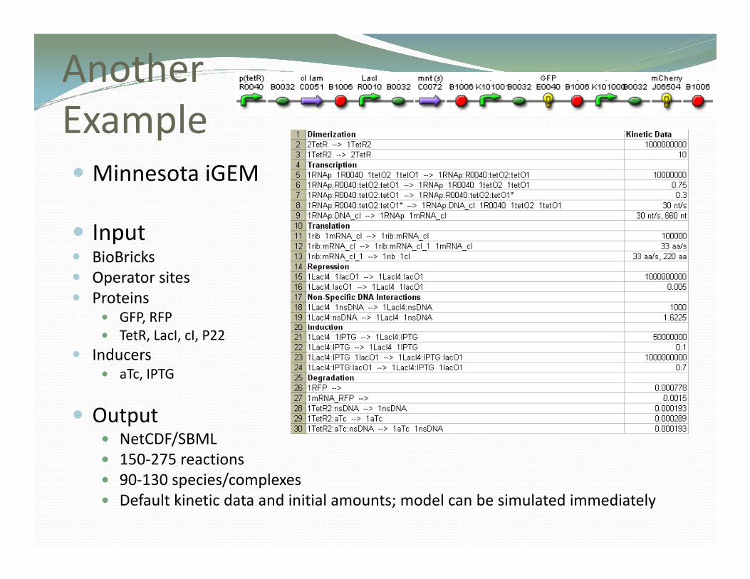
AnotherE lExample
Minnesota iGEMMinnesota iGEM
InputBi B i kBioBricksOperator sitesProteins
GFP, RFPTetR, LacI, cI, P22
InducersaTc, IPTG
OutputNetCDF/SBML150‐275 reactions90‐130 species/complexesDefault kinetic data and initial amounts; model can be simulated immediately

SynBioSS WikiSynBioSS WikiAddresses the problem of finding suitable kinetic data
Built on MediaWiki
C h h i bi l d bConnects to other synthetic biology databases:BioBricks, NCBI, PDB, SABIO‐RK
Select biochemical compounds
Automatically build models for simulation
Languages used in SynBioSS Wiki: PHP, SQL, HTML, Javascript, AJAX, DHTML, XML, MathML, SBML
// / / /Available at http://neptune.cems.umn.edu/wiki/index.php/Main_Page

SynBioSS Wiki

DatabaseDatabase
MySQL database management system
Two SectionsStandard MediaWiki tables
Custom tablesS iSpecies
Reactions
We have already stored information regarding components of the tetracycline, lactose, arabinose and l bd hlambda phage operons.

iSpeciesTypes
Complex, DNA/RNA, Lipids, Proteins, Small Molecules (e.g. ATP)ATP)
Unique IdentifiersCASCAS
GenBank
NCBI
PDB
PubMed
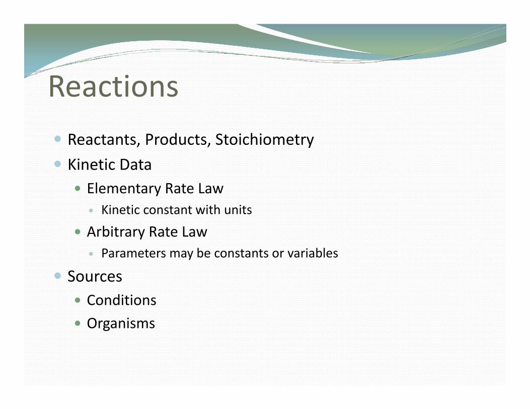
R iReactions
Reactants, Products, Stoichiometry
Kinetic DataElementary Rate Law
Kinetic constant with units
Arbitrary Rate LawArbitrary Rate LawParameters may be constants or variables
SourcesConditions
Organisms
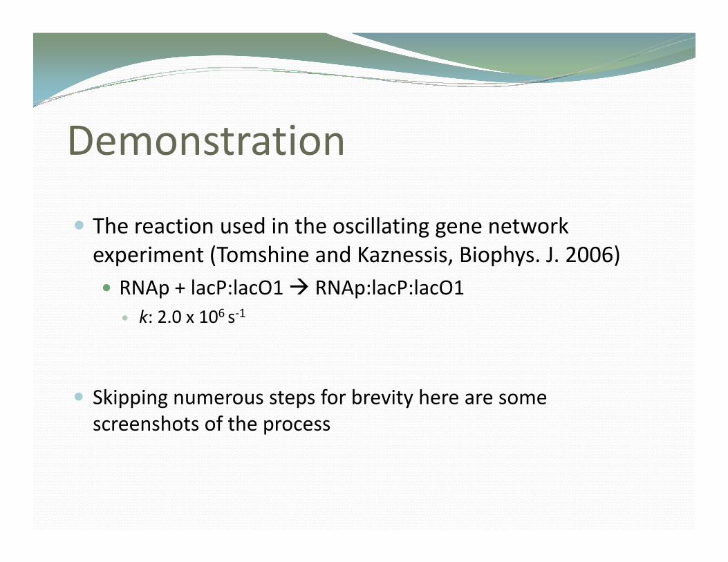
Demonstration
The reaction used in the oscillating gene network ( )experiment (Tomshine and Kaznessis, Biophys. J. 2006)
RNAp + lacP:lacO1 RNAp:lacP:lacO1k: 2 0 x 106 s‐1k: 2.0 x 10⁶ s 1
Skipping numerous steps for brevity here are some screenshots of the process

Add a Speciesdd a Spec es

Add a Speciesdd a Spec es

Add a Speciesdd a Spec es

Add a Reactiondd a eact o
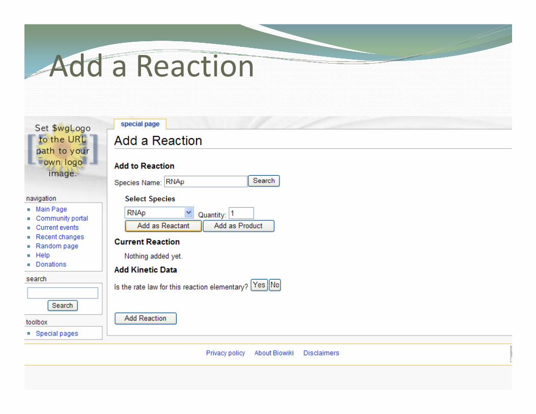
Add a Reactiondd a eact o

Add a Reactiondd a eact o

Add a Reactiondd a eact o

Add a Reaction [ ] [ ]x yv a b=dd a eact o
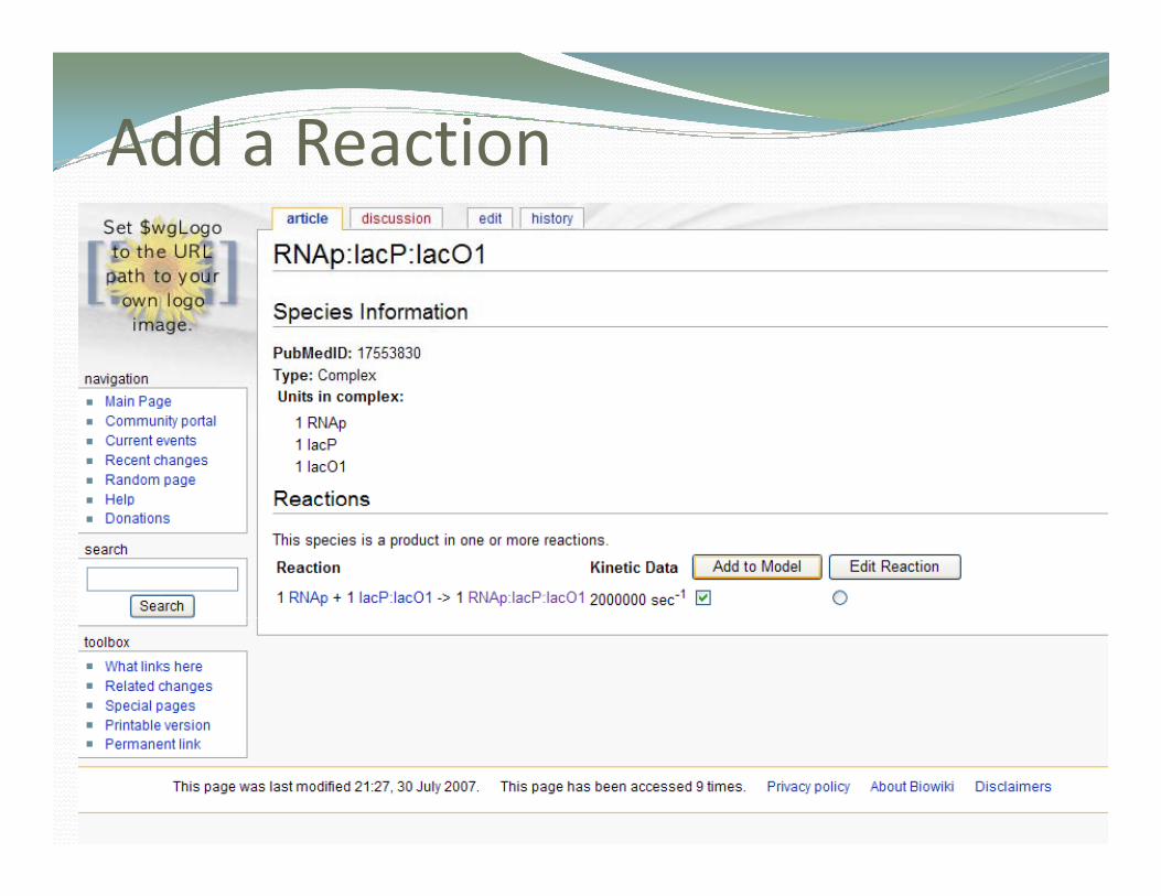
Add a Reactiondd a eact o

Custom ModelCusto ode
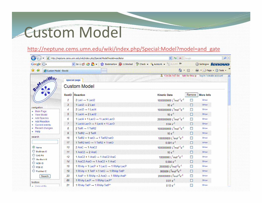
Custom ModelCusto odehttp://neptune.cems.umn.edu/wiki/index.php/Special:Model?model=and_gate


Computational Synthetic BiologyComputational Synthetic BiologyComputational Synthetic BiologyComputational Synthetic Biology
• How can we use SynBioSS to rationalize synthetic biology?
• Model gene networks with all the known molecular• Model gene networks with all the known molecular components.
• Generate detailed design principles.
Tuttle, Salis, Tomshine, Kaznessis, Biophys. J. (2005)Salis, Kaznessis, Phys. Biol. (2007)Tomshine and Kaznessis, Biophys. J. (2006)Sotiropoulos Kaznessis BMC Systems Biology (2007)Sotiropoulos, Kaznessis, BMC Systems Biology, (2007)Kaznessis, BMC Systems Biology, (2007)
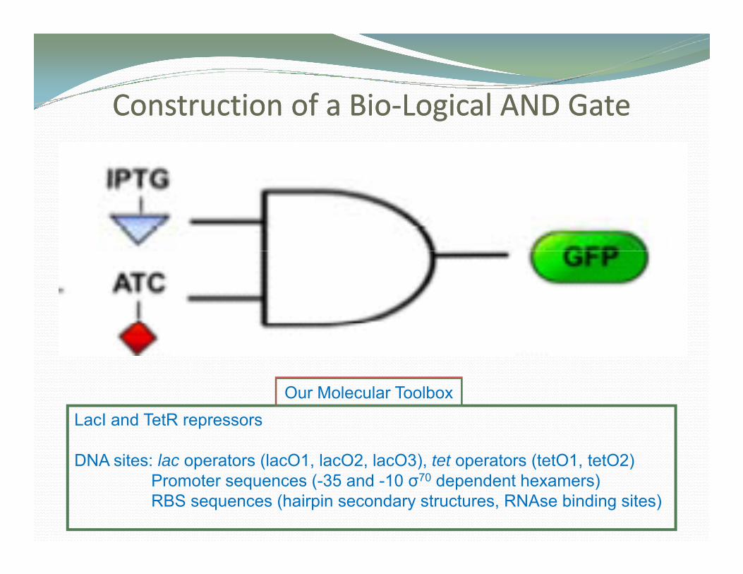
Construction of a BioConstruction of a Bio‐‐Logical AND GateLogical AND GateConstruction of a BioConstruction of a Bio‐‐Logical AND GateLogical AND Gate
Our Molecular ToolboxOur Molecular ToolboxLacI and TetR repressors
DNA sites: lac operators (lacO1, lacO2, lacO3), tet operators (tetO1, tetO2)p ( , , ), p ( , )Promoter sequences (-35 and -10 σ70 dependent hexamers)RBS sequences (hairpin secondary structures, RNAse binding sites)

AND Logic GGate
Express a gene whenExpress a gene when two signals are present:
aTc
IPTG
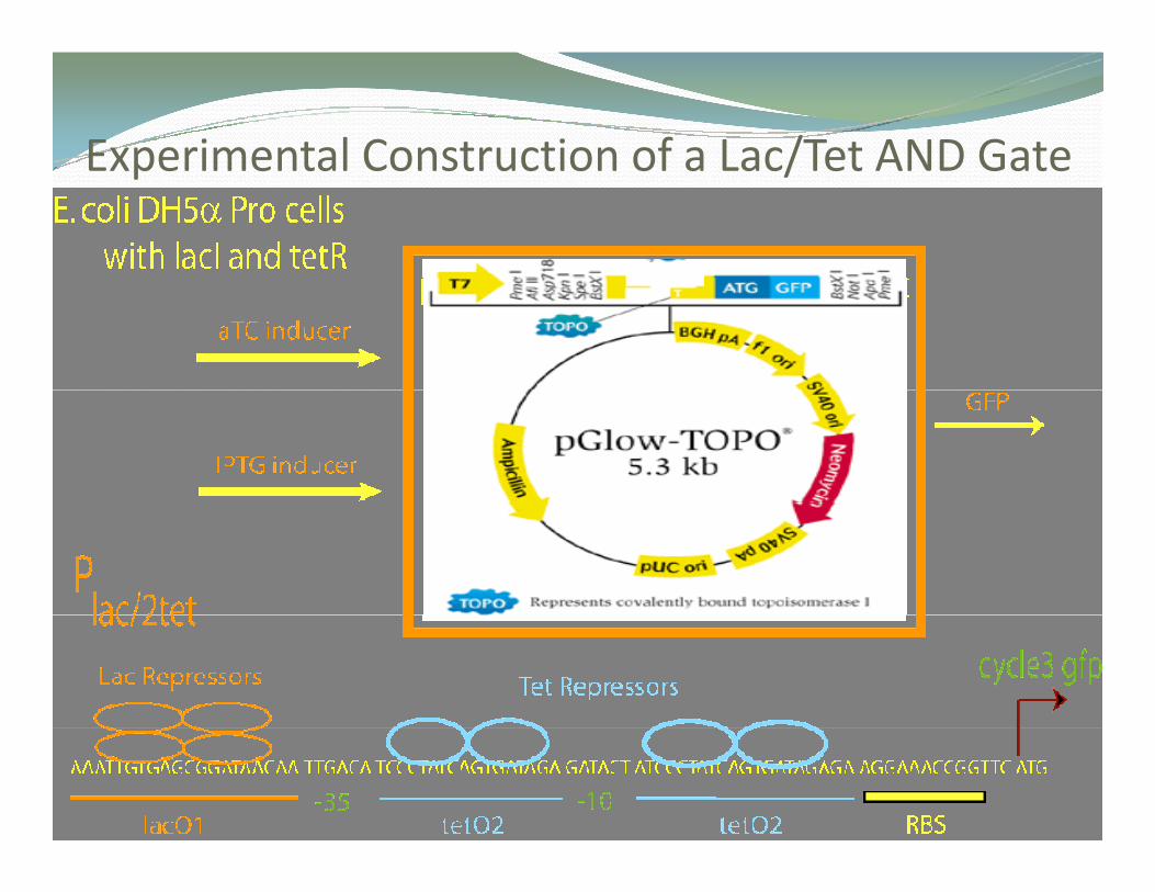
Experimental Construction of a Lac/Tet AND GateExperimental Construction of a Lac/Tet AND Gate

Models/Experiments Based on Models/Experiments Based on
i
Real Real BiomolecularBiomolecular ComponentsComponents
Plac O1 lacZ O2 lacYACAPO3PI lacI
LacR tetramer repressor protein
O1PlaclacI lacI
-1162 bp -82 bp -61bp +10 bp +411 bp
Inducer: lactose or IPTG
lac
Lac operon
tetAO1 O2tetR
TetR dimer repressor protein
O1 O2tetR
PAPR1
PR2
Inducer: tetracycline
PR1
PR2
Tet operony

dimerizationdimerizationReaction NetworkReaction Network
RNAp TetR and RNAp
++2 TetR1 → TetR2 TetR2 → 2 TetR1
TetR2 + tetO2 → TetR2:tetO2 TetR2:tetO2 → TetR2 + tetO2 RNAp TetR and RNApRNAp
P O2 lac
TetR and RNAp(un)binding
TetR2:tetO2 → TetR2 + tetO2
RNAp + tetP → RNAp:tetPRNAp:tetP → RNAp + tetP
RNAp
P O2 lac
TetR and RNAp(un)binding
Opening of DNA, TranscriptionOpening of DNA, Transcription
RNAp:tetP → RNAp:tetP* tetO2 + RNAp:tetP* → tetP + RNAp:tetO2
RNAp:tetO2 → RNAp + tetO2 RNAp:tetO2 → tetO2 + RNAp:DNA lac
RNApRNAp
P O2 lacP O2 lac
RNApRNAp:tetO2 tetO2 RNAp:DNA_lacRNAp:DNA_lac → RNAp + mRNA_lac
rib + mRNA_lac → rib:mRNA_lacrib:mRNA_lac → mRNA_lac + rib:mRNA_lac1 ib RNA l 1 L R1 + ib + D
mRNA_lac
Translation+mRNA_lac
Translation+
mRNA_lacrib:mRNA_lac1 → LacR1 + rib + Dara
RNase + mRNA_lac → RNase:mRNA_lacRNase:mRNA_lac → RNase
Degradation of proteins and mRNADegradation of proteins and mRNADTet→ TetR1 → TetR2 →

Model Structure: Network

AND Gate SimulationsAND Gate SimulationsAND Gate SimulationsAND Gate SimulationsRxn# Reaction k Ref. Rxn# Reaction k Ref. Rxn# Reaction k Ref.
1 2 LacR1 --> LacR2 1.00E+09 A 31 2 TetR1 --> TetR2 1.00E+09 d 51 2 AraC1 --> AraC2 1.00E+09 d 2 LacR2 --> 2 LacR1 1.00E+01 A 32 TetR2 --> 2 TetR1 1.00E+01 d 52 AraC2 --> 2 AraC1 1.00E+01 d 3 2LacR2 >LacR4 100E+09 A 33 TetR2 +tetO1 >TetR2:tetO1 286E+06 F 53 AraC2 +araO2 >AraC2:araO2 100E+07 He•Species are uniformly distributed in the cell.3 2 LacR2 --> LacR4 1.00E+09 A 33 TetR2 + tetO1 --> TetR2:tetO1 2.86E+06 F 53 AraC2 + araO2 --> AraC2:araO2 1.00E+07 He 4 LacR4 --> 2 LacR2 1.00E+01 A 34 TetR2:tetO1 --> TetR2 + tetO1 3.76E-02 F 54 AraC2:araO2 --> AraC2 + araO2 4.00E-03 H e 5 LacR4 + lacO1 --> LacR4:lacO1 5.00E+09 B 35 TetR2 + tetO2 --> TetR2:tetO2 2.98E+06 F 55 RNAp + araP --> RNAp:araP 2.00E+08 I e 6 LacR4:lacO1 --> LacR4 + lacO1 3.85E-04 B 36 TetR2:tetO2 --> TetR2 + tetO2 2.13E-02 F 56 RNAp:araP --> RNAp + araP 6.00E-02 I e 7 LacR4 + lacO2 --> LacR4:lacO2 5.00E+09 B 37 RNAp + tetP --> RNAp:tetP 8.60E+05 G 57 RNAp:araP --> RNAp:araP* 1.67E-02 I 8 LacR4:lacO2 --> LacR4 + lacO2 3.85E-04 B 38 RNAp:tetP --> RNAp + tetP 1.00E-01 G 58 araO2 + RNAp:araP* --> araP + RNAp:araO2 1.00E-01 I
•Initial cell volume is ~10-15 L
C ll di i i 30 5 i t th
Reference Key: A. Levandowski et. al., 1996 B. Gilbert and Müller-Hill, 1970p p p p
9 LacR4 + lacO3 --> LacR4:lacO3 5.00E+09 B 39 RNAp:tetP + tetO1 --> tetP + RNAp:tetO1 1.30E-02 G 59 RNAp:araO2 --> RNAp + araO2 5.77E-04 d 10 LacR4:lacO3 --> LacR4 + lacO3 3.85E-04 B 40 RNAp:tetO1 + tetO2 --> RNAp:tetO2 + tetO1 3.00E+01 C 60 RNAp:araO2 --> araO2 + RNAp:DNA_lac 3.00E+01 C 11 lacP + RNAp --> RNAp:lacP 2.00E+06 B 41 RNAp:tetO2 --> tetO2 + RNAp:DNA_ara 3.00E+01 C 61 RNAp:DNA_lac --> RNAp + mRNA_lac 30, 600 C 12 RNAp:lacP --> lacP + RNAp 1.00E-02 B 42 RNAp:DNA_ara --> RNAp + mRNA_ara 30, 660 C 62 rib + mRNA_lac --> rib:mRNA_lac 1.67E-01 b 13 lacO1 + RNAp:lacP --> lacP + RNAp:lacO1 1.00E-02 B 43 mRNA_ara + rib --> rib:mRNA_ara 1.67E-01 b 63 rib:mRNA_lac --> mRNA_lac + rib:mRNA_lac1 1.00E+02 D
•Cell division occurs every 30+5 minutes: the volume doubles exponentially and then halves.
•Simulate a grid of 6x6 aTc IPTG pair
1970 C. Vogel and Jensen, 1994 D. Sorensen and Pedersen, 1991 E. Elowitz and Leibler, 2000
14 RNAp:lacO1 --> lacO1 + RNAp 5.77E-04 a 44 rib:mRNA_ara --> mRNA_ara + rib:mRNA_ara1 1.00E+02 D 64 rib:mRNA_lac1 --> LacR1 + rib + Dara 100, 600 D 15 RNAp:lacO2 --> lacO2 + RNAp 5.77E-04 a 45 rib:mRNA_ara1 --> rib + Dtet + AraC1 100, 660 D 65 RNase + mRNA_lac --> RNase:mRNA_lac 1.50E-02 b 16 RNAp:lacO3 --> lacO3 + RNAp 5.77E-04 a 46 mRNA_ara + RNase --> RNase:mRNA_ara 1.50E-02 b 66 RNase:mRNA_lac --> RNase 1.00E+15 b 17 lacO2 + RNAp:lacO1 --> lacO1 + RNAp:lacO2 3.00E+01 C 47 RNase:mRNA_ara --> RNase 1.00E+15 b 67 Dara --> 3.85E-04 c 18 lacO3 + RNAp:lacO2 --> lacO2 + RNAp:lacO3 3.00E+01 C 48 Dtet --> 3.85E-04 c 68 LacR1 --> 2.31E-03 E 19 l O4 +RNA l O3 >l O3 +RNA l O4 300E+01 C 49 A C1 > 193E04 c 69 L R2 > 231E03 E
•Simulate a grid of 6x6 aTc-IPTG pair concentrations (0-200 ng/ml and 0-2mM).
•Simulate 1 000 trajectories for each pair
F. Kędracka-Krok and Wasylewski, 1999 G. Bertrand-Burggraf et. al., 1984 H. Stickle et. al.., 199419 lacO4 + RNAp:lacO3 --> lacO3 + RNAp:lacO4 3.00E+01 C 49 AraC1 --> 1.93E-04 c 69 LacR2 --> 2.31E-03 E
20 RNAp:lacO4 --> lacO4 + RNAp 5.77E-04 C 50 AraC2 --> 1.93E-04 c 70 LacR4 --> 2.31E-03 E 21 RNAp:lacO4 --> lacO4 + RNAp:DNA_tet 3.00E+01 C 22 RNAp:DNA_tet --> RNAp + mRNA_tet 30, 660 C 23 rib + mRNA_tet --> rib:mRNA_tet 1.67E-01 b 24 rib:mRNA tet -->mRNA tet +rib:mRNA tet1 1.00E+02 D
Simulate 1,000 trajectories for each pair.
• Simulate six designs (LLT, TTL).
H. Stickle et. al.., 1994 I. Zhang et. al.., 1996
rib:mRNA_tet mRNA_tet + rib:mRNA_tet1 1.00E+02 D25 rib:mRNA_tet1 --> rib + Dlac + TetR1 100, 660 D 26 RNase + mRNA_tet --> RNase:mRNA_tet 1.50E-02 b 27 RNase:mRNA_tet --> RNase 1.00E+15 b 28 Dlac --> 3.85E-04 c 29 TetR1 --> 2.31E-03 E
•Measure GFP number of molecules for 216,000 trajectories (36,000 CPU hours).

Design and SimulateDesign and Simulate
LTT
TLTTLT
TTL

SYNTHETIC SYNTHETIC PROMOTER DESIGNSPROMOTER DESIGNS
LTT
TLT
TTL
P

Flow Flow cytometrycytometryy yy y
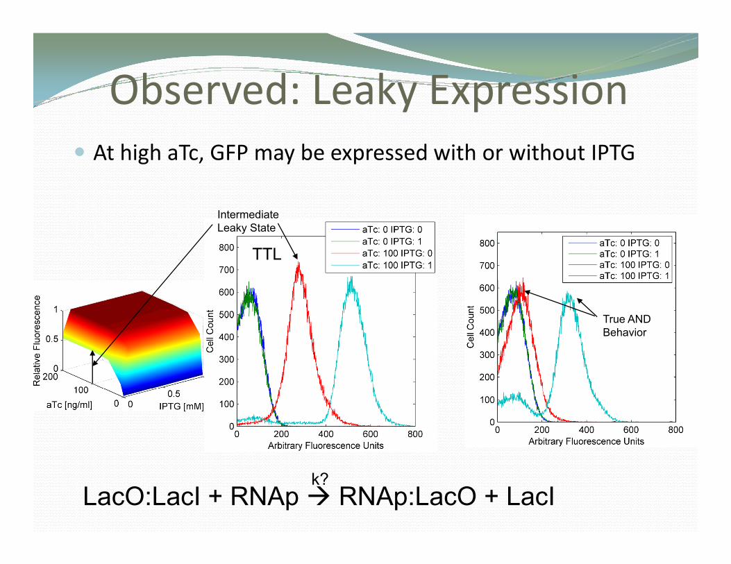
Observed: Leaky ExpressionObse ed ea y p ess oAt high aTc, GFP may be expressed with or without IPTG
Intermediate Leaky State
TTL LTT
True ANDTrue AND Behavior
k?LacO:LacI + RNAp RNAp:LacO + LacI

Biological InsightBiological InsightBiological InsightBiological Insight
• In the first model there was no leakinessIn the first model there was no leakiness.•One parameter fitted for each design.
RNAp + lacP + lacI4:lacO1 + tetO1 + tetO2 → RNAp:lacP + lacI4 + tetO1 + tetO2

ComputerComputer‐‐AidedAidedDesignDesign ofof BioBio‐‐LogicalLogicalDesignDesign ofof BioBio LogicalLogicalANDAND GatesGates
•Models assist in the design of synthetic biological systems.
•TTL is the highest‐fidelity And gate.
• Leakage of lacO can explain the variable phenotypic behavior Biological insightbehavior. Biological insight.

SummarySummarySu a ySu a y
Available toolbox of DNA sequences and regulatory proteins.Available toolbox of DNA sequences and regulatory proteins. Design novel gene networks to control protein production.
Hybrid stochastic‐discrete and stochastic‐continuous networkHybrid stochastic discrete and stochastic continuous network simulations tackle multiple scales.
Software tool available to the synthetic and systems biologySoftware tool available to the synthetic and systems biology community (Hy3S and SynBioSS).http://synbioss.sourceforge.net/
Computer‐assisted design of a synthetic Bio‐Logical AND‐gate.
Modeling can generate design principles for rational biological engineering.