computational techniques in animal breedingnce.ads.uga.edu/~ignacy/ads8200/course08.pdf ·...

Computational techniques inanimal breeding

by Ignacy Misztal

University of GeorgiaAthens, USA

First Edition Sept 1999Last Updated June 4, 2008

2

Contents

Preface . . . . . . . . . . . . . . . . . . . . . . . . . . . . . . . . . . . . . . . . . . . . . . . . . . . . . . . . . . . . . . . . . . . . . . 5

Software engineering . . . . . . . . . . . . . . . . . . . . . . . . . . . . . . . . . . . . . . . . . . . . . . . . . . . . . . . . . . . 7

Fortran . . . . . . . . . . . . . . . . . . . . . . . . . . . . . . . . . . . . . . . . . . . . . . . . . . . . . . . . . . . . . . . . . . . . . . 9Fortran 90 - Basics . . . . . . . . . . . . . . . . . . . . . . . . . . . . . . . . . . . . . . . . . . . . . . . . . . . . . 10Compiling . . . . . . . . . . . . . . . . . . . . . . . . . . . . . . . . . . . . . . . . . . . . . . . . . . . . . . . . . . . . 24Advanced features in Fortran 95 . . . . . . . . . . . . . . . . . . . . . . . . . . . . . . . . . . . . . . . . . . . 26

General philosophy of Fortran 90 . . . . . . . . . . . . . . . . . . . . . . . . . . . . . . . . . . . . 37Fortran 2003 . . . . . . . . . . . . . . . . . . . . . . . . . . . . . . . . . . . . . . . . . . . . . . . . . . . . . . . . . . . 45Parallel programming and OpenMP . . . . . . . . . . . . . . . . . . . . . . . . . . . . . . . . . . . . . . . . 46Rewriting programs in F77 to F95 . . . . . . . . . . . . . . . . . . . . . . . . . . . . . . . . . . . . . . . . . 50

Setting-up mixed model equations . . . . . . . . . . . . . . . . . . . . . . . . . . . . . . . . . . . . . . . . . . . . . . 53Fixed 2-way model . . . . . . . . . . . . . . . . . . . . . . . . . . . . . . . . . . . . . . . . . . . . . . . . . . . . . . 53

Extension to more than two effects . . . . . . . . . . . . . . . . . . . . . . . . . . . . . . . . . . . 56Computer program . . . . . . . . . . . . . . . . . . . . . . . . . . . . . . . . . . . . . . . . . . . . . . . . 58

Model with covariables . . . . . . . . . . . . . . . . . . . . . . . . . . . . . . . . . . . . . . . . . . . . . . . . . . 60Nested covariable . . . . . . . . . . . . . . . . . . . . . . . . . . . . . . . . . . . . . . . . . . . . . . . . . 62Computer program . . . . . . . . . . . . . . . . . . . . . . . . . . . . . . . . . . . . . . . . . . . . . . . 63

Multiple trait least squares . . . . . . . . . . . . . . . . . . . . . . . . . . . . . . . . . . . . . . . . . . . . . . . . 65Missing traits . . . . . . . . . . . . . . . . . . . . . . . . . . . . . . . . . . . . . . . . . . . . . . . . . . . . 69Different models per trait . . . . . . . . . . . . . . . . . . . . . . . . . . . . . . . . . . . . . . . . . . . 70Example of ordering by models and by traits . . . . . . . . . . . . . . . . . . . . . . . . . . . 70Computer program . . . . . . . . . . . . . . . . . . . . . . . . . . . . . . . . . . . . . . . . . . . . . . . 72

Mixed models . . . . . . . . . . . . . . . . . . . . . . . . . . . . . . . . . . . . . . . . . . . . . . . . . . . . . . . . . 76Popular contributions to random effects - single trait . . . . . . . . . . . . . . . . . . . . . 76Numerator relationship matrix A . . . . . . . . . . . . . . . . . . . . . . . . . . . . . . . . . . . . . 77Rules to create A-1 directly . . . . . . . . . . . . . . . . . . . . . . . . . . . . . . . . . . . . . . . . . . 78Unknown parent groups . . . . . . . . . . . . . . . . . . . . . . . . . . . . . . . . . . . . . . . . . . . . 79Numerator relationship matrix in the sire model . . . . . . . . . . . . . . . . . . . . . . . . . 80Variance ratios . . . . . . . . . . . . . . . . . . . . . . . . . . . . . . . . . . . . . . . . . . . . . . . . . . . 82Covariances between effects . . . . . . . . . . . . . . . . . . . . . . . . . . . . . . . . . . . . . . . . 84Random effects in multiple traits . . . . . . . . . . . . . . . . . . . . . . . . . . . . . . . . . . . . . 84

Multiple traits and correlated effects . . . . . . . . . . . . . . . . . . . . . . . . . . . . 85Computer pseudo-code . . . . . . . . . . . . . . . . . . . . . . . . . . . . . . . . . . . . . . . . . . . . 87

Storing and Solving Mixed Model Equations . . . . . . . . . . . . . . . . . . . . . . . . . . . . . . . . . . . . . . . 92Storage of sparse matrices . . . . . . . . . . . . . . . . . . . . . . . . . . . . . . . . . . . . . . . . . . . . . . . . 93

Ordered or unordered triples . . . . . . . . . . . . . . . . . . . . . . . . . . . . . . . . . . . . . . . . 93IJA . . . . . . . . . . . . . . . . . . . . . . . . . . . . . . . . . . . . . . . . . . . . . . . . . . . . . . . . . . . . 93

3

Linked lists . . . . . . . . . . . . . . . . . . . . . . . . . . . . . . . . . . . . . . . . . . . . . . . . . . . . . . 94Trees . . . . . . . . . . . . . . . . . . . . . . . . . . . . . . . . . . . . . . . . . . . . . . . . . . . . . . . . . . . 95Summing MME . . . . . . . . . . . . . . . . . . . . . . . . . . . . . . . . . . . . . . . . . . . . . . . . . . 96

Searching algorithms . . . . . . . . . . . . . . . . . . . . . . . . . . . . . . . . . . . . . . . . . . . . . . . . . . . . 97Numerical methods to solve a linear system of equations . . . . . . . . . . . . . . . . . . . . . . . . 99

Gaussian elimination . . . . . . . . . . . . . . . . . . . . . . . . . . . . . . . . . . . . . . . . . . . . . . 99LU decomposition (Cholesky factorization) . . . . . . . . . . . . . . . . . . . . . . . . . . . 100

Storage . . . . . . . . . . . . . . . . . . . . . . . . . . . . . . . . . . . . . . . . . . . . . . . . . . . . . . . . . . . . . . 102Triangular . . . . . . . . . . . . . . . . . . . . . . . . . . . . . . . . . . . . . . . . . . . . . . . . . . . . . . 102Sparse . . . . . . . . . . . . . . . . . . . . . . . . . . . . . . . . . . . . . . . . . . . . . . . . . . . . . . . . . 102Sparse matrix inversion . . . . . . . . . . . . . . . . . . . . . . . . . . . . . . . . . . . . . . . . . . . 104Numerical accuracy . . . . . . . . . . . . . . . . . . . . . . . . . . . . . . . . . . . . . . . . . . . . . . 106

Iterative methods . . . . . . . . . . . . . . . . . . . . . . . . . . . . . . . . . . . . . . . . . . . . . . . . . . . . . . 107Jacobi . . . . . . . . . . . . . . . . . . . . . . . . . . . . . . . . . . . . . . . . . . . . . . . . . . . . . . . . . 108Gauss-Seidel and SOR . . . . . . . . . . . . . . . . . . . . . . . . . . . . . . . . . . . . . . . . . . . . 108Preconditioned conjugate gradient . . . . . . . . . . . . . . . . . . . . . . . . . . . . . . . . . . . 110Other methods . . . . . . . . . . . . . . . . . . . . . . . . . . . . . . . . . . . . . . . . . . . . . . . . . . 111

Convergence properties of iterative methods . . . . . . . . . . . . . . . . . . . . . . . . . . . . . . . . . 111Properties of the Jacobi iteration . . . . . . . . . . . . . . . . . . . . . . . . . . . . . . . . . . . . 116Properties of the Gauss-Seidel and SOR iterations . . . . . . . . . . . . . . . . . . . . . . 116Practical convergence issues . . . . . . . . . . . . . . . . . . . . . . . . . . . . . . . . . . . . . . . 116Determination of best iteration parameters . . . . . . . . . . . . . . . . . . . . . . . . . . . . 117

Strategies for iterative solutions . . . . . . . . . . . . . . . . . . . . . . . . . . . . . . . . . . . . . . . . . . . 117Solving by effects . . . . . . . . . . . . . . . . . . . . . . . . . . . . . . . . . . . . . . . . . . . . . . . . 117Iteration on data (matrix-free iteration) . . . . . . . . . . . . . . . . . . . . . . . . . . . . . . . 118Indirect representation of mixed-model equations . . . . . . . . . . . . . . . . . . . . . . . 121

Summary of iteration strategies . . . . . . . . . . . . . . . . . . . . . . . . . . . . . . . . . . . . . . . . . . . 126

Variance components . . . . . . . . . . . . . . . . . . . . . . . . . . . . . . . . . . . . . . . . . . . . . . . . . . . . . . . . . 127REML . . . . . . . . . . . . . . . . . . . . . . . . . . . . . . . . . . . . . . . . . . . . . . . . . . . . . . . . . . . . . . 127General Properties of Maximization Algorithms . . . . . . . . . . . . . . . . . . . . . . . . . . . . . . 133

Some popular maximization algorithms . . . . . . . . . . . . . . . . . . . . . . . . . . . . . . 136Acceleration to EM (fixed point) estimates . . . . . . . . . . . . . . . . . . . . . . . . . . . . 139Convergence properties of maximization algorithms in REML . . . . . . . . . . . . 142Accuracy of the D and DF algorithms . . . . . . . . . . . . . . . . . . . . . . . . . . . . . . . . 144

Method R . . . . . . . . . . . . . . . . . . . . . . . . . . . . . . . . . . . . . . . . . . . . . . . . . . . . . . . . . . . . 147Bayesian methods and Gibbs sampling . . . . . . . . . . . . . . . . . . . . . . . . . . . . . . . . . . . . . 153

Using the Gibbs sampler . . . . . . . . . . . . . . . . . . . . . . . . . . . . . . . . . . . . . . . . . . 159Multiple-traits . . . . . . . . . . . . . . . . . . . . . . . . . . . . . . . . . . . . . . . . . . . . 161Convergence properties . . . . . . . . . . . . . . . . . . . . . . . . . . . . . . . . . . . . . 162

Ways to reduce the cost of multiple traits . . . . . . . . . . . . . . . . . . . . . . . . . . . . . . . . . . . . . . . . . 165Canonical transformation . . . . . . . . . . . . . . . . . . . . . . . . . . . . . . . . . . . . . . . . . . . . . . . . 165

4

Canonical transformation and REML . . . . . . . . . . . . . . . . . . . . . . . . . . . . . . . . 167Numerical properties of canonical transformation . . . . . . . . . . . . . . . . . . . . . . . 168Extensions in canonical transformation . . . . . . . . . . . . . . . . . . . . . . . . . . . . . . . 169

Multiple random effects . . . . . . . . . . . . . . . . . . . . . . . . . . . . . . . . . . . . . 169Missing traits . . . . . . . . . . . . . . . . . . . . . . . . . . . . . . . . . . . . . . . . . . . . . 170Different models per trait . . . . . . . . . . . . . . . . . . . . . . . . . . . . . . . . . . . . 171

Implicit representation of general multiple-trait equations . . . . . . . . . . . . . . . . . . . . . . 173

Computing in genomic selection . . . . . . . . . . . . . . . . . . . . . . . . . . . . . . . . . . . . . . . . . . . . . . . . 177

Data manipulation . . . . . . . . . . . . . . . . . . . . . . . . . . . . . . . . . . . . . . . . . . . . . . . . . . . . . . . . . . . 179Renumbering . . . . . . . . . . . . . . . . . . . . . . . . . . . . . . . . . . . . . . . . . . . . . . . . . . . . . . . . . 179Memory consideration . . . . . . . . . . . . . . . . . . . . . . . . . . . . . . . . . . . . . . . . . . . . . . . . . . 179Look-up tables . . . . . . . . . . . . . . . . . . . . . . . . . . . . . . . . . . . . . . . . . . . . . . . . . . . . . . . . 180Sort and merge . . . . . . . . . . . . . . . . . . . . . . . . . . . . . . . . . . . . . . . . . . . . . . . . . . . . . . . 181Data manipulation options . . . . . . . . . . . . . . . . . . . . . . . . . . . . . . . . . . . . . . . . . . . . . . 188

Unix utilities . . . . . . . . . . . . . . . . . . . . . . . . . . . . . . . . . . . . . . . . . . . . . . . . . . . 189

Sources and References . . . . . . . . . . . . . . . . . . . . . . . . . . . . . . . . . . . . . . . . . . . . . . . . . . . . . . . 191

5

Preface

These notes originated as class notes for a graduate-level course taught at the University ofGeorgia in 1997. The goal of that course was to train students to program new ideas in animalbreeding. Programming was in Fortran because Fortran programs are relatively easy fornumerical problems, and many existing packages in animal breeding that are still useful werewritten in Fortran. Since the computer science department at UGA does not teach courses inFortran any longer, the first few lectures were devoted to Fortran 77 and then to Fortran 90. Allprogramming examples and assignments were in Fortran 90. Because the students had onlylimited experience in programming, the emphasis was on generality and simplicity even at someloss of efficiency.

Programming examples from the course led to an idea of a general yet simple BLUP programthat can be easily modified to test new methodologies in animal breeding. An integral part of thatprogram was a sparse matrix module that allowed for easy but efficient programming of sparsematrix computations.

The resulting program was called BLUPF90 and supported general multiple trait models withmissing traits, different models per trait, random regressions, separate pedigree files anddominance. An addition of a subroutine plus a minor change in the main program convertedBLUPF90 to REMLF90 - an accelerated EM variance-component program, and BLUP90THR - abivariate threshold-linear model. An addition of subroutines created a Gibbs sampling programGIBBSF90. I greatly appreciate collaborators who contributed to the project. Tomasz Strabeladded a dense-matrix library. Shogo Tsuruta created extensions of in-memory program toiteration-on-data. Benoit Auvray added estimation of thresholds to the threshold model programs. Monchai Duanginda, Olga Ravagnolo, and Deuhwan Lee worked on adding threshold andthreshold-linear model capability to GIBBSF90.Shogo Tsuruta and Tom Druet worked onextension to AI-REML. Tom Druet wrote an extension to Method R, which can work with largedata sets.... Indirect contributions were made by Andres Legarra and Miguel Perez-Enciso...

Program development of BLUPF90 and the other programs was not painless. Almost every f90compiler had bugs, and there were many small bugs in the programs. As Edison wrote, “ thesuccess is 1% inspiration and 99 perspiration.” Now the programs are already useful but there isroom for improvements.

The programming work took time away from the notes, so the notes are far from complete. Notall ideas are illustrated by numerical examples or sample programs. Many ideas are too sketchy,and references are incomplete. Hopefully the notes will become better with time..... I am gratefulto all who have reported errors in the notes, and particularly to Dr. Suzuki from ObihiroUniversity and his group.

Developing good programs in animal breeding is a work for more than one person. There aremany ideas around how to make them more comprehensive and easier to use. I hope that the

6

ideas presented in the notes and expressed in the programs will be helpful to many of you. Inreturn, please share your suggestions for improvement as well as programming developmentswith me and the animal breeding community.

Ignacy MisztalJuly 1998 - May 2008

7

Software engineering

In programming, we are interested in producing quality code in a short period of time. If thatcode is going to be used over and over again, and if improvements will be necessary, also clarityand ease of modification are important.The following steps are identified in software engineering:

Step Purpose Example

Requirements Description of the problem tobe solved

Variance component estimation forthreshold animal models

Specifications Specific description withdetailed limits on what theprogram should do

Number of equations up to 200,000;number of effects up to 10; thefollowing models are supported;line-mode code (no graphics);computer independent.Generation of test examples.

Design Conceptual program (e.g., inpseudo-code) where allalgorithms of the program havebeen identified

Estimates by accelerated EM-REML, mixed models set up bylinked list, sparse matrixfactorization. Pseudo-code (or flowdiagram) follows .

Possibly a program in very high-level, e.g., SAS IML or Matlab(prototyping)

Coding Writing code in a programminglanguage

Implementation in Fortran 90

Testing Assurance that the programmeets the specifications

Validation Assurance that the programmeets the requirements

In commercial projects, each of these step is documented so that many people can work on thesame project, and that departure of any single person won’t destroy the project.

For small programming projects, it appears that only the coding step is done. In fact, the othersteps are done also conceptually, just not documented.

8

It is important that all of the above steps are understood and done well. Changes to earlier stepsdone late are very expensive. Jumping right into programming without deliberation onspecifications and design is a recipe for disaster!

In research programs where many details are not known in advance, programming may take along time, and final programs may contain many mistakes that are not discovered until after thepaper has been accepted or a degree has been awarded.

One possible step towards simpler programing is by reduction of program complexity by usingvery high-level language. In a technique called prototyping, one would first write a program in avery high-level but possibly inefficient language (SAS, Matlab, R, AWK,..). This assures that theproblem has been understood and delivers executed examples, and in the end can cut drasticallyon coding and testing!

Another way of reducing the cost of programming is using “object-oriented” programming,where complicated operations are defined as easily as possible, and complicated (but efficient)code is “hidden” in application modules or classes. This way, one can approach the simplicity ofa matrix language with an efficiency of Fortran or C. This approach, using Fortran 90, isfollowed in the notes and in project BLUPF90.

LiteratureRoger. S. Pressman. 1987. Software Engineering. McGraw Hill.

Computational Cost

Let n be a dimension of a problem to solve, for example a size of the matrix.If for large n cost ~ a f(n) then computational complexity is O[f(n)]

Algorithms Name ExampleO(n) linear Reading dataO[nlog(n)] log-linear SortingO(n2) quadratic Summing a matrixO(n3) cubic Matrix multiplicationO(2n) exponential exhaustive search

Algorithms usually have separate complexity for memory and computations. Often a memory-efficient algorithm is inefficient in computations and vice versa.Desirable algorithms are linear or log-linear. A fast computer is generally not a substitute for apoor algorithm for serious computations.

ObservationAdvances in computing speed are evenly due to progress in hardware and in algorithms.

9

Fortran

For efficient implementation of mathematical algorithms, Fortran is still the language of choice. A few standards are coexisting:

Fortran 77 (F77) with common extensions,Fortran 90 (F90).Fortran 95 (F95)

The standard for F90 includes all F77 but not necessarily all the extensions. While F90 addsmany new features to F77, changes in F95 as compared to F90 are small although quite useful. Plenty of high-quality but often hard to use software is available for F77. On the other hand,programs written in F90/F95 are simpler to write and easier to debug. The best use of old F77subroutines is to “encapsulate” them into much-easier to use but just efficient F90 subroutines.

The next chapter provides a very basic overview of F90. The subsequent chapter is partly aconversion guide from F77 to F90 and partly an introduction to more advanced features of F90and F95. There is also a chapter on converting old programs in F77 to F95.

Only the most useful and “safe” features of F90 and F95 are covered. For a more detaileddescription of Fortran, read regular books on F90/95 programming.

10

Fortran 90 - Basics

Example program

! This is a simple example

program test! program for testing some basic operationsimplicit noneinteger:: a,b,c!read*,a,bc=a**b !exponentiationprint*,’a=’,a,’b=’,b,’a**b=’,c! Case is not important PRINT*,’a**b=’,Cend

Rules:- program starts with optional statement “program”, is followed by declarations and endswith “end”

- case is not important except in character strings- text after ! is ignored and treated as comment; comments are useful for documentation

VariablesVariables start with letters and can include letters, numbers and character “_”. Examples: a, x, data1, first_month

Data typesinteger 4 byte long, range approx. -2,000,000,000 - 2,000,000,000

Guaranteed range is 9 decimal digits

real 4 byte floating point with accuracy of about 7 digits and range of about10-34 - 1034. Examples: 12.4563, .56e-10

real (r8) (r8 to be defined) ordouble precision

8 byte floating point with accuracy of 15 digits and range of about10-300 - 10300. Examples: 12.4563, .56d-10

11

logical - 4 bytes, values of .true. or .false.character (n) - a character string n characters long. One byte = one character.

Examples: ‘abcdef’, “qef”, “we’ll”. Strings are either single ‘’or doublequotes “ ”. If a string is enclosed in double quotes, single quotes inside aretreated as normal characters, and vice versa.

complex not used much in animal breeding; see textbooks

InitializationVariables can optionally be initialized during declaration; without declarations, they holdundetermined values (some compilers initialize some variables to equivalents of integer 0; thisshould not be relied on).

Examples

implicit noneinteger::number_effect=5, data_pos,i=0,jreal::value,x,y,pi=3.1415character (10)::filename=’data.run2000'logical::end_of_file, file_exists=.false.

If a line is too long, it can be broken with the & symbol:

integer::one, two, three,& four, five

Warning:An undeclared variable in F90 is treated as integer if its name starts with “i-n” and as realotherwise. A statement: ‘implicit none’ before declarations disables automaticdeclarations. Always use ‘implicit none’before declaring your variables. Declaration ofall variables (strong typing) is an easy error-detection measure that requires a few extraminutes but can save hours or days of debugging.

implicit noneinteger::a,b,c....

.....

Arrays

12

integer::x(2,100) integer array with 2 rows and 100 columnscharacter(5)::x(10) character array of 10 elements, each 5-character long real:: c(3,4,5) 3-D array of 60 elements total

By default, indexing of each element of an array starts with 1. There are ways to make it startfrom any other number.

Parameter (read-only) variables

integer,parameter:: n=5, m=20real,parameter::pi=3.14159265! parameter variables can be used to indicate dimensions in declarationsreal::x(n,m)

Operations on variables

ExpressionsNumerical expressions are intuitive except that ** stands for exponentiation.Fortran does automatic conversions between integers and reals. This sometimes causesunexpected side effects

real::xinteger::i=2,j=4x=i*j/10print*,’i*j/10',x !This prints 0, why?!x=i*j/10.0print*,’i*j/10.0=',x !This print 0.8end

With matrices, operation involving a scalar is executed separately for each matrix element:real::x(3)x=1 !all elements of x set to 1x(1)=1; x(2)=4; x(3)=7x=x*5 !all elements of x multiplied by 5

Character manipulationscharacter (2)::a=’xy’,bcharacter (10)::ccharacter (20)::dc=’pqrs'

13

b=ac=a//b//c//’123' !catenationd=c(3:4) !d is equal ‘rs'

Basic control structures

IF statement

if (condition) statement ! statement is executed only if condition is true

if (condition) then ! as above but can contain many statements .....endif

If statements can contain many conditions using elseif. If no condition is fulfilled, an elsekeyword can be used.

if (condition1) then ! ..... ! executed if condition1 is true elseif (condition2) .... ! executed if condition2 is true elseif(condition3)

.... .... else .... !optional; executed when none of previous conditions are trueendif

Conditions in if

< <= == (equal) >= > /= (not equal).and. .not. .or.

! IF examplereal::xread*,xif (x >5 .and. x <20) then print*,’number geater than 5 and smaller than 20' elseif (x<0) then print*,’ x smaller than 0:’,x

14

endifend

Select case statement

These statements are optimized for conditions based on integer values

select case ( 2*i) !expression in () must be integer or charactercase( 10)

print*, 10 case (12:20,30)

print*,'12 to 20 or 30' case default !everything else, optional

print*, 'none of 10:20 or 30' end select

Loops

Statements inside the loop are executed repeatedly, until some termination condition occurs. Inthe simplest loop below, statements inside the loop below are executed for i=1,2,...,n

do i=1,n !basic do loop .....enddo

The example below shows creation and summation of all elements of a matrix in a do loop

integer::,i,jinteger,parameter::n=10real::x(n,n),sumx!c! initialize the matrix to some values, e.g., x(i,j)=i*j/10do i=1,n do j=1,n x(i,j)=i*j/10.0 enddoenddo!! now total

15

sumx=0do i=1,n do j=1,n sumx=sumx+x(i,j) enddoenddoprint*,sumx!!can do the same using fortran90 function sum()print*,sum(x)

Indices in loops can be modified to count with a stride other than one and even negative

do j=5,100,5 !j =5,10,15,...,100...do k=5,1,-1 !k=5,4,..,1...

Another loop operates without any counter. An exit statement ends the loop.

do .....if (x==0) exit......

end do

x=1 do ! no condition mandatory

x=x*2 if (x==8) cycle ! skip just one iterationif (x>=32) exit ! quit the loopprint*,x

end do

Functions and subroutines

!Program that calculates trace of a few matricesinteger,parameter::n=100real::x(n,n),y(n,n),z(n.n),tr

......! trace calculated in a loop

16

tr=0do i=1,n tr=tr+x(i,i)enddo!! trace calculated in a subroutine; see body of subroutine belowcall trace_sub(tr,x,n)

! trace calculated in a function; see body of function belowtr=trace_f(x,n)end

subroutine trace(t,x,n)integer::n,ireal x(n,n),t!t=0do i=1,n t=t+x(i,i)enddoend

function trace(x,n) result(t)integer::n,ireal:x(n,n),t!

t=0do i=1,n t=t+x(i,i)enddoend

In a subroutine, each argument can be use as input, output, or both. In a function, all argumentsare read only, and the “result: argument is write only. Functions can simplify programs becausethey can be part of an arithmetic expression

! example with subroutine call trace(t,x,n)y=20*t**2+5

!example with a function

17

y=20*trace_f(x,n)+5

Subroutines and functions are useful if similar operations need to be simplified, or a largeprogram decomposed into a number of smaller units.

Argument passingIn a subroutine, each variable can be read or written. In a program:

call trace(a,b,m)...subroutine trace(t,x,n)a and t are pointing to the same storage in memory. Same with b and x, and m and n. In somecases, no writing is possible:

call trace (a,b,5) !writing to p either does not work or changes constant 5call trace(x, y+z, 2*n+1) ! expressions cannot be changed

Save featureOrdinarily, subroutines and functions do not “remember” variables inside them from one call toanother. To cause them to remember, use the “save” statement.

function abcd(x) result(y)...integer,save::count=0 !keeps count; initialized to 0 first time onlyreal,save::old_x !keeps previous value of x....count=count+1old_x=xend

Without save, the variables are initialized the first time only, and on subsequent calls haveundetermined values.

“return” from the middle of a subroutine or function:

subroutine ..........if (i > j) return...end

18

Intrinsic (built-in) functionsFortran contains large number of predefined functions. More popular are:

int - truncating to integer nint - rounding to integerexp, log, log10abs - absolute valuemod - modulomax - maximum of possibly many variablesminsqrt - square rootsin,cos,tanlen - length of character variable

INPUT/OUTPUT

General statements to read or write are read/write/print statements. The command:

print*,a,b,cprints a,b and c on the terminal using a default format. Variables in the print statement can includevariables, expressions and constants. These are valid print statements:

print*,’the value of pi is ‘,3.14159265print*,’file name =’,name,’ number of records =’,nrec

Formatted print uses specifications for each printed item. Formatted print would be print ff,a,b,c

where ff contains format specifications. For example:print ‘(5x,”value of i,x,y =”,i4,2x,f6.2,f6.2)’,i,x,y

Assuming i=234, x=123.4567 and y=0.9876, this prints: value of i,x,y = 234 123.46 0.99

Selected format descriptions

i5 integer five characters wide

a5 character 5 characters wide

a character as wide as the variable(character a*8 would read as a8)

19

f3.1 3 characters wideOn write, 1 digit after commaOn read, if no comma read as if last 1 digit after comma (123 read as 12.3, 1 as .1) if real with comma, read as is (1.1 read as 1.1, .256 read as .256)

5x On write, output five spacesOn read, skip five characters

‘text’‘’text’‘

On write only, output string ‘text’use double quotes when format is a character variable or string

/ Skip to next line

Shortcuts (i5,i5,i5) / ‘(3i5)’‘(i2,2f5.1, i2,2f5.1)’ / ‘(2(i2,2f5.1))’

Example

print ’(i3,”squared=”,i5)’,5,25

This prints: 5 squared= 25

Character variables can be used for formatting:

character(20)::ff...ff=’(i3,’‘ squared=’’,i5)’print ff,5,25

Reading from a keyboard is similar in structure to writing:read*,a,b,c !default, sometimes does not work with alphanumeric variablesread ff,a,b,c !ff contains format

Reading from files and writing to files

File operations involve units, which are integer numbers. To associate unit 2 with a file:open(2,file=’/home/abc/data_bbx’)

Read and write from/to file has a syntax:read(2,ff)a,b

20

write(2,ff)a,b

Formats can be replaces by * for default formatting. Units can be replaced by * for reading fromkeyboard or writing to keyboard. Thus:

read(*,*)a,b !read from keyboard using defaultsread*,a,b ! identical to above simplified

and write(*,*)a,b,c !write to keyboard using defaultsprint*,a,b,c !identical to above simplified

are equivalent.

To read numerical data from file bbu_data using default formattinginteger::acharacter (2)::breal::x!! open file “bbu-data” as unit 1open (1,file=’bbu_data’)

! read variables from that file in free format and then print themread(1,*)a,b,xprint*,a,b,x! asterisk above denotes free format!! read same variables formatted rewind 1read(1,’(i5,a2,f5.2)’)a,b,x

In most fortran implementations, unit 5 is preassigned to keyboard and unit 6 to console. “Print”statement prints to console. Thus, the following are equivalent:

write(6,’(i3,’‘ squared=’’,i5)’)5,25and

print ’(i3,’‘ squared=’’,i5)’, 5,25

Also these are equivalent:read(5,*)x

andread*,x

Free format for reading the character variables does not always work. One can use the following

21

from the keyboard:

read (5,’(a)’)stringor

read ‘(a)’,string

Attention: One read statement generally reads one line whether all characters have been reador not! Thus, the next read statement cannot read characters that the previous onehas skipped.

Assume file “abc” with contents:1 2 34 5 67 8 9

By default, one read statement reads complete records. If there is not enough data in one record,reading continues to subsequent records.

integer::x, y(4)open(1,file=’abc’)

read(1,*)xprint*,xread(1,*)yprint*,yend

produces the following14 5 6 7

Implied loop

The following are equivalent:

integer::x(3),i! statements below are equivalentread*,x(1),x(2),x(3)read*,xread*,(x(i),i=1,3)

Implied loops can be nested

integer::y(n,m),i,j

22

read*,((y(i,j),j=1,m),i=1,n)

! statement below reads by columnsread*,x! and is equivalent toread*,((y(i,j),i=1,n),j=1,m) !note reversal of indices; orread*,((y(:,j),j=1,m)

Implied loop is useful in assignment of values to arrays

real::x(n,n),d(n)integer::cont(100)!d=(/(x(i,i),i=1,n)/) !d contains diagonal of xcont=(/(i,i=1,100)/) !cont contains 1 2 3 4 ... 100

Detection of end of files or errors

integer::statusread(...,iostat=status)if (status == 0) then print*,’read correct

else print*,’end of data’endif

Unformatted input/output

Every time a formatted I/O is done, the programs performs a conversion from character format tocomputer internal format (binary). This takes time. Also, an integer or real variable can use up to10 characters (bytes) in formatted form but only 4 bytes in binary, realizing space savings. Sincebinary formats in different computers and compilers may be different, data files in binary usuallycannot be read on other systems.

Unformatted I/O statements are similar to formatted ones except that the format field is omitted.

real x(1000,1000)open(1,file=’scratch’,form=’unformatted’).......write(1)x

23

....rewind 1read(1)x.....rewind 1write(1)m,n,x(1:m,1:n) !writing and reading section of a matrix....rewind 1read(1)m,n,x(1:m,1:n)....close(1,status=’delete’)end

Statement CLOSE is needed only if the file needs to be deleted, or if another file needs to beopened with the same unit number.

Reading from/to variables

One can read from a variable or write to a variable. This may be useful in creating names offormats. For example:

character (20)::ff write(ff, ‘(i2)’)i ff=’(‘ // ff // ’f10.2)’ !if i=5, ff=’( 5f10.2)’

The same can be done directly: write(ff, ‘( “(“, i2, ”f10.2)” )’ )i ! spaces only for clarity

Reading/writing with variables always require a format, i.e., * formatting does not work.

24

Compiling

Programs in Fortran 90 usually use the suffix f90. To compile program pr.f90 on a Unix system,type: f90 pr.f90where f90 is the name of the fortran 90 compiler. Some systems use a different name.

To execute, type:a.out

To name the executable pr rather than default a.out:f90 -o pr pr.f90

To use optimizationf90 -O -o pr pr.f

Common options:-g add debugging code-static or -s compile with static memory allocation for subroutines that includes

initializing memory to 0; use for old programs that don’t work otherwise.

Hints

If a compile statement is long, e.g.,f90 -C -g -o mm mm.f90

to repeat it in Unix under typical conditions (shell bash or csh), type!f

If debugging a code is laborious, and the same parameters are typed over and over again, put themin a file, e.g., abc, and type:

a.out <abc

To repeat, type!a

Programs composed of several units are best compiled under Unix by a make command. Assumethat a program is composed of three units: a.f90, b.f90 and c.f90. Create a file called Makefile asbelow:

a.out: a.o b.o c.of90 a.o b.o c.o

a.o: a.f90

25

f90 -c a.f90

b.o: b.f90f90 -c b.f90

c.o: c.f90f90 -c c.f90

After typingmake

all the programs are compiled and linked into an executable. Later, if only one program changes,typing

makecauses only that program to be recompiled and all the programs linked. The make command has alarge number of options that allows for high degree of automation in programming.

Attention: Makefile requires tabs after : and in front of commands; spaces do not work!

26

Advanced features in Fortran 95

This section is a continuation of the previous chapter that introduces more advanced features ofF95. This section also has some repetitive information from the former section to also be anupgrade guide from F77.

Free and fixed formatsFortran 77 programs in traditional fixed format are supported, usually as files with suffix “.f”.Fixed format programs can be modified to include features on the f90 fortran. Free formatprograms usually have suffix “.f90".

Free format (if suffix .f90)! Comments start after the exclamation mark! One can start writing at column 1 and continue as long as convenient!integer:: i1, i2, i3, j1, j2, j3,& !integer variables k1, k2, m, n !& is line continuation symbol

real :: xx !XX is name of the ! coefficient matrix

&,yy !if continuation is broken by a blank or comment, use & as here

a=0; b=0 !multiple statements are separated by semicolon

Long namesUp to 32 characters

New names for operators == (.eq.), /= (.ne.), <=, =>, <, >

Matrix operations real :: x(100,100),y(100,100),z(100),v(20),w(20),p(20,20),a...x(:,l)=y(l,:)p=x(21:40,61:80) ! matrix segmentsv=z(1:100:5) ! stride of 5: v=(/z(1), z(6),z(11),...,z(96)/)v=x(10:100:10,1:10)**5 ! operation with a constanty=matmul(z,y) ! matrix multiplicationp=x(:20,81:) ! same as x(1:20,81:100)print*,sum(z(1,:)x=transpose(y) !x=y’print*,dot_product(v,w) !v’w

27

a=maxval(x) ! maximum value in xprint*,count(x>100) ! number of elements in x that satisfy the conditiona=sum(y) ! sum of all elements of yprint*,sum(y,dim=1) ! vectors that contains sums by rowprint*,sum(y,mask=y>2.5) ! sum of all elements > 0.5

See other functions like maxloc(), any(), all(),size....

Vector and matrix operations involve conformable matrices

Constructorsreal :: x(2),y(1000),g(3,3)...x=(/13.5,2.7/) !x(1)=3.5, x(2)=2.7y=(/ (i/10.0, i=l,l000) /) !y=[.1 .2 .3 ... 99.9 100]...i=2; j=5x=(/i**2,j**2/) ! constructors may include expressions; x=[4 25]y(1:6)=(/x,x,x/) ! constructors may include arrays

g(:,1)=(/1 2 3/); g(:,2)=(/4,5,6/); g(:,3)=(/7,8,9/) ! matrix initialized by columnsg=reshape( (/1,2,3,4,5,6,7,8,9/), (/3,3/) ) ! matrix initialized by reshape()

Constructors can be used in indices!

integer::i(2), p(10)...i=(/2,8/)...p(i)=p(i)+7 !p(2)=p(2)+7, p(8)=p(8)+7

New declarations with attributes integer,parameter::n=10,m=20 ! parameters cannot be changed in the programreal,dimension(n,m)::x,y,z ! x, y and z have the same dimension of n x m

real::x(n,m),y(n,m),z(n,m) ! equivalent to above

real (r4),save::z=2.5 ! Real variable of precision r4 with value saved (in a subroutine)character (20):: name ! character 20 bytes long

28

New control structuresselect case ( 2*i) !expression in () must be integer or character

case( 10) print*, 10

case (12:20,30) print*,'12 to 20 or 30'

case default print*, 'none of 10:20 or 30'

end select

x=1 do ! no condition mandatory

x=x*2 if (x==8) cycle ! skip just one iterationif (x>=32) exit ! quit the loopprint*,x

end do

real:: x(100,1000) where (x >500)

x=0 !done on all x(i)>500 elsewhere

x=x/2 end where

Allocatable arrays

real,allocatable::a(:,:) ! a declared as 2-dimensional arrayallocate (a(n,m)) ! a is now n x m array..if (allocated(a)) then ! the status of allocatable array can be verified

deallocate(a) ! memory freedendif

Pointer arrays

29

real,pointer::a(:,:),b(:,:),c(:,:),d(:) ! a-c declared as 2-dimensional arraysallocate (a(n,m)) ! a is now n x m array

b=>a ! b points to a, no copy involvedc=>a ! a-c point to the same storage location

allocate(a(m,m)) !a points to new memory; nullify (b) !association of b eliminatedb=null() ! same as above

allocate(b(m,m)b=a !b copied to a

deallocate(c) !deallocate memory initially allocated to ac=>b(1:5,1:10:2) !pointer can point to section of a matrixd=>b(n,:) !vector pointer pointing to a row of a matrix

if (associated(b)) then ! test of association deallocate(b) ! memory freed and b nullified

endif

real,target::x(2,3) !pointer can point to non-pointer variables with target attributereal,allocatable,target::y(:,:)real::pointer::p1(:,:,p2(:,:)...p1=>xp2=>y

Read more on pointers later.

Data structures type animal

character (len= 13) :: id,parent(2) integer :: year_of birth real :: birth weight,weaning weight

end type animal

type (animal) :: cow...read( 1 ,form)cow%id,cow%sire,cow%dam,cow%yob,cow%bw,cow%ww

To avoid typing the type definitions separately in each subroutine, put all structure definitions in a

30

module, e.g., named definitions

module aa type animal...end typetype ......end type

end module

Program mainuse aa !use all definitions in the module type(animal): :cow...end

subroutine pedigreeuse aatype(animal): :cow...end

To include modules in the executable file: 1) compile files containing those modules, 2) if modules are not in the same directory as programs using them, use appropriate compile

switch, 3) if modules contains subroutines, the object code of the modules needs to be linked.

Elements of data structures can be pointers (but not allocatable arrays) and can be initialized.

type sparse_matrix integer::n=0 integer,pointer::row(:)=>null(),col(:)=null() real,pointer::val(:)=>null()end type

Automatic arrays in subroutinesreal:: x(5,5)..call sub1(x,5)...

31

subroutine sub1(x,n)real:: x(n,n),work(n,n) !work is allocated automatically and deallocated on exit..end

New program organization - internal functions/subroutines and modulesFunctions and subroutines as described in the previous section are separate program units. Theycan be compiled separate from main programs and put into libraries. However, there are prone tomistakes as there is no argument checking, e.g., subroutines can be called with wrong number ortype of arguments without any warning during compilation.

Fortran 90 allows for two new possibilities for placement of procedures: internal within a programand internal within a module.

! This is a regular program with separate proceduresprogram abcd...call sub1(x,y)...z=func1(h,k)end program

subroutine sub1(a,b)....end subroutine

function func1(i,j)....end function

! This is the same program with internal subroutinesprogram abcd...call sub1(x,y)...z=func1(h,k)

contains ! end program is moved to the end and “contains” is inserted

subroutine sub1(a,b) ....

32

end subroutine function func1(i,j) ..... end function

end program

Internal procedures have access to all variables of the main program. Procedures internal to theprogram cannot be part of a library.

! This program uses modulesmodule mm1 contains subroutine sub1(a,b) .... end subroutine function func1(i,j) ..... end functionend module

program abcduse mm1 !use module mm1...call sub1(x,y)...z=func1(h,k)end program

An example of internal functions or subroutinesprogram abcinteger :: n=25real :: x(n)...call abc(i)

contains

subroutine abc(i) integer ::i

33

... if (i<=n) x(i)=0 !variables declared in the main program need not

! be declared in internal subroutines end subroutine...end program

Procedures that are internal or contained within modules can have special features that make them simpler or more convenient to use.

Deferred size arrays in subroutines or functions real:: x(5,5)..call sub1(x)...

subroutine sub1(x)real:: x(:,:) !size is not specified; passed automaticallyreal::work(size(x,dim=1),size(x,dim=2)) !new variable created with dimension of x()..end subroutine

This works only if the program using the subroutine sub1 is informed of its arguments, either by (1) preceding that program by an interface statement, (2) by putting sub1 in a module and usingthe module in the program, or 3) by making the subroutine an internal one. .

(1)interface subroutine sub1(a) real::a(:,:) end subroutineend interfacereal::x(5,5)....

(2)module abc interface

34

subroutine sub1(x) real:: x(:,:) real::work(size(x,dim=1),size(x,dim=2)) .. endend module

program mainuse abcreal::x(5,5).....end program

(3)program mainreal::x(5,5)..... contains

subroutine sub1(x) real:: x(:,:) real::work(size(x,dim=1),size(x,dim=2)) .. end subroutineend program

Use of interface statements results in interface checking, i.e., whether arguments in subroutinecalls and actual subroutines agree.

The module can be compiled separately from the main program. The module should be compiledbefore it is used by a program.

Function returning arrays

A function can return an array. This array can be either deferred size if its dimensions can bededuced from the function arguments, or it can be a pointer array.

function kronecker1(y,z) result(x)!this function returns y “kronecker product” zreal::y(:,:),z(:,:), z(size(y,dim=1)*size(z,dim=1), size(y,dim=2)*size(z,dim=2))...end function

35

function kronecker2(y,z) result(x)!this function returns y “kronecker product” zreal::y(:,:),z(:,:)real,pointer:: z(:,:)..allocate(z(size(y,dim=1)*size(z,dim=1), size(y,dim=2)*size(z,dim=2))...end function

function consec(n) result (x)! returns a vector of [1 2 3 ... n]integer::n,x(n),i!x=(/(i,i=1,n)/)end function

Functions with optional and default parameterssubroutine test(one,two,three)integer, optional::one,two,threeinteger :: one1,two1,three1 !local variables !if (present(one)) then one1=one else one1=1endifif (present(two)) then two1=two else two1=2endifif (present(three)) then three1=three else three1=3 !endifprint*,one1,two1,three1end

.....

36

call test(l5,6,7)call test(10) !equivalent to call test(10,2,3)call test(5,three=67 ) !parameter three out of order

Subroutine/Function overloadingIt is possible to define one function that will work with several types of arguments (e.g., real andinteger). This is best done using modules and internal subroutines.

module prob!function rand(x) is a random number generator from a uniform distribution. ! if x is real - returns number in interval <0-x)! if x is integer - returns integer between 1 and x.

interface rand module procedure rand_real, rand_integer end interface

contains

function rand_real(x) result (y) real::x,y ! call random_number(y) !system random number generator in interval <0,1) y=y*x end function function rand_integer(x) result (y) integer::x,y real::z ! call random_number(z) !system random number generator in interval <0,1) y=int(y*z)+1 end function

end module

program overload!example of use of function rand in module prob

37

use prob !name of module where overloaded functions/subroutines are locatedinteger::nreal::x

! generate an integer random number from 1 to 100print*,rand(100)

! generate a real random number from 0.0 to 50.0print*,rand(50.0)end

Operator overloadingArithmetic operators (+ - / *) as well as assignment(=) can be overloaded, i.e., given differentmeaning for different structures.

For example,

Type (bulls):: bull_breed_A,&bull_breed_B,&bull_combined,& bull_different,& bull common

...!The following operations could be programmed

bull_combined = bull_breed_A + bull_breed_B bull_different = (bull_breed_A - bull_breed_B) + (bull_breed_B - bull_breed _ A) bull common = bull_breed_A * bull_breed_B

General philosophy of Fortran 90A fortran 90 program can be written in the same way as fortran 77, with the main program andmany independent subroutines. During compilation it is usually not verified that calls tosubroutines and the actual subroutines match. i.e., the number of arguments and their types match.With a mismatch, the program can crash or produce wrong results. Fortran 90 allows to organizethe program in a series of modules with a structure as follows:

MODULE m1interfacesdeclarations of data structuresdata declarations

38

CONTAINSsubroutines and functionsEND MODULE m1

MODULE m2interfacesdeclarations of data structuresdata declarations CONTAINSsubroutines and functionsEND MODULE m2

MODULE m3...

PROGRAM titleUSE MODULE m1,m2,..declarationsbody of main program CONTAINSinternal subroutines and functions END PROGRAM title

Each set of programs is in a module. If there is a common data to all programs together withcorresponding subroutines and functions, it can be put together in one module. Once a program(or a module) accesses a module, all the variables become known to that program and matching ofarguments is verified automatically.

It is a good practice to have each module in a separate file. Modules can be compiled separatelyand then linked. In this case, the compile line needs to include a directory where modules arecompiled.

Other selected features

New specifications of precision

integer,parameter::r4=selected_real_kind(6,30) ! precision with at least 6 decimal digits! and range of 1030

real(r4)::x ! x has accuracy of at least 6 digits (same as default)

39

integer,parameter::r8=selected_real_kind(15) ! as above but 15 decimal digits real(r8)::y ! y has accuracy of at least 15 decimal digits (same as double precision)

integer, parameter :: i2 = selected_int_kind( 4 ) ! integer precision of at least 4 digitsinteger, parameter :: i4 = selected_int_kind( 9 ) ! integer precision of at least 9 digits

To avoid defining the precision in each program unit, all definitions can be put into a module.

module kinds integer, parameter :: i2 = SELECTED_INT_KIND( 4 ) integer, parameter :: i4 = SELECTED_INT_KIND( 9 ) integer, parameter :: r4 = SELECTED_REAL_KIND( 6, 37 ) integer, parameter :: r8 = SELECTED_REAL_KIND( 15, 307 ) integer, parameter :: r16 = SELECTED_REAL_KIND( 18, 4931 ) integer, parameter :: rh=r8end module kinds

Variable i2 denotes precision of an integer with a range of at least 4 decimal digits or -10000 to10000. It usually can be a 2-byte integer. The variable i4 denotes precision of an integer with arange of at least 9 decimal digits. It can be a 4-byte integer. The variable r4 denotes precision of areal with the precision of at least 6 significant digit and a range of 1037. It can be a 4-byte real. Thevariable r8 denotes precision of a real with the precision of at least 15 significant digit and a rangeof 10307. It can be a 8-byte real. Finally rh is set to r8.

In a program

program testuse kindsreal (r4):: xreal (rh)::yinteger (i2)::a...end

Variables x,y, and a have appropriate precision. If variable y and other variables of precision rhneed to be changed to precision r4 to save memory, all what is needed is a change in the moduleand recompilation of the remaining programs.

Lookup of dimensions

real x(100,50)

40

integer p(2)

..print*,size(a) ! total number of elements(5000)print*,size(x,dim= 1) ! contains size of the first dimension (100) print*,size(x,dim=2) ! contains size of the second dimension (50)p=shape(x) ! p=(/100,50/)

Functions with results and intents

subroutine add (x,y,z)real, intent(in):: x ! x can be read but not overwrittenreal, intent(inout):: y ! y can be read and overwritten, this is defaultreal, intent(out):: z ! z cannot be read before it is assigned a value....end subroutine

Pointers II

The following example shows how a pointer variable can be enlarged while keeping the originalcontents and with a minimal amount of copying

real,pointer::p1(:),p2(:)

allocate(p1(100)) !p1 contains 100 elements.....! now p1 needs to contain extra 100 elements but with initial 100 elements intactallocate(p2(200))p2(1:100)=p1deallocate(p1)p1=>p2 ! now p1 and p2 point to the same memory locationnullify(p2) ! p2 no longer points to any memory location...end

If deallocate is not executed, memory initially assigned to p1 would become inaccessible. Carelessuse of pointers can result in memory leaks, where the amount of memory used is steadilyincreasing.

real,pointer::x(:)

41

do i=1,n x=>diagonal(y) ... deallocate(x) !memory leak if this line omittedenddo

Pointers can be used for creation of linked lists, where each extra element is added dynamically.

type ll_element real::x=0 integer::column=0 type (ll_element),pointer::next=>null()end type

type ll_matrix type(ll_element),pointer::rows(:)=>null() !pointer to each row of linked list integer::n=0 ! number of rowsend type

program maintype (ll_matrix)::xx !declaration...

Subroutine add_ll(a,i,j,mat)! mat(i,j)=mat(i,j)+atype (ll_matrix)::matreal::ainteger::i,jtype (ll_element)::current,last!current=>mat%rows(i) !points to first element in row ido

if (.not. associated(current) exit !exit loop to create new elementif (current%column == j) then

current%x=current%x+a !found element; add to itreturn !return from subroutine

elsecurrent=>current%next ! switch to next element and loop

enddo

!element not foundallocate(last)

42

current%next=>last !set link from the previous elementlast%column=j; last%x=a !set valuesend subroutine

Interfaces

operators (+,*,user defined)

One can create interfaces so that operations could look asa+bwhere a and b are structures of, say, type matrix.

The following would make it possible

interface operator (+) Module procedure addend interface contains

function add(x,y) result (z)type(matrix)::ztype(matrix), intent(in)::x,y...end function

In this casea+bhave the same effect asadd(a,b)

Please note that matrices being arguments of this function have “intent(in)”, i.e., the arguments ofthe function are defined as non-changeable. User defined operators need to be characters withinpoints, e.g. .add. or .combine. .

equal sign

To create an assignment that would bea=bcreate the following interface and function

interface assignment(=) Module procedure equalxy

43

end interface contains

subroutine equalxy(x,y)type(matrix),intent(out)::xtype(matrix), intent(in)::y...end function

Please note locations of intent(in) and intent(out). In this case, a=b

andcall equalab(a,b)

will result in identical execution.

Differences between Fortran 90 and 95

Fortran 95 includes a number of “fixes “ + improvements to F90. Some of them are shown here.

Timing function

The CPU timing function is now available as :

call cpu_time(x)

Automatic deallocation of allocatable arrays

Arrays allocated in procedures are automatically deallocated on exit.

Pointer and structure initialization

Pointers can be nullified when declared; most compilers but not all do it automatically.

real,pointer::x(:,:)=>null()

Elements of the structure can be initialized

44

type IJAinteger::n=0integer,pointer::,ia(:)=null(),ja(:)=nullreal,pointer::a(:)=null()

end type

Elemental subroutines

A subroutine/function defined as elemental for a scalar argument, can be automatically used witharrays. In this case, the same operation is performed on every element of the array.

real::x,y(10),z(5,5)

call pdf(x)call pdf(y)call pdf(z)..contains

elemental subroutine pdf(x)real::xx=1/(2*sqrt(3.14159265))*exp(-x**2/2)end subroutine

end program

In the program above, one can precalculate 1/(2*sqrt(3.14159265)) to avoid repeated calculations,but optimizing compilers do it automatically.

Many functions in Fortran 90 are elemental or seem to be elemental. This may include a uniformpseudo-random number generator.

real::x,y(12)!call random_number(x) ! x ~ un[0,1)call random_number (y) ! y(i)~un[0,1), i=1,12x=sum(y)-6 ! x ~ approx N(0,1)

Including the random_number subroutine as part of another elemental routine works well withsome compilers and generates errors (not pure subroutine) with others. In this case,random_number may be implemented as overloaded.

45

Fortran 2003

Specifications for Fortran 2003 are available, however, as of 2008 only some features of it areimplemented in selected compilers. Those described below are untested and should serve as general ideas. For a fuller description, search for “Features of Fortran 2003" on the Internet.

Automatic (re)sizing of allocatable matrices in expressions

real, allocatable::a(:,:), b(:,:),c(:,:),v(:)allocate (b(5,5),c(10,10))...a=b !a initialized as a(5:5)a=c !a deallocated and allocated as a(10,10)v(1:10)=b(1:2,1:5) ! V is allocated v(10)

New features for allocatable arrays

allocatable(a,source=b) !a gets attributes of bcall move_alloc(c,d) !c=d; d deallocated

“Stream” write/read. Variables are written as a sequence of bytes; reading can start from anyposition using the keyword POS.

open(1,access=’stream’)write(1)a,b,c,d !write variables as stream of bytesrewind 1read(1,pos=35)q !read starting from the byte 35 read(1,pos=10)z !read starting from byte 10

Asynchronous I/O. The program continues before the I/O is completed.

open(1,...,asynchronous=”yes”)do i=1,p

x=...write(1)x !no wait for write to finish

enddowait(1) !wait until all writing to unit 1finished

Many features of Fortran 2003 are for compatibility with the C language and for dynamicallocation of data structures and subroutines. For example, there is an ability to declare datastructures with variable precision.

type mat(kind,m,n)integer, kind::kindinteger,len::m,n

real(kind)::x(m,n)end type

type (mat(kind(0.0),10,20))::mat1 !mat1 is of single precisiontype (mat(kind(0.d0),10,20))::mat2 !mat2 is of double precision

46

Parallel programming and OpenMP

If a computer contains multiple processors, a program could potentially run faster if it is modifiedto use several processors. For any gains with parallel processing, the program needs to containsections that can be done in parallel. If a fraction of serial code that cannot be executed in parallelin a program is s, the maximum improvement in speed with parallel processing is 1/s.

A program running on several processors spends time on real computing plus on overhead ofparallel processing, which is data copying plus synchronization. When converting to parallelprocessing its is important that:

* The program still runs on a single processor without much performance penalty* Additional programming is not too complicated* Benefits are reasonable, i.e., small amount of time is spend in copying/synchronization* Extra memory requirements are manageable* Results are the same as with serial execution.

The parallel processing can be achieved in two ways: - automatically using a compiler option, - use of specific directives.

Both options require an appropriate compiler. The first option is usually quite successful forprograms that operate on large matrices. For many other programs, the program needs to bemodified to eliminate dependencies that would inhibit the possibility of parallel processing.

OpenMP

One of the most popular tools to modify an existing program for parallel processing is OpenMP.In this standard, extra directives (!$OMP....) are added to programs. In compilers that do notsupport OpenMP, these directives are ignored as comments. Several OpenMP constructs areshown below. Threads mean separately running program units; usually one thread runs on oneprocessor.

Everything inside these two directives is executed by all processors available.

!$OMP parallelprint*,”Hi” !will be printed many times, once per processor!$OMP end parallel

Any variable appearing in private() will be separate for each processor

!$OMP parallel private (x)call cpu_time(x)print*,x !will be printed many times once per processor

47

!$OMP end parallel

The loops will be distributed among processors available

!Variable i and any other loop counter are treated as separate! variables per processor!Each loop is assumed independent of each other; otherwise the! results may be wrong !$OMP dodo i=1,1000 ...end do!$OMP end do

Keyword “nowait” allows the second do loop section to execute before the first one is complete

!$OMP parallel!$OMP do do i=1

... enddo!$OMP end do nowait

!$OMP do do i=1,...

...!$OMP end do

Statements in each section are executed once all sections can be executed in parallel

!$OMP sections!$OMP section...!$OMP section...!$OMP section......!$OMP end section

Only the first thread to arrive executes the statements within while the other threads wait then skipthe statements.

!$OMP single...!$OMP end single

Only one thread can execute the statements at one time; the other threads need to wait before theycan execute them

!$OMP critical

48

...$OMP critical

No thread can proceed until all threads arive at this point

!$OMP barrier

Only one thread at a time can execute the statement below

!$OMP atomicx=x+....

Separate x are created for each thread; they are summed after the loop is complete.

$OMP do reduction (+:x)do i=...... x=x+...end do$OMP end do

Execute the following statements in parallel only if condition met; otherwise execution serial

!$OMP parallel if(n>1000)!$OMP......

OpenMP includes a number of subroutines and functions. Some of them are:

call MP_set_num_threads(t) - set number of threads to tOMP_get_num_procs() - number of processors assigned to program OMP_get_num_threads() - number of different processors actually activeOMP_get_thread_num() - actual number of thread (0 = main thread)OMP_get_wtime() - wall clock time

For example:

program testuse omp_libinteger::i,nprocreal::x!nproc=OMP_get_num_procs()!print*,nproc,” processors available”nproc=min(3,nproc) !use maximum 3 processors!call MP_set_num_threads(nproc) - set number of threads to nproc

49

!$OMP dodo i=1,10 print*,”iteration”,i,” executed by thread”,get_thread_num()enddo!$OMP end doend

Converting program from serial to parallel can take lots of programming and debugging.Additional issues involved are load balancing - making sure that all processors are busy- andmemory contention - that speed is limited by too much memory access. A useful information isgiven by compiler vendors, e.g., see PDF documents on optimizing and OpenMP of the IntelFortran compiler (http://www.intel.com/cd/software/products/asmo-na/eng/346152.htm) .

Given programming time, improving the computing algorithm may result in a faster and a simplerprogram than converting it to parallel. For examples, see Interbull bulletin 20 athttp://www-interbull.slu.se.

50

Rewriting programs in F77 to F95

The purpose of the rewrite is primarily simplification of old programs and not computing speed.In F77 it is very easy to make simple but hard-to-find programming mistakes while in F95 it ismuch more difficult. One can consider a rewrite or a “touch-up” when upgrade or fixes to an oldprogram are too time consuming or seem impossible.

The computing time in F95 may be longer due to management of memory allocation. However, ifa simpler program allows easy upgrade to a more efficient algorithm, the program in F95 mayend up being faster.

The complexity of the program is roughly the number of subroutines in a program times thenumber of arguments per subroutine, plus the number of declared variables times the size of code(excluding comments). A program can be simplified by:

1. deceasing the number of variables2. decreasing the number of subroutines3. decreasing the number of arguments per subroutine/function. 4. decreasing the length of the code (without using tricks)

The rewrite may be done at a few levels.

Simplest

Eliminate some loops by a matrix statement or a built-in functions p=0

do i=1,np=p+x(i)

enddo

p=sum(x(:n))

Compound functions! x~MVN(y,inv(z*p)).... ! multiply.... ! invert.... ! sample MVN(0,..).... ! add constant

x=normal(y,inv(mult(z,p))

Replace all work storage passed to subroutines with automatic arrays

51

real::work(n)...call mult(x,y,z,work,n)...subroutine mult(a,b,c,n)real::work(n) !work is used as

scratch

call mult(x,y,n)...

subroutine(x,y,n) real::work(n)

Possibly initialize variables in the declaration statement; beware of consequencesreal::a,b(20)integer::ja=0do i=1,20 b(i)=0end doj=0

real:a=0,b(20)=0integer:j=0!values initialized once

Use memory allocation to have matrices the right size and then eliminate separate bounds fordeclared and used indicesreal:x(10000)m=2*(n+7) ! used dimension of xcall comp(x,m,n)

real,allocatable:x(:)allocate (x(2*(n+7))call comp(x)

Level II

Simplify interfacing with old subroutines either by rewriting (if simple) or by reusing (writing aF95 interface); the rewritten subroutine as below must be either internal or in a module.call fact3dx(x,,n,m,w)...subroutine fact3dx(mat,n,m,work)! mat=fact(mat)integer::n,mreal::mat(n,n),work(n)...

call factor(x)......subroutine factor(mat)real::mat(:,:),w(size(mat,dim=1))interface subroutine fact3dx(mat,n,m,work) integer::n,m real::mat(n,n),work(n)end interfacecall fcat3dx(mat,size(w),size(w),w)end subroutine

Replace all “common” variables by a module

52

programinteger p(n)real x(m,m),z(n,n)common //p,x,z....subroutine aa...integer p(n)real x(m,m),z(n,n)common //p,x,z....

module stor integer p(n) real x(m,m),z(n,n)end module

program ..use stor

subroutine ..use stor

Change subroutines into internal subroutines (if specific to a program) or put them into module (ifsubroutines useful in other programs).

Level III

Replace old libraries by new, simpler to useOverload whatever makes senseOrganize variables into data structures

Level IV

Rewrite from scratch. The old program is utilized as a source of general algorithms and examples.

53

Setting-up mixed model equations

Good references on setting up models of various complexity are in Groeneveld and Kovacs(1990), who provide programming examples, and in Mrode (1996), who provides manynumerical examples and a large variety of models. The approach below provides both numericalexamples and programming. Almost all programming is in fortran 90, emphasizing simplicitywith programming efficiency. Fixed 2-way model

Mixed model: y = X$ + e. Assuming E(y)=X$, V(y)=V(e)=IF2, the estimate of $ is a solution

to normal equations:

Because X contains few nonzero elements and matrix multiplication is expensive (the cost iscubic), matrices X’X and X’y are usually created directly.

Datai j yij1 1 51 2 82 1 72 2 62 3 9

Write the model as yij = ai + bj + eij

The mixed model for the given data:

or

54

y = ( X1 + X2 + X3 + ... ) $ + e

Observation: first second third

One can write:

For the first two observations:

For a two-factor model, the contribution to X’X from one observation is always 4 elements ofones, in a square.

55

The contribution to X’y from one observation is always two elements with the values of thecurrent observation.

Rules

Define a function address(effect) that calculates the solution number corresponding to the i-theffect and the j-th level

Effect Address(effect)

a1 1

a2 2

b1 3

b2 4

b3 5

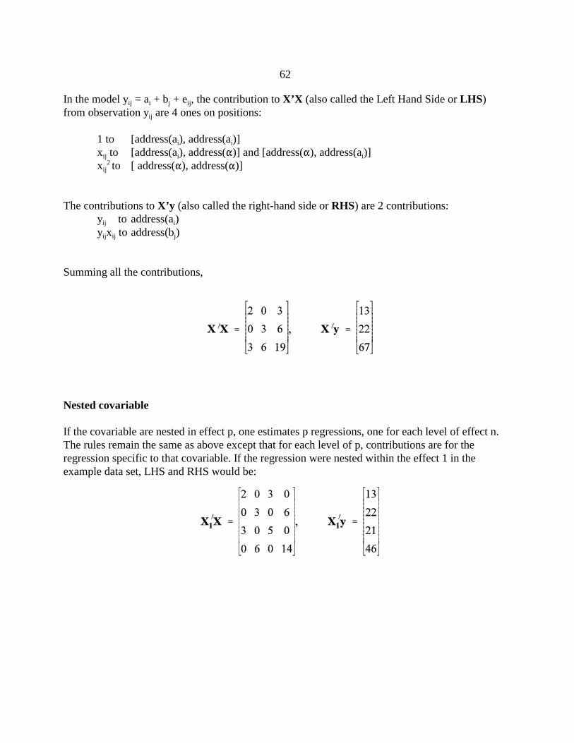
In the model yij = ai + bj + eij, the contribution to X’X (also called the Left Hand Side or LHS)from observation yij are 4 ones on positions:

[address(ai), address(ai)] [address(ai), address(bj)] [address(bj), address(ai)] [address(bj), address(bj)]

The contributions to X’y (also called the right-hand side or RHS) are 2 values of yij on positions:address(ai)address(bj)

56

If the number of levels were large, say in the thousands, the explicit calculation of X’X wouldinvolve billions of arithmetic operations, mostly on zeros. By calculating only nonzero entries ofLHS and RHS, the number of operations is in the thousands.

Using the rules, calculate contributions to LHS and RHS from all five observations

i j Contributions to LHS Contributions to LHS

1 1 (1,1),(1,3),(3,1),(3,3) add 5 to element 1 and 3





Summing all the contributions,

Please note the diagonal and symmetrical structure for X’X.

Extension to more than two effects

For n effects, each observation will contribute n2 ones to the LHS and n values to the RHS.Proceed as follows:1. For each observation, calculate addresses: addressi, i=1,n for each of the effect2. Add 1 to LHS elements (addressi, addressj), i=1,n, j=1,n3. Add observation value to RHS, elements (addressi), i=1,n4. Continue for all observations.

57

Example

Assume a four-effect model with the following number of levels:

effect number of levels1 (a) 502 (b) 1003 (c) 404 (d) 10

Assume the following observation:a11, b67, c24, d5, y=200

The addresses will be calculated as:

effect starting address for this effect address1 0 0+11=112 50 50+67=1173 100+50=150 150+24=1744 50+100+40 190+5=195

1 would be added to the following LHS locations: (11,11), (11,117), (11,174), (11,195), (117,11),(117,117),117,174),117,195), (174,11), (174,117), (174,174), (174,195), (195,11), (195,117),(195,174), (195,195)

200 will be added to the following RHS locations: 11, 117, 174 and 195.

58

Computer program

program lsqimplicit none!!This program calculates least square solutions for a model with 2 effects. !All the storage is dense, and solutions are obtained iteratively by!Gauss-Seidel. ! This model is easily upgradable to any number of effects!real, allocatable:: xx(:,:),xy(:),sol(:) !storage for the equationsinteger, allocatable:: indata(:) !storage for one line of datainteger,parameter:: neff=2,nlev(2)=(/2,3/) !number of effects and levelsreal :: y ! observation valueinteger :: neq,io,i,j ! number of equations and io-statusinteger,allocatable::address(:) !neq=sum(nlev)allocate (xx(neq,neq), xy(neq), sol(neq),indata(neff),address(neff))xx=0; xy=0!open(1,file='data_pr1')! do read(1,*,iostat=io)indata,y if (io.ne.0) exit call find_addresses do i=1,neff do j=1,neff xx(address(i),address(j))=xx(address(i),address(j))+1 enddo xy(address(i))=xy(address(i))+y enddoenddo!print*,'left hand side'do i=1,neq print '(100f5.1)',xx(i,:)enddo!print '( '' right hand side:'' ,100f6.1)',xy!call solve_dense_gs(neq,xx,xy,sol) !solution by Gauss-Seidelprint '( '' solution:'' ,100f7.3)',sol contains subroutine find_addresses integer :: i do i=1,neff address(i)=sum(nlev(1:i-1))+indata(i) enddo end subroutine

59

end program lsq

subroutine solve_dense_gs(n,lhs,rhs,sol)! finds sol in the system of linear equations: lhs*sol=rhs! the solution is iterative by Gauss-Seidelinteger :: nreal :: lhs(n,n),rhs(n),sol(n),epsinteger :: round!round=0do eps=0; round=round+1 do i=1,n solnew=sol(i)+(rhs(i)-sum(lhs(i,:)*sol))/lhs(i,i) eps=eps+ (sol(i)-solnew)**2 sol(i)=solnew end do if (eps.lt. 1e-10) exitend doprint*,'solutions computed in ',round,' rounds of iteration'end subroutine

60

Model with covariables

Datai xj yij1 1 51 2 82 1 72 2 62 3 9

Write the model as yij = ai + "xj + eij, where " is coefficient of regression.


For the first two observations:

61

For a two-factor model with covariables, the contribution to X’X from one observation is always4 elements in a square, with values being one, the value of then covariable or its square.

The contribution to X’y from one observation is always two elements with the values of thecurrent observation possibly multiplied by the value of the covariable.

Rules

Define a function address(effect) that defines the solution number corresponding to i-th effectand j-th level

Effect Address(effect)

a1 1

a2 2

" 3

62

In the model yij = ai + bj + eij, the contribution to X’X (also called the Left Hand Side or LHS)from observation yij are 4 ones on positions:

1 to [address(ai), address(ai)]xij to [address(ai), address(")] and [address("), address(ai)]xij

2 to [ address("), address(")]

The contributions to X’y (also called the right-hand side or RHS) are 2 contributions:yij to address(ai)yijxij to address(bj)

Summing all the contributions,

Nested covariable

If the covariable are nested in effect p, one estimates p regressions, one for each level of effect n.The rules remain the same as above except that for each level of p, contributions are for theregression specific to that covariable. If the regression were nested within the effect 1 in theexample data set, LHS and RHS would be:

63

Computer program Changes relative to the previous program are highlighted.

program lsqrimplicit none!! As lsq but with support for regular and nested regressions!integer,parameter::effcross=0,& !effects can be cross-classified effcov=1 !or covariablesreal, allocatable:: xx(:,:),xy(:),sol(:) !storage for the equationsinteger, allocatable:: indata(:) !storage for one line of effectsinteger,parameter:: neff=2,nlev(2)=(/2,3/) !number of effects and levelsinteger :: effecttype(neff)=(/effcross, effcov/) integer :: nestedcov(neff) =(/0,1/)real :: weight_cov(neff) real :: y ! observation valueinteger :: neq,io,i,j ! number of equations and io-statusinteger,allocatable::address(:) !neq=sum(nlev)allocate (xx(neq,neq), xy(neq), sol(neq),indata(neff),address(neff))xx=0; xy=0!open(1,file='data_pr1')! do read(1,*,iostat=io)indata,y if (io.ne.0) exit call find_addresses do i=1,neff do j=1,neff xx(address(i),address(j))=xx(address(i),address(j))+& weight_cov(i)*weight_cov(j) enddo xy(address(i))=xy(address(i))+y *weight_cov(i) enddoenddo!print*,'left hand side'do i=1,neq print '(100f5.1)',xx(i,:)enddo!print '( '' right hand side:'' ,100f6.1)',xy!call solve_dense_gs(neq,xx,xy,sol) !solution by Gauss-Seidelprint '( '' solution:'' ,100f7.3)',sol contains

64

subroutine find_addresses integer :: i do i=1,neff select case (effecttype(i)) case (effcross) address(i)=sum(nlev(1:i-1))+indata(i) weight_cov(i)=1.0 case (effcov) weight_cov(i)=indata(i) if (nestedcov(i) == 0) then address(i)=sum(nlev(1:i-1))+1 elseif (nestedcov(i)>0 .and. nestedcov(i).lt.neff) then address(i)=sum(nlev(1:i-1))+indata(nestedcov(i)) else print*,'wrong description of nested covariable' stop endif case default print*,'unimplemented effect ',i stop end select enddo end subroutine end program lsqr subroutine solve_dense_gs(n,lhs,rhs,sol)! finds sol in the system of linear equations: lhs*sol=rhs! the solution is iterative by Gauss-Seidelinteger :: nreal :: lhs(n,n),rhs(n),sol(n),epsinteger :: round!round=0do eps=0; round=round+1 do i=1,n if (lhs(i,i).eq.0) cycle solnew=sol(i)+(rhs(i)-sum(lhs(i,:)*sol))/lhs(i,i) eps=eps+ (sol(i)-solnew)**2 sol(i)=solnew end do if (eps.lt. 1e-10) exitend doprint*,'solutions computed in ',round,' rounds of iteration'end subroutine

65

Multiple trait least squares

Asume initially that the same model applies to all traits and that all traits are recorded. Thegeneral model is the same:

y = X$ + e, but V(y)=V(e) = R = R0qI

and can be decomposed into t single-trait equations with correlated residuals:

y1 = X1$1 + e1y2 = X2$2 + e2......................yt = Xt$t + et

where t is the number of traits, and V(y)=V(e)=R

and the normal equations are XR-1X $ = XR-1y

The detailed equations will depend on whether the equations are ordered by effects within traits orby traits within effects. In the first case, assuming all design matrices are equal

X0 = X1 = X2 = ...= Xt

and all traits are recorded, then:

and

where R0 is a t x t matrix of residual covariances between the traits in one observation.

66

Using the direct product notation that

this system of equations could be presented as:

where as if the equations were ordered by traits within effects,

Please note that $’s in both examples are not ordered the same way.

In the last case, the rules for creating normal equations are similar to those for single-trait modelsexcept that :

LHS: Instead of adding 1, add R-0

1

RHS: Instead of adding a scalar yi, add R-0

1 yi, where yi is a tx1 vector of data forobservation i.

Example

Assume the same data as before but with two traitsDatai j y1ij y2ij1 1 5 21 2 8 42 1 7 32 2 6 5 2 3 9 1

and assume that the correlations between the traits are

67


y = ( X1 + X2 + X3 + ... ) $ + e

Observation: first second third For the first two observations:

68

The bold zeros in the last matrix are in fact 2x2 matrices of zeros.

The bold zeros are 2x1 vectors of zeros.

Rules

Let address(effect,trait) be a function returning the addresses of level

! repeat these loops for each observation!do e1=1,neffect do e2=1,neffect do t1=1,ntrait

69

do t2=1,ntrait i=address(e1,t1)

j=address(e2,t2) XXi,j=XXi,j+rt1,t2

enddo t2 enddo t1 enddo e2enddo e1

do e1=1,neffect do t1=1,ntrait do t2=1,ntrait i=address(e1,t1)

XYi=XYi + rt1,t2 * yt2 enddo t1 enddo e2enddo e1

Missing traits

If some traits are missing, the general rules apply but R-0

1 is replaced by Rm, a matrix specific foreach missing-trait pattern m. Let Qm be a diagonal matrix that selects which traits are present. For

example, this matrix selects traits 1, 3 and 4. If some traits are missing, for each pattern ofmissing traits m, replace

R-01 by Rm = (Qm Ro Qm)-1

Qm Ro Qm can be created by zeroing rows and columns of Ro corresponding to missing traits.

Because then contributions due to missing equations to LHS and RHS are always zero, acomputer program may be made more efficient by modifications so that the zero contributions arenever added. Also, Rm’s can be precomputed for all combinations of missing traits. This isimportant if the number of traits is large.

70

Different models per trait

There are two ways of supporting such models:

1. By building the equations within models.This is the most flexible way but does not allow for easy utilization of blocks for sameeffects within traits. Makes iterative methods to solve MME (mixed model equations)slow.

2. By building the equations within traits, i.e., declaring same model for each trait and thenselectively nulling unused equations

This is more artificial way but results in simpler programs and possible more efficientCPU-wise (but not memory-wise).

Example of ordering by models and by traits

Assume the following models for the three beef traits:

Birth weight = cg + " age_dam + an + mat +e (150) (1) (1000) (1000)Weaning weight = cg + an + mat +e (100) (1000) (1000)Yearling weight = cg + an +e (50) (1000)

where " is a coefficient of regression on age of dam and cg is contemporary group, an is animaldirect and mat is animal maternal, and number of levels are in () .

Let xi,j be the j-th level of i-th trait of effect x. The order of the equations would be as follows:

Ordering withintraits

Ordering within models

71

cg1,1cg2,1cg3,1...cg1,150cg2,150cg3,150 "1"2"3 an1,1an2,1an3,1...an1,1000an2,1000an3,1000mat1,1mat2,1mat3,1...mat1,1000mat2,1000mat3,1000

cg1,1cg1,2...cg1,150"an1,1an1,2...an1,1000 mat1,1mat1,2...mat,1000 cg2,1cg2,2...cg2,100an2,1an2,2...an2,1000 mat1,1mat1,2...mat,1000cg3,1cg3,2...cg3,50an3,1an3,2...an3,1000

Please note that with ordering within models, only existing effects are defined. With orderingwithin effects, for regularity all 3 traits have 150 levels of cg and all have the maternal effectdefined.

72

Computer program

This program supports multiple-trait least squares with support for missing traits and missingeffects. Lines changed from the previous program are highlighted.

program lsqmtimplicit none!! As lsqr but with support for multiple traits!integer,parameter::effcross=0,& !effects can be cross-classified effcov=1 !or covariablesreal, allocatable:: xx(:,:),xy(:),sol(:) !storage for the equationsinteger, allocatable:: indata(:) !storage for one line of effects integer,parameter:: neff=2,& !number of effects nlev(2)=(/2,3/),& !number of levels ntrait=2,& !number of traits miss=0 !value of missing trait/effectreal :: r(ntrait,ntrait)=& !residual covariance matrix reshape((/1,2,2,5/),(/2,2/)),& ! values 1, 2 ,2 and 5 rinv(ntrait,ntrait) ! and its inverseinteger :: effecttype(neff)=(/effcross, effcov/)integer :: nestedcov(neff) =(/0,0/)real :: weight_cov(neff,ntrait) real :: y(ntrait) ! observation valueinteger :: neq,io,i,j,k,l ! number of equations and io-statusinteger,allocatable:: address(:,:) ! start and address of each effect !neq=ntrait*sum(nlev)allocate (xx(neq,neq), xy(neq), sol(neq),indata(neff*ntrait),& address(neff,ntrait))xx=0; xy=0!open(1,file='data_pr3')! do read(1,*,iostat=io)indata,y if (io.ne.0) exit call find_addresses call find_rinv do i=1,neff do j=1,neff do k=1,ntrait do l=1,ntrait xx(address(i,k),address(j,l))=xx(address(i,k),address(j,l))+& weight_cov(i,k)*weight_cov(j,l)*rinv(k,l) enddo enddo enddo do k=1,ntrait

73

do l=1,ntrait xy(address(i,k))=xy(address(i,k))+rinv(k,l)*y(l)*weight_cov(i,k) enddo enddo enddoenddo!print*,'left hand side'do i=1,neq print '(100f5.1)',xx(i,:)enddo!print '( '' right hand side:'' ,100f6.1)',xy!call solve_dense_gs(neq,xx,xy,sol) !solution by Gauss-Seidelprint '( '' solution:'' ,100f7.3)',sol contains subroutine find_addresses integer :: i,j,baseaddr do i=1,neff do j=1,ntrait if (datum(i,j) == miss) then !missing effect address(i,j)=0 !dummy address weight_cov(i,j)=0.0 cycle endif baseaddr=sum(nlev(1:i-1))*ntrait+j !base address (start) select case (effecttype(i)) case (effcross) address(i,j)=baseaddr+(datum(i,j)-1)*ntrait weight_cov(i,j)=1.0 case (effcov) weight_cov(i,j)=datum(i,j) if (nestedcov(i) == 0) then address(i,j)=baseaddr elseif (nestedcov(i)>0 .and. nestedcov(i).lt.neff) then address(i,j)=baseaddr+(datum(nestedcov(i),j)-1)*ntrait else print*,'wrong description of nested covariable' stop endif case default print*,'unimplemented effect ',i stop end select enddo enddo end subroutine function datum(ef,tr) real::datum integer :: ef,tr ! calculates the value effect ef and trait tr

74

datum=indata(ef +(tr-1)*neff) end function subroutine find_rinv! calculates inv(Q R Q), where Q is an identity matrix zeroed for ! elements corresponding to y(i)=miss integer :: i,irank real:: w(10) rinv=r do i=1,neff if (y(i) == miss) then rinv(i,:)=0; rinv(:,i)=0 endif enddo call ginv(rinv,ntrait,1e-5,irank) end subroutine end program lsqmt subroutine solve_dense_gs(n,lhs,rhs,sol)! finds sol in the system of linear equations: lhs*sol=rhs! the solution is iterative by Gauss-Seidelinteger :: nreal :: lhs(n,n),rhs(n),sol(n),epsinteger :: round!round=0do eps=0; round=round+1 do i=1,n if (lhs(i,i).eq.0) cycle solnew=sol(i)+(rhs(i)-sum(lhs(i,:)*sol))/lhs(i,i) eps=eps+ (sol(i)-solnew)**2 sol(i)=solnew end do if (eps.lt. 1e-10) exitend doprint*,'solutions computed in ',round,' rounds of iteration'end subroutine

Below is a generalized-inverse subroutine that needs to be compiled with the previous program.

subroutine ginv(a,n,tol,rank)! returns generalized inverse of x(n,n). tol is working zero ! and irank returns the rank of the matrix. rework of rohan fernando's ! f77 subroutine by i. misztal 05/05/87-05/23/00

implicit none integer n real a(n,n),w(n),tol,rank integer i,ii,j rank=n

75

do i=1,n do j=1,i-1 a(i:n,i)=a(i:n,i)-a(i,j)*a(i:n,j) enddo if (a(i,i).lt.tol) then a(i:n,i)=0.0 rank=rank-1 else a(i,i)=sqrt(a(i,i)) a(i+1:n,i)=a(i+1:n,i)/a(i,i) endif enddo

do i=1,n if (a(i,i).eq.0.) then a(i+1:n,i)=0 else a(i,i)=1.0/ a(i,i) w(i+1:n)=0 do ii=i+1,n w(ii:n)=w(ii:n)-a(ii:n,ii-1)*a(ii-1,i) if (a(ii,ii).eq.0.) then a(ii,i)=0. else a(ii,i)=w(ii)/a(ii,ii) endif enddo endif enddo

do j=1,n do i=j,n a(i,j)=dot_product(a(i:n,j),a(i:n,i)) enddo enddo

do i=1,n a(i,i+1:n)=a(i+1:n,i) enddo end

76

Mixed models

The traditional notation y = X$ + Zu +e, E(y)= X$, V(y)=ZGZ’ +R, V(u)=G, V(e)=Rgives little detail on differences betwen least squares and mixed models. The mixed modelequations (MME) are:

and sometimes are presented as

The only difference between mixed and fixed model equations is the inclusion of G-1. OtherwiseW’s are created the same way as X before. The main problem in mixed model equations isfiguring out what G-1 is and how to create it. Usually, G-1 can be decomposed into contributions from each effect or a combination of a feweffects. For example, let the random effects be u = [p, a, m, h]’, where p is permanentenvironment, a is animal direct, m is animal maternal, and h is herd by sire interaction. Then:

and contributions to G-1 can be calculated for each individual effect or groups of effectsseparately.

Popular contributions to random effects - single trait

1. Effects are identically and independently distributed (IID)Gi= IF2

i , where F2i is variance component for trait i. Then G-

i1 = I 1/F2

i . In this case, scalars1/F2

i are added to each diagonal element of LHS corresponding to effect i.

Popular IID effects are permanent environment and sire effect if relationships among siresare ignored.

77

2. Numerator relationship matrices- animal additive effect

Gi= AF2i , G-

i1 = A-1 1/F2

i

- sire additive effectGi= AsF

2i , G-

i1 = As

-1 1/F2i

- nonadditive genetic effects

3. Autoregressive structure matrixWhen adjacent levels of a random effect are correlated to the same degree, that effect mayhave an autoregressive structure (Wade and Quaas, 1993):

Gi= HF2i , G-

i1 = H-1 1/F2

iThis structure is useful for smoothing trends, e.g., in genetic groups, or accounting forcorrelations among observations in adjacent management levels.

4. Nonadditive effects. Formulas are available to obtain the inverse of the dominance (VanRaden and Hoeschele,1991) and additive x additive (Hoeschele and VanRaden, 1991) relationship matrices.

5. IBD

Distributions involving the I and A matrices are most popular.

Numerator relationship matrix A

For each individual i with sire s and dam d, the following recursive equation applies

ai = ½(as + ad) + mi

where mi is mendelian sampling and var(mi)=½ F2a(1-F)

If only parent p is known: ai = ½ap + mi, var(mi)=¾ F2a

If neither parent is known: ai = mi, var(mi)= F2a

In a connected population, the matrix A has all elements different from 0, and it is impossible tocreate directly. For example, A with 1,000,000 elements would have approximately 1012 nonzeroelements, too many to store anywhere. Fortunately Henderson (1985) has found that A-1 has veryfew nonzeros (at most 9 times the number of animals) and that it can easily be created. For all animalsa= P a + mwhere P is a matrix containing ½ and 0 that relates animals and parents, and m is the diagonal

78

matrix containing ½F2a, ¾ F2

a and F2a dependent on how many parents are known.

(I-P) a = m, a = (I-P)-1 m,

var(a) = A F2a =(I-P)-1 Var(m) [(I-P)-1]’

and A-1 = F2

a (I-P)’ Var(m)-1 (I-P)The only matrix left to invert is a diagonal matrix Var(m)

Rules to create A-1 directly

or the whole A-1 can be calculated from separate contribution from each animal in the pedigree.Let address(ai) point to the equation number of animal i, , address(as) and address(ad) to equationnumbers of sire and dam of animal i if present, and address(ap) point to equation number of parentp if the other parent is unknown. The contributions to A-1 from each animal would be

Please note that these contributions are results of (I-P) Var(m)-1 (I-P)’ for one animal:

where the coefficient 2 comes from var(mi)-1 = (½F2a)-1 = 2/F2

a.

79

When only one parent is known, the contributions are:

Finally, for animals with no parent known, the contribution is:

The contributions are done for each and every animal in the pedigree. For example, if one animalis present in the pedigree as a parent only, a separate equation should be created for this animaland a contribution to it added. Question: explain why the largest contributions are 2, 4/3 and 1!

Unknown parent groups

ai = ½(as + ad) + mi

If one or two parents are unknown, the merit for the unknown parent is assumed to be 0 and equalfor all unknown animals, regardless in what year their progeny was born, sex and origin of genes(domestic or international). Let’s assume that the genetic merit of unknown parent p is gp, and thatnow the animal effect accounts for unequal merit of unknown parents. Now:

ui = ½(us + ud) + mi, var(mi)=½ F2a(1-Fs/2 - Fd/2 )

where F are coefficients of inbreeding.

If only parent p1 is known: ui = ½(up1 + gp2) + mi, var(mi)=¾ F2a

If neither parent is known: ui = ½(gp1 + gp2) + mi, var(mi)= F2a

80

The contributions with the unknown parent groups are simpler than without the groups:

where k=2/ (4- number of known parents)

Groups have equations in the animal effect but are not treated as animals, i.e., they have noparents and 1 is not added to their diagonal as for animals without known parents.

Numerator relationship matrix in the sire model

The derivations below assume the absence of inbreeding, which cannot be calculated accurately inthe sire model.

For each bull i with sire s and maternal grandsire (MGS) t, the following recursive equationapplies

1) If sire and MGS known: si = ½(ss + ½sd) + mi, var(mi)=11/16F2s

2) If only sire s is known: si = ½ss + mi, var(mi)=¾ F2s

3) If only MGS is known: si = ¼sd + mi, , var(mi)=15/16 F2s

4) If neither parent is known: si = mi, var(mi)= F2s

The contributions to As-1 are done as for A-1 except that the values are:

These ratios are the result of multiplication of

81

where k is 16/11, 4/3, 16/15 and 1 for cases 1-4, respectively.

Autoregression

For t generated by a first-order autoregressive process:

with

where -1<D<1 is coefficient of autocorrelation and ,k is error term. Similar to the additive effects,the recurrence equations can be established as:

t =Pt + ,

where P is a matrix containing 1 and 0 that relate subsequent levels of t. Then:

(I-P) t = ,, t = (I-P)-1 ,,

var(t) = HF2t =[(I-P)-1]’ Var(,) (I-P)-1

and H-1 = F2

t (I-P)’ Var(,)-1 (I-P)

The only matrix left to invert is a diagonal matrix Var(,). While the matrix H has all nonzeroelements:

82

where n is the number of levels in t, its inverse has a tridiagonal structure:

The autocorrelation structure has been used to smooth effects such as unknown parent groups oryear-months within each herd. In the case of year months, there may be observations only in veryfew year-months. Then, the matrix H-1 = { hij} can be constructed in such a way so that allunneeded levels are skipped, by using the following rules:

where:

and dk is the distance between levels k and k+1.

Variance ratios

In single trait MME, the residual variance can be factored out from the equations:

83

= =

= =

If in the original MME, components of G-i1 had the form of

1/F2i I or 1/F2

i A

after the premultiplication, they will have the form ofF2

e/F2i I = ki I or F2

e/F2i A = ki A

where ki are variance ratios. Thus only variance ratios are necessary to set up the MME and notthe absolute variances.

Examples of calculation of the variance ratios

Assume that there is only one random effect in the model, either the sire effect or the animaleffect. Let us calculate the variance ratios given the heritability h2.

animal model

sire model

For h2 = .25, ka=3 and ks=13.

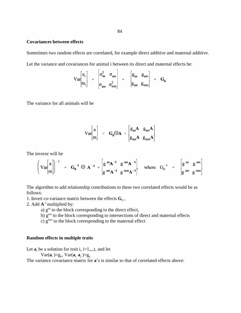
84

Covariances between effects

Sometimes two random effects are correlated, for example direct additive and maternal additive.

Let the variance and covariances for animal i between its direct and maternal effects be:

The variance for all animals will be

The inverse will be

The algorithm to add relationship contributions to these two correlated effects would be asfollows:1. Invert co-variance matrix between the effects G0 ,2. Add A-1 multiplied by:

a) gaa to the block corresponding to the direct effect,b) gam to the block corresponding to intersections of direct and maternal effectsc) gmm to the block corresponding to the maternal effect

Random effects in multiple traits

Let ai be a solution for trait i, i=1,,.,t, and letVar(ai )=gii, Var(ai, aj )=gij

The variance covariance matrix for a’s is similar to that of correlated effects above:

85

(54)

The inverse will be

The algorithm to add distribution contributions to correlated traits would be similar to that forcorrelated effects:1. Invert co-variance matrix between the traits G0 ,2. Add A-1 multiplied by:

a) gii to the block corresponding to trait i,b) gij to the blocks on intersections of traits i and j.

Multiple traits and correlated effects

For simplicity, assume only two traits: 1 and 2, and two effects: a and b.

Let ai,j be a vector of random effect i, i=a,b,... and trait j=1,2,.... Assume that all effects have thesame number of levels, var(ai,j)=gij,ijA, andvar(ai,j, akl)=gij,klA

The variance covariance matrix for a’s is similar to that of correlated effects above:

86

The remaining steps are similar as in the previous two sections.

Please note that for t traits and f correlated efects, the size of G0 will be tf x tf. For example fort=4 and f=2, the dimension will be 8 x 8 or 36 variance components.

87

Computer pseudo-codeLet add(i,j,k) be address of an equation of i-th effect, j-th level and k-th trait

Let aij be the value of A-1 for the i row and j-th column.Let gijkl be the value of G-

01 corresponding to i-k effect and j-k trait.

The following code would create corresponding contributions to the LHS of the MME.

do t1=1,ntrait do t2=1,ntrait do e1=”correlated effects” do e2=”correlated effects” LHS(block t1,t2,e1,e2) = LHS(block t1,t2,e1,e2) + A-1 *ge1,t1,e2,t2

enddo enddo enddoenddo

Below is a more detailed program for adding the animal relationship matrix. “Number ofcorrelated effects” will be 1 for effects uncorrelated with other effects, 2 if the currently processedeffect is correlated with the next one, etc.

real, parameter::w=(/1, -.5, -.5/) !matrix generating contributions to A-1

...........................do read animal, sire, dam and npar !npar=number of parents known if end of file then quit loop p(1)=animal; p(2)=sire; p(3)=dam do i=0,number of correlated effects - 1 do j=0,number of correlated effects - 1 do t1=1,ntrait do t2=1,ntrait do k=1,3 do l=1,3 m=address(effect+i,t1,p(k)) n=address(effect+j,t2,p(l)) xx(m,n)=xx(m,n)+g(effect+j,t1,effect+k,t2)* w(k)*w(l)*4./(4.-npar) enddo ............................ enddo

88

Computer program

Program LSQMT was modified to Program BLUP by including contributions for random effects.The following conventions apply:

- g(i,:,:) contains variances for effect i

- randomtype(i) contains types of random effects, as shown below

- randomnumb(i) shows how many successive random effects are correlated. For example,if randomnumb(3)=2, then contributions will also be made to effect 4 and blocks of effects3 and 4. If randomnumb(i)=p>1, then g(i,:,:) should have a rank of p*ntrait; the ordering ofg(i,:,:) is then within traits and by effects.

program BLUP1

! As lsqmt but with support for random effects............................................! Types of random effectsinteger, parameter :: g_fixed=1,& ! fixed effect g_diag=2, & ! diagonal g_A=3, & ! additive animal g_As=4 ! additive sire integer :: randomtype(neff),& ! status of each effect, as above randomnumb(neff) ! number of consecutive correlated effectsreal :: g(neff,20,20)=0 ! The random (co)variance matrix for each trait ! maximum size is 20 of trait x corr. effect combinations

........................

........................ ! Assign random effects and G and R matricesrandomtype=(/g_fixed, g_A/) !types of random effectrandomnumb=(/0, 1/) !number of correlated effects per effectg(2,1,1)=2; g(2,1,2)=-1; g(2,2,1)=g(2,1,2); g(2,2,2)=1r(1,1)=1; r(1,2)=0; r(2,1)=0; r(2,2)=1

call setup_g ! invert G matricesopen(2,file='pedname') !pedigree fileopen(1,file='data_pr3') !data file!................................................ ! Random effects' contributionsdo i=1,neff select case (randomtype(i)) case (g_fixed) continue ! fixed effect, do nothing case (g_diag) call add_g_diag(i) case (g_A, g_As)

89

call add_g_add(randomtype(i),i) case default print*,'unimplemented random type',randomtype(i) endselectenddo................................................ function address1(e,l,t)! returns address for given level l of effect e and trait t integer :: e,l,t, address1 address1= sum(nlev(1:e-1))*ntrait+(l-1)*ntrait+t end function

........................

........................ subroutine setup_g! inverts g matrices real :: w(20) integer :: rank do i=1,neff if (randomnumb(i).ne.0) then call printmat('original G',g(i,:,:),20,randomnumb(i)*ntrait) call ginv(g(i,:,:),20,1e-5,rank) call printmat('inverted G',g(i,:,:),20,randomnumb(i)*ntrait) endif enddo end subroutine

subroutine add_g_diag(eff)! adds diagonal (IID) contributions to MME integer :: eff, i,j,k,l,m,t1,t2 do i=1,nlev(eff) do j=0,randomnumb(eff)-1 do k=0,randomnumb(eff)-1 do t1=1,ntrait do t2=1,ntrait m=address1(eff+j,i,t1); l=address1(eff+k,i,t2) xx(m,l)=xx(m,l)+g(eff,t1+j*ntrait,t2+k*ntrait) enddo enddo enddo enddo enddo end subroutine subroutine add_g_add(type,eff)! generates contributions for additive sire or animal effect integer :: type,eff,i,j,t1,t2,k,l,m,n,io,animal,sire,dam,par_stat,p(3) real ::w(3),res(4)! select case (type) case (g_A) w=(/1., -.5, -.5/) res=(/2., 4/3., 1., 0./) case (g_As)

90

w=(/1., -.5, -.25/) res=(/16/11., 4/3., 15/15., 1./) end select

do read(2,*,iostat=io) animal, sire, dam,par_stat !status of parents if (io /= 0) exit p(1)=animal p(2)=sire p(3)=dam print*,p do i=0,randomnumb(eff) - 1 do j=0,randomnumb(eff) - 1 do t1=1,ntrait do t2=1,ntrait do k=1,3 do l=1,3 if (p(k)/=0 .and.p(l)/=0) then m=address1(eff+i,p(k),t1) n=address1(eff+j,p(l),t2) xx(m,n)=xx(m,n)+g(eff,t1+i*ntrait,t2+j*ntrait)*& w(k)*w(l)*res(par_stat) endif enddo enddo enddo enddo enddo enddo enddo end subroutine

end program blup1..........................................

91

A new function address1 that returns an address of an equation for effect e, level l and trait tallowed for a large reduction of complexity of subroutine find_addresses although thefunctionality of that subroutine remained unchanged.

subroutine find_addresses integer :: i,j,baseaddr do i=1,neff do j=1,ntrait if (datum(i,j) == miss) then !missing effect address(i,j)=0 !dummy address weight_cov(i,j)=0.0 cycle endif select case (effecttype(i)) case (effcross) address(i,j)=address1(i,datum(i,j),j) weight_cov(i,j)=1.0 case (effcov) weight_cov(i,j)=datum(i,j) if (nestedcov(i) == 0) then address(i,j)=address1(i,1,j) elseif (nestedcov(i)>0 .and. nestedcov(i).lt.neff) then address(i,j)=address1(i,datum(nestedcov(i),j) else print*,'wrong description of nested covariable' stop endif case default print*,'unimplemented effect ',i stop end select enddo enddoend subroutine

function address1(e,l,t)! returns address for given level l of effect e and trait t integer :: e,l,t, address1 address1= sum(nlev(1:e-1))*ntrait+(l-1)*ntrait+t end function

92

Storing and Solving Mixed Model Equations

Let n be the number of mixed model equations. The straightforward way to store the mixed modelequations would be in a square matrix, and the straightforward way to solve them would be to useone of general methods such as Gaussian elimination or LU decomposition. These methods wouldcost:

memory . n2 of double precision (8 bytes) numbersarithmetic operations . n3

Assuming a large 800 Mbyte memory, the memory limit would be approached at n . 10,000.Computing the solutions would take arithmetic operations . 1012, or 11 hrs for a computer with aspeed of 25 MFLOPS (million of floating point operations per second). For every problem twotimes larger, the memory requirements would quadruple and the computer time demands wouldincrease 8 times!

Let count the number of nonzero elements in MME. Let the model has e effects, t traits, and letthe only random effects be additive animal direct and maternal. Let the number of records be r,and let the total number of animals including ancestors be a. The number of nonzero contributionsto the LHS of MME N would be:

N < (et)2r + 4*9 a t 2

Maximum number ofcontributions due to records

Maximum number ofcontributions due topedigrees

Thus the number of nonzero coefficients depends linearly on the number of animals and records.Assume that the number of records is equal to the number of animals:

r= aand the number of equations is a function of the number of animals, say

n=4atThen, the number of nonzero elements per one row of LHS would be:

N/n < (36+ e2)t2a/ (4at) = t (e2/4 + 9)

For e=5 and t=3, N/n < 45.75. Assuming that each nonzero number is stored as three numbers:(aij, i,j) or in 16 bytes assuming that aij is double precision, the 800 Mbyte computer can now storeover 1 million equations, an increase of 100 fold! Further storage optimizations can increase thatnumber of few times.

Efficient computation of solutions to MME involves storing only nonzeros and doing arithmeticoperations on nonzeros only.

93

Storage of sparse matrices

Low storage requirements for MME can be achieved in several ways:- Exploiting the symmetry by storing upper- or lower-diagonal elements only (savings . 50%)- Storing only nonzeros (savings in the thousands)- Coding of repetitive fragments of MME

The following storage structures are popular:1. Ordered or unordered triples: (aij, i, j)

For a sample matrix of

the lower-diagonal storage by triples could be stored in a 3-column real matrix or one real vectorand 2-column integer matrix.

Triples is the simplest form of storing sparse matrices. It is not the most memory efficient, andmatrix organization cannot be easily deduced.

2. IJA where i-indices would point to elements with new rows.

94

Please note that now rows must be ordered.

In large matrices, IJA storage reduces the amount of memory necessary to store the rowinformation to a negligible amount.

IJA is an efficient method with fast access to rows although searching for a particular columncould be time consuming. Insertion of new elements is not easy with IJA and therefore thisstorage would mainly be used as a final form of storage, after conversion from other formats.

3. Linked listsIn linked lists, the row pointer points to the first element of each row, and each element

points to the next element, or “null” if it is the last element

95

Linked list can be implemented by “pointers”, i.e., using real dynamic memory allocation, or byusing vectors as below

Element RowPointer

Column Value Nextelementpointer

1 1 1 101 5

2 2 2 102 3

3 4 3 40 0

4 3 103 0

5 3 20 6

6 2 30 0

Linked list is not as memory efficient as IJA but it allows for easy insertion of new elements.

4. Trees Trees allow for fast access to particular element but are more complicated. Each node of a treecontains three items:a) Data point

- index- data

96

b) link to smaller node (null if node absent)c) link to larger node (null if node absent)

Tree is a flexible structure where extra elements can easily be added or eliminated. Adisadvantage is memory overhead for pointers, and more complicated programming.

Summing MME

The loops to generate the MME create LHS elements unordered. At least 50% of all the elementsare repeated. Solving algorithms mostly require the repeated coefficients summed and then sortedby row. The simplest way to do it is by sorting and summing:- store all the unsummed and unordered coefficients on disk,- sort by row and column- sum repeated contributions and store them in a way convenient for obtaining the solutions.

The number of unsummed contributions can be a few times larger than the number of summedcoefficients. Sorting requires scratch space of 2-3 times larger than the sorted file. Therefore thisapproach may requires a large temporary disk space up to 10 times the final coefficient file. Alsoit can be slow because sorting of large files on disk is slow. Therefore this approach should beavoided if alternatives are available.

If LHS is created directly in memory in a sparse form, for each k-th contribution to row i andcolumn j cijk one needs a method to quickly search whether the storage for i-j was already created.If yes, that contribution is updated. If no, it is created. Therefore, fast searching algorithms arecritical to the efficiency of setting up the MME.

97

Searching algorithms

For simplicity, searching methods below would search for one element a out of n element vectorb.

1. Linear unsorted list

Algorithm: check each entry sequentially Average cost: n/2 searches

2. Linked list

Linked list as shown above is many unsorted lists. The cost would be as above, but the n would be smaller (the average number of nonzero columns)

3. Binary search

Done on a sorted vector. One divides each vector in half, and finds which half has the searchedelement. The division continues until the final half has only 1 element. The average cost is log2(n), but one cannot insert new elements easily.

4. Tree

Properties of the trees are like those of a sorted vector but with capability of insertion anddeletion.The best case cost (balanced tree) is log2(n). The worst case cost (completely unbalanced tree) isn/2. Trees have higher overhead.

5. Hash

There are many hash methods. The most popular one is presented here. Let hash(a) be a function that :

a) returns values being addresses to elements of vector bb) for similar arguments returns very different addresses

The hash method works in the following way:a) calculate hash(a)b) check if that location in vector b contains the searched item

- if yes, exit- if that location is empty, return that location with status “empty”- if that location contain another item, add p and return to b)

The average cost of hash search is 1/0, where 0 is fraction of already filled elements in b. The

98

cost is indepenedent of the number of elements. Hash allows for fast addition of elements but notfor deletions.

For a scalar argument, the hash function can have a form hash(a)=mod(a*", n)+1,

where " is a large prime number. In this function, a unit of change in a causes an " change inhash. For multidimensional a, " would be a vector of large primes.

99

Numerical methods to solve a linear system of equations

Let Ax=b be the system of n linear equations. This section will assume, wherever applicable, that A is LHS of MME and therefore symmetricand semipositive definite, i.e., all eigenvalues of A are nonnegative.

The methods can be partitioned into:

1. Finite, where exact solutions are obtained in finite stages- dense matrix- sparse matrix

2. Iterative, where each similar step improves the accuracy of all solutions

Gaussian elimination

In Gaussian elimination the number of equations is reduced one by one, until there is only oneleft. After solving this equation, the remaining solutions are calculated by backsolving. Gaussianelimination is non competitive with the other methods and is rarely utilized. In the past, it wasused to eliminate one (and sometimes two) effects with the most numerous levels (CG) so thatonly a handful of equations could be solved. Absorption was useful with the sire model when thenumber of sires was much lower than the number of contemporary groups and when memory waslimited but with the animal model the savings are limited and sometimes negative (because thenumber of nonzero coefficient can increase --see fill-in sparse methods). One specific applicationof Gaussian elimination was absorption, i.e., Gaussian elimination of one effect when setting upMME.

Assume a single trait model y = Hf + Wt + ewhere f is vector of a fixed crossclassified effect to be absorbed and t is vector of all the remainingeffects. The MME are:

Since

the equation after the absorption is:

100

The computations are as follows:a) sort the data by effect to be absorbed,b) read the data one level effect f at a time creating W’W, W’y, and accumulating:

d = (H’H)ii - number of observations in the current level iyt = (H’y)i - total for all observations in level i

hw = (H’W)i - vector of counts between fi and tc) subtract

(H’W)i’ yt/d from W’y(H’W)i’ (H’W)i/d from W’W

d) continue to b) until end of datae) add G-1 and solve

LU decomposition (Cholesky factorization)

Decompose A= LU, where L is lower and U is upper diagonal, and solve in 2 stages:LU x = b as Ly = b and Ux = ySolving triangular systems of equations is easy.

For symmetric matrices, L=U’ such that LL’=A is called the Cholesky factorization.

L is easy to derive from the recursive formulas.

101

The computations may be done by columns or by rows

!by columnsdo i=1,n

do j=i+1,n

end doend do

!by rowsdo i=1,n

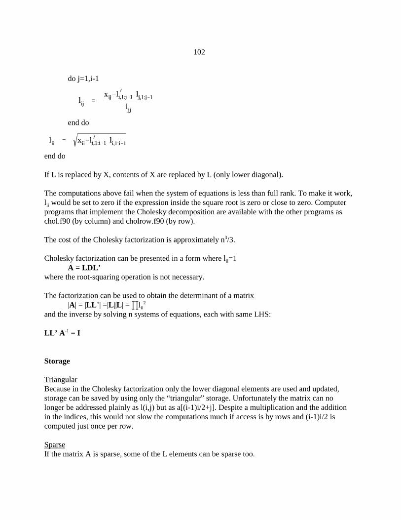
102

do j=1,i-1

end do

end do

If L is replaced by X, contents of X are replaced by L (only lower diagonal).

The computations above fail when the system of equations is less than full rank. To make it work,lii would be set to zero if the expression inside the square root is zero or close to zero. Computerprograms that implement the Cholesky decomposition are available with the other programs aschol.f90 (by column) and cholrow.f90 (by row).

The cost of the Cholesky factorization is approximately n3/3.

Cholesky factorization can be presented in a form where lii=1A = LDL’

where the root-squaring operation is not necessary.

The factorization can be used to obtain the determinant of a matrix|A| = |LL’| =|L||L| = Jlii

2

and the inverse by solving n systems of equations, each with same LHS:

LL’ A-1 = I

Storage

TriangularBecause in the Cholesky factorization only the lower diagonal elements are used and updated,storage can be saved by using only the “triangular” storage. Unfortunately the matrix can nolonger be addressed plainly as l(i,j) but as a[(i-1)i/2+j]. Despite a multiplication and the additionin the indices, this would not slow the computations much if access is by rows and (i-1)i/2 iscomputed just once per row. SparseIf the matrix A is sparse, some of the L elements can be sparse too.

103

TheoremIf a(i,j)#0 and a(i,k)#0 for j,k>i, then l(j,k)#0 even if a(j,k)#0

An element nonzero in L but not in A is called fill-in. To minimize the number of fill-ins,equations can be reordered.

Example

Calculate L for a random model for 5 sires, each with 2 observation; variance ratio = 2.

Model I yij=:+si+eijModel II yij=si+:+eij

The LHS denotes as A and the corresponding L are shown below

Both models resulted in LHS with the same number in zero. However, L in model 1 wascompletely filled because of many fill-ins, while L in model 2 had no fill-ins and remained sparse.

In sparse matrix factorization, the following steps are performed:a) Finding the ordering Q so that minimizes the number of fill-ins in QAQ’,b) Preparing storage structures for L

104

c) Computing the factorization LL’=QAQ’d) Solving the system QAQ’ Qx = Qb as LL’y =c and x=Q’b

Matrix Q is a permutation of the identity matrix. Thus it can be stored as a vector, and all vectormultiplications will involve a vector.

Steps a) and b) need to be done just once for each nonzero structure of A. If only values of Achange, only step c) and d) need to be repeated. If only RHS changes, only step d) need to berepeated.

cost(sparse L) -n [z(1+ f)]2 where z is the average number of nonzeroes per row, and f is the fraction of fill-ins. For animalmodel problems, sparse factorization allows to work with matrices about 10-50 times larger thanthe dense-matrix factorization.

Ordering is a complicated process. Excellent coverage of sparse methods is in books by Georgeand Liu (1981) and Duff et al. (1989). Packages for sparse matrix operations include commercialSPARSPAK, SMPAK, MA 28, or public domain FSPAK (anonymous ftp at num.ads.uga.edu,directory FSPAK).

Sparse matrix inversion

Even if the LHS is sparse, usually the inverse of the LHS is dense. Therefore, storage of such acomplete matrix would be impossible for dimensions over 10,000-20,000! (why?). For operationssuch as variance components by REML or accuracies (PEV), only selected animals of the inverseare required. If sparse factorization is available, one can obtain inverse elements corresponding tononzeros of the factorization at a cost of twice the factorization, using the Takahashi algorithm.Clarification: for the purpose of the inversion, nonzeros in L mean elements that were created butcould have values of zero due to numerical cancellation.

For the diagonal factorization: A= LDL’

A-1 = D-1L-1 + (I-L’)A-1

By starting the computations from the last row/column, it is possible to avoid the computations ofL-1 explicitly.

The drawing below shows the progress of computations of a sparse inverse. The computationrequires a access to L by columns or row access to L’. Please note that the computations start withthe last diagonals and progress up to the first row. The sparse inverse, as computed, replaces thefactorization without the need for much extra memory.

105

The operations on rows of sparse matrices require sparse vector by sparse vector multiplication.Since two sparse vectors generally need not share the same nonzero structure, the multiplication ishard to do directly. Therefore this is done in several stepsa) zero a work dense vector, b) uncompress the first sparse vector to the dense vectorc) multiply the second sparse vector by the dense vector (easy),d) zero elements of the dense vector changed in step b)

106

Example: define the sparse vector p as triple (pn pia pa) pn - size of vectorpia - vector of nonzero columnspa - vector of nonzero values

Let the work dense vector be w. This program would multiply x by y

! sum=x*y! uncompress xdo i=1,xn w(xia(i))=xa(i)enddo! w*ysum=0do i=1,yn sum=sum+w(yia(i))*ya(i)enddo! nullify changed elements of wdo i=1,xn w(xia(i))=0enddo

Numerical accuracy

Usually, dense matrix operations use double-precision numbers to avoid numerical inaccuracies.Errors usually propagate in finite methods, i.e., an error done during the computations of onematrix element is usually compounded during the computations of the following elements. Onecritical point in Cholesky factorization of matrices of not full rank is the detection of unnecessaryequations, which may be less than perfect. Making LHS full-rank by eliminating the unnecessaryrows explicitly solves the problem. Sparse factorization results in more accurate computationsbecause of fewer computations and therefore fewer rounding errors.

107

Iterative methods

In iterative methods, a sequence of solutions is produced

x0 , x1, x2,..., xi,

where each subsequent solution is more accurate than the previous one. The two simplestiterations are Jacobi and Gauss-Seidel. They originate from a family of stationary iterationmethods where iteration parameters stay constant during all rounds of iteration.Decompose A into a part that can easily be inverted M and the remainder N

A=M+N

and write

Ax=b,(M+N)x = b,Mx = -Nx +b

In the iteration:

Mx(n+1)=-Nx(n) +b

the iterative solution is obtained as

x(n+1)= M-1(-Nx(n) +b)

Let A be decomposed as

where for symmetric matrices U = L’

108

JacobiIn the Jacobi method, M=D, and N=L+U

x(n+1)= x(n) + D-1 (b - A x(n))where D=diag(A) is a diagonal matrix

or

do i=1,n

enddo In the Jacobi iteration, newly computed solutions are not used until all the new solutions areknown.

Gauss-Seidel and SOR

In Gauss Seidel the computations are similar to Jacobi but the newly computed solutions are usedimmediately

do i=1,m

enddo

The GS iteration can be rearranged to

Thus, this iteration is equivalent to obtaining (L+D)-1 which better approximates A-1 than D-1 inthe Jacobi iteration and therefore can be expected to have better properties.

The computer program for the Gauss-Seidel iteration is very easy, assuming that new solutions

109

immediately replace the old solutions

do i=1,n

enddo

or

do i=1,n diff=b(i)-matmul(a(i,:),x) x(i)=x(i)+diff/a(i,i)enddo

The successive overrelaxation (SOR) is modified GS

do i=1,n

enddo

where T is the relaxation factor. For complicated LHS, a good choice of T,(1,2) results in a betterconvergence rate.

GS can be implemented with half- upper-stored A at a cost of storing an adjusted right hand side.When solution i is computed, the right hand side for equations i+1,..., can be adjusted for thatsolution. The program (one round only) would be

c=bdo i=1,n diff=c(i)-matmul(a(i,:),x) x(i)=x(i)+diff/a(i,i) c(i+1:n)=c(i+1:n)-matmul(a(i,i+1:n), x(i+1:n)enddo

110

Preconditioned conjugate gradient

The method of preconditioned conjugate gradient (PCG), as used in ITPACK, Berger et al. (1989) and by Lidauer et al. (1999), converges much faster for complicated models than either Gauss-Seidel, SOR or Jacobi. Good overview of the theory of PCG is in Meurant (1999)

PCG has some similarities to the second-order Jacobi, which is:

x(n+1)= x(n) + "(x(n) -x(n-1)) + $ D-1 (b - A x(n))

PCG uses a similar formula except that " and $ are recomputed every round for orthogonal (b - Ax(n)), and D is replaced by M, which is now called the preconditioner. M may equal to diag(A) orany other approximation of A that is easily invertable.

The complete pseudo code for the PCG iteration is:

x=0 ; r=b-Ax; k=1do while (r’r “not sufficiently small”) z=M-1 r Jk-1=z’r if (k==1) then $=0; p=z else $=Jk-1/Jk-2; p=z+$ p endif w=Ap "=Jk-1 /(p’w) x=x+"p if (mod(k,100) /=0) then r=r-"w else r=b-Ax endif k=k+1enddo

Despite a seemingly complicated code, PCG is very easy to implement because the only compute-intensive operations are Ax or Ap. As presented, the PCG algorithm needs 7 variables, but two ofthem: b and z can be eliminated, for a total of 5. This algorithm lacks the self-correctingproperties of Gauss-Seidel, SOR or second-order Jacobi iterations, and may diverge with largedata sets if the variables are not in double precision.

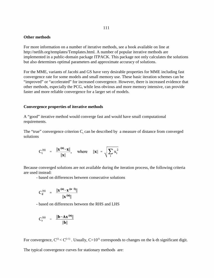
111

Other methods

For more information on a number of iterative methods, see a book available on line athttp://netlib.org/templates/Templates.html. A number of popular iterative methods areimplemented in a public-domain package ITPACK. This package not only calculates the solutionsbut also determines optimal parameters and approximate accuracy of solutions.

For the MME, variants of Jacobi and GS have very desirable properties for MME including fastconvergence rate for some models and small memory use. These basic iteration schemes can be“improved” or “accelerated” for increased convergence. However, there is increased evidence thatother methods, especially the PCG, while less obvious and more memory intensive, can providefaster and more reliable convergence for a larger set of models.

Convergence properties of iterative methods

A “good” iterative method would converge fast and would have small computationalrequirements.

The “true” convergence criterion Ct can be described by a measure of distance from convergedsolutions

Because converged solutions are not available during the iteration process, the following criteriaare used instead:

- based on differences between consecutive solutions

- based on differences between the RHS and LHS

For convergence, C(i) < C(i-1) . Usually, C=10-k corresponds to changes on the k-th significant digit.

The typical convergence curves for stationary methods are:

112

In a typical convergence curve, a seemingly rapid convergence is followed by a steady rate ofconvergence, finally changing into random fluctuations. The convergence criteria based ondifferences between the consecutive solution show much better convergence than the “true”criterion. However, both are parallel during the period of steady convergence. Let’s determine thenecessary conditions for convergence and calculate the convergence rate based on a particularmethod of iteration.

A typical curve for a solution is

113

Lte’s determine why solutions are converging so smooth in later rounds of iteration.

The stationary iteration can be presented in a form

x(n+1)= B x(n) + c

Decompose B into eigenvalues and eignevectors. For nonsymmetric B, these are complex

B = VE’,

where E is diagonal, eii are eigenvalues, and rows of V: vi are eigenvectors, which are orthogonaland normalized only for symmetric B

The successive stages of the iteration can be presented as:

x(1)= B x(0) + c x(2)= B x(1) + c =B (B x(0) + c) +c = B2x(0) +Bc + cx(3)= B x(2) + c =B (B2x(0) +Bc + c) +c = B3x(0) +B2c + Bc + c...x(n)=Bnx(0) +Bn-1c +..+ Bc + c

and, assuming that x(0) = 0x(n) - x(n-1) = Bn-1c

Because the product Bn is

VE V- VEV- ... VE V- = V En V-

114

therefore

Arrange VEV so that the absolute values of the eigenvalues are ordered in the descending order|e1| $ |e2| $ ... $ |em|

If we assume |e1|>|e2| then for sufficiently large n

andBnc . e1

n v1 v1'1'c = |e1|n fThen

x(n) = x(n-1) + Bn-1c = x(n-1) + |e1|n-1 f

The last expression shows for convergence |e1n+1| < |e1

n| Y |e1| < 1, or that the largest eigenvaluemust be smaller than one. It also shows that for large n the changes in the solutions will be predictable, where the samevector f is added with a coefficient becoming e1 times smaller every next round. That predictablechange is the reason for a relatively flat convergence curve for larger n. We can rewrite theformula for covergence criterion based on differences between the consecutive solutions

and

Thus, the slope of the convergence curve for larger n is constant and determined by the largesteigenvalue of the iteration matrix.

Since for large n the solutions increase predictably, one can approximate x(4). From

x(n) = x(n-1) + Bnc = x(n-1) + |e1|n-1 f

the formula for x(4) will be

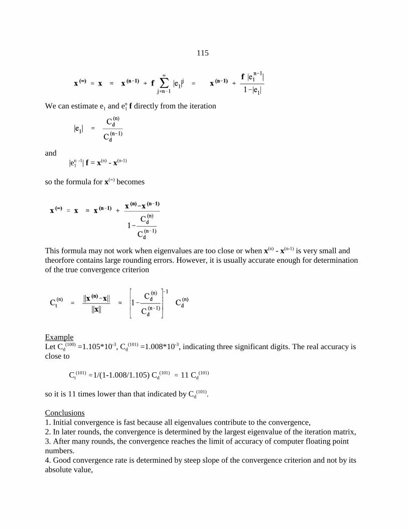
115

We can estimate e1 and e1n f directly from the iteration

and |e1

n -1| f = x(n) - x(n-1)

so the formula for x(4) becomes

This formula may not work when eigenvalues are too close or when x(n) - x(n-1) is very small andtheorfore contains large rounding errors. However, it is usually accurate enough for determinationof the true convergence criterion

ExampleLet Cd

(100) =1.105*10-3, Cd(101) =1.008*10-3, indicating three significant digits. The real accuracy is

close to

Ct(101) .1/(1-1.008/1.105) Cd

(101) . 11 Cd(101)

so it is 11 times lower than that indicated by Cd(101).

Conclusions1. Initial convergence is fast because all eigenvalues contribute to the convergence,2. In later rounds, the convergence is determined by the largest eigenvalue of the iteration matrix,3. After many rounds, the convergence reaches the limit of accuracy of computer floating pointnumbers.4. Good convergence rate is determined by steep slope of the convergence criterion and not by itsabsolute value,

116

5. The criterion based on differences in solutions between consecutive rounds of iteration cangrossly overstate the accuracy.

Properties of the Jacobi iteration

The Jacobi iteration leads to very simple programs because the expressionb-Ax

is easy to obtain for any format of A. In general, Jacobi converges for matrices diagonallydominant, where aii > aij, but usually the MME do not satisfy this condition. In practice, Jacobidiverges with more than one fixed effect and with animal-additive or dominance effect.

To converge with many fixed effects, the following modifications are generally successful:

- impose constrains on fixed effects, for example by forcing the sum of solutions for eachfixed effect except the first one to 0; the constrain by setting unnecessary equations to zeroresults in poor convergence, or

- update only one effect at a time

To converge with animal-additive or dominance effect, extend Jacobi to second-order Jacobi (alsocalled Chebyshev-accelerated)

x(n+1)= x(n) + "(x(n) -x(n-1)) + $ D-1 (b - A x(n))

where " and $ are iteration parameters, which are adjusted for the best convergence. In the animalmodel, the good parameters are "=.7-.9 and $=1. In the dominance model, additionally $ = .4-.6.

The Jacobi iteration is of interest only when the LHS is not available explicitly, as with iterationon data.

Properties of the Gauss-Seidel and SOR iterations

The GS and SOR iterations converge for all symmetric semipositive-definite matrices. Noconstrains are necessary for redundant equations or fixed effects. The disadvantage is thatelements of A must be available sequentially, row by row. As will be shown later, SOR hasadvantage over GS only for effects with nondiagonal blocks.

Practical convergence issues

117

Predictions of breeding values for genetic evaluation need to be calculated with very limitedprecision, no more than 2 decimal digits. Such precision is obtained with 5-15 rounds in a single-trait sire model, 30-100 rounds in a single-trait animal model. With models with multiple traitsand the maternal effect, the number of rounds can increase to > 500. One way of increasing theconvergence rate for multiple traits is to set the MME within traits and decompose

A = L + D + L’so that D would include diagonal blocks of traits, and possible blocks of direct and maternaleffects. Such a modification described by Dwyer and VanVleck (JDS, 1985?). Then, theconvergence rate with multiple traits is comparable to that with a single-trait.

Jacobi by effects, where only one effect is solved at a time, would be equivalent to a mixediteration where the outer iteration is GS and the inner iteration is Jacobi. Note that for fixedeffects where the diagonal blocks for effects are diagonal, Jacobi by effects is equivalent to Gauss-Seidel. A disadvantage of block iteration is increased storage for diagonal elements.

MME are usually not of full rank. While regular Jacobi iteration requires “sum to zero” for allfixed effects but one, Jacobi-by-effect, GS and SOR handle the MME well and do not need anyconstrains.

Determination of best iteration parametersSome iterations, including SOR and second order Jacobi, require the choice of quasi-optimaliteration parameters. Those parameters can be selected in a few ways, by 1. setting the iteration matrix B for several parameters, calculating eigenvalues, and selecting

parameters corresponding to the smallest e1; hard to do for large systems of equations 2. running the iteration many times with different parameters and selecting the parameter

with the best convergence rate in later rounds of iteration (lowest e1), 3. updating the parameters during the course of iteration, as in Hageman et al. (1981?) or

ITPACK.Usually parameters quasi-optimal for one data set remain quasi-optimal for similar data sets.

Strategies for iterative solutions

Solving by effects

Consider a model

where fi may be either random or fixed effect. The MME assuming for simplicity R=I are

118

This system of equation is equivalent to block equations

................................................................................

where yi(*) is vector of observations adjusted for all effects but i. Instead of solving the full MME

iteratively, it is possible to solve each block separately by any method, and repeat the solving byblocks until convergence.

Creating the adjusted observations is simple. For example, if a model for one observation is

5.2 = c1 + a20 + p15 + e

and if , the value of y adjusted for all effects except a would be

5.2 - 1.4 - 3.8 = 0.0

Iteration on data (matrix-free iteration)

If MME cannot be stored in memory but can be created on disk, the system of equations can besolved by repeatedly reading the MME from disk. However, reading from disk is relatively slow.The size of the LHS of MME can be 10 times or larger than the size of data, with differenceincreasing with the number of traits and effects. Therefore instead of reading the MME from diskit may be faster (and simpler) to read the much smaller data from disk and recreate necessary partsof MME each round.

Iteration on data (I.D.) is very simple when the iteration method involves A only in the expression

119

Ax(n)

This expression can be created as follows:

Original program I.D. program

...

A(i,j)=A(i,j)+z...

call solve(A,b,x)

...do round=1,p AX=0; D=0 ... ... if (i == j) D(i)=D(i)+z AX(i)=AX(i)+z*x(j) ... ... ! This is for Jacobi iteration only do i=1,neq x(i)=x(i)+(b(i)-AX(i))/D(i) end do end do.....

The statements to set-up D and AX are added for parts of the program corresponding tocontributions due to records and to contributions due to relationships.

When the iteration updates only one effect in one round, the modifications would be

do round=1,p AX=0; D=0 do e1=1,neff ... ... if (i == j) D(i)=D(i)+z AX(i)=AX(i)+z*x(j) ... ... ! This is for Jacobi iteration only do i=sum(nlev(1:e1-1)+1,i=sum(nlev(1:e1) x(i)=x(i)+(b(i)-AX(i))/d(i) enddo end do end do

120

Please see that the program statements related to relationship contributions are not shown aboveseparately. For the iteration that needs only the matrix-vector product Ax, the data and pedigreefiles need not be in any particular order. For multiple-trait block iteration, the programs would bemodified to create block-diagonal D.

The same strategy can be used in PCG except that the product to dervive can be either Ax or Ap.

The implementation of the Gauss-Seidel or SOR iteration is more difficult because LHS needs tobe available one row at a time. To do so: - for e effects, create e copies of the data file, each sorted for different effect - for pedigree file, create 3 copies, sorted by animal, sire and dam, respectively. - solve as follows:

do e=1,neff rewind i .....

..... do l=1,nlev(i) d=0 ax=0 current=address(e,l)

.....

..... do “read file sorted by level l until the end of level l”

.....

..... if (i == current) then if (i==j) d=d+z ax=ax+z*x(j)

endif end do !of reading the level l!

if (e is animal effect) thendo

read pedigree line with animal l &as either animal, sire or dam

....

....if (i == current) then

if (i==j) d=d+z ax=ax+z*x(j)

endif

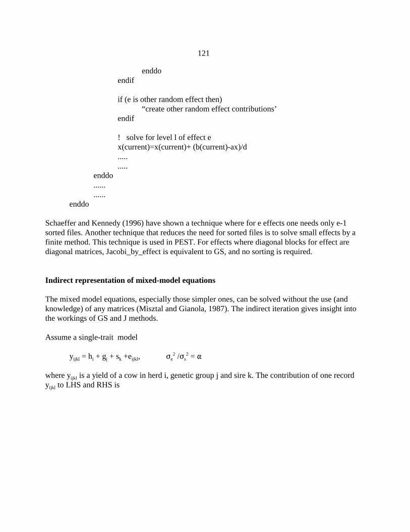
121

enddoendif

if (e is other random effect then)“create other random effect contributions’

endif

! solve for level l of effect e x(current)=x(current)+ (b(current)-ax)/d

.....

.....enddo............

enddo

Schaeffer and Kennedy (1996) have shown a technique where for e effects one needs only e-1sorted files. Another technique that reduces the need for sorted files is to solve small effects by afinite method. This technique is used in PEST. For effects where diagonal blocks for effect arediagonal matrices, Jacobi_by_effect is equivalent to GS, and no sorting is required.

Indirect representation of mixed-model equations

The mixed model equations, especially those simpler ones, can be solved without the use (andknowledge) of any matrices (Misztal and Gianola, 1987). The indirect iteration gives insight intothe workings of GS and J methods.

Assume a single-trait model

yijkl = hi + gj + sk +eijkl, Fe2 /Fs

2 = "

where yijkl is a yield of a cow in herd i, genetic group j and sire k. The contribution of one recordyijkl to LHS and RHS is

122

All the contributions corresponding to the row of hi result in an equation

The GS iteration for hi would be

or

The solution for hi is an average of observations that include hi adjusted for all the other effects.

Similarly, we can derive equations for gj and sk

123

The regression towards the mean in the last equation is due to sk being the random effect.

In the GS iteration, hi will be solved first, followed by gj and then by sk. In the Jacobi iteration, alleffects will be solved simultaneously.

Example

i j k yijkl

1 1 1 17

1 1 2 10

1 2 1 12

1 2 2 7

2 1 1 14

2 1 2 9

2 2 1 11

2 2 2 4

Assume that "=8 and that the initial solutions are 0. The first round solutions by GS are

h1 = (17+10+12+7)/4 = 11.5h2 = (14+9+11+4)/4=9.5g1 = [(17-11.5) + (10-11.5) + (14-9.5) + (9-9.5)]/4=2g2 = [(17-11.5) + (7-11.5) + (11-9.5) + ((4-9.5)]/4=-2

s1 = 4/(4+8) [ (17-11.5-2) + (12-11.5 -(-2)) + (14-9.5-2) + (11-9.5-(-2))]=1s2 = -1

The solutions will remain identical the next round so the convergence for this special balancedcase was reached in 1 round.

In Jacobi

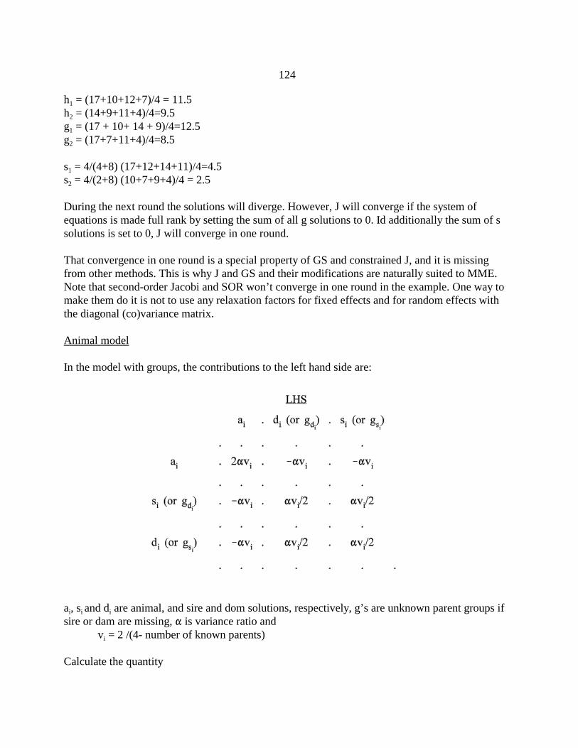
124

h1 = (17+10+12+7)/4 = 11.5h2 = (14+9+11+4)/4=9.5g1 = (17 + 10+ 14 + 9)/4=12.5g2 = (17+7+11+4)/4=8.5

s1 = 4/(4+8) (17+12+14+11)/4=4.5s2 = 4/(2+8) (10+7+9+4)/4 = 2.5

During the next round the solutions will diverge. However, J will converge if the system ofequations is made full rank by setting the sum of all g solutions to 0. Id additionally the sum of ssolutions is set to 0, J will converge in one round.

That convergence in one round is a special property of GS and constrained J, and it is missingfrom other methods. This is why J and GS and their modifications are naturally suited to MME.Note that second-order Jacobi and SOR won’t converge in one round in the example. One way tomake them do it is not to use any relaxation factors for fixed effects and for random effects withthe diagonal (co)variance matrix.

Animal model

In the model with groups, the contributions to the left hand side are:

ai, si and di are animal, and sire and dom solutions, respectively, g’s are unknown parent groups ifsire or dam are missing, " is variance ratio and

vi = 2 /(4- number of known parents)

Calculate the quantity

125

z = - " vi( 2 ai - di - si )The contribution to the adjusted right hand side (b-AX) from each pedigree line is:to animal

- " vi( 2 ai - di - si ) = zto sire (or sire unknown parent group)

" vi( 2 ai - di - si )/2 = -z/2to dam (or dam unknown parent group)

" vi( 2 ai - di - si )/2 = -z/2

The corresponding changes to the diagonal would be:to animal

2 " vito sire (or sire unknown parent group)

" vi /2to dam (or dam unknown parent group)

" vi /2

Example

Consider the “dairy” repeatability model

yijkl = mi + pj + ak + eijkl

where yijkl is yield of cows in management groups mi, with additive value ak and permanentenvironment pj, and

var(p)=IFp2, var(a)=AFa

2, Fe2/Fa

2=", Fe2/Fp

2=&

The matrix-free equations are

where prkl and matekl are the progeny and mate of the l-th mating of the k-th animal, respectively,

126

and vkl is the corresponding residual (=.5 if mate is known and 1/3 if mate is replaced by unknownparent group).

The extension of these rules to multiple traits, maternal effects etc. can be done following theabove methodology. For GS iteration, it was done by Kennedy and Schaeffer (1986, WCGALP).

Summary of iteration strategies

The GS and SOR iterations are the methods of choice when the coefficient matrix can be stored inmemory and simplicity is important. This would usually require memory of 100-1000bytes/equations. The iteration on data by modifications of Jacobi would be the next choice forsimpler models, with memory requirements of 12-16 bytes/equation. However, the method ofchoice nowadays seems to be PCG. Despite a seemingly complicated code, PCG is very easy toimplement because the only compute-intensive operations are Ax or Ap, especially with Fortran90 with vector instructions. PCG with diagonal preconditioner converged for all attemptedmodels, including multiple trait, random regressions, with maternal effect and dominance. Theconvergence rate was as good or better as J or SOR. Also, there are no acceleration parameters todetermine. One disadvantage of PCG is that it requires more memory: 36-56 bytes/ equations, butthis is not as much of a problem as it used to be.

127

Variance components

Out of very many methods for estimating variance components, three types are in popular usetoday (1998). They are:

1. REML2. Bayesian methods via Gibbs-sampling, also called Markov Chain Monte Carlo (MCMC),3. Method R.

REML is popular because of resistance to selection bias and the estimates are always within theparameter space. Its disadvantages include high cost for large models and relatively difficultprogramming especially for nonstandard models although various implementations of REMLdiffer widely in their computing properties.

Bayesian methods via Gibbs-sampling result in simple programs even for complicated models,and have good theoretical properties. Their disadvantage include slow convergence because ofthe Monte-Carlo origin and therefore very long running time for larger problems.

Method R is applicable to very large systems of equations and is simple to implement for commonmodels. However, the sampling error is higher than in the above methods, and incorrect fixedeffects can result in drastically biased estimates. Also, for multiple traits there are onlyapproximations.

REML

Let the model be y = X$ + e

where the distribution of y is multivariate normal with mean X$ and variance V,y ~ MVN(X$, V)

orVar(e) = V and E(y) =X$

Following Quaas (1990), the likelihood of $ and V is

where N is a vector or a matrix of variance components in V. This can be simplified to

128

The maximum likelihood (ML) estimates can be obtained by maximizing ln L. The ML estimatesof variance components depend on fixed effects because the degrees of freedom due to estimatingthe fixed effects are not taken into account. In restricted maximum likelihood, y is replaced by Mysuch that

MX= 0 Y My = Me

which is equivalent to integrating the fixed effects from the ML likelihood. In subsequentderivations M cancels out, and the log of the restricted maximum likelihood becomes

Most of the research in REML went into simplifying the above likelihood for particular modelsand into maximizing that likelihood. For mixed models, the log likelihood is proportional to

where C* is the coefficient matrix of the MME converted to full-rank; the determinant of asingular matrix is 0.

For

where Ri is the residual (co)variance matrix for observation i, and Gj is the (co)variance matrix forrandom effect j, the components of the likelihood can be further simplified to

In particular, for specific G’s,

where na and ni are the number of levels.

The REML estimates are derived by maximization

129

by one of the many maximization algorithms for nonlinear functions.

REML is relatively easy to evaluate. Matrices Ri and Gi0 are small. ln|C*| can be calculated fromthe Cholesky decomposition of LHS. Also, solutions can be obtained by Cholesky decomposition.

The simplest maximization is derivative-free:

a) choose a derivative-free maximization subroutine from a library (IMSL, “Numerical Recipes”,”www.netlib.org”,..)

b) write a function L(variance components) c) apply a) to b)

The computational constrain in derivative free methods would be time to calculate thedeterminant.

The alternate way to maximize the REML would be by using the first derivative,

which is a problem of finding zeroes of a multidimensional nonlinear function. In single traits,this leads to the following equations

where ni is the number of levels of random effect i, Fi2Ai is its (co)variance matrix, and Cii is a

diagonal block of the inverse of C corresponding to effect i. This formula can be deriveddifferently as EM REML. A faster converging version of the same formula is

where ni is the number of levels in the i-th random effect. The residual is estimated as

where nr is the number of records and r(X’X) is the rank of the fixed-effect part of the MME. Inthe first-derivative REML, the largest expense is in calculating the inverse of C. The trace can becomputed as

130

or as the sum of Ai-1 and Cii multiplied directly, element by element. When Ai

-1 is sparse, onedoes not require all elements of Cii but only those that are nonzero in Cii, or a small fraction of allinverse elements of C. The sparse inverse described before contains all the inverse elementsnonzero in Ai

-1. Computing that inverse from sparse factorization costs twice more thancomputing the factorization alone, and almost no extra memory. Thus, the most compute-intensive operation in one step of first-derivative REML is three times more expensive than asimilar operation in derivative-free REML.

For multiple traits, denote G as

and let the system of equations be

where Aijkl can either be a numerator relationship matrix or an identity matrix for a blockcorresponding to effects i and j and traits k and l. Denote

Aijkl = Aijkl-1

In multiple traits and the first-derivative REML, computations are similar to single-traits forrandom effect variances

where *ij =1 if i=j and 0 otherwise, and nik is the number of levels for effect i and trait k (nik = njl).The formula for the residual variances when all traits are recorded is

where nr is the number of records. With missing traits, the formulas are more complicated to write

131

(but not to compute) and can be found for example in Mantysaari and VanVleck (1989).

Let

be a matrix of residual variances for observation k, where Pk is a diagonal matrix with 1 indiagonals corresponding to present traits and 0 otherwise.Define Eij as matrix with 1 in position(i,j) and (j,i) and 0 elsewhere. Then compute the following:

Using the notation:

next round estimates are obtained by solving the system of equations:

Caution: blocks of inverse Cij and Cijkl for covariance are not necessarily symmetric. This maycreate computing problems if sparse matrix software operates on symmetric matrices only.

Second derivatives of REML or their expectation cannot be easily computed computed usingsparse matrix computations because they require computations of off-diagonal blocks of C.

132

Jensen et al. (1996-7) have shown that the average of second derivatives and their expectationsresults in cancellation of terms that are hard to compute. Their method based on the ideas of R.Thompson was called “Average Information” REML. In this method, the most importantcomputation is of matrix F defined by n x p, where n is the number of observations and p is thenumber of different variance components including the residuals. Matrix F is composed of weighted solutions or residuals. Then the matrix of Average Information, which is used later asthe approximation of the matrix of second derivatives, is:

where T is solution to the mixed model equations with cluster of T substituting for y. Althoughthis algorithm is fast when it converges, it requires heuristics when Ia is not positive definite andits implementation is quite complex.

133

General Properties of Maximization Algorithms

The problem is to find

where f(x) is a nonlinear function. The algorithms for the maximization can be categorized bytheir use of derivatives of f(x):

Derivative-free - Only function values available, no derivatives available.First-derivative - df(x)/dx availableSecond-derivative - d2f(x)/dx2 and df(x)/dx available

The underlying mechanisms of these three methods are presented below for a one-dimensionalcase. It is assume that the function to be maximized has exactly one maximum.

The example below shows two points that could be made available in a derivative free method.Each point provides the value of the function but does not indicate the direction of the maximum.Two points can show the direction of the increase, and three point can bracket the maximum.

In the first-derivative method, each derivative shows the direction of the maximum. Twoevaluation of the derivatives may bracket the maximum.

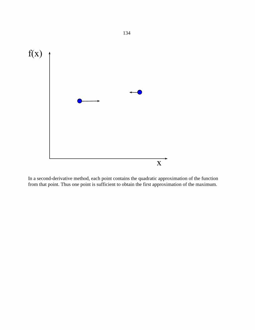
134

In a second-derivative method, each point contains the quadratic approximation of the functionfrom that point. Thus one point is sufficient to obtain the first approximation of the maximum.

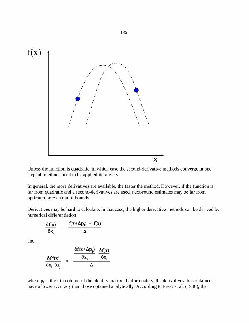
135

Unless the function is quadratic, in which case the second-derivative methods converge in onestep, all methods need to be applied iteratively.

In general, the more derivatives are available, the faster the method. However, if the function isfar from quadratic and a second-derivatives are used, next-round estimates may be far fromoptimum or even out of bounds.

Derivatives may be hard to calculate. In that case, the higher derivative methods can be derived bynumerical differentiation

and

where pi is the i-th column of the identity matrix. Unfortunately, the derivatives thus obtainedhave a lower accuracy than those obtained analytically. According to Press et al. (1986), the

136

number of significant digits in the derivatives calculated numerically cannot be higher than halfthe number of significant digits in the original function. In general the selection of ) is not an easyone.

Some popular maximization algorithmsDownhill simplex (derivative-free)

One of the most popular derivative-free maximization algorithms is downhill simplex. It isdescribed in the animal breeding context by Boldman et al (1995) in the MTDFREML manual.Let n be the number of parameters to find. Initially create n+1 vectorsx0, x1,.., xnand calculate the functions f(xi)=fi ordered so thatf0>f1>...>fn

Choices on the maximization for one dimension are shown below.

137

The general algorithm is

do until convergence Calculate the mean point: xm= ave(x1,..,xm)

Calculate a reflection of the worst point against the center point: xr = xm+"(tm-tp)

caseThe new point is best!fr > f0

Try even a better pointxb=xm+((xr-xm)xn=better(xr,xb)

The new point is neither worst nor bestf0 >fr >fpReplace the worst point

xp==xrThe new point is almost worst

fp-1 >fr >fpContract to the opposite side of the worst point

xp=xm+$(xr-xm)The new point is worst or equal

fr #fpTry contracting first to the worst point

xr=xm+$(xp-xm)New point betterfr > fp

xp=xrNew point worsefr <= fp

Contract in every direction towards the best pointxi=(xi+x0)/2 for i=1,..,n

end caseend do

Sample constants: "=1; $=.5; (=2

Powell (derivative-free)

138

Set the initial point xbasedo until convergence Find the “best” direction d by probing n dimensions Find " such that:

xnew = xbase + d"enddo

Fixed point (first derivative)

Rearrange the equationdf(x)/dx = 0

tox = g(x)

and solve asx(n+1) = g(x(n))

The choice of g is critical to convergence. For example, the rearrangement of

results in divergence, but a similar expression converges rapidly

Newton (second derivative)

x(n+1) = x(n) - [d2f(x)/(dx)2]-1 df(x)/dx

Quasi-Newton (first derivative)

When second derivatives are difficult to compute, they may be approximated from firstderivatives. A method that approximates the second derivatives by finite differences is calledsecant. For more information, see More and Wright (1993) or Woodford (1992)

139

Acceleration to EM (fixed point) estimates

The convergence rate in the EM algorithm can be slow, especially when the number of equationsrelative to records is high. Denote the EM algorithm as

In the single trait, the iteration would be similar to

And the convergence curve would be similar to

140

Thus in later rounds, the convergence would be predictable, similar to convergence of stationarymethods in the linear system of equations. Little (1987) has shown that the convergence rate in theEM algorithm is inversely proportional to the fraction of missing data. That fraction like thelargest eigenvalue of the iteration matrix is hard to compute analytically but can be approximatedduring the progress of iteration.

For a single component, Schaeffer (1979) showed how results from two separate cycles of the EMiteration can be used to extrapolate almost to the converged solutions. Misztal and Schaeffer(1986) have shown that the em(x) approximately follows the geometric progression, and that thefinal value can be extrapolated from estimates of successive rounds of EM iteration. Laird et al.(1987) presented similar ideas for multiple dimensions.

Function em(x) is locally linear near the convergence point. Therefore, for large n, we can write

Then

141

and finally

The extrapolation is beneficial only when the expression

becomes stable. Otherwise the extrapolation can deteriorate the convergence. Various types ofaccelerations of the EM algorithm have been used successfully in packages DMUEM, andREMLF90, with the reduction in the number of rounds by 2-10 times. Quasi-Newtonimplementation in VCE, where only the first derivatives of the restricted likelihood are computed,can be regarded as either approximated second-derivative algorithm, or accelerated EM.

142

Convergence properties of maximization algorithms in REML

Examine the cost of derivative and derivative-free algorithms in REML following Misztal (1995).Convergence rate can be described in terms of accuracy as a function of the number of rounds ofiteration (Minoux 1986). Linear convergence means linear relationship between accuracy andround of iteration, i.e., constant number of rounds is required for a gain of one extra digit ofaccuracy. The fixed point iteration (EM algorithm) seems to have a linear convergence. In asuperlinear convergence, each round of iteration results in increasingly larger gains in accuracy.Finally, in a n-step convergence, n steps are required to implement one round of iteration.

The convergence rate of maximization algorithms for general functions cannot be derived easily.However, it could be derived for quadratic functions, and any twice-differentiable function,including L, is locally quadratic. Then, the convergence of better derivative-free (DF) algorithmssuch as Powell or Rosenbrock is n-step superlinear (Minoux 1986), and is dependent on n, thedimension of the function being maximized. For better derivative (D) algorithms, such as quasi-Newton (first-derivative) or Newton-Raphson (second-derivative), the convergence is superlinearand does not depend on n (Bazaraa 1993; Minoux 1986). This leads to conjecture that better DFalgorithms converge, in general, n times slower than better D algorithms. N can be expressed interms of number of random effects, nr, and number of traits, nt, as:

n = (nr +1)nt(nt+1)/2 (4)

where the extra 1 is for the residual.

This difference in convergence rate is only approximate because differences exist within better Dor DF algorithms, and L is not quadratic. Also, more sophisticated methods may fail when thestarting point is far away from the maximum.

Cost of one step of D and DF in multiple traitsLet C be a coefficient matrix of the mixed model equations Assume that in DF, all computingresources are spent in computing |C|. Also assume that in D, all computing resources are spent infinding elements of C-1 corresponding to nonzero elements in C, or a sparse inverse of C. In densematrices, computing the inverse requires 3 times more arithmetic operations than computing thedeterminant alone (Duff et al. 1989). Both operations require an equal amount of storage. Approximately the same applies to the number of arithmetic operations in sparse matrices(Misztal and Perez-Enciso 1993). The amount of storage required is 3 times larger for sparseinversion if the inverse elements are computed by columns. Both options are supported underFSPAK.

In multiple traits, assuming that almost all traits are recorded, the coefficient matrix of themixed model equations has nt times more equations and an average equation has nt times morenonzero elements than in single traits. In dense matrices, the memory and computing requirementsfor inversion or computing the determinant for a matrix nt larger increase as nt

2 and nt3,

respectively. The same applies to sparse matrices, where memory and computing requirements

143

increase approximately as pq and pq2, where p is the number of equations and q is the averagenumber of nonzeroes per equation (Duff et al. 1989).

Cost of one unit of convergence relative to single trait estimation

Let C1d be the cost of one step of D in a single trait estimation. Let us compute costs of the same

level of convergence in nt traits for the DF and D algorithms: Cndf and Cn

d. If the DF convergenceis n times slower, computations for the matrix operations increase as nt

3, and computing thedeterminant costs a third of computing the inverse, the following formulas can be derived:

Cnd = nt

3 C1d (1)

Cndf = a (nr +1)nt(nt+1)/2 nt

3 C1d

= (nr +1) nt4(nt+1 )C1

d / 6 (2)and the relative costs are:

Cnd /C1

d = nt3 (3)

Cndf / C1

d = (nr +1) nt4(nt+1 )/6 (4)

. (nr +1) nt5/6 (5)

Cndf /Cn

d = (nr +1) nt(nt+1 )/6 (6) . (nr +1) nt

2/6 (7)

According to equation (3), the number of numerical operations in D increase cubically with thenumber of traits. In equation (4), the cost of DF increases with the fifth power of the number oftraits. From equation (1) one can find that the costs of DF and D in models with 2 random effectsare similar in single trait. DF is less expensive with 1 random effect, and D is less expensive withmore than 2 random effects. In multiple traits, DF is nt

2 more expensive than D.Relative costs of multitrait DF REML evaluation using DF and D algorithms, computed

with formulae (3) and (4) are presented below

Number of traits Number of arithmetic operations Memoryrequirements

DF D

1 1 1 1

2 24 8 4

3 162 27 9

4 640 64 16

5 1875 125 25

144

6 4536 216 36

The table below shows time to calculate multiple trait REML estimates assuming that D and DFboth took a minute in single traits.

Number of traits Approximate CPU Time

DF D

1 1 min 1 min

2 ½ hr 8 min

3 2½ hrs ½ hr

4 11 hrs 1 hr

5 > 1 day 2 hrs

6 3 days 3½ hrs

Accuracy of the D and DF algorithms

In DF, if L(1) is computed with r significant digits, then 1 can be bracketed with at most r/2significant digits (Press et al. 1989). Such a limit does not exist in D. Worse numerical accuracyof the DF maximization is illustrated with in the Figure below, which shows a quadratic functionand its derivative.

145

y = -x2 + 2x - .6

dy/dx = -2x+2

The function is very flat, and the maximum of the function cannot be determined accurately bylooking at the function alone. The maximum can be determined much more precisely by finding azero of the function's first derivative.

Loss of accuracy in DF does not appear a problem at first. Most computations are done withdouble precision, which corresponds to 15-17 significant decimal digits, and estimates with 1% or2 significant digits of accuracy are considered sufficiently accurate in practice. However, thelikelihood function can have low accuracy for a variety of reasons. Some accuracy is lost due to aroundoff error when summing all components of L. Components of that function may havereduced accuracy. This particularly applies to the determinant, where the loss of accuracy couldresult from lack of pivoting in Cholesky decomposition-based packages, poor conditioning of thecoefficient matrix and rounding errors associated with computing in large matrices. In multipletraits, the coefficient matrix of the mixed model equations is composed of R0

-1and Gi0-1 -

covariance matrices between traits for residual and random effect i, respectively. Poorconditioning of these matrices results in poor conditioning of W and subsequently low accuracyof determinants and traces. R0

-1and Gi0-1 would be poorly conditioned numerically when traits are

highly correlated or linearly dependent. The loss of accuracy due to poor conditioning of C is alsopresent in derivative maximization, but it has smaller effect on the estimates because of betternumerical properties of the derivative maximization.

146

Another source of inaccuracy could arise in algorithms where derivatives are obtained numericallyby differentiation. For example, the Quasi-Newton algorithm can be so implemented in DF, andone can regard other DF algorithms as using the numerical differentiation implicitly. The accuracyof such differentiation is dependent on the step side and could be very low for steps too large ortoo small. Subsequently, the accuracy would be dependent on parameters that define the step size,and in particular could be good for some problems but poor for others.

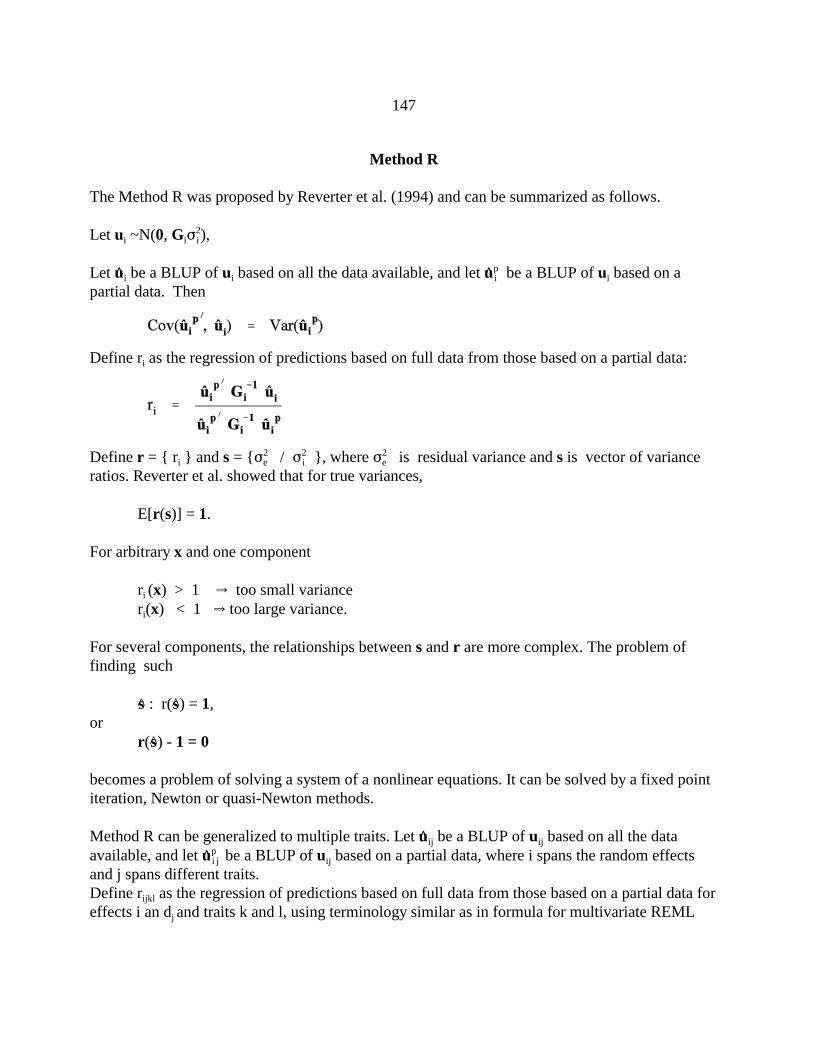
147

Method R

The Method R was proposed by Reverter et al. (1994) and can be summarized as follows.

Let ui ~N(0, GiF2i ),

Let ui be a BLUP of ui based on all the data available, and let u i p be a BLUP of ui based on a

partial data. Then

Define ri as the regression of predictions based on full data from those based on a partial data:

Define r = { ri } and s = {F2e / F2

i }, where F2e is residual variance and s is vector of variance

ratios. Reverter et al. showed that for true variances,

E[r(s)] = 1.

For arbitrary x and one component

ri (x) > 1 Y too small variance ri(x) < 1 Y too large variance.

For several components, the relationships between s and r are more complex. The problem offinding such

s : r(s) = 1, or

r(s) - 1 = 0

becomes a problem of solving a system of a nonlinear equations. It can be solved by a fixed pointiteration, Newton or quasi-Newton methods.

Method R can be generalized to multiple traits. Let uij be a BLUP of uij based on all the dataavailable, and let u i

pj be a BLUP of uij based on a partial data, where i spans the random effects

and j spans different traits. Define rijkl as the regression of predictions based on full data from those based on a partial data foreffects i an dj and traits k and l, using terminology similar as in formula for multivariate REML

148

For arbitrary x and one component rijkl (x) > 1 Y F2

i jkl too smallrijkl(x) < 1 Y F2

i jkl too large.No exact formulas are available for the residual variance but quasi-REML approximations wereused by Reverter et al. (1994) as follows

where nri is the number of records in trait i, and

where nrij is the number of records with both traits i and j recorded.

Method R is potentially less expensive than other methods because it only requires solutions tothe mixed model equations. Aside from being feasible computationally, Method R has severalother desirable properties. First, at least in single traits it returns estimates within the parameterspace. Second, it is resistant to bias caused by assortative mating because it considers therelationship matrices. Also, it has been shown to be as resistant as REML to selection caused bynon-random replacements (Snelling, 1994) and incomplete reporting (Kaiser et al., 1996); Cantetand Birchmeier (1998) initially reported bias under selection but later discovered that it was due toan error in programming. Disadvantages of Method R would include a larger sampling variancethan other methods for the same data set, however, this disadvantage can be compensated by theability of Method R to consider much larger data sets.

Recently, Druet et al.(2001) has found that rijkl for covariances has a discontinuity because both itsnominator and the denominator can have a value of 0. They suggested alternative formulas. Exactformulas for Method R in multiple traits are unknown.

Selection of partial data

The regressions do not specify which subset of data is selected. If subset is either a very small or avery large percentage of the complete data set, up’s will either be close to 0 or to u’s, and theregressions will have very large sampling error. Thus a size of 50% seems to be the a good choice.Also by inappropriate selection of records, one can create bias for the model with the reduced data

149

set. A few types of subsets can be considered:a) random,b) by truncation over timec) by truncation over later records with repeated records.

Random selection seems to be attractive, especially that subsets can be easily changed bychanging seed in a random number generator, and sampling variance can be approximated asvariance of the samples.

Method R can have poor properties when the model does not contain all fixed effects. Forexample, in the study by Misztal et al. (1997), heritability for stature with single record per animalwas 44%. When multiple records were considered, the heritability has increased to almost 70%.After adding the adjustment for age, the heritability dropped to 45%.

In simple models (Duangajinda et al., 2001), Method R has been shown to be mostly unbiased.Biases were present with small data sets and with phenotypic selection across but not withincontemporary groups.

Numerical considerations

When the problem is small enough so that LHS can be factorized, REML would provide betterestimates than Method R. Therefore the value of Method R is in larger problems where solutionscan be obtained only by iteration. For calculation of breeding values, the accuracy of solutions isusually not critical, and an accuracy of 2 decimal digits is more than satisfactory. For method R,convergence to

r=1±0.0001 was found to be corresponding to the accuracy of the estimates of

s±5%Thus, r=1±0.0001 or calculated with at least 4 decimal significant digits should be considered theminimum. To get that accuracy, the solutions to MME should be calculated with even higheraccuracy, 5 to 6 significant digits. Otherwise convergence of Method R may not be achieved.

Because Method R results in a problem of solving the nonlinear system of equations, theconvergence of this method is more similar to D than to DF.

Solution of the nonlinear system of equations by Secant

The problem of findings : r(s) = 1

was solved by the secant method, which initially is equivalent to the Newton method, wherederivatives are computed by numerical differentiation. This algorithm is equivalent to assumingthat

150

r = As +bConsequently, approximate solutions are obtained setting r =1

A and b can be found when n+1 pairs of {s(i),r(s(i))} are available. Then,

r(s(i+1)) - r(s(i) )= A [s(i+1) - s(i)]

denoting)s = [s(1 )- s(0), s(2 )- s(1), ..,s(n )- s(n-1)])r = [r(s(1)) - r(s(0)), r(s(2)) - r(s(1)), ..,r(s(n)) - r(s(n-1))]

the equation can be written as)r = A )s

ThusA = )r ()s)-1

b can be computed from the last pointb = r(s(n)) - A s(n )

which will result in

The algorithm contains heuristics to ensure the convergence of the algorithm that would otherwiseresult in estimates out of the parameter space or in a slower convergence rate.

1. Choose an initial guess s(0);2. Assign n extra points as follows:

s(1) = s(0) + [*1,0,...,0]’s(2) = s(1) + [0,*2,0,..,0]’......s(n)

= s(n-1) + [0,0,..,*n]’.

3. Compute {r(s(i))}, i = 0, n;

4. Compute differences:)s = [s(1 )- s(0), s(2 )- s(1), ..,s(n )- s(n-1)])r = [r(s(1)) - r(s(0)), r(s(2)) - r(s(1)), ..,r(s(n)) - r(s(n-1))].

5. Compute next-round solutionss(n+1) = s(n) + )s ()r)-1 [1 - r(s(n))]

5. Limit changes if too large:

151

maxchange = max( |si(n+1) - si

(n)| / |si(n)|)

I

if maxchange >( then s(n+1) = s(n) +(/maxchange (s(n+1) - s(n)).

6. If change large, compute n new points as before; if changes small, use all but one last point.

if max{|ri(s(n+1)) - 1|} > , then i

if max|si(n+1) - si

(n)| / |si(n)| > 8

I set s(0) = s(n+1)

goto 2 else s(0) = s(1), s(1) = s(2), ..,s(n-1) = s(n), s(n) = s(n+1) goto 3.7. Optionally, refine s using previously computed matrices

s(n+1) = s(n+1) + )s ()r)-1 [1 - r(s(n+1))].

In program JAADOM, changes between samples *i were chosen to correspond to a change ofvariance of Fe

2/200, maximum relative changes were limited to ( = 0.7, the stopping criterion was ,= 0.0001, and changes were regarded as small for 8 = 0.1.

Numerical example s(0) = [ 0.6, 0.9]’ s(1) = s(0) + {-0.0017946 ,0,...,0} = [0.5982054, 0.9]’ s(2) = s(1) + {0,-0.00403189 ,0,..,0} = [ 0.5982054, 0.89596811]’

r(s(0)) = [1.008687, 1.009935]r(s(1)) = [1.008587, 1.009897]r(s(2)) = [1.008552, 1.009800]

s(n+1) = [ 0.4940763 0.5808855]’

r(s(n+1) ) = [1.000021 0.9973247]’.

Because

152

1 - 0.9973247 = 0.0026753 > 0.0002, s(0) is set to s(n+1), and computations are repeated from step 2. After that, the procedure converges at

s(n+1) = [0.4791, 0.6592]’ where

r(s(n+1)) = [1.00008, 0.99981]

It would be worthwhile to find out whether better performance could be obtained by quasi-Newtonmethods..

153

Bayesian methods and Gibbs sampling

Following Wang et al. (1993), in the single-trait model

the conditional distribution which generates the data is

with the density

One can specify distributions for $, u’s and F’s. The distribution of $ is flatp($) % constant

The distribution for u’s is multivariate normal

with the density

and for the variance components, it can be scaled inverted P2

where s..2 is the prior value and <.. can be viewed as the degree of belief (uniformative prior for

<..=0). The joint posterior density with flat priors is

or

154

Information about variance components could be obtained from marginal distributions byintegrating all unnecessary effects/parameters out

From the marginal posterior distribution one can calculate mean, mode, standard deviation orconfidence intervals.

For realistic models, the analytical integration is hard or impossible.

Gibbs sampling (Geman and Geman, 1984) is an easy although computationally-intensive methodof numerical integration of likelihoods whenever conditional distributions are easy to compute. Themethod would progress as follows:

1. Assign priors to

2. Sequentially calculate samples from conditional distributions

...........................

...........................

155

...........................

Elements of $ or u can be sampled either as by vector or by individual elements.

3. Calculate 2. repeatedly. After a period of burn-in, samples generated above will be from theirrespective marginal distributions.

The conditional distributions are constructed by assuming the conditional parameters fixed and bydropping terms from the posterior density that are dependent on conditional parameters only. Thus,the conditional posterior density for $ is

This corresponds to the distribution

or

and finally

Similarly, for the i-th random effect ui the distribution is

where

For the residual variance, the full conditional density is a scaled inverted P2

156

with the distribution

where

and

For the other variance components, the distributions are similar

with the distribution

where

and

A multivariate distributions for a complete fixed or random effect is hard to obtain. However, adistribution for a single level of a fixed or random effect is simple. Let

$ = {$i}, i=1,mand

The conditional marginal density for $i is

157

where y($i) are records containing $i only, and Zj($i) corresponds to y($i). The corresponding

distribution is

or

which can be further simplifying by expressing the last equation in terms of RHS and LHS of theMME

The expression for the mean is a solution in the Gauss-Seidel iteration. A similar distribution can beobtained for j-th level of random effect i: uij

Example

Consider the sire modelyijk = gi + sj + eijk

158

and the data

i j yijk

1 1 3

1 1 4

2 1 5

2 1 6

2 2 7

Assume priors:g=s=0, F2

e =1, F2s=.1

The mixed model equations are:

The initial distributions are

g1|... ~ N(7/2, 1/2), for example sampled as 4g2|... ~ N(18/3, 1/3), for example sampled as 6s1|... ~ N[(18-2*4 -2*6)/14, 1/14], for example sampled as -.2s2|... ~ N([(7-1*6)/11, 1/11], for example sampled as .3

e’ = [ (3-4- -.2), (4-4- -.2), (5-6- -.2), (6-6- -.2), (7-6-.3)] = (-.8, .2, -.8, .2, .7)e’e=1.85

F2e|... ~ 5 * 1.85/5 P-

52, for example sampled as 1.1

u’u=.13F2

u|... ~2 * .13/2 P-2

2, for example sampled as .05

The next round distributions will beg1|... ~ N[(7-2*-.2)/2, 1.1/2], for example sampled as 3.5g2|... ~ N[(18-2*-.2-.3)/3, 1.1/3], for example sampled as 5.5s1|... ~ N[(18-2*3.5 -2*5.5)/15, 1/15], for example sampled as .1s2|... ~ N([(7-5.5)/12, 1/12], for example sampled as .2

159

and so on.

Using the Gibbs sampler

Typically, samples from the Gibbs sampler would show an initial period of burn-in, followed by a repetitive pattern. This is shown in the idealized chart below; the real curve would not be as smooth.

The burn in period lasts usually between 500 and 10000 samples, although for slowly convergingsampler that number could be considerably higher. One way to determine the burn-in period is tostart two chains with the same random number generators but different priors.

160

Convergence of the two chains indicate the end of the burn-in. Repetitive pattern that follows theburn-in period is due to the largest eigenvalue of the iteration matrix, and its length is dependent onthe model and data structure. Because of repetitions, the subsequent samples are correlated, and inorder to make inferences about parameters of the model, it makes sense to analyze only every nsample, where n can be from 10 to 1000. Selected samples can be used to create an approximatemarginal density, where the accuracy of the approximation will depend on the number of samplesand on the correlation of subsequent samples. The approximate density could look as follows

The total number of samples necessary to plot a density could be as high as 1 million. Fewersamples are needed to estimate a mean or a mode of the distribution.

161

Multiple-traits

In multiple traits, the marginal distributions for u’s and $’s can be obtained as in single traits, byusing an analogous of the Gauss-Seidel iteration. For variances, a univariate inverted chi-squaredistribution becomes a multivariate inverted Wishart distribution.

For simplicity, assume a t trait model with a single random effect. Denote ui and ei as i-th traitrandom samples for the random effect and the residual, respectively. The distribution for thevariance components of the random effect is

where ng is number of levels in the random effect, <g is degrees of belief (equal to -t-1 for flatpriors), and

The distribution for the residual variance components is

where n is the maximum number of records (including missing), <e is degrees of belief (equal to -t-1for flat priors), and

If some records are missing, they are predicted from the distribution

“missing records”|u,$, R,G,”known records”

each round and then used as if they were known. Let subscript m denote quantities associated withmissing traits, and p associated with present traits. The missing records can be predicted as:

ym ~ MVN[E(ym|....),Var(ym|...)]

with

162

E(ym|...)=Xm$ + Zmu +RmpRpp-1(yp-Xp$ + Zpu)

Var(ym|...)=Rmm-RmpRpp-1Rpm

Convergence properties

The Gibss sampler’s convergence is tied to the convergence of the method of Gauss-Seidel, and topriors. When the corresponding convergence of Gauss-Seidel is slow, the convergence of the Gibbssampler will be slow too. One way to increase the convergence speed in multiple traits is to useblock iteration, where samples are generated by block of traits.

The Gibbs sample may diverge with certain priors. For example, uninformative priors for variancecomponents (<=0) are often worse than flat priors (<=-t-1).

Computing implementations

The Gibbs sampler require a large number of rounds. Therefore, its efficiency is quite important. Inthe most obvious implementation, the LHS is recreated each round, with procedures to set up theequations taking perhaps as much as 95% of computing time. Also, memory requirements may befairly steep. Several algorithms to cut time and memory are possible although some of them are hardto implement for complicated models. In all cases, the data can be stored in memory or read by fastroutines.

Single trait models

In single traits, when working with variance ratios, only the part of the LHS due to (co)variancematrices changes. If the part of LHS due to records and the relationship matrices are kept in memoryseparately, each equation can be reconstructed by combining these matrices and the current varianceratios, without recomputing the LHS.

Multiple trait models with same model per trait

In this case, only the structure of the LHS for single trait needs to be stored, and the multiple-traitLHS is reconstructed dynamically using the current (co)variance matrices, as in the previous case. Ifsome traits are missing, the data needs to be read every round to recreate the missing traits, but theLHS is not affected.

Other multiple trait models

In large multitrait models, contribution from relationship matrices can be much larger thancontributions from records because single-trait numerator relationship matrices need to be

163

duplicated over for all combinations of traits and possible sets of correlated effects. To reducestorage and computations, only the contributions from records can be stored, and contributions frompedigrees can be recreated from a single-trait copy of the numerator relationship matrix.

Alternately, the model can be redefined so as to have the same model per trait. For example, let themodel be identical except for different fixed management effect m in the i-th trait:

yi = Ximi+....

Redefine that model so that for each trait management effects from all traits are present:

yi = X1m1i + X2m2i + Ximii ....

and treat the effects as random with (co)variances:

Variance close to 0 cause an effect to disappear while variance of infinity makes an effect fixed; Inpractical implementation, values of a should be very high and b very small but in a range so thatnumerical errors can be avoided. Also, the Gibbs sampler need to be modified not to samplevariances of m.

Large models

One possibility with large data is by iteration-on-data by Gauss-Seidel, as discussed in an earlierchapter. Several copies of the data and relationship files may be needed. Programming may becomequite complicated for complex models but is simple for simple models.

General models

Updating MME in linked-list form may be time consuming. Matrices in HASH format are faster toset up, but they need to be converted to IJA format so that rows of the LHS are availablesequentially. Both creation of the hash matrix for the first time and conversion to the IJA formattake time. Schnyder (1998, personal communication) noticed that, after the first round, the structureof the matrices in the IJA and HASH does not change; only values change. He suggested thefollowing algorithm:

a) after the first round, create links to facilitate fast conversion between HASH and IJAstructures,b) before every consecutive round, only zero HASH values but not indices.

In the end, the creation of the LHS can be 2-3 times faster without sacrificing any modeling

164

flexibility.

165

Ways to reduce the cost of multiple traits

In t traits, the computing costs increase as follows

Approximate Cost

Arithmetic Operations Memory

solutions iterative finite

>t2

t3t2 t2

REML Derivative-free Derivative

t5

t3t2 t2

The cost of obtaining iterative solutions includes the cost of increased number of rounds because ofa lower convergence rate, which is especially low when traits are missing.

Canonical transformation

Let the t-trait model be

with

where G0 and R0 are the t x t variance-covariance matrices. For individual trait i, the model is

where X* and Z* are single-trait design matrices, same for all traits. The covariances between thetraits are

For any symmetric semi-positive-definite G0 and R0 there is a transformation M such that

M G0 M’ = D and M R0 M’ = I

166

where D is the diagonal matrix. For each record j, the vector of observation is

Multiply each vector of observation by M

which for all observations can be written as

Then, the model becomes

with variances

where the transformed traits are uncorrelated. For each transformed trait i

with covariances between the traits

and the mixed model equation for each trait i are

Thus, the single-trait equations after the canonical transformation are uncorrelated and can besolved by single trait procedures. To compute the solutions on the original scale, back transform

Note that the canonical transformation can be performed only when the following apply:- same model for all traits- no missing traits for any observation- single random effect

The transformation matrix can be constructed as follows. Decompose Ro into eigenvectors andeigenvalues

167

Then decompose again

The transformation matrix is

For verification

Canonical transformation and REML

Estimation of REML by canonical transformation can be done by the following steps:a) Assign priors for R0 and G0b) Find transformation and transform the datac) Estimate single-trait variance componentsd) Combine the estimates; the formulas below assume the first-derivative algorithm

where nr is number of records, ng is number of levels in the random effect, and Cm,i is the

168

block of the inverse of the coefficient matrix corresponding to random effect i. Form

The new estimate of (co)variance components on the original scale are

e) If no convergence, repeat from b)

Contrary to general model REML, the cost of canonical transformation REML is only linear withthe number of traits, and there is no increase in memory over single-trait. However, all limitationsof the canonical transformation apply.

Numerical properties of canonical transformation

With many traits, some traits are likely to become almost linear functions of the other traits.Therefore, matrices R0 and G0 may became almost singular, and the whole coefficient matrix canbecome almost singular. This can easily be shown for a mixed model. The condition number of amatrix is defined as

cond(B)=|B| |B-1| where higher condition numbers are associate with poorer numerical properties. In a generalmultiple-trait fixed model, the coefficient matrix is

with the condition number

Similar increase in condition number occurs in mixed models, where that condition is also afunction of G0 but it is more difficult to show analytically. High condition number of a matrix leadsto numerical errors in the factorization, or to extremely low convergence rate in iterative methods.In variance component estimation, the computed rank of the coefficient matrix may change fromround to round.

In the canonical transformation, the coefficient matrix in the fixed model is X’X

and thus its condition is independent on R0.

In canonical transformation, the near singularity R0 and G0 shows in elements of D and Dr beingalmost 0. Computer program MTC contains the following heuristics with respect to the canonical

169

transformation. For the residual eigenvalues:

and for the “random effect eigenvalues”:

While general-model REML by any algorithm for more than 3-6 traits isn’t usually stablenumerically, the canonical transformation REML was known to be successful for 32 traits!

Extensions in canonical transformation

Multiple random effects

Extend the model to p multiple random effects

with

We need such a transformation that

M R0 M’ = I and

M G0k M’ = Dk, k=1,p

where Dk are diagonal matrices. In general, such a transformation does not exist for p>1. Lin andSmith (4) hypothesized that in practical situations an approximate equation can hold

M G0k M’ . Dk The algorithm to calculate M would be similar as before

W and Di in the decomposition

can be obtained approximately by the FG algorithm (Flury, 1988)The transformation matrix is

For a good approximation, matrices G0k must be alike. In general multiple traits with t traits and p

170

random effects, the total number of parameters to estimate is:p t (t+1)/2

With the approximation, the number of parameters would be(p-1) t +t(t+1)/2

For 2 random effects and 4 traits, the number of parameters is 20 in the first case and 14 in thesecond case.

Misztal et al. (1993) has obtained very good results with the approximation for type and milk traits.This indicates that the multiple-trait variance-covariance structure in several random effects issimilar. Reversely, in that case, general REML would estimate more parameters than necessary.

Missing traits

Ducrocq and Besbes (1993) have developed a method to apply the canonical transformation whenrecords on some traits are missing. Let ym be the m-th observation partitioned as (ym", ym$), whereym" was recorded but ym$ is missing. Denote the model for each part as

Let (k) denote the current round of iteration. Missing record ym$ can be predicted using the equation

where R0,"$ is a block of R0 corresponding to traits " and $, and R0,"" is a square block of R0corresponding to trait ".

To solve the mixed model equations, in each round predict missing records and use them for oneround of iteration as if they were known. Then, using the new estimates, predict the missing recordsagain. Continue until convergence.

Canonical transformation with missing traits requires that in each round the previous roundestimates be untransformed, data read, the missing records predicted, and all the recordstransformed.

Formulas to apply the modification for missing records to REML has not been derived. Thus, theprocedure is applicable only for obtaining the solutions.

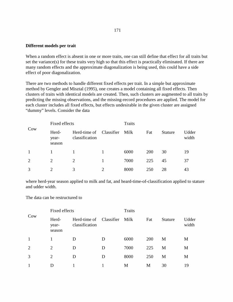
171

Different models per trait

When a random effect is absent in one or more traits, one can still define that effect for all traits butset the variance(s) for these traits very high so that this effect is practically eliminated. If there aremany random effects and the approximate diagonalization is being used, this could have a sideeffect of poor diagonalization.

There are two methods to handle different fixed effects per trait. In a simple but approximatemethod by Gengler and Misztal (1995), one creates a model containing all fixed effects. Thenclusters of traits with identical models are created. Then, such clusters are augmented to all traits bypredicting the missing observations, and the missing-record procedures are applied. The model foreach cluster includes all fixed effects, but effects undesirable in the given cluster are assigned“dummy” levels. Consider the data

CowFixed effects Traits

Herd-year-season

Herd-time ofclassification

Classifier Milk Fat Stature Udderwidth

1 1 1 1 6000 200 30 19

2 2 2 1 7000 225 45 37

3 2 3 2 8000 250 28 43

where herd-year season applied to milk and fat, and heard-time-of-classification applied to statureand udder width.

The data can be restructured to


Herd-year-season

Herd-time ofclassification


1 1 D D 6000 200 M M

2 2 D D 7000 225 M M

3 2 D D 8000 250 M M

1 D 1 1 M M 30 19

172

2 D 2 1 M M 45 37

3 D 3 2 M M 28 43

where M denotes missing trait and D denotes the dummy effect. For example, if herd year seasonhad 100 levels, and herd-time-classification had 1000 levels, D=101 for herd-year-season andD=1001 for herd-time-classification. Because the herd effects do not overlap, they can be joined toreduce storage


Herd-year-season orHerd-time ofclassification


1 1 D 6000 200 M M

2 2 D 7000 225 M M

3 2 D 8000 250 M M

1 1 1 M M 30 19

2 2 1 M M 45 37

3 3 2 M M 28 43

This method may be an approximation because the residuals of different clusters are assumeduncorrelated.

Another method was proposed by Ducrocq and Chapuis (1997). Define all effects for all traits. Let$ be solutions to all the fixed effects where all fixed effects are applied to all traits, and let $c besolutions constrained so that solutions to fixed effects that should be absent for certain traits are 0.

Find such a transformation P so that$c = P$

and then find an equivalent transformation on the canonical transformation side

Solve iteratively using all the fixed effects, and the end of each round apply the abovetransformation, either on the original or on the transformed scale.

173

Implicit representation of general multiple-trait equations

Tier and Graser (1991) presented a way to drastically reduce the amount of storage for multiple-traitmixed model equations. Initially assume that all traits follow the same model but some traits aremissing, and that there is only one random effect. For each missing trait combination i, the mixedmodel can be written as

The left hand side of the mixed point equations can be written as

where Ro(i) is the inverse of the residual (co)variance matrix for a missing trait combination i. For t

traits, the memory needed to store the coefficient matrix can be close to t2 greater than that for singletraits because scalars in single trait are being expanded to txt blocks.. Each txt block correspondingto the jk-th single-trait equation can be computed as

Instead of storing the complete coefficient matrix, it is sufficient to store C={cjk}. Each vector cjk

174

contains counts of “kernels”, and it has as many elements as there are combinations of missingeffects in the data + 1. In a 5-trait situation, where there are five patterns of missing traits, each txtblock would require the storage of 15 elements, and the corresponding vector c only 6 elements.The storage requirements can drop further if counts are kept by 2-byte or even 1-byte numbers asopposed to 4- or 8-byte real numbers for the coefficients.

The method can be further refined if one creates a list of all txt blocks that are present in thecoefficient matrix, and each entry in the coefficient matrix is a pointer to an element in this list.

Example

Consider the modely = Hh + Za + ewhere h is the herd effect, a is the animal effect, and the data is

animal sire dam herd milk protein somaticcell score

1 4 3 1 10,000 300 300,000

2 4 - 1 12,000 - -

2 4 - 2 13,000 - -

3 - - 2 13,000 350 -

3 - - 2 11,000 - -

4 - - 2

The data contains 3 classes of missing effects:

class missing1 none2 somatic cell score3 protein and somatic cell score

The matrix C would contain the following vectors when shown upper-stored

1 0 1 0 1 0 0 0 0 0 1 0

0 1 2 0 0 0 1 0 0 1 1 0

1 0 0 2 0 0 0 -1 0 0 0 -1

175

0 0 2 1.33 0 0 0 -.66

0 1 1 1.5

0 0 0 1.86

176

Because many vectors would appear more than once, one can store the matrix C as links and a list.

1 2 3

4 3 5

6 7 7

8 9

10

11

list

1 1 0 1 0

2 1 0 0 0

3 0 0 1 0

4 0 1 2 0

5 0 1 1 0

6 1 0 0 2

7 0 0 0 -1

8 0 0 2 1.33

9 0 0 0 -.66

10 0 1 1 1.5

11 0 0 0 1.86

Most likely, only a few elements in the list will occur in most of the entries. Solutions by blockiteration would involve Cholesky decomposition of diagonal blocks cjjR*. Because some of theblocks can occur many times, computer time may be saved by precomputing the Choleskydecomposition for all types of blocks on the diagonal of C.

The above technique complicates when models for each trait are different. For specialconsiderations in such a case, see the work by Tier (1992).

177

Computing in genomic selection

In genomic selection (Meuwissen et al., 2001), animals are genotyped by large panels of SNP,effects of SNP markers or haplotytype segments based on those markers are predicted, and thosepredictions are used to estimate genomic breding values for young animals based on theirgenotypes. At this time (2008), analyzes involve a few thousand high-reliability animals and up to60,000 SNP markers or haplotype segments.

A few types of models can be used to predict genomic breeding values (VanRaden, 2008, JDS).Two of them are shown using simplifications for clarity. In the first type one estimates genomiceffects in a simple model:

where y are (possibly deregreesed) proofs of high reliability animals, u are effects of individual SNPor haplotype effects, Z is a matrix relating animals to markers; var(u)=Du or IF2

u, var(e)==De or IF2e;

Dx are diagonal matrices. The genomic prediction a of animals based on the predicted effects is:

where Za is a matrix relating animals in a to respective SNP or haplotype effects.

Legarra and Misztal (JDS 2008) looked at methods to compute solutions to u. Because the systemequations is dense, setting it up requires large amount of memory + computations. For example, ifthere are 50,000 effects in the model, the number of different contributions to the system ofequations resulting from one observation is 50,0002 = 2.5*109 and the amount of memory requiredis > 10 Gbytes (half storage + double precision). One can avoid large storage by using the iterationon data. Such iteration with the PCG algorithm is very fast. The iteration on data using the regularGauss-Seidel in a straightforward implementation such as below is very slow:

where zi is the i-th a column of Z, uj is the j-th solution and dj is variance ratio for the j-th solution;

for simplification : has been removed from the model and ui on the right side is the most up-to-datesolution. The slowness is due to the large number of effects in the summation: 10,000 or biggerrather than a typical 10 in a regular animal model. Janns and de Jong (1999) noticed that:

Subsequently, the iteration can be implemented much faster as:

178

but after computing every solution, the estimated residuals need to be updated:

where )uj is the change in the value of uj.

In the second type, the genomic information is used to predict a genomic relationship matrix G.Then,

where D is a diagonal matrix related to heritability reliabilities, A is constructed as:

where P is a matrix containing genotype probabilities and " is a normalizing constant to ensure thatdiagonals for noninbred animals are close to 1.0. See Van Raden (2008) for more details.Computations in the second type include multiplications of large matrices. While constructingmatrices for the second form is expensive, they are similar for different traits. Also, the finalmatrices are smaller if the number of animals is much smaller than the number of SNP

Dense matrix computations benefit from vectorization, where operations involving large vectors canbe computed much faster (per element) than individual elements due to pipelining in modernprocessors. They can also benefit from parallelization, where computing is distributed amongseveral processors; computer chips available currently often have 2 to 4 processors. The use ofvectorization or parallelization can be automatic, through a compiler option, or manual. A section ofthese notes contains a short description of a manual parallelization using an approach calledOpenMP.

179

Data manipulation

So far we assumed that the data are available in an ordered way, with all effects numberedconsecutively from 1. A substantial part of data analysis is selection of records, data checks andrenumbering.

Renumbering

Data for mixed model programs require consecutive coding. Each effect should be coded from 1 tothe last level, without gaps. One of the more difficult renumbering is for the animal effect.The purpose of that ordering is:

1. Detection of discrepancies in pedigrees- parents too young or too old than progenies- animal as both male and female,- too many progenies per female

2. Elimination of unnecessary animals- animals without records and

without progeny, orwith one progeny and no parent

3. Assignment of unknown parent groups (if desired)

4. Actual renumbering in the formatanimal code; sire code; dam code; parents’ code.The parents’ code tells how many animals have been replaced by unknown parent groups. Itis desirable to code animals with records first because in that case the permanentenvironmental effect (in the repeatability model) can share coding with the animal effect.

5. Renumbering the animal id in the performance file. If the maternal effect is present, it needs to beadded to the performance file and a code for missing dams assigned for a record of an animal whosematernal information is unavailable.

Memory consideration

If one prepares a subset of the data, e.g., for a REML analysis, the number of animals in thepedigree file can be much larger than the number of animals in the performance file because ofmany noncontributing animals. The size of pedigrees can be limited if one considers animals in thefollowing order:

180

- animals with records- parents of above animals- parents of above animals- .....................................

or from the youngest animal to the oldest. The removal of unnecessary animals can then proceed inthe reverse direction, from the oldest to the youngest.

There are two basic methods of renumbering:A. by look-up tablesB. by sorting and merging

A. Look-up tables

Pseudo-program

Open performance fileLoad all animals with records into memorySort pedigree file by year of birth descendingFor each pedigree record

If animal in memory, load parents, year of birth, and possibly other info; accumulate #parents and #progeny

Sort animals in memory by year of birth ascendingFor each animal

If noncontributing Remove,Eliminate contributions of current animal to parents and progeny

If desired, calculate inbreeding and/or unknown parent groupsWrite renumbered pedigree fileOpen performance fileFor each record

Substitute original animal id by consecutive numberIf desired, add inbreeding and/or maternal fieldsWrite record

For fast search, the "hash" is about the most efficient.

Look-up approach is fast but memory intensive:10-50 bytes of memory per animal,10-50 Mbytes per 1 mln animals

181

B. Sort and merge

1. From pedigree and data files, extract animal id with estimated year of birth and code, which isone of a) has record, b) has pedigree record, c) has progeny

2. Sort by animal id

3. Summarize single entry per animal with:number of records,number of parentsnumber of progeny

4. Remove noncontributing animals5. Assign consecutive numbers, first to animals with records6. Sort data file by animal,7. Sort pedigree file by animal; merge in animal consecutive number8. Sort pedigree file by dam, merge in dam consecutive number9. Sort pedigree file by sire; merge in sire consecutive number

Sort and merge renumbering:need very little memory but plenty of disk spacespeed dependent on sorting!

Examples

182

animal a2 is redundant!

animal dam sire year of birth recorda1 a0 - 80 10a4 a1 a3 85 15a5 a4 - 90 12

sire pedigree filebull dam sire year of birtha2 - - 75a3 a0 a2 80

Required unknown parent group allocations

year of birth of youngestprogeny

unknown parent group

<85 1

$85 2

Contents of look-up table after loading animals with records (order dependent on search algorithm)

183

animal #parents #progeny #records birth #number

a1 0 0 1 80 1

a4 0 0 1 85 2

a5 0 0 1 90 3

Contents of look-up table after loading parents and parents of parents of animals with records

animal #parents #progeny #records birth #number

a1 1 1 1 80 1

a0 0 2 0 75 4

a4 2 1 1 85 2

a3 2 1 0 80 5

a5 1 0 1 90 3

a2 0 1 0 75 (none)

The last animal is noncontributing and can be eliminated. Renumbering of the pedigree done by onepass through the pedigree file. Unknown parents initially are assigned the birth year of their oldestprogeny

animal dam sire year of birth1 4 (80) 802 1 5 853 2 (90) 905 4 (80) 80

4 (75) (75) 80 year of birth predicted as year of birth of progeny - 5

Unknown parent groups are replaced by consecutive numbers after the highest animal number, andthe code shows the number of unknown parents

animal dam sire code1 4 6 12 1 5 03 2 7 15 4 6 1

184

4 6 6 2

The records’ file with animal id and records is created by reading the records file again and mergingthe animal id with the animal consecutive number

animal record1 102 153 12

Sort and Merge approach

First file:

animal type of entry year of birtha1 record&ped 80a0 dam 80a4 record&ped 85a1 dam 85a3 sire 85a5 record&ped 90a4 dam 90a2 sire_ped 75a3 sire_ped 80a0 dam 80a2 sire 80

After sorting by type of entry within animal:(rec = record. pedx = pedigree record with x known parents)a0 dam 80a0 dam 80a1 dam 85a1 rec&ped1 80a2 sire 80a2 sire_ped0 75a3 sire 85a3 sire_ped1 80a4 dam 90a4 reco&ped2 85a5 rec&ped1 90

185

At this point entries can be read and analyzed, one animal at a time.

The renumber file would first be constructed with negative numbers for animals without records,because the maximum number of animals with records is not known until the file end:

animal #consecutivea0 -1a1 1a3 -2a4 2a5 3

and in another pass, the same animals with records will have consecutive numbers corrected:

animal #consecutivea0 4a1 1a3 5a4 2a5 3

The cow file is sorted by animal and merged with the animal file. The result is the data file:animal record1 102 153 12

and pedigree files:

1 a0 (80) (80) means unknown with animal born in 1980!2 a1 a33 a4 (90)

The sire pedigree file is sorted by sire, merged with the animal file, and added to the previouspedigree file:

1 a0 (80)2 a1 a33 a4 (90)5 a0 a2

Then the file is sorted and merged, first for dam, second for sire:

186

1 4 (80)2 1 53 5 (90)5 4 (80)

After that, pedigree entries are added for animals without pedigree records (a0):1 4 (80)2 1 53 5 (90)5 4 (80)4 (80) (80)

Finally, unknown parents are replaced by unknown parent groups. In this case, born before 1985 areassigned to group 6, the remaining animals assigned to group 7:

1 4 62 1 53 5 75 4 64 6 6

187

Tools for data manipulation

A look-up approach requires a special program. Such a program is likely to be very fast but can bequite complicated because of a large number of details. On the contrary, a sort-and-merge typeprogram can utilize some standard programs and therefore it could be easier to program althoughthe CPU time would likely to be higher. CPU time is not always important if the program is runseldomly. What counts is cost of writing the program and ease of modification, which is directlyrelated to program’s complexity.

In pedigree numbering the following standard operations (“primitives”) would be almost sufficient:

1. Select records from a file based on conditions2. Select fields from a file with many fields3. Sort based on one or more keys4. Join two or more files 5. Retain unique records (or delete duplicate records)6. Merge (catenate) two or more files7. Number records consecutively

Consider the following data

file pedanimal dam sire code1 4 6 12 1 5 03 2 7 15 4 6 14 6 6 2

file recanimal record1 102 153 12

Create a new file recm that contains all fields from rec and field dam from ped so that the data canbe analyzed with the maternal effect. In the most abstract way, this can be specified as

select animal, record, dam from ped,rec store in recm (1)

Alternatively, using the primitives

188

sort ped by animal into peds (2)sort rec by animal into recsjoin rec and ped by animal into recsmselect animal record dam from recsm into recmatdelete files peds, recs, recsm

The pseudo-programs above assume that the “system” knows names of fields in file. If the systemknows the consecutive numbers of fields only, the same program would be

sort ped by 1 into peds (3)sort rec by 1 into recsjoin rec by 1 and ped by 1 into recsmselect 1 2 4 from recsm into recmatdelete files peds, recs, recsm

If one needs to specify formats for each file separately, then the length of the program increases drastically and so does the chance of programming errors. For example, the line

sort ped by 1 into peds

could be equivalent to

infile ped (4)outfile pedsinput

animal 1-10dam 11-20sire 21-30code 31

sort by animal

Please note that a change in the format in one file may require corresponding changes in many otherfiles.

Data manipulation options

Command in pseudo-program (1) would be typical for better databases (Mattison, 1993). In adatabase, each file is defined only once. Therefore the chance of making a mistake is greatlyreduced. By using a high definition data manipulation language, e.g., SQL, details of internalcomputations need not be specified. Commercial databases may be expensive and require a gooddeal of knowledge to operate smoothly. Some elements of the database are present in SAS.

189

Commands in (3) can be emulated by custom programs (see a section on MANIP) or by Unixutilities.

Unix utilities

Let fields in a file be separated by spaces.

The sort command works as

sort f1 -o f2or

sort f1 >f2

sorts file f1 to f2 by all fields starting from the first one. The option -o allows for the same input andoutput file. Other options allow to sort by multiple keys and in a reverse order

sort +3 -4 +1 -2 -r f1 -o f2

sorts by fields 4 (skip 3 end at 4) and 2 (skip 1 end at 2) in the reverse order (-r). The sort utility canalso be used to merge sorted files, and to test whether a file is sorted.

Repeated fields can be removed by the uniq command

uniq f1 >f2

An option -c prints not only the unique records but also counts of repeated lines.Command join joins two files based on selection criteria and retains only specified fields

join -j1 1 -j2 4 -o 1.5 1.6 2.3 2.4 f1 f2 >f3

joins files f1 and f2 into f3 based on field 1 in f1 and field 4 in file 2. File f3 contains fields 5 and 6from file f1 and fields 3 and 4 from file 2.

A selection of fields and records can be done using AWK (GAWK, NAWK). The command

awk ‘$1>125' f1 >f2

selects records from f1 where the field 1 is greater than 125. Conditions may be more complicated

awk ‘$1>125 && $2!=”“ || $1==0' f1 >f2

where either filed 1 is greater than 125 and filed 2 not blank, or field one is zero. Another variant ofawk

190

awk ‘{print $1,$5,$6}’ f1 >f2

selects only fields 1, 5 and 6 from file f1. There are many special variables in AWK. NR denotes theconsecutive record number, and $0 denotes the complete record. Thus

awk ‘{print NR, $0}’ f1 >f2

precedes each record with its consecutive number. The two variants of AWK can be used together.

awk ‘ $5 == “May” {print $3, $4}’ f1 >f2

AWK is also a general programming language that can be used for tasks much more complicatedthan shown above. Books on Unix utilities including AWK are available, e.g., Swartz (1990).

The utilities use space as a standard delimiter between fields. If ID’s contain spaces, the utilitieshave options for other delimiters, e.g., “:”.

Perl is a tool more general that awk. It contains constructs like built-in hash storage. There arereports of Perl being successful in pedigree preparation large national populations.

Unix utilities are available from public domain also for Windows.

191

Sources and References

Bazaraa, M.S.; Sherali H. D.; Shetty C.M., 1993: Nonlinear programming. John Wiley & Sons,New York

Berger, P. J., G. R. Luecke, and A. Hoekstra. 1989. Iterative algorithms for solving mixed modelequations. J. Dairy Sci. 72:514-522.

Boldman, K.G.; Kriese, L. A.; Van Vleck, L. D.; Kachman, S. D., 1993: A manual for use ofMTDFREML. USDA-ARS, Clay Center, Nebraska.

Cantet, R.J.C., and A.N. Birchmeier. 1998. The effects of sampling selected data on Method Restimates of h2. Proc. World Cong. Genet. Appl. Livest. Prod. 25:529.

Druet, T., I. Misztal, M. Duangjinda, A. Reverter, and N. Gengler. 2001. Estimation of geneticcovariances with Method R. J. Anim. Sci. 79:605-615.

Duangjinda, M., I. Misztal, J. K. Bertrand, and S. Tsuruta. 2001. The empirical bias of estimates byrestricted maximum likelihood, Bayesian method, and Method R under selection for additive,maternal, and dominance models. J. Animal Sci. 2991:2996.

Ducrocq V, Besbes, N. 1993. Solution of multiple-trait animal models with missing data on sometraits. J. Anim. Breed. Genet. 110:81-92.

Ducrocq V, Chapuis, H. 1997. Generalizing the use of the canonical transformation for the solutionof multivariate mixed model equations. Genet Sel Evolut

Duff IS, Erisman AM, Reid JK 1989 Direct Methods for Sparse Matrices, Clarendon Press, Oxford,England.

Flury N. 1988. Common Pricipal Components and Related Multivariate Models. John Wiley &Sons, New York, NY.

Geman, D., Geman, S. 1991. Bayesian image-restoration, with 2 applications in spatial statistics -discussion. Ann. I Stat. Math. 43: (1) 21-22.

Gengler, N., and I. Misztal. 1995. Approximation of reliability for multiple-trait animal models withmissing data. J. Dairy Sci. 79:317:328.

Groeneveld, E., and Kovacs, M. 1990. A generalized computing procedure for setting up andsolving mixed model equations. J. Dairy Sci. 73:513.

Hoeschele I. 1997. STAT 5554 Variance Components. Class notes, Virginia Polytechnic Insitute,

192

Blacksburg.

Höschele I, VanRaden P.M., 1991. Rapid inversion of dominance relationship matrices fornoninbred populations by including sire by dam subclass effects. J. Dairy Sci. 74:557.

Jensen, J., E.A. Mantysaari, P. Madsen and R. Thompson. 1996-7. Residual maximum likelihoodestimation of (co)variance components in multivariate mixed linear models using AverageInformation. J. Indian Soc. Ag. Statistics 215:236.

Kaiser, C. J., and B.L. Golden. 1994. Heritability estimation and breeding value prediction usingselected data. J. Anim. Sci.72 (Suppl. 1):147(Abstr.)

Kovac, M. 1992. Derivative Free Methods in Covariance Component Estimation. Ph.D. diss.,University of Illinois, Urbana.

Laird, N. M.; Lange, N.; Stram D., 1987: Maximum likelihood computations with repeatedmeasures: application of the EM algorithm. J. American Stat. Associ. 82:97.

Lidauer, M, I. Stranden, E. A. Mantysaari, J. Poso, and A. Kettunen. 1999. Improving convergenceof iteration on data by Preconditioned Conjugate Gradient applied on large test-day models. J. DairySci. (submitted).

Lin, C. Y., and S. P. Smith. 1990. Transformation of multitrait to unitrait mixed model analysis ofdata with multiple random effects. J. Dairy Sci. 73:2494.

Little RJA, Rubin DB. 1987. Statistical Analysis with Missing Data.

Mantysaari E, Van Vleck LD. 1989. J. Anim. Breed. Genet. 106:409-422.

Mallinckrodt C., B. L. Golden, and A. Reverter. 1996. Confidence Interval for Heritability fromMethod R estimates. J. Anim. Sci.74 Suppl. 1:114(Abstr.)

Mattison RM. 1993. Understanding database management systems: an insider’s guide toarchitectures, products and design. McGraw-Hill, Inc.

Meurant, G. 1999. Computer solution of large linear systems. Elsevier.

Minoux, M. 1986: Mathematical programming. John Wiley & Sons, Chichester.

Misztal, I., and M. Perez-Enciso. 1993. Sparse matrix inversion in Restricted Maximum Likelihoodestimation of variance components by Expectation-Maximization. J. Dairy Sci. 76:1479.

Misztal, I., T.J. Lawlor, and K. Weigel. 1995. Approximation of estimates of (co) variance

193

components with multiple-trait Restricted Maximum Likelihood by maximum diagonalization formore than one random effect. J. Dairy Sci. 78:1862-1872

Misztal, I. 1997. Estimation of variance components with large-scale dominance models. J. DairySci. 80:965-974

Misztal, I., T. J. Lawlor, and R.L. Fernando. 1997. Studies on dominance models by Method R forstature of Holsteins. J. Dairy Sci. 80:975-978.

Moré JJ, Wright SJ. 1993. Optimization Software Guide. Society for Industrial and AppliedMathematics, Philadephia.

Mrode RA 1996. Linear Models For the Prediction of Breeding Values. CAB International,Wallingford, UK.

Press HP, Teukolsky SA, Vetterling WT, Flannery BP. 1996. Numerical Recipees in Fortran 77.Cambridge University Press, Cambridge, UK.

Press HP, Teukolsky SA, Vetterling WT, Flannery BP. 1996 Numerical Recipees in Fortran 90.Cambridge University Press, Cambridge, UK.

Reverter A., B. L. Golden, and R. M. Bourdon, 1994. Method R variance components procedure:application on the simple breeding value model. J. Anim. Sci. 72:2247.

Schaeffer, L. R. 1979. Estimation of variance and covariance components for average daily gain andbackfat thickness in swine. Page 123 in Proc. Conf. in Honor of C. R. Henderson on varianceComponents Anim. Breed.

Snelling, W. M. 1994. Genetic analyses of stayability measures of beef females. Ph.D. Diss.,Colorado State Univ., Fort Collins.

Swartz R. 1990. Unix applications programming: mastering the shell. Sams, Carmel, IN.

Tier B. 1992. Factoring common terms in the mixed model equations. J Anim Breed Genet 109:81-89.

Tier B, Graser HU. 1991. Predicting breeding values using an implicit representation of the mixedmodel equations for a multiple trait animal model. J Anim Breed Genet 108:81-88.

VanRaden P.M., Höschele I., 1991. Rapid inversion of additive by additive relationship matrices fornoninbred populations by including sire-dam combination effects. J. Dairy Sci. 74:570.

Wade, K. M., and R. L. Quaas. 1993. Solutions to a system of equations involving a first-order

194

autoregressive process. J. Dairy Sci. 76:3026:3032.

Wang CS, Rutledge JJ, Gianola D. 1993. Marginal inferences about variance components in amixed linear model using Gibbs sampling. Genet. Sel. Evolut. 25:41-62

computational techniques in animal breedingnce.ads.uga.edu/~ignacy/ads8200/course08.pdf ·...

Documents