computational tool for cyber-physical systems · computational tool for cyber-physical systems ......
TRANSCRIPT

Computational Tool for Cyber-Physical Systems
Humberto Gonzalez
Electrical Engineering and Computer SciencesUniversity of California at Berkeley
Technical Report No. UCB/EECS-2012-196
http://www.eecs.berkeley.edu/Pubs/TechRpts/2012/EECS-2012-196.html
September 13, 2012

Copyright © 2012, by the author(s).All rights reserved.
Permission to make digital or hard copies of all or part of this work forpersonal or classroom use is granted without fee provided that copies arenot made or distributed for profit or commercial advantage and that copiesbear this notice and the full citation on the first page. To copy otherwise, torepublish, to post on servers or to redistribute to lists, requires prior specificpermission.

Computational Tools for Cyber–Physical Systems
by
Humberto Gonzalez
A dissertation submitted in partial satisfaction of the
requirements for the degree of
Doctor of Philosophy
in
Electrical Engineering and Computer Sciences
in the
Graduate Division
of the
University of California, Berkeley
Committee in charge:
Professor S. Shankar Sastry, ChairProfessor Lawrence C. Evans
Professor Elijah PolakProfessor Claire J. Tomlin
Fall 2012

Computational Tools for Cyber–Physical Systems
Copyright 2012by
Humberto Gonzalez

1
Abstract
Computational Tools for Cyber–Physical Systems
by
Humberto Gonzalez
Doctor of Philosophy in Electrical Engineering and Computer Sciences
University of California, Berkeley
Professor S. Shankar Sastry, Chair
Cyber–Physical systems, which is the class of dynamical systems where physical and compu-tational components interact in a tight coordination, are found in many applications, fromlarge–scale distributed systems, such as the electric power grid, to micro–robotic platformsbased on legged locomotion, among many others. Due to their mixed nature between phys-ical and computational components, Cyber–Physical systems are well modeled using hybriddynamical models, which incorporate both continuous and discrete valued state variables.Also, thanks to the flexibility and great variety of optimal control formulations, it is naturalto apply optimal control algorithms to solve complex problems in the context of Cyber–Physical systems, such as the verification of a given specification, or the robust identificationof parameters under state constraints.
This thesis presents three new computational tools that bring the strength of hybriddynamical models and optimal control to applications in Cyber–Physical systems. The firsttool is an algorithm that finds the optimal control of a switched hybrid dynamical systemunder state constraints, the second tool is an algorithm that approximates the trajectoriesof autonomous hybrid dynamical systems, and the third tool is an algorithm that computesthe optimal control of a nonlinear dynamical system using pseudospectral approximations.
These results achieve several goals. They extend widely used algorithms to new classesof dynamical systems. They also present novel mathematical techniques that can be appliedto develop new, computationally efficient, tools in the context of hybrid dynamical systems.More importantly, they enable the use of control theory in new exciting applications, thatbecause of their number of variables or complexity of their models, cannot be addressedusing existing tools.

i
Dedicado a Carolina.
Pero si ella vuelve, si ella vuelve,que hermoso, que alocado.
Pues hay menos peces que nadan en el mar,que los besos que le dare en su boca.
Dentro de mis brazos los abrazos hande ser millones de abrazos.Apretando, pegados, callados,abrazos y besitos y caricias sin fin.
—Vinıcius de Moraes, Chega de Saudade.

ii
Contents
Contents ii
List of Figures iv
List of Tables vi
List of Algorithms vii
1 Introduction 11.1 Cyber–Physical Systems . . . . . . . . . . . . . . . . . . . . . . . . . . . . . 21.2 Hybrid Dynamical Models . . . . . . . . . . . . . . . . . . . . . . . . . . . . 31.3 Optimal Control of Dynamical Systems . . . . . . . . . . . . . . . . . . . . . 51.4 Our Contribution . . . . . . . . . . . . . . . . . . . . . . . . . . . . . . . . . 6
2 Optimal Control of Switched Dynamical Systems 82.1 Preliminaries . . . . . . . . . . . . . . . . . . . . . . . . . . . . . . . . . . . 102.2 Optimization Algorithm . . . . . . . . . . . . . . . . . . . . . . . . . . . . . 162.3 Algorithm Analysis . . . . . . . . . . . . . . . . . . . . . . . . . . . . . . . . 242.4 Implementable Algorithm . . . . . . . . . . . . . . . . . . . . . . . . . . . . 482.5 Implementable Algorithm Analysis . . . . . . . . . . . . . . . . . . . . . . . 552.6 Examples . . . . . . . . . . . . . . . . . . . . . . . . . . . . . . . . . . . . . 82
3 Metrization and Numerical Integration of Hybrid Dynamical Systems 893.1 Preliminaries . . . . . . . . . . . . . . . . . . . . . . . . . . . . . . . . . . . 903.2 Relaxation and Metrization of Hybrid Dynamical Systems . . . . . . . . . . 943.3 Relaxed Executions and Discrete Approximations . . . . . . . . . . . . . . . 1013.4 Implementation and Example . . . . . . . . . . . . . . . . . . . . . . . . . . 113
4 Pseudospectral Approximations for Optimal Control 1164.1 Preliminaries . . . . . . . . . . . . . . . . . . . . . . . . . . . . . . . . . . . 1184.2 Global Minimizer Convergence of Pseudospectral Approximations . . . . . . 125
5 Conclusion 133

iii
Bibliography 135

iv
List of Figures
1.1 Double water tank system illustration, where x1 and x2 are the water height oftanks 1 and 2, u is the input flow of water, and d is the decision variable thatchooses which tank receives the water. . . . . . . . . . . . . . . . . . . . . . . . 4
1.2 Bouncing ball illustration at three instants of time, with a bounce at t = t′. Left:initial condition. Center: before the bounce at p = 0. Right: after the bounce atp = 0. . . . . . . . . . . . . . . . . . . . . . . . . . . . . . . . . . . . . . . . . . 5
2.1 Illustration of Σqr and Σq
p for the case q = 3. . . . . . . . . . . . . . . . . . . . . 122.2 Illustration of the projection operation PN of a function d : [0, 1] → R. Left:
[P1(d)](t). Right: [P2(d)](t). . . . . . . . . . . . . . . . . . . . . . . . . . . . . 232.3 Optimal trajectories for each of the algorithms where the point (1, 1, 1) is drawn
in green, and where the trajectory is drawn in blue when in mode 1, in purplewhen in mode 2, and in red when in mode 3. . . . . . . . . . . . . . . . . . . . . 84
2.4 Optimal trajectories for each of the algorithms where x1(t) is drawn using points,x2(t) is drawn using stars, and each state trajectory is drawn in blue when in mode1 and in purple when in mode 2. . . . . . . . . . . . . . . . . . . . . . . . . . . 85
2.5 Optimal trajectories for each of the algorithms where the point (6, 1) is drawn ingreen, the trajectory is drawn in blue when in mode 1, in purple when in mode 2,and in red when in mode 3. Also, the quadrotor is drawn in black and the normaldirection to the frame is drawn in gray. . . . . . . . . . . . . . . . . . . . . . . . 86
2.6 Optimal trajectory and optimal discrete inputs generated by Algorithm 2.2, wherethe point (−2, 3.5, 10) is drawn in green and obstacles are drawn in gray. . . . . 87
3.1 Diagram of a hybrid dynamical system with three modes. . . . . . . . . . . . . . 943.2 Left: disjoint union of Dj and all its strips {Sεe}e∈Nj . Right: relaxed domain Dε
j
after taking the quotient with the relation Λιj . . . . . . . . . . . . . . . . . . . . 963.3 Relaxed vector field F ε
j on Dεj . . . . . . . . . . . . . . . . . . . . . . . . . . . . . 98
3.4 Left: disjoint union of Dε1 and Dε
2. Right: relaxed hybrid quotient spaceMε aftertaking the quotient with the relation ΛRε . . . . . . . . . . . . . . . . . . . . . . 100
3.5 Mode transition of execution x in a two-mode hybrid dynamical system. . . . . 1023.6 Relaxed mode transition of the relaxed execution xε in a two-mode hybrid dynam-
ical system. . . . . . . . . . . . . . . . . . . . . . . . . . . . . . . . . . . . . . . 104
v
3.7 Non-orbitally stable execution at p′ of a two-mode hybrid dynamical system. . . 1053.8 Zeno execution accumulating on p′ for a two mode hybrid dynamical system. . . 1063.9 Discrete approximation z(ε,h) of a relaxed execution in a two-mode hybrid dynam-
ical system. . . . . . . . . . . . . . . . . . . . . . . . . . . . . . . . . . . . . . . 1093.10 Planar double pendulum with mechanical stop. θ1 gives the angle of the first link
with respect to vertical, and θ2 gives the angle of the second link with respect tothe first. The link masses are m1 and m2, and their lengths are L1 and L2. Agravitational force points downward with constant g. . . . . . . . . . . . . . . . 114
3.11 Trajectory of double pendulum with c = 0, h = 0.001, ε = 0.2, and initial condition(θ1, θ2, θ1, θ2
)= (30◦, 25◦, 0, 0). Vertical gray bars indicate when the simulation
resides in the strip. . . . . . . . . . . . . . . . . . . . . . . . . . . . . . . . . . . 1153.12 Zeno trajectory of double pendulum with c = 0.5, h = 0.001, ε = 0.2, and initial
condition(θ1, θ2, θ1, θ2
)= (30◦, 25◦, 0, 0). Vertical gray bars indicate when the
simulation resides in the strip. . . . . . . . . . . . . . . . . . . . . . . . . . . . . 115

vi
List of Tables
2.1 The dynamics of each of the modes of the switched system examples. . . . . . . 832.2 The parameters and cost functions used for each of the examples in the implemen-
tation of Algorithm 2.2. . . . . . . . . . . . . . . . . . . . . . . . . . . . . . . . 832.3 The initialization parameters used for each of the examples in the implementation
of Algorithms 2.2 and MIP, together with the computation time and the finaloptimal values. . . . . . . . . . . . . . . . . . . . . . . . . . . . . . . . . . . . . 83

vii
List of Algorithms
2.1 Optimization Algorithm for the Switched System Optimal Control Problem . 252.2 Numerically Tractable Algorithm for the Switched System Optimal Control
Problem . . . . . . . . . . . . . . . . . . . . . . . . . . . . . . . . . . . . . . 563.1 Execution of a hybrid system H. . . . . . . . . . . . . . . . . . . . . . . . . . 1013.2 Relaxed execution of a relaxed hybrid system Hε. . . . . . . . . . . . . . . . 1033.3 Discrete approximation of the execution of a relaxed hybrid system Hε. . . . 108
viii
Acknowledgments
My experience as a graduate student at UC Berkeley was nothing less than an adventure. Iarrived to Berkeley six years ago certain that this was a great opportunity, but with littleknowledge about what I wanted to do in the future, or what research area would better fitmy interests and abilities. Now I can say that the community at Berkeley not only receivedme with open arms, in addition it offered me some of the best years of my life, guided metowards my future in academia as a professor, and more importantly, pushed me to achievemy greatest. The list of people that I want to acknowledge due to their great influenceduring these six years is very long, so I will summarize it in the next few paragraphs.
First and foremost, I want to thank the professors that advised me. Shankar Sastry gaveme the opportunity to be a graduate student at UC Berkeley, expanded my horizons byshowing me the beauty in control theory, made sure that my research agenda always had theright focus, and more importantly, he explained me that every great result that we producewill have a positive effect in our society. Elijah Polak spent uncountable hours teaching methe intricate details about optimization, optimal control, and research politics, lead me toembrace rigorous mathematics as the foundation for my research, pushed me whenever Ithought that our results had no future, and offered me his wise personal advise every timeI needed it. I will always be grateful to them, my achievements as a graduate student andmy future as a professor are in most part due to their effort.
My first year at Berkeley was very special to me since I was faced with many changesin my life at the same time. The main reason I can look back at that time with a smilein my face is because of the friends I meet that year. I meet Stephane Martinez, DechaSermwittayawong, Bryan Hong, Brenno Kaneyasu, Janaki Srinivasan, David Agrawal, andmany others, at the International House, and they quickly became the best friends I couldhave hoped for. We had lots of fun together, and you helped me immerse into a new culturethat, at that time, I barely understood. I also want to thank Kristen Woyach, PannagSanketi, and Esten Grøtli, because the time we spent talking and hanging out made a hugedifference during that year. I want to make a particular comment about Jonathan Sprinkle,he was my team leader during the Darpa Urban Challenge that year, and his influence in megoes from teaching me how to write (reasonable) C++ code to giving me a practical crashcourse on management of research projects, and above all, for offering me his friendship andfantastic sense of humor.
Within the EECS Department at UC Berkeley, first I would like to thank Hoam Chungand Travis Pynn, they had the hard task of running the day–to–day tasks at the RichmondField Station so that we could use it at our disposal. Todd Templeton, Jan Biermeyer, EdgarLobaton, Bonnie Zhu, and Andrew Godbehere where my labmates for most of my time atUC Berkeley. We worked together, sat in more seminars than I can remember, and hadexciting discussions about research, among many other things we did as a group. I wantto thank Parvez Ahammad and Saurabh Amin because they gave me their selfless and wiseadvice every time I asked for it, and it is fair to say that my life at Berkeley would havebeen more complex without them. Also, I want to thank Lillian Ratliff, Daniel Calderone,

ix
Dheeraj Singaraju, Henry Jacobs, Samuel Coogan, and Henrik Ohlsson, I enjoyed our manydiscussions, our lunches together, and all the hours we spent playing board games. Lastly, Iwant to thank Claire Tomlin and Ruzena Bajcsy, their feedback inspired and shaped many ofmy research endeavors, and I was honored to have been a teaching assistant in their courses.
I am very grateful of Ramanarayan Vasudevan, not only because we spent way too manyhours working together at a board, but also because he had the patience to listen to my(not so occasional) rants, because he was always available to provide his insightful feedbackwhenever I needed a second pair of eyes to check a result, and above all, for being a greatfriend. I am also very grateful of Samuel Burden, he taught me to think about many problemsin a completely different way than I was used to, he always gave me his fair criticism whenI needed it, and his energy, charm, and friendship were a great help in many occasions. Iwant to thank Maryam Kamgarpour and Anil Aswani, we had very different approaches tosolve problems, nevertheless you took the time and effort to show me new techniques thatbecame great results. I am proud of each the publications we wrote together, I was verylucky to be able to work with such brilliant researchers as the four of you.
From a personal perspective, I would like to thank Alexandre Stauffer for being a selflesshousemate, a partner in many trips, and a fantastic friend. I would also like to thank myparents, because they took the biggest burden when I decided to leave Chile to become agraduate student. Finally, I would like to thank my wife, Carolina. There are not enoughwords to explain how much I appreciate all the sacrifices she has made for me. These sixyears have seen us flying back–and–forth thousands of kilometers, meeting for a few weeksevery time, and spending very long months separated. She has always been by my side givingme all her love, and for that I have nothing less than my most profound gratitude.

1
Chapter 1
Introduction
Control theory lives in the boundary between mathematics and engineering, taking problemsfrom engineering to then solve them using tools obtained from mathematics. As such, theresearch in this field is therefore affected by changes in either of these branches of science.Indeed, for many years the community focused most of its efforts in the analysis of lineardynamical systems using frequency domain tools, such as the Laplace transform and the Z–transform, until major developments in state-space models complemented, and in many casesoutperformed, the existing results. Similarly, linear models dominated the literature, due totheir wide applications to electrical circuits and chemical processes, until it became apparentthat new, inherently nonlinear, models from aerospace applications needed completely newtools, opening the doors to the development of control theory for nonlinear systems.
From this perspective, we can argue that the latest developments in control theory havebeen inspired by several factors. For example, convex optimization introduced numericaltools that transformed the computation of some problems, such as robust H∞–control andfinite time LQ–control, into trivial exercises. Also, the surge of networked computer plat-forms introduced variables beyond the scope of the dominant dichotomy between linear andnonlinear models, such as the influence in communication channels, delayed signals, anddistributed behavior, among others. In general, we can say that the latest developments incontrol theory have in common that, either they consider dynamical systems with discrete–valued states induced by computational components in them, or they apply computationaltools to solve problems that cannot be clearly solved using pure analytical tools. Moreover,these new trends greatly enlarged the spectrum of applications where control theory couldbe used, mostly in the areas of robotics and machine learning.
Nevertheless, there exists a wide range of problems where the tools that control theorycan offer are still in their infancy. This thesis is immersed within this framework, presentingthree new computational tools that aim to increase the number and types of applicationswhere control theory can provide solutions. Our results are motivated by applications inCyber–Physical systems, which is the class of systems where physical and computationalcomponents work in a tight coordination, with two goals in mind: impose as few assumptionsas possible in the dynamical model of the system, and produce solutions that can be used
CHAPTER 1. INTRODUCTION 2
in real–time applications.The following sections present contextual information that is fundamental to the under-
standing and analysis of the different computational tools described in this document. Webegin with the definition of a Cyber–Physical system in Section 1.1. We continue with thedefinition of a Hybrid Dynamical system in Section 1.2. Then, we define an Optimal Con-trol Problem and we present some of its well known properties in Section 1.3. Finally, weenumerate the main contributions of this thesis in Section 1.4.
1.1 Cyber–Physical Systems
As we mention above, a Cyber–Physical system is commonly defined as a system whereits physical and computational components work in a tight coordination. This definitionaims to differentiate Cyber–Physical systems from both classical dynamical systems, mod-eled using ordinary differential equations, and purely computational systems, modeled usingfinite–state machines. But this definition goes beyond the modeling tools used to math-ematically describe the system. Cyber–Physical systems are present in every intersectionbetween computer technology and physical dynamics, ranging from the electrical power gridto autonomous vehicles, including prosthetic devices, air–traffic control systems, and HVACinstallations, among many others. Therefore the definition of Cyber–Physical system ac-counts for most dynamical systems that involve modern technology and are immersed in thesociety.
A very particular property of all Cyber–Physical systems is their dependence on data pro-duced by sensors in real–time. The interface between the cybernetic part and the physicalpart of every Cyber–Physical system is governed by sensors, transforming physical infor-mation into cybernetic data, and actuators, modulating physical energy from cyberneticcommands. From a control perspective, sensor data comes from many different sources,unlike in classical applications where sensors only measured signals produced by the systemitself. From a computational perspective, the calculations have to be synchronized withthe physical system, and the results of a given actuation can only be understood as theyinteract with a physical process (for example, in path planning for autonomous vehicles acomputational algorithm can produce trajectories that the physical process cannot follow).Hence, Cyber–Physical systems not only introduce a new type of classification, but also in-troduce exciting new problems that need to be addressed with new fundamental results bythe control theory community.
A few examples of Cyber–Physical systems are:
Electric Power Grid: This is probably one of the most important Cyber–Physical sys-tem currently in existence. Ranging from its description as a coupled circuit betweengenerators and loads via distributed parameter transmission lines, to the schedulingproblem that decides who and how the circuit is connected, there exists a great numberof dynamical problems in the context of the electric grid that fall within the scope ofCyber–Physical systems.

CHAPTER 1. INTRODUCTION 3
Perhaps the most interesting problems in the electric power grid today, from a Cyber–Physical perspective, are the security issues in a mostly networked system, i.e. whetherit is possible to turn the electric grid unsafe by affecting the networked software in itscontrolling network of computers, and the incorporation of distributed sources of en-ergy, such as wind and solar energy, using smart–meters and modern power–electronicdevices.
Robotic Legged Locomotion: Most of the ground vehicles developed by the roboticscommunity are based in wheeled locomotion due to its simplicity and robustness acrossmany applications. But legged locomotion has clear benefits in some scenarios, themost important being micro–robots and prosthetic devices. Even though some toolsfrom classical control theory can be applied to legged locomotion, its dynamics areinherently non–continuous due to the instantaneous change of speed at the impacts,hence embedded computers and new mathematical tools are required to handle real–time sensing and control in these platforms.
Autonomous Vehicles: Vehicles of all kinds, either aerial, ground, or underwater, canbe controlled using classical control theory, applied to relatively simple models, whenthey are in isolation. But whenever obstacles, static or dynamic, are considered, theproblem of controlling an autonomous vehicle becomes much harder. Today we havethe technology to acquire and process data from heterogeneous classes of sensors inreal–time, enabling us to explore new control strategies. Interesting problems thatarise from autonomous vehicles are path planning under uncertainty, security of thecomputer platforms in the vehicle to malicious software, and the interaction betweenautomation and humans, among others.
The present thesis addresses the challenge of controlling and analyzing Cyber–Physicalsystems in two ways: mathematically, modeling Cyber–Physical systems using hybrid dy-namical models, and computationally, developing new optimal control algorithms to solveproblems involving hybrid dynamical models. The next sections are dedicated to presentmore details about hybrid dynamical models and the optimal control of dynamical systems.
1.2 Hybrid Dynamical Models
We say that a dynamical system is hybrid when its state contains both continuous–valuedand discrete–valued variables. In classical systems, the dynamics of continuous variables areusually modeled using ordinary differential equations, and the dynamics of discrete variablesare modeled using finite–state machines. Hence, it is natural that hybrid dynamical modelsincorporate both of these theories in a single framework.
Among all the possible classes of hybrid dynamical models, two types are of particularinterest in this thesis:

CHAPTER 1. INTRODUCTION 4
x2
x1
u
if d = 1 if d = 2
Figure 1.1: Double water tank system illustration, where x1 and x2 are the water height oftanks 1 and 2, u is the input flow of water, and d is the decision variable that chooses whichtank receives the water.
• We say that a hybrid model is switched if its discrete variables are completely con-trolled, i.e. if the discrete variables can change arbitrarily regardless of the values ofall the other variables. In this case, the discrete variables behave as an input that, foreach instant of time, map to a discrete set.
For example, consider a double water tank system, as shown in Figure 1.1. The inputflow of water is denoted by u, and the height of the water in each tank is denotedx1 and x2, respectively. The system has two discrete modes: either the input flow isdirected to tank 1, or it is directed to tank 2. Hence, the vector field is:
f(x, u, 1) =
(u0
), f(x, u, 2) =
(0u
), (1.1)
where the last argument is the discrete input indicating which tank receives the inputflow.
• The dual of a switched hybrid model is a hybrid model where the discrete variablechanges only as a functions of the state of the system. We say that this is an au-tonomous hybrid system, and in this case the discrete variables evolve according tothe transitions in a directed graph, where the nodes of such graph are all the possiblediscrete modes of operation.
The most used example for this class of hybrid system is the bouncing ball, as shownin Figure 1.2. Consider a ball with height p and velocity v under a gravitational fieldg. Whenever p > 0, the dynamics are governed by the following differential equation:(
pv
)=
(v−g
). (1.2)

CHAPTER 1. INTRODUCTION 5
v0
p0
−c v′
v′
t = t′ t = t′ + ε
g
t = 0
Figure 1.2: Bouncing ball illustration at three instants of time, with a bounce at t = t′. Left:initial condition. Center: before the bounce at p = 0. Right: after the bounce at p = 0.
When p = 0 and v < 0, the ball bounces by changing its velocity instantaneouslyto −c v, where c ∈ [0, 1] is the coefficient of restitution that models the loss of energydue to the impact. The bouncing ball is a particular type of hybrid model because ithas only one discrete mode of operation, similar to classical differential equation basedmodels, but since the velocity is discontinuous it cannot be modeled using classicaltools.
Hybrid dynamical models provide a rich new framework to describe phenomena thatcannot be modeled only using differential equations, but at the same time it introducesmany new theoretical challenges. Just to name a few, the trajectories produced by hybridsystems are not necessarily unique, nor they are continuous with respect to initial conditionsand continuous inputs, all of which are standard properties for nonlinear dynamical systems.These challenges are one of the main forces behind the surge of new tools specifically designedfor hybrid systems, as the ones presented in this thesis.
In Chapter 2 we develop an algorithm for the optimal control of switched hybrid systemswith nonlinear dynamics and state constraints. In Chapter 3 we develop an algorithm for theapproximation of trajectories of autonomous hybrid systems, whenever the state variablesevolve in a Riemannian manifold.
1.3 Optimal Control of Dynamical Systems
The problem of finding the optimal control of a dynamical system can be regarded as aparticular case in the field of calculus of variations, which deals with finding the extrema ofmappings whose domain are functional spaces. In particular, the problem of optimal controldeals with finding a control law for a given dynamical system such that certain criteria,defined by constraints, are satisfied and an objective function, whose range is the reals, is

CHAPTER 1. INTRODUCTION 6
minimized. This formulation is fairly general, and its applications to dynamical systemsrange from control to the identification of unknown parameters, as well as the verification ofdesired performance guarantees.
The history of the calculus of variations can be dated back to the 3rd century BC, whenDido, who later became the first Queen of Carthage, was told to take as much land as couldbe covered by an oxhide. She proceeded to cut the oxhide into tiny strips, and she used themto encircle an entire hill. By doing that, Queen Dido solved the Isoperimetric Problem, thatis, she found the plane figure of the largest possible area given a fixed perimeter. The solutionto this problem was known by the ancient Greeks, but a formal proof did not appear untilthe 19th century with the use of the calculus of variations.
It is commonly agreed that the modern history of the calculus of variations begins withthe Brachistochrome Problem, originally stated by Johann Bernoulli in the late 17th century.This problem can be stated as follows: find the shape of a wire connecting two points suchthat a frictionless bead on this wire, starting from the higher point and under the actionof gravity, can cover the distance to the second point in minimum time. The same JohannBernoulli solved the problem showing that the optimal shape for the wire is the CycloidCurve.
These are just two examples of the versatility of the calculus of variations. It is worthnoting that using present–time techniques, both of these problems can be easily formulatedas optimal control problems.
Optimal control emerged as a distinct field of research during the 1950s, with aerospaceengineering being the main source of problems that could not be addressed with the existingtools at that time. But its mathematical foundations were not set into place until LevPontryagin published his book in 1962, stating the most general form of optimality conditionfor the solutions of optimal control problems known today.
Within the scope of Cyber–Physical systems, the use of optimal control algorithms canlead to a jump in the number of problems that can be solve. For example, using optimalcontrol we can formulate the scheduling problem of the electric power grid with guaranteesabout safety and performance, we can also formulate the parameter identification problemfor dynamical models of robotic legged locomotion, and we can formulate the path planningproblem for autonomous vehicles embedded in uncontrolled environments. But there existsa gap between the formulation of these problems and our ability to solve them, since thealgorithms that currently exist either are not compatible with hybrid dynamical models, orthey do not scale to sizes where they become useful in practice.
1.4 Our Contribution
This thesis lives in the intersection between the concept of Cyber–Physical systems, the prin-ciples of hybrid dynamical modeling, and the tools used to solve optimal control problems.Our main goal is to provide new tools that can solve problems relevant to the community ofCyber–Physical systems using hybrid dynamical models and optimal control.

CHAPTER 1. INTRODUCTION 7
In Chapter 2 we propose a new algorithm that finds the optimal control of switcheddynamical systems under state constraints. The main feature of this algorithm is that,based on our results, it improves the speed of computation by at least an order of magnitudewhen compared with currently used algorithms. Moreover, together with this great speedimprovement, we prove that the solutions of our numerical implementation converge tothe solutions of the original, infinite dimensional, problem. In Chapter 3 we present analgorithm for the simulation of autonomous hybrid dynamical systems. This algorithm is anextension of the well–known Forward Euler discretization, from which it retains its simpleimplementation. We show that, under general assumptions, the trajectories produced by ouralgorithm converge to the real trajectories of the hybrid system. To the best of our knowledge,it is the first time that an algorithm with this property is published. Finally, in Chapter 4we present an algorithm that finds the optimal control of nonlinear dynamical systems usingpseudospectral approximations. Pseudospectral approximations have been shown to greatlyincrease the speed of computation in practical experiments, but their theoretical propertiesare still an open area for research. In our result we show that it is possible to create anumerical algorithm with desirable properties in terms of convergence, but a price must bepaid in the way the approximation is formulated.

8
Chapter 2
Optimal Control of SwitchedDynamical Systems
Hybrid dynamical models arise naturally in systems in which discrete modes of operationinteract with continuous state evolution. Such systems have been used in a variety of mod-eling applications including automobiles and locomotives employing different gears [HR99;Rin+08], biological systems [GT01], situations where a control module has to switch its atten-tion among a number of subsystems [LR01; RS04; WYB02], manufacturing systems [CPW01]and situations where a control module has to collect data sequentially from a number of sen-sory sources [Bro95; EW02]. In addition, many complex nonlinear dynamical systems canbe decomposed into simpler linear modes of operation that are more amenable to analysisand controller design [FDF00; Gil+11].
Given their utility, there has been considerable interest in devising algorithms to performoptimal control of such systems. In fact, even Branicky et al.’s seminal work which presentedmany of the theoretical underpinnings of hybrid systems included a set of sufficient conditionsfor the optimal control of such systems using quasi–variational inequalities [BBM98]. Thoughcompelling from a theoretical perspective, the application of this set of conditions to theconstruction of a numerical optimal control algorithm for hybrid dynamical systems requiresthe application of value iterations which is particularly difficult in the context of switchedsystems, wherein the switching between different discrete modes is specified by a discrete–valued input signal. The control parameter for such systems has both a discrete componentcorresponding to the schedule of discrete modes visited and two continuous componentscorresponding to the duration of time spent in each mode in the mode schedule and thecontinuous input. The determination of an optimal control for this class of hybrid systemsis particularly challenging due to the combinatorial nature of calculating an optimal modeschedule.
CHAPTER 2. OPTIMAL CONTROL OF SWITCHED DYNAMICAL SYSTEMS 9
Related Work
The algorithms to solve this switched system optimal control problem can be divided into twodistinct groups according to whether they do or do not rely on the Maximum Principle [Pic98;Pon+62; Sus99a]. Given the difficulty of the problem, both groups of approaches sometimesemploy similar tactics during algorithm construction. A popular such tactic is one formalizedby Xu et al. [XA02] who proposed a bi-level optimization scheme that at a low level optimizedthe continuous components of the problem while keeping the mode schedule fixed and at ahigh level modified the mode schedule.
We begin by describing the algorithms for switched system optimal control that rely onthe Maximum Principle. One of the first such algorithms, presented by Alamir et al. [AA04],applied the Maximum Principle directly to a discrete time switched dynamical system. Inorder to construct such an algorithm for a continuous time switched dynamical system,Shaikh et al. [SC03] employed the bi-level optimization scheme proposed by Xu et al. andapplied the Maximum Principle to perform optimization at the lower level and applied theHamming distance to compare different possible nearby mode schedules.
Given the algorithm that we construct in this chapter, the most relevant of the approachesthat rely on the Maximum Principle is the one proposed by Bengea et al. [BD05] who relaxthe discrete–valued input and treat it as a continuous-valued input over which they canapply the Maximum Principle to perform optimal control. A search through all possiblediscrete valued inputs is required in order to find one that approximates the trajectoryof the switched system due to the application of the constructed relaxed discrete–valuedinput. Though such a search is expensive, the existence of a discrete–valued input thatapproximates the behavior of the constructed relaxed discrete–valued input is proven by theChattering Lemma [Ber74]. Moreover, this combinatorial search is unavoidable by employingthe Chattering Lemma since it provides no means to construct a discrete–valued input thatapproximates a relaxed discrete–valued input with respect the trajectory of the switchedsystem. Unfortunately their numerical implementation for nonlinear switched systems isfundamentally restricted due to their reliance on approximating strong or needle variationswith arbitrary precision as explained in [MP75].
Next, we describe the algorithms that do not rely on the Maximum Principle but ratheremploy weak variations. Several have focused on the optimization of autonomous switcheddynamical systems (i.e. systems without a continuous input) by fixing the mode sequenceand working on devising first [EWA06] and second order [JM11] numerical optimal controlalgorithms to optimize the amount of time spent in each mode. In order to extend these op-timization techniques, Axelsson et al. [Axe+08] employed the bi-level optimization strategyproposed by Xu et al., and after performing optimization at the lower-level by employing afirst order numerical optimal control algorithm to optimize the amount of time spent in eachmode while keeping the mode schedule fixed, they modified the mode sequence by employinga single mode insertion technique.
There have been two major extensions to Axelsson et al.’s algorithm. First, Wardi etal. [WE12b], extend the approach by performing several single mode insertions at each

CHAPTER 2. OPTIMAL CONTROL OF SWITCHED DYNAMICAL SYSTEMS 10
iteration. Second, Gonzalez et al. [Gon+10a; Gon+10b], extend the approach to make it ap-plicable to constrained switched dynamical systems with a continuous-valued input. Thoughthese single mode insertion techniques avoid the computational expense of considering allpossible mode schedules during the high-level optimization, this improvement comes at theexpense of restricting the possible modifications of the existing mode schedule, which mayintroduce undue local minimizers, and at the expense of requiring a separate optimizationfor each of the potential mode schedule modifications, which is time consuming.
Our Contribution and Organization
Inspired by the potential of the Chattering Lemma, in this chapter, we devise and implementa first order numerical optimal control algorithm for the optimal control of constrainednonlinear switched systems. The contents of this chapter are based on the results presentedin [Vas+12]. In Section 2.1, we introduce the notation and assumptions used throughout thechapter and formalize the the optimal control for constrained nonlinear switched systems.Our approach to solve this problem, which is formulated in Section 2.2, first relaxes theoptimal control problem by treating the discrete–valued input to be continuous-valued. Next,a first order numerical optimal control algorithm is devised for this relaxed problem. Afterthis optimization is complete, an extension of the Chattering Lemma that we construct,allows us to design a projection that takes the computed relaxed discrete–valued input backto a “pure” discrete–valued input while controlling the quality of approximation of thetrajectory of the switched dynamical system generated by applying the projected discrete–valued input rather than the relaxed discrete–valued input. In Section 2.3, we prove that thesequence of points generated by recursive application of our first order numerical optimalcontrol algorithm converge to a point that satisfies a necessary condition for optimality ofthe constrained nonlinear switched system optimal control problem.
We then describe in Section 2.4 how our algorithm can be formulated in order to makenumerical implementation feasible. In fact, in Section 2.5, we prove that the this compu-tationally implementable algorithm is a consistent approximation of our original algorithm.This ensures that the sequence of points generated by the recursive application of this nu-merically implementable algorithm converge to a point that satisfies a necessary conditionfor optimality of the constrained nonlinear switched system optimal control problem. InSection 2.6, we implement this algorithm and compare its performance to a commercialmixed integer optimization algorithm on four separate problems to illustrate its superiorperformance with respect to speed and quality of constructed minimizer.
2.1 Preliminaries
In this section, we formalize the problem we solve in this chapter. Before describing thisproblem, we define the function spaces and norms used throughout this chapter.

CHAPTER 2. OPTIMAL CONTROL OF SWITCHED DYNAMICAL SYSTEMS 11
Norms and Functional Spaces
This chapter focuses on the optimization of functions with finite L2-norm and finite boundedvariation. To formalize this notion, we require a norm. For each x ∈ Rn, p ∈ N, and p > 0,we let ‖x‖p denote the p–norm of x. For each A ∈ Rn×m, p ∈ N, and p > 0, we let ‖A‖i,pdenote the induced p–norm of A.
Given these definitions, we say a function, f : [0, 1] → Y , where Y ⊂ Rn, belongs toL2([0, 1],Y) with respect to the Lebesgue measure on [0, 1] if:
‖f‖L2 =
(∫ 1
0
‖f(t)‖22 dt
) 12
<∞. (2.1)
We say a function, f : [0, 1] → Y , where Y ⊂ Rn, belongs to L∞([0, 1],Y) with respectto the Lebesgue measure on [0, 1] if:
‖f‖L∞ = inf{α ∈ [0,∞) | ‖f(x)‖2 ≤ α for almost every x ∈ [0, 1]
}<∞. (2.2)
In order to define the space of functions of finite bounded variation, we first define thetotal variation of a function. Given P , the set of all finite partitions of [0, 1], we define thetotal variation of f : [0, 1]→ Y by:
V(f) = sup
{m−1∑j=0
‖f(tj+1)− f(tj)‖1 | k ∈ N, {tk}mk=0 ∈ P
}. (2.3)
We say that f is of bounded variation if ‖f‖BV <∞, and we define BV ([0, 1],Y) to be theset of all functions of bounded variation from [0, 1] to Y .
There is an important connection between the functions of bounded variation and weakderivatives, which we rely on throughout this chapter. Given f : [0, 1] → Y , we say that fhas a weak derivative if there exists a Radon signed measure µ over [0, 1] such that, for eachsmooth bounded function v with v(0) = v(1) = 0,∫ 1
0
f(t)v(t)dt = −∫ 1
0
v(t)dµ(t). (2.4)
Moreover, we say that f = dµ(t)dt
, where the derivative is taken in the Radon–Nikodym sense,
is the weak derivative of f . Note that f is in general a distribution, thus it only makessense as an element in the dual space of L1. Perhaps the most common example of weakderivative is the Dirac Delta distribution, which is the weak derivative of the Step Function.The following result is fundamental in our analysis of functions of bounded variation:
Theorem 2.1 (Exercise 5.1 in [Zie89]). If f ∈ BV ([0, 1],Y), then f has a weak derivative,denoted by f . Moreover,
V(f) =
∫ 1
0
∥∥f(t)∥∥
1dt. (2.5)
CHAPTER 2. OPTIMAL CONTROL OF SWITCHED DYNAMICAL SYSTEMS 12
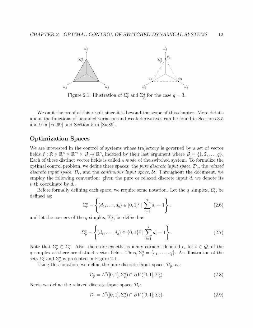
Σqr
d1
d2 d3
Σqp
d1
d2 d3
e1
e3e2
Figure 2.1: Illustration of Σqr and Σq
p for the case q = 3.
We omit the proof of this result since it is beyond the scope of this chapter. More detailsabout the functions of bounded variation and weak derivatives can be found in Sections 3.5and 9 in [Fol99] and Section 5 in [Zie89].
Optimization Spaces
We are interested in the control of systems whose trajectory is governed by a set of vectorfields f : R× Rn × Rm ×Q → Rn, indexed by their last argument where Q = {1, 2, . . . , q}.Each of these distinct vector fields is called a mode of the switched system. To formalize theoptimal control problem, we define three spaces: the pure discrete input space, Dp, the relaxeddiscrete input space, Dr, and the continuous input space, U . Throughout the document, weemploy the following convention: given the pure or relaxed discrete input d, we denote itsi–th coordinate by di.
Before formally defining each space, we require some notation. Let the q–simplex, Σqr, be
defined as:
Σqr =
{(d1, . . . , dq) ∈ [0, 1]q |
q∑i=1
di = 1
}, (2.6)
and let the corners of the q-simplex, Σqp, be defined as:
Σqp =
{(d1, . . . , dq) ∈ {0, 1}q |
q∑i=1
di = 1
}. (2.7)
Note that Σqp ⊂ Σq
r. Also, there are exactly as many corners, denoted ei for i ∈ Q, of theq–simplex as there are distinct vector fields. Thus, Σq
p = {e1, . . . , eq}. An illustration of thesets Σq
r and Σqp is presented in Figure 2.1.
Using this notation, we define the pure discrete input space, Dp, as:
Dp = L2([0, 1],Σqp) ∩BV ([0, 1],Σq
p). (2.8)
Next, we define the relaxed discrete input space, Dr:
Dr = L2([0, 1],Σqr) ∩BV ([0, 1],Σq
r). (2.9)
CHAPTER 2. OPTIMAL CONTROL OF SWITCHED DYNAMICAL SYSTEMS 13
Notice that the discrete input at each instance in time can be written as the linear combina-tion of the corners of the simplex. Given this observation, we employ these corners to indexthe vector fields, i.e. for each i ∈ Q we write f(·, ·, ·, ei) for f(·, ·, ·, i). Finally, we define thecontinuous input space, U :
U = L2([0, 1], U) ∩BV ([0, 1], U), (2.10)
where U ⊂ Rm is a bounded, convex set.Let X = L∞([0, 1],Rm) × L∞([0, 1],Rq) be endowed with the following norm for each
ξ = (u, d) ∈ X :‖ξ‖X = ‖u‖L2 + ‖d‖L2 , (2.11)
where the L2–norm is as defined in Equation (2.1). We combine U and Dp to define our pureoptimization space, Xp = U × Dp, and we endow it with the same norm as X . Similarly, wecombine U and Dr to define our relaxed optimization space, Xr = U ×Dr, and endow it withthe X–norm too. Note that Xp ⊂ Xr ⊂ X .
Trajectories, Cost, Constraint, and the Optimal Control Problem
Given ξ = (u, d) ∈ Xr, for convenience throughout the chapter we let:
f(t, x(t), u(t), d(t)
)=
q∑i=1
di(t)f(t, x(t), u(t), ei
), (2.12)
where d(t) =∑q
i=1 di(t)ei. We employ the same convention when we consider the partialderivatives of f . Given x0 ∈ Rn, we say that a trajectory of the system corresponding toξ ∈ Xr is the solution to:
x(t) = f(t, x(t), u(t), d(t)), ∀t ∈ [0, 1], x(0) = x0, (2.13)
and denote it by x(ξ) : [0, 1] → Rn, where we suppress the dependence on x0 in x(ξ) sinceit is assumed given. To ensure the clarity of the ensuing analysis, it is useful to sometimesemphasize the dependence of x(ξ)(t) on ξ. Therefore, we define the flow of the system,ϕt : Xr → Rn for each t ∈ [0, 1] as:
ϕt(ξ) = x(ξ)(t). (2.14)
To define the cost function, we assume that we are given a terminal cost, h0 : Rn → R.The cost function, J : Xr → R, for the optimal control problem is then defined as:
J(ξ) = h0
(x(ξ)(1)
). (2.15)
Notice that if the problem formulation includes a running cost, then one can extend theexisting state vector by introducing a new state, and modifying the cost function to evaluate

CHAPTER 2. OPTIMAL CONTROL OF SWITCHED DYNAMICAL SYSTEMS 14
this new state at the final time, as shown in Section 4.1.2 in [Pol97]. By performing this typeof modification, observe that each mode of the switched system can have a different runningcost associated with it.
Next, we define a family of functions, hj : Rn → R for j ∈ J = {1, . . . , Nc}. Given aξ ∈ Xr, the state x(ξ) is said to satisfy the constraint if hj(x
(ξ)(t)) ≤ 0 for each t ∈ [0, 1]and for each j ∈ J . We compactly describe all the constraints by defining the constraintfunction Ψ : Xr → R, by:
Ψ(ξ) = maxj∈J , t∈[0,1]
hj(x(ξ)(t)
), (2.16)
since hj(x(ξ)(t)
)≤ 0 for each t and j if and only if ψ(ξ) ≤ 0. To ensure the clarity of the
ensuing analysis, it is useful to sometimes emphasize the dependence of hj(x(ξ)(t)
)on ξ.
Therefore, we define component constraint functions, ψj,t : Xr → R for each t ∈ [0, 1] andj ∈ J as:
ψj,t(ξ) = hj (ϕt(ξ)) . (2.17)
With these definitions, we can state the Switched System Optimal Control Problem:
(SSOCP) minξ∈Xp{J(ξ) | Ψ(ξ) ≤ 0} . (2.18)
Assumptions and Uniqueness
In order to devise an algorithm to solve Switched System Optimal Control Problem, we makethe following assumptions about the dynamics, cost, and constraints:
Assumption 2.2. For each i ∈ Q, f(·, ·, ·, ei) is differentiable in both x and u. Also, eachf(·, ·, ·, ei) and its partial derivatives are Lipschitz continuous with constant L > 0, i.e. givent1, t2 ∈ [0, 1], x1, x2 ∈ Rn, and u1, u2 ∈ U :
(1) ‖f(t1, x1, u1, ei)− f(t2, x2, u2, ei)‖2 ≤ L (|t1 − t2|+ ‖x1 − x2‖2 + ‖u1 − u2‖2),
(2)∥∥∂f∂x
(t1, x1, u1, ei)− ∂f∂x
(t2, x2, u2, ei)∥∥i,2≤ L (|t1 − t2|+ ‖x1 − x2‖2 + ‖u1 − u2‖2),
(3)∥∥∂f∂u
(t1, x1, u1, ei)− ∂f∂u
(t2, x2, u2, ei)∥∥i,2≤ L (|t1 − t2|+ ‖x1 − x2‖2 + ‖u1 − u2‖2).
Assumption 2.3. The functions h0 and hj are Lipschitz continuous and differentiable inx for all j ∈ J . In addition, the derivatives of these functions with respect to x are alsoLipschitz continuous with constant L > 0, i.e. given x1, x2 ∈ Rn, for each j ∈ J :
(1) |h0(x1)− h0(x2)| ≤ L ‖x1 − x2‖2,
(2)∥∥∂h0∂x
(x1)− ∂h0∂x
(x2)∥∥
2≤ L ‖x1 − x2‖2,
(3) |hj(x1)− hj(x2)| ≤ L ‖x1 − x2‖2,
(4)∥∥∥∂hj∂x (x1)− ∂hj
∂x(x2)
∥∥∥2≤ L ‖x1 − x2‖2.
CHAPTER 2. OPTIMAL CONTROL OF SWITCHED DYNAMICAL SYSTEMS 15
If a running cost is included in the problem statement (i.e. if the cost also depends on theintegral of a function), then this function must also satisfy Assumption 2.2. Assumption 2.3 isa standard assumption on the objectives and constraints and is used to prove the convergenceproperties of the algorithm defined in the next section. These assumptions lead to thefollowing result:
Lemma 2.4. There exists a constant C > 0 such that, for each ξ ∈ Xr and t ∈ [0, 1],∥∥x(ξ)(t)∥∥
2≤ C, (2.19)
where x(ξ) is a solution of Differential Equation (2.13).
Proof. Given ξ = (u, d) ∈ Xr and noticing that |di(t)| ≤ 1 for all i ∈ Q and t ∈ [0, 1], wehave: ∥∥x(ξ)(t)
∥∥2≤ ‖x0‖2 +
q∑i=1
∫ t
0
∥∥f(s, x(ξ)(s), u(s), ei)∥∥
2ds. (2.20)
Next, observe that ‖f(0, x0, 0, ei)‖2 is bounded for all i ∈ Q and u(s) is bounded for eachs ∈ [0, 1] since U is bounded. Then by Assumption 2.2, we know there exists a K > 0 suchthat for each s ∈ [0, 1], i ∈ Q, and ξ ∈ Xr,∥∥f(s, x(ξ)(s), u(s), ei
)∥∥2≤ K
(∥∥x(ξ)(s)∥∥
2+ 1). (2.21)
Applying the Bellman-Gronwall Inequality (Lemma 5.6.4 in [Pol97]) to Equation (2.20), wehave
∥∥x(ξ)(t)∥∥
2≤ eqK
(1 + ‖x0‖2
)for each t ∈ [0, 1]. Since x0 is assumed given and bounded,
we have our result.
In fact, this implies that the dynamics, cost, constraints, and their derivatives are allbounded:
Corollary 2.5. There exists a constant C > 0 such that for each ξ = (u, d) ∈ Xr, t ∈ [0, 1],and j ∈ J :
(1)∥∥f(t, x(ξ)(t), u(t), d(t)
)∥∥2≤ C,
∥∥∥∥∂f∂x(t, x(ξ)(t), u(t), d(t))∥∥∥∥
i,2
≤ C, and∥∥∥∥∂f∂u(t, x(ξ)(t), u(t), d(t))∥∥∥∥
i,2
≤ C.
(2)∣∣h0
(x(ξ)(t)
)∣∣ ≤ C, and
∥∥∥∥∂h0
∂x
(x(ξ)(t)
)∥∥∥∥2
≤ C.
(3)∣∣hj(x(ξ)(t)
)∣∣ ≤ C, and
∥∥∥∥∂hj∂x
(x(ξ)(t)
)∥∥∥∥2
≤ C.
Where x(ξ) is a solution of Differential Equation (2.13).

CHAPTER 2. OPTIMAL CONTROL OF SWITCHED DYNAMICAL SYSTEMS 16
Proof. The result follows immediately from the continuity of f , ∂f∂x
, ∂f∂u
, h0, ∂h0∂x
, hj, and∂hj∂x
for each j ∈ J , as stated in Assumptions 2.2 and 2.3, and the fact that each of the argumentsto these functions can be constrained to a compact domain, which follows from Lemma 2.4and the compactness of U and Σq
r.
An application of this corollary leads to a fundamental result:
Theorem 2.6. For each ξ ∈ Xr Differential Equation (2.13) has a unique solution.
Proof. First let us note that f , as defined in Equation (2.12), is also Lipschitz with respectto its fourth argument. Indeed, given t ∈ [0, 1], x ∈ Rn, u ∈ U , and d1, d2 ∈ Σq
r,
∥∥f(t, x, u, d1)− f(t, x, u, d2)∥∥
2=
∥∥∥∥∥q∑i=1
(d1,i − d2,i
)f(t, x, u, ei)
∥∥∥∥∥2
≤ Cq‖d1 − d2‖2,
(2.22)
where C > 0 is as in Corollary 2.5.Given that f is Lipschitz with respect to all its arguments, the result follows as a di-
rect extension of the classical existence and uniqueness theorem for nonlinear differentialequations (see Section 2.4.1 in [Vid02] for a standard version of this theorem).
Therefore, since x(ξ) is unique, it is not an abuse of notation to denote the solution ofDifferential Equation (2.13) by x(ξ). Next, we develop an algorithm to solve the SwitchedSystem Optimal Control Problem.
2.2 Optimization Algorithm
In this section, we describe our optimization algorithm. Our approach proceeds as follows:first, we treat a given pure discrete input as a relaxed discrete input by allowing it to belongDr; second, we perform optimal control over the relaxed optimization space; and finally, weproject the computed relaxed input into a pure input. Before describing our algorithm indetail, we begin with a brief digression to motivate why such a roundabout construction isrequired in order to devise a first order numerical optimal control scheme for the SwitchedSystem Optimal Control Problem defined in Equation (2.18).
Directional Derivatives
To appreciate why the construction of a numerical scheme to find the local minima of theSwitched System Optimal Control Problem defined in Equation (2.18) is difficult, supposethat the optimization in the problem took place over the relaxed optimization space rather

CHAPTER 2. OPTIMAL CONTROL OF SWITCHED DYNAMICAL SYSTEMS 17
than the pure optimization space. The Relaxed Switched System Optimal Control Problemis then defined as:
(RSSOCP) minξ∈Xr{J(ξ) | Ψ(ξ) ≤ 0} . (2.23)
The local minimizers of this problem are then defined as follows:
Definition 2.7. Let us denote an ε–ball in the X–norm centered at ξ by:
NX (ξ, ε) ={ξ ∈ Xr |
∥∥ξ − ξ∥∥X < ε}. (2.24)
We say that a point ξ ∈ Xr is a local minimizer of the Relaxed Switched System OptimalControl Problem defined in Equation (2.23) if Ψ(ξ) ≤ 0 and there exists ε > 0 such thatJ(ξ) ≥ J(ξ) for each ξ ∈ NX (ξ, ε) ∩
{ξ ∈ Xr | Ψ(ξ) ≤ 0
}.
Given this definition, a first order numerical optimal control scheme can exploit the vectorspace structure of the relaxed optimization space in order to define directional derivativesthat find local minimizers for this Relaxed Switched System Optimal Control Problem.
To concretize how such an algorithm would work, we introduce some additional notation.Given ξ ∈ Xr, Y a Euclidean space, and any function G : Xr → Y , the directional derivativeof G at ξ, denoted DG(ξ; ·) : X → Y , is computed as:
DG(ξ; ξ′) = limλ↓0
G(ξ + λξ′)−G(ξ)
λ. (2.25)
To understand the connection between directional derivatives and local minimizers, sup-pose the Relaxed Switched System Optimal Control Problem is unconstrained and considerthe first order approximation of the cost J at a point ξ ∈ Xr in the ξ′ ∈ X direction byemploying the directional derivative DJ(ξ; ξ′):
J(ξ + λξ′) ≈ J(ξ) + λDJ(ξ; ξ′), (2.26)
where 0 ≤ λ � 1. It follows that if DJ(ξ; ξ′), whose existence is proven in Lemma 2.24, isnegative, then it is possible to decrease the cost by moving in the ξ′ direction. That is ifthe directional derivative of the cost at a point ξ is negative along a certain direction, thenfor each ε > 0 there exists a ξ ∈ NX (ξ, ε) such that J(ξ) < J(ξ). Therefore if DJ(ξ; ξ′)is negative, then ξ is not a local minimizer of the unconstrained Relaxed Switched SystemOptimal Control Problem.
Similarly, for the general Relaxed Switched System Optimal Control Problem, considerthe first order approximation of each of the component constraint functions, ψj,t for eachj ∈ J and t ∈ [0, 1] at a point ξ ∈ Xr in the ξ ∈ X direction by employing the directionalderivative Dψj,t(ξ; ξ
′):ψj,t(ξ + λξ′) ≈ ψj,t(ξ) + λDψj,t(ξ; ξ
′), (2.27)

CHAPTER 2. OPTIMAL CONTROL OF SWITCHED DYNAMICAL SYSTEMS 18
where 0 ≤ λ� 1. It follows that if Dψj,t(ξ; ξ′), whose existence is proven in Lemma 2.27, is
negative, then it is possible to decrease the infeasibility of ϕt(ξ) with respect to hj by movingin the ξ′ direction. That is if the directional derivatives of the cost and all of the componentconstraints for all t ∈ [0, 1] at a point ξ are negative along a certain direction and Ψ(ξ) = 0,then for each ε > 0 there exists a ξ ∈ {ξ ∈ Xr | Ψ(ξ) ≤ 0} ∩NX (ξ, ε) such that J(ξ) < J(ξ).Therefore, if Ψ(ξ) = 0 and DJ(ξ; ξ′) and Dψj,t(ξ; ξ
′) are negative for all j ∈ J and t ∈ [0, 1],then ξ is not a local minimizer of the Relaxed Hybrid Optimal Control Problem. Similarly,if Ψ(ξ) < 0 and DJ(ξ; ξ′) is negative, then ξ is not a local minimizer of the Relaxed HybridOptimal Control Problem, even if Dψj,t(ξ; ξ
′) is greater than zero for all j ∈ J and t ∈ [0, 1].Returning to the Switched System Optimal Control Problem, it is unclear how to define
a directional derivative for the pure discrete input space since it is not a vector space.Therefore, in contrast to the relaxed discrete and continuous input spaces, the constructionof a first order numerical scheme for the optimization of the pure discrete input is non-trivial.One could imagine trying to exploit the directional derivatives in the relaxed optimizationspace in order to construct a first order numerical optimal control algorithm for the SwitchedSystem Optimal Control Problem, but this would require devising some type of connectionbetween points belonging to the pure and relaxed optimization spaces.
The Weak Topology on the Optimization Space and LocalMinimizers
To motivate the type of relationship required between the pure and relaxed optimizationspace in order to construct a first order numerical optimal control scheme, we begin bydescribing the Chattering Lemma:
Theorem 2.8 (Theorem 1 in [BD05]). For each ξr ∈ Xr and ε > 0 there exists a ξp ∈ Xpsuch that for each t ∈ [0, 1]:
‖ϕt(ξr)− ϕt(ξp)‖2 ≤ ε, (2.28)
where ϕt(ξr) and ϕt(ξp) are solutions to Differential Equation (2.13) corresponding to ξr andξp, respectively.
The theorem as is proven in [Ber74] is not immediately applicable to switched systems, buta straightforward extension as is proven in Theorem 1 in [BD05] makes that feasible. Notethat the theorem as stated in [BD05], considers only two vector fields (i.e. q = 2), but asthe author’s of the theorem remark, their proof can be generalized to an arbitrary numberof vector fields. A particular version of this existence theorem can also be found in Lemma 1in [Sus72].
Theorem 2.8 says that the behavior of any element of the relaxed optimization space withrespect to the trajectory of switched system can be approximated arbitrarily well by a pointin the pure optimization space. Unfortunately, the relaxed and pure point as in Theorem 2.8need not be near one another in the metric induced by the X -norm. Therefore, though thereexists a relationship between the pure and relaxed optimization spaces, this connection is

CHAPTER 2. OPTIMAL CONTROL OF SWITCHED DYNAMICAL SYSTEMS 19
not reflected in the topology induced by the X -norm; however, in a particular topology overthe relaxed optimization space, a relaxed point and the pure point that approximates it asin Theorem 2.8 can be made arbitrarily close:
Definition 2.9. We define the weak topology on Xr induced by Differential Equation (2.13)as the smallest topology on Xr such that the map ξ 7→ x(ξ) is continuous. Moreover, an ε-ballin the weak topology centered at ξ is denoted by:
Nw(ξ, ε) ={ξ ∈ Xr |
∥∥x(ξ) − x(ξ)∥∥L2 < ε
}. (2.29)
A longer introduction to weak topology can be found in Section 3.8 in [Rud91] or Sec-tion 2.3 in [KZ05], but before continuing we make an important observation that aids inmotivating the ensuing analysis. In order to understand the relationship between the topol-ogy generated by the X -norm on Xr and the weak topology on Xr, observe that ϕt is Lipschitzcontinuous for all t ∈ [0, 1] (this is proven in Corollary 2.13). Therefore, for any ε > 0 thereexists a δ > 0 such that if a pair of points of the relaxed optimization space belong to thesame δ–ball in the X–norm, then the pair of points belong to the same ε–ball in the weaktopology on Xr.
Notice, however, that it is not possible to show that for every ε > 0 that there existsa δ > 0 such that if a pair of points of the relaxed optimization space belong to the sameδ–ball in the weak topology on Xr, then the pair of points belong to the same ε–ball inthe X–norm. More informally, a pair of points may generate trajectories that are near oneanother in the L2–norm while not being near one another in the X–norm. Since the weaktopology, in contrast to the X–norm induced topology, naturally places points that generatenearby trajectories next to one another, we extend Definition 2.9 in order to define a weaktopology on Xp which we then use to define a notion of local minimizer for the SwitchedSystem Optimal Control Problem:
Definition 2.10. We say that a point ξ ∈ Xp is a local minimizers of the Switched SystemOptimal Control Problem defined in Equation (2.18) if Ψ(ξ) ≤ 0 and there exists ε > 0 suchthat J(ξ) ≥ J(ξ) for each ξ ∈ Nw(ξ, ε) ∩
{ξ ∈ Xp | Ψ(ξ) ≤ 0
}, where Nw is as defined in
Equation (2.29).
With this definition of local minimizer, we can exploit Theorem 2.8, even just as anexistence result, along with the notion of directional derivative over the relaxed optimizationspace to construct a necessary condition for optimality for the Switched System OptimalControl Problem.
An Optimality Condition
Motivated by the approach undertaken in [Pol97], we define an optimality function, denotedby θ : Xp → (−∞, 0], that determines whether a given point is a local minimizer of the

CHAPTER 2. OPTIMAL CONTROL OF SWITCHED DYNAMICAL SYSTEMS 20
Switched System Optimal Control Problem and a corresponding descent direction, g : Xp →Xr:
θ(ξ) = minξ′∈Xr
ζ(ξ, ξ′), g(ξ) = arg minξ′∈Xr
ζ(ξ, ξ′), (2.30)
where
ζ(ξ, ξ′) =
max
DJ(ξ; ξ′ − ξ), maxj∈Jt∈[0,1]
Dψj,t(ξ; ξ′ − ξ) + γΨ(ξ)
+ ‖ξ′ − ξ‖X if Ψ(ξ) ≤ 0,
max
DJ(ξ; ξ′ − ξ)−Ψ(ξ), maxj∈Jt∈[0,1]
Dψj,t(ξ; ξ′ − ξ)
+ ‖ξ′ − ξ‖X if Ψ(ξ) > 0,
(2.31)where γ > 0 is a design parameters. For notational convenience in the previous equationwe have left out the natural inclusion of ξ from Xp to Xr. Before proceeding, we make twoobservations. First, note that θ(ξ) ≤ 0 for each ξ ∈ Xp, since we can always choose ξ′ = ξwhich leaves the trajectory unmodified. Second, note that at a point ξ ∈ Xp the directionalderivatives in the optimality function consider directions ξ′−ξ with ξ′ ∈ Xr in order to ensurethat first order approximations constructed as in Equations (2.26) and (2.27) belong to therelaxed optimization space Xr which is convex (e.g. for 0 < λ� 1, J(ξ) + λDJ(ξ; ξ′ − ξ) ≈J((1− λ)ξ + λξ′) where (1− λ)ξ + λξ′ ∈ Xr).
To understand how the optimality function behaves, consider several cases. First, ifθ(ξ) < 0 and Ψ(ξ) = 0, then there exists a ξ′ ∈ Xr such that both DJ(ξ; ξ′ − ξ) andDψj,t(ξ; ξ
′−ξ) are negative for all j ∈ J and t ∈ [0, 1]. By employing the aforementioned firstorder approximation, we can show that for each ε > 0 there exists an ε–ball in the X -normcentered at ξ such that J(ξ) < J(ξ) for some ξ ∈ {ξ ∈ Xr | Ψ(ξ) ≤ 0}∩NX (ξ, ε). As a resultand because the cost and each of the component constraint functions are assumed Lipschitzcontinuous and ϕt for all t ∈ [0, 1] is Lipschitz continuous as is proven in Corollary 2.13,an application of Theorem 2.8 allows us to show that for each ε > 0 there exists an ε–ballin the weak topology on Xp centered at ξ such that J(ξp) < J(ξ) for some ξp ∈ {ξ ∈ Xp |Ψ(ξ) ≤ 0} ∩ Nw(ξ, ε). Therefore, it follows that if θ(ξ) < 0 and Ψ(ξ) = 0, then ξ is not alocal minimizer of the Switched System Optimal Control Problem.
Second, if θ(ξ) < 0 and Ψ(ξ) < 0, then there exists a ξ′ ∈ Xr such that DJ(ξ; ξ′ − ξ) isnegative. Though Dψj,t(ξ; ξ
′− ξ) maybe positive for some j ∈ J and t ∈ [0, 1], by employingthe aforementioned first order approximation, we can show that for each ε > 0 there existsan ε–ball in the X -norm centered at ξ such that J(ξ) < J(ξ) for some ξ ∈ {ξ ∈ Xr | Ψ(ξ) ≤0} ∩ NX (ξ, ε). As a result and because the cost and each of the constraint functions areassumed Lipschitz continuous and ϕt for all t ∈ [0, 1] is Lipschitz continuous as is proven inCorollary 2.13, an application of Theorem 2.8 allows us to show that for each ε > 0 thereexists an ε–ball in the weak topology on Xp centered at ξ such that J(ξp) < J(ξ) for someξp ∈ {ξ ∈ Xp | Ψ(ξ) ≤ 0} ∩ Nw(ξ, ε). Therefore, it follows that if θ(ξ) < 0 and Ψ(ξ) < 0,then ξ is not a local minimizer of the Switched System Optimal Control Problem. In this

CHAPTER 2. OPTIMAL CONTROL OF SWITCHED DYNAMICAL SYSTEMS 21
case, the addition of the Ψ term in ζ ensures that a direction that reduces the cost does notsimultaneously require a decrease in the infeasibility in order to be considered as a potentialdescent direction.
Third, if θ(ξ) < 0 and Ψ(ξ) > 0, then there exists a ξ′ ∈ Xr such that Dψj,t(ξ; ξ′ −
ξ) is negative for all j ∈ J and t ∈ [0, 1]. By employing the aforementioned first orderapproximation, we can show for each ε > 0 there exists an ε–ball in the X -norm centeredat ξ such that Ψ(ξ) < Ψ(ξ) for some ξ ∈ NX (ξ, ε). As a result and because each of theconstraint functions are assumed Lipschitz continuous and ϕt for all t ∈ [0, 1] is Lipschitzcontinuous as is proven in Corollary 2.13, an application of Theorem 2.8 allows us to showthat for each ε > 0 there exists an ε–ball in the weak topology on Xp centered at ξ suchthat Ψ(ξp) < Ψ(ξ) for some ξp ∈ Nw(ξ, ε). Therefore, though it is clear that ξ is not a localminimizer of the Switched System Optimal Control Problem since Ψ(ξ) > 0, it follows thatif θ(ξ) < 0 and Ψ(ξ) > 0, then it is possible to locally reduce the infeasibility of ξ. In thiscase, the addition of the DJ term in ζ serves as a heuristic to ensure that the reduction ininfeasibility does not come at the price of an undue increase in the cost.
These observations are formalized in Theorem 2.34 where we prove that if ξ is a localminimizer of the Switched System Optimal Control Problem, then θ(ξ) = 0, or that θ(ξ) = 0is a necessary condition for the optimality of ξ. To illustrate the importance of θ satisfyingthis property, recall how the directional derivative of a cost function is employed duringunconstrained finite dimensional optimization. Since the directional derivative of the costfunction at a point being equal to zero in all directions is a necessary condition for optimal-ity for an unconstrained finite dimensional optimization problem, it is used as a stoppingcriterion by first order numerical algorithms (Corollary 1.1.3 and Algorithm Model 1.2.23in [Pol97]). Similarly, by satisfying Theorem 2.34, θ is a necessary condition for optimalityfor the Switched System Optimal Control Problem and can therefore be used as a stoppingcriterion for a first order numerical optimal control algorithm trying to solve the SwitchedSystem Optimal Control Problem. Given θ’s importance, we say a point, ξ ∈ Xp, satisfiesthe optimality condition if θ(ξ) = 0.
Choosing a Step Size and Projecting the Relaxed Discrete Input
Impressively, Theorem 2.8 just as an existence result is sufficient to allow for the constructionof an optimality function that encapsulates a necessary condition for optimality for the Swit-ched System Optimal Control Problem. Unfortunately, Theorem 2.8 is unable to describehow to exploit the descent direction, g(ξ), since its proof provides no means to construct apure input that approximates the behavior of a relaxed input while controlling the qualityof the approximation. In this chapter, we extend Theorem 2.8 by devising a scheme thatremedies this shortcoming. This allows for the development of a numerical optimal controlalgorithm for the Switched System Optimal Control Problem that first, performs optimalcontrol over the relaxed optimization space and then projects the computed relaxed controlinto a pure control.

CHAPTER 2. OPTIMAL CONTROL OF SWITCHED DYNAMICAL SYSTEMS 22
Before describing the construction of this projection, we describe how the descent direc-tion, g(ξ), can be exploited to construct a point in the relaxed optimization space that eitherreduces the cost (if the ξ is feasible) or the infeasibility (if ξ is infeasible). Comparing ourapproach to finite dimensional optimization, the argument that minimizes ζ is a “direction”along which to move the inputs in order to reduce the cost in the relaxed optimization space,but we require an algorithm to choose a step size. We employ a line search algorithm similarto the traditional Armijo algorithm used during finite dimensional optimization in order tochoose a step size (Algorithm Model 1.2.23 in [Pol97]). Fixing α ∈ (0, 1) and β ∈ (0, 1), astep size for a point ξ ∈ Xp is chosen by solving the following optimization problem:
µ(ξ) =
min
{k ∈ N | J
(ξ + βk(g(ξ)− ξ)
)− J(ξ) ≤ αβkθ(ξ),
Ψ(ξ + βk(g(ξ)− ξ)
)≤ αβkθ(ξ)
}if Ψ(ξ) ≤ 0,
min{k ∈ N | Ψ
(ξ + βk(g(ξ)− ξ)
)−Ψ(ξ) ≤ αβkθ(ξ)
}if Ψ(ξ) > 0.
(2.32)
In Lemma 2.43, we prove that for ξ ∈ Xp, if θ(ξ) < 0, then µ(ξ) <∞. Therefore, if θ(ξ) < 0for some ξ ∈ Xp, then we can construct a descent direction, g(ξ), and a step size, µ(ξ), anda new point
(ξ + βµ(ξ)(g(ξ)− ξ)
)∈ Xr that produces a reduction in the cost (if ξ is feasible)
or a reduction in the infeasibility (if ξ is infeasible).We define the projection that takes this constructed point to a point belonging the
pure optimization space while controlling the quality of approximation in two steps. First,we approximate the relaxed input by its N–th partial sum approximation via the Haarwavelet basis. To define this operation, FN : L2([0, 1],R) ∩ BV ([0, 1],R) → L2([0, 1],R) ∩BV ([0, 1],R), we employ the Haar wavelet (Section 7.2.2 in [Mal99]):
λ(t) =
1 if t ∈
[0, 1
2
),
−1 if t ∈[
12, 1),
0 otherwise.
(2.33)
Letting 1 : R → R be the constant function equal to one and bkj : [0, 1] → R for k ∈ Nand j ∈ {0, . . . , 2k − 1}, be defined as bkj(t) = λ
(2kt − j
), the projection FN for some
c ∈ L2([0, 1],R) ∩BV ([0, 1],R)→ L2([0, 1],R) ∩BV ([0, 1],R) is defined as:
[FN(c)](t) = 〈c,1〉+N∑k=0
2k−1∑j=0
〈c, bkj〉bkj(t)
‖bkj‖2L2
. (2.34)
Note that the inner product here is the traditional Hilbert space inner product.This projection is then applied to each of the coordinates of an element in the relaxed
optimization space. To avoid introducing additional notation, we let the coordinate-wiseapplication of FN to some relaxed discrete input d ∈ Dr be denoted as FN(d) and similarlyfor some continuous input u ∈ U . Lemma 2.35 proves that for each N ∈ N, each t ∈ [0, 1],
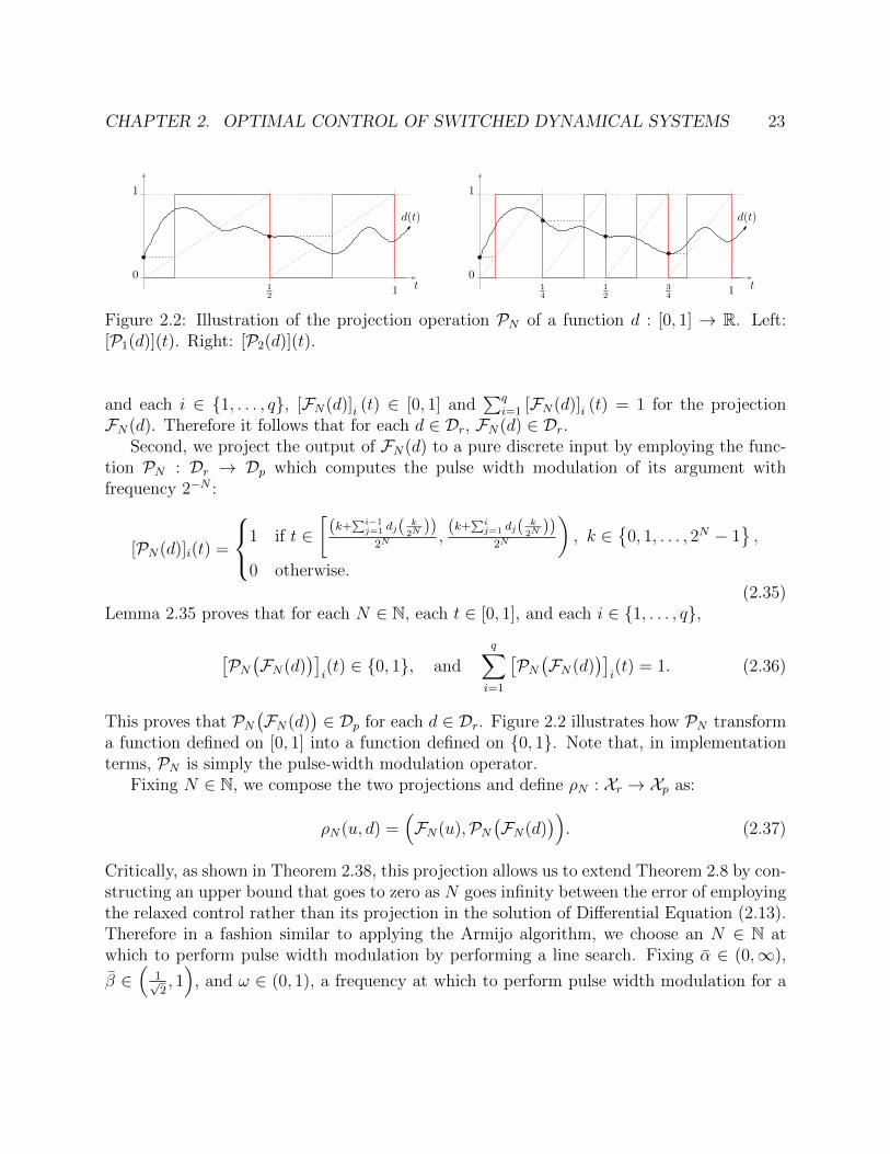
CHAPTER 2. OPTIMAL CONTROL OF SWITCHED DYNAMICAL SYSTEMS 23
d(t)
t
1
012 1 t
1
014
12
34 1
d(t)
Figure 2.2: Illustration of the projection operation PN of a function d : [0, 1] → R. Left:[P1(d)](t). Right: [P2(d)](t).
and each i ∈ {1, . . . , q}, [FN(d)]i (t) ∈ [0, 1] and∑q
i=1 [FN(d)]i (t) = 1 for the projectionFN(d). Therefore it follows that for each d ∈ Dr, FN(d) ∈ Dr.
Second, we project the output of FN(d) to a pure discrete input by employing the func-tion PN : Dr → Dp which computes the pulse width modulation of its argument withfrequency 2−N :
[PN(d)]i(t) =
1 if t ∈[
(k+∑i−1j=1 dj( k
2N))
2N,(k+
∑ij=1 dj( k
2N))
2N
), k ∈
{0, 1, . . . , 2N − 1
},
0 otherwise.
(2.35)Lemma 2.35 proves that for each N ∈ N, each t ∈ [0, 1], and each i ∈ {1, . . . , q},
[PN(FN(d)
)]i(t) ∈ {0, 1}, and
q∑i=1
[PN(FN(d)
)]i(t) = 1. (2.36)
This proves that PN(FN(d)
)∈ Dp for each d ∈ Dr. Figure 2.2 illustrates how PN transform
a function defined on [0, 1] into a function defined on {0, 1}. Note that, in implementationterms, PN is simply the pulse-width modulation operator.
Fixing N ∈ N, we compose the two projections and define ρN : Xr → Xp as:
ρN(u, d) =(FN(u),PN
(FN(d)
)). (2.37)
Critically, as shown in Theorem 2.38, this projection allows us to extend Theorem 2.8 by con-structing an upper bound that goes to zero as N goes infinity between the error of employingthe relaxed control rather than its projection in the solution of Differential Equation (2.13).Therefore in a fashion similar to applying the Armijo algorithm, we choose an N ∈ N atwhich to perform pulse width modulation by performing a line search. Fixing α ∈ (0,∞),
β ∈(
1√2, 1)
, and ω ∈ (0, 1), a frequency at which to perform pulse width modulation for a

CHAPTER 2. OPTIMAL CONTROL OF SWITCHED DYNAMICAL SYSTEMS 24
point ξ ∈ Xp is computed by solving the following optimization problem:
ν(ξ) =
min{k ∈ N | ξ′ = ρk
(ξ + βµ(ξ)(g(ξ)− ξ)
),
J(ξ′)− J(ξ) ≤(αβµ(ξ) − αβk
)θ(ξ), Ψ(ξ′) ≤ 0,
αβk ≤ (1− ω)αβµ(ξ)}
if Ψ(ξ) ≤ 0,
min{k ∈ N | ξ′ = ρk
(ξ + βµ(ξ)(g(ξ)− ξ)
),
Ψ(ξ′)−Ψ(ξ) ≤(αβµ(ξ) − αβk
)θ(ξ),
αβk ≤ (1− ω)αβµ(ξ)}
if Ψ(ξ) > 0.
(2.38)
In Lemma 2.44, we prove that for ξ ∈ Xp, if θ(ξ) < 0, then ν(ξ) < ∞. Therefore, ifθ(ξ) < 0 for some ξ ∈ Xp, then we can construct a descent direction, g(ξ), a step size,µ(ξ), a frequency at which to perform pulse width modulation, ν (ξ), and a new pointρν(ξ)
(ξ + βµ(ξ)(g(ξ) − ξ)
)∈ Xp that produces a reduction in the cost (if ξ is feasible) or a
reduction in the infeasibility (if ξ is infeasible).
Switched System Optimal Control Algorithm
Consolidating our definitions, Algorithm 2.1 describes our numerical method to solve theSwitched System Optimal Control Problem. For analysis purposes, we define Γ : Xp → Xpby
Γ(ξ) = ρν(ξ)
(ξ + βµ(ξ)(g(ξ)− ξ)
). (2.39)
We say {ξj}j∈N is a sequence generated by Algorithm 2.1 if ξj+1 = Γ(ξj) for each j ∈ N. Wecan prove several important properties about the sequence generated by Algorithm 2.1. First,in Lemma 2.45, we prove that if there exists i0 ∈ N such that Ψ(ξi0) ≤ 0, then Ψ(ξi) ≤ 0 foreach i ≥ i0. That is, if the Algorithm constructs a feasible point, then the sequence of pointsgenerated after this feasible point are always feasible. Second, in Theorem 2.46, we provelimj→∞ θ(ξj) = 0 or that Algorithm 2.1 converges to a point that satisfies the optimalitycondition.
2.3 Algorithm Analysis
In this section, we derive the various components of Algorithm 2.1 and prove that Algo-rithm 2.1 converges to a point that satisfies our optimality condition. Our argument pro-ceeds as follows: first, we prove the continuity of the state, cost, and constraint, which weemploy in latter arguments; second, we construct the components of the optimality functionand prove that these components satisfy various desired properties; third, we prove that wecan control the quality of approximation between the trajectories generated by a relaxeddiscrete input and its projection by ρN as a function of N ; finally, we prove the convergenceof our algorithm.
CHAPTER 2. OPTIMAL CONTROL OF SWITCHED DYNAMICAL SYSTEMS 25
Require: ξ0 ∈ Xp, α ∈ (0, 1), α ∈ (0,∞), β ∈ (0, 1), β ∈(
1√2, 1)
, γ ∈ (0,∞), ω ∈ (0, 1).
1: Set j = 0.2: loop3: Compute θ(ξj) as defined in Equation (2.30).4: if θ(ξj) = 0 then5: return ξj.6: end if7: Compute g(ξj) as defined in Equation (2.30).8: Compute µ(ξj) as defined in Equation (2.32).9: Compute ν(ξj) as defined in Equation (2.38).
10: Set ξj+1 = ρν(ξj)
(ξj + βµ(ξj)(g(ξj)− ξj)
), as defined in Equation (2.37).
11: Replace j by j + 1.12: end loop
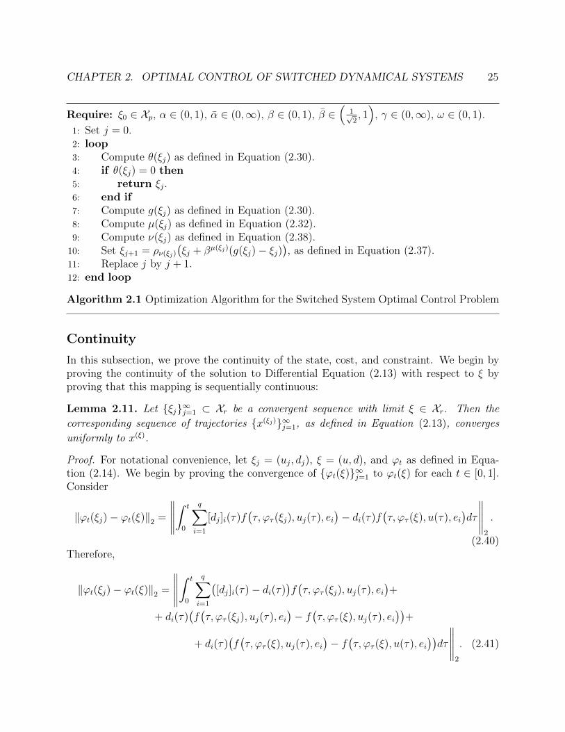
Algorithm 2.1 Optimization Algorithm for the Switched System Optimal Control Problem
Continuity
In this subsection, we prove the continuity of the state, cost, and constraint. We begin byproving the continuity of the solution to Differential Equation (2.13) with respect to ξ byproving that this mapping is sequentially continuous:
Lemma 2.11. Let {ξj}∞j=1 ⊂ Xr be a convergent sequence with limit ξ ∈ Xr. Then the
corresponding sequence of trajectories {x(ξj)}∞j=1, as defined in Equation (2.13), converges
uniformly to x(ξ).
Proof. For notational convenience, let ξj = (uj, dj), ξ = (u, d), and ϕt as defined in Equa-tion (2.14). We begin by proving the convergence of {ϕt(ξ)}∞j=1 to ϕt(ξ) for each t ∈ [0, 1].Consider
‖ϕt(ξj)− ϕt(ξ)‖2 =
∥∥∥∥∥∫ t
0
q∑i=1
[dj]i(τ)f(τ, ϕτ (ξj), uj(τ), ei
)− di(τ)f
(τ, ϕτ (ξ), u(τ), ei
)dτ
∥∥∥∥∥2
.
(2.40)Therefore,
‖ϕt(ξj)− ϕt(ξ)‖2 =
∥∥∥∥∥∫ t
0
q∑i=1
([dj]i(τ)− di(τ)
)f(τ, ϕτ (ξj), uj(τ), ei
)+
+ di(τ)(f(τ, ϕτ (ξj), uj(τ), ei
)− f
(τ, ϕτ (ξ), uj(τ), ei
))+
+ di(τ)(f(τ, ϕτ (ξ), uj(τ), ei
)− f
(τ, ϕτ (ξ), u(τ), ei
))dτ
∥∥∥∥∥2
. (2.41)

CHAPTER 2. OPTIMAL CONTROL OF SWITCHED DYNAMICAL SYSTEMS 26
Applying the Triangle Inequality, Assumption 2.2, Condition 1 in Corollary 2.5, and theboundedness of d, we have that there exists a C > 0 such that
‖ϕt(ξj)− ϕt(ξ)‖2 ≤∫ 1
0
q∑i=1
C∣∣[dj]i(τ)− di(τ)
∣∣+L ‖ϕτ (ξj)− ϕτ (ξ)‖2 +L ‖uj(τ)− u(τ)‖2 dτ.
(2.42)Applying the Bellman-Gronwall Inequality (Lemma 5.6.4 in [Pol97]), we have that
‖ϕt(ξj)− ϕt(ξ)‖2 ≤ eL(∫ 1
0
C ‖dj(τ)− d(τ)‖1 + L ‖uj(τ)− u(τ)‖2 dτ
). (2.43)
Note that ‖u‖2 ≤ ‖u‖1 for each u ∈ Rm. Then applying Holder’s inequality (Proposition 6.2in [Fol99]) to the vector valued function, we have:∫ 1
0
‖dj(τ)− d(τ)‖1 dτ ≤ ‖dj − d‖L2 , and
∫ 1
0
‖uj(τ)− u(τ)‖1 dτ ≤ ‖uj − u‖L2 . (2.44)
Since the sequence ξj converges to ξ, for every ε > 0 we know there exists some j0 suchthat for all j greater than j0, ‖ξj − ξ‖X ≤ ε. Therefore ‖ϕt(ξj) − ϕt(ξ)‖2 ≤ eL(L + C)ε,which proves the convergence of {ϕt(ξj)}∞j=1 to ϕt(ξ) for each t ∈ [0, 1] as j →∞. Since this
bound does not depend on t, we in fact have the uniform convergence of {x(ξj)}∞j=1 to x(ξ) asj →∞, hence obtaining our desired result.
Notice that since Xr is a metric space, the previous result proves that the function ϕtwhich assigns ξ ∈ Xr to ϕt(ξ) as the solution of Differential Equation (2.13) employing thenotation defined in Equation (2.14) is continuous.
Corollary 2.12. The function ϕt that maps ξ ∈ Xr to ϕt(ξ) as the solution of DifferentialEquation (2.13) where we employ the notation defined in Equation (2.14) is continuous forall t ∈ [0, 1].
In fact, our arguments have shown that this mapping is Lipschitz continuous:
Corollary 2.13. There exists a constant L > 0 such that for each ξ1, ξ2 ∈ Xr and t ∈ [0, 1]:
‖ϕt(ξ1)− ϕt(ξ2)‖2 ≤ L‖ξ1 − ξ2‖X , (2.45)
where ϕt(ξ) is as defined in Equation (2.14).
As a result of this corollary, we immediately have the following results:
Corollary 2.14. There exists a constant L > 0 such that for each ξ1 = (u1, d1) ∈ Xr,ξ2 = (u2, d2) ∈ Xr, and t ∈ [0, 1]:
(1)∥∥f(t, ϕt(ξ1), u1(t), d1(t)
)−f(t, ϕt(ξ2), u2(t), d2(t)
)∥∥2≤
≤ L(‖ξ1 − ξ2‖X + ‖u1(t)− u2(t)‖2 + ‖d1(t)− d2(t)‖2
),

CHAPTER 2. OPTIMAL CONTROL OF SWITCHED DYNAMICAL SYSTEMS 27
(2)
∥∥∥∥∂f∂x(t, ϕt(ξ1), u1(t), d1(t))−∂f∂x
(t, ϕt(ξ2), u2(t), d2(t)
)∥∥∥∥i,2
≤
≤ L(‖ξ1 − ξ2‖X + ‖u1(t)− u2(t)‖2 + ‖d1(t)− d2(t)‖2
),
(3)
∥∥∥∥∂f∂u(t, ϕt(ξ1), u1(t), d1(t))−∂f∂u
(t, ϕt(ξ2), u2(t), d2(t)
)∥∥∥∥i,2
≤
≤ L(‖ξ1 − ξ2‖X + ‖u1(t)− u2(t)‖2 + ‖d1(t)− d2(t)‖2
),
where ϕt(ξ) is as defined in Equation (2.14).
Proof. The proof of Condition 1 follows by the fact that the vector field f is Lipschitz inall its arguments, as shown in the proof of Theorem 2.6, and applying Corollary 2.13. Theremaining conditions follow in a similar fashion.
Corollary 2.15. There exists a constant L > 0 such that for each ξ1, ξ2 ∈ Xr, j ∈ J , andt ∈ [0, 1]:
(1)∣∣h0
(ϕ1(ξ1)
)− h0
(ϕ1(ξ2)
)∣∣ ≤ L ‖ξ1 − ξ2‖X ,
(2)∥∥∥∂h0∂x
(ϕ1(ξ1)
)− ∂h0
∂x
(ϕ1(ξ2)
)∥∥∥2≤ L ‖ξ1 − ξ2‖X ,
(3)∣∣hj(ϕt(ξ1)
)− hj
(ϕt(ξ2)
)∣∣ ≤ L ‖ξ1 − ξ2‖X ,
(4)∥∥∥∂hj∂x (ϕt(ξ1)
)− ∂hj
∂x
(ϕt(ξ2)
)∥∥∥2≤ L ‖ξ1 − ξ2‖X ,
where ϕt(ξ) is as defined in Equation (2.14).
Proof. This result follows by Assumption 2.3 and Corollary 2.13.
Even though it is a straightforward consequence of Condition 1 in Corollary 2.15, wewrite the following result to stress its importance.
Corollary 2.16. There exists a constant L > 0 such that, for each ξ1, ξ2 ∈ Xr:
|J(ξ1)− J(ξ2)| ≤ L ‖ξ1 − ξ2‖X (2.46)
where J is as defined in Equation (2.15).
In fact, the Ψ is also Lipschitz continuous:
Lemma 2.17. There exists a constant L > 0 such that, for each ξ1, ξ2 ∈ Xr:
|Ψ(ξ1)−Ψ(ξ2)| ≤ L ‖ξ1 − ξ2‖X (2.47)
where Ψ is as defined in Equation (2.16).
CHAPTER 2. OPTIMAL CONTROL OF SWITCHED DYNAMICAL SYSTEMS 28
Proof. Since the maximum in Ψ is taken over J × [0, 1], which is compact, and the maps(j, t) 7→ ψj,t(ξ) are continuous for each ξ ∈ X , we know from Condition 3 in Corollary 2.15that there exists L > 0 such that,
Ψ(ξ1)−Ψ(ξ2) = max(j,t)∈J×[0,1]
ψj,t(ξ1)− max(j,t)∈J×[0,1]
ψj,t(ξ2)
≤ max(j,t)∈J×[0,1]
ψj,t(ξ1)− ψj,t(ξ2)
≤ L ‖ξ1 − ξ2‖X .
(2.48)
By reversing ξ1 and ξ2, and applying the same argument we get the desired result.
Derivation of Algorithm Terms
Next, we formally derive the components of the optimality function and prove that it isproperly defined. We begin by deriving the formal expression for the directional derivativeof the trajectory of the switched system.
Lemma 2.18. Let ξ = (u, d) ∈ Xr, ξ′ = (u′, d′) ∈ X , and let ϕt : Xr → Rn be as definedin Equation (2.14). Then the directional derivative of ϕt, as defined in Equation (2.25), isgiven by
Dϕt(ξ; ξ′) =
∫ t
0
Φ(ξ)(t, τ)
(∂f
∂u
(τ, ϕτ (ξ), u(τ), d(τ)
)u′(τ) +
q∑i=1
f(τ, ϕτ (ξ), u(τ), ei
)d′i(τ)
)dτ,
(2.49)where Φ(ξ)(t, τ) is the unique solution of the following matrix differential equation:
∂Φ
∂t(t, τ) =
∂f
∂x
(t, ϕt(ξ), u(t), d(t)
)Φ(t, τ), t ∈ [0, 1], Φ(τ, τ) = I. (2.50)
Proof. For notational convenience, let x(λ) = x(ξ+λξ′), u(λ) = u + λu′, and d(λ) = d + λd′.Then, if we define ∆x(λ) = x(λ) − x(ξ),
∆x(λ)(t) =
∫ t
0
f(τ, x(λ)(τ), u(λ)(τ), d(λ)(τ)
)− f
(τ, x(ξ)(t), u(τ), d(τ)
)dτ, (2.51)
thus,
∆x(λ)(t) =
∫ t
0
f(τ, x(λ)(τ), u(λ)(τ), d(λ)(τ)
)− f
(τ, x(λ)(t), u(λ)(τ), d(τ)
)dτ+
+
∫ t
0
f(τ, x(λ)(τ), u(λ)(τ), d(τ)
)− f
(τ, x(ξ)(t), u(λ)(τ), d(τ)
)dτ+
+
∫ t
0
f(τ, x(ξ)(τ), u(λ)(τ), d(τ)
)− f
(τ, x(ξ)(t), u(τ), d(τ)
)dτ, (2.52)
CHAPTER 2. OPTIMAL CONTROL OF SWITCHED DYNAMICAL SYSTEMS 29
and applying the Mean Value Theorem,
∆x(λ)(t) =
∫ t
0
λ
q∑i=1
d′i(τ)f(τ, x(λ)(τ), u(λ)(τ), ei
)+
+
∫ t
0
∂f
∂x
(τ, x(ξ)(τ) + νx(τ)∆x(λ)(τ), u(λ)(τ), d(τ)
)∆x(λ)(τ)+
+
∫ t
0
λ∂f
∂u
(τ, x(ξ)(τ), u(τ) + νu(τ)λu′(τ), d(τ)
)u′(τ)dt, (2.53)
where νu, νx : [0, t]→ [0, 1].Let z(t) be the unique solution of the following differential equation:
z(τ) =∂f
∂x
(τ, x(ξ)(τ), u(τ), d(τ)
)z(τ) +
∂f
∂u
(τ, x(ξ)(τ), u(τ), d(τ)
)u′(τ)+
+
q∑i=1
d′i(τ)f(τ, x(ξ)(τ), u(τ), ei
), τ ∈ [0, t], z(0) = 0. (2.54)
We want to show that limλ↓0
∥∥∥∆x(λ)(t)λ− z(t)
∥∥∥2
= 0. To prove this, consider the following
inequalities that follow from Condition 2 in Assumption 2.2:∥∥∥∥∫ t
0
∂f
∂x
(τ, x(ξ)(τ), u(τ), d(τ)
)z(τ)+
− ∂f
∂x
(τ, x(ξ)(τ) + νx(τ)∆x(λ)(τ), u(λ)(τ), d(τ)
)∆x(λ)(τ)
λdτ
∥∥∥∥2
≤
≤∫ t
0
∥∥∥∥∂f∂x∥∥∥∥L∞
∥∥∥∥z(τ)− ∆x(λ)(τ)
λ
∥∥∥∥2
dτ +
∫ t
0
L(∥∥νx(τ)∆x(λ)(τ)
∥∥2
+ λ ‖u′(τ)‖2
)‖z(t)‖2 dτ
≤ L
∫ t
0
∥∥∥∥z(τ)− ∆x(λ)(τ)
λ
∥∥∥∥2
dτ + L
∫ t
0
(∥∥∆x(λ)(τ)∥∥
2+ λ ‖u′(τ)‖2
)‖z(t)‖2 dτ,
(2.55)also from Condition 3 in Assumption 2.2:∥∥∥∥∫ t
0
(∂f
∂u
(τ, x(ξ)(τ), u(τ), d(τ)
)− ∂f
∂u
(τ, x(ξ)(τ), u(τ) + νu(τ)λu′(τ), d(τ)
))u′(τ)
∥∥∥∥2
≤
≤ L
∫ t
0
λ ‖νu(τ)u′(τ)‖2 ‖u′(τ)‖2 dτ ≤ L
∫ t
0
λ ‖u′(τ)‖22 dτ, (2.56)

CHAPTER 2. OPTIMAL CONTROL OF SWITCHED DYNAMICAL SYSTEMS 30
and from Condition 1 in Assumption 2.2:∥∥∥∥∥∫ t
0
q∑i=1
d′i(τ)(f(τ, x(ξ)(τ), u(τ), ei
)− f
(τ, x(λ)(τ), u(λ)(τ), ei
))dτ
∥∥∥∥∥2
≤
≤ L
∫ t
0
q∑i=1
d′i(τ)(∥∥∆x(λ)(τ)
∥∥2
+ λ ‖u′(τ)‖2
)dτ. (2.57)
Now, using the Bellman-Gronwall Inequality (Lemma 5.6.4 in [Pol97]) and the inequalitiesabove,∥∥∥∥∆x(λ)(t)
λ− z(t)
∥∥∥∥2
≤ eLtL
(∫ t
0
(∥∥∆x(λ)(τ)∥∥
2+ λ ‖u′(τ)‖2
)‖z(t)‖2 + λ ‖u′(τ)‖2
2 +
+
q∑i=1
d′i(τ)(∥∥∆x(λ)(τ)
∥∥2
+ λ ‖u′(τ)‖2
)dτ
), (2.58)
but note that every term in the integral above is bounded, and ∆x(λ)(τ) → 0 for eachτ ∈ [0, t] since x(λ) → x(ξ) uniformly as shown in Lemma 2.11, thus by the DominatedConvergence Theorem (Theorem 2.24 in [Fol99]) and by noting that Dϕt(ξ; ξ
′), as defined inEquation (2.49), is exactly the solution of Differential Equation (2.54) we get:
limλ↓0
∥∥∥∥∆x(λ)(t)
λ− z(t)
∥∥∥∥2
= limλ↓0
1
λ
∥∥x(ξ+λξ′)(t)− x(ξ)(t)−Dϕt(ξ;λξ′)∥∥
2= 0. (2.59)
The result of the Lemma then follows.
Next, we prove that Dϕt is bounded by proving that Φ(ξ) is bounded:
Corollary 2.19. There exists a constant C > 0 such that for each t, τ ∈ [0, 1] and ξ ∈ Xr:∥∥Φ(ξ)(t, τ)∥∥i,2≤ C, (2.60)
where Φ(ξ)(t, τ) is the solution to Differential Equation (2.50).
Proof. Notice that, since the induced matrix norm is submultiplicative,∥∥Φ(ξ)(t, τ)∥∥i,2
=
∥∥∥∥Φ(ξ)(t, τ) +
∫ t
τ
(∂f
∂x
(s, x(ξ)(s), u(s), d(s)
)Φ(ξ)(s, τ)
)ds
∥∥∥∥i,2
≤ 1 +
∫ t
τ
∥∥∥∥∂f∂x(s, x(ξ)(s), u(s), d(s))∥∥∥∥
i,2
∥∥Φ(ξ)(t, s)∥∥i,2ds
≤ eqC ,
(2.61)
where in the last step we employed Condition 1 from Corollary 2.5 with a constant C > 0and the Bellman-Gronwall Inequality.
CHAPTER 2. OPTIMAL CONTROL OF SWITCHED DYNAMICAL SYSTEMS 31
Corollary 2.20. There exists a constant C > 0 such that for all ξ ∈ Xr, ξ′ ∈ X , andt ∈ [0, 1]:
‖Dϕt(ξ; ξ′)‖2 ≤ C ‖ξ′‖X , (2.62)
where Dϕt is as defined in Equation (2.49).
Proof. This result follows by employing the Cauchy-Schwarz Inequality, Corollary 2.5 andCorollary 2.19.
In fact, we can actually prove the Lipschitz continuity of Φ(ξ):
Lemma 2.21. There exists a constant L > 0 such that for each ξ1, ξ2 ∈ Xr and eacht, τ ∈ [0, 1]: ∥∥Φ(ξ1)(t, τ)− Φ(ξ2)(t, τ)
∥∥i,2≤ L ‖ξ1 − ξ2‖X , (2.63)
where Φ(ξ) is the solution to Differential Equation (2.50).
Proof. Letting ξ1 = (u1, d1) ∈ Xr and ξ2 = (u2, d2) ∈ Xr and by applying the TriangleInequality and noticing the induced matrix norm is compatible, observe:∥∥Φ(ξ1)(t, τ)− Φ(ξ2)(t, τ)
∥∥i,2≤
≤∫ t
τ
(∥∥∥∥∂f∂x (s, x(ξ2)(s), u2(s), d2(s))∥∥∥∥
i,2
∥∥Φ(ξ1)(s, τ)− Φ(ξ2)(s, τ)∥∥i,2
)ds+
+
∫ t
τ
(∥∥∥∥∂f∂x (s, x(ξ1)(s), u1(s), d1(s))− ∂f
∂x
(s, x(ξ2)(s), u2(s), d2(s)
)∥∥∥∥i,2
∥∥Φ(ξ1)(s, τ)∥∥i,2
)ds.
(2.64)
By applying Condition 1 in Corollary 2.5, Condition 2 in Corollary 2.14, Corollary 2.19, thesame argument as in Equation (2.44), and the Bellman-Gronwall Inequality (Lemma 5.6.4in [Pol97]), our desired result follows.
A simple extension of our previous argument shows that for all t ∈ [0, 1], Dϕt(ξ; ·) isLipschitz continuous with respect to its point of evaluation, ξ.
Lemma 2.22. There exists a constant L > 0 such that for each ξ1, ξ2 ∈ Xr, ξ′ ∈ X , andt ∈ [0, 1]:
‖Dϕt(ξ1; ξ′)−Dϕt(ξ2; ξ′)‖2 ≤ L‖ξ1 − ξ2‖X ‖ξ′‖X (2.65)
where Dϕt is as defined in Equation (2.49).

CHAPTER 2. OPTIMAL CONTROL OF SWITCHED DYNAMICAL SYSTEMS 32
Proof. Let ξ1 = (u1, d1), ξ2 = (u2, d2), and ξ′ = (u′, d′). Then, by applying the TriangleInequality, and noticing that the induced matrix norm is compatible, observe:
‖Dϕt(ξ1; ξ′)−Dϕt(ξ2; ξ′)‖2 ≤
≤∫ t
0
(∥∥Φ(ξ1)(t, s)− Φ(ξ2)(t, s)∥∥i,2
∥∥∥∥∂f∂u(s, x(ξ1)(s), u1(s), d1(s))∥∥∥∥
i,2
+
+∥∥Φ(ξ2)(t, s)
∥∥i,2
∥∥∥∥∂f∂u(s, x(ξ1)(s), u1(s), d1(s))− ∂f
∂u
(s, x(ξ2)(s), u2(s), d2(s)
)∥∥∥∥i,2
)‖u′(s)‖2 ds+
+
∫ t
0
q∑i=1
(∥∥Φ(ξ1)(t, s)− Φ(ξ2)(t, s)∥∥i,2
∥∥f(s, x(ξ1)(s), u1(s), ei)∥∥
2+
+∥∥Φ(ξ2)(t, s)
∥∥i,2
∥∥f(s, x(ξ1)(s), u1(s), ei)− f
(s, x(ξ2)(s), u2(s), ei
)∥∥2
)‖d′(s)‖ ds. (2.66)
By applying Corollary 2.19, Condition 1 in Corollary 2.5, Lemma 2.21, Conditions 1 and 3 inCorollary 2.14, together with the boundedness of u′(s) and d′(s), and an argument identicalto the one used in Equation (2.44), our desired result follows.
Next, we prove that Dϕt is simultaneously continuous with respect to both of its argu-ments.
Lemma 2.23. For each t ∈ [0, 1], ξ ∈ Xr, and ξ′ ∈ X , the map (ξ, ξ′) 7→ Dϕt(ξ; ξ′), as
defined in Equation (2.49), is continuous.
Proof. To prove this result, we can employ an argument identical to the one used in theproof of Lemma 2.11. First, note that u(t) ∈ U for each t ∈ [0, 1]. Second, note that Φ(ξ),f , ∂f
∂x, and ∂f
∂uare bounded, as shown in Corollary 2.19 and Condition 1 in Corollary 2.5.
Third, recall that Φ(ξ), f , and ∂f∂u
are Lipschitz continuous, as proven in Lemma 2.21 andConditions 1 and 3 in Corollary 2.14, respectively. Finally, the result follows after using anargument identical to the one used in Equation (2.44).
We can now construct the directional derivative of the cost J and prove it is Lipschitzcontinuous.
Lemma 2.24. Let ξ ∈ Xr, ξ′ ∈ X , and J be as defined in Equation (2.15). Then thedirectional derivative of the cost J in the ξ′ direction is:
DJ(ξ; ξ′) =∂h0
∂x
(ϕ1(ξ)
)Dϕ1(ξ; ξ′). (2.67)
Proof. The result follows directly by the Chain Rule and Lemma 2.18.

CHAPTER 2. OPTIMAL CONTROL OF SWITCHED DYNAMICAL SYSTEMS 33
Corollary 2.25. There exists a constant L > 0 such that for each ξ1, ξ2 ∈ Xr and ξ′ ∈ X :
|DJ(ξ1; ξ′)−DJ(ξ2; ξ′)| ≤ L ‖ξ1 − ξ2‖X ‖ξ′‖X , (2.68)
where DJ is as defined in Equation (2.67).
Proof. Notice by the Triangle Inequality and the Cauchy-Schwartz Inequality:
|DJ(ξ1; ξ′)−DJ(ξ2; ξ′)| ≤∥∥∥∥∂h0
∂x
(ϕ1(ξ1)
)∥∥∥∥2
‖Dϕ1(ξ1; ξ′)−Dϕ1(ξ2; ξ′)‖2 +
+
∥∥∥∥∂h0
∂x
(ϕ1(ξ1)
)− ∂h0
∂x
(ϕ1(ξ2)
)∥∥∥∥2
‖Dϕ1(ξ2; ξ′)‖2 . (2.69)
The result then follows by applying Condition 2 in Corollary 2.5, Condition 2 in Corol-lary 2.15, Corollary 2.20, and Lemma 2.22.
Next, we prove that DJ is simultaneously continuous with respect to both of its argu-ments, which is a direct consequence of Lemma 2.23.
Corollary 2.26. For each ξ ∈ Xr and ξ′ ∈ X , the map (ξ, ξ′) 7→ DJ(ξ; ξ′), as defined inEquation (2.67), is continuous.
Next, we construct the directional derivative of each of the component constraint func-tions ψj,t and prove that each of the component constraints is Lipschitz continuous.
Lemma 2.27. Let ξ ∈ Xr, ξ′ ∈ X , and ψj,t defined as in Equation (2.17). Then for eachj ∈ J and t ∈ [0, 1], the directional derivative of ψj,t, denoted Dψj,t, is given by:
Dψj,t(ξ; ξ′) =
∂hj∂x
(ϕt(ξ)
)Dϕt(ξ; ξ
′). (2.70)
Proof. The result follows using the Chain Rule and Lemma 2.18.
Corollary 2.28. There exists a constant L > 0 such that for each ξ1, ξ2 ∈ Xr, ξ′ ∈ X , andt ∈ [0, 1]:
|Dψj,t(ξ1; ξ′)−Dψj,t(ξ2; ξ′)| ≤ L ‖ξ1 − ξ2‖X ‖ξ′‖X , (2.71)
where Dψj,t is as defined in Equation (2.70).
Proof. Notice by the Triangle Inequality and the Cauchy Schwartz Inequality:
|Dψj,t(ξ1; ξ′)−Dψj,t(ξ2; ξ′)| ≤∥∥∥∥∂hj∂x
(ϕt(ξ1)
)∥∥∥∥2
‖Dϕt(ξ1; ξ′)−Dϕt(ξ2; ξ′)‖2 +
+
∥∥∥∥∂hj∂x
(ϕt(ξ1)
)− ∂hj
∂x
(ϕt(ξ2)
)∥∥∥∥2
‖Dϕt(ξ2; ξ′)‖2 . (2.72)
The result then follows by applying Condition 3 in Corollary 2.5, Condition 4 in Corol-lary 2.15, Corollary 2.20, and Lemma 2.22.
CHAPTER 2. OPTIMAL CONTROL OF SWITCHED DYNAMICAL SYSTEMS 34
Next, we prove that Dψj,t is simultaneously continuous with respect to both of its argu-ments, which follows directly from Lemma 2.23:
Corollary 2.29. For each ξ ∈ Xr, ξ′ ∈ X , and t ∈ [0, 1], the map (ξ, ξ′) 7→ Dψj,t(ξ; ξ′), as
defined in Equation (2.70), is continuous.
Given these results, we can begin describing the properties satisfied by the optimalityfunction:
Lemma 2.30. Let ζ be defined as in Equation (2.31). Then there exists a constant L > 0such that, for each ξ1, ξ2, ξ
′ ∈ Xr,
|ζ(ξ1, ξ′)− ζ(ξ2, ξ
′)| ≤ L ‖ξ1 − ξ2‖X . (2.73)
Proof. To prove the result, first notice that for {xi}i∈I , {yi}i∈I ⊂ R:∣∣∣maxi∈I
xi
∣∣∣ ≤ maxi∈I|xi| , and max
i∈Ixi −max
i∈Iyi ≤ max
i∈I
{xi − yi
}. (2.74)
Therefore, ∣∣∣maxi∈I
xi −maxi∈I
yi
∣∣∣ ≤ maxi∈I|xi − yi|. (2.75)
Letting Ψ+(ξ) = max{0,Ψ(ξ)} and Ψ−(ξ) = max{0,−Ψ(ξ)}, observe:
ζ(ξ, ξ′) = max
{DJ(ξ; ξ′ − ξ)−Ψ+(ξ), max
j∈J , t∈[0,1]Dψj,t(ξ; ξ
′ − ξ)− γΨ−(ξ)
}+ ‖ξ′ − ξ‖X .
(2.76)Employing Equation (2.75):
∣∣ζ(ξ1, ξ′)− ζ(ξ2, ξ
′)∣∣ ≤ max
{∣∣DJ(ξ1; ξ′ − ξ1)−DJ(ξ2; ξ′ − ξ2)∣∣+∣∣Ψ+(ξ2)−Ψ+(ξ1)
∣∣,max
j∈J , t∈[0,1]
∣∣Dψj,t(ξ1; ξ′−ξ1)−Dψj,t(ξ2; ξ′−ξ2)∣∣+γ∣∣Ψ−(ξ2)−Ψ−(ξ1)
∣∣}+∣∣‖ξ′−ξ1‖X−‖ξ′−ξ2‖X
∣∣.(2.77)
We show three results that taken together with the Triangle Inequality prove the desiredresult. First, by applying the reverse Triangle Inequality:∣∣‖ξ′ − ξ1‖X − ‖ξ′ − ξ2‖X
∣∣ ≤ ‖ξ1 − ξ2‖X . (2.78)
Second,∣∣DJ(ξ1; ξ′ − ξ1)−DJ(ξ2; ξ′ − ξ2)∣∣ ≤ ∣∣DJ(ξ1; ξ′)−DJ(ξ2; ξ′)
∣∣+∣∣DJ(ξ1; ξ1)−DJ(ξ2; ξ1)
∣∣++
∣∣∣∣∂h0
∂x
(ϕ1(ξ2)
)Dϕ1(ξ2; ξ2 − ξ1)
∣∣∣∣≤ L ‖ξ1 − ξ2‖X ,
(2.79)

CHAPTER 2. OPTIMAL CONTROL OF SWITCHED DYNAMICAL SYSTEMS 35
where L > 0 and we employed the linearity of DJ , Corollary 2.25, the fact that ξ′ and ξ1
are bounded since ξ′, ξ1 ∈ Xr, the Cauchy-Schwartz Inequality, Condition 2 in Corollary 2.5,and Corollary 2.20. Notice that by employing an argument identical to Equation (2.79) andCorollary 2.28, we can assume without loss of generality that
∣∣Dψj,t(ξ1; ξ′−ξ1)−Dψj,t(ξ2; ξ′−ξ2)∣∣ ≤ L ‖ξ1 − ξ2‖X . Finally, notice that by applying Lemma 2.17, Ψ+(ξ) and Ψ−(ξ) are
Lipschitz continuous.
In fact, ζ satisfies an even more important property:
Lemma 2.31. For each ξ ∈ Xp, the map ξ′ 7→ ζ(ξ, ξ′), as defined in Equation (2.31), isstrictly convex.
Proof. The proof follows after noting that the maps ξ′ 7→ DJ(ξ; ξ′−ξ) and ξ′ 7→ Dψj,t(ξ; ξ′−ξ)
are affine, hence any maximum among these function is convex, and the map ξ′ 7→ ‖ξ′− ξ‖Xis strictly convex since we chose the 2–norm as our finite dimensional norm.
The following theorem, which follows as a result of the previous lemma, is fundamentalto our result since it shows that g, as defined in Equation (2.30), is a well-defined function.We omit the proof since it is a particular case of a well known result regarding the exis-tence of unique minimizers of strictly convex functions over bounded sets in Hilbert spaces(Proposition II.1.2 in [ET87]).
Theorem 2.32. For each ξ ∈ Xp, the map ξ′ 7→ ζ(ξ, ξ′), as defined in Equation (2.31), hasa unique minimizer.
Employing these results we can prove the continuity of the optimality function. Thisresult is not strictly required in order to prove the convergence of Algorithm 2.1 or in order toprove that the optimality function encodes local minimizers of the Switched System OptimalControl Problem, but is useful when we describe the implementation of our algorithm.
Lemma 2.33. The function θ, as defined in Equation (2.30), is continuous.
Proof. First, we show that θ is upper semi-continuous. Consider a sequence {ξi}∞i=1 ⊂ Xrconverging to ξ, and ξ′ ∈ Xr such that θ(ξ) = ζ(ξ, ξ′), i.e. ξ′ = g(ξ), where g is defined as inEquation (2.30). Since θ(ξi) ≤ ζ(ξi, ξ
′) for all i ∈ N,
lim supi→∞
θ(ξi) ≤ lim supi→∞
ζ(ξi, ξ′) = ζ(ξ, ξ′) = θ(ξ), (2.80)
which proves the upper semi-continuity of θ.Second, we show that θ is lower semi-continuous. Let {ξ′i}i∈N such that θ(ξi) = ζ(ξi, ξ
′i),
i.e. ξ′i = g(ξi). From Lemma 2.30, we know there exists a Lipschitz constant L > 0 suchthat for each i ∈ N, |ζ(ξ, ξ′i)− ζ(ξi, ξ
′i)| ≤ L ‖ξ − ξi‖X . Consequently,
θ(ξ) ≤(ζ(ξ, ξ′i)− ζ(ξi, ξ
′i))
+ ζ(ξi, ξ′i) ≤ L‖ξ − ξi‖X + θ(ξi). (2.81)

CHAPTER 2. OPTIMAL CONTROL OF SWITCHED DYNAMICAL SYSTEMS 36
Taking limits we conclude thatθ(ξ) ≤ lim inf
i→∞θ(ξi), (2.82)
which proves the lower semi-continuity of θ, and our desired result.
Finally, we can prove that θ encodes a necessary condition for optimality:
Theorem 2.34. Let θ be as defined in Equation (2.30), then:
(1) θ is non-positive valued, and
(2) If ξ ∈ Xp is a local minimizer of the Switched System Optimal Control Problem as inDefinition 2.10, then θ(ξ) = 0.
Proof. Notice that ζ(ξ, ξ) = 0, therefore θ(ξ) = minξ′∈Xr ζ(ξ, ξ′) ≤ ζ(ξ, ξ) = 0. This provesCondition 1.
To prove Condition 2, we begin by making several observations. Given ξ′ ∈ Xr andλ ∈ [0, 1], using the Mean Value Theorem and Corollary 2.25 we have that there existss ∈ (0, 1) and L > 0 such that
J(ξ + λ(ξ′ − ξ)
)− J(ξ) = DJ
(ξ + sλ(ξ′ − ξ);λ(ξ′ − ξ)
)≤ λDJ
(ξ; ξ′ − ξ
)+ Lλ2‖ξ′ − ξ‖2
X .(2.83)
Letting A(ξ) ={
(j, t) ∈ J × [0, 1] | Ψ(ξ) = hj(x(ξ)(t)
)}, similar to the equation above, there
exists a pair (j, t) ∈ A(ξ + λ(ξ′ − ξ)
)and s ∈ (0, 1) such that, using Corollary 2.28,
Ψ(ξ + λ(ξ′ − ξ)
)−Ψ(ξ) ≤ ψj,t
(ξ + λ(ξ′ − ξ)
)−Ψ(ξ)
≤ ψj,t(ξ + λ(ξ′ − ξ)
)− ψj,t(ξ)
= Dψj,t(ξ + sλ(ξ′ − ξ);λ(ξ′ − ξ)
)≤ λDψj,t
(ξ; ξ′ − ξ
)+ Lλ2‖ξ′ − ξ‖2
X .
(2.84)
Finally, letting L denote the Lipschitz constant as in Condition 1 in Assumption 2.3, notice:
Ψ(ξ + λ(ξ′ − ξ)
)−Ψ(ξ) = max
(j,t)∈J×[0,1]ψj,t(ξ + λ(ξ′ − ξ)
)− max
(j,t)∈J×[0,1]ψj,t(ξ)
≤ max(j,t)∈J×[0,1]
ψj,t(ξ + λ(ξ′ − ξ)
)− ψj,t(ξ)
≤ L maxt∈[0,1]
‖ϕt(ξ + λ(ξ′ − ξ))− ϕt(ξ)‖2 .
(2.85)
We prove Condition 2 by contradiction. That is, using Definition 2.10, we assume thatθ(ξ) < 0 and show that for each ε > 0 there exists ξ ∈ Nw(ξ, ε) ∩
{ξ ∈ Xp | Ψ(ξ) ≤ 0
}such that J(ξ) < J(ξ), where Nw(ξ, ε) is as defined in Equation (2.29), hence arriving at acontradiction.

CHAPTER 2. OPTIMAL CONTROL OF SWITCHED DYNAMICAL SYSTEMS 37
Before arriving at this contradiction, we make three initial observations. First, noticethat since ξ ∈ Xp is a local minimizer of the Switched System Optimal Control Problem,Ψ(ξ) ≤ 0. Second, consider g as defined in Equation (2.30), which exists by Theorem 2.32,and notice that since θ(ξ) < 0, g(ξ) 6= ξ. Third, notice that, as a result of Theorem 2.8, foreach (ξ + λ(g(ξ)− ξ)) ∈ Xr and ε′ > 0 there exists a ξλ ∈ Xp such that∥∥x(ξλ) − x(ξ+λ(g(ξ)−ξ))∥∥
L∞< ε′ (2.86)
where x(ξ) is the solution to Differential Equation (2.13).
Now, letting ε′ = −λθ(ξ)2L
> 0 and using Corollary 2.13:∥∥x(ξλ) − x(ξ)∥∥L2 ≤
∥∥x(ξλ) − x(ξ+λ(g(ξ)−ξ))∥∥L2 +
∥∥x(ξ+λ(g(ξ)−ξ)) − x(ξ)∥∥L2
≤(−θ(ξ)
2L+ L ‖g(ξ)− ξ‖X
)λ.
(2.87)
Next, observe that:
θ(ξ) = max
{DJ(ξ; g(ξ)− ξ), max
(j,t)∈J×[0,1]Dψj,t(ξ; g(ξ)− ξ) + γΨ(ξ)
}+ ‖g(ξ)− ξ‖X < 0.
(2.88)Also, by Equations (2.83), (2.86), and (2.88), together with Condition 1 in Assumption 2.3and Corollary 2.13:
J(ξλ)− J(ξ) ≤ J(ξλ)− J(ξ + λ(g(ξ)− ξ)
)+ J
(ξ + λ(g(ξ)− ξ)
)− J(ξ)
≤ L ‖ϕ1(ξλ)− ϕ1(ξ + λ(g(ξ)− ξ))‖2 + θ(ξ)λ+ 4A2Lλ2
≤ Lε′ + θ(ξ)λ+ 4A2Lλ2
≤ θ(ξ)λ
2+ 4A2Lλ2,
(2.89)
where A = max{‖u‖2 + 1 | u ∈ U
}and we used the fact that ‖ξ − ξ′‖2
X ≤ 4A2 and
DJ(ξ; ξ′ − ξ) ≤ θ(ξ). Hence for each λ ∈(
0, −θ(ξ)8A2L
),
J(ξλ)− J(ξ) < 0. (2.90)
Similarly, using Condition 1 in Assumption 2.3, together with Equations (2.84), (2.85),and (2.88), we have:
Ψ(ξλ) ≤ Ψ(ξλ)−Ψ(ξ + λ(g(ξ)− ξ)
)+ Ψ
(ξ + λ(g(ξ)− ξ)
)≤ L max
t∈[0,1]‖ϕt(ξλ)− ϕt(ξ + λ(g(ξ)− ξ))‖2 + Ψ(ξ) +
(θ(ξ)− γΨ(ξ)
)λ+ 4A2Lλ2
≤ Lε′ + θ(ξ)λ+ 4A2Lλ2 + (1− γλ)Ψ(ξ)
≤ θ(ξ)λ
2+ 4A2Lλ2 + (1− γλ)Ψ(ξ),
(2.91)
CHAPTER 2. OPTIMAL CONTROL OF SWITCHED DYNAMICAL SYSTEMS 38
where A = max{‖u‖2+1 | u ∈ U
}and we used the fact that ‖ξ−ξ′‖2
X ≤ 4A2 and Dψj,t(ξ; ξ′−
ξ) ≤ θ(ξ)− γΨ(ξ) for each (j, t) ∈ J × [0, 1]. Hence for each λ ∈(
0,min{−θ(ξ)8A2L
, 1γ
}):
Ψ(ξλ) ≤ (1− γλ)Ψ(ξ) ≤ 0. (2.92)
Summarizing, suppose ξ ∈ Xp is a local minimizer of the Switched System OptimalControl Problem and θ(ξ) < 0. For each ε > 0, by choosing any
λ ∈(
0,min
{−θ(ξ)8A2L
,1
γ,
2Lε
2L2 ‖g(ξ)− ξ‖X − θ(ξ)
}), (2.93)
we can construct a ξλ ∈ Xp such that ξλ ∈ Nw(ξ, ε), by Equation (2.87), such that J(ξλ) <J(ξ), by Equation (2.90), and Ψ(ξλ) ≤ 0, by Equation (2.92). Therefore, ξ is not a localminimizer of the Switched System Optimal Control Problem, which is a contradiction andproves Condition 2.
Approximating Relaxed Inputs
In this subsection, we prove that the projection operation, ρN , allows us to control thequality of approximation between the trajectories generated by a relaxed discrete input andits projection. First, we prove for d ∈ Dr, FN(d) ∈ Dr and PN
(FN(d)
)∈ Dp:
Lemma 2.35. Let d ∈ Dr, FN be as defined in Equation (2.34), and PN be as defined inEquation (2.35). Then for each N ∈ N and t ∈ [0, 1]:
(1) [FN(d)]i(t) ∈ [0, 1],
(2)∑q
i=1[FN(d)]i(t) = 1,
(3)[PN(FN(d)
)]i(t) ∈ {0, 1},
(4)∑q
i=1
[PN(FN(d)
)]i(t) = 1.
Proof. Condition 1 follows due to the result in Section 3.3 in [Haa10]. Condition 2 followssince the wavelet approximation is linear, thus,
q∑i=1
[FN(d)]i =
q∑i=1
〈di,1〉+N∑k=0
2k−1∑j=0
〈di, bkj〉bkj‖bkj‖2
L2
= 〈1,1〉+
N∑k=0
2k−1∑j=0
〈1, bkj〉bkj‖bkj‖2
L2
= 1,
(2.94)
where the last equality holds since 〈1, bkj〉 = 0 for each k, j.Conditions 3 and 4 are direct consequences of the definition of PN , since PN can only
take the values 0 or 1, and only one coordinate is equal to 1 at any given time t ∈ [0, 1].

CHAPTER 2. OPTIMAL CONTROL OF SWITCHED DYNAMICAL SYSTEMS 39
Recall that in order to avoid the introduction of additional notation, we let the coordinate-wise application of FN to some relaxed discrete input d ∈ Dr be denoted as FN(d) andsimilarly for some continuous input u ∈ U , but in fact FN as originally defined tookL2([0, 1],R) ∩ BV ([0, 1],R) to L2([0, 1],R) ∩ BV ([0, 1],R). Next, we prove that the waveletapproximation allows us to control the quality of approximation:
Lemma 2.36. Let f ∈ L2([0, 1],R) ∩BV ([0, 1],R), then
‖f −FN(f)‖L2 ≤1
2
(1√2
)NV(f) , (2.95)
where FN is as defined in Equation (2.34) and V(·) is as defined in Equation (2.3).
Proof. Since L2 is a Hilbert space and the collection {bkj}k,j is a basis, then
f = 〈f,1〉+∞∑k=0
2k−1∑j=0
〈f, bkj〉bkj‖bkj‖2
L2
. (2.96)
Note that ‖bkj‖2L2 = 2−k and that
vkj(t) =
∫ t
0
bkj(s)ds =
t− j2−k if t ∈
[j2−k,
(j + 1
2
)2−k),
−t+ (j + 1)2−k if t ∈[(j + 1
2
)2−k, (j + 1) 2−k
),
0 otherwise,
(2.97)
thus ‖vkj‖L∞ = 2−k−1. Now, using integration by parts, and since f ∈ BV ([0, 1],R),
|〈f, bkj〉| =
∣∣∣∣∣∫ (j+1)2−k
j2−kf(t)vkj(t)dt
∣∣∣∣∣ ≤ 2−k−1
∫ (j+1)2−k
j2−k
∣∣f(t)∣∣dt (2.98)
Finally, Parseval’s Identity for Hilbert spaces (Theorem 5.27 in [Fol99]) implies that
∥∥f −FN(f)∥∥2
L2 =∞∑
k=N+1
2k−1∑j=0
|〈f, bkj〉|2
‖bkj‖2L2
≤∞∑
k=N+1
2−k−2
2k−1∑j=0
(∫ (j+1)2−k
j2−k
∣∣f(t)∣∣dt)2
≤ 2−N−2 V(f)2 ,
(2.99)
as desired, where in the last inequality we used Theorem 2.1.
The following lemma is fundamental to find a rate of convergence for the approximationof the solution of differential equations using relaxed inputs:

CHAPTER 2. OPTIMAL CONTROL OF SWITCHED DYNAMICAL SYSTEMS 40
Lemma 2.37. There exists K > 0 such that for each d ∈ Dr and f ∈ L2([0, 1],Rq) ∩BV ([0, 1],Rq),
∣∣⟨d− PN(FN(d)), f⟩∣∣ ≤ K
((1√2
)N‖f‖L2 V(d) +
(1
2
)NV(f)
), (2.100)
where FN is as defined Equation (2.34), PN is as defined in Equation (2.35), and V(·) is asdefined in Equation (2.3).
Proof. To simplify our notation, let tk = k2N
, pik = [FN(d)]i(tk), Sik =∑i
j=1 pjk, and
Aik =
[tk +
1
2NS(i−1)k, tk +
1
2NSik
). (2.101)
Also let us denote the indicator function of the set Aik by 1Aik . Consider
⟨FN(d)− PN
(FN(d)
), f⟩
=2N−1∑k=0
q∑i=1
∫ tk+1
tk
(pik − 1Aik(t)
)fi(t)dt. (2.102)
Let wik : [0, 1]→ R be defined by
wik(t) =
∫ t
tk
pik − 1Aik(s)ds
=
pik(t− tk) if t ∈
[tk, tk + 1
2NS(i−1)k
),
12NpikS(i−1)k + (pik − 1)
(t− tk − 1
2NS(i−1)k
)if t ∈ Aik,
12Npik(Sik − 1) + pik
(t− tk − 1
2NSik)
if t ∈[tk + 1
2NSik, tk+1
),
(2.103)when t ∈ [tk, tk+1], and wik(t) = 0 otherwise. Note that ‖wik‖L∞ ≤ pik
2N. Thus, using
integration by parts,∣∣∣∣∫ tk+1
tk
(pik − 1Aik(t)
)fi(t)dt
∣∣∣∣ =
∣∣∣∣∫ tk+1
tk
w(t)fi(t)dt
∣∣∣∣ ≤ pik2N
∫ tk+1
tk
∣∣fi(t)∣∣dt, (2.104)
and ∣∣⟨FN(d)− PN(FN(d)
), f⟩∣∣ ≤ 1
2N
2N−1∑k=0
∫ tk+1
tk
q∑i=1
pik∣∣fi(t)∣∣dt
≤ 1
2NV(f) .
(2.105)
where the last inequality follows by Holder’s Inequality and Theorem 2.1.Also, by Lemma 2.36 we have that
∥∥di − [F(d)]i∥∥L2 ≤
1
2
(1√2
)NV(di) . (2.106)

CHAPTER 2. OPTIMAL CONTROL OF SWITCHED DYNAMICAL SYSTEMS 41
Hence, using Cauchy-Schwartz’s Inequality,∣∣⟨d− PN(FN(d)), f⟩∣∣ ≤ ‖d−FN(d)‖L2‖f‖L2 +
∣∣⟨FN(d)− PN(FN(d)
), f⟩∣∣ , (2.107)
and the desired result follows from Equations (2.99) and (2.105).
Note that Lemma 2.37 does not prove convergence of PN(FN(d)
)to d in the weak
topology on Dr. Such a result is indeed true, i.e. PN(FN(d)
)does converge in the weak
topology to d, and it can be shown using an argument similar to the one used in Lemma 1in [Sus72]. The reason we chose to prove a weaker result is because in this case we get anexplicit rate of convergence, which is fundamental to the construction of our optimizationalgorithm because it allows us to bound the quality of approximation of the state trajectory.
Theorem 2.38. Let ρN be defined as in Equation (2.37) and ϕt be defined as in Equa-tion (2.14). Then there exists K > 0 such that for each ξ = (u, d) ∈ Xr and for eacht ∈ [0, 1], ∥∥ϕt(ρN(ξ)
)− ϕt(ξ)
∥∥2≤ K
(1√2
)N (V(ξ) + 1
), (2.108)
where V(·) is as defined in Equation (2.3).
Proof. To simplify our notation, let us denote uN = FN(u) and dN = PN(FN(d)
), thus
ρN(ξ) = (uN , dN). Consider∥∥x(uN ,dN )(t)− x(u,d)(t)∥∥
2≤∥∥x(uN ,dN )(t)− x(u,dN )(t)
∥∥2
+∥∥x(u,dN )(t)− x(u,d)(t)
∥∥2. (2.109)
The main result of the theorem will follow from upper bounds from each of these two parts.Note that∥∥x(uN ,dN )(t)−x(u,dN )(t)
∥∥2≤
≤∫ 1
0
∥∥f(s, x(uN ,dN )(s), uN(s), dN(s))− f
(s, x(u,dN )(s), u(s), dN(s)
)∥∥2ds
≤ L
∫ 1
0
∥∥x(uN ,dN )(s)− x(u,dN )(s)∥∥
2+∥∥uN(s)− u(s)
∥∥2ds,
(2.110)thus, using the Bellman-Gronwall Inequality (Lemma 5.6.4 in [Pol97]) together with theresult in Lemma 2.36 we get∥∥x(uN ,dN )(t)− x(u,dN )(t)
∥∥2≤ LeL
√2
2
(1√2
)NV(u) (2.111)
On the other hand,
x(u,dN )(t)− x(u,d)(t) =
∫ t
0
q∑i=1
([dN ]i(s)− di(s)
)f(s, x(u,d)(s), u(s), ei
)ds+
+
∫ t
0
q∑i=1
[dN ]i(s)(f(s, x(u,dN )(s), u(s), ei
)− f
(s, x(u,d)(s), u(s), ei
))ds, (2.112)

CHAPTER 2. OPTIMAL CONTROL OF SWITCHED DYNAMICAL SYSTEMS 42
thus,
∥∥x(u,dN )(t)− x(u,d)(t)∥∥
2≤
∥∥∥∥∥∫ 1
0
q∑i=1
([dN ]i(s)− di(s)
)f(s, x(u,d)(s), u(s), ei
)ds
∥∥∥∥∥2
+
+ L
∫ 1
0
∥∥x(u,dN )(s)− x(u,d)(s)∥∥
2ds. (2.113)
Using the Bellman-Gronwall Inequality we get
∥∥x(u,dN )(t)− x(u,d)(t)∥∥
2≤ eL
∥∥∥∥∥∫ 1
0
q∑i=1
([dN ]i(s)− di(s)
)f(t, x(u,d)(s), u(s), ei
)ds
∥∥∥∥∥2
. (2.114)
Recall that f maps to Rn, so let us denote the k–th coordinate of f by fk. Let vki(t) =fk(t, x(u,d)(t), u(t), ei
)and vk = (vk1, . . . , vkq), then vk is of bounded variation. Indeed,
by Theorem 2.1 and Condition 1 in Corollary 2.5, we have that V(x(ξ))≤ C. Thus, by
Condition 1 in Assumption 2.2 and again using Theorem 2.1, we get that, for each i ∈ Q,
V(vki) ≤ L(1 + C + V(u)
). (2.115)
Moreover, Condition 1 in Corollary 2.5 directly imply that ‖vki‖L2 ≤ C. Hence, Lemma 2.37implies that there exists K > 0 such that
|〈d− dN , vk〉| ≤ K
((1√2
)NC V(d) + q
(1
2
)N(1 + C + V(u))
). (2.116)
Since Equation (2.116) is satisfied for each k ∈ {1, . . . , n}, then after ordering the constants
and noting that 2N ≥ 2N2 for each N ∈ N, together with Equation (2.111) we get the desired
result.
Convergence of the Algorithm
To prove the convergence of our algorithm, we employ a technique similar to the one pre-scribed in Section 1.2 in [Pol97]. Summarizing the technique, one can think of an algorithmas discrete-time dynamical system, whose desired stable equilibria are characterized by thestationary points of its optimality function, i.e. points ξ ∈ Xp where θ(ξ) = 0, since we knowfrom Theorem 2.34 that all local minimizers are stationary.
Before applying this line of reasoning to our algorithm, we present a simplified versionof this argument for a general unconstrained optimization problem defined over a metricspace S. This is done in the interest of clarity. Inspired by the stability analysis of dy-namical systems, a sufficient condition for the convergence of optimization algorithms canbe formulated by requiring that the cost function satisfy a notion of sufficient descent withrespect to an optimality function:

CHAPTER 2. OPTIMAL CONTROL OF SWITCHED DYNAMICAL SYSTEMS 43
Definition 2.39. Let S be a metric space, and consider the problem of minimizing the costfunction J : S → R. We say that a function Γ : S → S has the sufficient descent propertywith respect to an optimality function θ : S → (−∞, 0] if for each x ∈ S with θ(x) < 0, thereexists a δx > 0 and Ox ⊂ S, a neighborhood of x, such that:
J(Γ(x′)
)− J(x′) ≤ −δx, ∀x′ ∈ Ox. (2.117)
Importantly, a function satisfying the sufficient property can be proven to approach thezeros of the optimality function:
Theorem 2.40 (Theorem 1.2.8 in [Pol97]). Let S be a metric space. Consider the problemof minimizing the cost function J : S → R. Suppose that S is a a metric space and afunction Γ : S → S has the sufficient descent property with respect to an optimality functionθ : S → (−∞, 0], as in Definition 2.39. Let {xj}j∈N be a sequence such that, for each j ∈ N:
xj+1 =
{Γ(xj) if θ(xj) < 0,
xj if θ(xj) = 0.(2.118)
Then every accumulation point of {xj}j∈N belongs to the set of zeros of the optimality functionθ.
Theorem 2.40, as originally stated in [Pol97], requires S to be a Euclidean space, but theresult as presented here can be proven without requiring this property using the same originalargument. Though Theorem 2.40 proves that the accumulation point of a sequence gener-ated by Γ converges to a stationary point of the optimality function, it does not prove theexistence of the accumulation point. This is in general not a problem for finite-dimensionaloptimization problems since the level sets of the cost function are usually compact, thusevery sequence produced by a descent method has at least one accumulation point. Onthe other hand, infinite-dimensional problems, such as optimal control problems, do nothave this property, since bounded sets may not be compact in infinite-dimensional vectorspaces. Thus, even though Theorem 2.40 can be applied to both finite-dimensional andinfinite-dimensional optimization problems, the result is much weaker in the latter case.
The issue mentioned above has been addressed several times in the literature [Axe+08;PW84; WE12a; WE12b], by formulating a stronger version of sufficient descent:
Definition 2.41 (Definition 2.1 in [Axe+08]). Let S be a metric space, and consider theproblem of minimizing the cost function J : S → R. A function Γ : S → S has the uniformsufficient descent property with respect to an optimality function θ : S → (−∞, 0] if for eachC > 0 there exists a δC > 0 such that, for every x ∈ S with θ(x) < 0,
J(Γ(x)
)− J(x) ≤ −δC . (2.119)
A sequence of points generated by an algorithm satisfying this property, under mildassumptions, can be shown to approach the zeros of the optimality function:

CHAPTER 2. OPTIMAL CONTROL OF SWITCHED DYNAMICAL SYSTEMS 44
Theorem 2.42 (Proposition 2.1 in [Axe+08]). Let S be a metric space. Consider the problemof minimizing a lower bounded cost function J : S → [α,∞). Suppose that S is a a metricspace and Γ : S → S satisfies the uniform sufficient descent property with respect to anoptimality function θ : S → (−∞, 0], as stated in Definition 2.41. Let {xj}j∈N be a sequencesuch that, for each j ∈ N:
xj+1 =
{Γ(xj) if θ(xj) < 0,
xj if θ(xj) = 0.(2.120)
Then,limj→∞
θ(xj) = 0. (2.121)
Proof. Suppose that lim infj→∞ θ(xj) = −2ε < 0. Then there exists a subsequence {xjk}k∈Nsuch that θ(xjk) < −ε for each k ∈ N. Definition 2.41 implies that there exists δε such that
J(xjk+1)− J(xjk) ≤ −δε, ∀k ∈ N. (2.122)
But this is a contradiction, since J(xj+1) ≤ J(xj) for each j ∈ N, thus J(xj) → −∞ asj →∞, contrary to the assumption that J is lower bounded.
Note that Theorem 2.42 does not assume the existence of accumulation points of thesequence {xj}j∈N. Thus, this Theorem remains valid even when the sequence generated by Γdoes not have accumulation points. This becomes tremendously useful in infinite-dimensionalproblems where the level sets of the cost function may not be compact. Though we includethese results for the sake of completeness of presentation, our proof of convergence of thesequence of points generated by Algorithm 2.1 does not make explicit use of Theorem 2.42.The line of argument is similar, but our approach, as described in Theorem 2.46, requiresspecial treatment due to the projection operation, ρN , as defined in Equation (2.37) and theexistence of constraints.
Now, we begin the convergence proof of Algorithm 2.1 by showing that the Armijoalgorithm, as defined in Equation (2.32), terminates after a finite number of steps and itsvalue is bounded.
Lemma 2.43. Let α ∈ (0, 1) and β ∈ (0, 1). For every δ > 0 there exists an M∗δ <∞ such
that if θ(ξ) ≤ −δ for ξ ∈ Xp, then µ(ξ) ≤M∗δ , where θ is as defined in Equation (2.30) and
µ is as defined in Equation (2.32).
Proof. Given ξ′ ∈ X and λ ∈ [0, 1], using the Mean Value Theorem and Corollary 2.25 wehave that there exists s ∈ (0, 1) such that
J(ξ + λ(ξ′ − ξ)
)− J(ξ) = DJ
(ξ + sλ(ξ′ − ξ);λ(ξ′ − ξ)
)≤ λDJ
(ξ; ξ′ − ξ
)+ Lλ2‖ξ′ − ξ‖2
X .(2.123)

CHAPTER 2. OPTIMAL CONTROL OF SWITCHED DYNAMICAL SYSTEMS 45
Letting A(ξ) ={
(j, t) ∈ J × [0, 1] | Ψ(ξ) = hj(x(ξ)(t)
)}, then there exists a pair (j, t) ∈
A(ξ + λ(ξ′ − ξ)
)and s ∈ (0, 1) such that, using Corollary 2.28,
Ψ(ξ + λ(ξ′ − ξ)
)−Ψ(ξ) ≤ ψj,t
(ξ + λ(ξ′ − ξ)
)−Ψ(ξ)
≤ ψj,t(ξ + λ(ξ′ − ξ)
)− ψj,t(ξ)
= Dψj,t(ξ + sλ(ξ′ − ξ);λ(ξ′ − ξ)
)≤ λDψj,t
(ξ; ξ′ − ξ
)+ Lλ2‖ξ′ − ξ‖2
X .
(2.124)
Now let us assume that Ψ(ξ) ≤ 0, and consider g as defined in Equation (2.30). Then
θ(ξ) = max
{DJ(ξ; g(ξ)− ξ), max
(j,t)∈J×[0,1]Dψj,t(ξ; g(ξ)− ξ) + γΨ(ξ)
}≤ −δ, (2.125)
and using Equation (2.123),
J(ξ + βk(g(ξ)− ξ)
)− J(ξ)− αβkθ(ξ) ≤ −(1− α)δβk + 4A2Lβ2k, (2.126)
where A = max{‖u‖2 + 1 | u ∈ U
}. Hence, for each k ∈ N such that βk ≤ (1−α)δ
4A2Lwe have
thatJ(ξ + βk(g(ξ)− ξ)
)− J(ξ) ≤ αβkθ(ξ). (2.127)
Similarly, using Equations (2.124) and (2.125),
Ψ(ξ + βk(g(ξ)− ξ)
)−Ψ(ξ) + βk
(γΨ(ξ)− αθ(ξ)
)≤ −δβk + 4A2Lβ2k, (2.128)
hence for each k ∈ N such that βk ≤ min{
(1−α)δ4A2L
, 1γ
}we have that
Ψ(ξ + βk(g(ξ)− ξ)
)− αβkθ(ξ) ≤
(1− βkγ
)Ψ(ξ) ≤ 0. (2.129)
If Ψ(ξ) > 0 thenmax
(j,t)∈J×[0,1]Dψj,t(ξ; g(ξ)− ξ) ≤ θ(ξ) ≤ −δ, (2.130)
thus, from Equation (2.124),
Ψ(ξ + βk(g(ξ)− ξ)
)−Ψ(ξ)− αβkθ(ξ) ≤ −(1− α)δβk + 4A2Lβ2k. (2.131)
Hence, for each k ∈ N such that βk ≤ (1−α)δ4A2L
we have that
Ψ(ξ + βk(g(ξ)− ξ)
)−Ψ(ξ) ≤ αβkθ(ξ). (2.132)
Finally, let
M∗δ = 1 + max
{logβ
((1− α)δ
4A2L
), logβ
(1
γ
)}, (2.133)
then from Equations (2.127), (2.129), and (2.132), we get that µ(ξ) ≤M∗δ as desired.
CHAPTER 2. OPTIMAL CONTROL OF SWITCHED DYNAMICAL SYSTEMS 46
Next, we show that the determination of the frequency at which to perform pulse widthmodulation as defined in Equation (2.38) terminates after a finite number of steps.
Lemma 2.44. Let α ∈ (0, 1), α ∈ (0,∞), β ∈ (0, 1), β ∈(
1√2, 1)
, and ξ ∈ Xp. If
θ(ξ) < 0, then ν(ξ) < ∞, where θ is as defined in Equation (2.30) and ν is as defined inEquation (2.38).
Proof. Throughout the proof, we leave out the natural inclusion taking ξ ∈ Xp to ξ ∈ Xr.To simplify our notation let us denote M = µ(ξ) and ξ′ = ξ + βM
(g(ξ)− ξ
). Theorem 2.38
implies that there exists K > 0 such that
J(ρN(ξ′)
)− J(ξ′) ≤ KL
(1√2
)N (V(ξ′) + 1
), (2.134)
where L is the constant defined in Assumption 2.3 and V(·) is as defined in Equation (2.3).Let A(ξ) =
{(j, t) ∈ {1, . . . , Nc} × [0, 1] | Ψ(ξ) = hj
(x(ξ)(t)
)}, then for each pair (j, t) ∈
A(ρN(ξ′)
)we have that
Ψ(ρN(ξ′)
)−Ψ(ξ′) = ψj,t
(ρN(ξ′)
)−Ψ(ξ′)
≤ ψj,t(ρN(ξ′)
)− ψj,t(ξ′)
≤ KL
(1√2
)N (V(ξ′) + 1
).
(2.135)
Recall that α ∈ (0,∞), β ∈(
1√2, 1)
, and ω ∈ (0, 1), hence there exists N0 ∈ N such that,
for each N ≥ N0,
KL
(1√2
)N (V(ξ′) + 1
)≤ −αβNθ(ξ). (2.136)
Also, there exists N1 ≥ N0 such that, for each N ≥ N1,
αβN ≤ (1− ω)αβM . (2.137)
Now suppose that Ψ(ξ) ≤ 0, then, for each N ≥ N1,
J(ρN(ξ′)
)− J(ξ) = J
(ρN(ξ′)
)− J(ξ′) + J(ξ′)− J(ξ)
≤(αβM − αβN
)θ(ξ),
(2.138)
andΨ(ρN(ξ′)
)= Ψ
(ρN(ξ′)
)−Ψ(ξ′) + Ψ(ξ′)
≤(αβM − αβN
)θ(ξ)
≤ 0.
(2.139)
Similarly, if Ψ(ξ) > 0 then, using the same argument as above, we have that
Ψ(ρN(ξ′)
)−Ψ(ξ) ≤
(αβM − αβN
)θ(ξ). (2.140)

CHAPTER 2. OPTIMAL CONTROL OF SWITCHED DYNAMICAL SYSTEMS 47
Therefore, from Equations (2.138), (2.139), and (2.140), it follows that ν(ξ) ≤ N1 as desired.
The following lemma proves that, once Algorithm 2.1 finds a feasible point, every pointgenerated afterwards is also feasible. We omit the proof since it follows directly from thedefinition of ν in Equation (2.38).
Lemma 2.45. Let Γ be defined as in Equation (2.39) and let Ψ be as defined in Equa-tion (2.16). Let {ξi}i∈N be a sequence generated by Algorithm 2.1. If there exists i0 ∈ N suchthat Ψ(ξi0) ≤ 0, then Ψ(ξi) ≤ 0 for each i ≥ i0.
Employing these preceding results, we can prove the convergence of Algorithm 2.1 to apoint that satisfies our optimality condition by employing an argument similar to the oneused in the proof of Theorem 2.42:
Theorem 2.46. Let θ be defined as in Equation (2.30). If {ξi}i∈N is a sequence generatedby Algorithm 2.1, then limi→∞ θ(ξi) = 0.
Proof. If the sequence produced by Algorithm 2.1 is finite, then the theorem is triviallysatisfied, so we assume that the sequence is infinite.
Suppose the theorem is not true, then lim infi→∞ θ(ξi) = −2δ < 0 and therefore thereexists k0 ∈ N and a subsequence {ξik}k∈N such that θ(ξik) ≤ −δ for each k ≥ k0. Also, recallthat ν(ξ) was chosen such that, given µ(ξ),
αβµ(ξ) − αβν(ξ) ≥ ωαβµ(ξ), (2.141)
where ω ∈ (0, 1) is a parameter.From Lemma 2.43 we know that there exists M∗
δ , which depends on δ, such that βµ(ξ) ≥βM
∗δ . Suppose that the subsequence {ξik}k∈N is eventually feasible, then, by Lemma 2.45,
without loss of generality we can assume that the sequence is always feasible. Thus, given Γas defined in Equation (2.39),
J(Γ(ξik)
)− J(ξik) ≤
(αβµ(ξ) − αβν(ξ)
)θ(ξik)
≤ −ωαβµ(ξ)δ
≤ −ωαβM∗δ δ.(2.142)
This inequality, together with the fact that J(ξi+1) ≤ J(ξi) for each i ∈ N, implies thatlim infk→∞ J(ξik) = −∞, but this is a contradiction since J is lower bounded, which followsfrom Condition 1 in Corollary 2.15.
The case when the sequence is never feasible is analogous after noting that, since thesubsequence is infeasible, then Ψ(ξik) > 0 for each k ∈ N, establishing a similar contradiction.
CHAPTER 2. OPTIMAL CONTROL OF SWITCHED DYNAMICAL SYSTEMS 48
2.4 Implementable Algorithm
In this section, we describe how to implement Algorithm 2.1 given the various algorithmiccomponents derived in the Section 2.3. Numerically computing a solution to the Swit-ched System Optimal Control Problem defined as in Equation (2.18) demands employ-ing some form of discretization. When numerical integration is introduced, the originalinfinite-dimensional optimization problem defined over function spaces is replaced by a finite-dimensional discrete-time optimal control problem. Changing the discretization precisionresults in an infinite sequence of such approximating problems.
Our goal is the construction of an implementable algorithm that generates a sequenceof points by recursive application that converge to a point that satisfies the optimalitycondition defined in Equation (2.30). Given a particular choice of discretization precision, ata high level, our algorithm solves a finite dimensional optimization problem and terminatesits operation when a discretization improvement test is satisfied. At this point, a finerdiscretization precision is chosen, and the whole process is repeated, using the last iterate,obtained with the coarser discretization precision as a “warm start.”
In this section, we begin by describing our discretization strategy, which allows us todefine our discretized optimization spaces. Next, we describe how to construct discretizedtrajectories, cost, constraints, and optimal control problems. This allows us to define adiscretized optimality function, and a notion of consistent approximation between the opti-mality function and its discretized counterpart. We conclude by constructing our numericallyimplementable optimal control algorithm for constrained switched systems.
Discretized Optimization Space
To define our discretization strategy, for any positive integer N we first define the N–thswitching time space as:
TN =
{{τ0, . . . , τk} ⊂ [0, 1] | 0 = τ0 ≤ τ1 ≤ · · · ≤ τk = 1, |τi − τi−1| ≤
1
2N∀i ∈ {1, . . . , k}
},
(2.143)i.e. TN is the collection of finite partitions of [0, 1] whose samples have a maximum distanceof 1
2N. For notational convenience, given τ ∈ TN , we define |τ | as the cardinality of τ .
Importantly, notice that the sets TN are nested, i.e. for each N ∈ N, TN+1 ⊂ TN .We utilize the switching time spaces to define a sequence of finite dimensional subspaces
of Xp and Xr. Given N ∈ N, τ ∈ TN , and k ∈ {0, . . . , |τ | − 1}, we define πτ,k : [0, 1] → Rthat scales the discretization:
πτ,k(t) =
{1 if t ∈ [τk, τk+1),
0 otherwise.(2.144)

CHAPTER 2. OPTIMAL CONTROL OF SWITCHED DYNAMICAL SYSTEMS 49
Using this definition, we define Dτ,p, a subspace of the discrete input space, as:
Dτ,p =
d ∈ Dp | d =
|τ |−1∑k=0
dkπτ,k, dk ∈ Σqp ∀k
. (2.145)
Similarly, we define Dτ,r, a subspace of the relaxed discrete input space, as:
Dτ,r =
d ∈ Dr | d =
|τ |−1∑k=0
dkπτ,k, dk ∈ Σqr ∀k
. (2.146)
Finally, we define Uτ , a subspace of the continuous input space, as:
Uτ =
u ∈ U | u =
|τ |−1∑k=0
ukπτ,k, uk ∈ U ∀k
. (2.147)
Now, we can define the N–th discretized pure optimization space induced by switching vector τas Xτ,p = Uτ ×Dτ,p, and the N–th discretized relaxed optimization space induced by switchingvector τ as Xτ,r = Uτ ×Dτ,r. Similarly, we define a subspace of X :
Xτ =
(u, d) ∈ X | u =
|τ |−1∑k=0
ukπτ,k, uk ∈ Rm ∀k, and d =
|τ |−1∑k=0
dkπτ,k, dk ∈ Rq ∀k
.
(2.148)In order for these discretized optimization spaces to be useful, we need to know to show
that we can use a sequence of functions belonging to these finite-dimensional subspaces toapproximate any infinite dimensional function. The following lemma proves this result andvalidates our choice of discretized spaces:
Lemma 2.47. Let {τk}k∈N with τk ∈ Tk.
(1) For each ξ ∈ Xp there exists a sequence {ξk}k∈N, with ξk ∈ Xτk,p, such that ξk → ξ ask →∞.
(2) For each ξ ∈ Xr there exists a sequence {ξk}k∈N, with ξk ∈ Xτk,r, such that ξk → ξ ask →∞.
Proof. We only present an outline of the proof, since the argument is outside the scope of thischapter. First, every Lebesgue measurable set in [0, 1] can be arbitrarily approximated byintervals (Theorem 2.40 in [Fol99]). Second, the sequence of partitions {τk}k∈N can clearlyapproximate any interval. Finally, the result follows since every measurable function canbe approximated in the L2–norm by integrable simple functions, which are the finite linearcombination of indicator functions defined on Borel sets (Theorem 2.10 in [Fol99]).

CHAPTER 2. OPTIMAL CONTROL OF SWITCHED DYNAMICAL SYSTEMS 50
Discretized Trajectories, Cost, Constraint, and Optimal ControlProblem
For a positive integer N , given a switching vector, τ ∈ TN , a relaxed control ξ = (u, d) ∈ Xτ,r,and an initial condition x0 ∈ Rn, the discrete dynamics, denoted by
{z
(ξ)τ (τk)
}|τ |k=0⊂ Rn, are
computed via the Forward Euler Integration Formula:
z(ξ)τ (τk+1) = z(ξ)
τ (τk)+(τk+1−τk)f(τk, z
(ξ)τ (τk), u(τk), d(τk)
), ∀k ∈ {0, . . . , |τ |−1}, z(ξ)
τ (0) = x0.(2.149)
Employing these discrete dynamics we can define the discretized trajectory, z(ξ)τ : [0, 1]→ Rn,
by performing linear interpolation over the discrete dynamics:
z(ξ)τ (t) =
|τ |−1∑k=0
(z(ξ)τ (τk) +
t− τkτk+1 − τk
(z(ξ)τ (τk+1)− z(ξ)
τ (τk)))
πτ,k(t), (2.150)
where πτ,k are as defined in Equation (2.144). Note that the definition in Equation (2.150) isvalid even if τk = τk+1 for some k ∈ {0, . . . , |τ |}, which becomes clear after replacing Equa-tion (2.149) in Equation (2.150). For notational convenience, we suppress the dependence
on τ in z(ξ)τ when it is clear in context.
Employing the trajectory computed via Euler integration, we define the discretized costfunction, Jτ : Xτ,r → R:
Jτ (ξ) = h0
(z(ξ)(1)
). (2.151)
Similarly, we define the discretized constraint function, ψτ : Xτ,r → R:
Ψτ (ξ) = maxj∈J , k∈{0,...,|τ |}
hj(z(ξ)(τk)
). (2.152)
Note that these definitions extend easily to points belonging to Xτ,p.As we did in Section 2.1, we now introduce some additional notation to ensure the clarity
of the ensuing analysis. First, for any positive integer N and τ ∈ TN , we define the discretizedflow of the system, ϕτ,t : Xr → Rn for each t ∈ [0, 1] as:
ϕτ,t(ξ) = z(ξ)τ (t). (2.153)
Second, for any positive integer N and τ ∈ TN , we define component constraint functions,ψτ,j,t : Xr → R for each t ∈ [0, 1] and each j ∈ J as:
ψτ,j,t(ξ) = hj(ϕτ,t(ξ)
). (2.154)
Notice that the discretized cost function and the discretized constraint function become
Jτ (ξ) = h0
(ϕτ,1(ξ)
), and Ψτ (ξ) = max
j∈J , k∈{0,...,|τ |}ψτ,j,τk(ξ), (2.155)
respectively. This notation change is made to emphasize the dependence on ξ.
CHAPTER 2. OPTIMAL CONTROL OF SWITCHED DYNAMICAL SYSTEMS 51
Local Minimizers and a Discretized Optimality Condition
Before proceeding further, we make an observation that dictates the construction of ourimplementable algorithm. Recall how we employ directional derivatives and Theorem 2.8in order to construct a necessary condition for optimality for the Switched System OptimalControl Problem. In particular, if at a particular point belonging to the pure optimizationspace the appropriate directional derivatives are negative, then the point is not a localminimizer of the Relaxed Switched System Optimal Control Problem. An application ofTheorem 2.8 to this point proves that it is not a local minimizer of the Switched SystemOptimal Control Problem.
Proceeding in a similar fashion, for any positive integer N ∈ N and τ ∈ TN , we can definea Discretized Relaxed Switched System Optimal Control Problem:
(DRSSOCP) minξ∈Xτ,r
{Jτ (ξ) | Ψτ (ξ) ≤ 0} . (2.156)
The local minimizers of this problem are then defined as follows:
Definition 2.48. Fix N ∈ N, and τ ∈ TN . Let us denote an ε–ball in the X–norm centeredat ξ induced by switching vector τ by:
Nτ,X (ξ, ε) ={ξ ∈ Xτ,r |
∥∥ξ − ξ∥∥X < ε}. (2.157)
We say that a point ξ ∈ Xτ,r is a local minimizer of the Relaxed Switched System OptimalControl Problem Induced by Switching Vector τ defined in Equation (2.156) if Ψτ (ξ) ≤ 0 andthere exists ε > 0 such that Jτ (ξ) ≥ Jτ (ξ) for each ξ ∈ Nτ,X (ξ, ε) ∩
{ξ ∈ Xτ,r | Ψτ (ξ) ≤ 0
}.
Given this definition, a first order numerical optimal control scheme can exploit the vectorspace structure of the discretized relaxed optimization space in order to define discretized di-rectional derivatives that find local minimizers for this Discretized Relaxed Switched SystemOptimal Control Problem. Just as in Section 2.2, we can employ a first order approxima-tion argument and the existence of the directional derivative of the cost, DJτ (proven inLemma 2.67), and of each of the component constraints, Dψτ,j,τk (proven in Lemma 2.70),for each j ∈ J and k ∈ {0, . . . , |τ |} in order to elucidate this fact.
Employing these directional derivatives, we can define a discretized optimality function.Fixing a positive integer N and τ ∈ TN , we define a discretized optimality function, θτ :Xτ,p → (−∞, 0] and a corresponding discretized descent direction, gτ : Xτ,p → Xτ,r:
θτ (ξ) = minξ′∈Xτ,r
ζτ (ξ, ξ′), gτ (ξ) = arg min
ξ′∈Xτ,rζτ (ξ, ξ
′), (2.158)

CHAPTER 2. OPTIMAL CONTROL OF SWITCHED DYNAMICAL SYSTEMS 52
where
ζτ (ξ, ξ′) =
max
{DJτ (ξ; ξ
′ − ξ),
maxj∈J , k∈{0,...,|τ |}
Dψτ,j,τk(ξ; ξ′ − ξ) + γΨτ (ξ)
}+ ‖ξ′ − ξ‖X if Ψτ (ξ) ≤ 0,
max
{DJτ (ξ; ξ
′ − ξ)−Ψτ (ξ),
maxj∈J , k∈{0,...,|τ |}
Dψτ,j,τk(ξ; ξ′ − ξ)
}+ ‖ξ′ − ξ‖X if Ψτ (ξ) > 0,
(2.159)and γ > 0 is a design parameter as in the original optimality function θ, defined in Equa-tion (2.30). Before proceeding, we make two observations. First, note that θτ (ξ) ≤ 0 foreach ξ ∈ Xτ,p, since we can always choose ξ′ = ξ which leaves the trajectory unmodified.Second, note that at a point ξ ∈ Xτ,p the directional derivatives in the optimality functionconsider directions ξ′ − ξ with ξ′ ∈ Xτ,r in order to ensure that first order approximationsbelong to the discretized relaxed optimization space Xτ,r which is convex (e.g. for 0 < λ� 1,Jτ (ξ) + λDJτ (ξ; ξ
′ − ξ) ≈ Jτ ((1− λ)ξ + λξ′) where (1− λ)ξ + λξ′ ∈ Xτ,r).Just as we argued in the infinite dimensional case, we can prove, as we do in Theorem 2.78,
that if θτ (ξ) < 0 for some ξ ∈ Xτ,p, then ξ is not a local minimizer of the Discretized RelaxedSwitched System Optimal Control Problem. Proceeding as we did in Section 2.2, we canattempt to apply Theorem 2.8 to prove that θ encodes local minimizers by employing theweak topology over the discretized pure optimization space. Unfortunately, Theorem 2.8does not prove that the element in the pure optimization space, ξp ∈ Xp, that approximatesa particular relaxed control ξr ∈ Xτ,r ⊂ Xr at a particular quality of approximation ε > 0with respect to the trajectory of the switched system, belongs to Xτ,p. Though the point inthe pure optimization space that approximates a particular discretized relaxed control at aparticular quality of approximation exists, it may exist at a different discretization precision.
This deficiency of Theorem 2.8 which is shared by our extension to it, Theorem 2.38,means that our computationally tractable algorithm, in contrast to our conceptual algo-rithm, requires an additional step where the discretization precision is allowed to improve.Nevertheless, if we prove that the Discretized Switched System Optimal Control Problemconsistently approximates the Switched System Optimal Control Problem in a manner thatis formalized next, then an algorithm that generates a sequence of points by recursive appli-cation that converge to a point that is a zero of the discretized optimality function is alsoconverging to a point that is a zero of the original optimality function.
Formally, motivated by the approach taken in [Pol97], we define consistent approximationas:
Definition 2.49 (Definition 3.3.6 in [Pol97]). The Discretized Relaxed Switched System Op-timal Control Problem as defined in Equation (2.156) is a consistent approximation of theSwitched System Optimal Control Problem as defined in Equation (2.18) if for any infi-nite sequence {τi}i∈N and {ξi}i∈N such that τi ∈ Ti and ξi ∈ Xτi,p for each i ∈ N, then

CHAPTER 2. OPTIMAL CONTROL OF SWITCHED DYNAMICAL SYSTEMS 53
limi→∞ |θτi(ξi)− θ(ξi)| = 0, where θ is as defined in Equation (2.30) and θτ is as defined inEquation (2.158).
Importantly, if this notion of consistent approximation is satisfied, then a critical resultfollows:
Theorem 2.50. Suppose the Discretized Relaxed Switched System Optimal Control Problem,as defined in Equation (2.156), is a consistent approximation, as in Definition 2.49, of theSwitched System Optimal Control Problem, as defined in Equation (2.18). Let {τi}i∈N and{ξi}i∈N be such that τi ∈ Ti and ξi ∈ Xτi,p for each i ∈ N. In this case, if limi→∞ θτi(ξi) = 0,then limi→∞ θ(ξi) = 0.
Proof. Arguing by contradiction, suppose there exists a δ > 0 such that lim infi→∞ θ(ξi) <−δ. Then by the super-additivity of the lim inf,
lim infi→∞
θτi(ξi)− lim infi→∞
θ(ξi) ≤ lim infi→∞
θτi(ξi)− θ(ξi). (2.160)
Rearranging terms and applying Definition 2.49, we have that:
lim infi→∞
θτi(ξi) ≤ lim infi→∞
(θτi(ξi)− θ(ξi)) + lim infi→∞
θ(ξi) < −δ, (2.161)
which contradicts the fact that limi→∞ θτi(ξi) = 0. Since by Condition 1 in Theorem 2.34,lim infi→∞ θ(ξi) ≤ lim supi→∞ θ(ξi) ≤ 0, we have our result.
To appreciate the importance of this result, observe that if we prove that the DiscretizedRelaxed Switched System Optimal Control Problem is a consistent approximation of theSwitched System Optimal Control Problem, as we do in Theorem 2.79, and devise an algo-rithm for the Discretized Relaxed Switched System Optimal Control Problem that generatesa sequence of discretized points that converge to a point that is a zero of the discretizedoptimality function, then the sequence of points generated actually converges to a point thatalso satisfies the necessary condition for optimality for the Switched System Optimal ControlProblem.
Choosing a Discretized Step Size and Projecting the DiscretizedRelaxed Discrete Input
Before describing the step in our algorithm where the discretization precision is allowed toincrease, we describe how the descent direction can be exploited in order to construct apoint in the discretized relaxed optimization space that either reduces the cost (if the orig-inal point is feasible) or the infeasibility (if the original point is infeasible). Just as we didin Section 2.2, we employ a line search algorithm similar to the traditional Armijo algo-rithm used during finite dimensional optimization in order to choose a step size (Algorithm

CHAPTER 2. OPTIMAL CONTROL OF SWITCHED DYNAMICAL SYSTEMS 54
Model 1.2.23 in [Pol97]). Given N ∈ N, τ ∈ TN , α ∈ (0, 1), and β ∈ (0, 1), a step size for apoint ξ ∈ Xτ,p, is chosen by solving the following optimization problem:
µτ (ξ) =
min
{k ∈ N | Jτ
(ξ + βk(gτ (ξ)− ξ)
)− Jτ (ξ) ≤ αβkθτ (ξ),
Ψτ
(ξ + βk(gτ (ξ)− ξ)
)≤ αβkθτ (ξ)
}if Ψτ (ξ) ≤ 0,
min{k ∈ N | Ψτ
(ξ + βk(gτ (ξ)− ξ)
)−Ψτ (ξ) ≤ αβkθτ (ξ)
}if Ψτ (ξ) > 0.
(2.162)Continuing as we did in Section 2.2, given N ∈ N we can apply FN defined in Equa-
tion (2.34) and PN defined in Equation (2.35) to the constructed discretized relaxed discreteinput. The pulse width modulation at a particular frequency induces a partition in TN ac-cording to the times at which the constructed pure discrete input switched. That is, letσN : Xr → TN be defined by
σN(u, d) ={
0}∪
{k
2N+
1
2N
i∑j=1
[FN(d)]j
(k
2N
)}i∈{1,...,q}k∈{0,...,2N−1}
. (2.163)
Employing this induced partition, we can be more explicit about the range of ρN by statingthat ρN(ξ) ∈ XσN (ξ),p for each ξ ∈ Xr.
Now, given given N ∈ N, τ ∈ TN , α ∈ (0,∞), β ∈(
1√2, 1)
, ω ∈ (0, 1), and kM ∈ N, a
frequency at which to perform pulse width modulation for a point ξ ∈ Xτ,p is computed bysolving the following optimization problem::
ντ (ξ, kM) =
min{k ≤ kM | ξ′ = ξ + βµτ (ξ)
(gτ (ξ)− ξ
),
Jσk(ξ′)
(ρk(ξ
′))− Jτ (ξ) ≤
(αβµτ (ξ) − αβk
)θτ (ξ),
Ψσk(ξ′)
(ρk(ξ
′))≤(αβµτ (ξ) − αβk
)θτ (ξ),
αβk ≤ (1− ω)αβµτ (ξ),}
if Ψτ (ξ) ≤ 0,
min{k ≤ kM | ξ′ = ξ + βµτ (ξ)
(gτ (ξ)− ξ
),
Ψσk(ξ′)
(ρk(ξ
′))−Ψτ (ξ) ≤
(αβµτ (ξ) − αβk
)θτ (ξ),
αβk ≤ (1− ω)αβµτ (ξ)}
if Ψτ (ξ) > 0.
(2.164)In the discrete case, as opposed to the original infinite dimensional algorithm, due to theaforementioned shortcomings of Theorem 2.8 and 2.38, there is no guarantee that the opti-mization problem solved in order to ντ is feasible. Without loss of generality, we say thatντ (ξ) =∞ for each ξ ∈ Xτ,r when there is no feasible solution. Importantly letting N0 ∈ N,τ0 ∈ TN0 , and ξ ∈ Xτ,r, we prove, in Lemma 2.83, that if θ(ξ) < 0 then for each η ∈ N thereexists a finite N ≥ N0 such that νσN (ξ)(ξ,N + η) is finite. That is, if θ(ξ) < 0, then ντ isalways finite after a certain discretization quality is reached.

CHAPTER 2. OPTIMAL CONTROL OF SWITCHED DYNAMICAL SYSTEMS 55
An Implementable Switched System Optimal Control Algorithm
Consolidating our definitions, Algorithm 2.2 describes our numerical method to solve theSwitched System Optimal Control Problem. Notice that note that at each step of Algo-rithm 2.2, ξj ∈ Xτj ,p. Also, observe the two principal differences between Algorithm 2.1 andAlgorithm 2.2.
First, as discussed earlier, ντ maybe infinite as is checked in Line 12 of Algorithm 2.2, atwhich point the discretization precision is increased since we know that if θ(ξ) < 0, then ντ isalways finite after a certain discretization quality is reached. Second, notice that if θτ comesclose to zero as is checked in Line 4 of Algorithm 2.2, the discretization precision is increased.To understand why this additional check is required, remember that our goal in this chapteris the construction of an implementable algorithm that constructs a sequence of points byrecursive application that converges to a point that satisfies the optimality condition. Inparticular, θτ may come arbitrarily close to zero due to a particular discretization precisionthat limits the potential descent directions to search among, rather than because it is actuallyclose to a local minimizer of the Switched System Optimal Control Problem. This additionalstep that improves the discretization precision is included in Algorithm 2.2 to guard againstthis possibility.
With regards to actual numerical implementation, we make two additional comments.First, a stopping criterion is chosen that terminates the operation of the algorithm if θτ istoo large. We describe our selection of this parameter in Section 2.6. Second, due to thedefinitions of DJτ and Dψτ,j,τk for each j ∈ J and k ∈ {0, . . . , |τ |}, the optimization requiredto solve θτ is a quadratic program.
For analysis purposes, we define Γτ : {ξ ∈ Xτ,p | ντ (ξ, kmax) <∞} → Xp by:
Γτ (ξ) = ρντ (ξ,kmax)
(ξ + βµτ (ξ)(gτ (ξ)− ξ)
). (2.165)
We say {ξj}j∈N is a sequence generated by Algorithm 2.2 if ξj+1 = Γτj(ξj) for each j ∈ N.We can prove several important properties about the sequence generated by Algorithm 2.2.First, letting {Ni}i∈N, {τi}i∈N, and {ξi}i∈N be the sequences produced by Algorithm 2.2, then,as we prove in Lemma 2.85, there exists i0 ∈ N such that, if Ψτi0
(ξi0) ≤ 0, then Ψ(ξi) ≤ 0 andΨτi(ξi) ≤ 0 for each i ≥ i0. That is, once Algorithm 2.2 finds a feasible point, every pointgenerated after it remains feasible. Second, as we prove in Theorem 2.87, limj→∞ θ(ξj) = 0for a sequence {ξj}j∈N generated by Algorithm 2.2, or Algorithm 2.2 converges to a pointthat satisfies the optimality condition.
2.5 Implementable Algorithm Analysis
In this section, we derive the various components of Algorithm 2.2 and prove that Algo-rithm 2.2 converges to a point that satisfies our optimality condition. Our argument proceedsas follows: first, we prove the continuity and convergence of the discretized state, cost, andconstraints to their infinite dimensional analogues; second, we construct the components of

CHAPTER 2. OPTIMAL CONTROL OF SWITCHED DYNAMICAL SYSTEMS 56
Require: N0 ∈ N, τ0 ∈ TN0 , ξ0 ∈ Xτ0,p, α ∈ (0, 1), α ∈ (0,∞), β ∈ (0, 1), β ∈(
1√2, 1)
,
γ ∈ (0,∞), η ∈ N, Λ ∈ (0,∞), χ ∈(0, 1
2
), ω ∈ (0, 1).
1: Set j = 0.2: loop3: Compute θτj(ξj) as defined in Equation (2.158).4: if θτj(ξj) > −Λ2−χNj then5: Set ξj+1 = ξj.6: Set Nj+1 = Nj + 1.7: Set τj+1 = σNj+1
(ξj).8: else9: Compute gτj(ξj) as defined in Equation (2.158).
10: Compute µτj(ξj) as defined in Equation (2.162).11: Compute ντj(ξj, Nj + η) as defined in Equation (2.164).12: if ντj(ξj, Nj + η) =∞ then13: Set ξj+1 = ξj.14: Set Nj+1 = Nj + 1.15: Set τj+1 = σNj+1
(ξj+1).16: else17: Set ξj+1 = ρντj (ξj ,Nj+η)
(ξj + βµτj (ξj)(gτj(ξj)− ξj)
).
18: Set Nj+1 = max{Nj, ντj(ξj, Nj + η)
}.
19: Set τj+1 = σNj+1(ξj+1).
20: end if21: end if22: Replace j by j + 1.23: end loop
Algorithm 2.2 Numerically Tractable Algorithm for the Switched System Optimal ControlProblem
the optimality function and prove the convergence of these discretized components to theirinfinite dimensional analogues; finally, we prove the convergence of our algorithm.
Continuity and Convergence of the Discretized Components
In this subsection, we prove the continuity and convergence of the discretized state, cost,and constraint. We begin by proving the boundedness of the linear interpolation of the EulerIntegration scheme:
Lemma 2.51. There exists a constant C > 0 such that for each N ∈ N, τ ∈ TN , ξ ∈ Xτ,r,and t ∈ [0, 1], ∥∥z(ξ)(t)
∥∥2≤ C (2.166)

CHAPTER 2. OPTIMAL CONTROL OF SWITCHED DYNAMICAL SYSTEMS 57
Proof. We begin by showing the result for each t ∈ τ . By Condition 1 in Assumption 2.2,together with the boundedness of ‖f(0, x0, 0, ei)‖2 for each i ∈ Q, there exists a constantK > 0 such that, for each N ∈ N, τ ∈ TN , ξ ∈ Xτ,r, i ∈ Q, and k ∈ {0, . . . , |τ |},∥∥f(τk, z(ξ)(τk), u(τk), ei
)∥∥2≤ K
(∥∥z(ξ)(τk)∥∥
2+ 1). (2.167)
Employing Equation (2.149) and the Discrete Bellman-Gronwall Inequality (Exercise 5.6.14in [Pol97]), we have:
∥∥z(ξ)(τk)∥∥
2≤ ‖x0‖2 +
1
2N
k∑j=0
q∑i=1
∥∥f(τj, z(ξ)(τj), u(τj), ei)∥∥
2
≤ (‖x0‖2 + 1)
(1 +
qK
2N
)2N
≤ eqK (‖x0‖2 + 1) ,
(2.168)
thus obtaining the desired result for each t ∈ τ .
The result for each t ∈ [0, 1] follows after observing that, in Equation (2.150),(
t−τkτk+1−τk
)≤
1 for each t ∈ [τk, τk+1) and k ∈ {0, . . . , |τ |}.
In fact, this implies that the dynamics, cost, constraints, and their derivatives are allbounded:
Corollary 2.52. There exists a constant C > 0 such that for each N ∈ N, τ ∈ TN , j ∈ J ,and ξ = (u, d) ∈ Xτ,r:
(1)∥∥f(t, z(ξ)(t), u(t), d(t)
)∥∥2≤ C,
∥∥∥∥∂f∂x(t, z(ξ)(t), u(t), d(t))∥∥∥∥
i,2
≤ C, and∥∥∥∥∂f∂u(t, z(ξ)(t), u(t), d(t))∥∥∥∥
i,2
≤ C.
(2)∣∣h0
(z(ξ)(t)
)∣∣ ≤ C, and
∥∥∥∥∂h0
∂x
(z(ξ)(t)
)∥∥∥∥2
≤ C.
(3)∣∣hj(z(ξ)(t)
)∣∣ ≤ C, and
∥∥∥∥∂hj∂x
(z(ξ)(t)
)∥∥∥∥2
≤ C.
Proof. The result follows immediately from the continuity of f , ∂f∂x
, ∂f∂u
, h0, ∂h0∂x
, hj, and∂hj∂x
for each j ∈ J , as stated in Assumptions 2.2 and 2.3, and the fact that the arguments ofthese functions can be constrained to a compact domain, which follows from Lemma 2.51and the compactness of U and Σq
r.
Next, we prove that the mapping from the discretized relaxed optimization space to thediscretized trajectory is Lipschitz:

CHAPTER 2. OPTIMAL CONTROL OF SWITCHED DYNAMICAL SYSTEMS 58
Lemma 2.53. There exists a constant L > 0 such that, for each N ∈ N, τ ∈ TN , ξ1, ξ2 ∈ Xτ,rand t ∈ [0, 1]:
‖ϕτ,t(ξ1)− ϕτ,t(ξ2)‖2 ≤ L‖ξ1 − ξ2‖X , (2.169)
where ϕτ,t(ξ) is as defined in Equation (2.153).
Proof. We first prove this result for each t ∈ τ . For notational convenience we will define∆τj = τj+1 − τj. Letting ξ1 = (u1, d1) and ξ2 = (u2, d2), notice that for j ∈ {0, . . . , |τ | − 1},by Equation (2.149) and rearranging the terms, there exists L′ > 0 such that:∥∥ϕτ,τj+1
(ξ1)− ϕτ,τj+1(ξ2)
∥∥2−∥∥ϕτ,τj(ξ1)− ϕτ,τj(ξ2)
∥∥2≤
≤ ∆τj∥∥f(τj, ϕτ,τj(ξ1), u1(τj), d1(τj)
)− f
(τj, ϕτ,τj(ξ2), u2(τj), d2(τj)
)∥∥2
≤ L′
2N∥∥ϕτ,τj(ξ1)− ϕτ,τj(ξ2)
∥∥2
+ L′∆τj(‖u1(τj)− u2(τj)‖2 + ‖d1(τj)− d2(τj)‖2
),
(2.170)where the last inequality holds since the vector field f is Lipschitz in all of its arguments, asshown in the proof of Theorem 2.6, and ∆τj ≤ 1
2Nby definition of TN .
Summing the inequality in Equation (2.170) for j ∈ {0, . . . , k − 1} and noting thatϕτ,τ0(ξ1) = ϕτ,τ0(ξ2):
∥∥ϕτ,τk(ξ1)− ϕτ,τk(ξ2)∥∥
2≤ L′
2N
k−1∑j=0
∥∥ϕτ,τj(ξ1)− ϕτ,τj(ξ2)∥∥
2+ L′
k−1∑j=0
∆τj ‖u1(τj)− u2(τj)‖2 +
+ L′k−1∑j=0
∆τj ‖d1(τj)− d2(τj)‖2 . (2.171)
Using the Discrete Bellman-Gronwall Inequality (Exercise 5.6.14 in [Pol97]) and the fact
that(1 + L′
2N
) L′2N ≤ eL
′,∥∥ϕτ,τk(ξ1)− ϕτ,τk(ξ2)∥∥
2≤
≤ L′eL′
|τ |−1∑j=0
∆τj ‖u1(τj)− u2(τj)‖2 +
|τ |−1∑j=0
∆τj ‖d1(τj)− d2(τj)‖2
≤ L′eL
′
√√√√|τ |−1∑
j=0
∆τj ‖u1(τj)− u2(τj)‖22 +
√√√√|τ |−1∑j=0
∆τj ‖d1(τj)− d2(τj)‖22
= L‖ξ1 − ξ2‖X ,
(2.172)where L = L′eL
′, and we employed Jensen’s Inequality (Equation A.2 in [Mal99]) together
the fact that the X–norm of ξ ∈ Xτ,r can be written as a finite sum.The result for any t ∈ [0, 1] follows by noting that ϕτ,t(ξ) is a convex combination of
ϕτ,τk(ξ) and ϕτ,τk+1(ξ) for some k ∈ {0, . . . , |τ | − 1}.

CHAPTER 2. OPTIMAL CONTROL OF SWITCHED DYNAMICAL SYSTEMS 59
As a consequence, we immediately have the following results:
Corollary 2.54. There exists a constant L > 0 such that for each N ∈ N, τ ∈ TN , ξ1 =(u1, d1) ∈ Xτ,r, ξ2 = (u2, d2) ∈ Xτ,r and t ∈ [0, 1]:
(1)∥∥f(t, ϕτ,t(ξ1), u1(t), d1(t)
)−f(t, ϕτ,t(ξ2), u2(t), d2(t)
)∥∥2≤
≤ L(‖ξ1 − ξ2‖X + ‖u1(t)− u2(t)‖2 + ‖d1(t)− d2(t)‖2
),
(2)
∥∥∥∥∂f∂x(t, ϕτ,t(ξ1), u1(t), d1(t))−∂f∂x
(t, ϕτ,t(ξ2), u2(t), d2(t)
)∥∥∥∥i,2
≤
≤ L(‖ξ1 − ξ2‖X + ‖u1(t)− u2(t)‖2 + ‖d1(t)− d2(t)‖2
),
(3)
∥∥∥∥∂f∂u(t, ϕτ,t(ξ1), u1(t), d1(t))−∂f∂u
(t, ϕτ,t(ξ2), u2(t), d2(t)
)∥∥∥∥i,2
≤
≤ L(‖ξ1 − ξ2‖X + ‖u1(t)− u2(t)‖2 + ‖d1(t)− d2(t)‖2
),
where ϕτ,t(ξ) is as defined in Equation (2.153).
Proof. The proof of Condition 1 follows by the fact that the vector field f is Lipschitz inall its arguments, as shown in the proof of Theorem 2.6, and applying Lemma 2.53. Theremaining conditions follow in a similar fashion.
Corollary 2.55. There exists a constant L > 0 such that for each N ∈ N, τ ∈ TN , ξ1 =(u1, d1) ∈ Xr,τ , ξ2 = (u2, d2) ∈ Xr,τ , j ∈ J , and t ∈ [0, 1]:
(1)∣∣h0
(ϕτ,1(ξ1)
)− h0
(ϕτ,1(ξ2)
)∣∣ ≤ L ‖ξ1 − ξ2‖X ,
(2)∥∥∥∂h0∂x
(ϕτ,1(ξ1)
)− ∂h0
∂x
(ϕτ,1(ξ2)
)∥∥∥2≤ L ‖ξ1 − ξ2‖X ,
(3)∣∣hj(ϕτ,t(ξ1)
)− hj
(ϕτ,t(ξ2)
)∣∣ ≤ L ‖ξ1 − ξ2‖X ,
(4)∥∥∥∂hj∂x (ϕτ,t(ξ1)
)− ∂hj
∂x
(ϕτ,t(ξ2)
)∥∥∥2≤ L ‖ξ1 − ξ2‖X ,
where ϕτ,t(ξ) is as defined in Equation (2.153).
Proof. This result follows by Assumption 2.3 and Lemma 2.53.
Even though it is a straightforward consequence of Condition 1 in Corollary 2.55, wewrite the following result to stress its importance.
Corollary 2.56. Let N ∈ N and τ ∈ TN , then there exists a constant L > 0 such that, foreach ξ1, ξ2 ∈ Xτ,r:
|Jτ (ξ1)− Jτ (ξ2)| ≤ L ‖ξ1 − ξ2‖X (2.173)
where Jτ is as defined in Equation (2.151).

CHAPTER 2. OPTIMAL CONTROL OF SWITCHED DYNAMICAL SYSTEMS 60
In fact, Ψτ is also Lipschitz continuous:
Lemma 2.57. Let N ∈ N and τ ∈ TN , then there exists a constant L > 0 such that, foreach ξ1, ξ2 ∈ Xr:
|Ψτ (ξ1)−Ψτ (ξ2)| ≤ L ‖ξ1 − ξ2‖X (2.174)
where Ψτ is as defined in Equation (2.152).
Proof. Since the maximum in Ψτ is taken over J × k ∈ {0, . . . , |τ |}, which is compact, andthe maps (j, k) 7→ ψτ,j,τk(ξ) are continuous for each ξ ∈ Xτ , we know from Condition 3 inCorollary 2.55 that there exists L > 0 such that,
Ψτ (ξ1)−Ψτ (ξ2) = max(j,k)∈J×{0,...,|τ |}
ψτ,j,τk(ξ1)− max(j,k)∈J×{0,...,|τ |}
ψτ,j,τk(ξ2)
≤ max(j,k)∈J×{0,...,|τ |}
ψτ,j,τk(ξ1)− ψτ,j,τk(ξ2)
≤ L ‖ξ1 − ξ2‖X .
(2.175)
By reversing ξ1 and ξ2, and applying the same argument we get the desired result.
We can now show the rate of convergence of the Euler Integration scheme:
Lemma 2.58. There exists a constant B > 0 such that for each N ∈ N, τ ∈ TN , ξ ∈ Xτ,r,and t ∈ [0, 1]: ∥∥z(ξ)
τ (t)− x(ξ)(t)∥∥
2≤ B
2N, (2.176)
where x(ξ) is the solution to Differential Equation (2.13) and z(ξ)τ is as defined in Difference
Equation (2.150).
Proof. Let ξ = (u, d), and recall that the vector field f is Lipschitz continuous in all itsarguments, as shown in the proof of Theorem 2.6. By applying Picard’s Lemma (Lemma 5.6.3in [Pol97]), we have:∥∥z(ξ)(t)− x(ξ)(t)
∥∥2≤ eL
∫ 1
0
∥∥∥∥dz(ξ)
ds(s)− f
(s, z(ξ)(s), u(s), d(s)
)∥∥∥∥2
ds
= eL|τ |−1∑k=0
∫ τk+1
τk
∥∥∥∥f(τk, z(ξ)(τk), u(τk), d(τk))+
− f(s, z(ξ)(τk) +
s− τkτk+1 − τk
(z(ξ)(τk+1)− z(ξ)(τk)
), u(τk), d(τk)
)∥∥∥∥2
ds
≤ LeL|τ |−1∑k=0
(1 +
∥∥f(τk, z(ξ)(τk), u(τk), d(τk))∥∥
2
)(∫ τk+1
τk
|s− τk|ds)
≤ 1
2NLeL(1 + C)
|τ |−1∑k=0
(τk+1 − τk) =B
2N,
(2.177)
CHAPTER 2. OPTIMAL CONTROL OF SWITCHED DYNAMICAL SYSTEMS 61
where C > 0 is as defined in Condition 1 in Corollary 2.52 and, B = (1 + C)LeL, and weused the fact that τk+1 − τk ≤ 1
2Nby definition of TN in Equation (2.143).
Importantly we can show that we can bound the rate of convergence of this discretizedcost function. We omit the proof since it follows easily using Assumption 2.3 and Lemma 2.58.
Lemma 2.59. There exists a constant B > 0 such that for each N ∈ N, τ ∈ TN , andξ ∈ Xτ,r:
|Jτ (ξ)− J(ξ)| ≤ B
2N, (2.178)
where J is as defined in Equation (2.15) and Jτ is as defined in Equation (2.151).
Similarly, we can bound the rate of convergence of this discretized constraint function.
Lemma 2.60. There exists a constant B > 0 such that for each N ∈ N, τ ∈ TN , andξ ∈ Xτ,r:
|Ψτ (ξ)−Ψ(ξ)| ≤ B
2N, (2.179)
where Ψ is as defined in Equation (2.16) and Ψτ is as defined in Equation (2.152).
Proof. Let C > 0 be as defined in Condition 1 in Corollary 2.5, and let L > 0 be the Lipschitzconstant as specified in Assumption 2.3. Then, using the definition of TN in Equation (2.143),for each k ∈ {0, . . . , |τ | − 1} and t ∈ [τk, τk+1],
∣∣hj(x(ξ)(t))− hj
(x(ξ)(τk)
)∣∣ ≤ L
∫ t
τk
∥∥f(s, x(ξ)(s), u(s), d(s))∥∥
2ds ≤ LC
2N. (2.180)
Moreover, Condition 3 in Assumption 2.3 together Lemma 2.58 imply the existence of aconstant K > 0 such that: ∣∣hj(x(ξ)(τk)
)− hj
(z(ξ)(τk)
)∣∣ ≤ K
2N. (2.181)
Employing the Triangle Inequality on the two previous inequalities, we know there exists aconstant B > 0 such that, for each t ∈ [τk, τk+1],∣∣hj(x(ξ)(t)
)− hj
(z(ξ)(τk)
)∣∣ ≤ B
2N. (2.182)
Let t′ ∈ arg maxt∈[0,1] hj(x(ξ)(t)
), and let κ(t′) ∈ {0, . . . , |τ | − 1} be such that t′ ∈[
τκ(t′), τκ(t′)+1
]. Then,
maxt∈[0,1]
hj(x(ξ)(t)
)− max
k∈{0,...,|τ |}hj(z(ξ)(τk)
)≤ hj
(x(ξ)(t′)
)− hj
(z(ξ)(τκ(t′))
)≤ B
2N. (2.183)

CHAPTER 2. OPTIMAL CONTROL OF SWITCHED DYNAMICAL SYSTEMS 62
Similarly if k′ ∈ arg maxk∈{0,...,|τ |} hj(z(ξ)(τk)
), then
maxk∈{0,...,|τ |}
hj(z(ξ)(τk)
)− max
t∈[0,1]hj(x(ξ)(t)
)≤ hj
(z(ξ)(τk′)
)− hj
(x(ξ)(τk′)
)≤ B
2N. (2.184)
This implies that:
Ψ(ξ)−Ψτ (ξ) ≤ maxj∈J
(maxt∈[0,1]
hj(x(ξ)(t)
)− max
k∈{0,...,|τ |}hj(z(ξ)(τk)
))≤ B
2N, (2.185)
Ψτ (ξ)−Ψ(ξ) ≤ maxj∈J
(max
k∈{0,...,|τ |}hj(z(ξ)(τk)
)− max
t∈[0,1]hj(x(ξ)(t)
))≤ B
2N, (2.186)
which proves the desired result.
Derivation of the Implementable Algorithm Terms
Next, we formally derive the components of the discretized optimality function, prove thatthe discretized optimality function is well defined, and prove the convergence of the dis-cretized optimality function to the optimality function. We begin by deriving the equivalentof Lemma 2.18 for our discretized formulation.
Lemma 2.61. Let N ∈ N, τ ∈ TN , ξ = (u, d) ∈ Xτ,r, ξ′ = (u′, d′) ∈ Xτ , and ϕτ,t be asdefined in Equation (2.153). Then, for each k ∈ {0, . . . , |τ |}, the directional derivative ofϕτ,τk , as defined in Equation (2.25), is given by
Dϕτ,τk(ξ; ξ′) =
k−1∑j=0
(τj+1 − τj)Φ(ξ)τ (τk, τj+1)
(∂f
∂u
(τj, ϕτ,τj(ξ), u(τj), d(τj)
)u′(τj)+
+
q∑i=1
f(τj, ϕτ,τj(ξ), u(τj), ei
)d′i(τj)
), (2.187)
where Φ(ξ)τ (τk, τj) is the unique solution of the following matrix difference equation:
Φ(ξ)τ (τk+1, τj) = Φ(ξ)
τ (τk, τj) + (τk+1 − τk)∂f
∂x
(τk, ϕτ,τk(ξ), u(τk), d(τk)
)Φ(ξ)τ (τk, τj),
∀k ∈ {0, . . . , |τ | − 1}, Φ(ξ)τ (τj, τj) = I. (2.188)
Proof. For notational convenience, let z(λ) = z(ξ+λξ′), u(λ) = u + λu′, and d(λ) = d + λd′.

CHAPTER 2. OPTIMAL CONTROL OF SWITCHED DYNAMICAL SYSTEMS 63
Also, let us define ∆z(λ) = z(λ) − z(ξ), thus, for each k ∈ {0, . . . , |τ |},
∆z(λ)(τk) =k−1∑j=0
(τj+1 − τj)(f(τj, z
(λ)(τj), u(λ)(τj), d
(λ)(τj))− f
(τj, z
(ξ)(τj), u(τj), d(τj)))
=k−1∑j=0
(τj+1 − τj)
(λ
q∑i=1
d′i(τj)f(τj, z
(λ)(τj), u(λ)(τj), ei
)+
+∂f
∂x
(τj, z
(ξ)(τj) + νx,j∆z(λ)(τj), u
(λ)(τj), d(τj))∆z(λ)(τj)+
+ λ∂f
∂u
(τj, z
(ξ)(τj), u(τj) + νu,jλu′(τj), d(τj)
)u′(τj)
),
(2.189)
where {νx,j}|τ |j=0 ⊂ [0, 1] and {νu,j}|τ |j=0 ⊂ [0, 1].
Let {y(τk)}|τ |k=0 be recursively defined as follows:
y(τk+1) = y(τk) + (τk+1 − τk)
(∂f
∂x
(τk, z
(ξ)(τk), u(τk), d(τk))y(τk)+
+∂f
∂u
(τk, z
(ξ)(τk), u(τk), d(τk))u′(τk) +
q∑i=1
d′i(τk)f(τk, z
(ξ)(τk), u(τk), ei)), y(τ0) = 0.
(2.190)
We want to show that ∆z(λ)(τk)λ
→ y(τk) as λ ↓ 0. Consider:∥∥∥∥∂f∂x(τk, z(ξ)(τk), u(τk), d(τk))y(τk)+
− ∂f
∂x
(τk, z
(ξ)(τk) + νx,k∆z(λ)(τk), u
(λ)(τk), d(τk))∆z(λ)(τk)
λ
∥∥∥∥2
≤
≤ L
∥∥∥∥y(τk)−∆z(λ)(τk)
λ
∥∥∥∥2
+ L(∥∥∆z(λ)(τk)
∥∥2
+ λ ‖u′(τk)‖2
)‖y(τk)‖2 , (2.191)
which follows by Assumption 2.2 and the Triangle Inequality. Also,∥∥∥∥(∂f∂u(τk, z(ξ)(τk), u(τk), d(τk))− ∂f
∂u
(τk, z
(ξ)(τk), u(τk) + νu,kλu′(τk), d(τk)
))u′(τk)
∥∥∥∥2
≤
≤ Lλ ‖u′(τk)‖22 , (2.192)

CHAPTER 2. OPTIMAL CONTROL OF SWITCHED DYNAMICAL SYSTEMS 64
and∥∥∥∥∥q∑i=1
d′i(τk)(f(τk, z
(ξ)(τk), u(τk), ei)− f
(τk, z
(λ)(τk), u(λ)(τk), ei
))∥∥∥∥∥2
≤
≤ L∥∥∆z(λ)(τk)
∥∥2
+ Lλ ‖u′(τk)‖2 . (2.193)
Hence, using the Discrete Bellman-Gronwall Inequality (Lemma 5.6.14 in [Pol97]) and theinequalities above,∥∥∥∥y(τk)−
∆z(λ)(τk)
λ
∥∥∥∥2
≤ LeLk−1∑j=0
(τj+1 − τj)((∥∥∆z(λ)(τj)
∥∥2
+ λ ‖u′(τj)‖2
)‖y(τj)‖2 +
+ λ ‖u′(τj)‖2
2 +∥∥∆z(λ)(τj)
∥∥2
+ λ ‖u′(τj)‖2
)(2.194)
where we used the fact that(1 + L
2N
) L
2N ≤ eL. But, by Lemma 2.53, the right-hand side ofEquation (2.194) goes to zero as λ ↓ 0, thus obtaining that
limλ↓0
∆z(λ)(τk)
λ= y(τk). (2.195)
The result of the first part of the Lemma is obtained after noting that Dϕτ,τk(ξ; ξ′) is equal
to y(τk) for each k ∈ {0, . . . , |τ |}.
Next, we prove that Dϕτ,τk is bounded by proving that Φξ is bounded:
Corollary 2.62. There exists a constant C > 0 such that for each N ∈ N, τ ∈ TN , ξ ∈ Xτ,r,and k, l ∈ {0, . . . , |τ |}: ∥∥Φ(ξ)
τ (τk, τl)∥∥i,2≤ C, (2.196)
where Φ(ξ)τ (τk, τl) is the solution to the Difference Equation (2.188).
Proof. This follows directly from Equation (2.188) and Condition 1 in Corollary 2.52.
Corollary 2.63. There exists a constant C > 0 such that for each N ∈ N, τ ∈ TN , ξ ∈ Xτ,r,ξ′ ∈ Xτ , and k ∈ {0, . . . , |τ |}:
‖Dϕτ,τk(ξ; ξ′)‖2 ≤ C ‖ξ′‖X , (2.197)
where Dϕτ,τk(ξ; ξ′) is as defined in Equation (2.187).
Proof. This follows by the Cauchy-Schwartz Inequality together with Corollary 2.52 andCorollary 2.62.
We now show that Φ(ξ)τ is in fact Lipschitz continuous.

CHAPTER 2. OPTIMAL CONTROL OF SWITCHED DYNAMICAL SYSTEMS 65
Lemma 2.64. There exists a constant L > 0 such that for each N ∈ N, τ ∈ TN , ξ1, ξ2 ∈ Xτ,r,and k, l ∈ {0, . . . , |τ |}: ∥∥Φ(ξ1)
τ (τk, τl)− Φ(ξ2)τ (τk, τl)
∥∥i,2≤ L ‖ξ1 − ξ2‖X , (2.198)
where Φ(ξ)τ is the solution to Difference Equation (2.188).
Proof. Let ξ1 = (u1, d1) and ξ2 = (u2, d2). Then, using the Triangle Inequality:∥∥∥Φ(ξ1)τ (τk, τl)− Φ(ξ2)
τ (τk, τl)∥∥∥i,2≤
≤k−1∑i=0
(τi+1 − τi)
(∥∥∥∥∂f∂x(τi, z(ξ2)(τi), u2(τi), d2(τi))∥∥∥∥
i,2
∥∥Φ(ξ1)τ (τi, τj)− Φ(ξ2)
τ (τi, τj)∥∥i,2
+
+
∥∥∥∥∂f∂x(τi, z(ξ1)(τi), u1(τi), d1(τi))− ∂f
∂x
(τi, z
(ξ2)(τi), u2(τi), d2(τi))∥∥∥∥
i,2
∥∥Φ(ξ1)τ (τi, τj)
∥∥i,2
).
(2.199)
The result follows by applying Condition 1 in Corollary 2.52, Condition 2 in Corollary 2.54,the same argument used in Equation (2.44), and the Discrete Bellman-Gronwall Inequality(Exercise 5.6.14 in [Pol97]).
A simple extension of our previous argument shows that Dϕτ,τk(ξ, ·) is Lipschitz contin-uous with respect to its point of evaluation, ξ.
Lemma 2.65. There exists a constant L > 0 such that for each N ∈ N, τ ∈ TN , ξ1, ξ2 ∈ Xτ,r,ξ′ ∈ Xτ , and k ∈ {0, . . . , |τ |}:
‖Dϕτ,τk(ξ1; ξ′)−Dϕτ,τk(ξ2; ξ′)‖2 ≤ L ‖ξ1 − ξ2‖X ‖ξ′‖X , (2.200)
where Dϕτ,τk is as defined in Equation (2.187).
Proof. Let ξ1 = (u1, d1), ξ2 = (u2, d2), and ξ′ = (u′, d′). Then, if ∆τk = τk+1 − τk, applyingthe Triangle Inequality:∥∥Dϕτ,τk(ξ1; ξ′)−Dϕτ,τk(ξ2; ξ′)
∥∥2≤
≤k−1∑j=0
∆τj
(q∑i=1
∥∥Φ(ξ1)τ (τk, τj+1)− Φ(ξ2)
τ (τk, τj+1)∥∥i,2
∥∥f(τj, z(ξ1)(τj), u1(τj), ei)∥∥
i,2|d′i(τj)|+
+∥∥Φ(ξ2)
τ (τk, τj+1)∥∥i,2
∥∥f(τj, z(ξ1)(τj), u1(τj), ei)− f
(τj, z
(ξ2)(τj), u2(τj), ei)∥∥
i,2|d′i(τj)|+
+
(∥∥Φ(ξ2)τ (τk, τj+1)
∥∥i,2
∥∥∥∥∂f∂u(τj, z(ξ1)(τj), u1(τj), d1(τj))− ∂f
∂u
(τj, z
(ξ2)(τj), u2(τj), d2(τj))∥∥∥∥
i,2
+
+∥∥Φ(ξ1)
τ (τk, τj+1)− Φ(ξ2)τ (τk, τj+1)
∥∥i,2
∥∥∥∥∂f∂u(τj, z(ξ1)(τj), u1(τj), d1(τj))∥∥∥∥
i,2
)‖u′(τj)‖2
)(2.201)

CHAPTER 2. OPTIMAL CONTROL OF SWITCHED DYNAMICAL SYSTEMS 66
The result follows by applying Lemma 2.64, Corollary 2.62, Condition 1 in Corollary 2.5,Conditions 1 and 3 in Corollary 2.54, and the same argument used in Equation (2.44).
Employing these results, we can prove that Dϕτ,τk(ξ; ξ′) converges to Dϕτk(ξ; ξ
′) as thediscretization is increased:
Lemma 2.66. There exists B > 0 such that for each N ∈ N, τ ∈ TN , ξ ∈ Xτ,r, ξ′ ∈ Xτ andk ∈ {0, . . . , |τ |}:
‖Dϕτk(ξ; ξ′)−Dϕτ,τk(ξ; ξ′)‖2 ≤
B
2N, (2.202)
where Dϕτk and Dϕτ,τk are as defined in Equations (2.49) and (2.187), respectively.
Proof. Let ξ = (u, d), ξ′ = (u′, d′). First, by applying the Triangle Inequality and noticingthat the induced matrix norm is compatible, we have:∥∥Dϕτk(ξ; ξ
′)−Dϕτ,τk(ξ; ξ′)∥∥
2≤
≤k−1∑j=0
∫ τj+1
τj
∥∥Φ(ξ)(τk, s)− Φ(ξ)τ (τk, τj+1)
∥∥i,2
∥∥∥∥∂f∂u(τj, z(ξ)(τj), u(τj), d(τj))∥∥∥∥
i,2
‖u′(τj)‖2 +
+∥∥Φ(ξ)(τk, s)
∥∥i,2
∥∥∥∥∂f∂u(s, x(ξ)(s), u(τj), d(τj))− ∂f
∂u
(τj, z
(ξ)(τj), u(τj), d(τj))∥∥∥∥
i,2
‖u′(τj)‖2 ds+
+k−1∑j=0
∫ τj+1
τj
q∑i=1
(∥∥Φ(ξ)(τk, s)∥∥i,2
∥∥f(s, x(ξ)(s), u(τj), ei)− f
(τj, z
(ξ)(τj), u(τj), ei)∥∥
2+
+∥∥Φ(ξ)(τk, s)− Φ(ξ)
τ (τk, τj+1)∥∥i,2
∥∥f(τj, z(ξ)(τj), u(τj), ei)∥∥
2
)|d′i(τl)| ds. (2.203)
Second, let κ(t) ∈ {0, . . . , |τ |} such that t ∈ [τκ(t), τκ(t)+1] for each t ∈ [0, 1]. Then, thereexists K > 0 such that∥∥x(ξ)(s)− z(ξ)
(τκ(s)
)∥∥ ≤ ∥∥x(ξ)(s)− z(ξ)(s)∥∥+
∥∥z(ξ)(s)− z(ξ)(τκ(s)
)∥∥≤∥∥x(ξ)(s)− z(ξ)(s)
∥∥+(s− τκ(s)
)C
≤ K
2N,
(2.204)
where C > 0 is as in Condition 1 in Corollary 2.52, and we applied Lemma 2.58 and thedefinition of TN in Equation (2.143).
Third, analogous to our definition of discretized trajectory in Equation (2.150), we define
a discretized state transition matrix, Φ(ξ)τ for each k ∈ {0, . . . , |τ |} via linear interpolation
on the second argument:
Φ(ξ)τ (τk, t) =
|τ |−1∑j=0
(Φ(ξ)τ (τk, τj) +
t− τjτj+1 − τj
(Φ(ξ)τ (τk, τj+1)− Φ(ξ)
τ (τk, τj)))
πτ,j(t). (2.205)

CHAPTER 2. OPTIMAL CONTROL OF SWITCHED DYNAMICAL SYSTEMS 67
where ττ,j is as defined in Equation (2.144). Then there exists a constant K ′ > 0 such thatfor each t ∈ [0, 1]:∥∥Φ(ξ)(τk, t)− Φ(ξ)
τ
(τk, τκ(t)
)∥∥i,2≤∥∥Φ(ξ)(τk, t)− Φ(ξ)
τ (τk, t)∥∥i,2
+∥∥Φ(ξ)
τ (τk, t)− Φ(ξ)τ
(τk, τκ(t)
)∥∥i,2
≤ K ′
2N,
(2.206)where the last inequality follows by an argument identical to the one used in the proof ofLemma 2.58, together with an argument identical to the one used in Equation (2.204).
Finally, the result follows from Equation (2.203) after applying Condition 1 in Corol-lary 2.52, Corollary 2.19, Conditions 1 and 3 in Corollary 2.54, Equations (2.204) and (2.206),and the same argument as in Equation (2.44).
Next, we construct the expression for the directional derivative of the discretized costfunction and prove that it is Lipschitz continuous.
Lemma 2.67. Let N ∈ N, τ ∈ TN , ξ ∈ Xτ,r, ξ′ ∈ Xτ , and Jτ be defined as in Equa-tion (2.151). Then the directional derivative of the discretized cost Jτ in the ξ′ directionis:
DJτ (ξ; ξ′) =
∂h0
∂x
(ϕτ,1(ξ)
)Dϕτ,1(ξ; ξ′). (2.207)
Proof. The result follows using the Chain Rule and Lemma 2.61.
Corollary 2.68. There exists a constant L > 0 such that for each N ∈ N, τ ∈ TN , ξ1, ξ2 ∈Xτ,r, and ξ′ ∈ Xτ :
|DJτ (ξ1; ξ′)−DJτ (ξ2; ξ′)| ≤ L ‖ξ1 − ξ2‖X ‖η‖X , (2.208)
where DJτ is as defined in Equation (2.207).
Proof. Notice by the Triangle Inequality and the Cauchy Schwartz Inequality:
|DJτ (ξ1; ξ′)−DJτ (ξ2; ξ′)| ≤∥∥∥∥∂h0
∂x
(ϕτ,1(ξ1)
)∥∥∥∥2
‖Dϕτ,1(ξ1; η)−Dϕτ,1(ξ2; η)‖2 +
+
∥∥∥∥∂h0
∂x
(ϕτ,1(ξ1)
)− ∂h0
∂x
(ϕτ,1(ξ2)
)∥∥∥∥2
‖Dϕτ,1(ξ2; η)‖2 . (2.209)
The result then follows by applying Condition 2 in Corollary 2.52, Condition 2 in Corol-lary 2.55, Corollary 2.63, and Lemma 2.65.
In fact, the discretized cost function converges to the original cost function as the dis-cretization is increased:

CHAPTER 2. OPTIMAL CONTROL OF SWITCHED DYNAMICAL SYSTEMS 68
Lemma 2.69. There exists a constant B > 0 such that for each N ∈ N, τ ∈ TN , ξ ∈ Xτ,r,and ξ′ ∈ Xτ :
|DJτ (ξ; ξ′)−DJ(ξ; ξ′)| ≤ B
2N, (2.210)
where DJ is as defined in Equation (2.67) and DJτ is as defined in Equation (2.207).
Proof. Notice by the Triangle Inequality and the Cauchy Schwartz Inequality:
|DJτ (ξ; ξ′)−DJ(ξ; ξ′)| ≤∥∥∥∥∂h0
∂x
(ϕ1(ξ)
)∥∥∥∥2
‖Dϕ1(ξ; ξ′)−Dϕτ,1(ξ; ξ′)‖2 +
+
∥∥∥∥∂h0
∂x
(ϕ1(ξ)
)− ∂h0
∂x
(ϕτ,1(ξ)
)∥∥∥∥2
‖Dϕτ,1(ξ; ξ′)‖2 . (2.211)
Then the result follows by applying Condition 2 in Assumption 2.3, Condition 2 in Corol-lary 2.5, Lemma 2.58, Lemma 2.66, and Corollary 2.63.
Next, we construct the expression for the directional derivative of the discretized compo-nent functions and prove that they are Lipschitz continuous.
Lemma 2.70. Let N ∈ N, τ ∈ TN , ξ ∈ Xτ,r, ξ′ ∈ Xτ , j ∈ J , and ψτ,j,τk be defined asin Equation (2.154). Then the directional derivative of each of the discretized componentconstraints ψτ,j,τk for each k ∈ {0, . . . , |τ |} in the ξ′ direction is:
Dψτ,j,τk(ξ; ξ′) =
∂hj∂x
(ϕτ,τk(ξ)
)Dϕτ,τk(ξ; ξ
′). (2.212)
Proof. The result is a direct consequence of the Chain Rule and Lemma 2.61.
Corollary 2.71. There exists a constant L > 0 such that for each N ∈ N, τ ∈ TN , ξ1, ξ2 ∈Xτ,r, ξ′ ∈ Xτ , and k ∈ {0, . . . , |τ |}:
|Dψτ,j,τk(ξ1; ξ′)−Dψτ,j,τk(ξ2; ξ′)| ≤ L ‖ξ1 − ξ2‖X ‖ξ′‖X , (2.213)
where Dψτ,j,τk is as defined in Equation (2.212).
Proof. Notice by the Triangle Inequality and the Cauchy Schwartz Inequality:
|Dψτ,j,τk(ξ1; ξ′)−Dψτ,j,τk(ξ2; ξ′)| ≤∥∥∥∥∂hj∂x
(ϕτ,τk(ξ1)
)∥∥∥∥2
‖Dϕτ,τk(ξ1; ξ′)−Dϕτ,τk(ξ2; ξ′)‖2 +
+
∥∥∥∥∂hj∂x
(ϕτ,τk(ξ1)
)− ∂hj
∂x
(ϕτ,τk(ξ2)
)∥∥∥∥2
‖Dϕτ,τk(ξ2; ξ′)‖2 . (2.214)
The result then follows by applying Condition 3 in Corollary 2.52, Condition 4 in Corol-lary 2.55, Corollary 2.63, and Lemma 2.65.

CHAPTER 2. OPTIMAL CONTROL OF SWITCHED DYNAMICAL SYSTEMS 69
In fact, the discretized component constraint functions converge to the original compo-nent constraint function as the discretization is increased:
Lemma 2.72. There exists a constant B > 0 such that for each N ∈ N, τ ∈ TN , ξ ∈ Xτ,r,ξ′ ∈ Xτ , j ∈ J , and k ∈ {0, . . . , |τ |}:
|Dψτ,j,τk(ξ; ξ′)−Dψj,τk(ξ; ξ′)| ≤ B
2N, (2.215)
where Dψj,τk is as defined in Equation (2.70) and Dψτ,j,τk is as defined in Equation (2.212).
Proof. Notice by the Triangle Inequality and the Cauchy Schwartz Inequality:
|Dψτ,j,τk(ξ; ξ′)−Dψj,τk(ξ; ξ′)| ≤
∥∥∥∥∂hj∂x
(ϕτk(ξ)
)∥∥∥∥2
‖Dϕτk(ξ; ξ′)−Dϕτ,τk(ξ; ξ′)‖2 +
+
∥∥∥∥∂hj∂x
(ϕτk(ξ)
)− ∂hj
∂x
(ϕτ,τk(ξ)
)∥∥∥∥2
‖Dϕτ,τk(ξ; ξ′)‖2 . (2.216)
The result follows by applying Condition 4 in Assumption 2.3, Condition 3 in Corollary 2.5,Lemma 2.58, Lemma 2.66, and Corollary 2.63.
Given these results, we can begin describing the properties satisfied by the discretizedoptimality function:
Lemma 2.73. Let N ∈ N, τ ∈ TN , and ζτ be defined as in Equation (2.158). Then thereexists a constant L > 0 such that, for each ξ1, ξ2, ξ
′ ∈ Xτ,r,
|ζτ (ξ1, ξ′)− ζτ (ξ2, ξ
′)| ≤ L ‖ξ1 − ξ2‖X . (2.217)
Proof. Letting Ψ+τ (ξ) = max{0,Ψτ (ξ)} and Ψ−τ (ξ) = max{0,−Ψτ (ξ)}, observe:
ζτ (ξ, ξ′) = max
{DJτ (ξ; ξ
′ − ξ)−Ψ+τ (ξ), max
j∈J , k∈{0,...,|τ |}Dψτ,j,τk(ξ; ξ
′ − ξ)− γΨ−τ (ξ)
}+
+ ‖ξ′ − ξ‖X . (2.218)
Employing Equation (2.75):∣∣ζτ (ξ1, ξ′)− ζτ (ξ2, ξ
′)∣∣ ≤
≤ max
{∣∣DJτ (ξ1; ξ′ − ξ1)−DJτ (ξ2; ξ′ − ξ2)∣∣+∣∣Ψ+
τ (ξ2)−Ψ+τ (ξ1)
∣∣,max
j∈J , k∈{0,...,|τ |}
∣∣Dψτ,j,τk(ξ1; ξ′ − ξ1)−Dψτ,j,τk(ξ2; ξ′ − ξ2)∣∣+ γ
∣∣Ψ−τ (ξ2)−Ψ−τ (ξ1)∣∣}+
+∣∣‖ξ′ − ξ1‖X − ‖ξ′ − ξ2‖X
∣∣. (2.219)

CHAPTER 2. OPTIMAL CONTROL OF SWITCHED DYNAMICAL SYSTEMS 70
We show three results that taken together with the Triangle Inequality prove the desiredresult. First, by applying the Reverse Triangle Inequality:∣∣‖ξ′ − ξ1‖X − ‖ξ′ − ξ2‖X
∣∣ ≤ ‖ξ1 − ξ2‖X . (2.220)
Second,∣∣DJτ (ξ1; ξ′ − ξ1)−DJτ (ξ2; ξ′−ξ2)∣∣ ≤≤∣∣DJτ (ξ1; ξ′)−DJτ (ξ2; ξ′)
∣∣+∣∣DJτ (ξ1; ξ1)−DJ(ξ2; ξ1)
∣∣++
∣∣∣∣∂h0
∂x
(ϕτ,1(ξ2)
)Dϕτ,1(ξ2; ξ2 − ξ1)
∣∣∣∣≤ L ‖ξ1 − ξ2‖X ,
(2.221)where L > 0 and we employed the linearity of DJτ , Corollary 2.68, the fact that ξ′ and ξ1 arebounded since ξ′, ξ1 ∈ Xτ,r, the Cauchy-Schwartz Inequality, Condition 2 in Corollary 2.52,and Corollary 2.63. Notice that by employing an argument identical to Equation (2.221)and Corollary 2.71, we can assume without loss of generality that
∣∣Dψτ,j,τk(ξ1; ξ′ − ξ1) −Dψτ,j,τk(ξ2; ξ′ − ξ2)
∣∣ ≤ L ‖ξ1 − ξ2‖X . Finally, notice that by applying Lemma 2.57, Ψ+τ (ξ)
and Ψ−τ (ξ) are Lipschitz continuous.
Employing these results, we can prove that ζτ (ξ; ξ′) converges to ζ(ξ; ξ′) as the discretiza-
tion is increased:
Lemma 2.74. There exists a constant B > 0 such that for each N ∈ N, τ ∈ TN , andξ, ξ′ ∈ Xτ,r:
|ζτ (ξ, ξ′)− ζ(ξ, ξ′)| ≤ B
2N, (2.222)
where ζ is as defined in Equation (2.31) and ζτ is as defined in Equation (2.159).
Proof. Let Ψ+(ξ) = max{0,Ψ(ξ)}, Ψ+τ (ξ) = max{0,Ψτ (ξ)}, Ψ−(ξ) = max{0,−Ψ(ξ)}, and
Ψ−τ (ξ) = max{0,−Ψτ (ξ)}. Notice that we can then write:
ζ(ξ, ξ′) = max
{DJ(ξ; ξ′ − ξ)−Ψ+(ξ), max
j∈J , t∈[0,1]Dψj,t(ξ; ξ
′ − ξ)− γΨ−(ξ)
}+ ‖ξ′ − ξ‖X ,
(2.223)and similarly for ζτ (ξ, ξ
′). Employing this redefinition, notice first that by employing anargument identical to the one used in the proof of Lemma 2.60 we can show that there existsa K > 0 such that for any positive integer N , τ ∈ TN and ξ ∈ Xτ,r:∣∣Ψ+
τ (ξ)−Ψ+(ξ)∣∣ ≤ K
2N, and
∣∣Ψ−τ (ξ)−Ψ−(ξ)∣∣ ≤ K
2N. (2.224)

CHAPTER 2. OPTIMAL CONTROL OF SWITCHED DYNAMICAL SYSTEMS 71
Let κ(t) ∈ {0, . . . , |τ |} such that t ∈ [τκ(t), τκ(t)+1] for each t ∈ [0, 1]. Then there existsK ′ > 0 such that,∣∣Dψj,t(ξ; ξ′ − ξ)−Dψj,τκ(t)(ξ; ξ
′ − ξ)∣∣ ≤
≤∥∥∥∥∂hj∂x
(ϕt(ξ)
)− ∂hj
∂x
(ϕτκ(t)(ξ)
)∥∥∥∥2
‖Dϕt(ξ; ξ′ − ξ)‖2 +
+
∥∥∥∥∂hj∂x
(ϕτκ(t)(ξ)
)∥∥∥∥2
∥∥∥Dϕt(ξ; ξ′ − ξ)−Dϕτκ(t)(ξ; ξ
′ − ξ)∥∥∥
2
≤ C ′(∥∥∥ϕt(ξ)− ϕτκ(t)(ξ)∥∥∥
2+∥∥∥Dϕt(ξ; ξ
′ − ξ)−Dϕτκ(t)(ξ; ξ′ − ξ)
∥∥∥2
)≤ K ′
2N,
(2.225)where C ′ > 0 is a constant obtained after applying Corollary 2.20, Condition 4 in Assump-tion 2.3, and Condition 3 in Corollary 2.5, and the last inequality follows after noting thatboth terms can be written as the integral of uniformly bounded functions over an intervalof length smaller than 2−N . Thus, by the Triangle Inequality, Lemma 2.72, and Equa-tion (2.225), we know there exists B > 0 such that for each t ∈ [0, 1]:∣∣∣Dψj,t(ξ; ξ′ − ξ)−Dψτ,j,τκ(t)(ξ; ξ
′ − ξ)∣∣∣ ≤ B
2N. (2.226)
Moreover, if t′ ∈ arg maxt∈[0,1] Dψj,t(ξ; ξ′ − ξ), then
maxt∈[0,1]
Dψj,t(ξ; ξ′−ξ)− max
k∈{0,...,|τ |}Dψτ,j,τk(ξ; ξ
′−ξ) ≤ Dψj,t′(ξ; ξ′−ξ)−Dψτ,j,τκ(t′)(ξ; ξ
′−ξ) ≤ B
2N.
(2.227)Similarly if k′ ∈ arg maxk∈{0,...,|τ |}Dψτ,j,τk(ξ; ξ
′ − ξ), then
maxk∈{0,...,|τ |}
Dψτ,j,τk(ξ; ξ′−ξ)−max
t∈[0,1]Dψj,t(ξ; ξ
′−ξ) ≤ Dψτ,j,τk′ (ξ; ξ′−ξ)−Dψj,τk′ (ξ; ξ
′−ξ) ≤ B
2N.
(2.228)Therefore, by Equation (2.227),
maxj∈J , t∈[0,1]
Dψj,t(ξ; ξ′ − ξ)− max
j∈J , k∈{0,...,|τ |}Dψτ,j,τk(ξ; ξ
′ − ξ) ≤
≤ maxj∈J
(maxt∈[0,1]
Dψj,t(ξ; ξ′ − ξ)− max
k∈{0,...,|τ |}Dψτ,j,τk(ξ; ξ
′ − ξ))≤ B
2N. (2.229)
and similarly, by Equation (2.228),
maxj∈J , k∈{0,...,|τ |}
Dψτ,j,τk(ξ; ξ′ − ξ)− max
j∈J , t∈[0,1]Dψj,t(ξ; ξ
′ − ξ) ≤
≤ maxj∈J
(max
k∈{0,...,|τ |}Dψτ,j,τk(ξ; ξ
′ − ξ)− maxt∈[0,1]
Dψj,t(ξ; ξ′ − ξ)
)≤ B
2N, (2.230)

CHAPTER 2. OPTIMAL CONTROL OF SWITCHED DYNAMICAL SYSTEMS 72
Employing these results and Equation (2.75), observe that:
|ζτ (ξ, ξ′)− ζ(ξ, ξ′)| ≤ max
{|DJτ (ξ; ξ′ − ξ)−DJ(ξ; ξ′ − ξ)|+
∣∣Ψ+(ξ)−Ψ+τ (ξ)
∣∣ ,∣∣∣∣ maxj∈J , k∈{0,...,|τ |}
Dψτ,j,τk(ξ; ξ′ − ξ)− max
j∈J , t∈[0,1]Dψj,t(ξ; ξ
′ − ξ)∣∣∣∣+ γ
∣∣Ψ−(ξ)−Ψ−τ (ξ)∣∣}. (2.231)
Finally, applying Lemma 2.69 and the inequalities above, we get our desired result.
ζτ is in fact strictly convex just like its infinite dimensional analogue, and its proof issimilar to the proof of Lemma 2.31, hence we omit its details.
Lemma 2.75. Let N ∈ N, τ ∈ TN , and ξ ∈ Xτ,p. Then the map ξ′ 7→ ζτ (ξ, ξ′), as defined in
Equation (2.159), is strictly convex.
Theorem 2.76 is very important since it proves that gτ , as defined in Equation (2.158), is awell-defined function. Its proof is a consequence of the well-known result that strictly-convexfunctions in finite-dimensional spaces have unique minimizers.
Theorem 2.76. Let N ∈ N, τ ∈ TN , and ξ ∈ Xτ,p. Then the map ξ′ 7→ ζτ (ξ, ξ′), as defined
in Equation (2.159), has a unique minimizer.
Employing these results we can prove the continuity of the discretized optimality func-tion. This result is not strictly required in order to prove the convergence of Algorithm 2.2or in order to prove that the discretized optimality function encodes local minimizers of theDiscretized Relaxed Switched System Optimal Control Problem. However, this is a fun-damental result from an implementation point of view, since in practice, a computer onlyproduces approximate results, and continuity gives a guarantee that these approximationsare at least valid in a neighborhood of the evaluation point.
Lemma 2.77. Let N ∈ N and τ ∈ TN , then the function θτ , as defined in Equation (2.158),is continuous.
Proof. First, we show that θτ is upper semi-continuous. Consider a sequence {ξi}i∈N ⊂ Xτ,rconverging to ξ ∈ Xτ,r, and ξ′ ∈ Xτ,r, such that θτ (ξ) = ζτ (ξ, ξ
′), i.e. ξ′ = gτ (ξ), where g isdefined as in Equation (2.158). Since θτ (ξi) ≤ ζτ (ξi, ξ
′) for all i ∈ N,
lim supi→∞
θτ (ξi) ≤ lim supi→∞
ζτ (ξi, ξ′) = ζτ (ξ, ξ
′) = θτ (ξ), (2.232)
which proves the upper semi-continuity of θτ .Second, we show that θτ is lower semi-continuous. Let {ξ′i}i∈N ⊂ Xτ,r such that θτ (ξi) =
ζτ (ξi, ξ′i), i.e. ξ′i = gτ (ξi). From Lemma 2.73, we know there exists a Lipschitz constant L > 0
such that for each i ∈ N, |ζτ (ξ, ξ′i)− ζτ (ξi, ξ′i)| ≤ L ‖ξ − ξi‖X . Consequently,
θτ (ξ) ≤(ζτ (ξ, ξ
′i)− ζτ (ξi, ξ′i)
)+ ζτ (ξi, ξ
′i) ≤ L‖ξ − ξi‖X + θτ (ξi). (2.233)

CHAPTER 2. OPTIMAL CONTROL OF SWITCHED DYNAMICAL SYSTEMS 73
Taking limits we conclude that
θτ (ξ) ≤ lim infi→∞
θτ (ξi), (2.234)
which proves the lower semi-continuity of θτ , and our desired result.
Next, we prove that the local minimizers of the Discretized Relaxed Switched SystemOptimal Control Problem are in fact zeros of the discretized optimality function.
Theorem 2.78. Let N ∈ N, τ ∈ TN , and θτ be defined as in Equation (2.158), then:
(1) θτ is non-positive valued, and
(2) If ξ ∈ Xτ,p is a local minimizer of the Discretized Relaxed Switched System OptimalControl Problem as in Definition 2.48, then θτ (ξ) = 0.
Proof. Notice ζτ (ξ, ξ) = 0, therefore θτ (ξ) = minξ′∈Xτ,r ζτ (ξ, ξ′) ≤ ζτ (ξ, ξ) = 0. This proves
Condition 1.To prove Condition 2, we begin by making several observations. Given ξ′ ∈ Xτ,r and
λ ∈ [0, 1], using the Mean Value Theorem and Corollary 2.68 we have that there existss ∈ (0, 1) and L > 0 such that
Jτ(ξ + λ(ξ′ − ξ)
)− Jτ (ξ) = DJτ
(ξ + sλ(ξ′ − ξ);λ(ξ′ − ξ)
)≤ λDJτ
(ξ; ξ′ − ξ
)+ Lλ2‖ξ′ − ξ‖2
X .(2.235)
Letting Aτ (ξ) ={
(j, k) ∈ J × {0, . . . , |τ |} | Ψτ (ξ) = hj(z(ξ)(τk)
)}, similar to the equation
above, there exists a pair (j, k) ∈ A(ξ + λ(ξ′ − ξ)
)and s ∈ (0, 1) such that, using Corol-
lary 2.71,
Ψτ
(ξ + λ(ξ′ − ξ)
)−Ψτ (ξ) ≤ ψτ,j,τk
(ξ + λ(ξ′ − ξ)
)−Ψ(ξ)
≤ ψτ,j,τk(ξ + λ(ξ′ − ξ)
)− ψτ,j,τk(ξ)
= Dψτ,j,τk(ξ + sλ(ξ′ − ξ);λ(ξ′ − ξ)
)≤ λDψτ,j,τk
(ξ; ξ′ − ξ
)+ Lλ2‖ξ′ − ξ‖2
X .
(2.236)
We prove Condition 2 by contradiction. That is we assume ξ ∈ Xτ,p is a local minimizer ofthe Discretized Relaxed Switched System Optimal Control Problem and θτ (ξ) < 0 and showthat for each ε > 0 there exists ξ ∈ {ξ ∈ Xτ,r | Ψτ (ξ) ≤ 0} ∩ Nτ,X (ξ, ε) such that Jτ (ξ) <Jτ (ξ), where Nτ,X (ξ, ε) is as defined in Equation (2.157), hence arriving at a contradiction.
Before arriving at this contradiction, we make two more observations. First, notice thatsince ξ ∈ Xp is a local minimizer of the Discretized Relaxed Switched System OptimalControl Problem, Ψτ (ξ) ≤ 0. Second, consider gτ as defined in Equation (2.158), whichexists by Theorem 2.76 and notice that since θτ (ξ) < 0, gτ (ξ) 6= ξ.

CHAPTER 2. OPTIMAL CONTROL OF SWITCHED DYNAMICAL SYSTEMS 74
Next, observe that:
θτ (ξ) = max
{DJτ (ξ; gτ (ξ)− ξ), max
(j,k)∈J×{0,...,|τ |}Dψτ,j,τk(ξ; gτ (ξ)− ξ) + γΨτ (ξ)
}+
+ ‖gτ (ξ)− ξ‖X < 0. (2.237)
For each λ > 0 by using Equations (2.235) and (2.237) we have:
Jτ (ξ + λ(gτ (ξ)− ξ))− Jτ (ξ) ≤ θτ (ξ)λ+ 4A2Lλ2, (2.238)
where A = max{‖u‖2 + 1 | u ∈ U
}and we used the fact that DJτ (ξ; g(ξ) − ξ) ≤ θτ (ξ).
Hence for each λ ∈(
0, −θτ (ξ)4A2L
):
Jτ (ξ + λ(gτ (ξ)− ξ))− Jτ (ξ) < 0. (2.239)
Similarly, for each λ > 0 by using Equations (2.236) and (2.237) we have:
Ψτ (ξ + λ(gτ (ξ)− ξ)) ≤ Ψτ (ξ) + (θτ (ξ)− γΨτ (ξ))λ+ 4A2Lλ2, (2.240)
where, as in Equation (2.238), A = max{‖u‖2 + 1 | u ∈ U
}and we used the fact that
Dψτ,j,τk(ξ; g(ξ)− ξ) ≤ θτ (ξ). Hence for each λ ∈(
0,min{−θτ (ξ)4A2L
, 1γ
}):
Ψτ (ξ + λ(gτ (ξ)− ξ)) ≤ (1− γλ)Ψτ (ξ) ≤ 0. (2.241)
Summarizing, suppose ξ ∈ Xτ,p is a local minimizer of the Discretized Relaxed SwitchedSystem Optimal Control Problem and θτ (ξ) < 0. For each ε > 0, by choosing any
λ ∈(
0,min
{−θτ (ξ)4A2L
,1
γ,
ε
‖gτ (ξ)− ξ‖X
}), (2.242)
we can construct a new point ξ =(ξ + λ(gτ (ξ) − ξ)
)∈ Xτ,r such that ξ ∈ Nτ,X (ξ, ε) by
our choice of λ, Jτ (ξ) < Jτ (ξ) by Equation (2.239), and Ψτ (ξ) ≤ 0 by Equation (2.241).Therefore, ξ is not a local minimizer of the Discretized Relaxed Switched System OptimalControl Problem, which is a contradiction and proves Condition 2.
Finally, we prove that the Discretized Relaxed Switched System Optimal Control Problemconsistently approximates the Switched System Optimal Control Problem:
Theorem 2.79. Let {τi}i∈N and {ξi}i∈N such that τi ∈ Ti and ξi ∈ Xτi,p for each i ∈ N.Then
limi→∞|θτi(ξi)− θ(ξi)| = 0, (2.243)
where θ is as defined in Equation (2.30) and θτ is as defined in Equation (2.158). That is, theDiscretized Relaxed Switched System Optimal Control Problem as defined in Equation (2.156)is a consistent approximation of the Switched System Optimal Control Problem as definedin Equation (2.18), where consistent approximation is defined as in Definition 2.49.

CHAPTER 2. OPTIMAL CONTROL OF SWITCHED DYNAMICAL SYSTEMS 75
Proof. First, by Lemma 2.74,
lim supi→∞
θ(ξi)− θτi(ξi) ≤ lim supi→∞
ζ(ξi, g(ξi)
)− ζτi
(ξi, gτi(ξi)
)≤ lim sup
i→∞
B
2i= 0, (2.244)
where g is as defined in Equation (2.30) and gτ is as defined in Equation (2.158).Now, by Condition 2 in Lemma 2.47, we know there exists a sequence {ξ′i}i∈N, with
ξ′i ∈ Xτi,r for each i ∈ N, such that limi→∞ ξ′i = g(ξ). Then, by Lemma 2.74,
lim supi→∞
θτi(ξi)− θ(ξi) ≤ lim supi→∞
ζτi(ξi, ξ′i)− ζ
(ξi, g(ξ)
)≤ lim sup
i→∞
(ζτi(ξi, ξ
′i)− ζ(ξi, ξ
′i))
+(ζ(ξi, ξ
′i)− ζ
(ξi, g(ξ)
))≤ lim sup
i→∞
B
2i+ ζ(ξi, ξ
′i)− ζ
(ξi, g(ξ)
).
(2.245)
Employing Equation (2.75):
∣∣ζ(ξi, ξ′i)− ζ
(ξi, g(ξ)
)∣∣ ≤ max
{∣∣DJ(ξi; ξ′i − ξi)−DJ(ξi; g(ξ)− ξi)
∣∣,max
j∈J , t∈[0,1]
∣∣Dψj,t(ξi; ξ′i − ξi)−Dψj,t(ξi; g(ξ)− ξi)∣∣}+
∣∣‖ξ′i − ξi‖X − ‖g(ξ)− ξi‖X∣∣. (2.246)
Notice, that by applying the reverse Triangle Inequality:∣∣‖ξ′i − ξi‖X − ‖g(ξ)− ξi‖X∣∣ ≤ ‖ξ′i − g(ξ)‖X . (2.247)
Next, notice:∣∣DJ(ξi; ξ′i − ξi)−DJ(ξi; g(ξ)− ξi)
∣∣ =∣∣DJ(ξi; ξ
′i − g(ξ))
∣∣=
∣∣∣∣∂h0
∂x
(ϕ1(ξi)
)Dϕ1(ξi; ξ
′i − g(ξ))
∣∣∣∣≤ L ‖ξ′i − g(ξ)‖X ,
(2.248)
where L > 0 and we employed the linearity of DJ , Condition 2 in Corollary 2.5, andCorollary 2.20. Notice that by employing an argument identical to Equation (2.248), we canassume without loss of generality that
∣∣Dψj,t(ξi; ξ′i−ξi)−Dψj,t(ξi; g(ξ)−ξi)∣∣ ≤ L ‖ξ′i − g(ξ)‖X .
Therefore:lim supi→∞
∣∣ζ(ξi, ξ′i)− ζ
(ξi, g(ξ)
)∣∣ ≤ 0. (2.249)
From Equation (2.245), we have lim supi→∞ (θτi(ξi)− θ(ξi)) ≤ 0. Notice that
lim supi→∞
|θτi(ξi)− θ(ξi)| ≥ lim infi→∞
|θτi(ξi)− θ(ξi)| ≥ 0. (2.250)
Therefore combining our results, we have limi→∞ |θτi(ξi)− θ(ξi)| = 0.

CHAPTER 2. OPTIMAL CONTROL OF SWITCHED DYNAMICAL SYSTEMS 76
Convergence of the Implementable Algorithm
In this subsection, we prove that the sequence of points generated by Algorithm 2.2 convergesto a point that satisfies the optimality condition. We begin by proving that the Armijoalgorithm as defined in Equation (2.162) terminates after a finite number of steps.
Lemma 2.80. Let α ∈ (0, 1) and β ∈ (0, 1). For every δ > 0, there exists an M∗δ <∞ such
that if θτ (ξ) ≤ −δ for N ∈ N, τ ∈ TN , and ξ ∈ Xτ,p, then µτ (ξ) ≤M∗δ , where θτ is as defined
in Equation (2.158) and µτ is as defined in Equation (2.162).
Proof. Given ξ′ ∈ X and λ ∈ [0, 1], using the Mean Value Theorem and Corollary 2.68 wehave that there exists s ∈ (0, 1) such that
Jτ(ξ + λ(ξ′ − ξ)
)− Jτ (ξ) = DJτ
(ξ + sλ(ξ′ − ξ);λ(ξ′ − ξ)
)≤ λDJτ
(ξ; ξ′ − ξ
)+ Lλ2‖ξ′ − ξ‖2
X .(2.251)
Let Aτ (ξ) = {(j, i) ∈ J × {0, . . . , |τ |} | Ψτ (ξ) = ψτ,j,τi(ξ)}, then there exists a pair (j, i) ∈Aτ(ξ + λ(ξ′ − ξ)
)and s ∈ (0, 1) such that, using Corollary 2.28,
Ψτ
(ξ + λ(ξ′ − ξ)
)−Ψτ (ξ) ≤ ψτ,j,τi
(ξ + λ(ξ′ − ξ)
)−Ψτ (ξ)
≤ ψτ,j,τi(ξ + λ(ξ′ − ξ)
)− ψτ,j,τk(ξ)
= Dψτ,j,τi(ξ + sλ(ξ′ − ξ);λ(ξ′ − ξ)
)≤ λDψτ,j,τi
(ξ; ξ′ − ξ
)+ Lλ2‖ξ′ − ξ‖2
X .
(2.252)
Now let us assume that Ψτ (ξ) ≤ 0, and consider gτ as defined in Equation (2.158). Then
θτ (ξ) = max
{DJτ (ξ; gτ (ξ)− ξ), max
(j,i)∈J×{0,...,|τ |}Dψτ,j,τi(ξ; gτ (ξ)− ξ) + γΨτ (ξ)
}≤ −δ,
(2.253)and using Equation (2.251),
Jτ(ξ + βk(gτ (ξ)− ξ)
)− Jτ (ξ)− αβkθτ (ξ) ≤ −(1− α)δβk + 4A2Lβ2k, (2.254)
where A = max{‖u‖2 + 1 | u ∈ U
}. Hence, for each k ∈ N such that βk ≤ (1−α)δ
4A2Lwe have
thatJτ(ξ + βk(g(ξ)− ξ)
)− Jτ (ξ) ≤ αβkθτ (ξ). (2.255)
Similarly, using Equations (2.252) and (2.253),
Ψτ
(ξ + βk(g(ξ)− ξ)
)−Ψτ (ξ) + βk
(γΨτ (ξ)− αθτ (ξ)
)≤ −δβk + 4A2Lβ2k, (2.256)
hence for each k ∈ N such that βk ≤ min{
(1−α)δ4A2L
, 1γ
}we have that
Ψτ
(ξ + βk(g(ξ)− ξ)
)− αβkθτ (ξ) ≤
(1− βkγ
)Ψτ (ξ) ≤ 0. (2.257)

CHAPTER 2. OPTIMAL CONTROL OF SWITCHED DYNAMICAL SYSTEMS 77
If Ψτ (ξ) > 0 then
max(j,i)∈J×{0,...,|τ |}
Dψτ,j,τi(ξ; gτ (ξ)− ξ) ≤ θτ (ξ) ≤ −δ, (2.258)
thus, from Equation (2.252),
Ψτ
(ξ + βk(gτ (ξ)− ξ)
)−Ψτ (ξ)− αβkθτ (ξ) ≤ −(1− α)δβk + 4A2Lβ2k. (2.259)
Hence, for each k ∈ N such that βk ≤ (1−α)δ4A2L
we have that
Ψτ
(ξ + βk(gτ (ξ)− ξ)
)−Ψτ (ξ) ≤ αβkθτ (ξ). (2.260)
Finally, let
M∗δ = 1 + max
{logβ
((1− α)δ
4A2L
), logβ
(1
γ
)}, (2.261)
then from Equations (2.255), (2.257), and (2.260), we get that µτ (ξ) ≤M∗δ as desired.
The proof of the following corollary follows directly from the estimates of M∗δ in the proof
of Lemma 2.80.
Corollary 2.81. Let α ∈ (0, 1) and β ∈ (0, 1). There exists a δ0 > 0 and C > 0 such thatif δ ∈ (0, δ0) and θτ (ξ) ≤ −δ for N ∈ N, τ ∈ TN , and ξ ∈ Xτ,p, then µτ (ξ) ≤ 1 + logβ(Cδ),where θτ is as defined in Equation (2.158) and µτ is as defined in Equation (2.162).
Next, we prove a bound between the discretized trajectory for a point in the discretizedrelaxed optimization space and the discretized trajectory for the same point after projectionby ρN that we use in a later argument.
Lemma 2.82. Consider ρN defined as in Equation (2.37) and σN defined as in Equa-tion (2.163). There exists K > 0 such that for each N0, N ∈ N, τ ∈ TN0, ξ = (u, d) ∈ Xr,τ ,and t ∈ [0, 1]:
∥∥ϕσN (ξ),t
(ρN(ξ)
)− ϕτ,t(ξ)
∥∥2≤ K
((1√2
)N (V(ξ) + 1
)+
(1
2
)N0), (2.262)
where ϕτ,t is as defined in Equation (2.153) and V(·) is as defined in Equation (2.3).
Proof. We prove this argument for t = 1, but the argument follows identically for all t ∈ [0, 1].Using the Triangle Inequality we have that∥∥ϕσN (ξ),1
(ρN(ξ)
)− ϕτ,1(ξ)
∥∥2≤∥∥ϕσN (ξ),1
(ρN(ξ)
)− ϕ1
(ρN(ξ)
)∥∥2
+∥∥ϕ1
(ρN(ξ)
)− ϕ1(ξ)
∥∥2+
+∥∥ϕ1(ξ)− ϕτ,1(ξ)
∥∥2. (2.263)
CHAPTER 2. OPTIMAL CONTROL OF SWITCHED DYNAMICAL SYSTEMS 78
Thus, by Theorem 2.38 and Lemma 2.58 there exists K1, K2, and K3 such that∥∥ϕσN (ξ),1
(ρN(ξ)
)− ϕτ,1(ξ)
∥∥2≤ K1
(1√2
)N (V(ξ) + 1
)+K2
2N+K3
2N0, (2.264)
hence the result follows after organizing the constants and noting that 2N2 ≤ 2N for each
N ∈ N.
Using this previous lemma, we can prove that ντ is eventually finite for all ξ such thatθ(ξ) < 0.
Lemma 2.83. Let N0 ∈ N, τ0 ∈ TN0, and ξ ∈ Xτ,r. If θ(ξ) < 0 then for each η ∈ N thereexists a finite N ≥ N0 such that νσN (ξ)(ξ,N + η) is finite.
Proof. Recall ντ , as defined in Equation (2.164), is infinity only when the optimizationproblem it solves is not feasible. To simplify our notation, let ξ′ ∈ XσN (ξ),r defined by
ξ′ = ξ + βµσN (ξ)(ξ)(gσN (ξ)(ξ)− ξ
). Then, using Lemma 2.82, for k ∈ N, k ∈ [N,N + η],
Jσk(ξ′)
(ρk(ξ
′))− JσN (ξ)(ξ
′) ≤ LK
((1√2
)k(V(ξ′) + 1) +
(1
2
)N)
≤ LK
(1√2
)N(V(ξ′) + 2) ,
(2.265)
where V(·) is as defined in Equation (2.3).Also, from Theorem 2.79 we know that for N large enough,
1
2θ(ξ) ≥ θσN (ξ)(ξ). (2.266)
Thus, given δ > 12θ(ξ), there exists N∗ ∈ N such that, for each N ≥ N∗ and k ∈ [N,N + η],
Jσk(ξ′)
(ρk(ξ
′))− JσN (ξ)(ξ
′) ≤ −αβN 1
2θ(ξ)
≤ −αβNθσN (ξ)(ξ).(2.267)
and at the same time
αβN ≤ (1− ω)αβM∗δ ≤ (1− ω)αβµσN (ξ), (2.268)
where M∗δ is as in Lemma 2.80.
Similarly, given Aτ (ξ) = {(j, t) ∈ J × [0, 1] | Ψτ (ξ) = ψτ,j,t(ξ)}, let (j, t) ∈ AσN (ξ′)(ξ′).
Thus, for N ≥ N∗, k ∈ [N,N + η], and using Lemma 2.82,
Ψσk(ξ′)
(ρk(ξ
′))−ΨσN (ξ)(ξ
′) = ψσk(ξ′),j,t
(ρk(ξ
′))−ΨσN (ξ)(ξ
′)
≤ ψσk(ξ′),j,t
(ρk(ξ
′))− ψσN (ξ),j,t(ξ
′)
≤ LK
(1√2
)N(V(ξ′) + 2)
≤ −αβNθσN (ξ)(ξ).
(2.269)

CHAPTER 2. OPTIMAL CONTROL OF SWITCHED DYNAMICAL SYSTEMS 79
Therefore, for N ≥ N∗, if ΨσN (ξ)(ξ) ≤ 0, then by Equations (2.267), (2.269), and theinequalities from the computation of µτ (ξ),
Jσk(ξ′)
(ρk(ξ
′))− JσN (ξ)(ξ) ≤
(αβµσN (ξ) − αβN
)θσN (ξ)(ξ), (2.270)
Ψσk(ξ′)
(ρk(ξ
′))≤(αβµσN (ξ) − αβN
)θσN (ξ)(ξ) ≤ 0, (2.271)
which together with Equation (2.268) implies that the feasible set is not empty. Similarly, ifΨσN (ξ)(ξ) > 0, by Equation (2.269),
Ψσk(ξ′)
(ρk(ξ
′))−ΨσN (ξ)(ξ) ≤
(αβµσN (ξ) − αβN
)θσN (ξ)(ξ), (2.272)
as desired.Hence for all N ≥ N∗ the feasible sets of the optimization problems associated with νσN (ξ)
are not empty, and therefore νσN (ξ)(ξ,N + η) <∞.
In fact, the discretization precision constructed by Algorithm 2.2 increases arbitrarily.
Lemma 2.84. Let {Ni}i∈N, {τi}i∈N, and {ξi}i∈N be the sequences generated by Algorithm 2.2.Then Ni →∞ as i→∞.
Proof. Suppose that Ni ≤ N∗ for all i ∈ N. Then, by definition of Algorithm 2.2, thereexists i0 ∈ N such that θ(ξi) ≤ −Λ2−χNi ≤ −Λ2−χN
∗and ξi+1 = Γτi(ξi) for each i ≥ i0,
where Γτ is defined in Equation (2.165).Moreover, by definition of ντ we have that if there exists i1 ≥ i0 such that Ψτi1
(ξi1) ≤ 0,then Ψτi(ξi) ≤ 0 for each i ≥ i1. Let us assume that there exists i1 ≥ i0 such that Ψτi1
(ξi1) ≤0, then, using Lemma 2.80,
Jτi+1(ξi+1)− Jτi(ξi) ≤
(αβµτi (ξi) − αβντi (ξi,Ni+η)
)θ(ξi)
≤ −ωαβM∗δ′δ′,(2.273)
for each i ≥ i1, where δ′ = Λ2−χN∗. But this implies that Jτi(ξi)→ −∞ as i→∞, which is
a contradiction since h0, and therefore Jτi , is lower bounded.The argument is completely analogous in the case where the sequence is perpetually
infeasible. Indeed, suppose that Ψτi(ξi) > 0 for each i ≥ i0, then by Lemma 2.80,
Ψτi+1(ξi+1)−Ψτi(ξi) ≤
(αβµτi (ξi) − αβντi (ξi,Ni+η)
)θ(ξi)
≤ −ωαβM∗δ′δ′,(2.274)
for each i ≥ i0, where δ′ = Λ2−χN∗. But again this implies that Ψτi(ξi) → −∞ as i → ∞,
which is a contradiction since we had assumed that Ψτi(ξi) > 0.
Next, we prove that if Algorithm 2.2 find a feasible point, then every point generatedafterwards remains feasible.

CHAPTER 2. OPTIMAL CONTROL OF SWITCHED DYNAMICAL SYSTEMS 80
Lemma 2.85. Let {Ni}i∈N, {τi}i∈N, and {ξi}i∈N be the sequences generated by Algorithm 2.2.Then there exists i0 ∈ N such that, if Ψτi0
(ξi0) ≤ 0, then Ψ(ξi) ≤ 0 and Ψτi(ξi) ≤ 0 for eachi ≥ i0, where Ψτ is as defined in Equation (2.152).
Proof. Let I ⊂ N be a subsequence defined by
I =
{i ∈ N | θτi(ξi) ≤ −
Λ
2χNiand ντi(ξi, Ni + η) <∞
}. (2.275)
Note that, by definition of Algorithm 2.2, Ψ(ξi+1) = Ψ(ξi) for each i /∈ I. Now, for each i ∈ Isuch that Ψτi(ξi) ≤ 0, by definition of ντ in Equation (2.164) together with Corollary 2.81,
Ψτi+1(ξi+1) ≤
(αβµτi (ξi) − αβντi (ξi,Ni+η)
)θτi(ξi)
≤ −ωαβµτi (ξi) Λ
2χNi
≤ −ωαβC(
Λ
2χNi
)2
,
(2.276)
where C > 0. By Lemma 2.60 and the fact that Ni+1 ≥ Ni, we have that
Ψ(ξi+1) ≤ B
2Ni− ωαβC
(Λ
2χNi
)2
≤ 1
22χNi
(B
2(1−2χ)Ni− ωαβCΛ2
).
(2.277)
Hence, if Ψτi1(ξi1) ≤ 0 for i1 ∈ N such that Ni1 is large enough, then Ψ(ξi) ≤ 0 for each
i ≥ i1.Moreover, from Equation (2.277) we get that for each N ≥ Ni and each τ ∈ TN ,
Ψτ (ξi+1) ≤ 1
22χNi
(B
2(1−2χ)Ni− ωαβCΛ2
)+B
2N
≤ 1
22χNi
(2B
2(1−2χ)Ni− ωαβCΛ2
).
(2.278)
Thus, if Ψτi2(ξi2) ≤ 0 for i2 ∈ N such that Ni2 is large enough, then Ψτ (ξi2) ≤ 0 for each
τ ∈ TN such that N ≥ Ni. But note that this is exactly the case when i2 + k /∈ I fork ∈ {1, . . . , n}, thus we can conclude that Ψτi2+k
(ξi2+k) ≤ 0. Also note that the case of i ∈ Iis trivially satisfied by the definition of ντ .
Finally, by setting i0 = max{i1, i2} we get the desired result.
Next, we prove θτ converges to zero.
Lemma 2.86. Let {Ni}i∈N, {τi}i∈N, and {ξi}i∈N be the sequences generated by Algorithm 2.2.Then θτi(ξi)→ 0 as i→∞, where θτ is as defined in Equation (2.158).

CHAPTER 2. OPTIMAL CONTROL OF SWITCHED DYNAMICAL SYSTEMS 81
Proof. Let us suppose that limi→∞ θτi(ξi) 6= 0. Then there exists δ > 0 such that
lim infi→∞
θτi(ξi) < −4δ, (2.279)
and hence, using Theorem 2.79 and Lemma 2.84, there exists an infinite subsequence K ⊂ Ndefined by
K ={i ∈ N | θτi(ξi) < −2δ and θ(ξi) < −δ
}. (2.280)
Let us define a second subsequence I ⊂ N by
I =
{i ∈ N | θτi(ξi) ≤ −
Λ
2χNiand ντi(ξi, Ni + η) <∞
}. (2.281)
Note that by the construction of the subsequence K, together with Lemma 2.83, we get thatK ∩ I is an infinite set.
Now we analyze Algorithm 2.2 by considering the behavior of each step as a function ofits membership to each subsequence. First, for each i /∈ I, ξi+1 = ξi, thus J(ξi+1) = J(ξi)and Ψ(ξi+1) = Ψ(ξi). Second, let i ∈ I such that Ψτi(ξi) ≤ 0, then
Jτi+1(ξi+1)− Jτi(ξi) ≤
(αβµτi (ξi) − αβντi (ξi,Ni+η)
)θτi(ξi)
≤ −ωαβµτi (ξi) Λ
2χNi
≤ −ωαβC(
Λ
2χNi
)2
,
(2.282)
where C > 0 and the last inequality follows from Corollary 2.81. Recall that Ni+1 ≥ Ni,thus using Lemmas 2.59 and 2.84 we have that
J(ξi+1)− J(ξi) ≤2B
2Ni− ωαβC
(Λ
2χNi
)2
≤ 1
22χNi
(2B
2(1−2χ)Ni− ωαβCΛ2
),
(2.283)
and since χ ∈(0, 1
2
), we get that for Ni large enough J(ξi+1) ≤ J(ξi). Similarly, if Ψτi(ξi) > 0
then
Ψ(ξi+1)−Ψ(ξi) ≤1
22χNi
(2B
2(1−2χ)Ni− ωαβCΛ2
), (2.284)
thus for Ni large enough, Ψ(ξi+1) ≤ Ψ(ξi). Third, let i ∈ K ∩ I such that Ψτi(ξi) ≤ 0, then,by Lemma 2.80,
Jτi+1(ξi+1)− Jτi(ξi) ≤
(αβµτi (ξi) − αβντi (ξi,Ni+η)
)θτi(ξi)
≤ −2ωαβM∗2δδ,
(2.285)

CHAPTER 2. OPTIMAL CONTROL OF SWITCHED DYNAMICAL SYSTEMS 82
thus, by Lemmas 2.59 and 2.84, for Ni large enough,
J(ξi+1)− J(ξi) ≤ −ωαβM∗2δδ. (2.286)
Similarly, if Ψτi(ξi) > 0, using the same argument and Lemma 2.60, for Ni large enough,
Ψ(ξi+1)−Ψ(ξi) ≤ −ωαβM∗2δδ. (2.287)
Now let us assume that there exists i0 ∈ N such that Ni0 is large enough and Ψτi0(ξi0) ≤ 0.
Then by Lemma 2.85 we get that Ψτi(ξi) ≤ 0 for each i ≥ i0. But as shown above, eitheri /∈ K∩I and J(ξi+1) ≤ J(ξi) or i ∈ K∩I and Equation (2.286) is satisfied, and since K∩Iis an infinite set we get that J(ξi) → −∞ as i → ∞, which is a contradiction as J is lowerbounded.
On the other hand, if we assume that Ψτi(ξi) > 0 for each i ∈ N, then either i /∈ K ∩ Iand Ψ(ξi+1) ≤ Ψ(ξi) or i ∈ K ∩ I and Equation (2.287) is satisfied, thus implying thatΨ(ξi)→ −∞ as i→∞. But this is a contradiction since, by Lemma 2.60, this would implythat Ψτi(ξi)→ −∞ as i→∞.
Finally, both contradictions imply that θτi(ξi)→ 0 as i→∞ as desired.
In conclusion, we can prove that the sequence of points generated by Algorithm 2.2converges to a point that is a zero of θ or a point that satisfies our optimality condition.
Theorem 2.87. Let {Ni}i∈N, {τi}i∈N, and {ξi}i∈N be the sequences constructed by Algo-rithm 2.2, then
limi→∞
θ(ξi) = 0, (2.288)
where θ is as defined in Equation (2.30).
Proof. This result follows immediately from Lemma 2.86 after noticing that the DiscretizedRelaxed Switched System Optimal Control Problem is a consistent approximation of theSwitched System Optimal Control Problem, as is proven in Theorem 2.79, and applyingTheorem 2.50.
2.6 Examples
In this section, we apply Algorithm 2.2 to calculate an optimal control for four examples.Before describing each example, we begin by describing the numerical implementation ofAlgorithm 2.2. First, observe that the analysis presented thus far does not require that theinitial and final times of the trajectory of switched system be fixed to 0 and 1, respectively.Instead, the initial and final times of the trajectory of the switched system are treated as fixedparameters t0 and tf , respectively. Second, we employ a MATLAB implementation of LSSOLfrom TOMLAB in order to compute the optimality function at each iteration of the algorithmsince it is a quadratic program [Hol99]. Third, for each example we employ a stopping
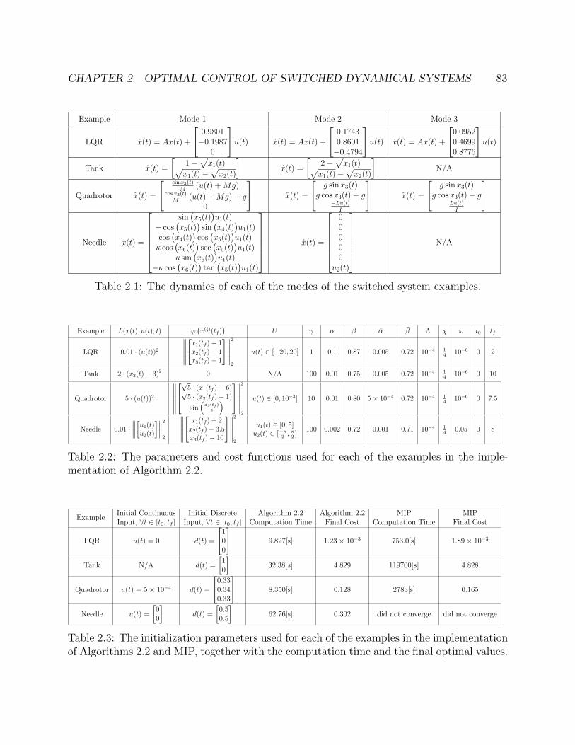
CHAPTER 2. OPTIMAL CONTROL OF SWITCHED DYNAMICAL SYSTEMS 83
Example Mode 1 Mode 2 Mode 3
LQR x(t) = Ax(t) +
0.9801−0.1987
0
u(t) x(t) = Ax(t) +
0.17430.8601−0.4794
u(t) x(t) = Ax(t) +
0.09520.46990.8776
u(t)
Tank x(t) =
[1−
√x1(t)√
x1(t)−√x2(t)
]x(t) =
[2−
√x1(t)√
x1(t)−√x2(t)
]N/A
Quadrotor x(t) =
sinx3(t)M
(u(t) +Mg)cosx3(t)
M(u(t) +Mg)− g
0
x(t) =
g sinx3(t)g cosx3(t)− g
−Lu(t)I
x(t) =
g sinx3(t)g cosx3(t)− g
Lu(t)I
Needle x(t) =
sin(x5(t)
)u1(t)
− cos(x5(t)
)sin(x4(t)
)u1(t)
cos(x4(t)
)cos(x5(t)
)u1(t)
κ cos(x6(t)
)sec(x5(t)
)u1(t)
κ sin(x6(t)
)u1(t)
−κ cos(x6(t)
)tan(x5(t)
)u1(t)
x(t) =
00000
u2(t)
N/A
Table 2.1: The dynamics of each of the modes of the switched system examples.
Example L(x(t), u(t), t) ϕ(x(ξ)(tf )
)U γ α β α β Λ χ ω t0 tf
LQR 0.01 · (u(t))2
∥∥∥∥∥∥x1(tf )− 1x2(tf )− 1x3(tf )− 1
∥∥∥∥∥∥2
2
u(t) ∈ [−20, 20] 1 0.1 0.87 0.005 0.72 10−4 14
10−6 0 2
Tank 2 · (x2(t)− 3)2 0 N/A 100 0.01 0.75 0.005 0.72 10−4 14
10−6 0 10
Quadrotor 5 · (u(t))2
∥∥∥∥∥∥∥√
5 · (x1(tf )− 6)√5 · (x2(tf )− 1)
sin(x3(tf )
2
)∥∥∥∥∥∥∥
2
2
u(t) ∈ [0, 10−3] 10 0.01 0.80 5× 10⁻⁴ 0.72 10−4 14
10−6 0 7.5
Needle 0.01 ·∥∥∥∥[u1(t)u2(t)
]∥∥∥∥2
2
∥∥∥∥∥∥ x1(tf ) + 2x2(tf )− 3.5x3(tf )− 10
∥∥∥∥∥∥2
2
u1(t) ∈ [0, 5]u2(t) ∈ [−π
2, π
2]
100 0.002 0.72 0.001 0.71 10−4 14
0.05 0 8
Table 2.2: The parameters and cost functions used for each of the examples in the imple-mentation of Algorithm 2.2.
ExampleInitial Continuous Initial Discrete Algorithm 2.2 Algorithm 2.2 MIP MIPInput, ∀t ∈ [t0, tf ] Input, ∀t ∈ [t0, tf ] Computation Time Final Cost Computation Time Final Cost
LQR u(t) = 0 d(t) =
100
9.827[s] 1.23× 10⁻³ 753.0[s] 1.89× 10⁻³
Tank N/A d(t) =
[10
]32.38[s] 4.829 119700[s] 4.828
Quadrotor u(t) = 5× 10⁻⁴ d(t) =
0.330.340.33
8.350[s] 0.128 2783[s] 0.165
Needle u(t) =
[00
]d(t) =
[0.50.5
]62.76[s] 0.302 did not converge did not converge
Table 2.3: The initialization parameters used for each of the examples in the implementationof Algorithms 2.2 and MIP, together with the computation time and the final optimal values.
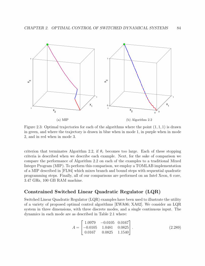
CHAPTER 2. OPTIMAL CONTROL OF SWITCHED DYNAMICAL SYSTEMS 84
1
1
1
x1
x2
x3
(a) MIP
0
1
0
1
0
1
x1
x2
x3
(b) Algorithm 2.2
Figure 2.3: Optimal trajectories for each of the algorithms where the point (1, 1, 1) is drawnin green, and where the trajectory is drawn in blue when in mode 1, in purple when in mode2, and in red when in mode 3.
criterion that terminates Algorithm 2.2, if θτ becomes too large. Each of these stoppingcriteria is described when we describe each example. Next, for the sake of comparison wecompare the performance of Algorithm 2.2 on each of the examples to a traditional MixedInteger Program (MIP). To perform this comparison, we employ a TOMLAB implementationof a MIP described in [FL94] which mixes branch and bound steps with sequential quadraticprogramming steps. Finally, all of our comparisons are performed on an Intel Xeon, 6 core,3.47 GHz, 100 GB RAM machine.
Constrained Switched Linear Quadratic Regulator (LQR)
Switched Linear Quadratic Regulator (LQR) examples have been used to illustrate the utilityof a variety of proposed optimal control algorithms [EWA06; XA02]. We consider an LQRsystem in three dimensions, with three discrete modes, and a single continuous input. Thedynamics in each mode are as described in Table 2.1 where:
A =
1.0979 −0.0105 0.0167−0.0105 1.0481 0.08250.0167 0.0825 1.1540
. (2.289)
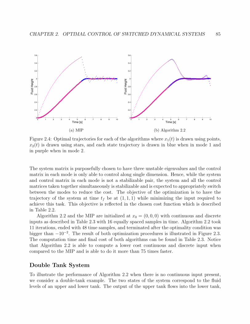
CHAPTER 2. OPTIMAL CONTROL OF SWITCHED DYNAMICAL SYSTEMS 85
0 1 2 3 4 5 6 7 8 9 102
2.2
2.4
2.6
2.8
3
3.2
3.4
3.6
Flu
id H
eig
ht
Time [s]
(a) MIP
0 1 2 3 4 5 6 7 8 9 102
2.2
2.4
2.6
2.8
3
3.2
3.4
3.6
Flu
id H
eig
ht
Time [s]
(b) Algorithm 2.2
Figure 2.4: Optimal trajectories for each of the algorithms where x1(t) is drawn using points,x2(t) is drawn using stars, and each state trajectory is drawn in blue when in mode 1 andin purple when in mode 2.
The system matrix is purposefully chosen to have three unstable eigenvalues and the controlmatrix in each mode is only able to control along single dimension. Hence, while the systemand control matrix in each mode is not a stabilizable pair, the system and all the controlmatrices taken together simultaneously is stabilizable and is expected to appropriately switchbetween the modes to reduce the cost. The objective of the optimization is to have thetrajectory of the system at time tf be at (1, 1, 1) while minimizing the input required toachieve this task. This objective is reflected in the chosen cost function which is describedin Table 2.2.
Algorithm 2.2 and the MIP are initialized at x0 = (0, 0, 0) with continuous and discreteinputs as described in Table 2.3 with 16 equally spaced samples in time. Algorithm 2.2 took11 iterations, ended with 48 time samples, and terminated after the optimality condition wasbigger than −10−2. The result of both optimization procedures is illustrated in Figure 2.3.The computation time and final cost of both algorithms can be found in Table 2.3. Noticethat Algorithm 2.2 is able to compute a lower cost continuous and discrete input whencompared to the MIP and is able to do it more than 75 times faster.
Double Tank System
To illustrate the performance of Algorithm 2.2 when there is no continuous input present,we consider a double-tank example. The two states of the system correspond to the fluidlevels of an upper and lower tank. The output of the upper tank flows into the lower tank,

CHAPTER 2. OPTIMAL CONTROL OF SWITCHED DYNAMICAL SYSTEMS 86
−1 7−1
3
x1
x2
(a) MIP
−1 7−1
3
x1
x2
(b) Algorithm 2.2
Figure 2.5: Optimal trajectories for each of the algorithms where the point (6, 1) is drawnin green, the trajectory is drawn in blue when in mode 1, in purple when in mode 2, and inred when in mode 3. Also, the quadrotor is drawn in black and the normal direction to theframe is drawn in gray.
the output of the lower tank exits the system, and the flow into the upper tank is restrictedto either 1 or 2. The dynamics in each mode are then derived using Toricelli’s Law and aredescribe in Table 2.1. The objective of the optimization is to have the fluid level in the lowertank track 3 and this is reflected in the chosen cost function described in Table 2.2.
Algorithm 2.2 and the MIP are initialized at x0 = (0, 0) with a discrete input described inTable 2.3 with 128 equally spaced samples in time. Algorithm 2.2 took 67 iterations, endedwith 256 time samples, and terminated after the optimality condition was bigger than −10−2.The result of both optimization procedures is illustrated in Figure 2.4. The computationtime and final cost of both algorithms can be found in Table 2.3. Notice that Algorithm 2.2is able to compute a comparable cost discrete input compared to the MIP and is able to doit nearly 3700 times faster.
Quadrotor Helicopter Control
Next, we consider the optimal control of a quadrotor helicopter in 2D using a model describedin [Gil+11]. The evolution of the quadrotor can be defined with respect to a fixed 2D referenceframe using six dimensions where the first three dimensions represent the position along ahorizontal axis, the position along the vertical axis and the roll angle of the helicopter,respectively, and the last three dimensions represent the time derivative of the first threedimensions. We model the dynamics as a three mode switched system (the first modedescribes the dynamics of going up, the second mode describes the dynamics of moving tothe left, and the third mode describes the dynamics of moving to the right) with a singleinput as described in Table 2.1 where L = 0.3050 meters, M = 1.3000 kilograms, I = 0.0605kilogram meters squared, and g = 9.8000 meters per second squared. The objective of theoptimization is to have the trajectory of the system at time tf be at position (6, 1) with a

CHAPTER 2. OPTIMAL CONTROL OF SWITCHED DYNAMICAL SYSTEMS 87
−4
3
0
12
x2
x1
x3
(a) Algorithm 2.2 Final Result
0 1 2 3 4 5 6 7 80
0.2
0.4
0.6
0.8
1
Time [s]d
1
0 1 2 3 4 5 6 7 80
0.2
0.4
0.6
0.8
1
Time [s]
d2
(b) Algorithm 2.2 Final Discrete Input
Figure 2.6: Optimal trajectory and optimal discrete inputs generated by Algorithm 2.2,where the point (−2, 3.5, 10) is drawn in green and obstacles are drawn in gray.
zero roll angle while minimizing the input required to achieve this task. This objective isreflected in the chosen cost function which is described in Table 2.2. A state constraint isadded to the optimization to ensure that the quadrotor remains above ground.
Algorithm 2.2 and the MIP are initialized at position (0, 1) with a zero roll angle, withzero velocity, with continuous and discrete inputs as described in Table 2.3, and with 64equally spaced samples in time. Algorithm 2.2 took 31 iterations, ended with 192 timesamples, and terminated after the optimality condition was bigger than −10−4. The resultof both optimization procedures is illustrated in Figure 2.5. The computation time and finalcost of both algorithms can be found in Table 2.3. Notice that Algorithm 2.2 is able tocompute a lower cost continuous and discrete input when compared to the MIP and is ableto do it more than 333 times faster.
Bevel-Tip Flexible Needle
Bevel-tip flexible needles are asymmetric needles that move along curved trajectories whena forward pushing force is applied. The 3D dynamics of such needles has been describedin [KC07] and the path planning in the presence of obstacles has been heuristically consideredin [Dui+08]. The evolution of the needle can be defined using six dimensions where the first

CHAPTER 2. OPTIMAL CONTROL OF SWITCHED DYNAMICAL SYSTEMS 88
three dimensions represent the position of the needle relative to the point of entry and thelast three dimensions represent the yaw, pitch and roll of the needle relative to the plane,respectively. As suggested by [Dui+08], the dynamics of the needle are naturally modeled asa two mode (the first mode describes the dynamics of going forward while the second modedescribes the dynamics of the needle turning) switched system as described in Table 2.1 withtwo continuous inputs: u1 representing the insertion speed and u2 representing the rotationspeed of the needle and where κ is the curvature of the needle and is equal to .22 inversecentimeters. The objective of the optimization is to have the trajectory of the system attime tf be at position (−2, 3.5, 10) while minimizing the input required to achieve this task.This objective is reflected in the chosen cost function which is described in Table 2.2. Astate constraint is added to the optimization to ensure that the needle remains outside ofthree spherical obstacles centered at (0 , 0 , 5), (1 , 3 , 7), and (−2 , 0 , 10) all with radius 2.
Algorithm 2.2 and the MIP are initialized at position (0, 0, 0) with continuous and discreteinput described in Table 2.3 with 64 equally spaced samples in time. Algorithm 2.2 took103 iterations, ended with 64 time samples, and terminated after the optimality conditionwas bigger than −10−3. The computation time and final cost of both algorithms can befound in Table 2.3. The MIP was unable to find any solution. The result of Algorithm 2.2is illustrated in Figure 2.6.
89
Chapter 3
Metrization and NumericalIntegration of Hybrid DynamicalSystems
Hybrid dynamical systems provide natural models for systems whose dynamics involve bothcontinuous and discrete transitions. Critical to the study of such systems is numerical simu-lation. Two approaches to numerical simulation have been considered in the hybrid systemsliterature. The first method, event detection, aims to approximate the instant in time whena trajectory crosses a switching surface by constructing a polynomial approximation to thetrajectory and then employing a root-finding scheme [Car78; EKP01; SGB91]. Unfortunatelyno proof exists that the approximation generated using this method converges to the actualtrajectory. The second method, time stepping, uses a variable-step integrator to place eventsat sample times of the discrete approximation [Bro+02]. Convergence results exist for thismethod but only for the particular case of mechanical systems with impact [PS03b; PS03a].
Here we present a numerical integration algorithm to simulate hybrid dynamical systemswhose continuous states evolve on smooth manifolds. First, we relax switching surfaces byattaching an ε-sized strip in a manner similar to the technique involved in regularizing Zenoexecutions [JEL99]. We then extend the vector field and distance metric from each domainonto these strips to obtain a relaxed hybrid dynamical system. In a manner similar to theconstruction of the hybrifold [Sim+05] and hybrid colimit [AS05], we identify subsets of therelaxed domains to construct a single metric space and develop our numerical integrationscheme on this space. Importantly, we prove that the discrete approximation generated byour algorithm converges to the original trajectory in this space. We formulate our resultin the context of autonomous vector fields to simplify the exposition, but under reasonableassumptions the same result can be applied on controlled vector fields.
Our contributions are twofold: first, in Section 3.2 we construct a metric space whichcontains the domains of a hybrid system and supports convergence analysis; second, inSection 3.3 we develop a discrete approximation technique and prove that this approximationconverges to the original trajectory. Section 3.1 describes the notation used throughout the

CHAPTER 3. METRIZATION AND INTEGRATION OF HYBRID SYSTEMS 90
chapter and Section 3.4 contains an example illustrating the numerical integration scheme.The contents of this chapter are based on the results presented in [Bur+11].
3.1 Preliminaries
Smooth Manifolds
We begin by introducing the standard mathematical objects used throughout this chapter.An extended introduction to the ideas presented herein related to manifolds can be foundin [Lee03].
Definition 3.1. A topological n–dimensional manifold is a space with the following proper-ties:
(1) M is a Hausdorff space.
(2) M is second countable.
(3) M is locally equivalent to a subset of Rn, i.e. for each p ∈M there exists a neighborhoodUp of p and a function ϕp : M → Rn such that ϕp|Up is a homeomorphism.
The last condition implies the existence of a collection of pairs of neighborhoods and func-tions. We call this collection the charts of M and denote it by {(Uα, ϕα)}α∈A for some indexset A.
Definition 3.2. A smooth n–dimensional manifold, or simply a manifold, is a topologicalmanifold, as described in Definition 3.1, such that for each α, β ∈ A the map ϕα ◦ ϕ−1
β :ϕβ(Uα ∩ Uβ)→ ϕα(Uα ∩ Uβ) is a diffeomorphism.
Definition 3.3. A manifold with boundary is a topological manifold where the range of thecharts {ϕα}α∈A is not Rn, as described in Definition 3.1, but
Hn = {(x1, . . . , xn) ∈ Rn | xn ≥ 0}. (3.1)
We define the boundary of M , denoted by ∂M , as the union of the preimages of all chartsof the set {(x1, . . . , xn) ∈ Rn | xn = 0}.
Note that the definition of manifold with boundary is a generalization of the originaldefinition of manifold, in the sense that every manifold can be seen as a manifold withboundary, where the boundary is the null set.
Definition 3.4. An embedded k–dimensional submanifold of a manifold M is a subsetS ⊂M where for each p ∈ S there exists a neighborhood Up of p and a function ϕp : M → Rn
such that ϕp(Up ∩ S) ⊂ {(x1, . . . , xn) ∈ Rn | xk+1 = · · · = xn = 0}. We also say that S hascodimension equal to (n− k).

CHAPTER 3. METRIZATION AND INTEGRATION OF HYBRID SYSTEMS 91
Given a manifold with boundary M , ∂M is clearly an embedded (n − 1)–dimensionalsubmanifold, as described in Definition 3.3.
Definition 3.5. Given a smooth manifold M , we say that C∞(M) is the set of all theinfinitely smooth functions from M to R.
Definition 3.6. Given a manifold M , the tangent space at p ∈M , denoted by TpM , is theset of all maps V : C∞(M)→ R such that, for any f, g ∈ C∞(M),
V (fg) = f(p)V (g) + g(p)V (f). (3.2)
If the manifold is Rn, then, given p ∈ Rn, TpRn is exactly the set of all directionalderivatives of smooth functions evaluated at p, i.e. for each V ∈ TpM there exists a directiond ∈ Rn such that
V (f) = limλ→0
f(p+ λd)− f(p)
λ. (3.3)
As shown in Section 3 in [Lee03], Definition 3.6 is the right definition for the tangent spacein the sense that we can intuitively match every element in TpM with a vector belonging toa tangential plane to p ∈ M . Also, given a smooth curve γ : R → M , a natural definitionfor its derivative at each t ∈ R, denoted by γ(t), is exactly a vector in Tγ(t)M .
The most important result obtained from Definition 3.6 is that for each p ∈ M , TpM isan n–dimensional vector space, thus isomorphic to Rn (Lemmas 3.9 and 3.10 in [Lee03]).
Definition 3.7. The tangent bundle of a manifold M , denoted by TM , is the disjoint unionof all the tangent spaces, i.e. TM =
∐p∈M TpM . In other words, the elements in TM are
pairs of the form (p, V ) where p ∈M and V ∈ TpM .
Definition 3.8. A vector field in a manifold M is a map F : M → TM such that, for eachp ∈M , F (p) ∈ TpM .
Definition 3.9. Given two manifolds M and N and a smooth function F : M → N , thepushforward at p ∈ M , denoted by F∗|p : TpM → TF (p)N , is defined as
(F∗|p(V )
)(f) =
V (f ◦ F ).
In practice, the pushforward can be understood as the Jacobian matrix of F evaluatedat p, taking vectors from TpM to TF (p)N .
Definition 3.10. Given a smooth vector field F : M → TM and a point p ∈M , the integralcurve of F with initial condition p, denoted x : I →M , where I ⊂ R is an interval containingthe origin, is a curve satisfying:
x(t) = F(x(t)
), x(0) = p, ∀t ∈ I. (3.4)
Moreover, we say that x is a maximal integral curve of V if for any other integral curvex : I →M of F with initial condition p, I ⊂ I.

CHAPTER 3. METRIZATION AND INTEGRATION OF HYBRID SYSTEMS 92
Theorem 17.8 in [Lee03] proves all the fundamental results for integral curves, namelythat for every smooth vector field there exists a unique maximal smooth integral curve. Also,Theorem 17.11 in [Lee03] proves that every smooth vector field in a compact manifold has amaximal integral curve whose domain is R, which is a particular case of the well known resultfor ordinary differential equations about the existence and uniqueness of solutions when thevector field is Lipschitz continuous (see Section 2.4.1 in [Vid02] for a standard version of thisresult).
Definition 3.11. A Riemannian metric at p ∈ M is a smooth bilinear map gp : TpM ×TpM → R, such that gp(V,W ) = gp(W,V ) for each V,W ∈ TpM , and gp(V, V ) > 0 wheneverV 6= 0.
A Riemannian metric on M is a collection of Riemannian metrics at each point in Mforming a smooth map g : TM × TM → R.
A Riemannian manifold is a pair (M, g) where M is a manifold (possibly with boundary)and g is a Riemannian metric on M .
We can define an induced distance by the Riemannian metric on a Riemannian manifold,denoted d : M ×M → [0,∞), to be the infimum of the length of piece–wise smooth curvesbetween the arguments of d, i.e. if we define the length of a curve γ : [0, T ]→M by:
L(γ) =
∫ T
0
√gγ(t)
(γ(t), γ(t)
)dt, (3.5)
then the metric d is defined by:
d(p, q) = inf {L(γ) | γ : [0, T ]→M piece–wise smooth, γ(0) = p, and γ(T ) = q}. (3.6)
A fundamental result in Riemannian manifolds is that its induced metric d generates thetopology of M (see Lemma 6.2 in [Lee97] for manifolds without boundary, and Lemma 2in [AA81] for manifold with boundary). Also note that given V ∈ TpM , the map ‖V ‖g =√gp(V, V ) is indeed a norm in TpM .
Definition 3.12. Given Wp ⊂ TpM , a neighborhood of 0 ∈ TpM , we say that a retractionat p ∈M is a map βp : Wp →M that is differentiable at the origin satisfying:
(1) βp(0) = p.
(2) (βp)∗|0 ≡ idTpM , where we use the canonical identification of every element in T0 (TpM)to its analogous in TpM , and idTpM : TpM → TpM is the identity function.
A retraction on M is a collection of retractions at each point in M forming a mapβ : W →M , where W ⊂ TM is the disjoint union of neighborhoods Wp.

CHAPTER 3. METRIZATION AND INTEGRATION OF HYBRID SYSTEMS 93
The intuition behind retractions is closely related to the concept of first-order approx-imations to curves. Indeed, given a smooth curve γ : R → M , t ∈ R, its tangent vectorV = γ(t) ∈ TpM at t, and a retraction βγ(t), a first-order approximation of γ(t+λ), for smallvalues of λ, is βγ(t)(λV ). Moreover, if M = Rn then the canonical retraction is βp(V ) = p+V .
Retractions are defined to preserve first derivatives around the origin, as stated in Condi-tion 2 in Definition 3.12. Even though we do not make use of it in our result, the most impor-tant retraction in a Riemannian manifold is the Exponential Map (see Section 5 in [Lee97])which preserves the derivatives of any order.
Hybrid Dynamical Systems
Motivated by the definitions of hybrid systems presented in [BBM98; JEL99; Lyg+99;Sim+05], we begin by defining the class of hybrid systems of interest.
Definition 3.13. A hybrid dynamical system is a tuple H = (J ,Γ,D,B,F ,G,R), where:
• J is a finite set indexing the discrete states of H.
• Γ ⊂ J × J is the set of edges, forming a directed graph structure over J .
• D = {Dj}j∈J is the set of domains, where each Dj is a compact connected smoothnj-dimensional Riemannian manifold with boundary, with Riemannian metric gj andinduced distance dj.
• B = {βj}j∈J is the set of retractions, where βj is a retraction defined on Dj.
• F = {Fj}j∈J is the set of vector fields, where each Fj is a vector field defined on Dj.
• G = {Ge}e∈Γ is the set of guards, where G(j,j′) ⊂ ∂Dj is a guard in mode j ∈ J whichdefines a transition to mode j′ ∈ J .
• R = {Re}e∈Γ is the set of reset maps, where R(j,j′) : G(j,j′) → ∂Dj′ is a continuousmap.
A diagram presenting a three mode hybrid system is shown in Figure 3.1.We make the following assumptions on the vector fields, guards, reset maps, and retrac-
tions:
Assumption 3.14. Given j ∈ J , Fj is Lipschitz continuous. That is, for each chart
(Uα, ϕα) of Dj, the function Fj : Uα → TRnj , defined by Fj(p) =((ϕα)∗ ◦ Fj ◦ ϕ−1
α
)(p), is
Lipschitz continuous.
Assumption 3.15. The guards do not intersect. That is, for each pair of edges e1, e2 ∈ Γ,with e1 6= e2, Ge1 ∩Ge2 = ∅.

CHAPTER 3. METRIZATION AND INTEGRATION OF HYBRID SYSTEMS 94
R(2,1)
F1
D1
F2
D3
D2
F3
G(2,3)
G(1,2) G(2,1)
G(3,1)
R(3,1)R(2,3)
R(1,2)
Figure 3.1: Diagram of a hybrid dynamical system with three modes.
Assumption 3.16. The guards are closed embedded submanifolds with codimension 1. Also,the image of each reset map is a closed set.
Note that, since reset maps are continuous, Assumption 3.16 implies that the guards arealso closed sets.
Assumption 3.17. The pushforward of each retraction in each chart is Lipschitz with respectto its point of evaluation, i.e. given a chart ϕα on Dj and a neighborhood of the origin
Wp ⊂ TpRnj , the function βp(V ) : Wp → Rnj , defined by βp(V ) =(ϕα ◦ (βj)p ◦ (ϕα)−1
∗)(V ),
has a pushforward, denoted by (βp)∗|V that is Lipschitz with respect to its point of evaluationV .
Assumptions 3.14 and 3.15 are sufficient to ensure the existence and uniqueness of exe-cutions of hybrid dynamical systems as we prove in Lemma 3.32. Assumption 3.16 allows usto metrize our relaxed domain in Section 3.2. Assumption 3.17 is critical in ensuring thatthe numerical integration scheme described in Section 3.3 is properly defined.
3.2 Relaxation and Metrization of Hybrid Dynamical
Systems
Rather than approximating the time instant when a trajectory intersects a guard, we proveconvergence of the numerical integration scheme described in the next section by relaxingthe hybrid dynamical system. First, we relax hybrid domains along their guards and extendthe definition of the domain’s metric, vector field, and retraction onto this relaxation. Next,we attach the disparate domains to each other via a topological quotient and construct asingle metric space in which we can prove convergence.
The main mathematical tool behind the final result in this section is that we can cre-ate an equivalence relation that relates each relaxed guard, Gε
e, with its image through its

CHAPTER 3. METRIZATION AND INTEGRATION OF HYBRID SYSTEMS 95
corresponding reset map, Rεe
(Gεe
). Formally, given a topological space S and a function
f : A→ B, A,B ⊂ S, we define the following equivalence relation:
Λf ={
(a, b) ∈ S × S | a ∈ f−1(b), or b ∈ f−1(a), or a = b}, (3.7)
and we say that a, b ∈ S are related, denoted by af∼ b, if (a, b) ∈ Λf . It is clear that Λf
defines an equivalence relation, since it is reflexive, symmetric, and transitive. We denotethe quotient of S under Λf by S
Λf. Also, in this case we say that the equivalence class of
x ∈ S is [x]f ={a ∈ S | a f∼ x
}.
Another useful tool from graph theory is the concept of neighborhood in a graph. Usingthe same notation as in Definition 3.13, given a node j ∈ J , we say that the neighborhoodof j is
Nj = {e ∈ J × J | ∃j′ ∈ J s.t. e = (j, j′) ∈ Γ}. (3.8)
We begin by defining the relaxation of Dj, a single domain of a hybrid system. Therelaxation is accomplished by first “stretching” the guards belonging to Dj by attaching anε-sized strip along each guard. As we show in the next section, this eliminates the need toexactly detect guard satisfaction, which is fundamental in order to create an implementablecomputational scheme.
Definition 3.18. Let H be a hybrid dynamical systems as in Definition 3.13. Given e ∈Γ, we say that Sεe = Ge × [0, ε] is the strip associated to guard Ge. Given j ∈ J , letιj :
∐e∈Nj Ge →
∐e∈Nj S
εe be the canonical identification ιj(p) = (p, 0) in its corresponding
strip.Then, the relaxation of Dj is defined by:
Dεj =
Dj
∐(∐e∈Nj S
εe
)Λιj
, (3.9)
where Λιj is defined as in Equation (3.7).
Note that, since Ge, for e ∈ Nj, is a closed embedded submanifold of ∂Dj by Assump-tion 3.16, Sεe is a compact smooth manifold.
A point on a strip Sεe of Dj is defined using nj coordinates (z1, . . . , znj−1, τ), shortened(ζ, τ), where the final coordinate, τ , is called the transverse coordinate and is the distancealong the interval [0, ε]. An illustration of the quotient process taking place in Definition 3.18together with the definition of coordinates in each strip is shown in Figure 3.2. In thedefinitions and results below we slightly abuse the notation in the following way: givenj ∈ J , e ∈ Nj, and p ∈ Ge, we say that (p, 0) ∈ Sεe , where what we mean is that ιj(p) ∈ Sεe ,with ιj as in Definition 3.18.
We can construct coordinate charts for relaxations by extending the existing coordinatecharts in our original space.

CHAPTER 3. METRIZATION AND INTEGRATION OF HYBRID SYSTEMS 96
D1 ε
G(1,2) Sε(1,2)
G(1,3)
Sε(1,3)
τ
ζ
τ
ζ
Λιj−−−−−→
D1
G(1,2)
G(1,3)
Sε(1,3)
Sε(1,2)
ε
Figure 3.2: Left: disjoint union of Dj and all its strips {Sεe}e∈Nj . Right: relaxed domain Dεj
after taking the quotient with the relation Λιj .
Definition 3.19. Let α ∈ A and (Uα, ϕα) be a chart on Dj. If Uα is not a boundary chart,then its relaxation (U ε
α, ϕεα) equals the original chart. Otherwise, let ια : ∂Uα → ∂Uα × {0}
be the canonical identification ια(p) = (p, 0).Then the relaxation of Uα is:
U εα =
Uα∐(
∂Uα × [0, ε])
Λια
, (3.10)
where Λια is as defined in Equation (3.7), and the relaxation of ϕα is:
ϕεα(x) =
{ϕα(x) if x ∈ Uα,(ϕα(ζ), τ
)if x = (ζ, τ) ∈ (∂Uα × [0, ε]).
(3.11)
Note that ϕεα|Uεα is a homeomorphism, and that the relaxation of Uα is done in the samespirit as the relaxation of Dj in Definition 3.18.
Next, we develop a metric on each relaxed domain. We aim to endow each relaxed domainDεj with a metric dεj : Dε
j × Dεj → [0,∞) which restricts to dj on Dj. To achieve this, we
first define a metric on each strip and then prove that the metric induced by the quotientstructure of the relaxation is actually a metric on Dε
j with the desired property.
Definition 3.20. Let j ∈ J and e ∈ Nj, where Nj is as in Equation (3.8). Then, the metricdSεe : Sεe × Sεe → [0,∞) on the strip Sεe is:
dSεe((ζ, τ), (ζ ′, τ ′)
)= dj(ζ, ζ
′) + |τ − τ ′| . (3.12)
Before we continue we will define the simplest possible metric for the disjoint union ofsets in metric spaces.

CHAPTER 3. METRIZATION AND INTEGRATION OF HYBRID SYSTEMS 97
Definition 3.21. Let S1 and S2 be sets in metric spaces, with metric d1 and d2 respectively.Then we say that d : S1
∐S2 × S1
∐S2 → [0,∞] is the disjoint metric of S1
∐S2, defined
by:
d(x, y) =
d1(x, y) if x, y ∈ S1,
d2(x, y) if x, y ∈ S2,
∞ otherwise.
(3.13)
Using Definition 3.21 we can define dεj to be the disjoint metric of Dj
∐(∐e∈Nj S
εe
).
Then the function dεj : Dεj ×Dε
j → [0,∞) defined by:
dεj(x, y) = inf
{k∑i=1
dεj(pi, qi) | k ∈ N, x = p1, y = qk, qiιj∼ pi+1 ∀i ∈ {1, . . . , k − 1}
},
(3.14)where ιj is as in Definition 3.18, is a semi-metric on Dε
j , i.e. it is non-negative, symmetric, andsatisfies the Triangle Inequality (Definition 3.1.12 in [BBI01]), but in general, dεj(x, y) = 0
may not imply xιj∼ y. The following theorem establishes that, in fact, dεj is a metric on Dε
j .
Theorem 3.22. For each j ∈ J , the function dεj, as in Equation (3.14), is a metric on Dεj ,
as in Definition 3.18.
Proof. We already know that dεj is a semi-metric, so all we must show is that [x]ιj = [y]ιjwhenever dεj
([x]ιj , [y]ιj
)= 0, where ιj is as in Definition 3.18.
Let e ∈ Nj. Each x ∈ Dj \ Ge has a dj-ball that is disjoint from Ge, since Ge is closedby Assumption 3.16, therefore [x]ιj = {x} is a singleton. Similarly each x ∈ Sεe \ (Ge × {0})has a dSεe -ball which is disjoint from Ge × {0}, therefore [x]ιj = {x} is a singleton. Finally,
each x ∈ Ge has a dj-ball and a dSεe -ball (defined in their appropriate space) disjoint fromany other y ∈ Ge, therefore [x]ιj = {x, (x, 0)}.
This argument is true for each e ∈ Nj, and thus establishes that dεj is a metric on Dεj .
The following Lemma, whose proof we omit, gives us a basic estimate of the relaxedmetric dεj .
Lemma 3.23. Let dεj be defined as in Equation (3.14), and let e ∈ Nj, where Nj is as inEquation (3.7).
Then, given x, y ∈ Dj, dεj(x, y) ≤ dj(x, y). Similarly, given x, y ∈ Sεe , dεj(x, y) ≤ dSεe (x, y).
Next, we extend the vector field onto the strip:
Definition 3.24. Given j ∈ J , for each e ∈ Nj, where Nj is as in Equation (3.7), letthe vector field on the strip Sεe , denoted FSεe , be the unit vector pointing outward along thetransverse direction, i.e. FSεe (ζ, τ) = ∂
∂τ.

CHAPTER 3. METRIZATION AND INTEGRATION OF HYBRID SYSTEMS 98
D1 ε
Sε(1,2)
Sε(1,3)
Figure 3.3: Relaxed vector field F εj on Dε
j .
Then, the relaxation of Fj is:
F εj (x) =
{Fj(x) if x ∈ Dj,
FSεe (x) if x ∈ Ge × (0, ε], ∀e ∈ Nj.(3.15)
Note that the relaxation of the vector field is generally not continuous along each Ge,for e ∈ Nj. As we will show in Lemma 3.33, this discontinuous vector field does not lead toexecutions described as Filippov solutions of a switched differential equation [Fil88], sincethe vector field on the strips always points away of the guard. An illustration of the relaxedvector field F ε
j on Dεj is shown in Figure 3.3.
In contrast to the vector field, which we explicitly extend throughout the strip, we donot require an explicit form for our relaxed retractions. Instead, we require that any relaxedretraction centered at points sufficiently close to a guard has a range that includes the strip.
Definition 3.25. Let j ∈ J , and e ∈ Nj, where Nj is as in Equation (3.7). Also, letp ∈ Dj \ ∂Dj, and βp : Wp → Dj a retraction on p, as in Definition 3.12.
If β−1p
(G(j,j′)
)∩Wp = ∅, then any relaxation of βp equals βp. Otherwise, we say that a
relaxation of βp is any differentiable function βεp : Up → Dεj , with Up an open set containing
Wp, so that βεp agrees with βp on Wp.The relaxation of βj, denoted by βεj , is just the collection of relaxations of βεp on the
interior of Dj.
Constructing a relaxed retraction is always possible by means of local relaxed coordinatecharts, but we omit the proof since it is outside the scope of our result. Note in particularthat if the domain Dj is a subset of Rnj , then a relaxation of a retraction βp(v) = p+v couldbe constructed by simply extending the domain of βp and setting βεp(v) = p + v for each vin the new domain.
We simultaneously relax each hybrid domain to define the relaxation of a hybrid dy-namical system and then attach the disparate domains of the relaxed system together toconstruct a metric space.
CHAPTER 3. METRIZATION AND INTEGRATION OF HYBRID SYSTEMS 99
Definition 3.26. Let H be a hybrid system as in Definition 3.13. The relaxation of H is atuple Hε = (J ,Γ,Dε,Bε,F ε,Gε,Rε), where:
• Dε ={Dεj
}j∈J is the set of relaxations of the domains D, as in Definition 3.18, with
metrics{dεj}j∈J , as in Equation (3.14).
• Bε ={βεj}j∈J is a set of relaxations of the retractions B, as in Definition 3.25.
• F ε ={F εj
}j∈J is the set of relaxations of the vector fields F , as in Definition 3.24.
• Gε = {Gεe}e∈Γ is the set of relaxations of the guards G, where, given e = (j, j′), each
guard Ge ⊂ ∂Dj is relaxed to Gεe = Ge × {ε} ⊂ ∂Dε
j .
• Rε = {Rεe}e∈Γ is the set of relaxations of the reset maps R, where, given e = (j, j′),
Rεe : Gε
e → ∂Dj′ is defined by Rεe(ζ, τ) = Re(ζ).
Now we can define a new metric space where the executions of hybrid systems can benaturally described. This definition is, in practice, completely equivalent to the hybrid colimitpresented in [AS05].
Definition 3.27. Let Hε be a relaxed hybrid system as in Definition 3.26. Also, let
Rε :∐e∈Γ
Gεe →
∐j∈J
Dεj , (3.16)
the function that represents all reset maps as a unified function, i.e. Rε(p) = Rεe(p) whenever
p ∈ Gεe.
Then, the relaxed hybrid quotient space of a relaxed hybrid dynamical system Hε is:
Mε =
∐j∈J D
εj
ΛRε, (3.17)
where ΛRε is as in Equation (3.7).
The illustration in Figure 3.4 shows the details about the construction in Definition 3.27.As we did in the definition of the relaxed metric dεj , we say that µε is the disjoint metric on∐
j∈J Dεj based on the individual metrics
{dεj}j∈J , as in Definition 3.21. Then the function
µε :Mε ×Mε → [0,∞) defined by:
µε(x, y) = inf
{k∑i=1
µε(pi, qi) | k ∈ N, x = p1, y = qk, qiRε∼ pi+1 ∀i ∈ {1, . . . , k − 1}
},
(3.18)is a semi-metric on Mε, where Rε is as in Definition 3.27. In general, µε(x, y) = 0 may not
necessarily imply xRε∼ y. The following theorem establishes the fact that µε is a metric on
Mε.

CHAPTER 3. METRIZATION AND INTEGRATION OF HYBRID SYSTEMS 100
Gε(1,2)
ε
Rε(1,2)
(Gε
(1,2)
)Dε1 Dε
2
ΛRε−−−−−−→
ε
Mε
Dε1 Dε
2
Figure 3.4: Left: disjoint union of Dε1 and Dε
2. Right: relaxed hybrid quotient space Mε
after taking the quotient with the relation ΛRε .
Theorem 3.28. The function µε is a metric on Mε.
Proof. Since, by Assumption 3.16, the image of each reset map is closed, and since we canobtain metric neighborhoods separating distinct points in Rε
e
(Gεe
)for each e ∈ Γ, the result
follows by a similar argument to the one presented in the proof of Theorem 3.22.
As we did in Lemma 3.23, the next Lemma shows that we can estimate the value of µε
using each relaxed metric dεj within a domain. We omit the proof since it follows easily fromthe definition of the metric as the infimum of all possible paths.
Lemma 3.29. Let µε be defined as in Equation (3.18), and let j ∈ J . Then given x, y ∈ Dεj ,
µε(x, y) ≤ dεj(x, y).
Perhaps the most relevant property of µε is that if y = Rεe(x) for some x ∈ Gε
e ande ∈ Γ, then µε(x, y) = 0, which is exactly what we would expect to happen if we want thetrajectories of hybrid systems to be continuous. Exploiting this property, we define a metricbetween curves on Mε.
Definition 3.30. Let I ⊂ [0,∞) a bounded interval, and µε as in Equation (3.18). Then,given any two curves x, x′ : I →Mε we define
ρεI(x, x′
)= sup
{µε(x(t), x′(t)
)| t ∈ I
}. (3.19)
Our choice of the supremum among point-wise distances in ρεI is inspired in the sup-normfor continuous real functions, since, as we show in Section 3.3, the executions of relaxed hybridsystems are continuous.
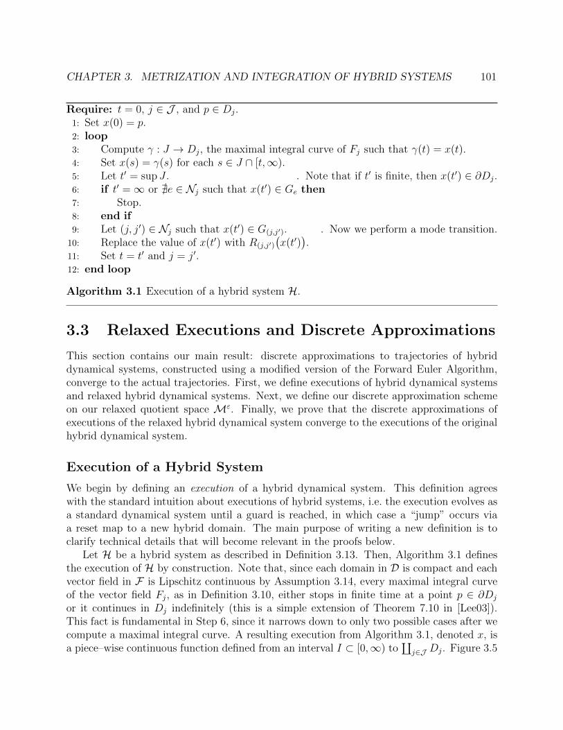
CHAPTER 3. METRIZATION AND INTEGRATION OF HYBRID SYSTEMS 101
Require: t = 0, j ∈ J , and p ∈ Dj.1: Set x(0) = p.2: loop3: Compute γ : J → Dj, the maximal integral curve of Fj such that γ(t) = x(t).4: Set x(s) = γ(s) for each s ∈ J ∩ [t,∞).5: Let t′ = sup J . . Note that if t′ is finite, then x(t′) ∈ ∂Dj.6: if t′ =∞ or @e ∈ Nj such that x(t′) ∈ Ge then7: Stop.8: end if9: Let (j, j′) ∈ Nj such that x(t′) ∈ G(j,j′). . Now we perform a mode transition.
10: Replace the value of x(t′) with R(j,j′)
(x(t′)
).
11: Set t = t′ and j = j′.12: end loop
Algorithm 3.1 Execution of a hybrid system H.
3.3 Relaxed Executions and Discrete Approximations
This section contains our main result: discrete approximations to trajectories of hybriddynamical systems, constructed using a modified version of the Forward Euler Algorithm,converge to the actual trajectories. First, we define executions of hybrid dynamical systemsand relaxed hybrid dynamical systems. Next, we define our discrete approximation schemeon our relaxed quotient space Mε. Finally, we prove that the discrete approximations ofexecutions of the relaxed hybrid dynamical system converge to the executions of the originalhybrid dynamical system.
Execution of a Hybrid System
We begin by defining an execution of a hybrid dynamical system. This definition agreeswith the standard intuition about executions of hybrid systems, i.e. the execution evolves asa standard dynamical system until a guard is reached, in which case a “jump” occurs viaa reset map to a new hybrid domain. The main purpose of writing a new definition is toclarify technical details that will become relevant in the proofs below.
Let H be a hybrid system as described in Definition 3.13. Then, Algorithm 3.1 definesthe execution of H by construction. Note that, since each domain in D is compact and eachvector field in F is Lipschitz continuous by Assumption 3.14, every maximal integral curveof the vector field Fj, as in Definition 3.10, either stops in finite time at a point p ∈ ∂Dj
or it continues in Dj indefinitely (this is a simple extension of Theorem 7.10 in [Lee03]).This fact is fundamental in Step 6, since it narrows down to only two possible cases after wecompute a maximal integral curve. A resulting execution from Algorithm 3.1, denoted x, isa piece–wise continuous function defined from an interval I ⊂ [0,∞) to
∐j∈J Dj. Figure 3.5

CHAPTER 3. METRIZATION AND INTEGRATION OF HYBRID SYSTEMS 102
x(0)
G(1,2) R(1,2)
(G(1,2)
)D1 D2
x(t′)
Figure 3.5: Mode transition of execution x in a two-mode hybrid dynamical system.
shows an example of the mode transition of an execution.Formally, given x as constructed by Algorithm 3.1 and t ∈ I, x(t) ∈
∐j∈J Dj, but we
abuse notation and say that x(t) ∈ Mε when we should say that [x]Rε ∈ Mε, where Rε isas in Definition 3.27. We make use of this fact when comparing a hybrid execution with itscorresponding relaxed execution, which we define in Algorithm 3.2.
With our definition of execution of a hybrid system in place, we can define an importantclass of executions that only exist in hybrid systems.
Definition 3.31. A Zeno execution is an execution where there exists an infinite numberof discrete transitions in a finite amount of time. Hence, there exists T ∈ R so that theexecution is only defined on I = [0, T ).
Zeno executions are important because, among other properties, they are very hardto approximate numerically since, in practice, simulating an infinite number of discretetransitions takes an infinite amount of time in any computer.
Now we show that Algorithm 3.1 produces well-defined trajectories.
Lemma 3.32. Let H be a hybrid system as in Definition 3.13, j ∈ J , and p ∈ Dj. Then,Algorithm 3.1 produces a unique maximal trajectory.
Proof. Let x : I →∐
j∈J Dj be the execution produced by Algorithm 3.1. First note thatfor each t ∈ I, x(t) is uniquely defined. Indeed, either x(t) is defined by a maximal integralcurve in Step 3, which is unique by Assumption 3.14, or it is defined as the image of a resetmap in Step 10, which is also unique by Assumption 3.15.
Now, Algorithm 3.1 can produce only three types of executions:
• x has a finite number of mode transitions and I = [0,∞).
• x has a finite number of mode transitions, I = [0, T ] for some T > 0, and x(T ) ∈ ∂Dj
for some j ∈ J .

CHAPTER 3. METRIZATION AND INTEGRATION OF HYBRID SYSTEMS 103
Require: t = 0, j ∈ J , and p ∈ Dj.1: Set xε(0) = p.2: loop3: Compute γ : J → Dj, the maximal integral curve of Fj such that γ(t) = xε(t).4: Set xε(s) = γ(s) for each s ∈ J ∩ [t,∞).5: Let t′ = sup J . . Note that if t′ is finite, then xε(t′) ∈ ∂Dj.6: if t′ =∞ or @e ∈ Nj such that x(t′) ∈ Sεe then7: Stop.8: end if9: Let (j, j′) ∈ Nj such that x(t′) = (q, 0) ∈ Sε(j,j′).
. Now we perform a mode transition.10: Set xε(t′ + τ) = (q, τ) for each τ ∈ [0, ε].
. Note that [xε(t′ + ε)]Rε =[Rε
(j,j′)
(xε(t′ + ε)
)]Rε
.
11: Set t = t′ + ε and j = j′.12: end loop
Algorithm 3.2 Relaxed execution of a relaxed hybrid system Hε.
• x is a Zeno execution and I = [0, T ) for some T > 0.
In either case we obtain a maximal trajectory, since its time domain cannot be extended.
Relaxed Execution of a Hybrid System
Now we define the relaxed execution of a hybrid dynamical system. The main idea hereis that, once the execution reaches a guard, we continue integrating over the strip with itstrivial vector field FSεe , as in Definition 3.24.
Let H be a hybrid system, as in Definition 3.13, and Hε its relaxation, as in Defini-tion 3.26. Then, Algorithm 3.2 defines a relaxed execution of Hε by construction. Theresulting relaxed execution, denoted xε, is continuous function defined from an intervalI ⊂ [0,∞) to Mε, as in Definition 3.27. Note that Algorithm 3.2 is only defined for initialconditions in Dj for some j ∈ J since the strips are artificial objects which do not appearin the original model of the system.
A very important part of Algorithm 3.2 is Step 10, since it allow us to “connect” eachmode transition, forming a continuous curve in the relaxed quotient space Mε. It is alsoimportant that our definition for the relaxed execution over the strip Sεe , also in Step 10, isexactly equal to the maximal integral curve of FSεe . In other words, we could have written ashorter version of Algorithm 3.2 by solving the maximal integral curve of the relaxed vectorfield F ε
j in Step 3, at the expense of making it harder to understand. Figure 3.6 shows anexample of the relaxed mode transition produced by this Algorithm.

CHAPTER 3. METRIZATION AND INTEGRATION OF HYBRID SYSTEMS 104
xε(0)
G(1,2) Rε(1,2)
(Gε
(1,2)
)Dε1 Dε
2
xε(t′) xε(t′ + ε)
Figure 3.6: Relaxed mode transition of the relaxed execution xε in a two-mode hybriddynamical system.
Note that, given a hybrid system H, its relaxation Hε, and an initial condition p ∈Dj, the relaxed execution of Hε produced by Algorithm 3.2 is simply a delayed versionof the execution of H produced by Algorithm 3.1, since the relaxed version has to spendadditional time on each mode transition. Also, note that our definition of relaxed executionis compatible with the execution of a regularized hybrid system as defined in [JEL99].
We omit the proof of the following Lemma since it is similar to the proof of Lemma 3.32.
Lemma 3.33. Let H be a hybrid system as in Definition 3.13, and let Hε be its relaxationas in Definition 3.26. Also, let j ∈ J and p ∈ Dj.
Then, Algorithm 3.2 produces a unique maximal trajectory.
Next, we define the types of trajectories that can be approximated.
Definition 3.34. Let H be a hybrid system, as in Definition 3.13, and Hε be its relaxation,as in Definition 3.26. Given j ∈ J and p ∈ Dj, let us denote the execution of H withinitial condition p by xp, and similarly let us denote the relaxed execution of Hε with initialcondition p by xεp.
Then, we say that xp is orbitally stable at p′ ∈Mε if, for each t ∈ I, the map p 7→ xεp(t)is continuous at p′.
Orbitally stable executions are exactly the type of execution that can be approximatedin a hybrid dynamical system [Lyg+03]. Indeed, if an execution is not orbitally stable thenthere exists a time t′ such that, if we initialize another execution arbitrarily close to xε(t′),the executions will have different sequences of discrete transitions. Classical dynamicalsystems are always orbitally stable (see Theorem 17.8 in [Lee03] for a stronger version of thisresult), hence non-orbitally stable executions are, together with Zeno executions, two of theconsequences of allowing discrete transitions as time evolves. Figure 3.7 shows the case of anon-orbitally stable execution due to a discrete transition in the boundary of a guard.

CHAPTER 3. METRIZATION AND INTEGRATION OF HYBRID SYSTEMS 105
ε
Dε1 Dε
2Mε
G(1,2)
p′
Figure 3.7: Non-orbitally stable execution at p′ of a two-mode hybrid dynamical system.
Even though we do not deal with this problem in our result, we can mention a thirdconsequence of discrete mode transitions: the evolution of a hybrid system cannot be reversedin time, as opposed to classical dynamical systems where we can always solve a differentialequation either forward or backwards in time. This problem is one of the biggest problemsin the computation of the optimal control of hybrid systems, since the costate is usuallycalculated as the solution of a differential equation backwards in time (more details can befound in [Sus99b; SC07; HT11]).
Before we state our result proving the convergence of relaxed executions as ε → 0, weintroduce a particular type of Zeno executions of interest.
Definition 3.35. Let H be a hybrid system, as in Definition 3.13, j ∈ J , and p ∈ Dj
such that x : [0, T ) → Mε, the execution of H with initial condition p as constructed byAlgorithm 3.1, is a Zeno execution as in Definition 3.31.
We say that x accumulates on p′ ∈ Mε if there exists C > 0 such that for each r > 0there exists δ > 0 satisfying:
supt∈[T−δ,T )
µε(p′, x(t)
)≤ Cε+ r. (3.20)
In practice, if a Zeno executions accumulates then it is impossible for this execution to“fill” a portion of the hybrid space while having an infinite number of discrete transitions.Examples of Zeno executions that do not accumulate can be found in [Zha+01]. Figure 3.8shows a Zeno execution that accumulates on p′. Note that p′ must belong to a guard of thehybrid system. Also, the choice of p′ is not unique in Mε for ε > 0, since we can alwayschoose the image of p′ via a reset map.
Now we state our first convergence theorem.
Theorem 3.36. Let H be a hybrid system, as in Definition 3.13, and Hε be its relaxation,as in Definition 3.26. Also, let j ∈ J , p ∈ Dj, x : I →Mε be the execution of H with initialcondition p, constructed by Algorithm 3.1, and xε be the relaxed execution of Hε with initialcondition p, constructed by Algorithm 3.2.
If x has a finite number of discrete transitions or it is a Zeno execution that accumulates,then for each J ⊂ I, where J is bounded interval,
limε→0
ρεJ(x, xε) = 0, (3.21)

CHAPTER 3. METRIZATION AND INTEGRATION OF HYBRID SYSTEMS 106
Mε
ε
Dε1 Dε
2G(1,2)
G(2,1)
p′
Figure 3.8: Zeno execution accumulating on p′ for a two mode hybrid dynamical system.
where ρεJ is as in Definition 3.30.
Proof. First, let us consider the case when x undergoes a finite number of discrete transitionson J , thus without loss of generality we can assume that J = [0, T ] for some T > 0. Let{tk}m+1
k=0 be the sequence of times at which discrete mode transitions occur, with t0 = 0 andtm+1 = T , and let {jk}mk=0 be the sequence of domains visited by the execution. Also, letε > 0 such that
(m+ 1)ε < sup {tk+1 − tk | tk+1 > tk, k ∈ {0, . . . ,m}}. (3.22)
Since the function x|[tk,tk+1) is defined on Djk , then using Lemmas 3.23 and 3.29 and thedefinition of dj in Equation (3.6), for each t, t′ ∈ [tk, tk+1), t′ ≥ t,
µε(x(t), x(t′)
)≤ djk
(x(t), x(t′)
)≤∫ t′
t
√gjk(x(s), x(s)
)ds ≤ L(t′ − t), (3.23)
where L = sup{‖Fj(p)‖gj | p ∈ Dj, j ∈ J
}, which is bounded since each Dj is compact.
Note that by definition, x|[t0,t1) = xε|[t0,t1). Let k ∈ {1, . . . ,m} such that tk+1 > tk. Thenwe compute a bound on the distance µε
(xε(t), x(t)
)for t ∈ [tk, tk+1), by considering three
cases:
(1) t ∈ [tk, tk + (k − 1)ε): In this case xε(t) ∈ Djk−1and x(t) ∈ Djk by our choice of ε in
Equation (3.22). Moreover, xε(t) = x(t− (k − 1)ε
). If we define x(t−k ) = limt→t−k
x(t),
then by Equation (3.23):
µε(xε(t), x(t)
)≤ µε
(x(t− (k − 1)ε
), x(t−k )
)+ µε
(x(t−k ), x(tk)
)+ µε
(x(tk), x(t)
)≤ L(k − 1)ε+ ε+ L(k − 1)ε.
(3.24)
(2) t ∈ [tk + (k − 1)ε, tk + kε): In this case xε(t) ∈ Sε(jk−1,jk) and x(t) ∈ Djk , hence:
µε(xε(t), x(t)
)≤ µε
(xε(t), x(tk)
)+ µε
(x(tk), x(t)
)≤ ε+ Lkε.
(3.25)
CHAPTER 3. METRIZATION AND INTEGRATION OF HYBRID SYSTEMS 107
(3) t ∈ [tk + kε, tk+1): In this case xε(t), x(t) ∈ Djk , hence xε(t) = x(t− kε) and:
µε(xε(t), x(t)
)≤ Lkε. (3.26)
If there is a sequence of ` consecutive jumps such that tk = · · · = tk+`−1 then the argument isanalogous, noting that in the case 2 the interval of interest is [tk+(k−1)ε, tk+(k+`)ε), with abound `ε+L(k+`)ε. Also, note that µε
(xε(tm+1), x(tm+1)
)≤ µε
(xε(t−m+1), x(t−m+1)
)+ε, this
last bound being an equality if there is a discrete transition exactly at t = tm+1. Therefore,putting together all the bounds above we have that for each t ∈ [0, T ]:
µε(xε(t), x(t)
)≤ (2L+ 1)mε, (3.27)
which proves the theorem if the number of transitions is finite.Next, let us consider the case when x is a Zeno execution that accumulates on p′, thus
I = [0, T ). As we did above, let {tk}∞k=0 be the sequence of times at which discrete modetransitions occur, and let {jk}∞k=0 be the sequence of domains visited by the execution. Letr > 0, and note that as a consequence of Definition 3.35 there exists C > 0 and δr > 0 suchthat µε
(p′, x(t)
)≤ Cε + r for each t ∈ [T − δr, T ). Let us denote by n(δ) the number of
discrete transitions on the interval [0, T − δ], and let ε > 0 such that:
n(δr)ε < min{tn(δr)+1 − tn(δr), δ2r
}, (3.28)
where without loss of generality we have assumed that tm(δr)+1 > tm(δr).From this choice of ε we get that both xε and x are in the same domain at t = T − δr,
hence xε(t) = x(t− n(δr)ε
), and since n(δr)ε < δ2r, then
µε(p′, xε(t)
)≤ Cε+ 2r, ∀t ∈ [T − δr, T ) . (3.29)
The conclusion follows since there exists C ′ > 0 such that, using Equations (3.27)and (3.28),
µε(xε(t), x(t)
)≤ C ′
(tn(δr)+1 − tn(δr) + ε
)+ 2r, ∀t ∈ [0, T ), (3.30)
But r > 0 was arbitrary and tn(δr)+1 − tn(δr) → 0 as r → 0 since the number of discretetransitions goes to infinity, hence ρε[0,T )(x
ε, x)→ 0 as ε→ 0 as desired.
Discrete Approximations
Now we can define the discrete approximation of a relaxed execution. As mentioned above,our discrete approximation scheme is based on the Forward Euler integration approximationfor ODE’s, modified to be applicable on Riemannian manifolds by using retractions, as inDefinition 3.12.
Given a hybrid systemH, as in Definition 3.13, and its relaxationHε, as in Definition 3.26.Then, Algorithm 3.3 defines a discrete approximation of a relaxed execution of Hε. The

CHAPTER 3. METRIZATION AND INTEGRATION OF HYBRID SYSTEMS 108
Require: h > 0, k = 0, j ∈ J , and p ∈ Dj.1: Set t0 = 0 and z(ε,h)(0) = p.2: loop3: if @t > 0 such that tFj
(z(ε,h)(tk)
)is in the domain of βεj then
4: Stop.5: end if6: Find smallest n such that h
2nFj(z(ε,h)(tk)
)is in the domain of βεj .
7: Set tk+1 = tk + h2n
.8: Set z(ε,h)(t) = βεj
(tFj(z(ε,h)(tk)
))for each t ∈ [tk, tk+1].
9: if ∃e ∈ Nj such that z(ε,h)(tk+1) ∈ Sεe then10: Let (j, j′) ∈ Nj such that z(ε,h)(tk+1) = (q, τ) ∈ Sε(j,j′).
. Now we perform a mode transition.11: Set tk+2 = tk+1 + ε− τ .12: Set z(ε,h)(t) = (q, t− tk+1 + τ) for each t ∈ [tk+1, tk+2].
. Note that[z(ε,h)(tk+2)
]Rε
=[Rε
(j,j′)
(z(ε,h)(tk+2)
)]Rε
.
13: Set k = k + 2 and j = j′.14: else15: Set k = k + 1.16: end if17: end loop
Algorithm 3.3 Discrete approximation of the execution of a relaxed hybrid system Hε.
resulting discrete approximation, for a step size h > 0, denoted by z(ε,h), is a function froma closed interval I ⊂ [0,∞) to Mε, as in Definition 3.27.
We now make a few remarks about Algorithm 3.3. First, the condition in Step 3 can onlybe satisfied, i.e. the Algorithm only stops, if z(ε,h)(tk) ∈ ∂Dk and Fj
(z(ε,h)(tk)
)is outward-
pointing, since otherwise the domain of βεj contains a Euclidean neighborhood of the origin.The intuition about outward-pointing vectors in the tangent space is very simple, these areexactly the vectors that generate curves going “out” of the manifold. More details canbe found in Section 13 in [Lee03], particularly in Lemma 13.5. Second, Step 6 effectivelyimplements a variable step size Forward Euler scheme for Riemannian manifolds, where weonly reduce the step size when we are close to the boundary of Dε
j . Third, in Step 8, note thatif Dj ⊂ Rnj then the canonical retraction (βj)p(V ) = p + V produces exactly the ForwardEuler approximation as expected. Fourth, the function z(ε,h) is continuous on Mε.
But perhaps the most important comment we can make about Algorithm 3.3 is relatedwith Step 12. Indeed, similarly to Algorithm 3.2, the curve assigned to z(ε,h) in this Step isexactly the maximal integral curve of FSεe in the strip. We explain the importance of this factwithin the context of existing algorithms. As mentioned in the introduction to this Chapter,the hardest problem to solve in the numerical integration of hybrid dynamical systems is

CHAPTER 3. METRIZATION AND INTEGRATION OF HYBRID SYSTEMS 109
G(1,2) Rε(1,2)
(Gε
(1,2)
)Dε1 Dε
2
τ
ε
z(ε,h)(tk)
z(ε,h)(0)
z(ε,h)(tk+2)
Figure 3.9: Discrete approximation z(ε,h) of a relaxed execution in a two-mode hybrid dy-namical system.
finding the guard with enough accuracy so that the reset could be applied without errors.By relaxing the guards using strips, and then endowing the strips with a trivial vector field,we can implement a scheme that does not need to find exact guard, while still evaluatingthe reset maps at exactly the points belonging to the guards. Our relaxation does introducean error in the approximation, but as we show in Theorem 3.37, the error is of order ε.
Figure 3.9 shows a discrete approximation produced by Algorithm 3.3 as it performs amode transition.
Theorem 3.37. Let H be a hybrid dynamical system, as in Definition 3.13, Hε its relaxation,as in Definition 3.26. Also, let j ∈ J , p ∈ Dj, and I = [0, T ] for some T > 0.
If the relaxed execution of Hε with initial condition p, constructed by Algorithm 3.2, has adomain that contains I and is orbitally stable, as in Definition 3.34, then there exists C > 0such that
limh→0
ρεI(xε, z(ε,h)
)= Cε, (3.31)
where ρεI is as in Definition 3.30.
Proof. We complete this proof in incremental steps, first showing the convergence of ourmodified Forward Euler scheme in Riemannian manifolds for a single domain, and thenshowing that our relaxation of the discrete transitions converge on the relaxed quotientspace Mε.
In order to simplify the first part of our argument, let us assume that the hybrid systemhas only one domain and no discrete transitions, i.e. D = {D}, F = {F}, B = {β},J = {1}, Γ = G = R = ∅. Let xε : [0, T ] → D a relaxed execution, constructed byAlgorithm 3.2, where without loss of generality we are assuming that [0, T ] belongs to thedomain of the relaxed execution. Similarly, let z(ε,h) : [0, T ] → D a discrete approximation,constructed using Algorithm 3.3. Note that we have not made any assumptions about theinitial conditions of xε or z(ε,h). Also, since we have a single domain, x and xε are identical.

CHAPTER 3. METRIZATION AND INTEGRATION OF HYBRID SYSTEMS 110
Let {tk}`k=0 ⊂ [0, T ] be the sequence of time samples derived from Algorithm 3.3, wheret0 = 0 and we remove the dependence of each tk and ` on h for notational convenience. Notethat ` does not need to be finite. Given a chart (U,ϕ), let us also define β : W → Rn,
W ⊂ TRn, and F : U → TRn, U ⊂ Rn, such that
βp(V ) =(ϕ ◦ βp ◦ ϕ−1
∗)
(V ),
F (q) =(ϕ∗ ◦ F ◦ ϕ−1
)(q),
(3.32)
and similarly denote xε = ϕ ◦ x and z(ε,h) = ϕ ◦ z(ε,h).Let us assume that given i, i′ ∈ {0, . . . , `} such that ti ≤ ti′ , both xε|[ti,ti′ ) and z(ε,h)|[ti,ti′ )
belong to the same chart. Then, using Picard’s Lemma (Lemma 5.6.3 in [Pol97]), for eacht ∈ [ti, ti′):
∥∥xε(t)− z(ε,h)(t)∥∥ ≤ eL(ti′−ti)
(∥∥xε(ti)− z(ε,h)(ti)∥∥+
i′−1∑k=i
∫ tk+1
tk
∥∥∥Fk − (βk)∗|(s−tk)FkFk
∥∥∥ ds),(3.33)
where L is the Lipschitz constant of F as defined in Assumption 3.14, Fk = F(z(ε,h)(tk)
),
and βk = βz(ε,h)(tk). Now, since the domain D is compact, β∗ is Lipschitz by Assumption 3.17,
and since β∗|0 = In as in Definition 3.12, where n is the dimension of D, then there existsC > 0 such that: ∥∥∥Fk − (βk)∗|(s−tk)Fk
Fk
∥∥∥ ≤ C(s− tk
), (3.34)
and therefore, for all t ∈ [ti, ti′),∥∥x(t)− zh(t)∥∥ ≤ eL(ti′−ti)
(∥∥xε(ti)− z(ε,h)(ti)∥∥+
1
2Ch
). (3.35)
Since D is compact, there exists a finite set of charts {(Ui, ϕi)}νi=1 such that {Ui}νi=1
form a cover of D. Without loss of generality, we can assume that Ui is closed for eachi ∈ {1, . . . , ν}, Let r0 be defined by:
r0 = infi∈{1,...,ν}
infq∈∂Ui
supj 6=i
infq′∈∂Uj∩Ui
‖ϕi(q)− ϕi(q′)‖ , (3.36)
and note that r0 > 0 since every point at a boundary of a chart is at a positive distance fromanother boundary, because the boundaries are closed and there are only a finite number ofthem. Then, for each a ∈ ϕi(Ui) there exists a neighborhood of a with radius at least r0
contained in some ϕj(Uj), j 6= i.Let (Ui, ϕi) be a chart. If q, q′ ∈ Ui then, given the curve α(t) = ϕ−1
i
((1−t)ϕi(q)+tϕi(q
′))
for t ∈ [0, 1], there exists C > 0 such that:
dj(q, q′) ≤
∫ 1
0
√g (α(t), α(t))dt ≤ C‖ϕi(q)− ϕi(q′)‖, (3.37)

CHAPTER 3. METRIZATION AND INTEGRATION OF HYBRID SYSTEMS 111
where C is in practice the supremum of ‖(ϕi)∗‖, over all i ∈ {1, . . . , ν} and all points in thecompact domain D.
Now we can finish the argument for executions on a manifold. Suppose that xε(0) andz(ε,h)(0) are in the same chart and that
∥∥xε(0)− z(ε,h)(0)∥∥ ≤ δ, then there exists s > 0 such
that xε|[0,s) and z(ε,h)|[0,s) are in the same chart. Hence, by Equation 3.35,
d(xε(s), z(ε,h)(s)
)≤ eLTCh+ δ. (3.38)
Without loss of generality assume that either xε(s) or z(ε,h)(s) is at the boundary of a chart.If h and δ are small enough then this distance is smaller than r0
2, and in that case there exists
s′ > s such that, for an interval [s, s′), both functions are again in the same chart domainUi. Also note that, by a similar argument to the one used in Equation (3.23), s′ − s ≥ r0
2L.
Therefore, since there exists a lower bound in the time spent in each chart, given δ smallenough we can be certain that both executions cross the same finite charts. If the executionscover N different charts in their execution then, by Equation 3.35, for each t ∈ [0, T ],
d(xε(t), z(ε,h)(t)
)≤ eLTNC(δ + h). (3.39)
Now let us consider the case of relaxed domains in our original relaxed hybrid dynamicalsystemHε. Let q ∈ Dε
j be in the same chart (U,ϕ) as p ∈ Dj, and assume ‖ϕ(p)− ϕ(q)‖ ≤ δ.
Then, if z(ε,h) is the discrete approximation starting at q, Equation (3.39) is satisfied for thedistance between xε and z(ε,h) as long as they do not transition onto a strip.
Suppose that there exists t′ such that xε(t′) ∈ G(j,j′) for some (j, j′) ∈ Nj, where Nj isas in Equation (3.8). Since xε is assumed orbitally stable, there exists δ small enough suchthat z(ε,h)(t′h) ∈ G(j,j′) for some t′h ∈ [0, T ]. Let k′ ∈ N be such that t′h ∈ [tk′ , tk′+1), wherewe remove the dependence of k′ on h for notational convenience. Since by construction xε
crosses the guard at a unique point and so does z(ε,h), then t′h → t′ as h→ 0. Thus, for eachδ′ > 0 there exists h small enough such that |t′ − tk′+1| ≤ δ′ + h.
Let us define the following times:
σm = min{tk′+1, t
′}, σM = max{tk′+1, t
′},ωm = min
{tk′+2, t
′ + ε}, ωM = max
{tk′+2, t
′ + ε}.
(3.40)
Then on the interval [0, σm) we can still use the bound in Equation (3.39). On the interval[σm, σM) one execution has transitioned into a strip, while the other is still governed by thevector field on Dj. On the interval [σM , ωm) both executions are inside the strip, and on theinterval [ωm, ωM) one execution has transitioned to a new domain, while the second is stillon the strip. After time ωM both executions are in a new domain, and we can repeat theprocess. Therefore, we need to find bounds for the distance between xε and z(ε,h) on each ofthese intervals.
Due to the compactness of each domain Dj, we know that the relaxed vector fields F εj and
their coordinate representations F εj are bounded. Similarly, the pushforward of the relaxed
CHAPTER 3. METRIZATION AND INTEGRATION OF HYBRID SYSTEMS 112
retractions (βεj )∗ are also bounded. Then, using Equation (3.23) as we did in the proof ofTheorem 3.36, together with Equation (3.39), there exists C > 0 such that:
µε(xε(σM), z(ε,h)(σM)
)≤ C(δ + δ′ + h). (3.41)
Alsoµε(xε(ωm), z(ε,h)(ωm)
)≤ µε
(xε(σM), z(ε,h)(σM)
)+ 2ε, (3.42)
and, using the same argument, there exists another C > 0 such that
µε(xε(ωM), z(ε,h)(ωM)
)≤ µε
(xε(ωm), z(ε,h)(ωm)
)+ C(δ′ + h), (3.43)
because |t′ + ε− tk′+2| ≤ δ′ + 2h by the construction in Algorithm 3.3.At this point the generalization to relaxed executions defined on Mε and their discrete
approximations follows by noting that they have the same initial condition, they perform afinite number of discrete jumps on any bounded interval, the number of discrete modes isfinite, and that δ′ can be chosen arbitrarily small. With that information we can constructa constant C > 0 such that, for each t ∈ [0, T ],
µε(xε(t), z(ε,h)(t)
)≤ C(ε+ h), (3.44)
therefore proving the theorem.
Now we can state the main result in this Section, which is simply a Corollary of Theo-rems 3.36 and 3.37.
Corollary 3.38. Let H be a hybrid dynamical system, as in Definition 3.13, and Hε be itsrelaxation, as in Definition 3.26. Let j ∈ J , p ∈ Dj, and x be the execution of H with initialcondition p constructed by Algorithm 3.1, and let I ⊂ [0,∞) be a bounded interval containedin the domain of x. Also, let z(ε,h) be the discrete approximation with initial condition pconstructed by Algorithm 3.3.
If the following conditions are satisfied:
(1) x has a finite number of mode transitions, or x is a Zeno execution that accumulates,as in Definition 3.31,
(2) x is orbitally stable, as in Definition 3.34,
thenlimε→0h→0
ρεI(x, z(ε,h)
)= 0. (3.45)
Proof. Note that, by Theorem 3.36 together with the Triangle Inequality, this corollary isequivalent to prove that ρεI
(xε, z(ε,h)
)→ 0 as both ε, h→ 0.

CHAPTER 3. METRIZATION AND INTEGRATION OF HYBRID SYSTEMS 113
Hence we show that ρεI(xε, z(ε,h)
)converges uniformly on h as ε→ 0. Using an argument
similar to the one in the proof of Theorem 7.9 in [Rud64], proving the uniform convergenceon h is equivalent to showing:
limh→0
lim supε→0
ρεI(xε, z(ε,h)
)= 0 (3.46)
but this is clearly true by Theorem 3.37, therefore obtaining our desired result.
3.4 Implementation and Example
In this section, we describe the information required to implement Algorithm 3.3, and thenpresent an example.
To simplify the exposition, we will consider the case where the hybrid system is comprisedof a single domain and a single guard, i.e. J = {1}, Γ = {(1, 1)}, D = {D}, B = {β},F = {F}, G = {G}, and R = {R}. There is no loss of generality in specializing thediscussion to this particular case, as the only difference with the general case is the choiceof proper guard before performing a relaxed mode transition.
There are two main issues to consider before implementing our numerical scheme. First,the algorithm needs a collection of charts whose domains form a cover of D, and a way todetermine which charts contain a given point in the domain. Since D is compact, only afinite number of charts is required. Note that if D admits a single chart, as in the case of Dbeing a subset of Rn where the chart is trivial, then the implementation is greatly simplified.Second, in some problems the boundary of the manifold is not described as the preimageof the set {(x1, . . . , xn) | xn = 0} under a boundary chart, but rather as the zero section ofa smooth function λ : D → R, i.e. ∂D = λ−1(0) and λ∗(x) 6= 0 for all x ∈ ∂D. In thiscase, since D is compact, and given ε sufficiently small, the value of λ can be used as thetransverse coordinate on the strip Sε = G× [0, ε], which can be used in place of the boundarycharts.
We illustrate the implementation1 of our numerical scheme to approximate trajectories ofa double pendulum with a mechanical stop. Figure 3.10 shows the illustration of the doublependulum and the parameters of the problem. Prior to an impact with the mechanical stop,i.e. while θ2 > 0 and the system is unconstrained, the system has two angular degrees offreedom, q = (θ1, θ2) ∈ R2 and the dynamics are Lagrangian, i.e. they have the form
M(q)q + C(q, q)q +∂V
∂q(q) = 0, (3.47)
where M(q) ∈ R2×2 is the mass matrix, C(q, q) ∈ R2×2 is the Coriolis matrix, and V (q) ∈ Ris the potential energy. We refer the reader to [OA09] for the explicit expressions of thesefunctions. When the second link collides with the mechanical stop, i.e. when θ2 = 0, the
1Code is available at http://purl.org/sburden/cdc2011

CHAPTER 3. METRIZATION AND INTEGRATION OF HYBRID SYSTEMS 114
θ1
g
θ2
mech. stop
m1, L1
m2, L2
Figure 3.10: Planar double pendulum with mechanical stop. θ1 gives the angle of the firstlink with respect to vertical, and θ2 gives the angle of the second link with respect to thefirst. The link masses are m1 and m2, and their lengths are L1 and L2. A gravitational forcepoints downward with constant g.
system becomes constrained. During the impact the velocities are updated according to thefollowing reset map:
(θ1, θ2
)7→
(θ1 − (1 + c)θ2
(M(q)−1
)1,2(
M(q)−1)
2,2
,−c θ2
), (3.48)
where c ∈ [0, 1] is the coefficient of restitution. After impact, the system is re-initializedin a different discrete mode depending on the value of this constant. If c > 0, the system“bounces”, i.e. it is reset to the unconstrained mode and simulation continues as before. Ifc = 0, the system enters the constrained state until the virtual force required to enforce theconstraint θ2 = 0, defined by:
λ(q, q) = −
(M(q)−1
)2,·(
M(q)−1)
2,2
(C(q, q)q +
∂V
∂q(q)
). (3.49)
becomes non-positive.As shown in [OA09], when θ2 = 0 either λ > 0 and θ2 = 0 (i.e. the constraint is
maintained), or λ = 0 and θ2 > 0 (i.e. the system transitions to unconstrained motion).Thus the description of the hybrid dynamics of the system is consistent.
An illustration of the execution with different values for the coefficient restitution areshown in Figures 3.11 and 3.12. Observe that in either instance there is an epsilon sizeddelay due to the addition of the strip. In particular, notice that in the case of Zeno the stripsbegin to accumulate.

CHAPTER 3. METRIZATION AND INTEGRATION OF HYBRID SYSTEMS 115
−40
−20
0
20
40
θ1 (
deg
)
0 5 10 15 20 25
0
5
10
15
20
25
Time (sec)
θ2 (
deg
)
Figure 3.11: Trajectory of double pendulum with c = 0, h = 0.001, ε = 0.2, and initialcondition
(θ1, θ2, θ1, θ2
)= (30◦, 25◦, 0, 0). Vertical gray bars indicate when the simulation
resides in the strip.
−40
−20
0
20
40
θ1 (
deg
)
0 1 2 3 4 5
0
5
10
15
20
25
Time (sec)
θ2 (
deg
)
Figure 3.12: Zeno trajectory of double pendulum with c = 0.5, h = 0.001, ε = 0.2, and initialcondition
(θ1, θ2, θ1, θ2
)= (30◦, 25◦, 0, 0). Vertical gray bars indicate when the simulation
resides in the strip.

116
Chapter 4
Pseudospectral Approximations forOptimal Control
Computational tools for the calculation of the optimal control of a continuous–time dy-namical system using nonlinear programming have existed for a long time in the liter-ature [CCP70]. They have allowed us to address general forms of optimal control prob-lems, ranging from state–constrained problems [Pol97] to receding–horizon control prob-lems [May+00; SB00], including many important applications such as path planning inaerospace control [Tre12].
On the other hand, nonlinear programming lacks the nice theoretical properties of con-vex programming, namely the ability to always find a global minimizer, and the existenceof polynomial–time algorithms that solve most interesting classes of convex programmingproblems [BV04; Kar84; Roc70]. But from an optimal control perspective we do not needto focus purely on the complexity of the numerical nonlinear programming algorithms, sincewhat is relevant is the interaction between the discretization scheme, used to transform theoptimal control problem into a nonlinear programming problem, and the numerical algo-rithm used to solve such nonlinear programming problem. For example, it is a well knownfact that using a Forward Euler scheme for the discretization of the optimal control problemleads to a set of equality constraints whose derivatives are sparse, thus greatly increasing thespeed of computation when used with sparse nonlinear programming solvers [Bet10; Pol97].Similarly, research has also been done to study the interaction of the Runge–Kutta methodapplied to the discretization of optimal control problems [SP96].
In recent years, a relatively new family of techniques, called pseudospectral methods,originally used to approximate partial differential equations [Can+88; For96; ST89; Ste73],found a strong support in the optimal control community [Ben05; EKR95; Hun07; RF03].The main feature of pseudospectral methods is that, for smooth functions, they have aconvergence rate that is faster than any polynomial [SW05]. This result is impressive whencompared to Forward Euler and Runge–Kutta schemes, which have a polynomial rate ofconvergence. From an implementation point of view, a faster rate of convergence means thatless samples are required to achieve a desired error level. For the discretization of optimal

CHAPTER 4. PSEUDOSPECTRAL APPROXIMATIONS 117
control problems it has been found experimentally that one can get a reduction of an orderof magnitude in the number of samples used to solve a particular problem (for example, seeTable 1 in [GKR06]). This last fact cannot be overlooked, since the time it takes to computeeach iteration in a nonlinear programming solver is a (usually polynomial) function of thenumber of variables in the problem.
A fundamental question must be asked when an infinite dimensional optimization problemis approximated by a finite dimensional problem, such as the case with optimal controlproblems being approximated by nonlinear programming problems: do the global minimizersof the finite dimensional problems converge to global minimizers of the original infinitedimensional problem as the discretization becomes more accurate? Similarly, we can askthe analogous question about the convergence of local minimizers. The former question canbe addressed using the concept of Epi–convergence, as explained in Chapter 7 in [RW98],while the latter can be addressed using the concept of Consistent Approximations, definedin Chapter 3 in [Pol97].
For pseudospectral methods, the convergence of global minimizers has been addressed inthe literature. In [KRG07] the authors present an overview of the state of the art in terms ofconvergence of global minimizers. The main result in that paper states that, whenever theunderlying dynamical system has a single input, is affine in the control, has relative degree n(see Definition 9.1 in [Sas99] for a definition of relative degree), and its optimal control issmooth, then the global minimizers converge. The problem of global minimizer convergencewhen the optimal control is not smooth is address in [KGR05; RF04]. Both papers prove theconvergence for particular classes of dynamical systems and problem formulations, the formerfor feedback–linearizable nonlinear systems, and the latter for problems where one can findthe discontinuities in the control a priori. In [Gon+07] the authors prove the convergenceof global minimizers of both primal and dual pseudospectral approximations, also for thecase when the optimal control is smooth. In [RZL11] the authors show that a L2–normbased discretization, as opposed to the standard L∞–norm based discretization usually usedin the literature, provides convergence of the value function of the optimal control problem,provided the optimal control itself is smooth. All these results show that this topic has beenan active area of research in recent years, but the general problem of convergence of localminimizers for general nonlinear systems, and more importantly, without assumptions aboutthe smoothness of the optimal control, remains open.
In this chapter we take the first step towards this result. Here we show that, for aparticular pseudospectral approximation of the optimal control problem, we can prove theconvergence of global minimizers whenever the optimal control is of bounded variation. Ourformulation is special because we decouple the discretization of the signals, i.e. the stateand control, from the discretization of the differential equation, eventually showing that thedifferential equation needs to be sampled at a higher rate than the signals. Also, we arehopeful that this new formulation will allow us in the future to prove the convergence oflocal minimizers, and at the same time formulate new adaptive algorithms that iterate bothon the optimization space and on the discretization level.

CHAPTER 4. PSEUDOSPECTRAL APPROXIMATIONS 118
4.1 Preliminaries
We begin this section by introducing the functional spaces that are the foundation to ouroptimization space. Throughout this chapter every integral will be computed with respectto the Lebesgue measure.
Given n ∈ N, we endow the real vector space Rn with the 2-norm, thus making (Rn, ‖·‖2)a normed vector space. Consider f : [−1, 1]→ Rn. We say that f ∈ L2([−1, 1],Rn) if
‖f‖L2 =
(∫ 1
−1
‖f(t)‖22 dt
) 12
<∞. (4.1)
A key feature of L2([−1, 1],Rn) is that it is a Hilbert space together with the following dotproduct:
(f, g) 7→ 〈f, g〉 =
∫ 1
−1
f(t)g(t)dt, (4.2)
and note that√〈f, f〉 = ‖f‖L2 .
Also, we say that f ∈ L∞([−1, 1],Rn) if
‖f‖L∞ = inf {α ∈ [0,∞) | ‖f(t)‖2 ≤ α for almost every t ∈ [−1, 1]} <∞. (4.3)
Note that the definition in Equation (4.3) is very similar to the definition of supremum. Thissimilarity motivates most authors to define it as the essential supremum, hence:
‖f‖L∞ = ess sup {‖f(t)‖2 | t ∈ [−1, 1]}. (4.4)
Let P be the set of finite partitions of [−1, 1]. We define the total variation of f by:
V(f) = sup
{k−1∑i=0
‖f(ti+1)− f(ti)‖1 | k ∈ N, {ti}kk=0 ∈ P
}, (4.5)
and we say that f is of bounded variation if V(f) <∞. Moreover, we define BV ([−1, 1],Rn)as the vector space of all functions of bounded variation.
As we did in Chapter 2, we now introduce a very important relation between functions ofbounded variation and the existence of weak derivatives. We say that f has a weak derivativeif there exists a Radon signed measure µ over [−1, 1] such that, for each smooth boundedfunction v with v(−1) = v(1) = 0,∫ 1
−1
f(t)v(t)dt = −∫ 1
−1
v(t)dµ(t). (4.6)
Moreover, we say that f = dµdt
, where the derivative is taken in the Radon–Nikodym sense,
is the weak derivative of f . Note that f is in general a distribution, thus it only makes senseas an element in the dual space of L1, when considering L1 as a Banach space. Perhapsthe most common example of weak derivative is the Dirac Delta distribution, which is theweak derivative of the Step Function. The following result is fundamental in our analysis offunctions of bounded variation:

CHAPTER 4. PSEUDOSPECTRAL APPROXIMATIONS 119
Theorem 4.1 (Exercise 5.1 in [Zie89]). If f ∈ BV ([−1, 1],Rn), then f has a weak derivative,denoted f . Moreover,
V(f) =
∫ 1
−1
∥∥f(t)∥∥
1dt. (4.7)
We omit the proof of this result since it is beyond the scope of this chapter. More detailsabout the functions of bounded variation and weak derivatives can be found in Sections 3.5and 9 in [Fol99] and Section 5 in [Zie89].
We will consider optimal control problems in which the dynamical system is defined bya controlled vector field h : Rn × Rm → Rn as follows,
x(t) = h(x(t), u(t)
), for almost every t ∈ [−1, 1], x(−1) = ξ, (4.8)
where ξ ∈ Rn is the initial condition, u : [−1, 1]→ Rm is the control, and x : [−1, 1]→ Rn isthe state of the dynamical system. To ensure the existence and uniqueness of the solutionsof Differential Equation (4.8) we make the following assumption.
Assumption 4.2. The function h is differentiable in both x and u. Also, h and its partialderivatives are Lipschitz continuous in both of their arguments, i.e. there exists L > 0 suchthat for each x1, x2 ∈ Rn and u1, u2 ∈ Rm,
(1) ‖h(x1, u1)− h(x2, u2)‖2 ≤ L (‖x1 − x2‖2 + ‖u1 − u2‖2).
(2)∥∥∂h∂x
(x1, u1)− ∂h∂x
(x2, u2)∥∥
2≤ L (‖x1 − x2‖2 + ‖u1 − u2‖2).
(3)∥∥∂h∂u
(x1, u1)− ∂h∂u
(x2, u2)∥∥
2≤ L (‖x1 − x2‖2 + ‖u1 − u2‖2).
We say that f is absolutely continuous if for each ε > 0 there exists δ > 0 such that forany finite set of disjoint intervals {(ai, bi)}ki=1 ⊂ [−1, 1],
k∑i=1
(bi − ai) < δ ⇒k∑i=1
‖f(bi)− f(ai)‖2 < ε. (4.9)
We also define the vector space of all absolutely continuous functions from [−1, 1] to Rn byAC([−1, 1],Rn). More details about the definition of absolutely continuous functions andtheir properties can be found in Section 3.5 in [Fol99].
We state the following theorem without proof since it is a standard result in the literature.A standard version of this proof for existence and uniqueness can be found in Section 2.4.1in [Vid02]. A version of the proof of absolute continuity can be found in Theorem 3.35in [Fol99].
Theorem 4.3. Let ξ ∈ Rn and u : [−1, 1] → Rm such that ‖u‖L∞ < ∞. Then, DifferentialEquation (4.8) has a unique solution x : [−1, 1]→ Rn. Moreover, x is absolutely continuous.

CHAPTER 4. PSEUDOSPECTRAL APPROXIMATIONS 120
Whenever we want to make explicit the relation between the pair (ξ, u) and the solutionof Differential Equation (4.8), we write its unique solution by x(ξ,u).
We define the set of admissible controls by:
U =
{u ∈ L2([−1, 1],Rm) ∩BV ([−1, 1],Rm) | sup
t∈[−1,1]
‖u(t)‖2 <∞
}, (4.10)
and we endow it with the L2-norm, as defined in Equation (4.1). From Equation (4.10) it isclear that U ⊂ L∞([−1, 1],Rm) ⊂ L2([−1, 1],Rm).
Lemma 4.4. Let ξ ∈ Rn, u ∈ U , and let x be the unique solution of Differential Equa-tion (4.8) with initial condition ξ and control u. Then x ∈ BV ([−1, 1],Rn).
Proof. From Condition 1 in Assumption 4.2 we know that there exists C > 0 such that, foreach x ∈ Rn and u ∈ Rm:
‖h(x, u)‖2 ≤ C(‖x‖2 + ‖u‖2 + 1), (4.11)
and that same condition together with the definition of total variation in Equation (4.5)imply that:
V(x) ≤ L(V(x) + V(u)
). (4.12)
Now, it follows by Holder’s Inequality, together with Condition 1 in Assumption 4.2 andTheorem 4.1, that:
V(x) =
∫ 1
−1
∥∥h(x(t), u(t))∥∥
2dt ≤
√2L(‖x‖L2 + ‖u‖L2 + 1
). (4.13)
The conclusion follows since x ∈ L2([−1, 1],Rn), because it is a continuous function ina bounded domain, and u ∈ L2([−1, 1],Rm) ∩ BV ([−1, 1,Rm) by definition of U in Equa-tion (4.10).
Lemma 4.4 and Theorem 4.3 introduce a natural definition for our space of solutions ofDifferential Equation (4.8). We define the space that contains the solutions of DifferentialEquation (4.8) with inputs taken from the set U and initial conditions from Rn by:
X =
{x ∈ AC([−1, 1],Rn) | x ∈ BV ([−1, 1],Rn), and sup
t∈[−1,1]
‖x(t)‖2 <∞
}. (4.14)
and we endow X with the following norm:
‖x‖X = ‖x‖L∞ + ‖x‖L2 . (4.15)
Note that, since x ∈ X is a continuous function, ‖x‖L∞ = supt∈[−1,1] ‖x(t)‖2.

CHAPTER 4. PSEUDOSPECTRAL APPROXIMATIONS 121
Polynomial Approximations
Let N ∈ N. We say that {tN,k}Nk=0 ⊂ [−1, 1] is a set of collocation nodes if
− 1 ≤ tN,0 < tN,1 < · · · < tN,N ≤ 1. (4.16)
Given a set of collocation nodes we can define a unique set of Lagrange interpolation polyno-mials of order N , denoted by {bN,k}Nk=0, bN,k : [−1, 1]→ R, satisfying the following conditionfor each k, j ∈ {0, . . . , N}:
bN,k(tN,j) =
{1 if k = j,
0 otherwise.(4.17)
It is not hard to conclude from Equation (4.17) that, for each k ∈ {0, . . . , N},
bN,k(t) =
∏i 6=k(t− tN,i)∏
i 6=k(tN,k − tN,i)(4.18)
Note that {bN,k}Nk=0 is linearly independent, hence it is a basis for the vector space of poly-nomials of order N .
Furthermore, given a set of collocation nodes {tN,k}Nk=0 there exists a unique set of reals
{ωN,k}Nk=0 such that the Gauss quadrature integral approximation is exact for polynomialsof order at most N , i.e. such that for each polynomial p of order at most N ,∫ 1
−1
p(t)dt =N∑k=0
ωN,k p(tN,k). (4.19)
The proof of uniqueness of the constants {ωN,k}Nk=0 is outside the scope of this chapter, butwe will mention that, in practice,
ωN,k =
∫ 1
−1
bN,k(t)dt. (4.20)
More details about these results can be found in Sections 2.7.1 and 2.7.2 in [DR84], andin [Pat68].
At this point we can construct a subset of X consisting of polynomial approximationsof its functions in the following way. Define the set XN as the subset of X containing allfunctions that are a linear combination of the polynomials (bN,k)
Nk=0, i.e.
XN ={x ∈ X | xi ∈ span {bN,k}Nk=0 for each i ∈ {1, . . . , n}
}. (4.21)
In a similar way, we can define UN by
UN ={u ∈ U | ui ∈ span {bN,k}Nk=0 for each i ∈ {1, . . . ,m}
}. (4.22)

CHAPTER 4. PSEUDOSPECTRAL APPROXIMATIONS 122
Definition 4.5. Let {tN,k}Nk=0 be a set of collocation nodes. We define the interpolationoperator, denoted IN , such that when applied to a function f , it returns following uniquepolynomial:
(INf)(t) =N∑k=0
f(tN,k)bN,k(t). (4.23)
It is clear from Definition 4.5 that (INf)(tN,k) = f(tN,k) for each k ∈ {0, . . . , N}.Since the derivative of a polynomial of degree N is another polynomial of degree N − 1,
such derivative can also be written as an expansion of the basis of polynomials of order smallerthan N formed by {bN,k}Nk=0. Indeed, there exists a unique set of constants {dN,k,j}Nk,j=0 such
that, for each xN =∑N
k=0 xkbN,k ∈ XN ,
xN(t) =N∑k=0
(N∑j=0
dN,k,j xj
)bN,k(t). (4.24)
Note that if we write xN =∑N
k=0 yk bN,k then, given DN ∈ R(n+1)×(n+1) defined by [DN ]k,j =dN,k,j, we have that:
y0
y1...yN
= DN
x0
x1...xN
(4.25)
As we mention above, the constants {ωN,k}Nk=0 and {dN,k,j}Nk,j=0, as well as the polynomials
{bN,k}Nk=0, are completely determined by the choice of collocation nodes {tN,k}Nk=0. There areseveral, well established, choices for the collocation nodes based on the roots of orthogonalpolynomials for some measure in [−1, 1]. We present some of these choices of collocationnodes, and their associated coefficients for approximate integrals and derivatives, in the nextsection.
Types of Collocation Nodes
As we mentioned above, given a set of collocation nodes {tN,k}Nk=0 we get three unique setsthat are key parts of pseudospectral approximations: a collection of Lagrange polynomials{bN,k}Nk=0 that define the interpolation operator, a collection of coefficients {ωN,k}Nk=0 thatdefine the integral approximation using Gauss quadrature, and a collection of coefficients{dN,k,j}Nk,j=0 that define the derivative matrix for polynomials of order N .
Before we present more details we need to define the set of Legendre polynomials. Wesay that {pk}∞k=0, where pk : [−1, 1] → R for each k ∈ {0, . . . , N}, is the set of Legendrepolynomials, defined by the following recursion:
(k + 1) pk+1(t) = (2k + 1) t pk(t)− k pk−1(t), ∀k ≥ 2. (4.26)

CHAPTER 4. PSEUDOSPECTRAL APPROXIMATIONS 123
where p0(t) = 1 and p1(t) = t. Among the many properties of Legendre polynomials,the most important one from our point of view is that they form an orthogonal basis forL2([−1, 1],R), using the dot product defined in Equation (4.2).
We now present two types of collocation nodes that are particularly interesting froman implementation point of view since they are derived using integrals with the Lebesguemeasure. In particular, the Lebesgue–Gauss–Lobatto rule is commonly used to approximatedifferential equations in optimal control problems since it includes collocation nodes at t = −1and t = 1.
The derivations of the formulas included below is outside the scope of this chapter.Moreover, to the best of our knowledge, the details of the derivations of these formulascannot be found in a single publication. Nevertheless, they can be collected from [Can+88;Can+06; DR84; For96; Fun92; STW11].
Legendre–Gauss (LG)Set of collocation nodes:
{tk}Nk=0 ={t ∈ [−1, 1] | pN+1(t) = 0
}. (4.27)
Lagrange polynomials:
bN,k(t) =pN+1(t)(
t− tN,k)pN+1(tN,k)
. (4.28)
Gauss quadrature coefficients:
ωN,k =2(
1− t2N,k)(pN+1(tN,k)
)2 . (4.29)
Derivative matrix coefficients:
dN,k,j =
pN+1(tN,k)(
tN,k − tN,j)pN+1(tN,j)
if k 6= j,
tN,k1− t2N,k
if k = j.(4.30)
Legendre–Gauss–Lobatto (LGL)Set of collocation nodes:
{tk}Nk=0 ={t ∈ [−1, 1] | (1− t2)pN(t) = 0
}. (4.31)
Lagrange polynomials:
bN,k(t) =(t2 − 1)pN(t)
N(N + 1)(t− tN,k
)pN(tN,k)
. (4.32)
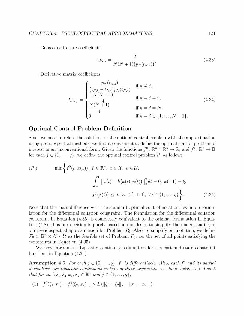
CHAPTER 4. PSEUDOSPECTRAL APPROXIMATIONS 124
Gauss quadrature coefficients:
ωN,k =2
N(N + 1)(pN(tN,k)
)2 . (4.33)
Derivative matrix coefficients:
dN,k,j =
pN(tN,k)(tN,k − tN,j
)pN(tN,j)
if k 6= j,
−N(N + 1)
4if k = j = 0,
N(N + 1)
4if k = j = N,
0 if k = j ∈ {1, . . . , N − 1}.
(4.34)
Optimal Control Problem Definition
Since we need to relate the solutions of the optimal control problem with the approximationusing pseudospectral methods, we find it convenient to define the optimal control problem ofinterest in an unconventional form. Given the functions f 0 : Rn×Rn → R, and f j : Rn → Rfor each j ∈ {1, . . . , q}, we define the optimal control problem P0 as follows:
(P0) min
{f 0(ξ, x(1)
)| ξ ∈ Rn, x ∈ X , u ∈ U ,∫ 1
−1
∥∥x(t)− h(x(t), u(t)
)∥∥2
2dt = 0, x(−1) = ξ,
f j(x(t)
)≤ 0, ∀t ∈ [−1, 1], ∀j ∈ {1, . . . , q}
}. (4.35)
Note that the main difference with the standard optimal control notation lies in our formu-lation for the differential equation constraint. The formulation for the differential equationconstraint in Equation (4.35) is completely equivalent to the original formulation in Equa-tion (4.8), thus our decision is purely based on our desire to simplify the understanding ofour pseudospectral approximation for Problem P0. Also, to simplify our notation, we defineF0 ⊂ Rn × X × U as the feasible set of Problem P0, i.e. the set of all points satisfying theconstraints in Equation (4.35).
We now introduce a Lipschitz continuity assumption for the cost and state constraintfunctions in Equation (4.35).
Assumption 4.6. For each j ∈ {0, . . . , q}, f j is differentiable. Also, each f j and its partialderivatives are Lipschitz continuous in both of their arguments, i.e. there exists L > 0 suchthat for each ξ1, ξ2, x1, x2 ∈ Rn and j ∈ {1, . . . , q},
(1) ‖f 0(ξ1, x1)− f 0(ξ2, x2)‖2 ≤ L (‖ξ1 − ξ2‖2 + ‖x1 − x2‖2).

CHAPTER 4. PSEUDOSPECTRAL APPROXIMATIONS 125
(2)∥∥∥∂f0∂ξ (ξ1, x1)− ∂f0
∂ξ(ξ2, x2)
∥∥∥2≤ L (‖ξ1 − ξ2‖2 + ‖x1 − x2‖2).
(3)∥∥∥∂f0∂x
(ξ1, x1)− ∂f0
∂x(ξ2, x2)
∥∥∥2≤ L (‖ξ1 − ξ2‖2 + ‖x1 − x2‖2).
(4) ‖f j(x1)− f j(x2)‖2 ≤ L ‖x1 − x2‖2.
(5)∥∥∥∂fj∂x (x1)− ∂fj
∂x(x2)
∥∥∥2≤ L ‖x1 − x2‖2.
We will restrict our analysis to problems where the minimum is achieved, and thereforethe feasible set is not empty. This condition is summarized in the following assumption.
Assumption 4.7. There exists a triple (ξ∗, x∗, u∗) ∈ F0 such that for each (ξ, x, u) ∈ F0,
f 0(ξ∗, x∗(1)
)≤ f 0
(ξ, x(1)
). (4.36)
Using the sets XN and UN , as defined in Equations (4.21) and (4.22), we can define thefollowing pseudospectral approximation of Problem P0. Let N ∈ N, {tN,k}Nk=0 a set of collo-
cation nodes as in Equation (4.16), and {ωN,k}Nk=0 its related Gauss quadrature coefficients,as defined in Equation (4.19). Moreover, let δ > 0, M =
⌈N4+δ
⌉, and {πk}∞k=0, a strictly
increasing divergent sequence. We define our pseudospectral approximation of Problem P0,as defined in Equation (4.35), as follows:
(PN,δ) min
{f 0(ξ, x(1)
)+πNε | ξ ∈ Rn, x ∈ XN , u ∈ UN , ε ∈ [0,∞),
M∑k=0
ωM,k
∥∥x(tM,k)− h(x(tM,k), u(tM,k)
)∥∥2
2≤(N−
δ3 + ε
)2,
x(−1) = ξ,
f j(x(tN,k)
)≤ N−
13 + ε, ∀k ∈ {0, . . . , N}, ∀j ∈ {1, . . . , q}
}(4.37)
Note that the time derivative of x ∈ XN in Equation (4.37), x, can be explicitly computedas explained in Equation (4.24). As we did with Problem P0, we define FN,δ ⊂ Rn×X ×U ×[0,∞) as the feasible set of Problem PN,δ, i.e. the set of all points satisfying the constraintsin Equation (4.37).
4.2 Global Minimizer Convergence of Pseudospectral
Approximations
In this section we show that for each δ > 0, every sequence of global minimizers of Prob-lems PN,δ, indexed by N ∈ N, accumulates in set of global minimizers of Problem P0.

CHAPTER 4. PSEUDOSPECTRAL APPROXIMATIONS 126
Feasibility of Pseudospectral Approximation
We begin with a lemma that provides useful estimates for the norm and total variation of asolution of Differential Equation (4.8) given its initial condition and control.
Lemma 4.8. There exists a constant C > 0 such that, for each tuple (ξ, x, u) ∈ F0:
(1) ‖x‖L∞ ≤ C(‖ξ‖2 + ‖u‖L2 + 1
),
(2) V(x) ≤ C(‖ξ‖2 + ‖u‖L2 + 1
),
where F0 is the feasible set of Problem P0, as defined in Equation (4.35).
Proof. Let t ∈ [−1, 1]. Then, by Differential Equation (4.8) and Condition 1 in Assump-tion 4.2,
‖x(t)‖2 ≤ ‖ξ‖2 + L
∫ 1
−1
(‖x(s)‖2 + ‖u(s)‖2 + 1
)ds. (4.38)
Thus, applying the Bellman-Gronwall Inequality (Lemma 5.6.4 in [Pol97]),
‖x(t)‖2 ≤ e2L(‖ξ‖2 + 2L ‖u‖L2 + 2L
), (4.39)
proving the inequality in Condition 1.The inequality in Condition 2 follows after noting that, by Theorem 4.1, and as we
computed in Equation (4.13) in the proof of Lemma 4.4:
V(x) =
∫ 1
−1
∥∥h(x(t), u(t))∥∥ dt ≤ √2L
(‖x‖L2 + ‖u‖L2 + 1
). (4.40)
Therefore, using Equation (4.39) we obtain the desired result.
The following lemma presents a rate of convergence for our polynomial approximationfor functions of bounded variation.
Lemma 4.9. There exists N0 ∈ N and C > 0 such that, for each f ∈ L2([−1, 1],R) ∩BV ([−1, 1],R), we can find a polynomial p of order N ≥ N0 satisfying:
‖f − p‖L2 ≤ C1√N
V(f) , (4.41)
where V(·) is as defined in Equation (4.5).
Proof. Our proof will be divided in two parts. First, we prove that we can approximatef using a trigonometric polynomial using a truncated Fourier series expansion. Then, weapproximate that trigonometric polynomial using its Taylor expansion.

CHAPTER 4. PSEUDOSPECTRAL APPROXIMATIONS 127
Let ck : [−1, 1] → R and sk : [−1, 1] → R by ck(t) = cos(2πkt) and sk(t) = sin(2πkt).Note that the set {ck, sk}∞k=1 forms an orthonormal basis for L2([−1, 1],R) using the dotproduct defined in Equation (4.2). Then, by Theorem 5.27 in [Fol99],
f = 〈f,1〉+∞∑k=1
〈f, ck〉 ck + 〈f, sk〉 sk. (4.42)
where 1 is the function identical to one for all t ∈ [−1, 1]. Let us define the truncated Fourierseries expansion of order M for f by:
SMf = 〈f,1〉+M∑k=1
〈f, ck〉 ck + 〈f, sk〉 sk. (4.43)
Now, using the identity in Equation (4.6),
|〈f, ck〉| =∣∣∣∣∫ 1
−1
f(t)1
2πksin(2πkt)dt
∣∣∣∣ ≤ 1
2πkV(f) , (4.44)
and using the same argument,
|〈f, sk〉| ≤1
2πkV(f) . (4.45)
Thus, by Parseval’s Identity (Theorem 5.27 in [Fol99]),
‖f − SMf‖2L2 =
∞∑k=M+1
|〈f, ck〉|2 + |〈f, sk〉|2
≤ 1
2π2V(f)2
∞∑k=M+1
1
k2
≤ 1
2π2V(f)2 1
M.
(4.46)
Let us now consider the Taylor expansion of order N for SMf at t = 0, denoted PN(SMf).By the Lagrange Remainder Formula (see Section 1.11.4 in [DR84] one of its expressions),
‖SMf − PN(SMf)‖L∞ ≤1
(N + 1)!
∣∣∣∣dN+1SMf
dtN+1(t′)
∣∣∣∣ ∣∣tN+1∣∣
≤ 1
(N + 1)!
∥∥∥∥dN+1SMf
dtN+1
∥∥∥∥L∞
(4.47)

CHAPTER 4. PSEUDOSPECTRAL APPROXIMATIONS 128
where we used the fact that∣∣tN+1
∣∣ ≤ 1 for each t ∈ [−1, 1], and t′ ∈ (−1, 1). But note that,using Equations (4.44) and (4.45),∣∣∣∣ dN+1
dtN+1(SMf)(t)
∣∣∣∣ =
∣∣∣∣∣M∑k=1
〈f, ck〉dN+1ckdtN+1
(t) + 〈f, sk〉dN+1skdtN+1
(t)
∣∣∣∣∣≤
M∑k=1
|〈f, ck〉| (2πk)N+1 + |〈f, sk〉| (2πk)N+1
≤ 2 V(f) (2π)NM∑k=1
kN
≤ 2 V(f) (2π)NMN+1.
(4.48)
Also, by Stirling’s Approximation (Equation (17.42) in [CT06]),
1
(N + 1)!<
1√2π(N + 1)
(e
N + 1
)N+1
. (4.49)
Hence, from Equations (4.47), (4.47), and (4.49) we know that there exists C ′ > 0 such that
‖SMf − PN(SMf)‖L2 ≤ C ′V(f)
(2πeM
N + 1
)N+1
. (4.50)
Finally, given N ≥ (3πe − 1), if we choose M =⌊N+13πe
⌋then by the Triangle Inequality
and Equations (4.46) and (4.50) we get the desired result.
Note that, from the proof of Lemma 4.9 we can conclude that a good estimate for N0 is25, which is important from an implementation point of view.
Besides providing a clear bound for the rate of convergence of polynomial approximationsto functions of bounded variation, Lemma 4.9 also proves that
⋃N∈NXN and
⋃N∈N UN are
dense in X and U , respectively. In particular, we get the following corollary.
Corollary 4.10. There exists C > 0 and N0 ∈ N such that, for each tuple (ξ, x, u) ∈ F0
and each N ∈ N, N ≥ N0, we can find a pair (xN , uN) ∈ XN × UN satisfying the followingconditions:
(1) ‖u− uN‖L2 ≤ C1√N
V(u),
(2) ‖x− xN‖X ≤ C1√N
(‖ξ‖2 + ‖u‖L2 + 1
),
where V(·) is as defined in Equation (4.5), and F0 is the feasible set of Problem P0, as definedin Equation (4.35).

CHAPTER 4. PSEUDOSPECTRAL APPROXIMATIONS 129
Proof. Since U ⊂ L2([−1, 1],Rm)∩BV ([−1, 1],Rm), then by Lemma 4.9 there exists uN ∈ UNthat satisfies the Condition (1).
Now, Lemma 4.4 indicates that x ∈ BV ([−1, 1],Rn). Hence, again using Lemma 4.9, foreach N ≥ N0 there exists C ′ > 0 and p ∈ XN−1 such that
‖x− p‖L2 ≤ C ′1√N
V(x) . (4.51)
Let xN ∈ XN defined by
xN(t) = ξ +
∫ t
−1
p(s)ds, (4.52)
where it is important to note that xN is indeed a polynomial or order at most N . Then,there exists C ′ > 0 such that for each t ∈ [−1, 1],
‖x(t)− xN(t)‖2 ≤∫ 1
−1
‖x(s)− p(s)‖2 ds ≤ C ′1√N
V(x) , (4.53)
where the last inequality follows by Holder’s Inequality. The conclusion follows from Equa-tions (4.51) and (4.53), the definition of the X -norm in Equation (4.15), and Condition 2 inLemma 4.8.
The following lemma states that given an element in the feasible set of Problem P0, wecan find an element in the feasible set of Problem PN,δ for N large enough.
Lemma 4.11. For each N ∈ N, let {tN,k}Nk=0 be the set of either Legendre–Gauss orLegendre–Gauss–Lobatto collocation nodes, as defined in Equations (4.27) and (4.31), re-spectively. Also, let {ωN,k}Nk=0 be its associated set of Gauss quadrature coefficients.
Then there exists C > 0 and N0 ∈ N such that, given (ξ, x, u) ∈ F0, N ≥ N0, and δ > 0,we can find (xN , uN) ∈ XN × UN satisfying:
(1)(∑M
k=0 ωM,k
∥∥xN(tM,k)− h(xN(tM,k), uN(tM,k)
)∥∥2
2
) 12 ≤ CN−
δ2
(‖ξ‖2+‖u‖L2+V(u)+1
),
(2) f j(xN(tN,k)
)≤ CN−
12
(‖ξ‖2 + ‖u‖L2 + 1
), ∀k ∈ {0, . . . , N}, ∀j ∈ {1, . . . , q},
where M =⌈N4+δ
⌉and V(·) is as defined in Equation (4.5).
Proof. LetN ≥ N0. Since x is feasible and f j is Lipschitz continuous, as stated in Condition 4in Assumption 4.6, there exists C1 > 0 such that for each j ∈ {1, . . . , q} and k ∈ {0, . . . , N}:
f j(xN(tN,k)
)≤∣∣f j(x(tN,k)
)− f j
(xN(tN,k)
)∣∣ ≤ C11√N
(‖ξ‖2 + ‖u‖L2 + 1
), (4.54)
where the last inequality follows by Condition 2 in Corollary 4.10.
CHAPTER 4. PSEUDOSPECTRAL APPROXIMATIONS 130
Let eN : [−1, 1] → Rn be defined by eN(t) = xN(t) − h(xN(t), uN(t)
). Then, by Condi-
tion 1 in Assumption 4.2 together with Condition 2 in Corollary 4.10, there exists C2 > 0such that:
‖eN‖L2 ≤ ‖xN − x‖L2 +
(∫ 1
−1
∥∥h(x(s), u(s))− h(xN(s), uN(s)
)∥∥2
2ds
) 12
≤ C11√N
(‖ξ‖2 + ‖u‖L2 + 1
)+ 2L
(‖x− xN‖L2 + ‖u− uN‖L2
)≤ C2
1√N
(‖ξ‖2 + ‖u‖L2 + V(u) + 1
).
(4.55)
Now let M ∈ N. Then, since the collocation nodes are either Legendre–Gauss or Legendre–Gauss–Lobatto, by Theorem 6.6.1 in [Fun92] we get that there exists C3 > 0 such that:
‖eN − IMeN‖L2 ≤ C31√M‖eN‖L2
≤ C31√M
(‖xN‖L2 +
∥∥∥∥dhdx∥∥∥∥L∞‖xN‖L2 +
∥∥∥∥dhdu∥∥∥∥L∞‖uN‖L2
).
(4.56)
In order to obtain a bound for the inequality in Equation (4.56) note that, by Condition 2in Corollary 4.10, Condition 1 in Assumption 4.2, and Lemma 4.8, there exists C4 such that:
‖xN‖L2 ≤ C11√N
(‖ξ‖2 + ‖u‖L2 + 1
)+ ‖x‖L2
≤ C4
(1√N
+ 1
)(‖ξ‖2 + ‖u‖L2 + 1
).
(4.57)
Also, note that by Condition 1 in Assumption 4.2:∥∥∥∥dhdx∥∥∥∥L∞≤ L, and
∥∥∥∥dhdu∥∥∥∥L∞≤ L, (4.58)
Moreover, Theorem 6.3.2 in [Fun92] states that there exists C4 > 0 such that for eachpolynomial p of order N :
‖p‖L2 ≤ C4N2 ‖p‖L2 . (4.59)
Therefore, from Equations (4.57), (4.58), and (4.59), we get the following estimate:
‖eN − IMeN‖L2 ≤ C5N2
√M
(‖ξ‖2 + ‖u‖L2 + V(u) + 1
), (4.60)
for some C5 > 0. The proof is complete by noting that there exists C6 > 0 such that:(M∑k=0
ωM,k ‖eN(tM,k)‖22
) 12
=
(M∑k=0
ωM,k ‖IMeN(tM,k)‖22
) 12
≤ C6 ‖IMeN‖L2 , (4.61)

CHAPTER 4. PSEUDOSPECTRAL APPROXIMATIONS 131
where the last inequality follows from Theorem 3.8.2 in [Fun92]. Therefore, using the boundsin Equations (4.55) and (4.60), we get that there exists C7 > 0 such that:(
M∑k=0
ωM,k ‖eN(tM,k)‖2
) 12
≤ C7
(1√N
+N2
√M
), (4.62)
thus, if we choose M =⌈N4+δ
⌉for any δ > 0, we get the desired result.
Now we can state the main result in this chapter, which is that global minimizers of anysequence of Problems PN,δ as N →∞,
Theorem 4.12. For each N ∈ N, let {tk}Nk=0 be a set of either Legendre–Gauss or Legendre–Gauss–Lobatto collocation nodes, as defined in Equations (4.27) and (4.31), respectively.Also, given δ > 0, let {(ξN , xN , uN , εN)}N∈N be a sequence of minimizers of Problems{PN,δ}N∈N, as defined in Equation (4.37).
Then any accumulation point of this sequence is of the form(ξ, x, u, 0
)∈ Rn ×X ×U ×
[0,∞), where the tuple(ξ, x, u
)is a minimizer of Problem P0, as defined in Equation (4.35).
Proof. Without loss of generality, let us assume that (ξN , xN , uN , εN) →(ξ, x, u, ε
). We
will first show that ε = 0. Recall that ε ≥ 0 since, by definition of the constraints ofProblem PN,δ, εN ≥ 0 for each N ∈ N.
Let us assume that ε > 0. Let(ξ, x, u
)∈ Rn × X × U be a minimizer of Problem (P0).
Then there exists a sequence{(ξN , xN , uN , εN
)}N∈N ⊂ FN,δ, where FN,δ is the feasible set
of Problem PN,δ, converging to(ξ, x, u, 0
). Indeed, for any C ′, δ′ > 0 there exists N0 such
that for each N ≥ N0:
C ′N−δ′2
(∥∥ξ∥∥2
+ ‖u‖L2 + V(u) + 1)≤ N−
δ′3 ,
C ′N−12
(∥∥ξ∥∥2
+ ‖u‖L2 + 1)≤ N−
13 .
(4.63)
Hence, by Lemma 4.11, for N ≥ N0 we can choose(ξN , xN , uN
)such that
(ξN , xN , uN , 0
)∈
FN,δ.Let α > 0, and let N1 ∈ N, N1 ≥ N0, such that for each N ≥ N1,
f 0(ξN , xN(1)
)≤ f 0
(ξ, x(1)
)+ α. (4.64)
Also, let N2 ∈ N, N2 ≥ N1, such that for each N ≥ N2
f 0(ξ, x(1)
)+ πN ε ≥ f 0
(ξ, x(1)
)+ 4α. (4.65)
Since the map (ξ, x) 7→ f 0(ξ, x(1)
)is continuous with the topology of Rn×X , there exists a
neighborhood V ⊂ Rn×X ×U × [0,∞) of(ξ, x, u, ε
)such that for each tuple (ξ, x, u, ε) ∈ V
f 0(ξ, x(1)
)+ πNε ≥ f 0
(ξ, x(1)
)+ 2α. (4.66)
CHAPTER 4. PSEUDOSPECTRAL APPROXIMATIONS 132
But we assumed that (ξN , xN , uN , εN) →(ξ, x, u, ε
), hence there exists N3 ∈ N, N3 ≥ N2,
such that (ξN , xN , uN , εN) ∈ V for each N ≥ N3. Thus:
f 0(ξN , xN(1)
)+ πN ε ≥ f 0
(ξ, x(1)
)+ 2α > f 0
(ξN , xN(1)
), (4.67)
which contradicts the fact that (ξN , xN , uN , εN) is a minimizer of Problem PN,δ. Thereforeε = 0.
Now we prove that(ξ, x, u
)is a minimizer of Problem P0. Suppose not, then:
f 0(ξ, x(1)
)< f 0
(ξ, x(1)
), (4.68)
and therefore, again by continuity of the map (ξ, x) 7→ f 0(ξ, x(1)
), there exists N4 ∈ N,
N4 ≥ N3, such that:f 0(ξN , xN(1)
)< f 0
(ξN , xN(1)
). (4.69)
Recall that εN = 0 for each N ≥ N4. Since (ξN , xN , uN , εN) is a minimizer of Problem PN,δ,then the following inequalities are satisfied:
f 0(ξN , xN(1)
)< f 0
(ξN , xN(1)
)+ πNεN ≤ f 0
(ξN , xN(1)
), (4.70)
but this is clearly a contradiction, hence proving the theorem.

133
Chapter 5
Conclusion
We have presented three results in the intersection of hybrid dynamical systems and optimalcontrol, with applications to Cyber–Physical Systems. The first result, in Chapter 2, isan algorithm that computes the optimal control of switched hybrid dynamical systems withstate constraints. The second result, in Chapter 3, is an algorithm that simulates autonomoushybrid dynamical systems using a novel relaxation technique. The third result, in Chapter 4,is an algorithm that computes the optimal control of nonlinear dynamical systems withstates constraints using pseudospectral approximations. These algorithms where developedmotivated by the some difficulties faced by Cyber–Physical applications, such as the problemof generalizing dynamical models to account for both continuous and discrete state variables,and the problem of improving the speed of computation so that large–scale problems can beaddressed.
Each of these results opens the doors to many research possibilities. First of all, we havenot tested any of these algorithms using experimental data. Algorithms tend to performbetter with simulated data than with experimental data, hence using them in real–life ap-plications is fundamental to understand their weaknesses. In particular, the algorithm inChapter 2 has many promising properties, as shown in Section 2.6, that make us think it willbe applicable to a wide range of applications. Second, in Chapter 3 we construct a hybridsystem metric, i.e. a metric that takes into account mode transitions to measure distanceswithin a hybrid dynamical system, which has the potential to solve many long standingproblems in hybrid system theory. Our result uses this hybrid system metric to prove thatour simulations converge to real trajectories, but at the same time it can be used to answerquestions about the topology of the hybrid system, such as finding the families of trajectoriesthat are not orbitally stable, or showing that some trajectories are Zeno. Also, we expect toextend our result on Chapter 3 to hybrid systems with controlled inputs, both continuousand discrete. Third, as explained in Chapter 4, our result in pseudospectral approximationsis just a first step towards finding an numerical method for the computation of optimalcontrol, based on pseudospectral methods, that can be provably convergent for practicalproblems. This is very relevant for real–life applications, since using this new algorithm willallow us to implement exciting experiments solving optimal control problems in real–time.

CHAPTER 5. CONCLUSION 134
Finally, we firmly believe that addressing the challenges faced today in the context ofCyber–Physical Systems will produce dramatic improvements to our society. The incor-poration of new distributed sources of energy to the electric power grid, autonomous carsthat guarantee our safety while increasing their performance, and the development of pros-thetic devices, are just a few of the applications where control theory for Cyber–PhysicalSystems plays a fundamental part. The results presented in this thesis are a small steptowards undertaking these huge problems, nevertheless we are certain that they are steps inthe right direction, and we hope that they help inspire even better results in the thrivingCyber–Physical research community.

135
Bibliography
[AA04] M. Alamir and S.-A. Attia, “On Solving Optimal Control Problems for Swit-ched Hybrid Nonlinear Systems by Strong Variations Algorithms,” in Proceedings of the6th IFAC Symposium on Nonlinear Control Systems, 2004, pp. 558–563.
[AA81] R. Alexander and S. Alexander, “Geodesics in Riemannian Manifolds–with–Boundary,” Indiana University Mathematics Journal, vol. 30, no. 4, pp. 481–488, 1981.
[AS05] A. D. Ames and S. S. Sastry, “A Homology Theory for Hybrid Systems: Hy-brid Homology,” in Proceedings of the 8th International Workshop on Hybrid Systems:Computation and Control, 2005, pp. 86–102.
[Axe+08] H. Axelsson, Y. Y. Wardi, M. Egerstedt, and E. I. Verriest, “GradientDescent Approach to Optimal Mode Scheduling in Hybrid Dynamical Systems,” Journalof Optimization Theory and Applications, vol. 136, no. 2, pp. 167–186, 2008.
[BBI01] D. Burago, Y. Burago, and S. Ivanov, A Course in Metric Geometry. Amer-ican Mathematical Society, 2001.
[BBM98] M. S. Branicky, V. S. Borkar, and S. K. Mitter, “A Unified Frame-work for Hybrid Control: Model and Optimal Control Theory,” IEEE Transactions onAutomatic Control, vol. 43, no. 1, pp. 31–45, 1998.
[BD05] S. C. Bengea and R. A. DeCarlo, “Optimal Control of Switching Systems,”Automatica, vol. 41, no. 1, pp. 11–27, 2005.
[Ben05] D. A. Benson, “A Gauss Pseudospectral Transcription for Optimal Control,”PhD thesis, Massachusetts Institute of Technology, 2005.
[Ber74] L. D. Berkovitz, Optimal Control Theory, ser. Applied Mathematical Sciences.Springer, 1974.
[Bet10] J. T. Betts, Practical Methods for Optimal Control and Estimation Using Non-linear Programming, 2nd ed. SIAM, 2010.
[Bro+02] B. Brogliato, A. A. ten Dam, L. Paoli, F. Genot, and M. Abadie, “Nu-merical Simulation of Finite Dimensional Multibody Nonsmooth Mechanical Systems,”Applied Mechanics Reviews, vol. 55, no. 2, pp. 107–150, 2002.
[Bro95] R. Brockett, “Stabilization of Motor Networks,” in Proceedings of the 34th IEEEConference on Decision and Control, 1995, pp. 1484–1488.
BIBLIOGRAPHY 136
[Bur+11] S. Burden, H. Gonzalez, R. Vasudevan, R. Bajcsy, and S. S. Sas-try, “Numerical Integration of Hybrid Dynamical Systems via Domain Relaxation,” inProceedings of the 50th Conference in Decision and Control, 2011, pp. 3958–3965.
[BV04] S. Boyd and L. Vandenberghe, Convex Optimization. Cambridge UniversityPress, 2004.
[Can+06] C. Canuto, M. Y. Hussaini, A. Quarteroni, and T. A. Zang, SpectralMethods: Fundamentals in Single Domains, ser. Scientific Computation. Springer, 2006.
[Can+88] C. Canuto, M. Y. Hussaini, A. Quarteroni, and T. A. Zang, SpectralMethods in Fluid Dynamics, 2nd ed., ser. Scientific Computation. Springer, 1988.
[Car78] M. B. Carver, “Efficient Integration Over Discontinuities in Ordinary Differen-tial Equation Simulations,” Mathematics and Computers in Simulation, vol. 20, no. 3,pp. 190–196, 1978.
[CCP70] M. D. Canon, C. D. Cullum, and E. Polak, Theory of Optimal Control andMathematical Programming. McGraw–Hill, 1970.
[CPW01] C. G. Cassandras, D. L. Pepyne, and Y. Y. Wardi, “Optimal Control ofa Class of Hybrid Systems,” IEEE Transactions on Automatic Control, vol. 46, no. 3,pp. 398–415, 2001.
[CT06] T. M. Cover and J. A. Thomas, Elements of Information Theory, 2nd ed. JohnWiley & Sons, 2006.
[DR84] P. J. Davis and P. Rabinowitz, Methods of Numerical Integration, 2nd ed.Academic Press, 1984.
[Dui+08] V. Duindam, R. Alterovitz, S. S. Sastry, and K. Goldberg, “Screw–Based Motion Planning for Bevel–Tip Flexible Needles in 3D Environments with Ob-stacles,” in Proceedings of the 2008 IEEE International Conference on Robotics andAutomation, 2008, pp. 2483–2488.
[EKP01] J. M. Esposito, V. Kumar, and G. J. Pappas, “Accurate Event Detectionfor Simulating Hybrid Systems,” in Proceedings of the 4th International Workshop onHybrid Systems: Computation and Control, 2001, pp. 204–217.
[EKR95] G. N. Elnagar, M. A. Kazemi, and M. Razzaghi, “The PseudospectralLegendre Method for Discretizing Optimal Control Problems,” IEEE Transactions onAutomatic Control, vol. 40, no. 10, pp. 1793–1796, 1995.
[ET87] I. Ekeland and R. Temam, Convex Analysis and Variational Problems. SIAM,1987.
[EW02] M. Egerstedt and Y. Y. Wardi, “Multi–Process Control Using Queuing The-ory,” in Proceedings of the 41st IEEE Conference on Decision and Control, 2002, pp. 1991–1996.

BIBLIOGRAPHY 137
[EWA06] M. Egerstedt, Y. Y. Wardi, and H. Axelsson, “Transition–Time Opti-mization for Switched–Mode Dynamical Systems,” IEEE Transactions on AutomaticControl, vol. 51, no. 1, pp. 110–115, 2006.
[FDF00] E. Frazzoli, M. A. Dahleh, and E. Feron, “Robust Hybrid Control forAutonomous Vehicle Motion Planning,” in Proceedings of the 39th IEEE Conference onDecision and Control, 2000, pp. 821–826.
[Fil88] A. F. Filippov, Differential Equations with Discontinuous Righthand Sides. KluwerAcademic Publishers, 1988.
[FL94] R. Fletcher and S. Leyffer, “Solving Mixed Integer Nonlinear Programs byOuter Approximation,” Mathematical Programming, vol. 66, no. 1, pp. 327–349, 1994.
[Fol99] G. Folland, Real Analysis: Modern Techniques and Their Applications, 2nd ed.,ser. Pure and Applied Mathematics. John Wiley & Sons, 1999.
[For96] B. Fornberg, A Practical Guide to Pseudospectral Methods, ser. Cambridge Mono-graphs on Applied and Computational Mathematics. Cambridge University Press, 1996.
[Fun92] D. Funaro, Polynomial Approximation of Differential Equations, ser. LectureNotes in Physics. Springer, 1992.
[Gil+11] J. H. Gillula, G. M. Hoffmann, H. Huang, M. P. Vitus, and C. J.Tomlin, “Applications of Hybrid Reachability Analysis to Robotic Aerial Vehicles,”The International Journal of Robotics Research, vol. 30, no. 3, pp. 335–354, 2011.
[GKR06] Q. Gong, W. Kang, and I. M. Ross, “A Pseudospectral Method for theOptimal Control of Constrained Feedback Linearizable Systems,” IEEE Transactionson Automatic Control, vol. 51, no. 7, pp. 1115–1129, 2006.
[Gon+07] Q. Gong, I. M. Ross, W. Kang, and F. Fahroo, “Connections Between theCovector Mapping Theorem and Convergence of Pseudospectral Methods for OptimalControl,” Computational Optimization and Applications, vol. 41, no. 3, pp. 307–335,2007.
[Gon+10a] H. Gonzalez, R. Vasudevan, M. Kamgarpour, S. S. Sastry, R. Ba-jcsy, and C. J. Tomlin, “A descent algorithm for the optimal control of constrainednonlinear switched dynamical systems,” in Proceedings of the 13th International Con-ference on Hybrid Systems: Computation and Control, 2010, pp. 51–60.
[Gon+10b] H. Gonzalez, R. Vasudevan, M. Kamgarpour, S. S. Sastry, R. Ba-jcsy, and C. J. Tomlin, “A numerical method for the optimal control of switchedsystems,” in Proceedings of the 49th IEEE Conference on Decision and Control, 2010,pp. 7519–7526.
[GT01] R. Ghosh and C. J. Tomlin, “Hybrid System Models of Biological Cell NetworkSignaling and Differentiation,” in Proceedings of the Annual Allerton Conference onCommunication Control and Computing, 2001, pp. 942–951.

BIBLIOGRAPHY 138
[Haa10] A. Haar, “Zur Theorie der Orthogonalen Funktionensysteme,” MathematischeAnnalen, vol. 69, no. 3, pp. 331–371, 1910.
[Hol99] K. Holmstrom, “The TOMLAB Optimization Environment in Matlab,” Ad-vanced Modeling and Optimization, vol. 1, no. 1, pp. 47–69, 1999.
[HR99] S. Hedlund and A. Rantzer, “Optimal Control of Hybrid Systems,” in Pro-ceedings of the 38th IEEE Conference on Decision and Control, 1999, pp. 3972–3977.
[HT11] T. Haberkorn and E. Trelat, “Convergence Results for Smooth Regulariza-tions of Hybrid Nonlinear Optimal Control Problems,” SIAM Journal on Control andOptimization, vol. 49, no. 4, pp. 1498–1522, 2011.
[Hun07] G. T. Huntington, “Advancement and Analysis of a Gauss Pseudospectral Tran-scription for Optimal Control Problems,” PhD thesis, Massachusetts Institute of Tech-nology, 2007.
[JEL99] K. H. Johansson, M. Egerstedt, and J. Lygeros, “On the regularizationof Zeno hybrid automata,” Systems & Control Letters, vol. 38, pp. 141–150, 1999.
[JM11] E. R. Johnson and T. D. Murphey, “Second–Order Switching Time Optimiza-tion for Nonlinear Time–Varying Dynamic Systems,” IEEE Transactions on AutomaticControl, vol. 56, no. 8, pp. 1953–1957, 2011.
[Kar84] N. Karmarkar, “A New Polynomial–Time Algorithm for Linear Programming,”Combinatorica, vol. 4, no. 4, pp. 373–395, 1984.
[KC07] V. Kallem and N. J. Cowan, “Image–guided Control of Flexible Bevel–TipNeedles.,” in Proceedings of the 2007 IEEE International Conference on Robotics andAutomation, 2007, pp. 3015–3020.
[KGR05] W. Kang, Q. Gong, and I. M. Ross, “Convergence of Pseudospectral Meth-ods for a Class of Discontinuous Optimal Control,” in Proceedings of the 44th IEEEConference on Decision and Control, 2005, pp. 2799–2804.
[KRG07] W. Kang, I. M. Ross, and Q. Gong, “Pseudospectral Optimal Control andIts Convergence Theorems,” in Analysis and Design of Nonlinear Control Systems: InHonor of Alberto Isidori, 2007, pp. 109–124.
[KZ05] A. J. Kurdila and M. Zabarankin, Convex Functional Analysis. Birkhauser,2005.
[Lee03] J. M. Lee, Introduction to Smooth Manifolds, ser. Graduate Texts in Mathematics.Springer, 2003.
[Lee97] J. M. Lee, Riemannian Manifolds: An Introduction to Curvature, ser. GraduateTexts in Mathematics. Springer, 1997.
[LR01] B. Lincoln and A. Rantzer, “Optimizing Linear System Switching,” in Pro-ceedings of the 40th IEEE Conference on Decision and Control, 2001, pp. 2063–2068.

BIBLIOGRAPHY 139
[Lyg+03] J. Lygeros, K. H. Johansson, S. N. Simic, J. Zhang, and S. S. Sastry,“Dynamical properties of hybrid automata,” IEEE Transactions on Automatic Control,vol. 48, no. 1, pp. 2–17, 2003.
[Lyg+99] J. Lygeros, K. H. Johansson, S. S. Sastry, and M. Egerstedt, “Onthe Existence of Executions of Hybrid Automata,” in Proceedings of the 38th IEEEConference on Decision and Control, 1999, pp. 2249–2254.
[Mal99] S. G. Mallat, A Wavelet Tour of Signal Processing. Elsevier, 1999.
[May+00] D. Q. Mayne, J. B. Rawlings, C. V. Rao, and P. O. M. Scokaert,“Constrained Model Predictive Control: Stability and Optimality,” Automatica, vol. 36,no. 6, pp. 789–814, 2000.
[MP75] D. Q. Mayne and E. Polak, “First–Order Strong Variation Algorithms forOptimal Control,” Journal of Optimization Theory and Applications, vol. 16, no. 3/4,pp. 277–301, 1975.
[OA09] Y. Or and A. D. Ames, “Formal and Practical Completion of Lagrangian HybridSystems,” in Proceedings of the 2009 American Control Conference, 2009, pp. 3624–3631.
[Pat68] T. N. L. Patterson, “On Some Gauss and Lobatto Integration Formulae,” Math-ematics of Computation, vol. 22, no. 104, pp. 877–881, 1968.
[Pic98] B. Piccoli, “Hybrid Systems and Optimal Control,” in Proceedings of the 37thIEEE Conference on Decision and Control, 1998, pp. 13–18.
[Pol97] E. Polak, Optimization: Algorithms and Consistent Approximation, ser. AppliedMathematical Sciences. Springer, 1997.
[Pon+62] L. S. Pontryagin, V. G. Boltyanskii, R. V. Gamkrelidze, and E. F.Mishchenko, The Mathematical Theory of Optimal Processes. Interscience Publishers,1962.
[PS03a] L. Paoli and M. Schatzman, “A Numerical Scheme for Impact Problems II: TheMultidimensional Case,” SIAM Journal on Numerical Analysis, vol. 40, no. 2, pp. 734–768, 2003.
[PS03b] L. Paoli and M. Schatzman, “A Numerical Scheme for Impact Problems I: TheOne–Dimensional Case,” SIAM Journal on Numerical Analysis, vol. 40, no. 2, pp. 702–733, 2003.
[PW84] E. Polak and Y. Y. Wardi, “A Study of Minimizing Sequences,” SIAM Journalon Control and Optimization, vol. 22, no. 4, pp. 599–609, 1984.
[RF03] I. M. Ross and F. Fahroo, “Legendre Pseudospectral Approximations of Opti-mal Control Problems,” in New Trends in Nonlinear Dynamics and Control and theirApplications, Springer, 2003, pp. 327–342.
[RF04] I. M. Ross and F. Fahroo, “Pseudospectral Knotting Methods for Solving Op-timal Control Problems,” Journal of Guidance, Control, and Dynamics, vol. 27, no. 3,pp. 397–405, 2004.

BIBLIOGRAPHY 140
[Rin+08] M. Rinehart, M. A. Dahleh, D. Reed, and I. V. Kolmanovsky, “Sub-optimal Control of Switched Systems With an Application to the DISC Engine,” IEEETransactions on Automatic Control, vol. 16, no. 2, pp. 189–201, 2008.
[Roc70] R. T. Rockafellar, Convex Analysis. Princeton University Press, 1970.
[RS04] H. Rehbinder and M. Sanfridson, “Scheduling of a Limited CommunicationChannel for Optimal Control,” Automatica, vol. 40, no. 3, pp. 491–500, Mar. 2004.
[Rud64] W. Rudin, Principles of Mathematical Analysis. McGraw–Hill, 1964.
[Rud91] W. Rudin, Functional Analysis, 2nd ed. McGraw–Hill, 1991.
[RW98] R. T. Rockafellar and R. J.-B. Wets, Variational Analysis, ser. Grundlehrender mathematischen Wissenschaften. Springer, 1998.
[RZL11] J. Ruths, A. Zlotnik, and S. Li, “Convergence of a Pseudospectral Method forOptimal Control of Complex Dynamical Systems,” in Proceedings of the 50th Conferencein Decision and Control, 2011, pp. 5553–5558.
[Sas99] S. S. Sastry, Nonlinear Systems: Analysis, Stability, and Control, ser. Interdisci-plinary Applied Mathematics. Springer, 1999.
[SB00] G. J. Sutton and R. R. Bitmead, “Performance and Computational Imple-mentation of Nonlinear Model Predictive Control on a Submarine,” in Nonlinear ModelPredictive Control, Birkhauser, 2000, ch. 3, pp. 461–472.
[SC03] M. S. Shaikh and P. E. Caines, “On the optimal control of hybrid systems:Optimization of trajectories, switching times, and location schedules,” in Proceedingsof the 6th International Workshop on Hybrid Systems: Computation and Control, 2003,pp. 466–481.
[SC07] M. S. Shaikh and P. E. Caines, “On the hybrid optimal control problem: theoryand algorithms,” IEEE Transactions on Automatic Control, vol. 52, no. 9, pp. 1587–1603,2007.
[SGB91] L. F. Shampine, I. Gladwell, and R. W. Brankin, “Reliable Solution ofSpecial Problems for ODEs,” ACM Transactions on Mathematical Software, vol. 17, no.1, pp. 11–25, 1991.
[Sim+05] S. N. Simic, K. H. Johansson, J. Lygeros, and S. S. Sastry, “Towards aGeometric Theory of Hybrid Systems,” Dynamics of Continuous Discrete and ImpulsiveSystems Series B: Applications & Algorithms, vol. 12, no. 5/6, pp. 649–688, 2005.
[SP96] A. Schwartz and E. Polak, “Consistent Approximations for Optimal ControlProblems Based on Runge–Kutta Integration,” SIAM Journal on Control and Optimiza-tion, vol. 34, no. 4, pp. 1235–1269, 1996.
[ST89] A. Solomonoff and E. Turkel, “Global Properties of Pseudospectral Meth-ods,” Journal of Computational Physics, vol. 81, no. 2, pp. 239–276, 1989.

BIBLIOGRAPHY 141
[Ste73] L. A. Steen, “Highlights in the History of Spectral Theory,” The American Math-ematical Monthly, vol. 80, no. 4, pp. 359–381, 1973.
[STW11] J. Shen, T. Tang, and L. Wang, Spectral Methods: Algorithms, Analysis andApplications, ser. Springer Series in Computational Mathematics. Springer, 2011.
[Sus72] H. J. Sussmann, “The “Bang-Bang” Problem for Certain Control Systems inGL(n,R),” SIAM Journal on Control and Optimization, vol. 10, no. 3, p. 470, 1972.
[Sus99a] H. J. Sussmann, “A Maximum Principle for Hybrid Optimal Control Problems,”in Proceedings of the 38th IEEE Conference on Decision and Control, 1999, pp. 425–430.
[Sus99b] H. J. Sussmann, “A Nonsmooth Hybrid Maximum Principle,” in Stability andStabilization of Nonlinear Systems, Springer, 1999, pp. 325–354.
[SW05] J. Shen and L. Wang, “Error Analysis for Mapped Legendre Spectral and Pseu-dospectral Methods,” SIAM Journal on Numerical Analysis, vol. 42, no. 1, pp. 326–349,2005.
[Tre12] E. Trelat, “Optimal Control and Applications to Aerospace: Some Results andChallenges,” Journal of Optimization Theory and Applications, vol. 154, no. 3, pp. 713–758, 2012.
[Vas+12] R. Vasudevan, H. Gonzalez, R. Bajcsy, and S. S. Sastry, “Consis-tent Approximations for the Optimal Control of Constrained Switched Systems,” 2012.arXiv:1208.0062v2.
[Vid02] M. Vidyasagar, Nonlinear Systems Analysis, 2nd ed., ser. Classics in AppliedMathematics. SIAM, 2002.
[WE12a] Y. Y. Wardi and M. Egerstedt, “Algorithm for Optimal Mode Schedulingin Switched Systems,” in Proceedings of the 2012 American Control Conference, 2012,pp. 4546–4551.
[WE12b] Y. Y. Wardi and M. Egerstedt, “Optimal Control of Autonomous Switched–Mode Systems: Conceptual and Implementable Algorithms,” Tech. Rep., 2012.
[WYB02] G. C. Walsh, H. Ye, and L. G. Bushnell, “Stability Analysis of NetworkedControl Systems,” IEEE Transactions on Control Systems Technology, vol. 10, no. 3,pp. 438–446, 2002.
[XA02] X. Xu and P. J. Antsaklis, “Optimal Control of Switched Autonomous Sys-tems,” in Proceedings of the 41st IEEE Conference on Decision and Control, vol. 4,IEEE, 2002, pp. 4401–4406.
[Zha+01] J. Zhang, K. H. Johansson, J. Lygeros, and S. S. Sastry, “Zeno HybridSystems,” International Journal of Robust and Nonlinear Control, vol. 11, no. 5, pp. 435–451, 2001.
[Zie89] W. P. Ziemer, Weakly Differentiable Functions, ser. Graduate Texts in Mathe-matics. Springer, 1989.