1

Computationally Efficient Trajectory Generation for

Fully-Actuated Multirotor VehiclesDario Brescianini, Student Member, IEEE, and Raffaello D’Andrea, Fellow, IEEE

Abstract—This paper presents a computationally efficientmethod of generating state-to-state trajectories for fully-actuatedmultirotor vehicles. The approach consists of computing trans-lational and rotational motion primitives that guide the vehiclefrom any initial state, defined by position, velocity and attitude,to any end state in a given time, and subsequently verifyingthe motion primitives’ feasibility. Computationally light-weightmotion primitives for which closed-form solutions exist are pre-sented and an efficient method to test their feasibility is derived.The algorithm is shown to be able to generate trajectories andverify their feasibility within a few microseconds and can thus beused as an implicit feedback law or in high level path plannersthat involve evaluating a large number of possible trajectoriesto achieve some high level goal. The algorithm’s performanceis analyzed by comparing it with time-optimal trajectories. Anexperimental demonstration that requires the computation oftrajectories for a large set of end states in real time is usedto evaluate the approach.

Index Terms—Trajectory generation, motion control, aerialrobotics.

I. INTRODUCTION

MULTIROTOR vehicles have become very popular aerial

robotic platforms due to their high maneuverability and

ability to hover. However, one of the limitations of traditional

multirotor vehicles is their inherent under-actuation, i.e. their

inability to independently control their thrust and torque in

all three dimensions. In order to increase performance criteria

such as flight duration or payload, all rotors are typically

arranged in a single plane, thereby limiting the thrust to a

single direction and coupling the vehicle’s translational and

rotational dynamics. This limits not only the set of feasible

trajectories, but also the vehicle’s ability to instantaneously

resist arbitrary force and torque disturbances as required when

flying high precision maneuvers or when physically interacting

with the environment. To overcome these limitations, several

novel multirotor vehicle designs with non-planar rotor config-

urations have been developed in the past years such as the

hexrotor vehicles [1]–[5] or the octorotor vehicle [6]. These

multirotor vehicles are capable of independently generating

thrust and torque in any direction and hence allow control of

all of their six degrees-of-freedom independently.

A. Goal and Motivation

A key feature required to exploit the full dynamic capabili-

ties of these novel multirotor vehicles is a trajectory generator

that can compute a large set of position and attitude flight paths

in real time while respecting the system dynamics and input

The authors are members of the Institute for Dynamic Systems and Control,ETH Zurich, Switzerland. {bdario, rdandrea}@ethz.ch

constraints. In many of the envisioned application areas such

as aerial manipulation or filming, the environment may con-

stantly change: the target object may move; large disturbances

may throw the vehicle off its originally planned course; or

information about the environment may only become available

in mid-flight. In such dynamic environments, pre-planned

trajectories may become suboptimal or even infeasible, and

thus a method to constantly adapt the trajectory in real time is

required. Furthermore, in many of these scenarios there exist

multiple trajectories which achieve the same high level goal

and hence a trajectory generator is needed which is capable

of rapidly evaluating a large set of trajectories and selecting

the best trajectory with respect to some performance measure.

B. Related Work

A number of trajectory generation algorithms for traditional

multirotor vehicles have been presented in recent years. These

algorithms can roughly be divided into three groups: A first

group of algorithms generates trajectories based on path prim-

itives, for example lines [7], polynomials [8], or splines [9],

and subsequently parametrizes the paths in time such that the

dynamic constraints are satisfied. A second group consists of

algorithms that make use of the differential flatness of the

system to approximate the input constraints by constraints on

position derivatives. Trajectories are then generated by solving

an optimal control problem on the translational kinematics

with the objective of, for example, minimizing the maneuver

duration [10] or some position derivatives [11], [12]. A compu-

tationally very inexpensive method of this group is presented

in [13], where the input constraints are neglected when solving

the optimization problem and an efficient method is used sub-

sequently to check whether the resulting trajectories violate the

input constraints. Finally, a third group of algorithms generates

trajectories by solving an optimal control problem on the full

system dynamics numerically, either leveraging Pontryagin’s

minimum principle [14] or using numerical optimal control

[15], [16].

Although the aforementioned algorithms can be used to

generate trajectories for the novel fully-actuated multirotor

vehicles, they do not take full advantage of the dynamic

capabilities of these vehicles as they only generate attitude

trajectories that are directly coupled with the vehicle’s position

trajectory. Some algorithms to generate decoupled position

and attitude trajectories have been developed for spacecraft

applications. For example in [17] and [18], trajectories are gen-

erated using separate position and attitude path primitives that

are then parametrized in time to ensure their feasibility with

respect to the input constraints. However, these algorithms are

2

usually not fast enough to apply in real time to multirotor

vehicles whose position and attitude control loops typically

run at rates of 50-100Hz [19], [20] and hence demand the

trajectories to be generated in a few milliseconds.

C. Contribution

This paper presents and analyzes a trajectory generation

algorithm for fully-actuated multirotor vehicles capable of

rapidly generating thousands of trajectories which guide the

vehicle from any initial state to any end state in a given time.

The algorithm is similar to the approach presented in [13]

and is based on concatenating computationally light-weight

motion primitives for which closed-form solutions exist. When

generating the motion primitives, the input constraints are

neglected and their feasibility is then validated a posteriori by

relating the motion primitives’ position and attitude trajectories

to the input constraints using the multirotor vehicle’s system

dynamics. In [13], only traditional multirotor vehicles with

planar rotor configurations were considered, i.e. vehicles that

can only produce a thrust in a single direction. For these aerial

vehicles, it is sufficient to only compute translational motion

primitives as this fully defines the vehicle’s state and control

inputs (up to a yaw rotation). However, this is not sufficient

for fully-actuated aerial vehicles and this paper thus presents

a method to generate both translational and rotational motion

primitives and introduces sufficient conditions to verify their

feasibility.

When computing the motion primitives, the vehicle’s ability

to control all of its six degrees of freedom independently is

used and separate motion primitives for the translational and

rotational motion are computed, each by solving an optimal

control problem. For the translational motion primitive, the

objective is to minimize the jerk, and for the rotational motion

primitive, the objective is to minimize the trajectory’s rotation

vector acceleration, an approximation of the angular acceler-

ation. In both cases, the solution trajectories are characterized

by polynomials in time, a key property that is used for the fast

and efficient validation of the trajectories’ feasibility.

Since the algorithm is able to generate trajectories for arbi-

trary initial states, final states and maneuver duration, it can

be applied to a large class of trajectory generation problems.

Furthermore, the algorithm is shown to be computationally

efficient and can generate approximately 500 000 trajectories

per second when implemented on a standard laptop computer.

Due to these two properties, the algorithm is well suited to be

used in high level path planners such as probabilistic roadmap

[21] or rapidly exploring random tree algorithms [22] that

involve evaluating large numbers of candidate trajectories, or

as an implicit feedback law similar to model predictive control

[23].

The algorithm’s performance is assessed through an experi-

mental demonstration that requires doing a search over a large

set of possible end states in real time. The goal is for a fully-

actuated multirotor vehicle to catch a thrown ball in a small

pouch. The trajectory generator is embedded in a high level

path planner that evaluates a set of possible end states such that

the ball is caught in the pouch. Because the ball’s flight path

varies for each throw, the trajectories cannot be pre-planned

and have to be generated in real time.

D. Outline

The remainder of this paper is organized as follows: Section

II introduces preliminaries on two attitude representations that

are used throughout the paper. In Section III, the system

dynamics and the input constraints of the multirotor vehicles

considered in this paper are presented. In Section IV, the

trajectory generation problem is formally stated. In Section

V, motion primitives that guide the vehicle from any initial to

any final state are introduced, and a method to determine their

feasibility is presented in Section VI. Section VII presents

a trajectory generation algorithm that fulfills the trajectory

generation problem. The algorithm’s performance compared

to the multirotor vehicle’s physical limits as well as results

on the computational costs are presented in Section VIII. An

experimental evaluation of the trajectory generation algorithm

is presented in Section IX, and the paper is concluded in

Section X.

II. PRELIMINARIES

In this section, two attitude representations that will be

used throughout the paper are introduced: the rotation vector

r ∈ R3 and the rotation matrix R ∈ SO(3), where SO(3)

denotes the Special Orthogonal Group, defined as

SO(3) = {R ∈ R3×3|RTR =RRT = I

and det(R) = 1},(1)

where I ∈ R3×3 is the identity matrix. The rotation matrix

representation is convenient for rotating vectors or expressing

the attitude kinematics. However, the constraints (1) on the

group of rotation matrices renders it difficult to use them

for attitude trajectory generation. Rotation vectors on the

contrary are an unconstrained three-parameter representation,

but rotating vectors or computing the attitude kinematics is

more complicated. For these reasons, the attitude trajectories in

this paper will be planned using rotation vectors, and rotation

matrices will be used to represent attitudes in all other cases. In

the following, the conversion between the two representations

and their relation to angular velocity is presented.

Any arbitrary rotation can be described by a rotation axis

and a rotation angle about this axis (see for example [24], and

references therein). Let n ∈ S2 be a unit vector which rep-

resents the axis of rotation, where S2 = {y ∈ R

3 | yTy = 1},

and let ϕ ∈ R be the rotation angle. The rotation vector r

describing this rotation is defined to be

r = ϕn. (2)

Note that the rotation vector representation is not unique. In

fact, any rotation vector r = ϕn+2kπn, with k any integer,

represents the same physical attitude. The rotation matrix R

corresponding to the physical attitude represented by r is given

by [24]

R = e[r], (3)

= I +sin ‖r‖‖r‖ [r] +

1− cos ‖r‖‖r‖2 [r]2, (4)

3

where ‖ · ‖ denotes the Euclidean norm√rTr and [r] is the

skew-symmetric cross-product matrix representation of r,

[r] =

0 −r3 r2r3 0 −r1−r2 r1 0

. (5)

Conversely, given a rotation matrix R, the rotation vector is

obtained by

[r] = logR, (6)

=ϕ

2 sinϕ

(

R −RT)

, (7)

where ϕ satisfies 1 + 2 cosϕ = trace(R) and ϕ ∈ [0, π].Let R(t) be a curve in SO(3) describing the attitude of a

rigid body relative to a fixed coordinate frame. The relation

between the angular velocity in body-fixed coordinates ω and

the rotation matrix and its temporal derivative is given by

[ω] = RTR. (8)

An analogous relation can be obtained when the attitude of a

body is described by a rotation vector r(t). Differentiating (4)

with respect to time and inserting it into (8) yields [24]

ω = W (r)r, (9)

where W (r) = I if ‖r‖ = 0, and otherwise

W (r) = I − 1− cos ‖r‖‖r‖2 [r] +

‖r‖ − sin ‖r‖‖r‖3 [r]2. (10)

III. DYNAMIC MODEL

In this section, the multirotor vehicle dynamics and its input

constraints are presented. Only fully-actuated multirotor vehi-

cles are considered, i.e. multirotor vehicles that can generate

thrust and torque in all three dimensions independently of

each other. For ease of notation, vectors may be expressed as

n-tuples x = (x1, x2, . . . , xn) with dimensions and stacking

clear from context.

A. Equations of Motion

The multirotor vehicle is modelled as a rigid body. The

translational degrees-of-freedom are described by the position

of the multirotor vehicle’s center of mass x = (x1, x2, x3),expressed in an inertial frame, and its rotational degrees-

of-freedom are parametrized using the rotation matrix

R ∈ SO(3).The multirotor vehicle’s control inputs are considered to

be the mass-normalized collective thrust f = (f1, f2, f3) and

the angular velocity ω = (ω1, ω2, ω3), both expressed in the

vehicle’s body-fixed coordinate frame as depicted in Fig. 1.

The thrust dynamics of multirotor vehicles are typically much

faster than their rigid body dynamics, and hence it is assumed

that the commanded thrust can be achieved instantaneously.

Likewise, it is assumed that the commanded angular veloc-

ity can be changed instantaneously. Because of multirotor

vehicles’ low rotational inertia and their ability to produce

large torques due to the off-center mounting of their rotors,

it is assumed that a high-bandwidth on-board controller can

track the angular velocity commands sufficiently fast using

x1 x2

x3

f

ω

g

Fig. 1: Illustration of a fully-actuated multirotor vehicle with its positiondescribed by x = (x1, x2, x3) in the inertial frame. The vehicle’s controlinputs are the mass-normalized collective thrust f and the angular velocityω. In addition, gravity g is acting upon the vehicle.

gyroscope feedback. The vehicle’s attitude dynamics are thus

neglected and the equations of motion can be written as

x = Rf − g, (11)

R = R[ω], (12)

where g is the acceleration due to gravity, expressed in the

inertial frame.

Note that more detailed models for the dynamics of multi-

rotor vehicles exist that incorporate, for example, aerodynamic

effects such as drag [25]. However, the preceding model

captures the most relevant dynamics and greatly simplifies the

trajectory generation problem, which then again allows com-

pensation for model inaccuracies by continuously re-planning

the trajectories. It should further be noted that by taking the

control inputs as the collective thrust and angular velocity,

the vehicle’s rotor configuration, i.e. the number of rotors,

their positions and orientations, is hidden from the equations

of motion by the on-board angular velocity controller that

computes the individual rotor thrusts based on the angular

velocity error and the commanded collective thrust. As a result,

the differential equations (11) and (12) describing the system

dynamics hold true for any fully-actuated multirotor vehicle,

such as the vehicles presented in [1]–[6].

B. Input Constraints

It is assumed that the control inputs are subject to satu-

rations. The attainable collective thrust is constrained to the

polyhedron

Aff � bf , (13)

where the symbol � denotes componentwise inequality. The

faces of the polyhedron described by (13) encode the thrust

limits in different directions that are due to the orientation

and saturation limits of the individual rotors. Examples of

attainable thrust volumes for fully-actuated multirotor vehicles

can be found in [4] and [5].

The angular velocity is assumed to be limited to the

polyhedron

Aωω � bω, (14)

4

where the limits can be due to, for example, the measurement

range of the gyroscope used for feedback or the range for

which the angular velocity controller responds sufficiently fast

to angular velocity commands such that the simplified system

dynamics (11) and (12) describe the system behaviour well.

An example of angular velocity constraints for the multirotor

vehicle [6] is given in Appendix A.

Without loss of generality, it is assumed in the following

that all rows of Af and Aω are unit vectors.

IV. PROBLEM STATEMENT

The trajectory generation problem addressed in this paper

can be formulated as follows: given an initial state at time

t = 0, consisting of position, velocity and attitude, find control

inputs f(t) and ω(t), t ∈ [0, T ], that steer the multirotor

vehicle to a desired final state at time t = T , while satisfying

the system dynamics (11) and (12) and input constraints (13)

and (14). Furthermore, the generation of trajectories should

be computationally inexpensive such that a large number of

trajectories can be computed in real time.

The approach presented in the following consists of two

steps: In a first step, motion primitives guiding the vehicle

from any initial to any desired end state in a given time

are planned while the input constraints are ignored. In a

second step, the control inputs are recovered from the motion

primitives’ position and attitude trajectory using the system

dynamics and then verified for input feasibility. If feasibility

cannot be established, the two steps are recursively performed

on subintervals and the resulting motion primitives are con-

catenated.

V. MOTION PRIMITIVE GENERATION

In this section, motion primitives that guide the multirotor

vehicle from any initial state to any desired end state in a

given time are presented. As in [13] for traditional multirotor

vehicles, the motion primitives are characterized by polynomi-

als in time. However, since fully-actuated multirotor vehicles

can independently control their position and attitude, it is not

sufficient to only compute a translational motion primitive

as for traditional multirotor vehicles, but a rotational motion

primitive also needs to be computed.

In the following, separate motion primitives for the vehicle’s

position and attitude are planned in the position coordinates

x and attitude coordinates r, respectively. It can be seen from

the system dynamics (11) and (12) that in order to be able

to recover the motion primitives’ corresponding control inputs

f(t) and ω(t), the position trajectory x(t) needs to be at

least twice differentiable with respect to time, and the attitude

trajectory r(t), or equivalently R(t), at least once. Without

loss of generality due to time invariance, the motion primitives

are planned on the interval [0, T ].

A. Translational Motion Primitive

The goal of the translational motion primitive is to guide the

vehicle from any initial position and velocity to any desired

end position and velocity in time T . We seek to find the motion

primitive that minimizes the average jerk squared on the time

interval [0, T ], i.e.

Jtrans =1

T

∫ T

0

‖...x(t)‖2dt. (15)

This cost function is chosen because it is computationally

convenient, a closed-form solution exists, and it works well

in practice. Furthermore, it yields a position trajectory that is

three times differentiable with respect to time. Consequently,

the corresponding control input f can be made continuous

even when concatenating multiple motion primitives and is

therefore easy to track.

The optimal jerk...x(t) minimizing (15) can be computed

using Pontryagin’s minimum principle (see for example [26])

and is derived in Appendix B. Its corresponding position,

velocity and acceleration trajectories can be shown to be of

the form

x(t) = c1

120 t5 + c2

24 t4 + c3

6 t3 + c4

2 t2 + c5t+ c6, (16)

x(t) = c1

24 t4 + c2

6 t3 + c3

2 t2 + c4t+ c5, (17)

x(t) = c1

6 t3 + c2

2 t2 + c3t+ c4. (18)

The constraints on the initial and final position and velocity

of the motion primitive only partially define the trajectories

(16)-(18). The motion primitive’s initial and final acceleration

can either be left free and subject to optimization, or they can

be used to ensure smooth transitions on the control input f

when concatenating multiple motion primitives by setting the

initial acceleration to be equal to the final acceleration of the

preceding motion primitive, and likewise for the final accel-

eration. If not mentioned otherwise, it will be assumed in the

remainder of this paper that also the initial and final acceler-

ation are defined, such that (x(0), x(0), x(0)) = (p0,v0,a0)and (x(T ), x(T ), x(T )) = (pT ,vT ,aT ). The components of

the coefficients c1, . . . , c6 along the i-th axis are then given

by

c1,ic2,ic3,i

=1

T 5

720 −360T 60T 2

−360T 168T 2 −24T 3

60T 2 −24T 3 3T 4

∆pi∆vi∆ai

, (19)

and

c4,ic5,ic6,i

=

a0,iv0,ip0,i

, (20)

where, for example, c1,i is the component of c1 along the i-thaxis and

∆pi∆vi∆ai

=

pT,i − p0,i − v0,iT − 12a0,iT

2

vT,i − v0,i − a0,iTaT,i − a0,i

. (21)

The cost of the motion primitive can then be computed to be

Jtrans =1

20cT1 c1T

4 +1

4cT1 c2T

3 +1

3

(

cT1 c3 + cT2 c2)

T 2

+ cT2 c3T + cT3 c3.(22)

5

B. Rotational Motion Primitive

The goal of the rotational motion primitive is to guide the

vehicle from any initial attitude to any desired end attitude in

time T . We seek to find the motion primitive that minimizes

the average rotation vector acceleration squared on the time

interval [0, T ], i.e.

Jrot =1

T

∫ T

0

‖r(t)‖2dt. (23)

Similar to the translational motion primitive, this cost function

is chosen because it is computationally convenient, has a

closed-form solution, works well in practice, and yields an

attitude trajectory that is twice differentiable with respect to

time. Consequently, the corresponding control input ω can

be made continuous and is thus easy to track even when

concatenating multiple motion primitives, which is exploited

in Section VII. In [27], it is shown that the rotation vector

acceleration r approaches the angular acceleration ω if either

• the rotation is small, i.e. ‖r(t)‖ → 0,

• the rotation is slow, i.e. ‖r(t)‖ → 0,

• or the rotation axis does not vary considerably, i.e.

∠(r, r) → 0 and ∠(r, r) → 0.

Minimizing the cost (23) can therefore be interpreted as an

approximation of minimizing the average angular acceleration

squared,

J =1

T

∫ T

0

‖ω(t)‖2dt, (24)

however, in general, the latter does not admit a closed-form

solution and is hence not well-suited to generate a large set

of trajectories in real time.

Let R0 and RT be the initial and final attitude, respectively.

In order to be able to compute the maximum rotation angle

in closed-form (see Section VI-A) and for the solution to

approximate the minimum angular acceleration trajectory well,

the motion primitive is always planned from an initial attitude

of r(0) = 0 to a final attitude of r(T ) = re such that ‖r(t)‖remains small, where re is the rotation between R0 and RT ,

[re] = log(RT0 RT ), (25)

and the resulting motion primitive is then rotated by R0 to

satisfy the original attitude conditions1.

As with the translational motion primitive, the optimal rota-

tion vector acceleration r(t) minimizing (23) can be computed

using Pontryagin’s minimum principle (see Appendix B for a

derivation) and yields attitude and angular velocity trajectories

of the form

R(t) = R0e[r(t)], (26)

ω(t) = W (r(t))r(t), (27)

1Note that (25) computes the rotation vector re such that ‖re‖ ≤ π,i.e. such that the rotation angle is smaller than π. By adding 2kπre/‖re‖ to(25), with k being any integer, the motion primitive ends at the same physicalattitude but performs an additional k full rotations. Throughout this paper, kis always chosen to be zero.

with

r(t) = d1

6 t3 + d2

2 t2 + d3t, (28)

r(t) = d1

2 t2 + d2t+ d3. (29)

Analogous to the translational motion primitive, the con-

straints on the initial and final attitude of the motion primitive

only partially define the attitude and angular velocity trajectory

(26)-(29). The initial and final angular velocity can either

be left free and subject to optimization, or they can be

used to ensure smooth transitions of the control input ω

when concatenating motion primitives by setting the initial

angular velocity to be equal to the final angular velocity

of the preceding motion primitive, and analogously for the

final angular velocity. If not mentioned otherwise, it will be

assumed in the remainder of this paper that the initial and final

angular velocity ω0 and ωT are also defined. The components

of the coefficients d1,d2 and d3 along the i-th axis are then

given by[

d1,id2,i

]

=1

T 3

[

−12 6T6T −2T 2

] [

re,i − ω0,iTωT,i − ω0,i

]

, (30)

and

d3,i = ω0,i, (31)

where ωT is defined to be

ωT := W−1(re)ωT . (32)

The cost of the motion primitive can then be shown to be

Jrot =1

3dT1 d1T

2 + dT1 d2T + dT

2 d2. (33)

C. Discussion

Generating the motion primitives can be done very effi-

ciently. In the case of the translational motion primitive, it

only requires the evaluation of (19) and (20) for each axis.

In the case of the rotational motion primitive, it requires the

evaluation of (25) and (32), and subsequently (30) and (31)

for each axis. In addition, calculating the costs of the motion

primitives is also computationally inexpensive and can be

done in closed-form using (22) and (33). If multiple motion

primitives achieve the same high level goal, these costs could

be used to compare the aggressiveness of the different motion

primitives.

VI. VERIFICATION OF FEASIBILITY

In this section a method to efficiently verify the motion

primitives’ feasibility is introduced. In [13], the feasibility

of the motion primitives was determined by finding extreme

points of the motion primitive’s position trajectory (and its

time derivatives) and relating them to the control input con-

straints using the differential flatness of traditional multirotor

vehicles. Due to the different system dynamics of fully-

actuated multirotor vehicles and the decoupled planning of

the translational and rotational motion primitive, the feasibility

checks of [13] cannot be applied to the motion primitives of

Section V and a different method to verify their feasibility is

devised.

6

Although the motion primitives for the position and attitude

are planned independently of each other, their feasibility can-

not be verified separately as the position and attitude dynamics

are coupled by the thrust input. The translational coordinates

are expressed in an inertial frame, but the thrust input and its

constraints are expressed in the vehicle’s body frame and hence

depend on the vehicle’s attitude. In the following, verifying the

motion primitives’ feasibility is done by first computing the

maximum rotation angle of the rotational motion primitive,

and then verifying whether the control inputs satisfy their

constraints under any rotation with a rotation angle equal or

smaller than the maximum rotation angle.

A. Maximum Rotation Angle

It can be seen from the multirotor vehicle’s attitude given in

(26) that the maximum rotation angle relative to the vehicle’s

initial attitude R0 is given by

ϕmax = max0≤t≤T

‖r(t)‖, (34)

and can be solved by finding the roots of

d

dt

(

rT (t)r(t))

= 0. (35)

By design of the rotational motion primitive, r(t) always has

one root at t = 0 and consequently (35) also has one root at

t = 0. Therefore, finding the other roots of (35) is equivalent

to finding the roots of a quartic polynomial, for which closed-

form solutions exist [28].

B. Thrust Input Feasibility

The thrust needed during the execution of the motion

primitives can be obtained through the translational dynamics

and is given by

f(t) = e[−r(t)]RT0 (x(t) + g) . (36)

The motion primitives’ feasibility with respect to the thrust

constraint, i.e.

Aff(t) � bf , ∀t ∈ [0, T ], (37)

is determined by first examining if the initial thrust is feasible,

AfRT0 (c4 + g) � bf , (38)

and afterwards verifying that the thrust remains feasible during

the entire motion primitive. This is done by computing a

bounding box on the required mass-normalized thrust, ex-

pressed in the vehicle’s initial body frame R0, and ensuring

that all points in the bounding box satisfy the thrust constraints

under any rotation with a maximum rotation angle of ϕmax.

Let H be the bounding box on the mass-normalized thrust

rotated into the vehicle’s initial body frame, i.e.

H = {y ∈ R3|hmin � R0y � hmax}, (39)

where the lower and upper bounds hmin and hmax are computed

such that

hmin � x(t) + g � hmax, ∀t ∈ [0, T ]. (40)

The lower and upper bounds are expressed in the inertial frame

for computational efficiency reasons (see Section VII) and are

obtained by evaluating x(t) at the boundaries of the interval

[0, T ] and by solving for the extrema of the acceleration x(t)along each axis on the interval [0, T ], which is essentially a

matter of finding the roots of its derivative (a polynomial of

order at most two).

The constraint (37) can then be formulated as

Afe[−r(t)]h � bf , ∀h ∈ H, ∀t ∈ [0, T ]. (41)

In Appendix C, it is shown that any point y ∈ R3 remains in

a closed ball B with center δfy and minimal radius ρf‖y‖under any rotation with a maximum rotation angle of ϕmax,

i.e.

e[−r(t)]y ∈ B (δfy, ρf‖y‖) , ∀t ∈ [0, T ], (42)

where

δf = cos(ϕ),

ρf = sin(ϕ),

ϕ = min[

ϕmax,π

2

]

.

(43)

Therefore, using (42), a sufficient condition for thrust feasi-

bility is

Af (δfh+ ρf‖h‖∆) � bf , ∀h ∈ H,

∀∆ ∈ B(0, 1),(44)

or equivalently (as all row vectors of Af are unit vectors)

Afδfh � bf − ρf‖h‖1, ∀h ∈ H, (45)

where 1 = (1, . . . , 1).Since the bounding box H is a convex set, every point in

H can be written as a convex combination of the vertices

of H. Furthermore, it is straightforward to verify that also

(45) describes a convex set and hence, for any two points

{h1,h2} ∈ H that satisfy (45), any convex combination

h = λh1 + (1− λ)h2, λ ∈ [0, 1] (46)

also satisfies (45). It is therefore sufficient to only validate that

the eight vertices of the bounding box H satisfy (45) in order

to guarantee feasibility with respect to the thrust input.

A visual interpretation of the thrust input feasibility check

is illustrated in Fig. 2.

C. Angular Velocity Input Feasibility

The angular velocity during the execution of the rotational

motion primitive is given in (27) and has to satisfy the

constraint

Aωω(t) � bω, ∀t ∈ [0, T ]. (47)

First, it is determined whether the initial angular velocity is

feasible, i.e.

Aωd3 � bω, (48)

and then it is verified that the angular velocity remains feasible

during the entire motion primitive by computing a bounding

box on the required rotation vector velocity and ensuring

7

O

t = 0 t = T

x(t) + g

(a)

OH

h

(b)

O

δfh

ρf‖h‖

(c)

Fig. 2: Visual interpretation of the thrust input feasibility check. Fig. 2(a) depicts the mass-normalized thrust trajectory x(t) + g during the time intervalt ∈ [0, T ]. If the initial thrust at t = 0 is found to be feasible, then a bounding box H on the required thrust is computed (see Fig. 2(b)). Because the thrustconstraint (13) is expressed in the vehicle’s body frame but the bounding box H is computed with respect to the vehicle’s initial body frame, i.e. the attitudeat t = 0, it needs to be verified that every point h ∈ H satisfies the thrust constraint when rotated into the vehicle’s body frame for any t ∈ [0, T ]. If ϕmax

denotes the maximum rotation angle of the rotational motion primitive during the interval [0, T ] relative to the vehicle’s initial attitude, then it can be shownthat any point y ∈ R3 remains in a closed ball with center δfy and minimal radius ρf‖y‖ under any rotation with a maximum rotation angle of ϕmax. Sincethe bounding box H is convex, it is sufficient to verify that the bounding balls of the eight vertices of H lie in the set of attainable thrusts (see Fig. 2(c)).

that all points in the bounding box satisfy the constraints

when mapped to angular velocities under any rotation with

a maximum rotation angle of ϕmax.

Let V describe the bounding box of the rotation vector

velocity,

V = {y ∈ R3 | vmin � y �vmax}, (49)

where the lower and upper bound vmin and vmax are computed

by finding the minimum and maximum of the rotation vector

velocity r(t) along each axis on the interval [0, T ]. This

involves evaluating r(t) at the boundaries of the interval and

at the root of its derivative (a linear polynomial).

The constraint (47) can then be rewritten as

AωW (r(t)) v � bω , ∀v ∈ V , ∀t ∈ [0, T ]. (50)

Similar to (42), it is shown in the Appendix C that any point

y ∈ R3 remains in a ball with center δωy and minimal radius

ρω‖y‖ under the map W (r(t))y for any rotation with a

maximum rotation angle of ϕmax, i.e.

W (r(t)) y ∈ B(δωy, ρω‖y‖), ∀t ∈ [0, T ], (51)

where

δω =

{

1, if ϕmax = 0,sin(ϕ)

ϕ, otherwise,

ρω =

{

0, if ϕmax = 0,1−cos(ϕ)

ϕ, otherwise,

ϕ = min[ϕmax, ϕ],

(52)

where ϕ is defined as the rotation angle at which the ball’s

radius is maximized,

ϕ := argmaxϕ>0

1− cos(ϕ)

ϕ. (53)

It therefore follows from (51) that a sufficient condition to

establish feasibility is

Aω (δωv + ρω‖v‖∆) � bω, ∀v ∈ V ,∀∆ ∈ B(0, 1),

(54)

or equivalently

Aωδωv � bω − ρω‖v‖1, ∀v ∈ V . (55)

As for the verification of the thrust feasibility, it is sufficient

to only verify that all vertices of the bounding box V satisfy

(55) in order to determine feasibility with respect to the

angular velocity input since both V and (55) are convex sets.

D. Discussion

The motion primitives’ feasibility can be tested at little

computational cost as it only involves verifying the feasibility

of a few distinct points, namely the vertices of the bounding

boxes H and V . Computing these vertices as well as computing

the maximum rotation angle only requires finding the roots of

a polynomial of order at most four and can therefore be done

in closed-form.

Furthermore, using the same methods as shown above,

the feasibility checks can easily be extended to handle state

constraints or further input constraints of the form

Ass(t) � bs (56)

or

AsR(t)s(t) � bs, (57)

where s(t) can be any state or control input trajectory (or

linear combinations thereof), as computing a bounding box

on these only involves finding the roots of at most a quartic

polynomial. The constraints (56) and (57) can be used, for

example, to encode boundaries on the vehicle’s position or

maximum angular velocity expressed in the inertial frame.

Due to the conservative approximations taken in the input

feasibility tests (45) and (55) by computing, for example,

bounding boxes, the input feasibility tests are sufficient but

not necessary. In particular, applying the input feasibility tests

can result in three possible outcomes. The motion primitives

can either be

• provably infeasible, if either (38) or (48) is false,

• provably feasible, if (45) and (55) hold true for all vertices

of the corresponding bounding box,

• or otherwise, their feasibility is indeterminable.

8

VII. TRAJECTORY GENERATION ALGORITHM

This section describes the trajectory generation algorithm

consisting of the previously derived motion primitives and

feasibility checks. First, a translational and rotational motion

primitive on the interval T = [τ1, τ2] = [0, T ] are planned

from a given initial state to a given final state. Afterwards,

the feasibility of the motion primitives, or more precisely of

the corresponding control input trajectories f(t) and ω(t), is

tested. If the feasibility tests return that the motion primitives

are either feasible or infeasible, the algorithm terminates

accordingly. If the feasibility could not be determined, the

time interval is split in half,

τ 1

2

=τ1 + τ2

2, (58)

T1 = [τ1, τ 1

2

], T2 = [τ 1

2

, τ2]. (59)

If the new interval length τ 1

2

− τ1 is below some threshold

τmin, the algorithm terminates without being able to gener-

ate a feasible trajectory. Otherwise, the algorithm is applied

recursively on the subinterval T1 to generate a trajectory

from the initial state s(τ1) to the final state s(τ 1

2

), where

s(t) = (x(t), x(t),R(t)) denotes the state trajectory corre-

sponding to the motion primitives computed on the interval

T . If the outcome is feasible, then the algorithm is also

applied recursively on the second subinterval T2 to generate

a trajectory from the initial state s(τ 1

2

) to the final state

s(τ2). If the outcome on the interval T2 is also feasible, the

motion primitives of the two intervals are concatenated and

the algorithm terminates with a proven feasible trajectory. In

addition to the initial state of the trajectory on T2 being equal

to the final state of the trajectory on T1, also the initial and

final acceleration and angular velocities on T2 and T1 are set to

be equal, in particular to x(τ 1

2

) and ω(τ 1

2

), in order to ensure

smooth transitions on the control inputs when concatenating

the motion primitives. The initial and final acceleration and

angular velocity on the interval T are chosen likewise and

are, for example, set to zero for rest-to-rest maneuvers.

Bisecting the time interval on which the trajectories are

generated is motivated by the conservative approximation of

the feasibility constraints. If the trajectory is planned on a

shorter time interval, the corresponding maximum rotation

angle will be smaller and the bounding boxes will be tighter,

hence reducing the conservativeness of the feasibility checks.

Note that due to the principle of optimality (see for example

[26]), the translational motion primitive only needs to be

computed once, as the optimal position trajectory x(t), t ∈ T ,

is also optimal on the subintervals t ∈ T1 and t ∈ T2, re-

spectively. When verifying the motion primitives’ feasibility,

the fact that the rotational motion primitive is planned from

r(0) = 0 is exploited in order to efficiently compute the

maximum rotation angle. However, this requires the nonlinear

transformations of the boundary conditions (25) and (32)

and as a consequence, the principle of optimality cannot

be applied to the rotational motion primitives. The optimal

attitude trajectory computed on a subinterval [τ1, τ2] ⊂ Tgenerally differs from the corresponding attitude trajectory

computed on the entire interval T , in particular if τ1 6= 0, and

PSfrag replacements

Time (s)

Angula

rvel

oci

ty(rad/s)

Rota

tion

vec

tor

(rad

)

0 T/2 T

− 2πT

0

2πT

−π2

0

π2

π

r1 r2 r3

ω1 ω2 ω3

Fig. 3: Attitude and angular velocity trajectories obtained by applying theproposed trajectory generation algorithm recursively on the interval [0, T ].The solid line represents the trajectories computed on the intervals [0, T ] and[0, T/2], respectively. The dashed line represents the trajectories computed onthe interval [T/2, T ]. For ease of interpretation, the rotation vector trajectoryon the interval[T/2, T ] is rotated by the attitude at t = T/2. It can beseen that the trajectories computed on the interval [T/2, T ] differ from thecorresponding trajectories computed on the entire time interval, despite havingthe same initial and final attitude and angular velocity.

therefore needs to be recomputed (see Fig. 3). As a result of

the changing attitude trajectories due to bisection, a trajectory

that is feasible but whose feasibility cannot be determined may

be rendered infeasible in a subsequent recursion step.

VIII. PERFORMANCE EVALUATION

This section attempts to assess the performance of the

proposed trajectory generation algorithm with respect to the

design objective of rapidly computing a large set of feasible

state-to-state trajectories for a given maneuver duration in real

time. If the trajectory generation algorithm finds a trajectory,

it is guaranteed to satisfy the system dynamics and input

constraints. However, if the algorithm is unable to find a

feasible trajectory, it does not imply that no feasible trajectory

exists, but could be due to

• the restriction of the trajectories to the motion primitives

of Section V (and concatenations thereof),

• or to the conservative approximations of the input con-

straints when verifying the feasibility, as the derived

feasibility conditions are only sufficient but not necessary

and therefore may require to perform a bisection step that

will render the trajectories infeasible.

In order to evaluate the conservativeness of the algorithm and

its applicability to real-time applications, its computational

costs when implemented on a standard laptop computer are

presented and a comparison with time-optimal trajectories is

given. The evaluations are carried out for a minimum time

interval length of τmin = 0.01s and for the omni-directional

octorotor vehicle presented in [6], whose thrust is constrained

9

PSfrag replacements

Relative minimum time duration

Per

centa

ge

of

traj

ecto

ries

0 0.1 0.2 0.3 0.4 0.5 0.6 0.7 0.8 0.9 10

5

10

15

20

25

Fig. 4: Comparison of the time-optimal maneuver duration relative to theshortest maneuver duration for which the presented algorithm is able to finda feasible trajectory. The comparison is carried out for 10 000 trajectoriesstarting from rest and steering the vehicle to randomized end states.

to a rhombic dodecahedron with an inradius of 19.6m/s2

and whose angular velocity components are constrained to

|ωi| ≤ 3rad/s, i ∈ {1, 2, 3} (see Appendix A for more de-

tails).

A. Computational Performance

In the following, the average computation time required to

run the algorithm on a standard laptop computer with an Intel

Core i7-3840QM CPU running at 2.8GHz, with 16GB of

RAM, is given. The algorithm was compiled with Microsoft

Visual C++ 14.0 and was run as a single thread application.

The average computation time was evaluated through gener-

ating one billion trajectories starting from rest at the origin

to randomized final states with maneuver durations drawn

uniformly at random between 0.25 s and 10.0 s. The vehicle’s

initial attitude was chosen such that its body frame is aligned

with the inertial frame. The final positions and velocities

were chosen uniformly at random from a box centered at the

origin with side lengths of 10m and 10m/s, respectively,

and the final attitudes where chosen uniformly at random

from SO(3). Since the maneuvers were planned from rest, the

initial acceleration and angular velocity were set to zero. The

components of the final acceleration and angular velocity were

chosen uniformly at random between −5m/s2 and 5m/s2,

and −1.5 rad/s and 1.5 rad/s, respectively.

The average computation time per trajectory, including

verifying its input feasibility, was measured to be 1.94 µs. Of

all computed trajectories, 86.3% were proven to be feasible,

10.9% were found to be infeasible, and the feasibility of

the remaining 2.8% could not be determined. Although the

algorithm was implemented on a laptop computer, modern

flight computers such as the Qualcomm Snapdragon Flight2

have similar specifications and the algorithm could therefore

also be run on board at a comparable rate.

The low computational cost of the proposed trajectory

generation algorithm can be exploited to rapidly search over a

large set of end states and maneuver durations that achieve

a certain high level goal, and to select the trajectory that

minimizes some high level cost.

2https://developer.qualcomm.com/hardware/snapdragon-flight

PSfrag replacements

Horizontal displacement (m)

Dura

tion

(s)

0 2 4 6 8 100

0.5

1

1.5

2

PSfrag replacements

Horizontal displacement (m)

Duration (s)

0

2

4

6

8

10

0

0.5

1

1.5

2

Fig. 5: The grey area represents the set of horizontal displacements along thex1-axis and end times for which feasible trajectories exist. This set was foundby computing the time-optimal maneuver numerically (solid line) and hence atrajectory longer than this always exists by simply waiting after executing thetime-optimal maneuver, but by definition no shorter trajectory exists (whitearea). The dashed line indicates the shortest maneuver durations for whichthe algorithm was able to generate a feasible trajectory.

B. Comparison with Time-Optimal Trajectories

Consider the motion primitives of Section V that guide the

vehicle from an initial state to a desired end state in time T . As

the maneuver duration is increased, T → ∞, it can be derived

from (19) and (30) that the motion primitives’ coefficients c1,

c2, c3, d1 and d2 converge to zero. The vehicle’s required

control inputs f(t) and ω(t) therefore converge to

limT→∞

f(t) = e[−ω0t]RT0 (a0 + g) , (60)

limT→∞

ω(t) = ω0. (61)

The initial acceleration a0 and angular velocity ω0 are design

parameters that can be chosen arbitrarily. The algorithm is

therefore guaranteed to find a feasible trajectory for sufficiently

long maneuver durations if the multirotor vehicle can generate

sufficient thrust in any direction to overcome gravity g, as for

example the multirotor vehicles [5], [6]. In order to quantify

the algorithm’s conservatism, the minimum maneuver duration

for which the algorithm can find a feasible trajectory is

compared with the duration of the time-optimal maneuver.

The time-optimal trajectories are computed using GPOPS-

II [29], a numerical optimal control software, and the fastest

trajectory found by the proposed algorithm is used as initial

guess for the time-optimal maneuver. Fig. 4 shows the result

of a comparison for 10 000 maneuvers starting from rest at

the origin and with the vehicle’s body frame aligned with the

inertial frame to final states drawn uniformly at random from

the set described in Section VIII-A. On average, the time-

optimal maneuver duration is 33.8% faster than the shortest

maneuver for which the presented algorithm is able to find a

feasible trajectory3.

A comparison of the maneuver durations for pure rest-to-

rest horizontal translations along the x1-axis with the initial

and final body frame aligned with the inertial frame is given in

3A bisection method was used to determine the shortest maneuver durationfor which the presented trajectory generation algorithm is able to find afeasible trajectory. Computing the shortest maneuver duration using bisectiontook on average less than one millisecond (bisection was terminated whenthe bisection interval size was smaller than one millisecond), while GPOPS-II took between several minutes and an hour to compute a solution.

10

Fig. 5. The time-optimal maneuvers are on the order of 20%

faster than the fastest feasible trajectories generated by the

proposed algorithm. This is due to limiting the trajectories to

the motion primitives of Section V, but also to the decoupled

planning of the motion primitives. An analysis of the time-

optimal maneuvers revealed that it is beneficial for the vehicle

to rotate in order to accelerate faster and hence reach the target

position quicker, even though the initial and final attitude are

identical.

IX. EXPERIMENTAL RESULTS

This section presents an experiment to verify the feasibility

of the trajectory generation algorithm for real-time applica-

tions that require the evaluation of a large set of possible

trajectories. The goal is for a fully-actuated multirotor vehicle

to catch a ball thrown by a person in a small pouch. This task

was chosen because a large number of trajectories exist that

achieve the goal and need to be evaluated in real time, and is

therefore well suited to test the algorithm’s speed and assess

its performance experimentally.

The experiments were carried out in the Flying Machine

Arena [20], an indoor aerial vehicle test bed at ETH Zurich,

using the omni-directional octorotor vehicle [6]. An overhead

motion-capture system provides position and attitude informa-

tion of the vehicle and the ball. This information is processed

on a desktop computer that estimates the state of the vehicle

and the ball, plans a catching maneuver accordingly and sends

out control commands to the vehicle through a low-latency

radio link at a rate of 50Hz. In order to be able to catch the

ball, the octorotor vehicle is equipped with a pouch of radius

5.75 cm at a distance of 47.5 cm from the vehicle’s center

of mass (see Fig. 6). A table tennis ball, modelled as a point

mass with aerodynamic drag proportional to its speed squared,

is used in the experiments. All results shown in the following

are from actual flight experiments.

Fig. 6: Omni-directional octorotor vehicle equipped with a pouch. The pouchis used to catch a thrown ball and thereby demonstrating the algorithm’sperformance experimentally.

PSfrag replacements

Horizontal position (m)V

erti

cal

posi

tion

(m)

0 0.5 1 1.5 2 2.5 3

−0.5

0

0.5

−0.5

0

0.5

−0.5

0

0.5

PSfrag replacements

Horizontal position (m)

Vertical position (m)

0

0.5

1

1.5

2

2.5

3

−0.5

0

0.5

−0.5

0

0.5

−0.5

0

0.5

Fig. 7: Three candidate catching maneuvers that guide the octorotor vehiclefrom rest to a state in which the ball is caught in the pouch. The dashed linerepresents the predicted ball flight path, and the goal is to catch the ball at aheight of zero meters. The maneuver shown in the top plot was found to bethe feasible maneuver with the lowest cost, and the maneuver on the bottomwas found to be infeasible.

A. High Level Path Planner

The trajectory generation algorithm is embedded in a high

level path planner that performs a brute-force search over a

set of possible catching and stopping maneuvers and selects

the maneuvers with the lowest cost.

1) Catching Maneuver: As soon as the ball is thrown into

the air, its catching position and flight duration is predicted

and a catching maneuver is planned using the current vehicle

state as initial condition and with free initial acceleration and

angular velocity (see Appendix B). The catching position is

defined to be the position where the ball crosses a fixed height.

The vehicle’s state at the end of the catching maneuver is

chosen such that the pouch is at the catching position and

that its normal direction points in the opposite direction of the

ball’s velocity. In addition, the ball is caught with the pouch at

rest except for an angular velocity about its normal direction

in order to be less prone to timing errors. A brute-force search

over 1600 end states is performed, in particular over

• 40 final positions, equally spaced around the ball’s catch-

ing position,

• and 40 final angular velocities, equally spaced between

±3 rad/s and with the vehicle’s velocity and acceleration

set accordingly such that the pouch remains at rest.

Fig. 7 shows three of the possible 1600 catching maneuvers

that are evaluated for an initial prediction of the ball’s flight

path.

11

PSfrag replacements

Time (s)

Angula

rvel

oci

ty(rad/s)

Thru

st(m/s2)

Position x1

(m)

Positionx2

(m)

Posi

tionx3

(m)

0 0.5 1 1.368 1.5 2 2.5 2.868−1

0

1

2

3

− 3π4

−π2

−π4

0

π4

−5

0

5

10

15

−1

0

1

0

1

2

3

f1 f2 f3

ω1 ω2 ω3

PSfrag replacements

Time (s)

Angular velocity (rad/s)

Thrust(m/s2

)

Position x1 (m)

Position x2 (m)

Position x3 (m)

0

0.5

1

1.368

1.5

2

2.5

2.868

−1

0

1

2

3

− 3π4

−π2

−π4

0π4

−5

0

5

10

15

−1

0

1

0

1

2

3

f1

f2

f3

ω1

ω2

ω3

Fig. 8: The left hand side shows a complete catching and stopping maneuver. The dashed line denotes the ball’s flight path. After the ball is first detected, thevehicle has 1.368 s time to move the pouch to the catching position starting from rest. Snapshots of the catching maneuver are depicted at the time instancest = {0 s, 0.62 s, 0.96 s, 1.368 s, 1.82 s, 2.868 s}. During the catching maneuver, the octorotor vehicle translated 2.25m and rotated 72.2◦, and had a finalangular velocity of −2.38 rad/s at the time of catching. The right hand side shows the respective control inputs. Note that the control inputs during thecatching maneuver do not represent a single catching trajectory but are the result of constantly re-planning the catching maneuver at each controller updatestep.

The feasibility of the trajectories is verified with respect to

the vehicle’s input constraints as introduced in Section VIII

and presented in more detail in Appendix A. Furthermore, a

box constraint on the position using (56) was implemented to

ensure that the vehicle remains within a safe flying space.

From all feasible catching maneuvers for which also a

stopping maneuver exists, the catching maneuver with the

lowest cost

Jtrans + αJrot (62)

is selected, where Jtrans and Jrot are the sums of the transla-

tional and rotational costs (22) and (33) over all concatenated

motion primitives. The design parameter α describes a trade-

off between translational and rotational costs and is set to

α = 10 in the experiments.

2) Stopping Maneuver: Using the final state of the catch-

ing maneuver as initial condition, a stopping maneuver is

planned that guides the vehicle to rest with free final position

and attitude. The adapted translational and rotational motion

primitive with the final position and attitude being subject to

optimization are given in Appendix B. A brute-force search

over five trajectories with a maneuver duration equally spaced

between 0.5 s and 1.5 s is performed and the feasible stopping

maneuver with the lowest cost (62) is selected.

B. Control Strategy

During the catching maneuver, the output of the high level

path planner is applied as an implicit feedback law. At each

controller update step, i.e. every 20ms, the prediction of the

catching position and the remaining flight duration is refined

using the most recent motion capture data. The catching

maneuver is then re-planned starting from the vehicle’s current

state by evaluating a maximum of 8000 (40 × 40 × 5) trajec-

tories and the initial control inputs f and ω corresponding to

the feasible catching maneuver with the lowest cost are sent

to the vehicle. If no feasible trajectory can be found, then

the last found feasible trajectory is tracked using the feedback

controller presented in [6]. The same feedback controller is

also used to track the stopping maneuver.

C. Results

The full catching and stopping maneuver for the same throw

as shown in Fig. 7 is depicted in Fig. 8. The ball’s flight lasted

1.368 s, during which the vehicle started from rest and covered

a distance of 2.25m and rotated 72.2◦ in order to catch

the ball. The catching maneuver is similar to the maneuver

shown in the top plot of Fig. 7 for the initial prediction

of the ball’s flight path, but is continuously re-planned as

new pose information of the vehicle and the ball become

available. During the catching maneuver, a total of 120 785

trajectories were computed, 110 400 catching maneuvers and

10 385 stopping maneuvers.

A video showing the vehicle catching the ball is

attached to the paper and can also be accessed on

https://youtu.be/0gR1ekapOAE.

12

X. CONCLUSION

This paper presented and analyzed a computationally ef-

ficient method for the rapid generation and feasibility veri-

fication of trajectories that guide a fully-actuated multirotor

vehicle from any initial to any desired end state in a given time.

The algorithm is based on recursively generating state-to-state

motion primitives and subsequently verifying their feasibility.

Computationally inexpensive motion primitives for the vehi-

cle’s position and attitude were derived that are characterized

by polynomials in time. This allowed for efficiently comput-

ing bounds on the vehicle’s acceleration, rotation angle and

rotation vector velocity, which were then used to verify the

motion primitives’ feasibility. A trajectory generation algo-

rithm based on the derived motion primitives and feasibility

tests was introduced. If the feasibility of a motion primitive

cannot be determined due to the conservative approximation of

the constraints, the trajectory generation algorithm is applied

recursively on subintervals and the resulting motion primitives

are concatenated.

The algorithm’s computational efficiency and speed is due

to the restriction of the trajectories to certain motion primitives

for which closed-form solutions exist and due to the conser-

vative approximation of the input constraints when testing the

feasibility. However, this comes at the expense of not always

being able to find a feasible trajectory for a given initial and

final state and maneuver duration although a feasible trajectory

exists. In order to characterize its performance and assess its

conservativeness, the trajectories generated by the algorithm

were compared with time-optimal maneuvers.

The feasibility of the algorithm for real-time applications

that require the evaluation of large numbers of trajectories was

verified experimentally by catching a ball thrown by a person

with a small pouch attached to an omni-directional octorotor

vehicle. For this purpose, the algorithm was embedded in a

high level path planner that performed a brute-force search

over a large number of candidate trajectories and selected

the maneuver with the lowest cost. In order to cope with

disturbances and changing final states, the trajectory planning

was repeated at each controller update step with the vehicle’s

current state as initial condition, and the output trajectory was

then applied as an implicit feedback law.

While the presented method allows for generating state-

to-state trajectories for any fully-actuated multirotor vehicle,

it is only guaranteed to find a feasible trajectory for an

infinitely large maneuver duration if the vehicle is able to

hover at any attitude. This is due to the decoupled planning of

the translational and rotational motion primitives which does

not take the input constraints into account. Considering the

algorithm’s speed, one approach to overcome this limitation

could be to embed the trajectory generation algorithm in a

high level path planner such as a rapidly exploring random

tree algorithm in order to to explore different attitude paths

and find feasible trajectories.

APPENDIX A

OCTOROTOR VEHICLE INPUT CONSTRAINTS

This appendix presents the input constraints of the omni-

directional octorotor vehicle presented in [6] that is used in

this paper as an example fully-actuated multirotor vehicle to

evaluate the performance of the trajectory generation algorithm

as well as for the experimental results.

The octorotor vehicle uses reversible fixed-pitch rotors that

can produce both positive and negative thrust. Each single

rotor thrust is subject to the saturation limits

−fmax ≤ frot ≤ fmax. (63)

If the aerodynamic interference between rotors is neglected,

the collective thrust f and torque t produced by the eight

rotors can be written as

[

f

t

]

=

[

n1 . . . n8

p1 ×n1 + κn1 . . . p8 ×n8 + κn8

]

︸ ︷︷ ︸=:B

frot,1

...

frot,8

, (64)

where frot,i is the thrust magnitude generated by the i-th rotor,

ni is the rotor disk normal, pi is the rotor position relative

to the vehicle’s center of mass and κ is the rotor’s specific

thrust-to-drag ratio. The exact numerical values of the rotor

configuration can be found in [6]. The set of attainable thrusts

and torques can be written as

{Bfrot ∈ R6 | frot ∈ R

8, ‖frot‖∞ ≤ fmax}. (65)

Applying the method presented in [30], the set of attainable

thrusts and torques (65) can be described by a polyhedron of

the form

[

Af Aτ

]

[

f

t

]

� b. (66)

A slice through this polyhedron at t = 0 then yields the set

of attainable thrusts when producing zero torque

Aff � b, (67)

and can be further simplified by removing all redundant

inequalities, resulting in the rhombic dodecahedron

Aff � bf , (68)

with

Af =1

2

−2 0 0

−1 1√2

−1 1 −√2

−1 −1√2

−1 −1 −√2

0 −2 00 2 01 1

√2

1 1 −√2

1 −1√2

1 −1 −√2

2 0 0

[

cos(

π12

)− sin

(π12

)0

sin(

π12

)cos

(π12

)0

0 0 1

]

, (69)

bf = fmax

√

32

31. (70)

The set of attainable thrusts (68) for a mass-normalized

maximum rotor thrust of fmax = 6m/s2 is illustrated in Fig.

9.

Rotating the octorotor vehicle while maintaining a thrust

in the same inertial direction typically requires some rotors

to change their spinning direction. However, reversing the

spinning direction of too many motors in rapid succession

13

PSfrag replacements

f1(m/s

2)

f2 (

m/s 2 )

f3

(m/s2)

−20−10

010

20

−20−10

010

20

−20

−10

0

10

20

Fig. 9: Rhombic dodecahedron with an inradius of 19.6m/s2 describing theset of attainable thrusts for the octorotor vehicle presented in [6].

can cause instabilities. Experiments revealed that the low-order

dynamic model with angular velocity as the control input

approximates well the true system dynamics for an angular

velocity of up to ωmax = 3 rad/s per axis. The angular velocity

of the vehicle is thus constraint to the box

Aωω � bω, (71)

with

Aω =

1 0 0−1 0 00 1 00 −1 00 0 10 0 −1

, (72)

bω = ωmax1. (73)

APPENDIX B

DERIVATION OF MOTION PRIMITIVES

This appendix presents the derivations of the translational

and rotational motion primitive introduced in Section V. The

motion primitives’ trajectories are computed using Pontrya-

gin’s minimum principle and solutions are provided for the

different initial and final conditions used in this paper.

A. Translational Motion Primitive

We seek to find the motion primitive that minimizes the cost

Jtrans =1

T

∫ T

0

‖...x(t)‖2dt. (74)

The optimal jerk...x(t) minimizing (74) can be computed for

each axis individually as the total cost is simply the sum of

the costs along each axis,

Jtrans =

3∑

i=1

Jtrans,i =

3∑

i=1

1

T

∫ T

0

...x2i (t)dt. (75)

In the following, the solution along the xi-direction,

i ∈ {1, 2, 3}, is derived. For the sake of readability, the

subscript i is omitted in the following and, for example,

the scalar x denotes xi, i.e. the i-th component of x. Let

s = (s1, s2, s3) = (x, x, x) be the state and u =...x be the

input. The Hamiltonian is then defined by

H(s, u,λ) =1

Tu2 + λ1s2 + λ2s3 + λ3u, (76)

where λ are the adjoint variables that must satisfy

λ = −∇sH(s, u,λ) = (0,−λ1,−λ2) . (77)

The result of the adjoint differential equation is

λ1(t) = − 1

T2c1, (78)

λ2(t) =1

T(2c1t+ 2c2), (79)

λ3(t) =1

T(−c1t

2 − 2c2t− 2c3). (80)

The optimal control u∗ that minimizes the cost function is

obtained by

u∗(t) = argminu

H(s, u,λ), (81)

=c12t2 + c2t+ c3, (82)

with the corresponding optimal state trajectories

s∗1(t) =c1120 t

5 + c224 t

4 + c36 t

3 + c42 t

2 + c5t+ c6, (83)

s∗2(t) =c124 t

4 + c26 t

3 + c32 t

2 + c4t+ c5, (84)

s∗3(t) =c16 t

3 + c22 t

2 + c3t+ c4. (85)

Although Pontryagin’s minimum principle is only a necessary

condition for optimality, it can be shown that u∗ indeed

minimizes (74) by exploiting the fact that the state dynamics

are linear and the cost is convex [31].

If the initial and final state are fully defined, i.e.

s(0) = (p0, v0, a0) and s(T ) = (pT , vT , aT ), the coefficients

c1, . . . , c6 can be determined by evaluating the optimal state

trajectory s∗(t) at time t = 0,

c4c5c6

=

a0v0p0

, (86)

and at time t = T ,

c1c2c3

=1

T 5

720 −360T 60T 2

−360T 168T 2 −24T 3

60T 2 −24T 3 3T 4

∆p∆v∆a

, (87)

where

∆p∆v∆a

=

pT − p0 − v0T − 12a0T

2

vT − v0 − a0TaT − a0

. (88)

14

By combining the optimal state trajectories (83)-(85) of each

axis, the translational motion primitive’s position, velocity and

acceleration trajectory (16)-(18) are obtained.

If a component of the initial or final state is left free and

subject to optimization, then its corresponding adjoint variable

must be equal to zero at time t = 0 or t = T , respectively.

The solutions for the different boundary conditions used in this

paper are given in the following. In any case, the trajectories

(16)-(18) and cost (22) as introduced in Section V-A remain

valid.

State-To-State with Free Initial Acceleration:

c3c5c6

=

0v0p0

, (89)

c1c2c4

=1

3T 5

960 −600T 120T 2

−360T 216T 2 −36T 3

20T 3 −8T 4 T 5

∆p∆v∆a

, (90)

where

∆p∆v∆a

=

pT − p0 − v0TvT − v0

aT

. (91)

State-To-Rest (vT = aT = 0) with Free Final Position:

c6c5c4

=

p0v0a0

, (92)

c1c2c3

=1

T 3

0 012 −6T

−6T 2T 2

[

v0 + a0Ta0

]

. (93)

B. Rotational Motion Primitive

We seek to find the motion primitive that minimizes the cost

Jrot =1

T

∫ T

0

‖r(t)‖2dt. (94)

As with the translational motion primitive, the optimal rotation

vector acceleration r(t) minimizing (94) can be computed for

each axis separately and is derived in the following for the

ri-coordinate, i ∈ {1, 2, 3}. Again, for the sake of readability,

the subscript i is omitted in the following. Let s = (r, r) be

the state and u = r be the input. The Hamiltonian is then

defined by

H(s, u,λ) =1

Tu2 + λ1s2 + λ2u, (95)

where the adjoint variables λ must satisfy

λ = −∇sH(s, u,λ) = (0,−λ1). (96)

The result of the adjoint differential equation is

λ1(t) =1

T2d1, (97)

λ2(t) =1

T(−2d1t− 2d2). (98)

The optimal control input u∗ that minimizes the cost function

is obtained by

u∗(t) = argminu

H(s, u,λ), (99)

= d1t+ d2, (100)

with the corresponding optimal state trajectories

s∗1(t) =d1

6 t3 + d2

2 t2 + d3t+ d4, (101)

s∗2(t) =d1

2 t2 + d2t+ d3. (102)

Since the system dynamics are linear and the cost is convex, it

can be shown, analogous to the translational motion primitive,

that the control input u∗ indeed minimizes the cost (94).

Let R0 and RT be the initial and final attitude and let

ω0 and ωT denote the initial and final angular velocity,

respectively. As explained in Section V-B, the motion primitive

is always planned from an attitude of r(0) = 0 to an attitude

of r(T ) = re, where re is the rotation between R0 and RT ,

[re] := log(RT0 RT ), (103)

and afterwards rotated by R0 to satisfy the original attitude

constraints. The initial and final states are then given by

s(0) = (0, ω0) and s(T ) = (re, ωT ), where ωT is defined

to be

ωT := W−1(re)ωT . (104)

The coefficients d1, . . . , d4 can be determined by evaluating

the optimal state trajectory s∗(t) at time t = 0,[

d3d4

]

=

[

ω0

0

]

, (105)

and at time t = T ,[

d1d2

]

=1

T 3

[

−12 6T6T −2T 2

] [

re − ω0TωT − ω0

]

. (106)

Because the motion primitive is always planned from an initial

attitude of r(0) = 0, the coefficient d4 is always zero and will

be omitted in the remainder of this section. Finally, combining

the optimal state trajectories (101) and (102) along each axis

and inserting it into (3) and (9) yields the rotational motion

primitive’s attitude and angular velocity trajectory (26) and

(27).

Analogous to the translational motion primitive, if any

component of the initial or final state is subject to optimization,

the coefficients d1, d2 and d3 can be determined by evaluating

the adapted boundary conditions of the motion primitive, and

is done in the following for the different boundary conditions

used in this paper. In any case, the trajectories (26) and (27)

and cost (33) as introduced in Section V-B remain valid.

State-To-State with Free Initial Angular Velocity:

d2 = 0, (107)[

d1d3

]

=1

2T 3

[

−6 6T3T 2 −T 3

] [

reωT

]

. (108)

State-To-Rest (ωT = 0) with Free Final Attitude:

d3 = ω0, (109)[

d1d2

]

=

[

0−ω0

T

]

. (110)

15

APPENDIX C

DERIVATION OF MINIMUM-VOLUME BOUNDING BALLS

In this appendix, the minimum-volume bounding balls on

a rotation and angular velocity map for a given maximum

rotation angle are derived. The findings are used to approx-

imate the thrust and angular velocity constraints during the

verification of the motion primitives’ feasibility in Section VI.

A. Bounding Ball on Rotation

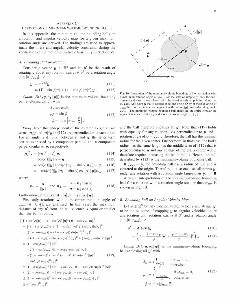
Consider a vector y ∈ R3 and let y′ be the result of

rotating y about any rotation axis n ∈ S2 by a rotation angle

ϕ ∈ [0, ϕmax], i.e.

y′ = e[ϕn]y, (111)

=(

I + sinϕ[n] + (1− cosϕ) [n]2)

y. (112)

Claim: B(δfy, ρf‖y‖) is the minimum-volume bounding

ball enclosing all y′, with

δf = cos ϕ,

ρf = sin ϕ,

ϕ = min[

ϕmax,π

2

]

.

(113)

Proof: Note that independent of the rotation axis, the two

terms [n]y and [n]2y in (112) are perpendicular to each other.

For an angle α ∈ [0, π] between n and y, the latter term

can be expressed by a component parallel and a component

perpendicular to y, respectively,

[n]2y =(

nnT − I)

y, (114)

= cos(α)‖y‖n− y, (115)

= cos(α)‖y‖(

cos(α)n‖ + sin(α)n⊥

)

− y, (116)

= − sin(α)2‖y‖n‖ + sin(α) cos(α)‖y‖n⊥, (117)

where

n‖ =y

‖y‖ , and n⊥ =n− n‖ cos(α)

‖n− n‖ cos(α)‖. (118)

Furthermore, it holds that ‖[n]y‖ = sin(α)‖y‖.

First only rotations with a maximum rotation angle of

ϕmax ∈ [0, π2 ], are analyzed. In this case, the maximum

distance of any y′ from the ball’s center is equal or smaller

than the ball’s radius,

∥∥(I + sin(ϕ)[n] + (1− cos(ϕ)) [n]2

)y − cos(ϕmax)y

∥∥2

=∥∥(1− cos(ϕmax))y + (1− cos(ϕ))[n]2y + sin(ϕ)[n]y

∥∥2

=((1− cos(ϕmax))− (1− cos(ϕ)) sin(α)2

)2 ‖y‖2

+((1− cos(ϕ)) sin(α) cos(α)

)2 ‖y‖2 +(sin(ϕ) sin(α)

)2 ‖y‖2

= (1− cos(ϕmax))2 ‖y‖2

− 2(1− cos(ϕmax))(1 − cos(ϕ)) sin(α)2‖y‖2

+ (1− cos(ϕ))2 sin(α)2(sin(α)2 + cos(α)2

)‖y‖2 (119)

+ sin2(ϕ) sin(α)2‖y‖2

= (1 − cos(ϕmax))2 ‖y‖2 + 2 cos(ϕmax)(1 − cos(ϕ)) sin(α)2 ‖y‖2

≤((1− cos(ϕmax))

2 + 2 cos(ϕmax)(1 − cos(ϕ)))‖y‖2

≤((1− cos(ϕmax))

2 + 2 cos(ϕmax)(1 − cos(ϕmax)))‖y‖2

≤ sin(ϕmax)2‖y‖2,

O

y

ϕmax

ϕmax

y1

y2

δf‖y‖

ρf‖y‖

e[ϕn]y

Fig. 10: Illustration of the minimum-volume bounding ball on a rotation witha maximum rotation angle of ϕmax. For the sake of simplicity, only the two-dimensional case is considered with the rotation axis n pointing along they3-axis. Any point y that is rotated about the origin O by at most an angle ofϕmax lies on the circular arc segment with radius ‖y‖ and subtending angle2ϕmax. The minimum-volume bounding ball enclosing the entire circular arcsegment is centered at δfy and has a radius of length ρf‖y‖.

and the ball therefore encloses all y′. Note that (119) holds

with equality for any rotation axis perpendicular to y and a

rotation angle of ϕ = ϕmax. Therefore, the ball has the minimal

radius for the given center. Furthermore, in that case, the ball’s

radius has the same length as the middle term of (112) that is

perpendicular to y and any change of the ball’s center would

therefore require increasing the ball’s radius. Hence, the ball

described by (113) is the minimum-volume bounding ball.

If ϕmax = π2 , the bounding ball has a radius of ‖y‖ and is

centered at the origin. Therefore, it also encloses all points y′

under any rotation with a rotation angle larger than π2 . �

A visual interpretation of the minimum-volume bounding

ball for a rotation with a rotation angle smaller than ϕmax is

shown in Fig. 10.

B. Bounding Ball on Angular Velocity Map

Let y ∈ R3 be any rotation vector velocity and define y′

to be the outcome of mapping y to angular velocities under

any rotation with rotation axis n ∈ S2 and a rotation angle

ϕ ∈ [0, ϕmax], i.e.

y′ = W (ϕn)y, (120)

=

(

I − 1− cosϕ

ϕ[n] +

ϕ− sinϕ

ϕ[n]2

)

y. (121)

Claim: B(δωy, ρω‖y‖) is the minimum-volume bounding

ball enclosing all y′ with

δω =

{

1, if ϕmax = 0,sin(ϕ)

ϕ, otherwise,

ρω =

{

0, if ϕmax = 0,1−cos(ϕ)

ϕ, otherwise,

ϕ = min[ϕmax, ϕ],

(122)

16

where ϕ is defined the to be the rotation angle at which the

ball radius is maximized,

ϕ := argmaxϕ>0

1− cos(ϕ)

ϕ. (123)

Proof: Equation (121) is of the same form as (112) and

therefore the proof follows the same argumentation as for the

minimum-volume bounding ball on rotations.

First, it can easily be verified that (122) is the minimum-

volume bounding ball for ϕmax = 0. Next, rotations with a

maximum rotation angle of ϕmax ∈ (0, ϕ] are considered. As

in (119), it can be shown that the maximum distance of y′ from

the ball’s center is equal or smaller than the ball’s radius, i.e.∥∥∥∥

(

I − 1− cos(ϕ)

ϕ[n] +

ϕ− sin(ϕ)

ϕ[n]2

)

y − sin(ϕmax)

ϕmax

y

∥∥∥∥

2

≤(1− cos(ϕmax)

ϕmax

)2

‖y‖2,(124)

and that the ball therefore encloses all y′. Equation (124) holds

with equality for any rotation axis perpendicular to y and a

rotation angle of ϕ = ϕmax. Following the same argumentation

as for the bounding ball on rotations, any change of the ball’s

center would require to increase the ball’s radius and hence

the ball described by (122) is the minimum-volume bounding

ball under any rotation with a maximum rotation angle of

ϕmax = ϕ.

Furthermore, again closely following the proof in (119), it

can also be shown that∥∥∥∥

(

I − 1− cos(ϕ)

ϕ[n] +

ϕ− sin(ϕ)

ϕ[n]2

)

y − sin(ϕ)

ϕy

∥∥∥∥

2

≤(1− cos(ϕ)

ϕ

)2

‖y‖2(125)

holds for any ϕ > 0, which implies that all y′ under rotations

with a rotation angle ϕ > ϕ are enclosed by the bounding ball

for a maximum angle of ϕmax = ϕ. �

ACKNOWLEDGEMENT

This work is supported by and builds upon prior contribu-

tions by numerous collaborators in the Flying Machine Arena.

A list of past and present participants of the project is available

at http://flyingmachinearena.org.

This research was supported by the Swiss National Science

Foundation (SNSF).

REFERENCES

[1] B. Crowther, A. Lanzon, M. Maya-Gonzalez, and D. Langkamp, “Kine-matic analysis and control design for a nonplanar multirotor vehicle,”Journal of Guidance, Control, and Dynamics, vol. 34, no. 4, pp. 1157–1171, 2011.

[2] E. Kaufman, K. Caldwell, D. Lee, and T. Lee, “Design and developmentof a free-floating hexrotor uav for 6-dof maneuvers,” in 2014 IEEE

Aerospace Conference, Mar. 2014, pp. 1–10.

[3] G. Jiang and R. Voyles, “A nonparallel hexrotor uav with faster responseto disturbances for precision position keeping,” in 2014 IEEE Interna-tional Symposium on Safety, Security, and Rescue Robotics, Oct. 2014,pp. 1–5.

[4] M. Ryll, D. Bicego, and A. Franchi, “Modeling and control of fast-hex:A fully-actuated by synchronized-tilting hexarotor,” in 2016 IEEE/RSJ

International Conference on Intelligent Robots and Systems (IROS), Oct.2016, pp. 1689–1694.

[5] S. Park, J. Her, J. Kim, and D. Lee, “Design, modeling and control ofomni-directional aerial robot,” in 2016 IEEE/RSJ International Confer-ence on Intelligent Robots and Systems (IROS), Oct. 2016, pp. 1570–1575.

[6] D. Brescianini and R. D’Andrea, “Design, modeling and control of anomni-directional aerial vehicle,” in 2016 IEEE International Conference

on Robotics and Automation (ICRA), May 2016, pp. 3261–3266.

[7] G. Hoffmann, S. Waslander, and C. Tomlin, “Quadrotor helicoptertrajectory tracking control,” in 2008 AIAA Guidance, Navigation andControl Conference and Exhibit, Aug. 2008, pp. 7410–7423.

[8] I. D. Cowling, O. A. Yakimenko, J. F. Whidborne, and A. K. Cooke, “Aprototype of an autonomous controller for a quadrotor UAV,” in 2007

European Control Conference (ECC). IEEE, 2007, pp. 4001–4008.

[9] Y. Bouktir, M. Haddad, and T. Chettibi, “Trajectory planning fora quadrotor helicopter,” in 2008 16th Mediterranean Conference on

Control and Automation. IEEE, 2008, pp. 1258–1263.

[10] M. Hehn and R. D’Andrea, “Real-time trajectory generation for quadro-copters,” IEEE Transactions on Robotics, vol. 31, no. 4, pp. 877–892,Aug. 2015.

[11] D. Mellinger and V. Kumar, “Minimum snap trajectory generation andcontrol for quadrotors,” in 2011 IEEE International Conference on

Robotics and Automation (ICRA), May 2011, pp. 2520–2525.

[12] C. Richter, A. Bry, and N. Roy, “Polynomial trajectory planning foraggressive quadrotor flight in dense indoor environments,” in Robotics

Research. Springer, 2016, pp. 649–666.

[13] M. W. Mueller, M. Hehn, and R. D’Andrea, “A computationally ef-ficient motion primitive for quadrocopter trajectory generation,” IEEETransactions on Robotics, vol. 31, no. 6, pp. 1294–1310, Dec. 2015.

[14] M. Hehn, R. Ritz, and R. D’Andrea, “Performance benchmarking ofquadrotor systems using time-optimal control,” Autonomous Robots,vol. 33, no. 1, pp. 69–88, 2012.

[15] M. Geisert and N. Mansard, “Trajectory generation for quadrotor basedsystems using numerical optimal control,” in 2016 IEEE International

Conference on Robotics and Automation (ICRA), May 2016, pp. 2958–2964.

[16] M. Neunert, C. de Crousaz, F. Furrer, M. Kamel, F. Farshidian,R. Siegwart, and J. Buchli, “Fast nonlinear model predictive control forunified trajectory optimization and tracking,” in 2016 IEEE International

Conference on Robotics and Automation (ICRA), May 2016, pp. 1398–1404.

[17] I. Garcia and J. P. How, “Trajectory optimization for satellite recon-figuration maneuvers with position and attitude constraints,” in 2005

American Control Conference (ACC). IEEE, 2005, pp. 889–894.

[18] H. Nguyen and Q.-C. Pham, “Time-optimal path parameterization ofrigid-body motions: Applications to spacecraft reorientation,” Journal

of Guidance, Control, and Dynamics, vol. 39, no. 7, pp. 1667–1671,2016.

[19] N. Michael, D. Mellinger, Q. Lindsey, and V. Kumar, “The grasp mul-tiple micro-uav testbed,” IEEE Robotics Automation Magazine, vol. 17,no. 3, pp. 56–65, Sep. 2010.

[20] S. Lupashin, M. Hehn, M. W. Mueller, A. P. Schoellig, M. Sherback, andR. D’Andrea, “A platform for aerial robotics research and demonstration:The flying machine arena,” Mechatronics, vol. 24, no. 1, pp. 41–54,2014.

[21] L. E. Kavraki, P. Svestka, J.-C. Latombe, and M. H. Overmars, “Prob-abilistic roadmaps for path planning in high-dimensional configurationspaces,” IEEE Transactions on Robotics and Automation, vol. 12, no. 4,pp. 566–580, 1996.

[22] S. M. LaValle and J. James J. Kuffner, “Randomized kinodynamicplanning,” The International Journal of Robotics Research, vol. 20,no. 5, pp. 378–400, 2001.

[23] C. E. Garcia, D. M. Prett, and M. Morari, “Model predictive control:theory and practicea survey,” Automatica, vol. 25, no. 3, pp. 335–348,1989.

[24] M. D. Shuster, “A survey of attitude representations,” Navigation, vol. 8,no. 9, pp. 439–517, 1993.

[25] R. Mahony, V. Kumar, and P. Corke, “Multirotor aerial vehicles: Mod-eling, estimation, and control of quadrotor,” IEEE Robotics Automation

Magazine, vol. 19, no. 3, pp. 20–32, Sept 2012.

[26] D. P. Bertsekas, Dynamic Programming and Optimal Control. AthenaScientific, 2005.

[27] S. Tanygin, “Attitude interpolation,” in AAS/AIAA Spaceflight Mechanics

Meeting, Feb. 2003.

[28] P. Borwein and T. Erdelyi, Polynomials and polynomial inequalities.Springer Science & Business Media, 2012, vol. 161.

17

[29] M. A. Patterson and A. V. Rao, “GPOPS-II: A matlab software forsolving multiple-phase optimal control problems using hp-adaptive gaus-sian quadrature collocation methods and sparse nonlinear programming,”ACM Transactions on Mathematical Software (TOMS), vol. 41, no. 1,pp. 1–37, Oct. 2014.

[30] W. C. Durham, “Attainable moments for the constrained control allo-cation problem,” Journal of Guidance, Control, and Dynamics, vol. 17,no. 6, pp. 1371–1373, 1994.

[31] A. E. Bryson and Y.-C. Ho, Applied Optimal Control: Optimization,Estimation and Control. Ginn and Company, 1969.

Dario Brescianini received the B.Sc. and theM.Sc. degrees in mechanical engineering from ETHZurich, Zurich, Switzerland, in 2010 and 2013, re-spectively. He received the Outstanding D-MAVTBachelor Award and was awarded the Willi-Studerprize for the best Master’s degree in Robotics, Sys-tems, and Control.

He is currently a PhD student at the Institute forDynamic Systems and Control, ETH Zurich. Hismain research interests include aerial vehicle design,the control and trajectory generation of multirotor

vehicles, and learning algorithms.

Raffaello D’Andrea received the B.Sc. degree inEngineering Science from the University of Toronto,Toronto, ON, Canada, in 1991, and the M.S. andPh.D. degrees in Electrical Engineering from theCalifornia Institute of Technology, Pasadena, CA,USA, in 1992 and 1997, respectively.

He was an Assistant and then an Associate Pro-fessor with Cornell University, Ithaca, NY, USA,from 1997 to 2007. While on leave from CornellUniversity, from 2003 to 2007, he cofounded KivaSystems, North Reading, MA, USA, where he led

the systems architecture, robot design, robot navigation and coordination, andcontrol algorithms efforts. He is currently a Professor of Dynamic Systemsand Control at ETH Zurich, Zurich, Switzerland, and chairman of the boardat Verity Studios AG, Zurich, Switzerland.