computer aided analysis of mr brain images - …etd.dtu.dk/thesis/57990/imm766.pdf · computer...
TRANSCRIPT

Computer AidedAnalysis of
MR Brain Images
Stefan Wolff
Kgs. LYNGBY 2001EKSAMENSPROJEKT
NR. 08/2001
IMM

Trykt af IMM, DTU

Preface
This thesis has been prepared at the numerical analysis section of Informaticsand Mathematical Modelling (IMM) at the Technical University of Denmark(DTU) in partial fulfillment of the requirement for the degree of Master of Sci-ence in Engineering.
During this work I have had the privilege of cooperating with a group oftruly delightful people. First of all I would like to thank my advisor, Per SkafteHansen, for his encouragement, flexibility, and commitment. I would also liketo thank Lars G. Hanson and Torben Lund (Danish Research Center for Mag-netic Resonance) for always being ready to share their knowledge of the scienceof magnetic resonance and state-of-the-art MRI techniques, as well as for theircontagious enthusiasm. I am also indebted to Margrethe Herning and Anne-Mette Leffers (DRCMR) for suggestions for improvements and for lifting a cor-ner of the veil obscuring the esoteric field of Yedi radiology. Next, I would liketo thank the Oticon Foundation for supporting this work. I would also like tothank the faculty, staff and students of the numerical analysis section of IMMfor providing a stimulating and relaxed environment.
Finally, I would like to thank my friends and the members of my family foreach providing someone to miss.
Kgs. Lyngby, Denmark, August 31st, 2001Stefan Wolff

ii

Summary
Cortical dysplasia, the malformation of the cerebral cortex (the layer of graymatter forming the surface of the brain), can take on a number of forms, suchas:
� A thickening of the cortex� A diffuse organization, with white and gray matter apparently mixing� Brain geometry deformation� Heterotopia, the misplacement of gray matter inside white
The object of the work reported here is to provide a clinical expert (a radiol-ogist) with an algorithmic tool that will assist in the detection of the first two ofthese. The algorithm analyzes 3D data sets, obtained as luminance level valuesrepresenting the output from MR scans of the human brain. The data is orga-nized as a voxel image, with a geometry representing a straightforward dis-cretization of that of the brain under study. The only information available asto the category of a given voxel (gray matter, white matter, cerebro-spinal fluid,vascular tissue or background) is that of the luminance level. An automatedsegregation will suppress precisely the information sought by the present al-gorithm, while (time-consuming) human intervention would be tantamount toa solution of the problem addressed. The algorithms are developed with thislimitation observed throughout.
Keywords
Magnetic Resonance, Cortical Dysplasia, Gradient Correlation Algorithm, VoxelImages, Visualization.

iv
Dansk resume
Cortical dysplasi, fejludvikling af hjernebarken (et lag af gra substans der udgørhjernens overflade) kan give sig udtryk pa adskillige mader, sasom:
� Fortykkelse af hjernebarken� Diffus overgang fra gra til hvid substans� Deformation af hjernen� Heterotopi: gra substans fejlplaceret inde i hvid substans
Hensigten med nærværende arbejde er at udruste en klinisk ekspert (en ra-diolog) med et algoritmisk værktøj der kan hjælpe med at detektere forekom-ster af de første to af de ovennævnte fænomener. Algoritmen analyserer 3D-datasæt bestaende af luminansværdier fremkommet af MR-skanninger af enmenneskehjerne. Data er organiseret som et voxel-billede, hvis geometri hidrørerfra en direkte diskretisering af den undersøgte hjerne. Den eneste til radighedstaende information, der kan give et fingerpeg om vævstypen (gra substans,hvid substans, cerebro-spinal væske, karvæv eller baggrund) er luminansvær-dien. En automatisk inddeling vil undertrykke netop den information, dersøges af den her præsenterede algoritme, og (tidskrævende) menneskelig ind-blanden ville svare til en løsning pa problemet. Algoritmerne er udviklet meddenne begrænsning.

vi
Contents
1 Introduction 1
2 Introductory Theory 52.1 Magnetic Resonance Imaging Basics . . . . . . . . . . . . . . . . 5
2.1.1 Scanner output . . . . . . . . . . . . . . . . . . . . . . . . 62.1.2 Multi-Planar Reformatting . . . . . . . . . . . . . . . . . 7
2.2 On Rendering, Image Processing, and Image Analysis . . . . . . 72.2.1 Texture Mapping . . . . . . . . . . . . . . . . . . . . . . . 72.2.2 Coordinate Systems . . . . . . . . . . . . . . . . . . . . . 82.2.3 On Discrete Regular Grids . . . . . . . . . . . . . . . . . . 102.2.4 Gradient Fields . . . . . . . . . . . . . . . . . . . . . . . . 102.2.5 Resampling . . . . . . . . . . . . . . . . . . . . . . . . . . 11
2.3 On the Human Brain . . . . . . . . . . . . . . . . . . . . . . . . . 112.3.1 Cortical Dysplasia . . . . . . . . . . . . . . . . . . . . . . 12
2.4 Detection of Dysplastic Lesions . . . . . . . . . . . . . . . . . . . 132.5 Consequences . . . . . . . . . . . . . . . . . . . . . . . . . . . . . 132.6 Important Names and Concepts . . . . . . . . . . . . . . . . . . . 14
3 Prior Work 173.1 Curvilinear Reformatting . . . . . . . . . . . . . . . . . . . . . . 173.2 Shear-Warp Rendering . . . . . . . . . . . . . . . . . . . . . . . . 173.3 Other Render Methods . . . . . . . . . . . . . . . . . . . . . . . . 193.4 Voxel-Based Morphometry . . . . . . . . . . . . . . . . . . . . . . 19
4 Purpose 234.1 Detection . . . . . . . . . . . . . . . . . . . . . . . . . . . . . . . . 23
4.1.1 Assumptions . . . . . . . . . . . . . . . . . . . . . . . . . 244.1.2 Constraints . . . . . . . . . . . . . . . . . . . . . . . . . . 24
4.2 Visualization . . . . . . . . . . . . . . . . . . . . . . . . . . . . . . 254.3 An Overview of this Thesis . . . . . . . . . . . . . . . . . . . . . 25
5 Two-Dimensional Display 295.1 Rendering the intermediate image . . . . . . . . . . . . . . . . . 29
5.1.1 Intensity Determination . . . . . . . . . . . . . . . . . . . 305.1.2 Intensity Mapping . . . . . . . . . . . . . . . . . . . . . . 305.1.3 A Slight Improvement . . . . . . . . . . . . . . . . . . . . 31
5.2 Applying the texture map . . . . . . . . . . . . . . . . . . . . . . 325.3 Possible improvements . . . . . . . . . . . . . . . . . . . . . . . . 33
viii CONTENTS
6 Three-Dimensional Rendering 356.1 Shear-Warp Rendering . . . . . . . . . . . . . . . . . . . . . . . . 35
6.1.1 Spatial Coherency . . . . . . . . . . . . . . . . . . . . . . 376.1.2 The Shear-Warp Factorization . . . . . . . . . . . . . . . . 37
6.2 Modifications for Interactive Display . . . . . . . . . . . . . . . . 386.3 Combining Voxels and Polygons . . . . . . . . . . . . . . . . . . 38
6.3.1 Generating Depth Information . . . . . . . . . . . . . . . 386.3.2 Limited buffer resolution . . . . . . . . . . . . . . . . . . 416.3.3 Contour Drawing . . . . . . . . . . . . . . . . . . . . . . . 426.3.4 Phong Illumintation . . . . . . . . . . . . . . . . . . . . . 456.3.5 Possible Improvements . . . . . . . . . . . . . . . . . . . 476.3.6 Alternatives . . . . . . . . . . . . . . . . . . . . . . . . . . 47
6.4 Disadvantages of Shear-Warp Rendering . . . . . . . . . . . . . 47
7 Curvilinear Reformatting 517.1 Brain Extraction Tool . . . . . . . . . . . . . . . . . . . . . . . . . 517.2 Surface Extraction . . . . . . . . . . . . . . . . . . . . . . . . . . . 517.3 Other Metrics . . . . . . . . . . . . . . . . . . . . . . . . . . . . . 52
8 Dysplastic Lesion Detection Aid 578.1 Intensity Thresholding . . . . . . . . . . . . . . . . . . . . . . . . 578.2 Gradient Correlation . . . . . . . . . . . . . . . . . . . . . . . . . 588.3 Cluster Sizes . . . . . . . . . . . . . . . . . . . . . . . . . . . . . . 598.4 Alternatives . . . . . . . . . . . . . . . . . . . . . . . . . . . . . . 628.5 Discussion . . . . . . . . . . . . . . . . . . . . . . . . . . . . . . . 62
8.5.1 Non-Isotropic Voxels . . . . . . . . . . . . . . . . . . . . . 638.5.2 Blur Versus Noise . . . . . . . . . . . . . . . . . . . . . . . 63
9 Prototype Implementation 659.1 General . . . . . . . . . . . . . . . . . . . . . . . . . . . . . . . . . 659.2 User Interaction . . . . . . . . . . . . . . . . . . . . . . . . . . . . 65
9.2.1 Selective Updating . . . . . . . . . . . . . . . . . . . . . . 669.2.2 Preprocessing . . . . . . . . . . . . . . . . . . . . . . . . . 67
9.3 Histogram Display . . . . . . . . . . . . . . . . . . . . . . . . . . 689.4 Cortical Detection . . . . . . . . . . . . . . . . . . . . . . . . . . . 689.5 Data . . . . . . . . . . . . . . . . . . . . . . . . . . . . . . . . . . . 699.6 Performance and Requirements . . . . . . . . . . . . . . . . . . . 69
10 Results 7310.1 Detection of Dysplastic Lesions . . . . . . . . . . . . . . . . . . . 7310.2 Effects of Intensity Nonuniformity . . . . . . . . . . . . . . . . . 74
11 Summary 7911.1 Main Contributions . . . . . . . . . . . . . . . . . . . . . . . . . . 7911.2 Possible Improvements . . . . . . . . . . . . . . . . . . . . . . . . 7911.3 Benefits . . . . . . . . . . . . . . . . . . . . . . . . . . . . . . . . . 8011.4 Future Work . . . . . . . . . . . . . . . . . . . . . . . . . . . . . . 8011.5 Conclusion . . . . . . . . . . . . . . . . . . . . . . . . . . . . . . . 81
A Selected Images 83

CONTENTS ix
B Resources on the Internet 91
Bibliography 93

x CONTENTS
List of Figures
2.1 Multi-planar reformatting . . . . . . . . . . . . . . . . . . . . . . 72.2 Gray matter illusion I . . . . . . . . . . . . . . . . . . . . . . . . . 82.3 Gray matter illusion II . . . . . . . . . . . . . . . . . . . . . . . . 92.4 3D gradient filter mask . . . . . . . . . . . . . . . . . . . . . . . . 112.5 Linear interpolation . . . . . . . . . . . . . . . . . . . . . . . . . . 12
3.1 The idea behind curvilinear reformatting . . . . . . . . . . . . . 183.2 Ray casting using the shear-warp factorization. . . . . . . . . . . 18
4.1 Prototype graphical user interface layout showing a cube . . . . 25
5.1 Different resampling techniques . . . . . . . . . . . . . . . . . . 305.2 Intensity mapping . . . . . . . . . . . . . . . . . . . . . . . . . . . 315.3 Pixel skipping . . . . . . . . . . . . . . . . . . . . . . . . . . . . . 32
6.1 Image and corresponding depth image . . . . . . . . . . . . . . . 396.2 Generating depth information . . . . . . . . . . . . . . . . . . . . 406.3 Different kinds of slice indication . . . . . . . . . . . . . . . . . . 436.4 The contour artifact . . . . . . . . . . . . . . . . . . . . . . . . . . 446.5 Phong illumination vectors . . . . . . . . . . . . . . . . . . . . . 456.6 Holes in shear-warp images . . . . . . . . . . . . . . . . . . . . . 48
7.1 Curvilinear reformatting . . . . . . . . . . . . . . . . . . . . . . . 53
8.1 Part of a typical intensity histogram. . . . . . . . . . . . . . . . . 588.2 Two-dimensional examples of the measure of cluster size. . . . . 608.3 Detection of dysplastic lesions, step by step . . . . . . . . . . . . 61
9.1 Screenshot of the graphics display . . . . . . . . . . . . . . . . . 669.2 Screenshot with detected dysplasia . . . . . . . . . . . . . . . . . 679.3 Emphasizing cortical structure . . . . . . . . . . . . . . . . . . . 68
10.1 Detected focal dysplasias . . . . . . . . . . . . . . . . . . . . . . . 7410.2 Effect of parameter variation . . . . . . . . . . . . . . . . . . . . . 7510.3 False detections due to intensity nonuniformity . . . . . . . . . . 75
A.1 Screenshot with detected dysplasia . . . . . . . . . . . . . . . . . 84A.2 Screenshot with detected dysplasia . . . . . . . . . . . . . . . . . 85A.3 Detected focal dysplasias . . . . . . . . . . . . . . . . . . . . . . . 86A.4 Effect of parameter variation . . . . . . . . . . . . . . . . . . . . . 87

xii LIST OF FIGURES
A.5 Effect of parameter variation . . . . . . . . . . . . . . . . . . . . . 88A.6 False detections due to intensity nonuniformity . . . . . . . . . . 89

LIST OF FIGURES xiii


Chapter 1
Introduction
The advent of the possibility of visualizing the interior of the human bodywithout surgical intervention has had a significant impact on the world ofmedical science ever since the discovery of x-rays. One fairly recent imagingmodality, known as magnetic resonance imaging (MRI), offers detailed imagesof the human anatomy with high soft tissue contrast. Owing to the multitudeof imaging parameters involved, and the fact that, unlike many other modal-ities, MRI is not confined to transverse cross-sections, it constitutes a versa-tile way of performing non-invasive in vivo evaluation of tissue anatomy, flow,metabolism, etc.
As MR examinations become routine in many hospitals, the problem arisesof combing through the vast amount of generated data. Conventional visu-alization media such as film sheets and computer screens are inherently two-dimensional, rendering them incapable of displaying true three-dimensionaldata sets. Attempts to overcome this limitation, e.g. by imposing transparency,are likely to fail in the general case because of the reduced dimensionality in-volved. Clinical examiners (radiologists) have to make do with two-dimensionaldata, in the form of planar or curvilinear slices.
The purpose of the work presented here is to provide a clinical expert (aradiologist) with a way of overcoming the reduced dimensionality inherent inconventional media by the development of a tool to assist in searching throughlarge 3D magnetic resonance (MR) images. This tool has been specifically ap-plied to the visualization and detection of development disorders, known asfocal cortical dysplasia, in the layer of gray matter forming the surface of thebrain (the cerebral cortex). Disorders of this kind are associated with epilepsy.Although subtle dysplastic lesions may not have any direct effect on the intel-lect, the effects of medication and frequent epileptic seizures may lead to cog-nitive impairment. Owing to drug resistance or medically refractory epilepsy,surgery may provide the only solution. Subtle lesions often show good prog-noses for surgical intervention, but may be hard to detect owing to their sub-tlety as well as the level of noise in the MR image. Even for an expert radiol-ogist, subtle lesions may take days to detect, wherefore any reduction in thetime spent searching would be beneficial.
This thesis describes an algorithm originating from 3D image analysis for au-tomatic detection of key symptoms of focal dysplasia. The algorithm is embed-

2 Introduction
ded in a real-time graphics system to facilitate the reading and interpretationof results. A description of key features of this graphics system as well as ashort introduction to relevant subjects are also included in the thesis.
The reader is assumed to be familiar with basic computer graphics and im-age analysis. Prior knowledge of magnetic resonance and MRI is not a prereq-uisite.
A related paper was submitted to the 10th international conference on DiscreteGeometry for Computer Imagery in Bordeaux, France.
This work was supported in part by a grant from the Oticon Foundation.

Introduction 3


Chapter 2
Introductory Theory
This chapter attempts to give the reader sufficient insight into image process-ing, magnetic resonance imaging (MRI), and the human brain so as to makeaccessible the subsequent chapters of this thesis. It is by no means intended asa comprehensive treatment of the subjects.
The next chapter similarly covers the prior work on which the method pre-sented here is based.
The contributions comprising the kernel of this thesis are presented fromchapter 4 and onwards.
2.1 Magnetic Resonance Imaging Basics
Ensembles of atomic nuclei possessing an odd number of neutrons or protonsexhibit behaviour comparable to that of a compass needle, that is to say theseensembles, when placed in a magnetic field, tend to align in the direction of thisfield. This alignment does not happen instantly, but takes some time depend-ing on the surroundings of each nuclei as well as the strength of the appliedmagnetic field. This gradual alignment is called relaxation. During this relax-ation, the ensembles precess in the plane perpendicular to the applied field ata frequency called the Larmor frequency, which is defined by
f =
2�B ; (2.1)
where f is the resonance frequency, B is the field strength, and , called the gy-romagnetic ratio, is a number depending on the type of nuclei. This transversalcomponent of the magnetization is detectable, since the magnetic change mayinduce a current in an appropriately positioned reveicer coil. The temporalsignal represented by this current is called the free induction decay (FID).
The relaxation is approximately exponential, but longitudinal and transver-sal relaxation need not happen at the same rate. This means the compass needleanalogy breaks down, since the length of the needle, corresponding to magne-tization strength, may change during relaxation. The longitudinal relaxationtime constant is denoted by T1 and its transversal counterpart is denoted byT2. Different tissue types have (slightly) different time constants – in actuality,

6 Introductory Theory
these time constant differences are often what is being depicted. MR imagesemphasizing differences in T1 are known as T1-weighted images, whereas thosedifferentiating tissue types by their T2 time constants are known as T2-weightedimages.
When the ensembles have been subject to the above static magnetic field(known as the main field) for some time, a state of equilibrium is reached andthe ensembles no longer exhibit any measurable precession. However, by ap-plying a transverse magnetic field pulsating at the Larmor frequency, it is pos-sible to force the ensembles out of this equilibrium. This process is known asmagnetic resonance, and the applied field is known as the excitation, or radiofre-quency (RF) field, as the Larmor frequencies are usually within the RF range.By applying a third kind of magnetic field, a field that varies with position,it is possible to encode positional information into the received signal (FID),thus enabling the transformation from FID to MR image. This third kind ofmagnetic field is known as a gradient field.
However, applying such an inhomogeneous magnetic field leads to phasedispersion, or destructive (neutralizing) interference, which causes the FID todeteriorate. One way of reducing this problem is by using gradient echoes. As-sume that all ensembles (“compass needles”) are in-phase at time t = 0. Fur-ther assume that a gradient field is applied at time t = 0 in addition to a mainfield. At the time t = � , the gradient field has caused some phase dispersion.Assume that the gradient field is somehow reversed at time t = � . This meansthat the ensembles that lost phase when compared to ensembles unaffected bythe gradient field now gain phase, and vice versa. At time t = 2� , the ensem-bles have rephased, causing a so-called gradient echo. By sampling the FID closeto this echo, the signal-weakening dephasing caused by the gradient fields willbe reduced.
For a thorough treatment of the subject of magnetic resonance imaging, re-fer to [Nish94]. For a treatment in Danish, including a brief description of theMR phenomenon based on quantum theory, see [Wolf01].
2.1.1 Scanner output
The usual MRI sequence used for identifying cortical dysplasia is called MP-RAGE (see [Bran92]), which stands for Magnetization Prepared Rapid GradientEcho. This is the gradient echo technique described above, preceded by aninitial 180Æ excitation performed to further enhance the T1 dependency of theimage. This is an MR sequence producing a three-dimensional T1-weightedimage with (typically) near-isotropic voxels. In these images, the main compo-nents (see section 2.3) of the brain are[Edel96]:
White matter: BrightGray matter: Dark
Cerebrospinal fluid: Very dark
This imaging sequence gives good brain tissue contrast while at the sametime offering bearable scan times (� 15 minutes).
2.2 On Rendering, Image Processing, and Image Analysis 7
2.1.2 Multi-Planar Reformatting
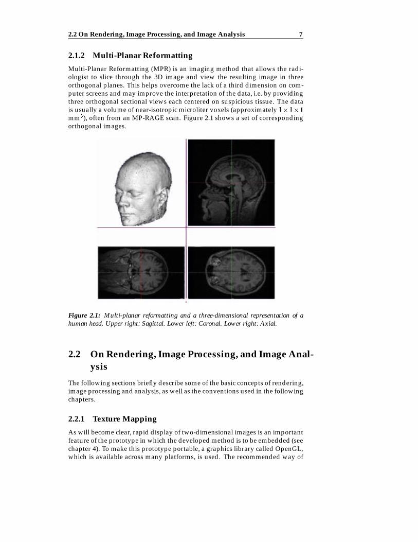
Multi-Planar Reformatting (MPR) is an imaging method that allows the radi-ologist to slice through the 3D image and view the resulting image in threeorthogonal planes. This helps overcome the lack of a third dimension on com-puter screens and may improve the interpretation of the data, i.e. by providingthree orthogonal sectional views each centered on suspicious tissue. The datais usually a volume of near-isotropic microliter voxels (approximately 1�1�1mm3), often from an MP-RAGE scan. Figure 2.1 shows a set of correspondingorthogonal images.
Figure 2.1: Multi-planar reformatting and a three-dimensional representation of ahuman head. Upper right: Sagittal. Lower left: Coronal. Lower right: Axial.
2.2 On Rendering, Image Processing, and Image Anal-ysis
The following sections briefly describe some of the basic concepts of rendering,image processing and analysis, as well as the conventions used in the followingchapters.
2.2.1 Texture Mapping
As will become clear, rapid display of two-dimensional images is an importantfeature of the prototype in which the developed method is to be embedded (seechapter 4). To make this prototype portable, a graphics library called OpenGL,which is available across many platforms, is used. The recommended way of
8 Introductory Theory
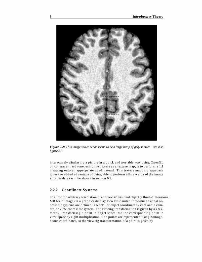
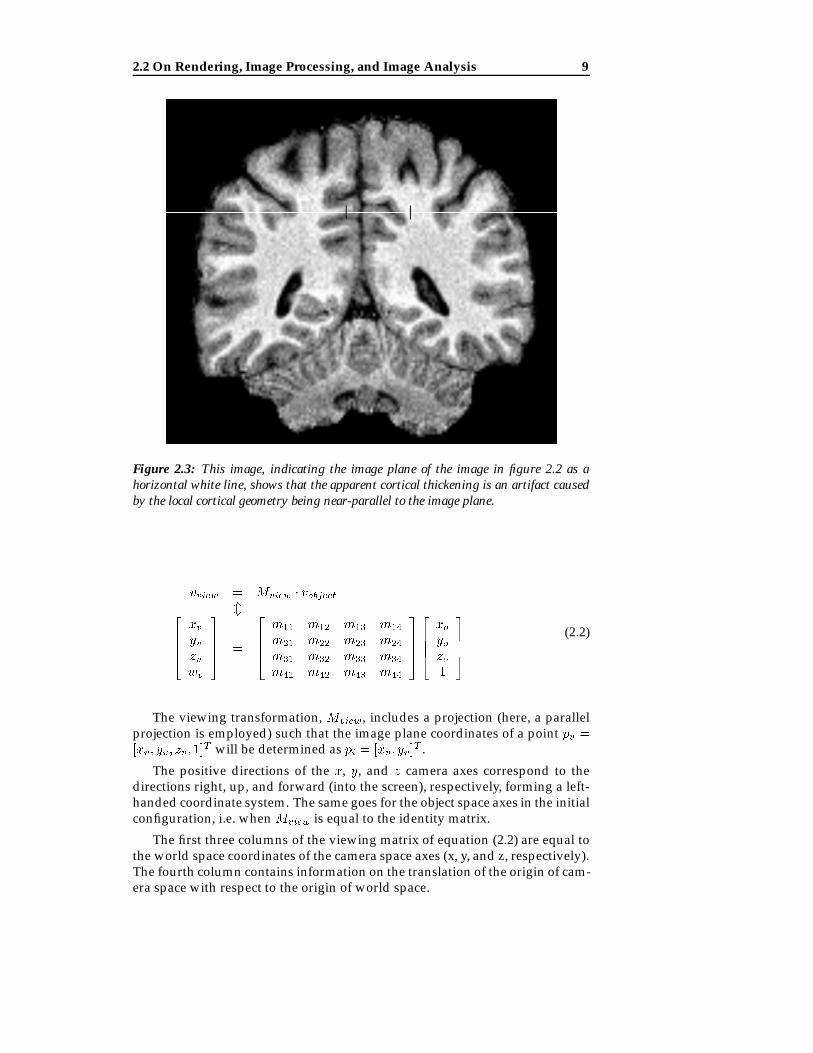
Figure 2.2: This image shows what seems to be a large lump of gray matter – see alsofigure 2.3.
interactively displaying a picture in a quick and portable way using OpenGLon consumer hardware, using the picture as a texture map, is to perform a 1:1mapping onto an appropriate quadrilateral. This texture mapping approachgives the added advantage of being able to perform affine warps of the imageeffortlessly, as will be shown in section 6.2.
2.2.2 Coordinate Systems
To allow for arbitrary orientation of a three-dimensional object (a three-dimensionalMR brain image) in a graphics display, two left-handed three-dimensional co-ordinate systems are defined: a world, or object coordinate system and a cam-era, or view coordinate system. The viewing transformation is given by a 4�4-matrix, transforming a point in object space into the corresponding point inview space by right multiplication. The points are represented using homoge-neous coordinates, so the viewing transformation of a point is given by
2.2 On Rendering, Image Processing, and Image Analysis 9
Figure 2.3: This image, indicating the image plane of the image in figure 2.2 as ahorizontal white line, shows that the apparent cortical thickening is an artifact causedby the local cortical geometry being near-parallel to the image plane.
vview = Mview � vobjectm2
664xvyvzvwv
3775 =
2664
m11 m12 m13 m14
m21 m22 m23 m24
m31 m32 m33 m34
m41 m42 m43 m44
37752664
xoyozo1
3775
(2.2)
The viewing transformation, Mview, includes a projection (here, a parallelprojection is employed) such that the image plane coordinates of a point pv =[xv ; yv; zv; 1]
T will be determined as pi = [xv ; yv]T .
The positive directions of the x, y, and z camera axes correspond to thedirections right, up, and forward (into the screen), respectively, forming a left-handed coordinate system. The same goes for the object space axes in the initialconfiguration, i.e. when Mview is equal to the identity matrix.
The first three columns of the viewing matrix of equation (2.2) are equal tothe world space coordinates of the camera space axes (x, y, and z, respectively).The fourth column contains information on the translation of the origin of cam-era space with respect to the origin of world space.
10 Introductory Theory
2.2.3 On Discrete Regular Grids
The data obtained from an MR scanner sequence suitable for MPR is normally aset of near-isotropic voxels on a regular grid. A number of metrics lend them-selves to distance determination in such a grid. In this thesis, however, theemployed metric is the Euclidean distance between voxel centers. Other met-rics and their impacts on the developed method will be discussed in section7.3. The work presented here will assume isotropic voxels – the case of non-isotropic voxels will be discussed in section 8.5.1.
2.2.4 Gradient Fields
To an intensity field, such as a three-dimensional volume of intensities outputby an MR scanner, can be associated a so-called gradient field1, which is a vectorfield displaying the rate of change of the intensity field, each vector showingthe direction of maximum change.
To represent the digital approximation of the gradient, the symbolr (nabla),conventionally used to denote the gradient of a continuous field, is used.
As a one-dimensional example, determining the gradient along a line ofpixels with no attention paid to scaling, one could use the following expressionto approximate the gradient of the n’th pixel rn, using the pixel intensities in:
rn = in+1 � in�1 (2.3)
Note, that the n’th element of the vector of intensities [i1; i2; i3; : : :] con-volved with the vector [1; 0;�1] leads to the same result.
In two dimensions, the gradient is a vector of two elements. The first ele-ment, representing the horizontal component of the gradient, may be derivedin the exact same way as the one-dimensional case, i.e. by convolving eachhorizontal scanline. The vertical component can be derived in a similar fash-ion, namely by convolving each vertical scanline by [1; 0;�1]T . Since this isonly an approximation of the gradient, other filter masks may provide a betterestimate. An alternative set of filter masks for 2D images are:
Mhoriz =
24 �1 0 1�2 0 2�1 0 1
35 Mvert =
24 �1 �2 �1
0 0 01 2 1
35 (2.4)
This set of masks estimates the gradient components using a larger neigh-bourhood but puts emphasis on nearer pixels. Note, that the masks have beenrotated by 180 degrees when compared to the vectors above. This is due tothe reflection between the filter mask and the point spread function: if h(k; l)is the point spread function, the filter mask elements (called filter weights) areusually given as h(�k;�l).
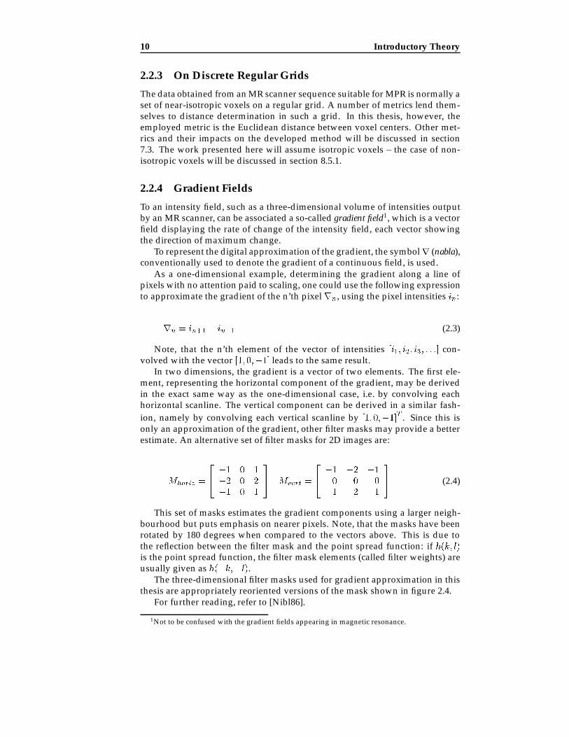
The three-dimensional filter masks used for gradient approximation in thisthesis are appropriately reoriented versions of the mask shown in figure 2.4.
For further reading, refer to [Nibl86].
1Not to be confused with the gradient fields appearing in magnetic resonance.

2.3 On the Human Brain 11
−1 −1
−1
−1−1
−2−1
−1
0
00
0
1
11
−10
0
0
0
0
1 1
11
2
1
Figure 2.4: The filter mask used for three-dimensional gradient approximation.
2.2.5 Resampling
The program offers a choice between two ways of determining the voxel inten-sity at a given position: Nearest-neighbour filtering or trilinear interpolationfiltering. The following example illustrates the problem and a few possiblesolutions.
Example 2.1: One-dimensional resampling. Assume that the values of a func-tion f(x) are sampled at integer values of x. What would be a reasonable value for,say, f(1:4) ? Using the nearest-neighbour resampling filter, the answer would be~fnn(1:4) = f(1), the value of the nearest neighbour. Using a linear resampling filter,however, the answer would be a linearly weighted average of the nearest values, i.e. apoint corresponding to x = 1:4 on the straight line between (1; f(1)) and (2; f(2)):
~flin(1:4) = (2� 1:4)f(1) + (1:4� 1)f(2) (2.5)
Refer to figure 2.5.
The nearest-neighbour resampling filter is cheaper in terms of computingtime, whereas the linear interpolation filter is considerably less “blocky”, sincethe output of the filtered function ~flin(x) is continuous.
Both the nearest-neighbour resampling filter and the linear interpolationresampling filter may be extended to higher dimensions. The latter is knownas bilinear interpolation in two dimensions (section 6.1) and trilinear interpo-lation (section 5.1.1) in three dimensions.
Non-linear resampling is another possibility, with sinc interpolation, as wellas quadratic and cubic interpolation resampling being the most popular choices.A more thorough introduction to resampling may be found in [Nibl86].
2.3 On the Human Brain
The human brain consists roughly of two kinds of tissue arranged in threelayers. In the depth close to the midline, a core of gray matter called the basal

12 Introductory Theory
x
f(x)
1
1
2
f(1.4)~
Figure 2.5: Linear interpolation between integer sample points of the function f . Referto example 2.1.
ganglia is found. The basal stuctures are surrounded by a relatively thick layerof white matter, and this is covered by an approximately 3 mm thick cortex.During the development of the cerebral cortex, which mainly takes place fromthe seventh week after conception to birth, a number of things may go wrong.One of the possible malformations is called cortical dysplasia, to which someof the associated MR imaging findings can be seen in table 2.1.
1. Cortical thickening.2. Blurred gray/white matter junction, i.e. blurred transi-
tion between gray matter and white matter.3. Brain deformation.4. Heterotopia (gray matter misplaced inside white matter).
Table 2.1: Typical MR imaging findings in dysplastic brains.
2.3.1 Cortical Dysplasia
Cortical dysplasia associated with seizure disorders are often divided into threecategories[Edel96]:
� Focal lesions, in which the amount of abnormal tissue is relatively smalland localized.
� Unilateral disorders, roughly affecting one entire cerebral hemisphere.� Generalized, or bilateral, disorders, affecting the entire brain.
The extent of the abnormal tissue in the unilateral and generalized casesmake them susceptible to easy detection by visual inspection of MR images,whereas the focal lesions may be subtle, and thus more difficult to detect.The central point in this thesis is the development of a set of tools to aid atrained neuroradiologist in locating subtle focal dysplastic lesions of Taylor
2.4 Detection of Dysplastic Lesions 13
type[Tayl71]. This type of disorder is characterized by localized cortical thick-ening and poor gray/white matter differentiation, item 1 and 2 of table 2.1,and is believed to be among the most epileptogenic lesions associated withepilepsy.
The localized cortical thickening makes the cortex of the affected regionlook like a carpet with a rock underneath. The size of the rock obviously has agreat impact on the detectability of the disorder. Mild cortical disorganizationmay be undetectable by MRI, since the affected region may be smaller than theresolution of the MR image. Section 2.4 describes the currently used techniquesfor detecting subtle cortical dysplasias of Taylor.
2.4 Detection of Dysplastic Lesions
Cortical development disorders of any of the above categories may be detectedusing conventional MPR techniques. However, in recent years, work has beendone to aid in the detection of the subtler focal lesions. Various forms of curvi-linear reformatting (CR), such as the one described in chapter 7 of this thesis,as well as methods such as voxel-based morphometry, described in the section3.4, have been proposed.
2.5 Consequences
The possibility of detection of a focal cortical dysplasia in a patient with epilepsymay take the patient from the category of life-long medication and even drugresistance to the category of possible surgical candidates. If other neurophysio-logical investigations (e.g. electro-encephalography, EEG) points to exactly thesame region and to no other regions, the prognosis for surgical intervention isvery good.

14 Introductory Theory
2.6 Important Names and Concepts
Axial Slice orientation. Bottom view. See figure 2.1.Basal ganglia A structure of gray matter forming the core of
the brain.Coronal Slice orientation. Rear view. See figure 2.1.Cerebral cortex The exterior substance of the brain. Consists of
gray matter.Cerebro-spinalfluid, CSF
A serous fluid secreted by the membranes cov-ering the brain and spinal cord. The brain“floats” in CSF.
Dysplasia Abnormal development (of organs or cells)or an abnormal structure resulting from suchgrowth.
Electro-encephalogram,EEG
A graphical record of electrical activity of thebrain
Frontal lobe The part of the cerebral cortex in either hemi-sphere of the brain lying directly behind theforehead.
Gray matter Grayish nervous tissue forming the cerebralcortex and the basal ganglia.
Gyrus, pl. gyri The convoluted ridges between the sulci.Sagittal Slice orientation. Side view. See figure 2.1.Sulcus, pl. sulci The fissures and grooves in the cerebral cortex.Temporal lobe The part of the cerebral cortex in either hemi-
sphere of the brain lying inside the temples ofthe head.
White matter Whitish nervous tissue forming a rather thicklayer on the basal ganglia.

2.6 Important Names and Concepts 15

Chapter 3
Prior Work
3.1 Curvilinear Reformatting
As a means of overcoming the lack of a third dimension inherent in computerscreens and regular MR images, it is possible to perform a virtual incision inthe MR image that allows for inspection along a given cutting surface. Thesesurfaces are most often planar (like those of MPR, see section 2.1.2), but mayalso be curvilinear, although typically limited in shape to an extrusion of amanually drawn planar curve. The extraction of curvilinear surfaces is calledcurvilinear reformatting.
Bastos et al. [Bast99] presented a new way of extracting curvilinear slices.This method allows the radiologist to examine the three-dimensional brain im-age using a series of thin slices curved along the hemispheric convexities of thebrain, much like the layers of an onion. As opposed to the planar slices offeredby conventional MPR, this may significantly reduce the impression of corticalthickening caused by obliquity of the plane of section in relation to the gyri.Figure 3.1 shows how curvilinear reformatting obtains a parallel incidence ofthe slice in relation to the gyral cortex. This reduces the artifactual corticalthickness shown in figures 2.2 and 2.3.
The method of Bastos et al. requires a neuroradiologist to manually delin-eate the brain surface. Subsequently, the software generates a set of 3D polyg-onal models including the corresponding texture maps. Following this, theactual examination takes place, during which the radiologist can display andmanipulate the previously generated curvilinear1 data, as well as planar slicesgenerated on-the-fly2.
3.2 Shear-Warp Rendering
The title of this section is shorthand for volumetric rendering using a shear-warp factorization of the viewing transformation.
This factorization can be written
1Since the generated data consists of polygonal models, it is in actuality not curvilinear.2This information was acquired through personal correspondence with Mr. Roch Comeau.

18 Prior Work
Figure 3.1: Coronal diagram showing cortex (gray) and the plane of a curved slice(black bold). Notice how the slice intersects the cortex at near-right angles.
c
b
a
Viewing rays
Slices
Image plane
a
b
c
Image planeIntermediate image plane
Warp
Shear
Figure 3.2: Ray casting using the shear-warp factorization.
Mview = Mwarp �Mshear (3.1)
The idea behind this technique is to divide the rendering process in a man-ner similar to the factorization:
1. Perform a 3D shear parallel to the data slices such that the viewing raysbecome parallel to each other and perpendicular to the slices (see figure3.2).
2. Project the sheared slices to form an intermediate but distorted image.3. Perform a 2D warp to form an undistorted image.
The advantage of this factorization is that rows of voxels in the volume arealigned with rows of pixels in the intermediate image. This allows the vol-ume and the intermediate image to be traversed in synchrony, which in itselfleads to rapid rendering, but also enables the exploitation of spatial coherence

3.3 Other Render Methods 19
in both the volume and the intermediate image, which leads to even greaterrendering speed.
3.3 Other Render Methods
Current alternatives to volume rendering using the shear-warp transformationin terms of image quality and render speed are manifold. However, a few typ-ical directions of research may be deduced:
� Using parallel computer systems or specialized graphics hardware ([Came92],[Fuch90]).
� Exploiting special features (such as multitexturing, 3D textures, registercombiners) of emerging consumer graphics hardware (see e.g. [Enge01]).
� Accelerating ray casting techniques, e.g. using templates ([Lee97]).
The current generation of consumer graphics hardware have acceleratedsupport for volumetric textures, but the texture size is limited, often to 64 �64 � 64 elements (corresponding to 1 Mb of graphics memory), whereas 2Dtextures are allowed to use 16 Mb. This indicates that the limitation of volu-metric textures lies not in memory consumption, but is a hardware or driverissue. If the incentive is there for the graphics hardware manufacturers, thesupport for large (256 � 256 � 256 elements or more) volumetric textures isonly a hardware generation away. At the current rate of progress, renderingof high-resolution volumetric images at smooth interactive rates on consumerhardware is only a year or so away.
3.4 Voxel-Based Morphometry
One way of performing a voxel-wise comparison of the cortical structure be-tween two groups of subjects is called voxel-based morphometry. The idea isto compare the cortical structure of a patient with that of a statistical modelof a normal cortex, obtained by correlating the information from a database ofhealthy cortices.At the 2001 meeting of the Organization for Human Brain Mapping a teamfrom the University of Freiburg presented a method making use of voxel-basedmorphometry to locate focal cortical dysplasia[Hupp01]. The method is basedon gray matter probability images, generated by low-pass filtering the out-come of a cortical gray matter segmentation of a three-dimensional MR image.A normal data base was created from gray matter probability images of 30healthy volunteers. The examination of a patient’s MR image would then con-sist of the following steps:
1. Normalize the MR image into a standard position and orientation (intostandard stereotactic space).
2. Segment cortical gray matter. In other words, discard everything but thegray matter of the cortex.
3. Smooth the gray matter segments. The result of this smoothing is pro-portional to an approximate cortical gray matter probability image.

20 Prior Work
4. Calculate, voxel by voxel, the difference between this probability imageand the mean probability image of the normal data base. The local max-ima of this difference image indicates where the patient’s cortex differsthe most from that of the normal data base, thus indicating where dys-plasias are to be expected.
The considerable variability of geometry within the range of healthy brainsdetracts from the overall virtue of the method. Furthermore, with the segmen-tation and low-pass filtering involved, the method runs the risk of eradicatingsigns of subtle dysplastic lesions. However, according to the abstract, the me-thod “seems to provide a valuable additional tool for the detection of focalcortical dysplasias”, and does show promising results.
For more information on voxel-based morphometry, see [Ashb00].

3.4 Voxel-Based Morphometry 21


Chapter 4
Purpose
The ideal cortical dysplastic lesion detection tool would take a three-dimensionalMR image, process it, and find out whether or not a dysplastic lesion waspresent in the cortex, and, in case a lesion was found, pass on information onthe location of the lesion directly to the neurosurgeon. For several reasons thisis not a feasible solution: subtle focal lesions may be invisible on the relativelycoarse MR images[Edel96], and thus undetectable regardless of the methodused; ethical considerations require a human to verify alleged lesions beforeany operative procedures be commenced, and to examine the brain in case theemployed tool failed to detect a lesion.
The purpose of this work has been to develop a method of automaticallydetecting focal dysplastic lesions, and also to create a working prototype. Inkeeping with the above requirement while also allowing for general verifica-tion of the developed method, such a prototype needs to allow for verificationby visual inspection. Therefore, a substantial amount of this thesis deals withaspects of graphics and visualization, as already apparent in chapter 3.
This chapter aims at giving the reader an overview of the subjects that needto be scrutinized in order to implement a working prototype. In the rest of thethesis, this prototype will be referred to as the program or the prototype.
4.1 Detection
Large dysplastic lesions are typically easily detected using conventional MPRmethods. Subtle lesions, however, may be very difficult to detect – the prover-bial needle in a haystack would be an appropriate analogy. Therefore the focusshould be on developing a method suitable for finding subtle dysplastic le-sions. To avoid the need for re-scanning patients, the detection method shouldoperate on conventional three-dimensional MPR data, such as the result ofscanning using the MP-RAGE sequence. Furthermore, the techniques usedon the data must either be simple (and therefore quick) or require no user in-put, in order to avoid wasting radiologist resources. A method that requires nouser input is equivalent to a fully automatic detection system, which would beinfeasibly difficult to implement owing to the subtlety of the dysplastic lesionssought. The proposed method should aid the radiologist – it is by no meansintended to replace the efficient image analysis tool that is the human eyes and

24 Purpose
brain.The following sections describe the assumptions and constraints which con-
stitute the frame in which the proposed method has been developed.
4.1.1 Assumptions
Throughout this thesis the following assumptions have been made:
� It is assumed that each voxel corresponds to a fixed-size cubic (and thusisotropic) volume in world space. The case of non-isotropic voxels is de-scribed in section 8.5.1.
� Tissue time constants T1 and T2 remain constant over all of the scan vol-ume. Ignoring magnetic field inhomogeneities, this means that all voxelscorresponding to e.g. white matter have the same intensity independentof position. The effects of magnetic field inhomogeneities are discussedin section 10.2.
� It is assumed that radiologists hold the correct answer, and are thus ableto determine whether or not a particular cluster of voxels signify abnor-mal tissue. This thesis will not consider verification of imaging findingsby post-operative histology, nor will it discuss subjects such as: whattype of MR images offers the most advantages in terms of detection (be itmanual or automatic) of cortical dysplasia ?
4.1.2 Constraints
In order to complete the work within the time allotted, a number of constraintshave been posited:
1. Any voxel-wise classification of brain tissue must be performed by atrained neuroradiologist. However, automatic brain/non-brain tissueclassification is permissible.
2. Constraint number 1 leads to the fact that any decision making basedon global knowledge of brain geometry, besides location and basic shapemust also be left to a radiologist.
3. Out of the typical imaging findings (see table 2.1) the proposed methodonly attempts to detect cortical thickening and blurred gray matter / whitematter junction. The remaining types of findings are either easily de-tectable by a radiologist or require some degree of knowledge of the ge-ometry of the brain, which renders them outside the scope of this work.
4. Owing to the growth and development of the brain during the first fewyears of life, MR images of infant brains may look very different fromthose of adults. The developed method focuses on adult brains, but mayin fact turn out to work on infants’ brains as well.
Ad 1: The reasoning behind this constraint may not be obvious, but sincethe gray matter / white matter junction of dysplastic lesions may be indistinct,automatic classification is likely to err exactly at these positions of maximumimportance.

4.2 Visualization 25
4.2 Visualization
To verify that the prototype functions as supposed and in keeping with theaforementioned ethical considerations, some degree of data visualization isnecessary. The visualization method attempts to make use of the experiencethe radiologist might have gained using conventional planar reformatting, andalso to exploit recent advances in visual detection of dysplasia.
This has lead to a design featuring both an image of a planar slice and animage of a three-dimensional model of the brain; a design which necessitatedthe application of two different rendering methods. The two-dimensional im-age displays planar slices while the three-dimensional image displays curvilin-ear slices as well as indicating the orientation of the planar slice shown in thetwo-dimensional image.
This necessity of implementing two different ways of rendering is part ofthe reason why the visualization takes up a large part of the rest of the thesis.
The diagram in figure 4.1 shows the general design of the prototype.
User Interface Elements (Buttons, etc.)
3D Display 2D Display
Figure 4.1: Prototype graphical user interface layout showing a cube
4.3 An Overview of this Thesis
The following chapters of this thesis describes the development of the detectionmethod and the practical implementation of prototype. Following these chap-ters are two chapters demonstrating and discussing the results of the work.
� Two-dimensional display describes the planar slice extraction and re-sampling as well as the actual slice display.
� Three-dimensional rendering describes the mechanisms of shear-warprendering as well as additions for direct rendering and correct intersec-tion with other objects.
� Curvilinear reformatting describes the automatic extraction of curvilin-ear slices.
� Dysplastic lesion detection aid describes the crux of this thesis: Auto-matic detection of cortical dysplasia.

26 Purpose
� Prototype implementation contains a description of the implementationof the prototype in more detail.
� Results contains examples of the capacity and limitations of the devel-oped method.
� Summary contains a concluding examination of the presented work, act-ing as a recapitulation of the thesis.

4.3 An Overview of this Thesis 27


Chapter 5
Two-Dimensional Display
This chapter describes the way the two-dimensional display works. Most ofthe content of this chapter is standard, but it is included to provide a full un-derstanding of how the program works.
The part of the program performing two-dimensional display of planarslices can be said to work in two steps:
1. Render the appropriate slice into an intermediate image, applying resam-pling as chosen by the user.
2. Use this intermediate image as a texture map, and map it onto an appro-priate quadrilateral.
5.1 Rendering the intermediate image
Assuming that the intermediate image is w pixels wide and h pixels high, thelocation of the slice plane is determined by the point c and two perpendicularvectors (of equal magnitude) a and b:
for v = 1 to h
for u = 1 to w
p = c+�u� w
2
�b+
�v � h
2
�a
if p inside object thenImage(u; v) = Determine Pixel Intensity(p)
From the pseudocode above we see that the point c gets mapped to imagecoordinates (u; v) =
�w2 ;
h2
�, right in the middle of the image. We also see, that
a is vertical in the image plane, whereas b is horizontal. If a and b are notperpendicular, the intermediate image will be spatially distorted when trans-formed from object space to image space, which, in general, is undesirable. Thesame goes for the situation where a and b are not of equal magnitude1. Simul-taneously changing the magnitude of a and b corresponds to a change of scale.Thus, a “zoom” effect can be achieved this way.
The center point c and the vectors a and b are in fact all derived from aviewing transformation matrix. In homogeneous coordinates, the center is set
1However, this effect could be used to compensate for non-square pixels.
30 Two-Dimensional Display
equal to the fourth column of the viewing matrix. Since this column is equal tothe coordinate translation vector, this makes sense (refer to section 2.2.2). Thevector a, corresponding to the vertical in the intermediate image, is equal to thesecond column, which corresponds to the y-axis, which is defined to be verticalin the configuration position. Using the same arguments, we set b equal to thefirst column of the viewing matrix, corresponding to the x-axis.
The function Determine Pixel Intensity(p) is supposed to determine thepixel intensity corresponding to the intensity of the scanned object at the posi-tion indicated by the vector p. This task may be divided into two parts:
1. Determine the voxel intensity at the position indicated by p.2. Determine the pixel intensity corresponding to this voxel intensity.
These will be described in the following two sections.
5.1.1 Intensity Determination
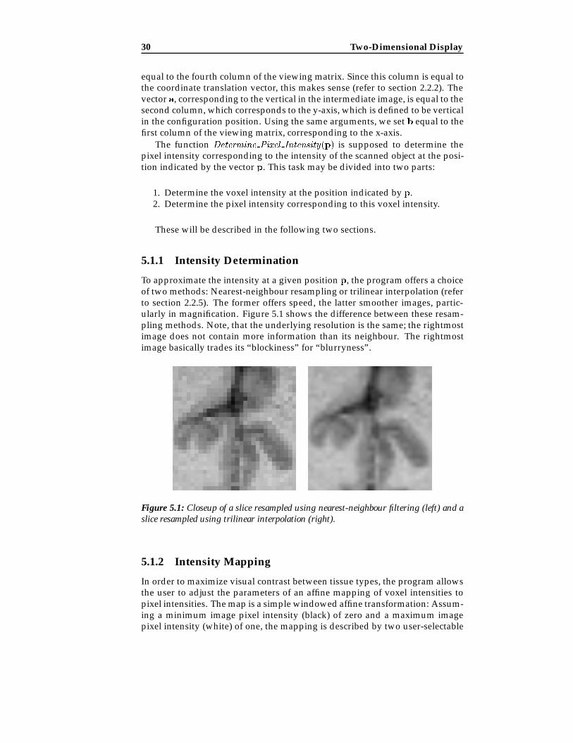
To approximate the intensity at a given position p, the program offers a choiceof two methods: Nearest-neighbour resampling or trilinear interpolation (referto section 2.2.5). The former offers speed, the latter smoother images, partic-ularly in magnification. Figure 5.1 shows the difference between these resam-pling methods. Note, that the underlying resolution is the same; the rightmostimage does not contain more information than its neighbour. The rightmostimage basically trades its “blockiness” for “blurryness”.
Figure 5.1: Closeup of a slice resampled using nearest-neighbour filtering (left) and aslice resampled using trilinear interpolation (right).
5.1.2 Intensity Mapping
In order to maximize visual contrast between tissue types, the program allowsthe user to adjust the parameters of an affine mapping of voxel intensities topixel intensities. The map is a simple windowed affine transformation: Assum-ing a minimum image pixel intensity (black) of zero and a maximum imagepixel intensity (white) of one, the mapping is described by two user-selectable
5.1 Rendering the intermediate image 31
1
w wh h
ip
ic
iv
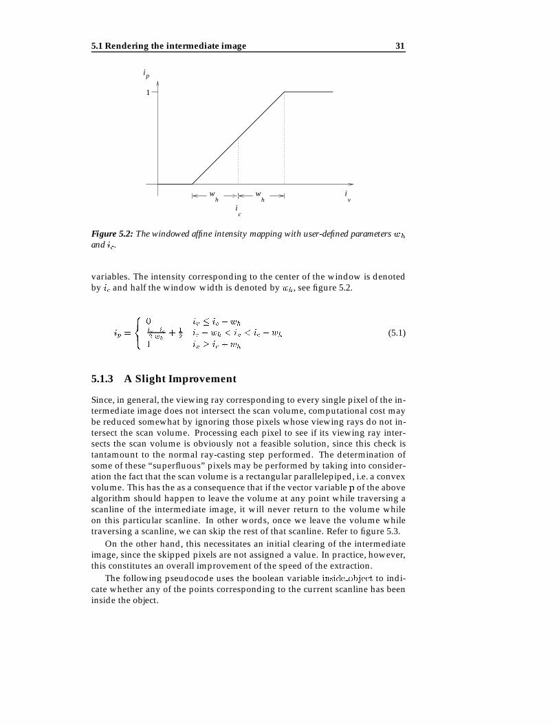
Figure 5.2: The windowed affine intensity mapping with user-defined parameters wh
and ic.
variables. The intensity corresponding to the center of the window is denotedby ic and half the window width is denoted by wh, see figure 5.2.
ip =
8<:
0 iv � ic � whiv�ic2 wh
+ 12 ic � wh < iv < ic + wh
1 iv � ic + wh
(5.1)
5.1.3 A Slight Improvement
Since, in general, the viewing ray corresponding to every single pixel of the in-termediate image does not intersect the scan volume, computational cost maybe reduced somewhat by ignoring those pixels whose viewing rays do not in-tersect the scan volume. Processing each pixel to see if its viewing ray inter-sects the scan volume is obviously not a feasible solution, since this check istantamount to the normal ray-casting step performed. The determination ofsome of these “superfluous” pixels may be performed by taking into consider-ation the fact that the scan volume is a rectangular parallelepiped, i.e. a convexvolume. This has the as a consequence that if the vector variable p of the abovealgorithm should happen to leave the volume at any point while traversing ascanline of the intermediate image, it will never return to the volume whileon this particular scanline. In other words, once we leave the volume whiletraversing a scanline, we can skip the rest of that scanline. Refer to figure 5.3.
On the other hand, this necessitates an initial clearing of the intermediateimage, since the skipped pixels are not assigned a value. In practice, however,this constitutes an overall improvement of the speed of the extraction.
The following pseudocode uses the boolean variable inside object to indi-cate whether any of the points corresponding to the current scanline has beeninside the object.

32 Two-Dimensional Display
Figure 5.3: Pixel skipping. This extracted intermediate image shows processed pixelsoutside the scan volume (black), and inside the scan volume (shades of gray) as well asskipped pixels (white).
inside object = falsefor v = 1 to h
for u = 1 to w
p = c+�u� w
2
�b+
�v � h
2
�a
if (p is inside the object) theninside object = trueImage(u; v) = Determine Pixel Intensity(p)
elseif (entered volume = true) then
inside object = falseSkip to next scanline
5.2 Applying the texture map
After extraction of the slice, the intermediate image needs to be registered as atexture to the graphics hardware. Following this, the texture map needs onlybe mapped to a quadrilateral. Ideally, this should be a 1:1 mapping, but sincethe user is allowed to resize the window (thus resizing the quadrilateral ontowhich the intermediate image is to be mapped), this is not always the case.This non-ideal mapping might lead to visual artifacts such as distinct pixeliza-tion, but since OpenGL is able to filter the texture appropriately (thus reducingartifacts to a minimum), this does not pose a problem.

5.3 Possible improvements 33
5.3 Possible improvements
It would be faster, and possible without significant loss of image quality, to letthe magnitude of a and b remain at unity (thus always performing slice ex-traction on a 1:1 scale which means zooming will not reduce the number ofskipped pixels) and then performing any zooming by enlarging the quadri-lateral onto which the two-dimensional intermediate image is mapped. Theadvantage of this method would be that is transfers the work of zooming fromthe CPU and onto the graphics hardware, thus freeing the CPU for other work.Obviously, for this to be an actual advantage, texture mapping hardware is re-quired. Using the appropriate texture filtering technique (nearest-neighbour orlinear interpolation, depending on the slice resampling filter) the image qualityloss would be negligible.
Another improvement would be to let the program use nearest-neighbourresampling while the user is interacting with the object and then render thegraphics using trilinear interpolation filtering when the interaction stops. Thisapproach will achieve good rendering speed during interaction and good im-age quality of static images.


Chapter 6
Three-DimensionalRendering
One of the problems of rendering two-dimensional images of three-dimensionalobjects is the sheer amount of data processing needed. One way of reducing therender time is commonly known as shear-warp rendering, briefly described insection 3.2. However, shear-warp rendering does just that: rendering. It leavesno information for the graphics library on how to handle the interaction of theshear-warp object and other graphics objects. Let us assume that we want toindicate with a polygon a certain planar slice of the three-dimensional object inquestion. Shear-warp rendering, by itself, generates no information on how tohandle the intersection of the polygon and the shear-warp object.
This chapter describes the implementation of three-dimensional renderingusing a shear-warp factorization of the viewing transformation, along withthe developed modifications for interactive display. Furthermore, a flexibleway of combining the aforementioned voxel-based rendering with conven-tional polygonal rendering is presented.
6.1 Shear-Warp Rendering
In order to achieve good performance on modern computers, it is important tokeep the data used in the fastest memory type possible. Since it is rarely possi-ble to keep all data in CPU registers alone, as much as possible should be keptin the fast data cache memory. This means focusing on small coherent portionsof memory instead of making spurious access of data at locations spread allover the memory at random. To achieve good cache coherency, an ideal vol-ume rendering method must perform in-order traversals of both volume and(screen) image data. Klein and Kubler [Klei85] proposed a method in whichthe view transformation matrix is factorized into a shear matrix and a warpmatrix. Using this factorization, rendering may be performed in four steps:
1. Choose the appropriate slicing direction. It is assumed that the volumedata may be sliced in three directions, each perpendicular to one of theworld space axes. In other words the voxels within each slice all have

36 Three-Dimensional Rendering
equal x-, y-, or z-coordinates. Choose the slicing direction such that thecorresponding set of slices is most perpendicular to the viewing direc-tion. The axis corresponding to this slicing direction is said to be theprincipal axis.
2. Shear (translate) each slice such that a viewing ray perpendicular to theset of slices in the sheared object space will intersect each slice in thesame manner as the oblique viewing ray would intersect the slices in un-transformed object space (see figure 3.2). This means, that in the shearedobject space, all viewing rays are parallel to the principal axis. To performa perspective transform, slices must be scaled as well as sheared.
3. Project the slices into a distorted 2D intermediate image in sheared objectspace. Since the shear coefficients are not confined to integers, properresampling is necessary to retain image quality.
4. Warp the intermediate image into image space, producing the correct fi-nal image.
The process of transforming the intermediate image into image space re-quires a general warp operation. However, since this is a 2D operation, the costis limited (about 10% of the total cost in typical cases, according to [Lacr95]).
Note, that the resampling used during the projection takes place in-slice.This potential problem of using a 2D rather than a 3D reconstruction filter toresample the volume data is discussed in section 6.4. The prototype allowsresampling using the 2D nearest-neighbour resampling filter or a bilinear filter,the latter being slightly slower owing to the fact that two voxel scanlines mustbe traversed simultaneously.
Assuming the volume consists of fully transparent and fully opaque vox-els only, the projection could be done using an approach akin to the paintersalgorithm: Projecting one sheared slice at a time in back-to-front order, newopaque voxels overwriting earlier (and thus more distant) voxels. Obviously,this would lead to a lot of overdraw in the typical case. It turns out to be ad-vantageous to project the slices front-to-back, ignoring any intermediate imagepixel once an opaque voxel has been projected onto it.
The factorization of the viewing transformation leads to a general warp anda simple shear operation. The advantage of this is the possibility of travers-ing each intermediate image scanline and each object volume scanline in syn-chrony, leading to maximum cache coherency, which in turn means maximumcache efficiency.
Note, that while it is possible to do each of the above steps “by hand” (onthe CPU), it is likewise possible to make use of the graphics hardware throughOpenGL in the final 2D warping stage of the process, thus relieving the CPUof this task. See section 6.2.
Since there are six principal viewing directions, two for each axis, it is possi-ble to achieve in-order object traversal by keeping one copy of the data volumecorresponding to each of these directions. However, relaxing the whole-objectin-order traversal constraint to in-order traversal of each slice, it is possible touse only half the amount of memory at a minute cost. This way, all slices aretraversed in-order, but the order in which the slices are traversed may changeto accommodate the front-to-back projection order (e.g. when the viewer is “be-hind” the object). Therefore, three copies of the volume are needed.
6.1 Shear-Warp Rendering 37
6.1.1 Spatial Coherency
Apart from the in-order traversal of both image space and object space, whatsets the shear-warp rendering method apart from other volumetric renderingmethods is its ability to exploit spatial coherency in both image space and ob-ject space. Images of human brains contain one coherent object, namely thebrain itself. This object space coherency leads to image space coherency.
One way of exploiting object space coherency would be to store voxel scan-lines as runs of voxels, e.g. “10 transparent voxels”, then “13 opaque voxels”.This is called run-length encoding[Fole97]. If object space coherency data isstored along with the object data in this way, the run-time transparency check-ing of each individual voxel is superfluous, since transparent voxels may beignored once and for all. Since typically 80% of the voxels of an MPR imageare transparent1, this constitutes significant savings in terms of run-time dataprocessing as well as storage space, since three run-length encoded copies areusually smaller than a single unprocessed volume.
However, preprocessing data by run-length encoding imposes severe limi-tations on the extent to which data may be changed on the fly (see section 6.3.6),since e.g. inserting an opaque pixel in a transparent run (thereby breaking upthe run) will necessitate a re-encoding of the volume.
Image space coherency may be exploited in a similar way. Recalling that,once a pixel has been set (i.e. once it has turned opaque) in the intermediateimage, it will not be changed again, it is possible to achieve a considerablespeed increase by keeping track of runs of opaque pixels in the intermediateimage. Assume that each opaque pixel is associated with a value that containsthe length of the rest of the current run. This way, it is possible to skip wholeruns of opaque pixels as well as the corresponding object voxel runs, since im-age space and object space are traversed in synchrony. However, when thefirst transparent pixel after an opaque run turns opaque, the length values ofthe whole run must be updated (since the length of the run just increased). In[Lacr95] it is shown, that path compression[Corm97] is a fast way of approximat-ing this update. Path compression is also the technique used in the prototypedescribed in this thesis.
6.1.2 The Shear-Warp Factorization
Assuming the z-axis is the principal axis (see section 6.1), the factorization maybe written[Lacr95]:
Mview = Mwarp �Mshear (6.1)
If the z-axis is not the principal axis, the viewing transformation matrix ispre-multiplied by a permutation matrix, see [Lacr95].
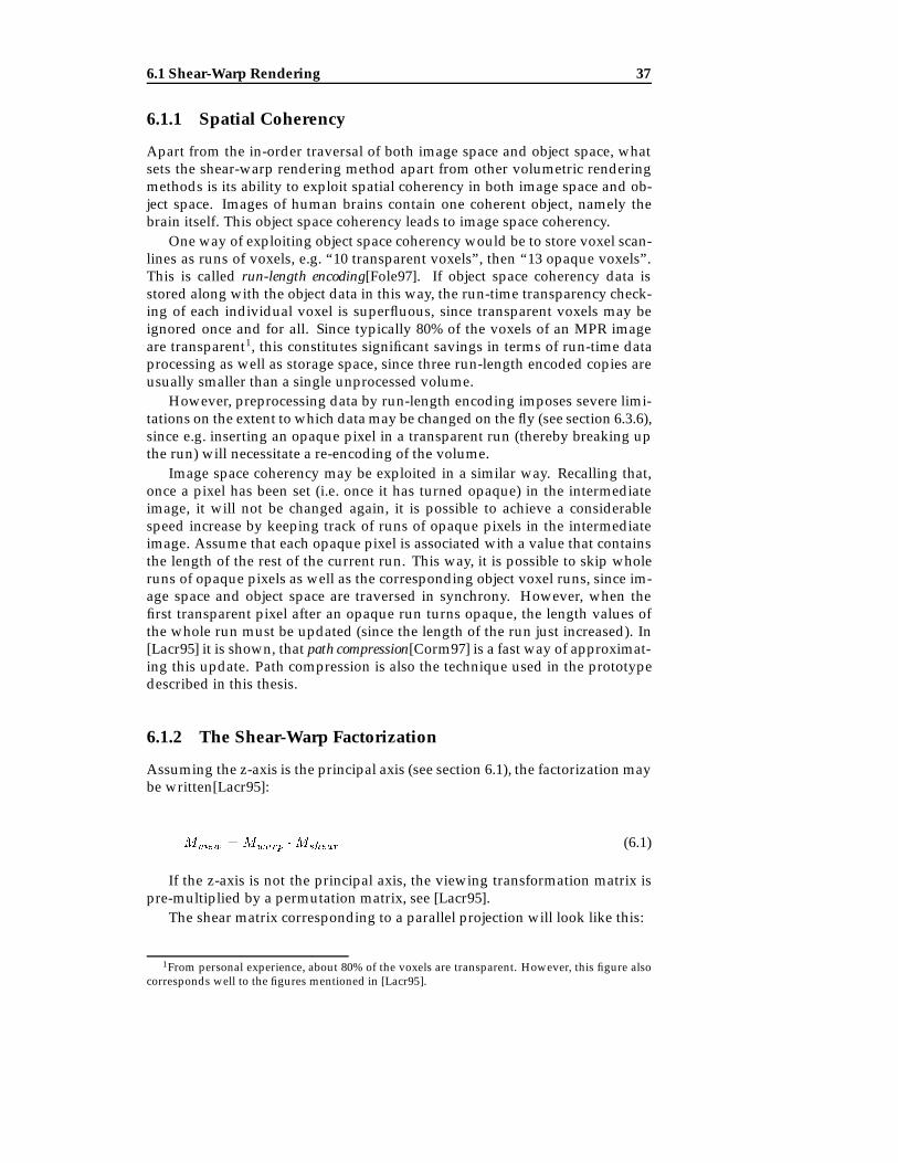
The shear matrix corresponding to a parallel projection will look like this:
1From personal experience, about 80% of the voxels are transparent. However, this figure alsocorresponds well to the figures mentioned in [Lacr95].
38 Three-Dimensional Rendering
Mshear =
2664
1 0 sx 00 1 sy 00 0 1 00 0 0 1
3775 (6.2)
where sx and sy denote the shear coefficients. Since this is always a regularmatrix, its inverse is well defined, and the warp matrix may be derived as:
Mwarp = Mview �M�1shear (6.3)
Once the principal axis has been determined, the shear coefficients are cho-sen such that all the viewing rays are parallel to the principal axis (refer tofigure 3.2). Subsequently, the slices are sheared using the shear matrix (6.2),projected and composited into the intermediate image. Finally, the intermedi-ate image is subjected to an affine warp by the warp matrix (6.3). The follow-ing sections describe how to take advantage of available hardware accelerationwhen warping and how to retain proper depth information, enabling appro-priate intersection of subsequently added polygonal graphics.
For more information on rendering using a shear-warp factorization of theviewing transformation, the reader is referred to [Lacr95].
6.2 Modifications for Interactive Display
Since the warp described in the previous section is an affine transformation,it is possible to perform the warp using the texture mapping feature of thegraphics library. As opposed to section 5.2, where a 1:1 mapping was desir-able, mapping the intermediate image as a texture onto a warped quadrilateralproduces the desired warpage. This is just a question of transforming the ver-tices of the quadrilateral using the warp matrix of equation (6.3). A polygonthus pretending to be a three-dimensional object is called an impostor.
6.3 Combining Voxels and Polygons
The problem of combining voxel-based graphics and polygonal graphics is thatof depth sorting. OpenGL uses the z-buffer (or depth buffer) technique, but itknows nothing about the depth information inherent in the rendered volume.It just “sees” a warped quadrilateral parallel to the image plane.
To solve this problem, proper depth information is generated and stored inthe z-buffer, thereby overwriting any earlier information. Therefore, the shear-warp object must be the first object being drawn in each frame.
6.3.1 Generating Depth Information
By modifying the inner loop of the shear-warp renderer to make a second in-termediate image which for each image pixel contains depth information ofthe corresponding voxel, it is possible to gain the depth information neededfor appropriate interaction with other objects.
6.3 Combining Voxels and Polygons 39
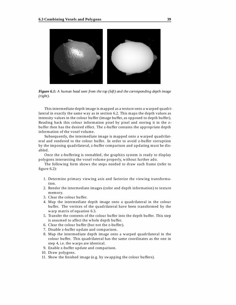
Figure 6.1: A human head seen from the top (left) and the corresponding depth image(right).
This intermediate depth image is mapped as a texture onto a warped quadri-lateral in exactly the same way as in section 6.2. This maps the depth values asintensity values in the colour buffer (image buffer, as opposed to depth buffer).Reading back this colour information pixel by pixel and storing it in the z-buffer then has the desired effect. The z-buffer contains the appropriate depthinformation of the voxel volume.
Subsequently, the intermediate image is mapped onto a warped quadrilat-eral and rendered to the colour buffer. In order to avoid z-buffer corruptionby the imposing quadrilateral, z-buffer comparison and updating must be dis-abled.
Once the z-buffering is reenabled, the graphics system is ready to displaypolygons intersecting the voxel volume properly, without further ado.
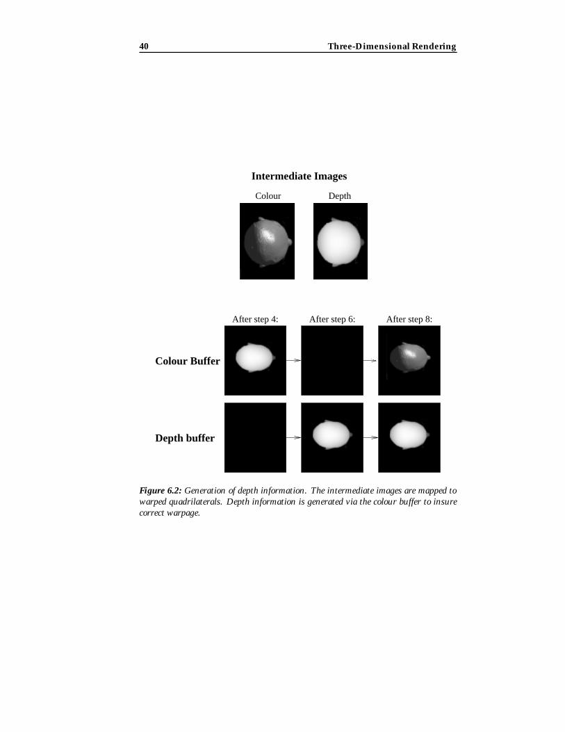
The following form shows the steps needed to draw each frame (refer tofigure 6.2):
1. Determine primary viewing axis and factorize the viewing transforma-tion.
2. Render the intermediate images (color and depth information) to texturememory.
3. Clear the colour buffer.4. Map the intermediate depth image onto a quadrilateral in the colour
buffer. The vertices of the quadrilateral have been transformed by thewarp matrix of equation 6.3.
5. Transfer the contents of the colour buffer into the depth buffer. This stepis assumed to affect the whole depth buffer.
6. Clear the colour buffer (but not the z-buffer).7. Disable z-buffer update and comparison.8. Map the intermediate depth image onto a warped quadrilateral in the
colour buffer. This quadrilateral has the same coordinates as the one instep 4, i.e. the warps are identical.
9. Enable z-buffer update and comparison.10. Draw polygons.11. Show the finished image (e.g. by swapping the colour buffers).
40 Three-Dimensional Rendering
Depth buffer
Colour Buffer
After step 4: After step 6: After step 8:
Colour Depth
Intermediate Images
Figure 6.2: Generation of depth information. The intermediate images are mapped towarped quadrilaterals. Depth information is generated via the colour buffer to insurecorrect warpage.

6.3 Combining Voxels and Polygons 41
Please note, that the depth image formed in step 4 is never shown directly,but transferred to the depth buffer. To see how such a depth image would look,refer to figure 6.1. Ideally, the intermediate image containing the depth imageshould be rendered directly to the depth buffer, but to the best of the author’sknowledge, OpenGL does not allow this.
The z-buffer must be disabled when performing step 8. Otherwise, the z-buffer contents would be overwritten with depth information correspondingto the imposing quadrilateral. If the impostor was behind the virtual objectrepresented by the z-buffer content, it would not be drawn at all.
Once the z-buffer contains the correct data corresponding to the shear-warpobject, any number of polygons may be added. Of significant use in this ap-plication would be a polygon indicating the position and orientation of thecurrent slice, see figure 6.3.
6.3.2 Limited buffer resolution
Since typical colour buffers use 8 bits precision per channel (red, green, blue,and opacity) the naıve implementation of the above would have a (maximum)z-buffer precision of 8 bits, and thus 256 equidistant depth values. Since these256 different depth positions are of the same order as magnitude as typicalscan volume resolutions, this limited precision does not pose a problem. Inthis section, however, a method to make the most of the limited resolution willbe presented.
Every element of the intermediate depth image is initialized to 255, whichwe define as the depth value corresponding to the far plane of the viewingfrustum. In order to get the most out of the limited precision, we map thedepth value of the nearest voxel to 0 and that of the most distant voxel to 254.Any depth value between these extremes is subject to an affine mapping. In thefollowing, this mapping will be referred to as depth coding, the result of whichis referred to as depth codes.
In practice, the depth values of the nearest and the most distant voxels,zmin and zmax, respectively, are found by examining the eight corners of thescan volume transformed into camera space.
The following affine transformation is then used to determine the depthcode zc of any depth value z between zmin and zmax:
zc = round
�254
z � zmin
zmax � zmin
�(6.4)
Before the buffer transfer step above (step 5) is performed, is it necessary totranslate the information of the colour buffer into proper depth buffer content.To do this, we need the z-axis distance of the near and far clipping planes,znear and zfar, respectively. In the default mode of OpenGL, a z-distance ofzfar corresponds to a depth buffer value of 1, whereas a z-distance of znearcorresponds to a depth buffer value of 0. Values between znear and zfar aresubject to an affine mapping.
Ignoring rounding errors, the depth of a pixel having depth code zc is equalto:

42 Three-Dimensional Rendering
z =
�zfar zc = 255
zc254 (zmax � zmin) + zmin zc < 255
(6.5)
Assume that the z-buffer assigns a value of zero to points whose z-componentis equal to znear and one to points whose z-component is equal to zfar. As-suming any voxel in question is inside the viewing frustum, the appropriatez-buffer value zz for a pixel corresponding to a voxel having a depth value ofz is
zz =z � znear
zfar � znear(6.6)
Thus, the appropriate z-buffer value zz for a pixel having depth code zc is:
zz =
(1 zc = 255
( zc254
(zmax�zmin)+zmin)�znearzfar�znear
zc < 255(6.7)
Remark: The current implementation does not work exactly the way described above.It uses a slightly different mapping to optimize for speed: The nearest and most distantpoints, zmin and zmax, are mapped to 1 and 255, respectively. The far clipping planezfar is mapped to zero. Using this mapping, clearing the intermediate depth image tozeroes (which can be done swiftly) leads to the desired initialization of the depth buffer.Furthermore, this mapping has the added benefit of enabling contour indication on theslice indication – see figure 6.3 and section 6.3.3.
To recapitulate the modified version of the above steps 2 through 5: Along-side the normal intermediate image, the modified shear-warp renderer createsan intermediate depth image, consisting of values translated into depth codesusing equation (6.4). This depth image is mapped onto a warped quadrilat-eral in a colour buffer. This colour buffer is read into system memory, and thecodes (pixel luminance) are converted back into approximate depth values us-ing equation (6.7). The colour buffer is cleared, and the depth values are thenstored in the z-buffer.
6.3.3 Contour Drawing
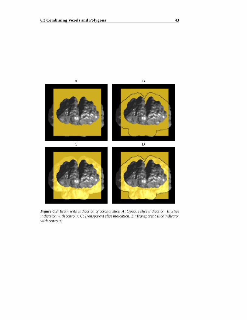
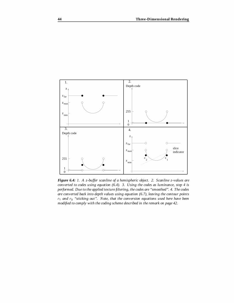
Figure 6.3 shows the frontal part of a brain peeking through a slice plane. Notehow the contour of the part of the brain behind the slice plane is visible. Thiscontour is actually an artifact caused by filtering the depth image when per-forming step 4 in section 6.3.1. Figure 6.4 shows how the contours come intoexistence. On figure 6.4.4, a slice indicator is placed. Since contour point c1 isin front of the slice indicator, it will “punch a hole” in it. The contour point c2,however, will not be visible, since the depth value of the slice indicator is lessthan that of the contour point. This shows that this method of contour draw-ing is less than perfect – but, after all, this contouring phenomenon is just anartifact, included as a curiosity, although it work quite well in practice. Note,that this contour drawing technique is based on the coding scheme describedin the remark in section 6.3.2.
6.3 Combining Voxels and Polygons 43
A B
C D
Figure 6.3: Brain with indication of coronal slice. A: Opaque slice indication. B: Sliceindication with contour. C: Transparent slice indication. D: Transparent slice indicatorwith contour.
44 Three-Dimensional Rendering
z
zmin
max
farz
z
1.Depth code
01
255
2.
Depth code
01
255
3.
z
zmin
max
farz
z
c2
c1
4.
sliceindicator
Figure 6.4: 1. A z-buffer scanline of a hemispheric object. 2. Scanline z-values areconverted to codes using equation (6.4). 3. Using the codes as luminance, step 4 isperformed. Due to the applied texture filtering, the codes are “smoothed”. 4. The codesare converted back into depth values using equation (6.7), leaving the contour pointsc1 and c2 “sticking out”. Note, that the conversion equations used here have beenmodified to comply with the coding scheme described in the remark on page 42.
6.3 Combining Voxels and Polygons 45
������������������������������������������������������������������������������������������������������������������������������������
������������������������������������������������������������������������������������������������������������������������������������
LN
R
Vθ θ y
z
z
xx
a
a
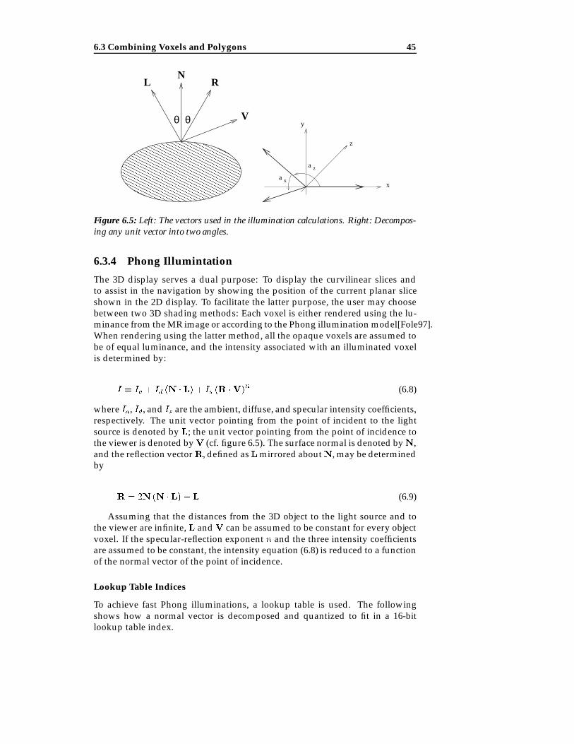
Figure 6.5: Left: The vectors used in the illumination calculations. Right: Decompos-ing any unit vector into two angles.
6.3.4 Phong Illumintation
The 3D display serves a dual purpose: To display the curvilinear slices andto assist in the navigation by showing the position of the current planar sliceshown in the 2D display. To facilitate the latter purpose, the user may choosebetween two 3D shading methods: Each voxel is either rendered using the lu-minance from the MR image or according to the Phong illumination model[Fole97].When rendering using the latter method, all the opaque voxels are assumed tobe of equal luminance, and the intensity associated with an illuminated voxelis determined by:
I = Ia + Id (N � L) + Is (R �V)n (6.8)
where Ia, Id, and Is are the ambient, diffuse, and specular intensity coefficients,respectively. The unit vector pointing from the point of incident to the lightsource is denoted by L; the unit vector pointing from the point of incidence tothe viewer is denoted byV (cf. figure 6.5). The surface normal is denoted byN,and the reflection vectorR, defined asLmirrored aboutN, may be determinedby
R = 2N (N � L) � L (6.9)
Assuming that the distances from the 3D object to the light source and tothe viewer are infinite, L andV can be assumed to be constant for every objectvoxel. If the specular-reflection exponent n and the three intensity coefficientsare assumed to be constant, the intensity equation (6.8) is reduced to a functionof the normal vector of the point of incidence.
Lookup Table Indices
To achieve fast Phong illuminations, a lookup table is used. The followingshows how a normal vector is decomposed and quantized to fit in a 16-bitlookup table index.

46 Three-Dimensional Rendering
A normal vector is a unit vector in three-dimensional space. Any such vec-tor may be constructed like so (cf. figure 6.5):
1. Start with the vector v = [1; 0; 0]T .2. Rotate v about the z-axis at an angle 0 � az � 180Æ.3. Then, rotate v about the x-axis at an angle 0 � ax < 360Æ.
Next, the angles ax and az are quantized such that
ax 2 f0; 1; 2; : : : ; 180g
az 2 f0; 1; 2; : : : ; 359g (6.10)
At this point, ax and az can easily be “wrapped” into a single integer ta asfollows:
ta = 360ax + az (6.11)
and unwrapped as follows:
ax =
�ta
360
�(6.12)
az = ta mod 360 (6.13)
The integer wrapping ta fits into a 16-bit unsigned integer, since, for any axand az satisfying equation (6.10), the following holds:
0 � ta � 65159 < 216 (6.14)
In practice
In the prototype, a preprocessing step (see section 9.2.2) calculates the normalvector corresponding to each voxel by normalizing the gradient approximationdescribed in section 2.2.4. This vector is then decomposed into the angles axand az which are subsequently quantized and wrapped into a 16-bit integerstored along with the intensity value of the corresponding voxel.
When rendering, ta is directly used as an index into a table of intensities,which must be recalculated with each frame2 using equation (6.8) for everycombination of the quantized angles ax and az given by the expression (6.10).
2More precisely: Table recalculation is necessary whenever object orientation changes relativeto light or viewer.

6.4 Disadvantages of Shear-Warp Rendering 47
6.3.5 Possible Improvements
To cater for the limited depth buffer resolution, another option would be to useseveral channels (red, green, blue, and opacity) for saving depth information.This way it would be possible to achieve up to 32 bits of depth buffer precision,which is more than most graphics hardware and libraries offer. Using thisapproach, it is essential to use a nearest-neighbour filter when mapping thedepth texture (step 4 above), since any kind of smoothing might corrupt thedepth information, depending on how the depth information is laid out in the4� 8 bits.
6.3.6 Alternatives
An alternative to this hassle of generating proper depth buffer data would be tovoxelize the polygons and let them be drawn together with the original shear-warp object. However, as seen in section 6.1.1, this would require run-lengthencoding the volume at every change of the orientation of any polygon rela-tive to the original voxel object (e.g. the brain). One way around this wouldbe to forgo the advantages of exploiting object space coherency and store theobject data in an unprocessed format. However, this still leaves the chore ofre-voxelising the polygons at each change of orientation or position, and thusre-traversing the volume. The method described in the previous sections al-lows quick graphical updates when changing polygon orientation, since the“artificially” generated z-buffer data does not change. In other words (assum-ing the generated z-buffer data is stored in a safe place): If any of the polygonschange (but the volumetric object does not), step 1 and 4 of the recipe of section6.3.1 may be skipped, along with the shear-warp rendering step itself.
6.4 Disadvantages of Shear-Warp Rendering
The disadvantage of shear-warp rendering is one concerning image quality.Since inter-slice filtering is not performed, “holes” may occur in the intermedi-ate image (and thus in the final image). With the understanding that the com-positing occurs in front-to-back order, this is illustrated in figure 6.6. Viewingray a is nearer to the transparent left pixel than the opaque right pixel in slice 0.Thus, passing slice 0 will not turn the pixel corresponding to this ray opaque.When passing slice 1, however, ray a is nearest to the opaque left pixel, andpixel a is set accordingly. Since both of the rays b and c are closer to the trans-parent pixels than to the opaque ones in both slices, the corresponding pixelsremain transparent, thus creating an undesired hole in the image. Note, thatthis artifact is independent of the resampling filter used, since resampling fil-ters only act on non-transparent voxels. In a full-fledged shear-warp rendererfeaturing semi-transparent voxels (such as the one in [Lacr95]), the problemwould be insignificant, since direct transitions from fully transparent to fullyopaque voxels (such as the ones in figure 6.6) are rare in typical MR data. Note,that, in practice, the problem only occurs when rendering “thin” objects, suchas voxelized surfaces, and not when rendering actually volumetric data. Seealso section 7.2.

48 Three-Dimensional Rendering
���������������������������������������������������������������������������������������������������������������������������������������������������������������������������������������������������������������������������������������
���������������������������������������������������������������������������������������������������������������������������������������������������������������������������������������������������������������������������������������
���������������������
���������������������
�������������������������������������������������������������������������������������������������������������������������
�������������������������������������������������������������������������������������������������������������������������
����������������
����������������
Image plane pixels
Slice 0
Slice 1
Viewing raysb c da
Figure 6.6: The disadvantage of shear-warp rendering: Holes may form when render-ing “thin” objects. Refer to section 6.4.

6.4 Disadvantages of Shear-Warp Rendering 49

Chapter 7
Curvilinear Reformatting
In order to automatically extract curvilinear slices as proposed by Bastos etal., it is necessary to determine the shape and location of the brain. This isequivalent to segmenting brain from non-brain tissue, which is exactly whatthe appropriately named Brain Extraction Tool (BET) from the Oxford Centrefor Functional Magnetic Resonance Imaging of the Brain does[Smit00]. BET isa part of the free1 FMRIB Software Library (FSL).
7.1 Brain Extraction Tool
BET reads a file containing a three-dimensional MR image, delineates the brainsurface and writes an MR image containing the brain only. However, in addi-tion to this brain-only image, BET is also able to output a brain mask, i.e. animage of the same dimensions as the original image, containing ones whereBET deems there be brain tissue, and zeros elsewhere.
To delineate the brain surface, BET starts by determining the parameters ofa “best-fit” sphere. This sphere is tesselated into a mesh of triangles, which issubsequently deformed to obtain a better fit. The deformation, which is doneiteratively until an optimal solution is found, takes two things into account:Fit quality and mesh smoothness. When a solution is found, an approxima-tive measure of self-intersection is applied. If this measure indicates that themesh most likely is self-intersecting, the whole process is repeated with strictersmoothness constraints.
7.2 Surface Extraction
Using the brain mask delivered by BET, it is possible to extract the outermostcurvilinear slice2 by selecting every voxel satisfying the following two condi-tions:
1. The voxel must be a brain tissue voxel according to the brain mask.
1Distributed under the GNU public license.2Note, this slice is not a unique set of voxels, but one depending on the employed notion of
connectivity.
52 Curvilinear Reformatting
2. At least one of the neighbours must be a non-brain voxel.
One way of extracting the next slice (the next layer of the analogous onion)would be to mark the previously extracted voxels as being non-brain voxelsand subsequently repeat the selection above.
However, to get, say, the eighth layer, one would have to perform eightiterations of selecting and re-marking. This is evidently inefficient, should onewant to access slices in a random order. See also section 7.3.
Another way would be to calculate for each brain tissue voxel the Euclideandistance to the nearest non-brain tissue voxel, and considering the results as afunction value or measure assigned to the voxels. The set of voxels having aEuclidean distance measure in a given interval would correspond to a slice ofa certain thickness. Once the distance calculation is done (needs only be doneonce), a single selection is all that is needed to extract any slice of any thickness.
Using this method, one could extract the eighth slice mentioned above byselecting those voxels whose distance measure was greater than seven and lessthan or equal to eight. Note, that the set of voxels of this slice would in gen-eral not be equal to the set extracted above, since connectivity has not beenconsidered, i.e. the meaning of “neighbour” has not been rigorously defined.
This method is the one employed in the prototype. Figure 7.1 shows fourslices extracted using this technique.
In order to avoid the problems associated with shear-warp rendering of thinsurfaces (see section 6.4), the program does not allow the display of single lay-ers (i.e. sets consisting of voxels of distance measure dlimit � 1 < dvoxel �dlimit+1). The selection phase only includes those voxels whose distance mea-sure is greater than a user-selected threshold. Thus, if the user set a distancethreshold value of zero, the selection phase includes all brain voxels.
The algorithm used to perform the Euclidean distance transformation isdue to Saito and Toriwaki[Sait93]. This algorithm calculates the exact dis-tance transform (as opposed to methods such as those employing the chamferalgorithm[Cars00]) of a 3D voxel volume in a matter of seconds on the devel-opment system.
Since the Euclidean distance (in voxels) between two voxel centers may bedetermined as
d(vijk ; vstu) =p
(s� i)2 + (t� j)2 + (u� k)2 (7.1)
the squared distance is always an integer. In the prototype, the squared dis-tance is the employed distance measure, since it saves the computation ofmany square roots and since integer comparisons are preferable to floatingpoint comparisons.
7.3 Other Metrics
In some cases, it may be advantageous to make use of other measures of dis-tance. Should one want to extract surfaces in the first way described in sec-tion 7.2, but without having to repeat the extraction to get subsequent layers,

7.3 Other Metrics 53
A B
C D
Figure 7.1: Curvilinear reformatting at varying distances from the surface. A: 2 mm.B: 4 mm. C: 8 mm. D: 12 mm.

54 Curvilinear Reformatting
one solution would be to perform a distance transform using the appropriatenotion of connectivity, i.e. calculating the distance from each object voxel tothe nearest (using the appropriate metric) non-object voxel. Assuming two-dimensional 4-connectivity3, this would mean calculating the distance trans-formation using the “city-block” metric. This distance transformation can beperformed swiftly using e.g. the chamfer algorithm[Cars00]. Defining a bor-der voxel to be an object voxel having a non-object voxel in its neighbourhood,selecting all voxels whose distance is d gives the exact same set of voxels asperforming the following:
iterate (d� 1) timesMark all border voxels.Turn marked voxels into (unmarked) non-object voxels
Select all border voxels.
This duality, which can be extended to other simple dual connectivity/metricpairs4, may be of some use due to the simplicity and the closeness to the layers-of-an-onion analogy, as well as the swiftness with which a distance transformsmay be performed.
3With 4-connectivity, the neighbours of a voxel at position (x; y) are (x� 1; y) and (x; y � 1).4Other pairs include the chess-board metric and 8-connectivity and equivalents in higher di-
mensions.

7.3 Other Metrics 55

Chapter 8
Dysplastic Lesion DetectionAid
In order to be able to detect dysplastic lesions of the cortex, it is necessaryto know what characterizes this abnormal tissue as opposed to normal tissue.Since MRI is the imaging method of choice, it would be particularly beneficialto know what MR imaging findings to expect when confronted with a dysplas-tic lesion.
As described in section 4.1.2, the aim is to detect cortical thickening and/orblurred gray matter / white matter junction. In order to detect cortical thicken-ing, a measure of cortical thickness is needed, which calls for the ability to tellcortical tissue from non-cortical tissue. However, according to the constraintsof section 4.1.2, any gray matter / white matter segmentation must be done bya trained expert. Here, a user-selected threshold is applied on the voxel inten-sities, which is not assumed to perform an accurate segregation of tissue typeson a voxel-wise basis, but is only intended to discard the set of voxels unlikelyto represent gray matter. This obviously calls for conservative thresholds.
8.1 Intensity Thresholding
Figure 8.1 shows part of a typical intensity histogram1 corresponding to anMPR image showing part of a human’s head. The histogram has has threehumps. The hump corresponding to the lowest voxel intensity derives mainlyfrom the background2, the middle hump mainly from gray matter and therightmost hump is due to white matter.
Judging from the histogram, the set consisting of brain voxels whose inten-sity is between 30 and 90 is very likely to contain a large proportion (if not all)of the gray matter voxels. Obviously, these thresholds are conservative, butprovide good initial threshold values.
Figures 8.3A and 8.3B show a planar slice before and after intensity thresh-olding.
1A conventional bar graph was unsuitable for the number of intensities, so a regular connected-line graph was used.
2The low-intensity voxels also derive from e.g. bone and CSF
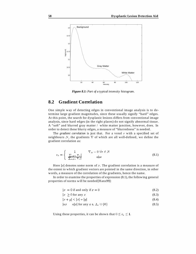
58 Dysplastic Lesion Detection Aid
20 40 60 80 100 120
10
10.5
11
11.5
12
12.5
13
Intensity
log(
coun
t)
Background
Gray Matter
White Matter
Figure 8.1: Part of a typical intensity histogram.
8.2 Gradient Correlation
One simple way of detecting edges in conventional image analysis is to de-termine large gradient magnitudes, since these usually signify “hard” edges.At this point, the search for dysplastic lesions differs from conventional imageanalysis, since hard edges (in the right places) do not signify abnormal tissue.A “soft” and blurred gray matter / white matter junction, however, does. Inorder to detect these blurry edges, a measure of “blurredness” is needed.
The gradient correlation is just that. For a voxel v with a specified set ofneighbours N , the gradients r of which are all well-defined, we define thegradient correlation as:
cv =
(1 rn = 0 8n 2 N
jP
n2Nrnj
Pn2N jrnj
else(8.1)
Here jxj denotes some norm of x. The gradient correlation is a measure ofthe extent to which gradient vectors are pointed in the same direction, in otherwords, a measure of the correlation of the gradients, hence the name.
In order to examine the properties of expression (8.1), the following generalproperties of norms will be needed[Hans99]:
jxj = 0 if and only if x = 0 (8.2)jxj � 0 for any x (8.3)jx+ yj � jxj+ jyj (8.4)jaxj = ajxj for any a 2 R+ [ f0g (8.5)
Using these properties, it can be shown that 0 � cv � 1.
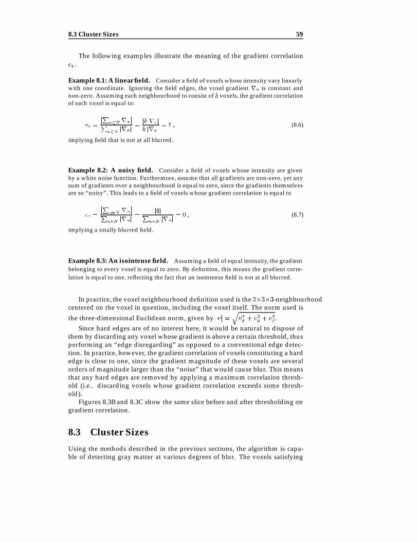
8.3 Cluster Sizes 59
The following examples illustrate the meaning of the gradient correlationcv .
Example 8.1: A linear field. Consider a field of voxels whose intensity vary linearlywith one coordinate. Ignoring the field edges, the voxel gradient rv is constant andnon-zero. Assuming each neighbourhood to consist of k voxels, the gradient correlationof each voxel is equal to:
cv =
��P
n2N rn
��
Pn2N jrnj =
jk rvjk jrvj = 1 ; (8.6)
implying field that is not at all blurred.
Example 8.2: A noisy field. Consider a field of voxels whose intensity are givenby a white noise function. Furthermore, assume that all gradients are non-zero, yet anysum of gradients over a neighbourhood is equal to zero, since the gradients themselvesare so “noisy”. This leads to a field of voxels whose gradient correlation is equal to
cv =
��P
n2N rn
��
Pn2N jrnj =
j0jP
n2N jrnj = 0 ; (8.7)
implying a totally blurred field.
Example 8.3: An isointense field. Assuming a field of equal intensity, the gradientbelonging to every voxel is equal to zero. By definition, this means the gradient corre-lation is equal to one, reflecting the fact that an isointense field is not at all blurred.
In practice, the voxel neighbourhood definition used is the 3�3�3-neighbourhoodcentered on the voxel in question, including the voxel itself. The norm used is
the three-dimensional Euclidean norm, given by jvj =qv2x + v2y + v2z .
Since hard edges are of no interest here, it would be natural to dispose ofthem by discarding any voxel whose gradient is above a certain threshold, thusperforming an “edge disregarding” as opposed to a conventional edge detec-tion. In practice, however, the gradient correlation of voxels constituting a hardedge is close to one, since the gradient magnitude of these voxels are severalorders of magnitude larger than the “noise” that would cause blur. This meansthat any hard edges are removed by applying a maximum correlation thresh-old (i.e.. discarding voxels whose gradient correlation exceeds some thresh-old).
Figures 8.3B and 8.3C show the same slice before and after thresholding ongradient correlation.
8.3 Cluster Sizes
Using the methods described in the previous sections, the algorithm is capa-ble of detecting gray matter at various degrees of blur. The voxels satisfying
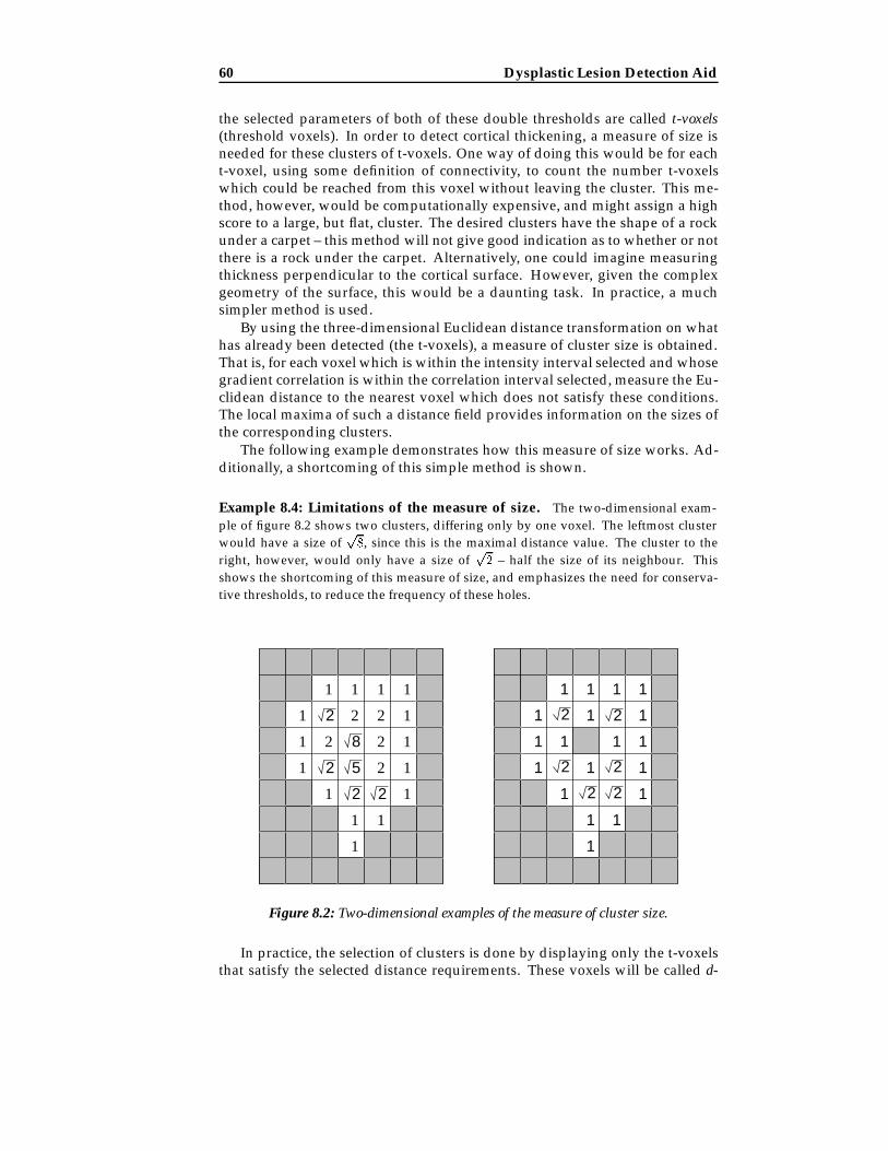
60 Dysplastic Lesion Detection Aid
the selected parameters of both of these double thresholds are called t-voxels(threshold voxels). In order to detect cortical thickening, a measure of size isneeded for these clusters of t-voxels. One way of doing this would be for eacht-voxel, using some definition of connectivity, to count the number t-voxelswhich could be reached from this voxel without leaving the cluster. This me-thod, however, would be computationally expensive, and might assign a highscore to a large, but flat, cluster. The desired clusters have the shape of a rockunder a carpet – this method will not give good indication as to whether or notthere is a rock under the carpet. Alternatively, one could imagine measuringthickness perpendicular to the cortical surface. However, given the complexgeometry of the surface, this would be a daunting task. In practice, a muchsimpler method is used.
By using the three-dimensional Euclidean distance transformation on whathas already been detected (the t-voxels), a measure of cluster size is obtained.That is, for each voxel which is within the intensity interval selected and whosegradient correlation is within the correlation interval selected, measure the Eu-clidean distance to the nearest voxel which does not satisfy these conditions.The local maxima of such a distance field provides information on the sizes ofthe corresponding clusters.
The following example demonstrates how this measure of size works. Ad-ditionally, a shortcoming of this simple method is shown.
Example 8.4: Limitations of the measure of size. The two-dimensional exam-ple of figure 8.2 shows two clusters, differing only by one voxel. The leftmost clusterwould have a size of
p8, since this is the maximal distance value. The cluster to the
right, however, would only have a size ofp2 – half the size of its neighbour. This
shows the shortcoming of this measure of size, and emphasizes the need for conserva-tive thresholds, to reduce the frequency of these holes.
2
22
2
2
2 2
2 2
2
8
1
1
11
1
1
1
22
1
1
2
1 1 1
1
1
1
25
1 1 1 1
1
1
1
1
1
1
1
1
1
1
1
1
1
1
1
2
Figure 8.2: Two-dimensional examples of the measure of cluster size.
In practice, the selection of clusters is done by displaying only the t-voxelsthat satisfy the selected distance requirements. These voxels will be called d-
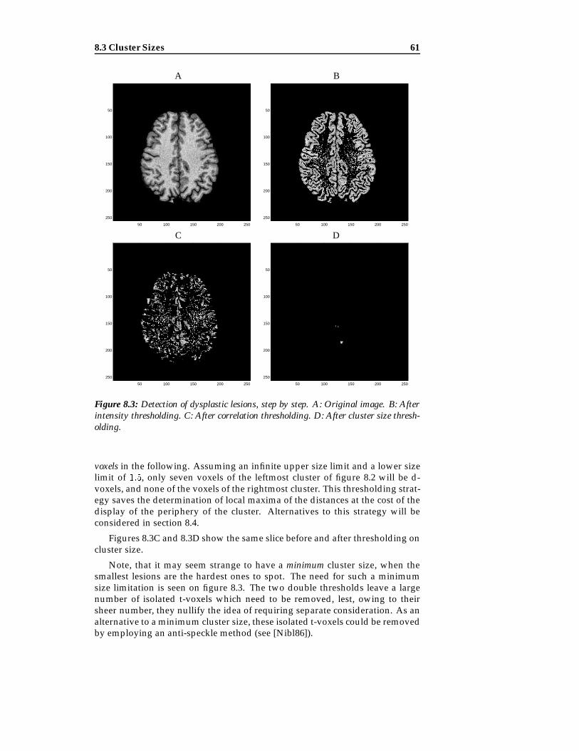
8.3 Cluster Sizes 61
A B
50 100 150 200 250
50
100
150
200
250
50 100 150 200 250
50
100
150
200
250
C D
50 100 150 200 250
50
100
150
200
250
50 100 150 200 250
50
100
150
200
250
Figure 8.3: Detection of dysplastic lesions, step by step. A: Original image. B: Afterintensity thresholding. C: After correlation thresholding. D: After cluster size thresh-olding.
voxels in the following. Assuming an infinite upper size limit and a lower sizelimit of 1:5, only seven voxels of the leftmost cluster of figure 8.2 will be d-voxels, and none of the voxels of the rightmost cluster. This thresholding strat-egy saves the determination of local maxima of the distances at the cost of thedisplay of the periphery of the cluster. Alternatives to this strategy will beconsidered in section 8.4.
Figures 8.3C and 8.3D show the same slice before and after thresholding oncluster size.
Note, that it may seem strange to have a minimum cluster size, when thesmallest lesions are the hardest ones to spot. The need for such a minimumsize limitation is seen on figure 8.3. The two double thresholds leave a largenumber of isolated t-voxels which need to be removed, lest, owing to theirsheer number, they nullify the idea of requiring separate consideration. As analternative to a minimum cluster size, these isolated t-voxels could be removedby employing an anti-speckle method (see [Nibl86]).
62 Dysplastic Lesion Detection Aid
8.4 Alternatives
Displaying the periphery of the t-voxel clusters would be an improvement,since the shape and the actual size of the cluster of t-voxels would be moreaccurately reproduced this way. This could be done by displaying any t-voxellocated in a cluster containing a d-voxel. Using conditional dilation [Serr88]this would be possible, but computationally expensive. A relatively cheap ap-proximation would be the following:
for each d-voxel vdisplay any voxel closer than dv to v
Here, dv denotes the distance from v to the nearest voxel that is not a t-voxelnor a d-voxel. Note, that a requirement that any voxels displayed be t-voxels isnot necessary. This might not give the correct shape of the cluster of t-voxels,but it does provide the general outline of the rock under the rug.
One could also consider improving the differential molecules used to es-timate the gradients and the neighbourhood used when measuring gradientcorrelation. Other filter kernels may be able to improve detection in some way,e.g. by reducing directional bias. The filter kernels chosen here are by no meansclaimed to be optimal; One should, however, be wary not to choose too largea kernel. Since the sought-after features are typically subtle, they are easilyeradicated by excessive smoothing.
8.5 Discussion
The lack of a third dimension inherent in computer screens and radiographicfilm imposes a severe handicap on a radiologist attempting to detect and lo-cate abnormal tissue in the brain. The radiologist is limited to a set of two-dimensional views of the data. Even if the object in question is derived from athree-dimensional data set, it is still projected onto a two-dimensional medium.The advantage of using a computer program to aid in the detection of dysplas-tic lesions lies in the fact that the algorithm is not restricted to two-dimensionalviews of the data.
Note how the method described in this chapter differs from conventional im-age analysis. Usually, one would attempt to find the sharpest edges in an image(e.g. road markings) or areas containing no edges (i.e. no obstructions); Here,the desired features, the blurred, soft edges, are somewhere in between. A de-fined, sharp transition from gray to white matter is usually a sign of healthytissue, whereas a blurred transition usually indicates abnormal tissue, such asa dysplastic lesion.
Although the three double thresholds (intensity, gradient correlation, and clus-ter size) are coupled, it is possible to shut out any one of them by suitable pa-rameter choices. For example, by setting the lower and upper gradient correla-tion thresholds to zero and one, respectively, the gradient correlation becomesdevoid of any importance.
8.5 Discussion 63
8.5.1 Non-Isotropic Voxels
This thesis has so far assumed voxels to be isotropic, i.e. having the same extentin all coordinate directions. Although the graphics subsystem does not havethis limitation, the detection aid and the curvilinear slice extraction discussedin this and the previous chapters would suffer from severe directional bias ifconfronted with (highly) anisotropic voxels.
In the case of the detection aid, the problem would be severe directional biascaused by the differential molecules employed to estimate image gradients.Correcting biased gradients is a question of multiplying each component of thegradient vectors by appropriate factors, i.e. factors inversely proportional tothe voxel size in the corresponding coordinate direction. Once the gradients arecorrected, the problem of rectifying the calculation of the gradient correlationremains. One way of doing this would be to associate weights (depending onthe distance to the center voxel v) to the gradients and gradient magnitudes ofequation (8.1), e.g. like a Gaussian filter kernel (see [Nibl86]), thus transformingthe unweighted sums in the numerator and denominator into weighted sums.
The cluster size thresholding and the curvilinear slice extraction both em-ploy the Euclidean distance transform, which must also be able to cope withthe anisotropy. Fortunately, the distance transformation is also convertible tothe anisotropic case. To quote [Sait93]:
[The proposed algorithms] are also applicable with slight modifi-cation to a digitized picture sampled with the different samplinginterval in each coordinate axis.
According to said article, the distance transform can be adapted to typical 3DMR images, where voxels are larger in the coordinate direction perpendicularto the slice, without any difficulty.
Although the method developed in this thesis is aimed at (near-) isotropic datasets, it can be modified to the general case without much trouble by followingthe above guidelines.
8.5.2 Blur Versus Noise
Since the noise level in 3D MR images is rather high, it may be difficult todifferentiate the noise arising from structural changes in the cortex (such as“bizarre cells”) from the noise also present in MR images of normal subjects.This latter noise type arises from patient motion (gross patient motion, respi-ratory motion and motion caused by pulsatile blood flow), scanner hardware,and the employed MR acquisition technique. In a particularly noisy image, thegray matter / white matter junction may seem blurred all over. Whereas thehuman vision system may be able to detect differences in the noise types, thismay not be the case for the automated system described in this chapter. Whenusing the developed method and encountering a highly noisy MR image, itmay be necessary to disregard the blurring altogether and focus on detectingother symptoms. At the time of writing, the author has had no opportunity totest the method on a severely noisy MR image.

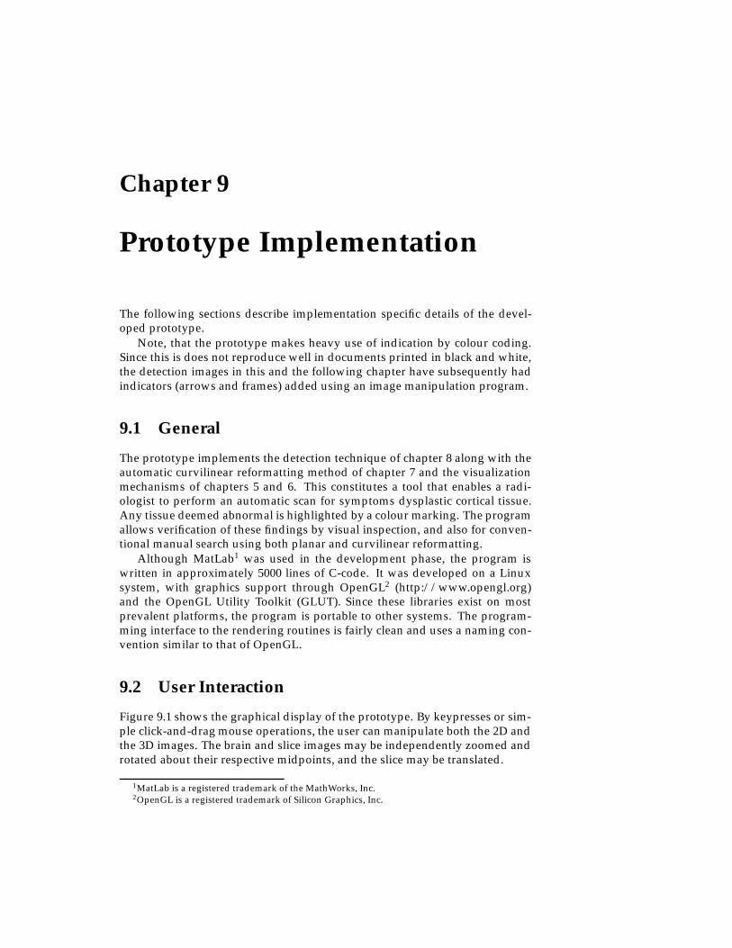
Chapter 9
Prototype Implementation
The following sections describe implementation specific details of the devel-oped prototype.
Note, that the prototype makes heavy use of indication by colour coding.Since this is does not reproduce well in documents printed in black and white,the detection images in this and the following chapter have subsequently hadindicators (arrows and frames) added using an image manipulation program.
9.1 General
The prototype implements the detection technique of chapter 8 along with theautomatic curvilinear reformatting method of chapter 7 and the visualizationmechanisms of chapters 5 and 6. This constitutes a tool that enables a radi-ologist to perform an automatic scan for symptoms dysplastic cortical tissue.Any tissue deemed abnormal is highlighted by a colour marking. The programallows verification of these findings by visual inspection, and also for conven-tional manual search using both planar and curvilinear reformatting.
Although MatLab1 was used in the development phase, the program iswritten in approximately 5000 lines of C-code. It was developed on a Linuxsystem, with graphics support through OpenGL2 (http://www.opengl.org)and the OpenGL Utility Toolkit (GLUT). Since these libraries exist on mostprevalent platforms, the program is portable to other systems. The program-ming interface to the rendering routines is fairly clean and uses a naming con-vention similar to that of OpenGL.
9.2 User Interaction
Figure 9.1 shows the graphical display of the prototype. By keypresses or sim-ple click-and-drag mouse operations, the user can manipulate both the 2D andthe 3D images. The brain and slice images may be independently zoomed androtated about their respective midpoints, and the slice may be translated.
1MatLab is a registered trademark of the MathWorks, Inc.2OpenGL is a registered trademark of Silicon Graphics, Inc.

66 Prototype Implementation
Figure 9.1: Screenshot of the graphics display. On the left is the 3D display with aslice indicator. On the right is the 2D slice.
The display of curvilinear slices mainly affects the 3D display. However, acurve indicating the intersection between the curvilinear slice and planar sliceis shown on the 2D display (see figure 9.2). This curve is updated wheneverthe user selects a different curvilinear slice. Curvilinear reformatting may beturned on or off.
The display of detections, shown in figure 9.2, can be turned on or off.When on, the detections are shown on both the 2D and 3D displays, includ-ing curvilinear slices. After adjusting detection parameters (the double thresh-old values on intensity, correlation, and cluster size), the user may start a re-detection.
To enable user control of the image contrast, the user may adjust the pa-rameters of the intensity mapping described in section 5.1.2. The adjustmentis performed by dragging the mouse while holding down the middle mousebutton, which is the de facto standard of contrast control in e.g. MPR software.
The resampling method employed is selected at a keypress.Sections 9.3 and 9.4 describes two extra features that may ease the detection
of cortical disorders.
9.2.1 Selective Updating
By only recalculating and redrawing when necessary, it is possible to save aconsiderable amount of data processing, which in turn leads to a higher rateof graphical updating. By saving intermediate images as well as depth infor-mation, much work can be saved, since e.g. rotating the planar slice does notrequire retraversal of the three-dimensional MR image, even though the sliceindicator on the 3D display would need to be updated.
The following table describes the necessary updates corresponding to a gi-ven user action.
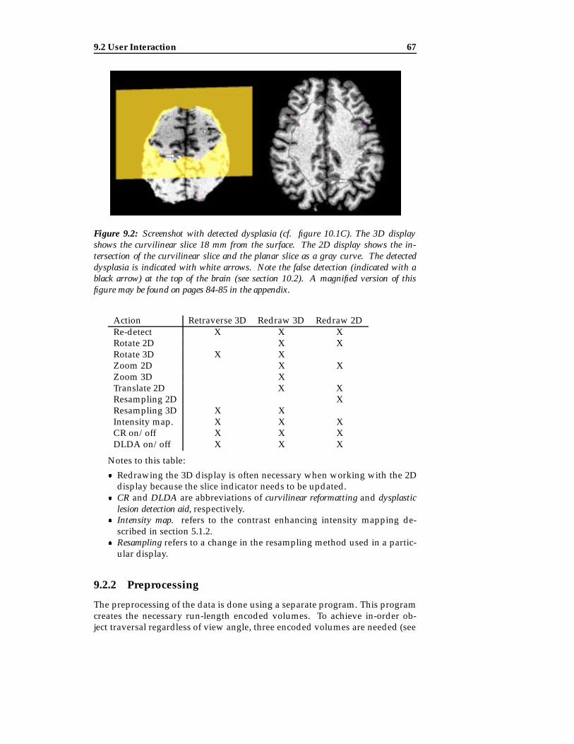
9.2 User Interaction 67
Figure 9.2: Screenshot with detected dysplasia (cf. figure 10.1C). The 3D displayshows the curvilinear slice 18 mm from the surface. The 2D display shows the in-tersection of the curvilinear slice and the planar slice as a gray curve. The detecteddysplasia is indicated with white arrows. Note the false detection (indicated with ablack arrow) at the top of the brain (see section 10.2). A magnified version of thisfigure may be found on pages 84-85 in the appendix.
Action Retraverse 3D Redraw 3D Redraw 2DRe-detect X X XRotate 2D X XRotate 3D X XZoom 2D X XZoom 3D XTranslate 2D X XResampling 2D XResampling 3D X XIntensity map. X X XCR on/off X X XDLDA on/off X X X
Notes to this table:
� Redrawing the 3D display is often necessary when working with the 2Ddisplay because the slice indicator needs to be updated.
� CR and DLDA are abbreviations of curvilinear reformatting and dysplasticlesion detection aid, respectively.
� Intensity map. refers to the contrast enhancing intensity mapping de-scribed in section 5.1.2.
� Resampling refers to a change in the resampling method used in a partic-ular display.
9.2.2 Preprocessing
The preprocessing of the data is done using a separate program. This programcreates the necessary run-length encoded volumes. To achieve in-order ob-ject traversal regardless of view angle, three encoded volumes are needed (see

68 Prototype Implementation
Figure 9.3: Emphasizing the cortical structure facilitates detection of abnormal corticalasymmetries (black frame).
section 6.1.1). The program accepts a user-selected threshold and classifies allvoxels as being transparent (if their intensity is below the threshold) or opaque(if their intensity is above the threshold). The gradients of all opaque voxels arethen calculated, encoded (see section 6.3.4), and stored along with the intensityof the corresponding voxel in each of the three run-length encoded volumes.The gradient correlation corresponding to each voxel is also calculated andstored in a separate file.
9.3 Histogram Display
To aid in the determination of feasible parameters for the intensity thresholds,the program features the display of intensity histograms (see figure 8.1). Theuser can zoom in and out on any parts of the histogram by clicking the mousebuttons. This histogram, which is drawn as a connected-line graph, may helpthe user find feasible parameters by showing the approximate ranges of mainvoxel types (background, gray matter, and white matter).
9.4 Cortical Detection
In order to emphasize the cortical structure, the prototype contains a simplemethod of detecting gray matter. The method uses the same parameters as thedysplastic lesion detection method, but in a different way:
1. Select all voxels whose intensity is within the range of the user-selectedintensity thresholds.
2. Remove all voxels whose gradient correlation is below the upper correla-tion threshold. This ensures that only gray matter matter near an edge
9.5 Data 69
(background / gray matter edge or gray matter / white matter edge) areincluded. The voxels that pass steps 1 and 2 are called b-voxels.
3. Discard the b-voxels, whose 3 � 3 � 3-neighbourhood contains less thanbmin b-voxels, where bmin is a user-selected threshold. This last step re-moves isolated voxels and small clusters of voxels which may distract theradiologist.
Figure 9.3 shows how putting visual emphasis on cortical structure facili-tates the visual detection of cortical asymmetry.
An alternative would have been to use a more advanced and accurate seg-mentation tool, such as FMRIB’s Automated Segmentation Tool (see section10.2). FAST takes about 45 minutes segmenting a standard MR image on thefastest settings, and even that is considered fast in the field of automated tis-sue segmentation. Since the prototype is supposed to be an interactive tool,advanced segmentation techniques are thus out of the question.
It should be noted, that the cortical detection algorithm described in thissection does not perform a voxel-wise tissue segmentation. It only approx-imates the cortical structure so as to be able to emphasize it for facilitatingdetection of asymmetry of the cortical structure.
9.5 Data
The preprocessing program and the main part of the prototype are both capa-ble of reading data in the simple file and Analyze formats, provided the inten-sity values be represented using 16-bit signed integers using little-endian byteordering or 32-bit ieee floating point numbers. Internally, intensities are repre-sented using 16-bit signed integers.
The loaded data consists of:
� Three run-length encoded volume files (containing intensity and gradi-ent information), each corresponding to a principal slicing direction.
� One (unencoded) volume file containing voxel intensities, used for pla-nar slicing and display.
� One (unencoded) volume file containing gradient correlation.� One (unencoded) brain mask (generated by Brain Extraction Tool).
The gradient correlation file is optional, as is the brain mask. However,without the gradient correlation, automatic symptom detection is disabled,and without the brain mask, curvilinear reformatting is disabled.
Each of the above four items represent approximately 18 megabytes of datafor a 256�256�140voxel volume, totalling 72 megabytes of data loaded whenoptional features are enabled.
9.6 Performance and Requirements
The main program allocates 18 to 20 bytes per voxel loaded, plus an additional7 Mb for textures and intermediate storage. This means that, using a normal
70 Prototype Implementation
256 � 256 � 140 voxel volume as data source, the program takes up approxi-mately 180 megabytes of memory.
On the development computer, an AMD 1.3 GHz CPU equipped systemwith 512 megabytes of RAM, the rendering speed was about 3 frames per sec-ond when simultaneously updating both displays. This is barely enough forhassle-free interaction.
The development system is equipped with a graphics card capable of ac-celerating OpenGL graphics in hardware. Although OpenGL is only used todraw three texture mapped quadrilaterals (2d, 3d, and depth images) as wellas for one colour buffer read operation and one depth buffer write operation,hardware acceleration has significant impact on frame rates.
In the current implementation, the OpenGL driver takes by far the largestportion of the frame time:
60% of the frame time is used by the OpenGL driver performing the colourbuffer read and the depth buffer write.
25% of the frame time is used by the OpenGL driver uploading the appropri-ate textures to graphics memory.
This leaves only 15% of the frame time for everything else, such as travers-ing the volume to form the intermediate images, converting depth informa-tion, etc. The OpenGL buffer reads/writes are notoriously slow, in part be-cause a graphics pipeline flush and stall are needed. Although most moderngraphics hardware supports it, there is not yet a render-to-texture mechanismin OpenGL3. By optimizing these issues alone (e.g. by performing the warpedmapping in software, thus bypassing the driver), frame rates in the twentiesare estimated to be achievable on the development system.
Updating the array of detected voxels after a change of parameters takesabout 10 seconds on the development system. A slight improvement mayexpected to arise from optimizing the distance transform implementation forspeed.
At a slight cost in speed, memory consumption may also be approximatelyhalved by packing data in a more efficient manner. As an example: Each voxelin the brain mask contains one bit of information (brain/non-brain), yet itsinternal format is 16-bit signed integer.
3Sadly, even the OpenGL version 1.3 specifications released 14th of August 2001 contain norender-to-texture feature.

9.6 Performance and Requirements 71

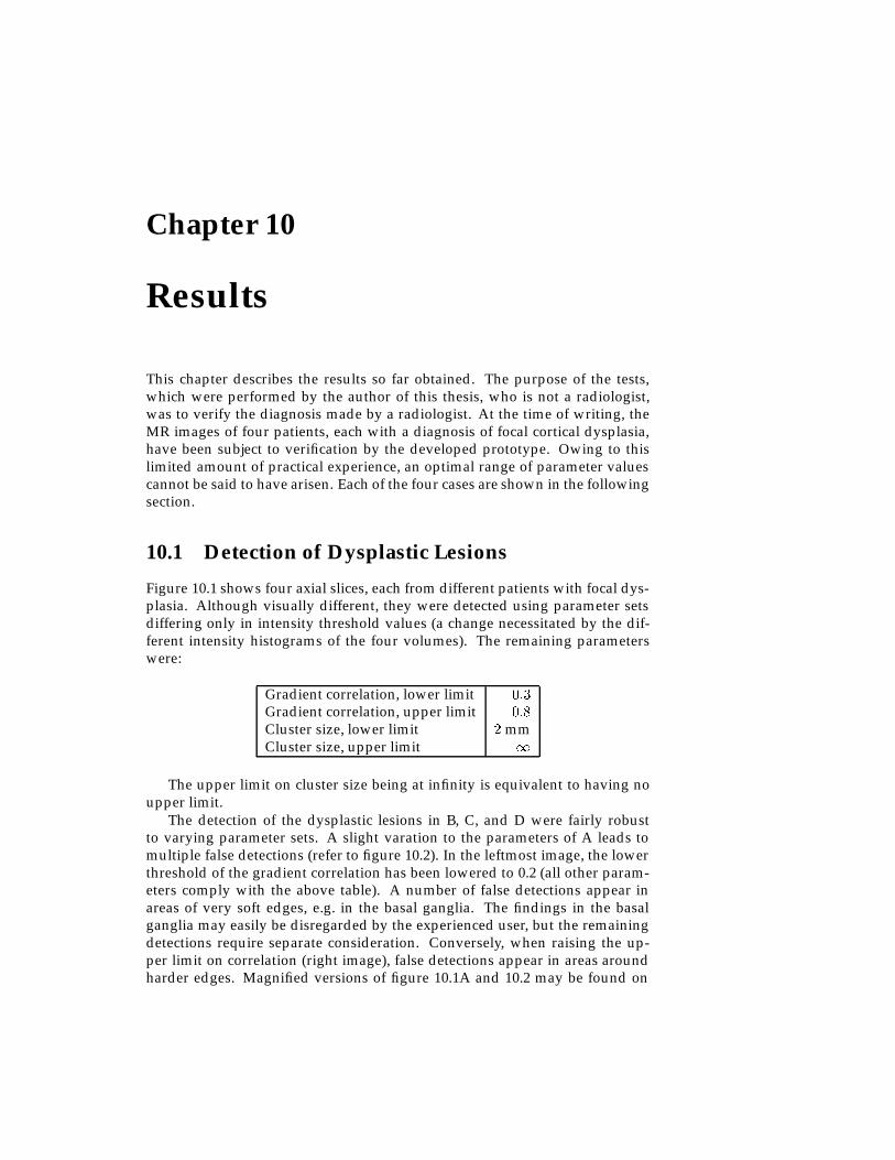
Chapter 10
Results
This chapter describes the results so far obtained. The purpose of the tests,which were performed by the author of this thesis, who is not a radiologist,was to verify the diagnosis made by a radiologist. At the time of writing, theMR images of four patients, each with a diagnosis of focal cortical dysplasia,have been subject to verification by the developed prototype. Owing to thislimited amount of practical experience, an optimal range of parameter valuescannot be said to have arisen. Each of the four cases are shown in the followingsection.
10.1 Detection of Dysplastic Lesions
Figure 10.1 shows four axial slices, each from different patients with focal dys-plasia. Although visually different, they were detected using parameter setsdiffering only in intensity threshold values (a change necessitated by the dif-ferent intensity histograms of the four volumes). The remaining parameterswere:
Gradient correlation, lower limit 0:3Gradient correlation, upper limit 0:8Cluster size, lower limit 2 mmCluster size, upper limit 1
The upper limit on cluster size being at infinity is equivalent to having noupper limit.
The detection of the dysplastic lesions in B, C, and D were fairly robustto varying parameter sets. A slight varation to the parameters of A leads tomultiple false detections (refer to figure 10.2). In the leftmost image, the lowerthreshold of the gradient correlation has been lowered to 0.2 (all other param-eters comply with the above table). A number of false detections appear inareas of very soft edges, e.g. in the basal ganglia. The findings in the basalganglia may easily be disregarded by the experienced user, but the remainingdetections require separate consideration. Conversely, when raising the up-per limit on correlation (right image), false detections appear in areas aroundharder edges. Magnified versions of figure 10.1A and 10.2 may be found on

74 Results
A B
C D
Figure 10.1: Detected focal dysplasias verified by a radiologist. Dysplastic lesions areframed.
pages 86–88 in the appendix.
Unfortunately, the prototype has as yet been used only to verify previouslymade diagnoses – the acid test of actually making a diagnosis awaits the nearfuture.
10.2 Effects of Intensity Nonuniformity
Owing to inhomogeneous receiver coil sensitivity, inhomogeneous main fieldand RF field, and inhomogeneous magnetic susceptibility (“magnetizability”)of the scanned object, spatial intensity variation unrelated to the anatomicstructure may arise. This variation, or bias, typically leads to a clearly visibledecrease in intensity level and tissue contrast at the top and bottom of sagittal

10.2 Effects of Intensity Nonuniformity 75
Figure 10.2: Axial slices demonstrating the effects of parameter variation in patient A.Left: Lower correlation threshold set to 0:2. Right: Upper correlation threshold set to0:9. The dysplasia is indicated with white arrows, false detections with black arrows.Magnified versions of these images can be found on pages 87-88 of the appendix.
Figure 10.3: Sagittal (left) and coronal slices showing false detections caused by in-tensity nonuniformity. Magnified versions of these can be found on page 89 of theappendix.

76 Results
and coronal views. Whereas the decrease in intensity level may not have greatsignificance on the visual interpretation of brain images, the results of compu-tational procedures may suffer a great deal. This type of nonuniformity maybe seen as a “shadow” at the top of the brain depicted in figure 7.1.
For the following two reasons, the method described in this thesis can beexpected to have a significant amount of false detections when used on suchnonuniform images:
� The general decrease in intensity makes white matter voxels have lumi-nance values in the gray matter area, so that everything seems to be graymatter.
� The decrease in tissue contrast gives rise to a decrease in the signal-to-noise ratio, making every remaining edge seem fuzzy.
This expectation proves to hold in practice: figure 10.3 shows a considerableamount of false detections due to image bias. Note, that the false detection onfigure 9.2 is also caused by this kind of intensity nonuniformity.
The FMRIB software library (from where Brain Extraction Tool originates)contains a tissue segmentation program capable of performing for bias correc-tion. This program, called FAST (FMRIB’s Automated Segmentation Tool, see[Zhan00]), has been used to correct a biased image. Unfortunately, the numberof false detections did not decrease significantly using this corrected image,most probably because the tissue contrast in the parts of the original imageaffected the most by this bias had already inreparably deteriorated.
A comprehensive evaluation of nonuniformity correction methods can befound in [Arno01].

10.2 Effects of Intensity Nonuniformity 77


Chapter 11
Summary
Manual detection of the development disorder of the cerebral cortex, known asfocal cortical dysplasia (FCD), may take several days of combing through mag-netic resonance (MR) data, even for a clinical expert. An algorithm to assist inthe detection by 3D image analysis has been presented. This algorithm detectstwo key symptoms of FCD, namely thickening of the cortex and poor differen-tiation of gray matter versus white matter. To facilitate manual verification ofdetections, the algorithm has been embedded in a graphics system combiningconventional planar as well as curvilinear slice view to facilitate interpretationof data. A strong point in the algorithm is the fact that it is three-dimensionalin nature, as opposed to the inspection by a human user, who is restricted toexamining a few two-dimensional surfaces at a time. It should be noted, how-ever, that the method presented here constitutes a tool for assisting a clinicalexaminer, and not for automatically making diagnoses.
The results so far are few, but encouraging.
11.1 Main Contributions
In summary, the main contributions of this thesis are as follows:
� A method for fast automatic detecting of key symptoms of focal corticaldysplasia.
� Automation of the type of curvilinear reformatting introduced in [Bast99].� Extension of the shear-warp rendering method to achieve the appropriate
behaviour when interacting with subsequently added graphical objects.� Demonstration of the use of texture mapping hardware to perform the
affine 2D warp required by shear-warp rendering.
11.2 Possible Improvements
The method reports a fair amount of noise as well as some strong false find-ings. The former is characterized by the erroneous detection of small clusters

80 Summary
(typically consisting of a single voxel) and most may be disregarded when tak-ing their size into consideration. The latter are caused by the following:
� Restricting the program to consider local geometry information only; tohave no knowledge of the global tissue anatomy. False detections in thebasal ganglia (also consisting of gray matter), for example, belong to thisclass
� Intensity nonuniformity. This is easily identified as a general decrease inintensity and contrast
If these types of false findings are disregarded, the remaining detectionsare usually few, and may be accepted or rejected manually. Whether or notexperience will teach radiologists to unconsciously disregard the false findingsof these types, only time will tell.
The program has been assessed by a radiologist, and general navigationand positioning of slices was found to cause inconvenience. A few simple nav-igational tools were suggested to solve the problem, see section 11.4.
11.3 Benefits
The method is able to detect visually different dysplastic lesions using the sameset of parameters. Using other parameter sets, it should be possible to facilitatethe detection of other abnormalities such as tumours and subtle cerebral hem-orrhages. The algorithm uses simple (and thus fast) image analysis techniquesand may easily be extended to detect other features.
By being an inherently three-dimensional algorithm, it is capable of help-ing a radiologist “see through” the flat images on a computer screen, therebyreducing the effect of the reduced dimensionality of conventional MR analysistools.
The graphics system, having a 2D as well as a 3D image with indication ofcontours and trouble spots is reported as being “very appealing”.
11.4 Future Work
Obviously, the method still needs much testing in order to pin down feasibleparameter ranges, as well as to provide the radiologist with the experienceneeded to swiftly discern different classes of findings. Further issues of futurework include:
� Tools for orientation. A simple indication of the object coordinate systemwas suggested, as well as a means of correlating the images of the 2D and3D displays.
� Reducing the number of false detections.� Optimizing other parameters, such as the filter kernels and differential
molecules.� Extending the algorithm to provide valid results for data volumes con-
sisting of non-isotropic voxels.

11.5 Conclusion 81
� Optimizing the graphics system for speed. A dramatic increase is as-sumed possible.
� To let graphics hardware perform the 2D zooming as described in section5.3.
� To sacrifice imaging quality for speed when interacting with the object,and then to render at maximum quality once the interaction stops (alsodescribed in section 5.3).
� To introduce alternative measures of cluster size to improve the detec-tion of cortical thickening regardless of shape and natural variations incortical thickness.
� Displaying the periphery of detected clusters to emphasize cluster sizesand shapes.
� By finding local maxima in the distance-to-nearest-non-t-voxel volume,the approximate size and location of dysplasias can be determined. Thisway, the program would be able to lead the radiologist directly to thestrongest detections.
11.5 Conclusion
The object of this work reported here was to develop a tool to assist a radiolo-gist in the localization of subtle focal cortical dysplastic lesions. An algorithmcapable of detecting key symptoms of such disorders was developed alongwith a graphics system to support verification of findings by visual inspection.Much experimental work is needed to determine whether or not the method isvaluable, yet the results so far are encouraging.
The development continues.


Appendix A
Selected Images
This following pages contain blow-ups of the more detailed images of this the-sis. The images have been enhanced using an image manipulation program tocompensate for the lack of colour in this reproduction.
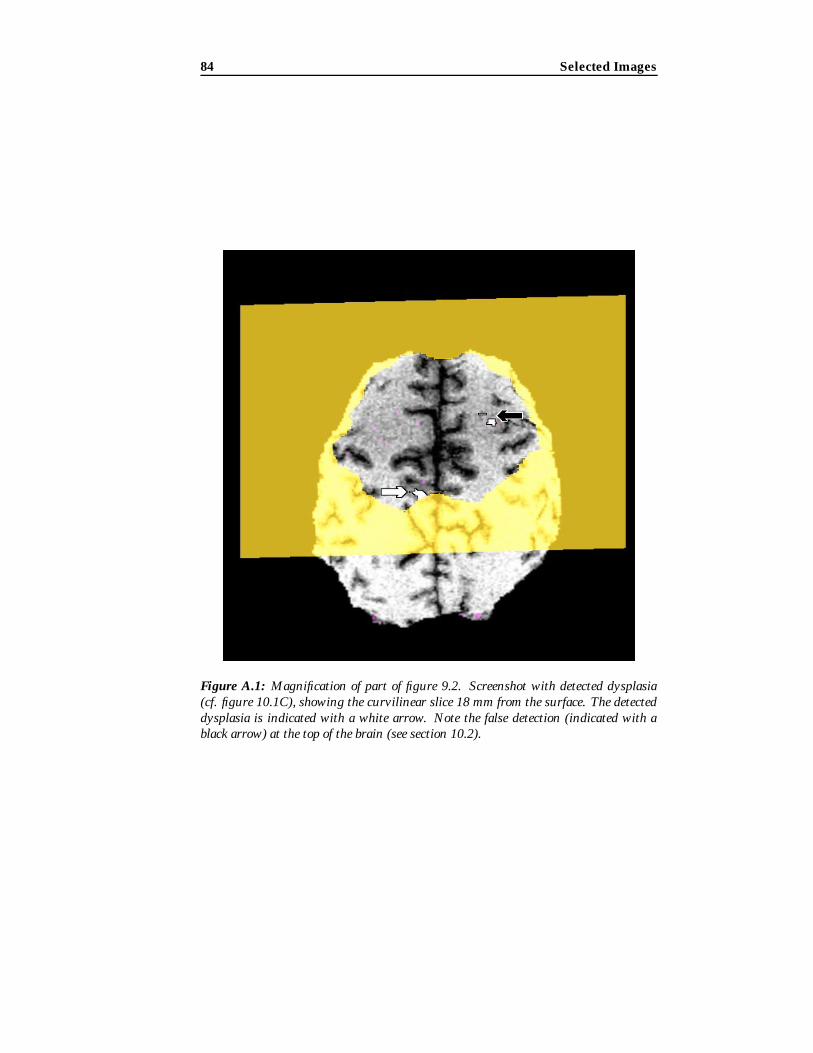
84 Selected Images
Figure A.1: Magnification of part of figure 9.2. Screenshot with detected dysplasia(cf. figure 10.1C), showing the curvilinear slice 18 mm from the surface. The detecteddysplasia is indicated with a white arrow. Note the false detection (indicated with ablack arrow) at the top of the brain (see section 10.2).
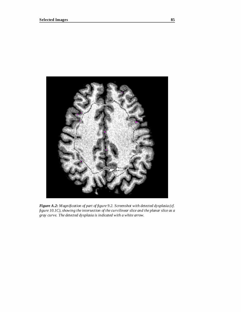
Selected Images 85
Figure A.2: Magnification of part of figure 9.2. Screenshot with detected dysplasia (cf.figure 10.1C), showing the intersection of the curvilinear slice and the planar slice as agray curve. The detected dysplasia is indicated with a white arrow.
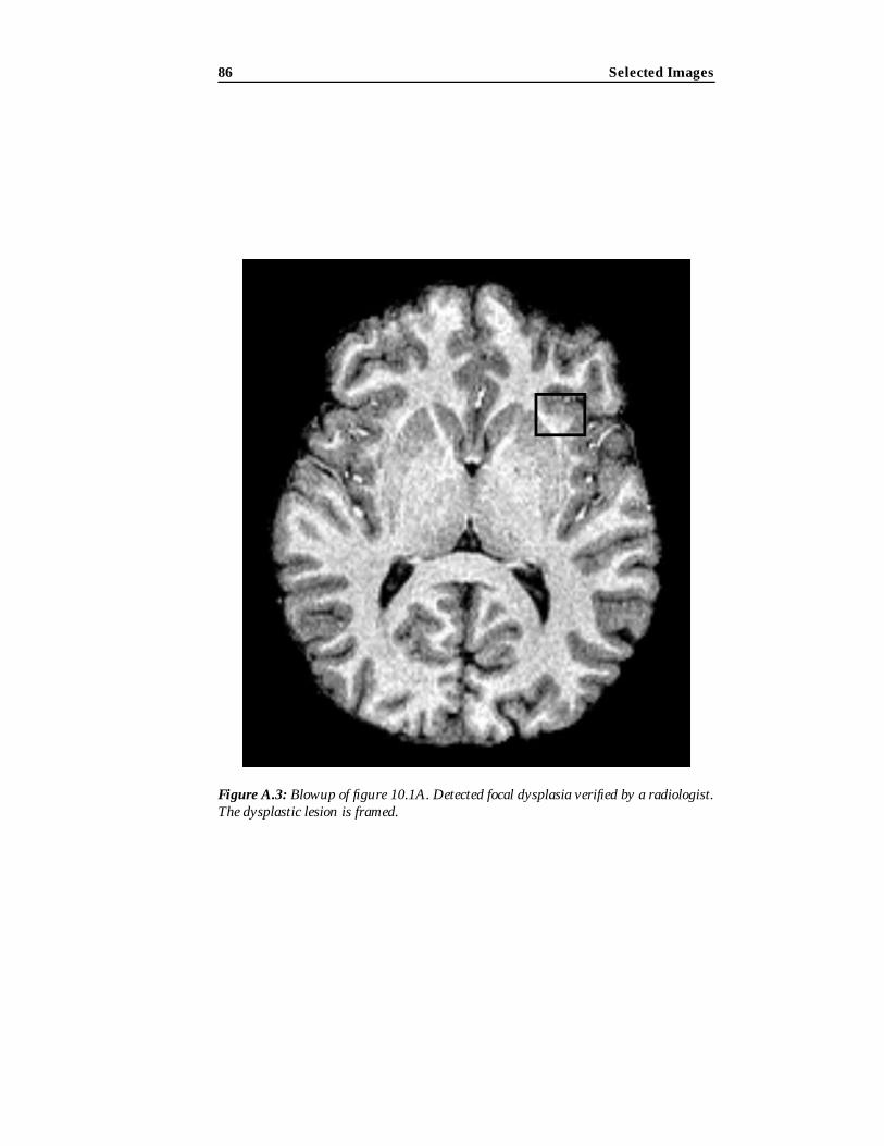
86 Selected Images
Figure A.3: Blowup of figure 10.1A. Detected focal dysplasia verified by a radiologist.The dysplastic lesion is framed.

Selected Images 87
Figure A.4: Magnification of figure 10.2A. Axial slice demonstrating the effects ofparameter variation in patient A. Lower correlation threshold set to 0:2. The dysplasiais indicated with white arrows, false detections with black arrows.

88 Selected Images
Figure A.5: Magnification of figure 10.2B. Axial slice demonstrating the effects ofparameter variation in patient A. Upper correlation threshold set to 0:9. The dysplasiais indicated with white arrows, false detections with black arrows.
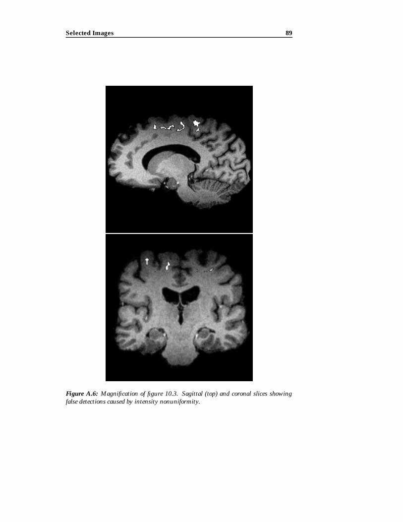
Selected Images 89
Figure A.6: Magnification of figure 10.3. Sagittal (top) and coronal slices showingfalse detections caused by intensity nonuniformity.


Appendix B
Resources on the Internet
The following addresses are valid at the time of writing (August 2001), but ow-ing to the dynamic nature of the internet, this may change in time.
� The FMRIB Software Library (Brain Extraction Tool):http://www.fmrib.ox.ac.uk/fsl
� A technical report on the Brain Extraction Tool (on-line version of [Smit00]):http://www.fmrib.ox.ac.uk/analysis/research/bet/bet/
� Abstract on detection of Focal Cortical Dysplasia by Voxel-Based Mor-phometry (on-line version of [Hupp01]):http://www.academicpress.com/www/journal/hbm2001/9991.html
� Article on template-based ray casting (on-line version of [Lee97]):http://cglab.snu.ac.kr/˜chlee/template.ps
� Philip Lacroute’s Ph.D thesis on shear-warp rendering (on-line version of[Lacr95]):http://www-graphics.stanford.edu/papers/lacroute thesis/
� Article on volumetric rendering using hardware accelerated pixel shad-ing (on-line version of [Enge01]):http://wwwvis.informatik.uni-stuttgart.de/˜engel/pre-integrated/


Bibliography
[Arno01] James B. Arnold, Jeih-San Liow, Kurt A. Schaper, Joshua J. Stern,John G. Sled, David W. Shattuck, Andrew J. Worth, Mark S. Cohen,Richard M. Leahy, John C. Mazziota, and David A. Rottenberg: Quali-tative and Quantitative Evaluation of Six Algorithms for Correcting In-tensity Nonuniformity Effects. NeuroImage 13, pp. 931-943, 2001.
[Ashb00] John Ashburner and Karl J. Friston: Voxel-Based Morphometry –The Methods. NeuroImage 11, pp. 805-821, 2000.
[Bast99] Alexandre C. Bastos, Roch M. Comeau, Frederick Andermann, DenisMelanson, Fernando Cendes, Francois Dubeau, Suzanne Fontaine, Do-natella Tampieri, and Andre Olivier: Diagnosis of Subtle Focal Dysplas-tic Lesions: Curvilinear Reformatting from Three-Dimensional MagneticResonance Imaging. Annals of Neurology, Vol 46, No 1, July 1999.
[Bran92] Michael Brant-Zawadzki, Gary D. Gillan, and Wolfgang R. Nitz:MPRAGE: A Three-Dimensional T1-Weighted Gradient Echo Sequence –Initial Experience in the Brain. Radiology 182(3), pp. 769-775, 1992.
[Came92] G. G. Cameron and P. E. Undrill: Rendering Volumetric Image Dataon a SIMD-Architecture Computer. Proceedings of the Third Eurograph-ics Workshop on Rendering, pp. 135-145, 1992.
[Cars00] Jens Michael Carstensen (Editor): Digital Image Processing. IMM,Technical University of Denmark, 2000.
[Corm97] Thomas H. Cormen, Charles E. Leiserson, Ronald L. Rivest: Intro-duction to Algorithms. ISBN: 0-262-53091-0. MIT Press, 1997.
[Edel96] Robert R. Edelman, Michael B. Zlatkin, John R. Hesselink, et al.: Clin-ical Magnetic Resonance Imaging, second edition. W.B. Saunders Com-pany, 1996.
[Enge01] Klaus Engel, Martin Kraus, and Thomas Ertl: High-Quality Pre-Integrated Volume Rendering Using Hardware-Accelerated Pixel Shad-ing. Eurographics / SIGGRAPH Workshop on Graphics Hardware ’01 (toappear), 2001.
[Fole97] James D. Foley, Andries van Dam, Stephen K. Feiner, John F. Hughes:Computer Graphics. Principle and Practice, second edition. ISBN 0-201-84840-6. Addison-Wesley, 1997.
[Fuch90] Henry Fuchs: Systems for Display of Three-Dimensional Medical Im-age Data, in: 3D Imaging in Medicine, ISBN: 3-540-52663-3. ISBN: 0-387-52663-3. Springer Verlag, 1990.
[Hans99] Vagn Lundsgaard Hansen: Fundamental Concepts in Modern Anal-ysis. ISBN 981-02-3894-0. World Scientific, 1999.
[Hupp01] Hans-Jurgen Huppertz, Jan Kassubek, Freimut D Jungling, Andreas
94 BIBLIOGRAPHY
Schulze-Bonhage: Detection of Focal Cortical Dysplasia by Voxel-BasedMorphometry. Abstract from the 7th Annual Meeting of the Organizationfor Human Brain Mapping 2001, NeuroImage, Academic Press, 2001.
[Klei85] F. Klein and O. Kubler: A Prebuffer Algorithm for Instant Displayof Volume Data. Proceedings of SPIE (Architectures and Algorithms forDigital Image Processing), Vol 596, pp. 54-58.
[Lacr95] Phillipe G. Lacroute: Fast Volume Rendering Using a Shear-WarpFactorization of the Viewing Transformation. PhD thesis, Stanford Uni-versity, September 1995.
[Lee97] Cheol-Hi Lee, Yun-Mo Koo, and Yeong Gil Shin: Template-Based Ren-dering of Run-Length Encoded Volumes. Proceedings of Pacific Graphics’97, pp. 139-147, 1997.
[Nibl86] Wayne Niblack: An Introduction to Digital Image Processing, ISBN0-13-480674-3. Prentice-Hall ltd, 1986.
[Nish94] Dwight G. Nishimura: Introduction to Magnetic Resonance Imaging.Course notes, Stanford University, 1994.
[Sait93] Toyofumi Saito and Jun-ichiro Toriwaki: Fast Algorithms for N-Dimensional Euclidean Distance Transformation. Proceedings of the 8thScandinavian Conference on Image Analysis, pp.747-754, 1993.
[Serr88] Jean Serra: Image Analysis and Mathematical Morphology vol 2: The-oretical Advances. ISBN 0-12-637241-1. Academic Press ltd, 1988.
[Smit00] Stephen M. Smith: BET: Brain Extraction Tool. FMRIB technical reportTR00SMS2, Oxford Centre for Functional Magnetic Resonance Imaging ofthe Brain, 2000. See also appendix B.
[Tayl71] D.C. Taylor, M.A. Falconer, C.J. Bruton, and J.A.N. Corsellis: FocalDysplasia of the Cerebral Cortex in Epilepsy. J. Neurol. Neurosurg. Psy-chiat., 34, 369-387, 1971.
[Zhan00] Yongyue Zhang, Stephen Smith, and Michael Brady: HiddenMarkov Random Field Model and Segmentation of Brain MR Images. FM-RIB Technical Report TR00YZ1, 2000.
[Wolf01] Stefan Wolff: Simulation af MR-skanning (in Danish). Project report,IMM, Technical University of Denmark, 2001.